Embed Size (px)
Citation preview
Semester Thesis
Stereoscopic Video Object Segmentation
based on Disparity Information for Robotics
Turgay Akdoğan
31. October 2012
Supervisor: Prof. Dr.-Ing. habil. Boris Lohmann
Advisor: Dipl.-Ing. Klaus J. Diepold
Institut: Lehrstuhl für Regelungstechnik
Technische Universität München

I assure the single handed composition of this Semester Thesis is only supported by
declared resources. I hereby agree to storage it permenantly in the Library of Chair
München, den March 8, 2013
Contents
Contents ii
List of Figures v
List of Tables vi
1. Introduction 1
1.1. Motivation . . . . . . . . . . . . . . . . . . . . . . . . . . . . . . . . . . . . 1
1.2. Summary of the Problem . . . . . . . . . . . . . . . . . . . . . . . . . . . . 3
2. Mathematical Background 6
2.1. An Introduction to Projective Geometry . . . . . . . . . . . . . . . . . . . 7
2.1.1. Coordinates . . . . . . . . . . . . . . . . . . . . . . . . . . . . . . . 8
2.2. Pinhole Camera Model . . . . . . . . . . . . . . . . . . . . . . . . . . . . . 9
2.3. Camera Calibration . . . . . . . . . . . . . . . . . . . . . . . . . . . . . . . 11
2.3.1. Intrinsic Parameters . . . . . . . . . . . . . . . . . . . . . . . . . . 15
2.3.2. Extrinsic Parameters . . . . . . . . . . . . . . . . . . . . . . . . . . 15
2.3.3. Camera Parameters Estimation . . . . . . . . . . . . . . . . . . . . 16
2.4. Epipolar Geometry . . . . . . . . . . . . . . . . . . . . . . . . . . . . . . . 20
2.5. Image Rectification . . . . . . . . . . . . . . . . . . . . . . . . . . . . . . . 22
2.6. Disparity Estimation . . . . . . . . . . . . . . . . . . . . . . . . . . . . . . 24
Contents ii
3. Disparity Based Segmentation 28
3.1. Basic Idea of Region Growing . . . . . . . . . . . . . . . . . . . . . . . . . 32
3.1.1. Single Regions . . . . . . . . . . . . . . . . . . . . . . . . . . . . . . 33
3.1.2. Multiple Region . . . . . . . . . . . . . . . . . . . . . . . . . . . . . 34
4. Proposed Solution 38
5. Conclusion 48
Bibliography 51
A. Appendix 52
A.1. Technical Data Sheet - Microsoft LifeCamStudio . . . . . . . . . . . . . . . 52
List of Figures
1.1. An example of 3D stereo image on left and corresponding disparity map on
right using Stereo images. (red colors indicate closer, blue colours represent pixels
that are farther away and dark blue colours indicate uncertainty pixels.) . . . . . . . 2
1.2. Ballbot without vision system. . . . . . . . . . . . . . . . . . . . . . . . . . 3
2.1. Stereo Camera System with pair of Microsoft LifeCam Studio webcams . . 6
2.2. Two parallel rails intersect in the image plane at the vanishing point [23]. . 7
2.3. A Pinhole Camera Model [21]. . . . . . . . . . . . . . . . . . . . . . . . . . 10
2.4. Single view geometry: the hole is called the camera center COP and the
image plane is placed between Object P and COP. Principal point where
is the center of image plane, is denoted by cc [18]. . . . . . . . . . . . . . . 10
2.5. Square and non-squared pixels . . . . . . . . . . . . . . . . . . . . . . . . . 13
2.6. The view from left camera a printed check-board pattern . . . . . . . . . . 16
2.7. The view from right camera a printed check-board pattern . . . . . . . . . 16
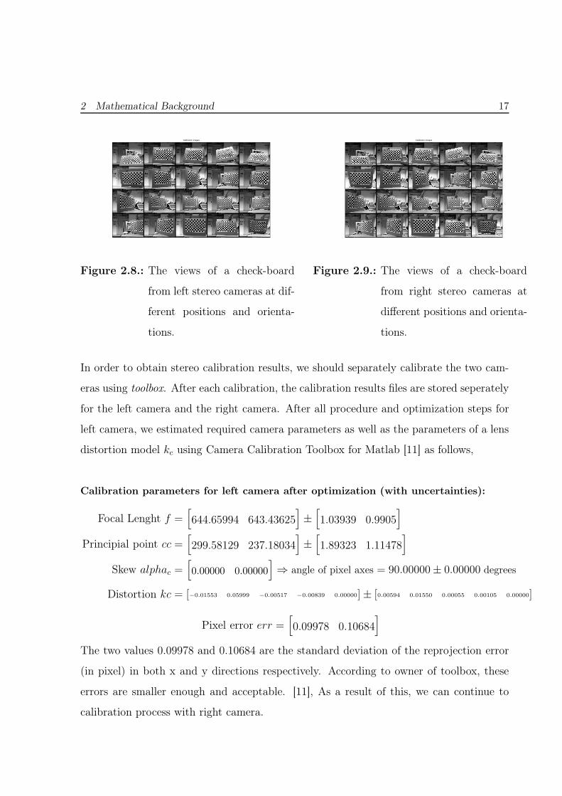
2.8. The views of a check-board from left stereo cameras at different positions
and orientations. . . . . . . . . . . . . . . . . . . . . . . . . . . . . . . . . 17
2.9. The views of a check-board from right stereo cameras at different positions
and orientations. . . . . . . . . . . . . . . . . . . . . . . . . . . . . . . . . 17
2.10. The extrinsic parameters of left camera are in a form of a 3D plot . . . . . 18
2.11. The extrinsic parameters of right camera are in a form of a 3D plot . . . . 19
2.12. The spatial configuration of the two cameras and the calibration planes are
in a form of a 3D plot . . . . . . . . . . . . . . . . . . . . . . . . . . . . . 20
List of Figures iv
2.13. Two cameras looking at a point X with their center of projection points OL
and OR. The projection of X onto left and right image planes are denoted
XL and XR. Points eL and eR are called epipoles [3]. . . . . . . . . . . . . 21
2.14. Epipolar Geometry after Rectification Process [17]. . . . . . . . . . . . . . 23
2.15. A potential matches between set of point correspondences of the rectified
images. . . . . . . . . . . . . . . . . . . . . . . . . . . . . . . . . . . . . . . 23
2.16. Rectified Stereo Images (Red - Left Image, Cyan - Right Image) . . . . . . 23
2.17. The disparity is estimated by finding best matching blocks along the epipo-
lar line in both images. . . . . . . . . . . . . . . . . . . . . . . . . . . . . . 24
2.18. Stereo camera model [19] . . . . . . . . . . . . . . . . . . . . . . . . . . . . 26
3.1. Framework of Hybrid Object Segmentation based on Intensity and Disparity 31
4.1. A rectified left image. . . . . . . . . . . . . . . . . . . . . . . . . . . . . . . 39
4.2. A rectified right image. . . . . . . . . . . . . . . . . . . . . . . . . . . . . . 39
4.3. Original Disparity Map . . . . . . . . . . . . . . . . . . . . . . . . . . . . . 39
4.4. Filtered Disparity Map . . . . . . . . . . . . . . . . . . . . . . . . . . . . . 40
4.5. Intensity Disparity Map . . . . . . . . . . . . . . . . . . . . . . . . . . . . 40
4.6. Binary Image from Intensity Disparity Map . . . . . . . . . . . . . . . . . 41
4.7. Area Openning in Binary Image . . . . . . . . . . . . . . . . . . . . . . . . 42
4.8. Filling image regions and holes, removing connected objects on borders if
they exist . . . . . . . . . . . . . . . . . . . . . . . . . . . . . . . . . . . . 43
4.9. 3D Coordinate of Extracted Objects in Real Scene . . . . . . . . . . . . . . 44
4.10. Toolbox in Real Scene . . . . . . . . . . . . . . . . . . . . . . . . . . . . . 44
4.11. Chair in Real Scene . . . . . . . . . . . . . . . . . . . . . . . . . . . . . . . 45
4.12. Chair and Toolbox in Real Scene . . . . . . . . . . . . . . . . . . . . . . . 45
4.13. Realtime Human Tracking . . . . . . . . . . . . . . . . . . . . . . . . . . . 46
4.14. Realtime Human Tracking . . . . . . . . . . . . . . . . . . . . . . . . . . . 46
4.15. Connected Objects (Static) . . . . . . . . . . . . . . . . . . . . . . . . . . 47

List of Figures v
4.16. Connected Objects (Dynamic) . . . . . . . . . . . . . . . . . . . . . . . . . 47

List of Tables
2.1. The four different geometries and the transformations allowed [10]. . . . . . 8
2.2. The XYW homogeneous coordinate space, a point P(X,Y,W) is projected
onto the W=1 plane [14]. . . . . . . . . . . . . . . . . . . . . . . . . . . . . 9
1. Introduction
1.1. Motivation
Computer vision is a field which one can use for acquiring, processing, analysing, and
understanding images such that in general, high-dimensional data from the real world
can be transformed into numerical information [2]. In this field using three dimensional
(3D) video which could be acquired by stereoscopic or multi-view camera systems, enables
to bring out a more realistic visual representation.
The object segmentation is one of the major tasks in computer vision. It is used for
locating any object in real world by using image processing. In other words it is a kind of
process that divides 2D image into meaningful segments. More precisely, the segmentation
is the process of assigning a label to every pixels in an image such that pixel with the
same label share certain visual characteristics such as disparity, intensity or texture. The
outcome of the image segmentation is a set of homogeneous regions which cover the entire
image. Every pixel in such homogeneous region shares the same characteristic [5].
The conventional object segmentation is renamed as mono segmentation in which
the source video is acquired from one camera. With the development the new capturing
devices, which enable to acquire video sequence in any condition, like stereoscopic or
multi-view camera systems etc., the object segmentation has become an important task in
multi-view video processing [26]. Using two cameras instead of one, give us the possibility
of locating the object. Stereoscopic video object segmentation is the main topic of this
Semester Thesis.
1 Introduction 2
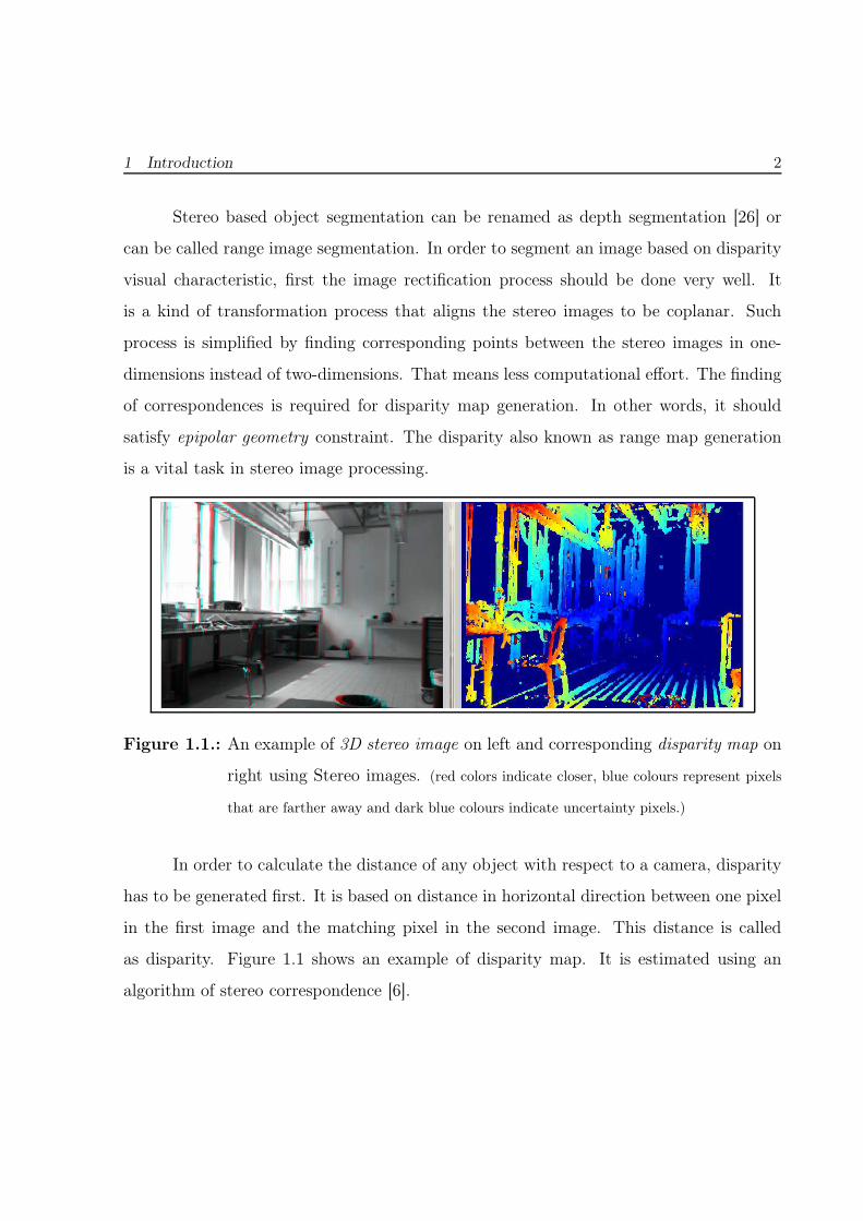
Stereo based object segmentation can be renamed as depth segmentation [26] or
can be called range image segmentation. In order to segment an image based on disparity
visual characteristic, first the image rectification process should be done very well. It
is a kind of transformation process that aligns the stereo images to be coplanar. Such
process is simplified by finding corresponding points between the stereo images in one-
dimensions instead of two-dimensions. That means less computational effort. The finding
of correspondences is required for disparity map generation. In other words, it should
satisfy epipolar geometry constraint. The disparity also known as range map generation
is a vital task in stereo image processing.
Figure 1.1.: An example of 3D stereo image on left and corresponding disparity map on
right using Stereo images. (red colors indicate closer, blue colours represent pixels
that are farther away and dark blue colours indicate uncertainty pixels.)
In order to calculate the distance of any object with respect to a camera, disparity
has to be generated first. It is based on distance in horizontal direction between one pixel
in the first image and the matching pixel in the second image. This distance is called
as disparity. Figure 1.1 shows an example of disparity map. It is estimated using an
algorithm of stereo correspondence [6].
1 Introduction 3
1.2. Summary of the Problem
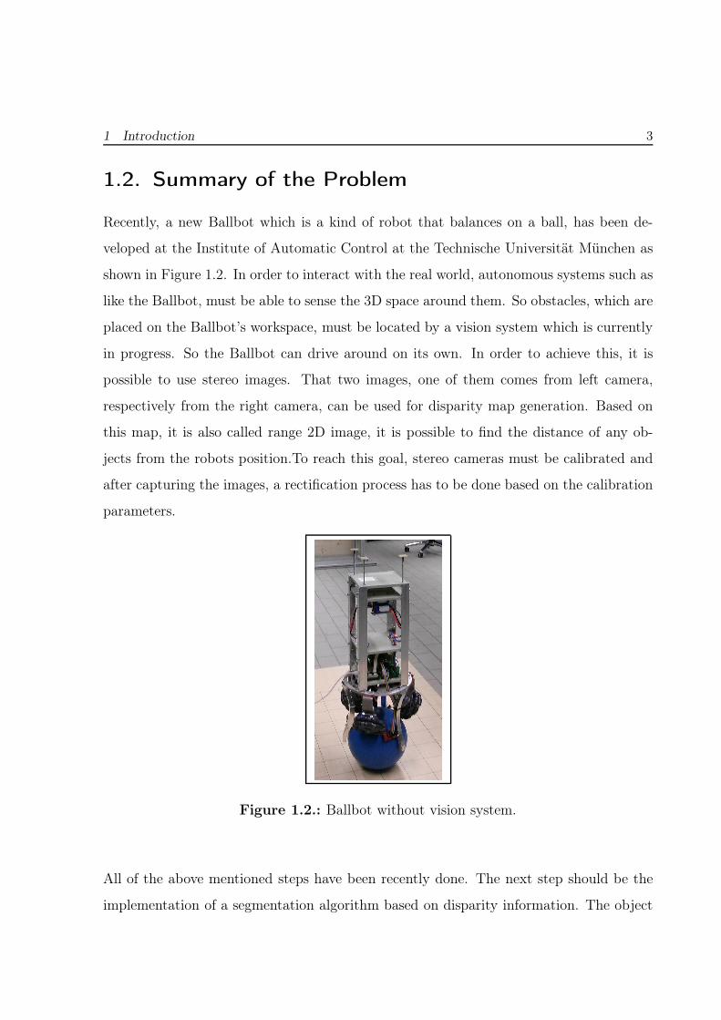
Recently, a new Ballbot which is a kind of robot that balances on a ball, has been de-
veloped at the Institute of Automatic Control at the Technische Universität München as
shown in Figure 1.2. In order to interact with the real world, autonomous systems such as
like the Ballbot, must be able to sense the 3D space around them. So obstacles, which are
placed on the Ballbot’s workspace, must be located by a vision system which is currently
in progress. So the Ballbot can drive around on its own. In order to achieve this, it is
possible to use stereo images. That two images, one of them comes from left camera,
respectively from the right camera, can be used for disparity map generation. Based on
this map, it is also called range 2D image, it is possible to find the distance of any ob-
jects from the robots position.To reach this goal, stereo cameras must be calibrated and
after capturing the images, a rectification process has to be done based on the calibration
parameters.
Figure 1.2.: Ballbot without vision system.
All of the above mentioned steps have been recently done. The next step should be the
implementation of a segmentation algorithm based on disparity information. The object
1 Introduction 4
segmentation is a kind of process that divides the images in meaningful region of pixels
belonging to the same object. One can get the location information of objects using this
technique.
The main goal of this Semester Thesis is describing an object segmentation technique
based on disparity map that has been already estimated previously in our project. Fur-
thermore, in order to achieve this, the essential Matlab code is implemented. In this
Thesis we will focus on this step.
1 Introduction 5
As mentioned in section 1.2 " Summary of the Problem " including the disparity esti-
mation all necessary steps for segmentation have been recently done. In the following
chapters we will be giving more briefly information such steps in computer vision. We
will be going further with segmentation based on disparity. For this purposes, several
general-purpose algorithms and techniques have been developed so far and the easiest
way to divide a 2D image into meaningful segments is called threshold method. This
method is based on an appropriate threshold value for each adjacent regions in an im-
age. With based on threshold method, we will be implementing a simple algorithm that
takes a sets of seeds as an input, for the segmentation process using Matlab development
environment.
The structure of this thesis is organized as follows. In Chapter 2, we give more brief infor-
mation for pre-processing step for segmentation. Chapter 3 describes the mathematical
background of the region-growing method used in segmentation. Chapter 4 introduces the
proposed solution for segmentation and experimental results are presented, Conclusion is
presented in Chapter 5.

2. Mathematical Background
In this chapter we lead the reader in a briefly overview through the pre-steps of object
segmentation using stereo images. In our case, we have used a pair of Microsoft LifeCam
Studio webcams (A.1.TDS) as shown in Figure 2.1, as stereo camera system. We start
with an introduction to projective geometry which has a vital importance in computer
vision.
Figure 2.1.: Stereo Camera System with pair of Microsoft LifeCam Studio webcams
Using its framework, it is possible to explain the pinhole camera model that one can obtain
the geometric relationship between a point in the real world and its corresponding point
in the captured 2D image. To do this, internal and external camera parameters which
give the location and setting of the camera, are introduced. To obtain such parameters
camera calibration is reviewed. Additionally, we proceed by reviewing of the geometric
framework. Finally we will be employing such obtained parameters throughout in this
semester thesis.
2 Mathematical Background 7
2.1. An Introduction to Projective Geometry
The Euclidean geometry describes our 3D world. In this geometry, the side of object
have lengths and the angles are determined by intersecting lines. It is said to be parallel
since the two lines lie in the same plane and never meet each other. Additionally, such
features don’t change when the translation and rotation are applied. It could be said that
with Euclidean geometry one can describe the world good enough but in case of image
processing, it becomes clear that Euclidean geometry is not sufficient in order to cope
with 2D image analysis. When we look at an 2D image, one can see squares that are
not squares, respectively circles that are not circles. Therefore we can said that acquired
images in 2D space, the lengths and angles are no longer preserved and might be intersect
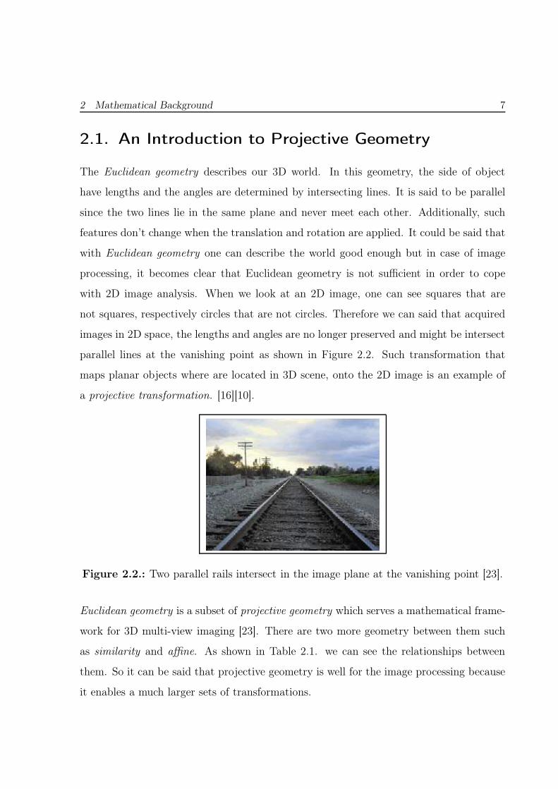
parallel lines at the vanishing point as shown in Figure 2.2. Such transformation that
maps planar objects where are located in 3D scene, onto the 2D image is an example of
a projective transformation. [16][10].
Figure 2.2.: Two parallel rails intersect in the image plane at the vanishing point [23].
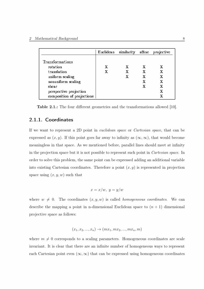
Euclidean geometry is a subset of projective geometry which serves a mathematical frame-
work for 3D multi-view imaging [23]. There are two more geometry between them such
as similarity and affine. As shown in Table 2.1. we can see the relationships between
them. So it can be said that projective geometry is well for the image processing because
it enables a much larger sets of transformations.
2 Mathematical Background 8
Table 2.1.: The four different geometries and the transformations allowed [10].
2.1.1. Coordinates
If we want to represent a 2D point in euclidean space or Cartesian space, that can be
expressed as (x, y). If this point goes far away to infinity as (∞,∞), that would become
meaningless in that space. As we mentioned before, parallel lines should meet at infinity
in the projection space but it is not possible to represent such point in Cartesian space. In
order to solve this problem, the same point can be expressed adding an additional variable
into existing Cartesian coordinates. Therefore a point (x, y) is represented in projection
space using (x, y, w) such that
x = x/w, y = y/w
where w 6= 0. The coordinates (x, y, w) is called homogeneous coordinates. We can
describe the mapping a point in n-dimensional Euclidean space to (n + 1) dimensional
projective space as follows:
(x1, x2, ..., xn) → (mx1, mx2, ..., mxn, m)
where m 6= 0 corresponds to a scaling parameters. Homogeneous coordinates are scale
invariant. It is clear that there are an infinite number of homogeneous ways to represent
each Cartesian point even (∞,∞) that can be expressed using homogeneous coordinates
2 Mathematical Background 9
as (x, y, 0). Additionally it would be much more useful way to go back and forward from
one coordinate of the point to another, simply by changing the last coordinate using
homogeneous coordinates.[16].
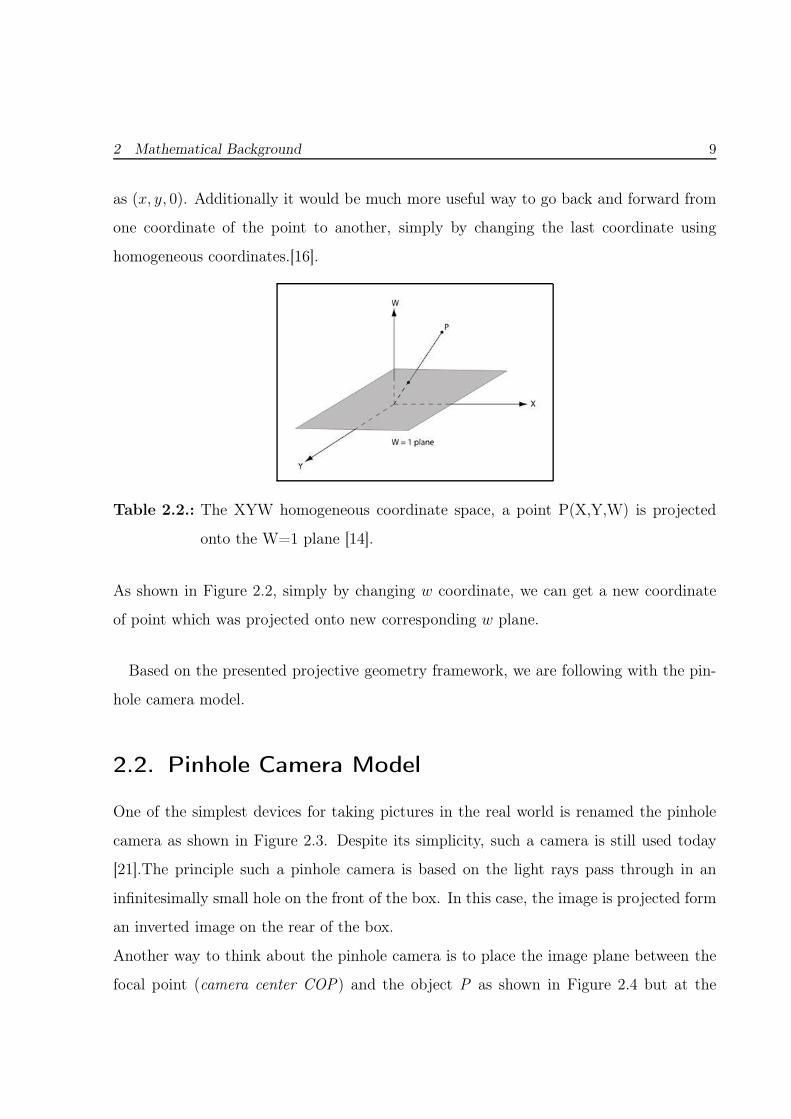
Table 2.2.: The XYW homogeneous coordinate space, a point P(X,Y,W) is projected
onto the W=1 plane [14].
As shown in Figure 2.2, simply by changing w coordinate, we can get a new coordinate
of point which was projected onto new corresponding w plane.
Based on the presented projective geometry framework, we are following with the pin-
hole camera model.
2.2. Pinhole Camera Model
One of the simplest devices for taking pictures in the real world is renamed the pinhole
camera as shown in Figure 2.3. Despite its simplicity, such a camera is still used today
[21].The principle such a pinhole camera is based on the light rays pass through in an
infinitesimally small hole on the front of the box. In this case, the image is projected form
an inverted image on the rear of the box.
Another way to think about the pinhole camera is to place the image plane between the
focal point (camera center COP) and the object P as shown in Figure 2.4 but at the
2 Mathematical Background 10
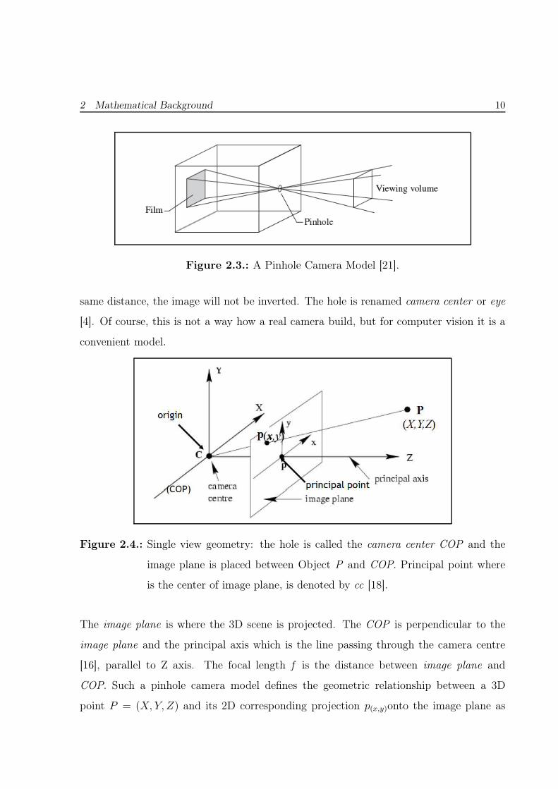
Figure 2.3.: A Pinhole Camera Model [21].
same distance, the image will not be inverted. The hole is renamed camera center or eye
[4]. Of course, this is not a way how a real camera build, but for computer vision it is a
convenient model.
Figure 2.4.: Single view geometry: the hole is called the camera center COP and the
image plane is placed between Object P and COP. Principal point where
is the center of image plane, is denoted by cc [18].
The image plane is where the 3D scene is projected. The COP is perpendicular to the
image plane and the principal axis which is the line passing through the camera centre
[16], parallel to Z axis. The focal length f is the distance between image plane and
COP. Such a pinhole camera model defines the geometric relationship between a 3D
point P = (X, Y, Z) and its 2D corresponding projection p(x,y)onto the image plane as
2 Mathematical Background 11
shown in Figure 2.4 . This geometric mapping from 3D to 2D is called a perspective
projection. Such projection lines pass through a single point onto image plane [6]. We
will briefly discuss more about the camera parameters in the following camera calibration
section.
2.3. Camera Calibration
Detailed information can be found in [1],[16],[20]. Camera calibration should be done
very carefully due to its importance in 3D computer vision in order to recover metric
information from 2D images. To define image coordinates p(x,y) with respect to the world
coordinates system, camera parameters are required. Such parameters determine a camera
characteristics.
We will obtain the camera projection matrix which is denoted CP . It is used for mapping
3D Point P to 2D point p(x,y) (see Figure 2.4).
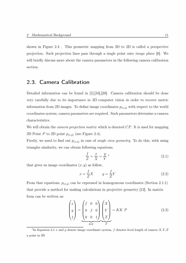
Firstly, we need to find out p(x,y) in case of single view geometry. To do this, with using
triangles similarity, we can obtain following equations.
f
Z=
x
X=
y
Y1 (2.1)
that gives us image coordinates (x, y) as follow,
x =f
ZX y =
f
ZY (2.2)
From that equations, p(x,y) can be expressed in homogeneous coordinates (Section 2.1.1)
that provide a method for making calculations in projective geometry [12]. In matrix
form can be written as:
x
y
1
=
f 0 0
0 f 0
0 0 1
︸ ︷︷ ︸
KK
X
Y
Z
︸ ︷︷ ︸
P
= KK P (2.3)
1In Equation 2.1 x and y denote image coordinate system, f denotes focal length of camera X,Y, Z
a point in 3D
2 Mathematical Background 12
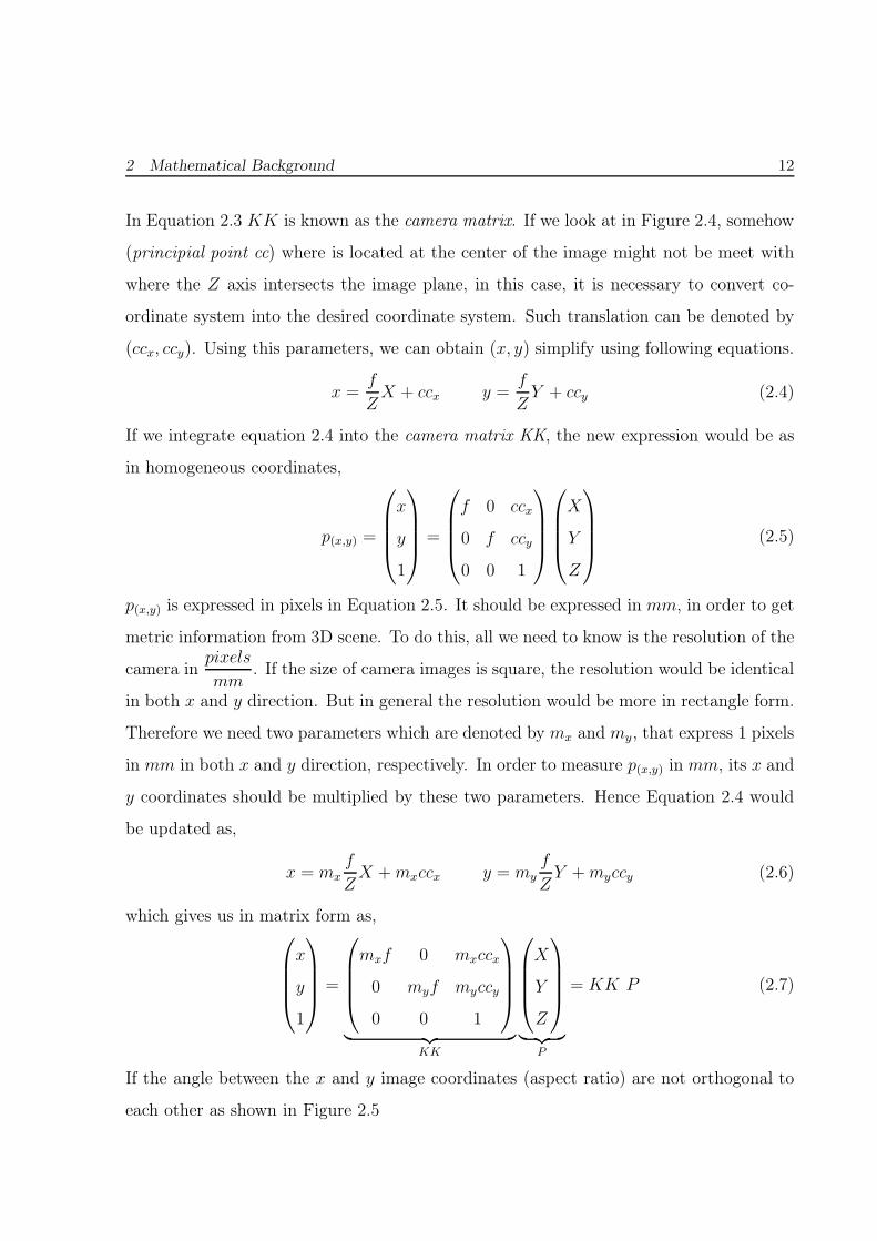
In Equation 2.3 KK is known as the camera matrix. If we look at in Figure 2.4, somehow
(principial point cc) where is located at the center of the image might not be meet with
where the Z axis intersects the image plane, in this case, it is necessary to convert co-
ordinate system into the desired coordinate system. Such translation can be denoted by
(ccx, ccy). Using this parameters, we can obtain (x, y) simplify using following equations.
x =f
ZX + ccx y =
f
ZY + ccy (2.4)
If we integrate equation 2.4 into the camera matrix KK, the new expression would be as
in homogeneous coordinates,
p(x,y) =
x
y
1
=
f 0 ccx
0 f ccy
0 0 1
X
Y
Z
(2.5)
p(x,y) is expressed in pixels in Equation 2.5. It should be expressed in mm, in order to get
metric information from 3D scene. To do this, all we need to know is the resolution of the
camera inpixels
mm. If the size of camera images is square, the resolution would be identical
in both x and y direction. But in general the resolution would be more in rectangle form.
Therefore we need two parameters which are denoted by mx and my, that express 1 pixels
in mm in both x and y direction, respectively. In order to measure p(x,y) in mm, its x and
y coordinates should be multiplied by these two parameters. Hence Equation 2.4 would
be updated as,
x = mx
f
ZX +mxccx y = my
f
ZY +myccy (2.6)
which gives us in matrix form as,
x
y
1
=
mxf 0 mxccx
0 myf myccy
0 0 1
︸ ︷︷ ︸
KK
X
Y
Z
︸ ︷︷ ︸
P
= KK P (2.7)
If the angle between the x and y image coordinates (aspect ratio) are not orthogonal to
each other as shown in Figure 2.5
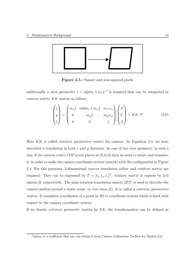
2 Mathematical Background 13
Figure 2.5.: Square and non-squared pixels
additionally a skew parameter s = alphac ∗ ccxf2 is required that can be integrated in
camera matrix KK matrix as follows,
x
y
1
=
mxf alphac ∗mxf mxccx
0 myf myccy
0 0 1
X
Y
Z
= KK P (2.8)
Here KK is called intrinsic parameters matrix for camera. In Equation 2.4, we have
described a translation in both x and y direction. In case of two view geometry, in such a
way, if the camera center COP is not places at (0, 0, 0) then we need to rotate and translate
it, in order to make the camera coordinate system coincide with the configuration in Figure
2.4. For this purposes, 3-dimensional camera translation vektor and rotation matrix are
required. They can be expressed by T = [tx, ty, tz]T , rotation matrix is express by 3x3
matrix R, respectively. The joint rotation-translation matrix [R|T ] is used to describe the
camera motion around a static scene, or vice versa [1]. It is called a extrinsic parameters
matrix. It translates coordinates of a point in 3D to coordinate system which is fixed with
respect to the camera coordinate system.
If we denote extrinsic parameter matrix by EE, the transformation can be defined as
2alphac is a coefficient that one can obtain it from Camera Calibration Toolbox for Matlab [11]
2 Mathematical Background 14
follows,
EE =
r11 r12 r13 tx
r21 r22 r23 ty
r31 r32 r33 tz
(2.9)
If we now want to express the camera projection matrix CP, in Equation 2.7 KK should
be multiplied by Equation 2.9 EE, that would be as follows,
CP =
mxf alphac ∗mxf mxccx
0 myf myccy
0 0 1
r11 r12 r13 tx
r21 r22 r23 ty
r31 r32 r33 tz
(2.10)
Hence, p(x,y) (see Figure 2.4) can be calculated by following equation, since translation
and rotation are required.
p(x,y) =
mxf alphac ∗mxf mxccx
0 myf myccy
0 0 1
r11 r12 r13 tx
r21 r22 r23 ty
r31 r32 r33 tz
X
Y
Z
1
(2.11)
As can be seen in CP matrix has 11 unknown intrinsic and extrinsic parameters such as 5
intrinsic, rotation (3-dimensional) and translation (3-dimensional). Such parameters can
be obtained using Camera Calibration Toolbox for Matlab [11]. In the following part,
we will give an overview of such camera parameters, afterwards we will be following with
estimation of camera parameters.
2 Mathematical Background 15
2.3.1. Intrinsic Parameters
Internal parameters characterize the optical, geometric, and digital characteristics of the
camera [9]
The list of Internal Parameters : [11]
• Focal Length f : Distance between the image plane and center of projection, focal
point or eye.
• Principal Point cc: The principal axis meets the image plane where the coordinate
of the pixels of a point. Such coordinates are stored in the 2x1 vector [ccxccy]
• Skew coefficient alphac: The skew coefficient defining the angle between the u
and v pixel axes is stored in the scalar alphac.
• Distortions kc: It models of the distortion of the lenses. Image distortion co-
efficients (radial and tangential distortions) are stored in the 5x1 vector kc. Once
distortion is applied corrected (final) pixel position [x; y] is obtained. The final pixel
coordinate and distorted pixel [xd; yd] coordinate are related to each other through
the linear equation as follows,
x
y
1
= KK
xd
yd
1
(2.12)
2.3.2. Extrinsic Parameters
Using the external camera parameters, we can find out the relationship between the
coordinate of a point P and camera Pc coordinates.
The list of External Parameters : [6]
2 Mathematical Background 16
• Rotation Matrix R: rotation in x,y,z direction between the orientation of the
camera coordinate system and the world coordinate system.
• Translation T: translation between the camera coordinate system and the origin
of the world coordinate system.
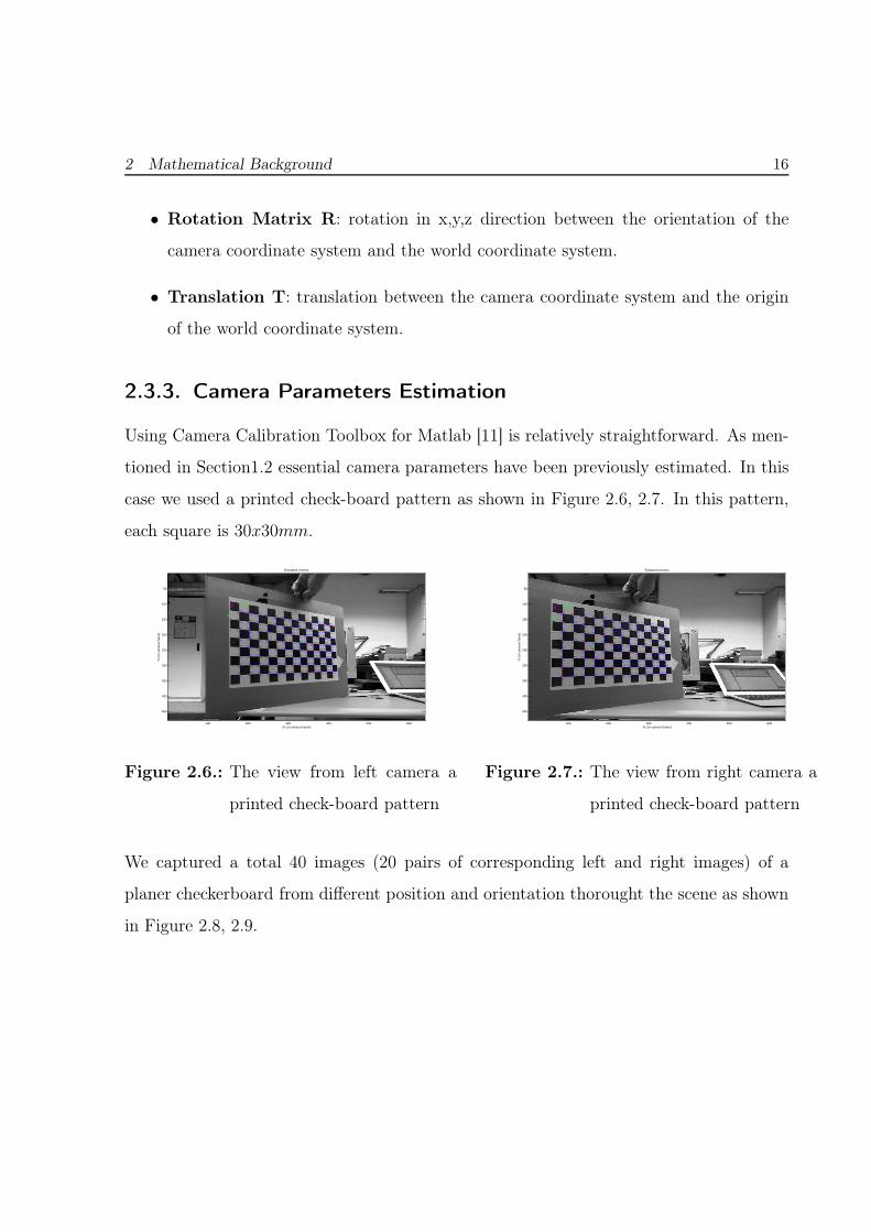
2.3.3. Camera Parameters Estimation
Using Camera Calibration Toolbox for Matlab [11] is relatively straightforward. As men-
tioned in Section1.2 essential camera parameters have been previously estimated. In this
case we used a printed check-board pattern as shown in Figure 2.6, 2.7. In this pattern,
each square is 30x30mm.
O
dX
dY
Xc (in camera frame)
Yc
(in c
amer
a fr
ame)
Extracted corners
100 200 300 400 500 600
50
100
150
200
250
300
350
400
450
Figure 2.6.: The view from left camera a
printed check-board pattern
O
dX
dY
Xc (in camera frame)
Yc
(in c
amer
a fr
ame)
Extracted corners
100 200 300 400 500 600
50
100
150
200
250
300
350
400
450
Figure 2.7.: The view from right camera a
printed check-board pattern
We captured a total 40 images (20 pairs of corresponding left and right images) of a
planer checkerboard from different position and orientation thorought the scene as shown
in Figure 2.8, 2.9.
2 Mathematical Background 17
Calibration images
Figure 2.8.: The views of a check-board
from left stereo cameras at dif-
ferent positions and orienta-
tions.
Calibration images
Figure 2.9.: The views of a check-board
from right stereo cameras at
different positions and orienta-
tions.
In order to obtain stereo calibration results, we should separately calibrate the two cam-
eras using toolbox. After each calibration, the calibration results files are stored seperately
for the left camera and the right camera. After all procedure and optimization steps for
left camera, we estimated required camera parameters as well as the parameters of a lens
distortion model kc using Camera Calibration Toolbox for Matlab [11] as follows,
Calibration parameters for left camera after optimization (with uncertainties):
Focal Lenght f =[
644.65994 643.43625]
±[
1.03939 0.9905]
Principial point cc =[
299.58129 237.18034]
±[
1.89323 1.11478]
Skew alphac =[
0.00000 0.00000
]
⇒ angle of pixel axes = 90.00000± 0.00000 degrees
Distortion kc = [−0.01553 0.05999 −0.00517 −0.00839 0.00000]± [0.00594 0.01550 0.00055 0.00105 0.00000]
Pixel error err =[
0.09978 0.10684]
The two values 0.09978 and 0.10684 are the standard deviation of the reprojection error
(in pixel) in both x and y directions respectively. According to owner of toolbox, these
errors are smaller enough and acceptable. [11], As a result of this, we can continue to
calibration process with right camera.
2 Mathematical Background 18
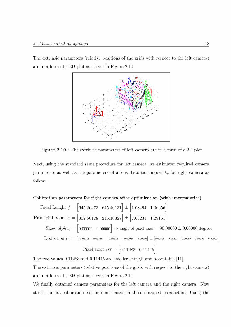
The extrinsic parameters (relative positions of the grids with respect to the left camera)
are in a form of a 3D plot as shown in Figure 2.10
Figure 2.10.: The extrinsic parameters of left camera are in a form of a 3D plot
Next, using the standard same procedure for left camera, we estimated required camera
parameters as well as the parameters of a lens distortion model kc for right camera as
follows,
Calibration parameters for right camera after optimization (with uncertainties):
Focal Lenght f =[
645.26473 645.40131]
±[
1.08494 1.06656]
Principial point cc =[
302.50128 246.10327]
±[
2.03231 1.29161]
Skew alphac =[
0.00000 0.00000
]
⇒ angle of pixel axes = 90.00000± 0.00000 degrees
Distortion kc = [−0.02111 0.09386 −0.00613 −0.00930 0.00000]± [0.00806 0.05203 0.00069 0.00106 0.00000]
Pixel error err =[
0.11283 0.11445]
The two values 0.11283 and 0.11445 are smaller enough and acceptable [11].
The extrinsic parameters (relative positions of the grids with respect to the right camera)
are in a form of a 3D plot as shown in Figure 2.11
We finally obtained camera parameters for the left camera and the right camera. Now
stereo camera calibration can be done based on these obtained parameters. Using the
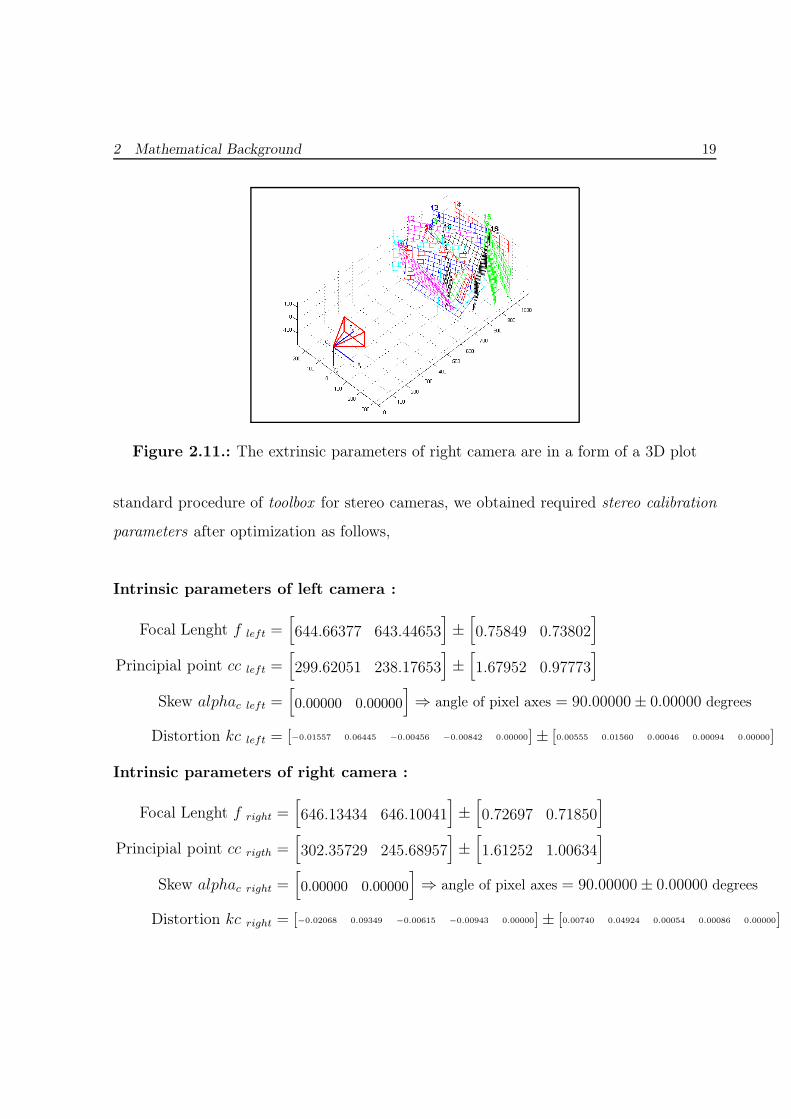
2 Mathematical Background 19
Figure 2.11.: The extrinsic parameters of right camera are in a form of a 3D plot
standard procedure of toolbox for stereo cameras, we obtained required stereo calibration
parameters after optimization as follows,
Intrinsic parameters of left camera :
Focal Lenght f left =[
644.66377 643.44653]
±[
0.75849 0.73802]
Principial point cc left =[
299.62051 238.17653]
±[
1.67952 0.97773]
Skew alphac left =[
0.00000 0.00000
]
⇒ angle of pixel axes = 90.00000± 0.00000 degrees
Distortion kc left = [−0.01557 0.06445 −0.00456 −0.00842 0.00000]± [0.00555 0.01560 0.00046 0.00094 0.00000]
Intrinsic parameters of right camera :
Focal Lenght f right =[
646.13434 646.10041]
±[
0.72697 0.71850]
Principial point cc rigth =[
302.35729 245.68957]
±[
1.61252 1.00634]
Skew alphac right =[
0.00000 0.00000
]
⇒ angle of pixel axes = 90.00000± 0.00000 degrees
Distortion kc right = [−0.02068 0.09349 −0.00615 −0.00943 0.00000]± [0.00740 0.04924 0.00054 0.00086 0.00000]
2 Mathematical Background 20
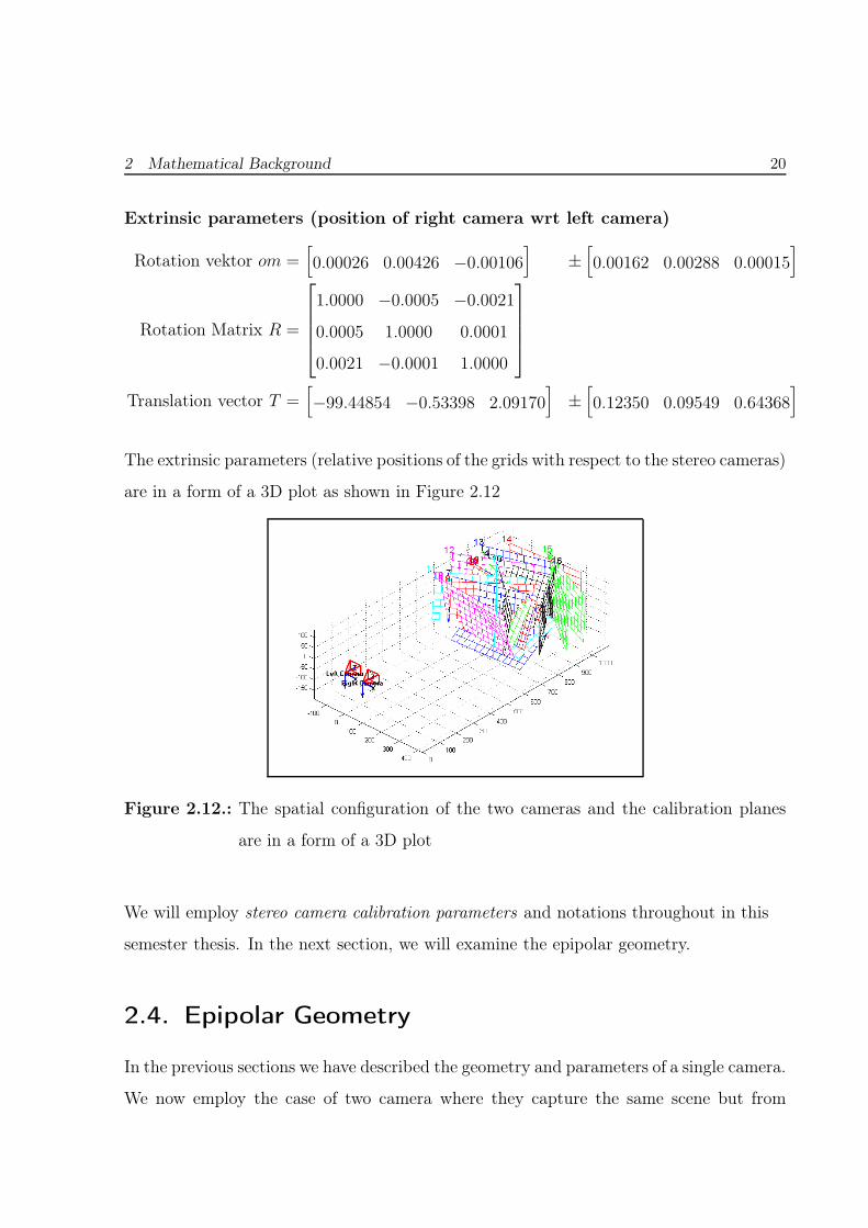
Extrinsic parameters (position of right camera wrt left camera)
Rotation vektor om =[
0.00026 0.00426 −0.00106]
±[
0.00162 0.00288 0.00015]
Rotation Matrix R =
1.0000 −0.0005 −0.0021
0.0005 1.0000 0.0001
0.0021 −0.0001 1.0000
Translation vector T =[
−99.44854 −0.53398 2.09170]
±[
0.12350 0.09549 0.64368]
The extrinsic parameters (relative positions of the grids with respect to the stereo cameras)
are in a form of a 3D plot as shown in Figure 2.12
Figure 2.12.: The spatial configuration of the two cameras and the calibration planes
are in a form of a 3D plot
We will employ stereo camera calibration parameters and notations throughout in this
semester thesis. In the next section, we will examine the epipolar geometry.
2.4. Epipolar Geometry
In the previous sections we have described the geometry and parameters of a single camera.
We now employ the case of two camera where they capture the same scene but from
2 Mathematical Background 21
distinct positions or viewpoints. If we want to estimate the 3D structure of the scene
from that two images, the estimation of the 3D points (X,X1, X2, X3) as shown in Figure
2.13 can be carried out since the epipolar geometry is used. To determine the distance to a
object in the scene, triangulation is used based on epipolar geometry. The definition of the
epipolar geometry can be expressed by geometrical relation between the two projection of
a 3D point which one can see this relation in Figure 2.13.
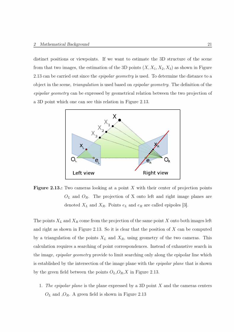
Figure 2.13.: Two cameras looking at a point X with their center of projection points
OL and OR. The projection of X onto left and right image planes are
denoted XL and XR. Points eL and eR are called epipoles [3].
The points XL and XR come from the projection of the same point X onto both images left
and right as shown in Figure 2.13. So it is clear that the position of X can be computed
by a triangulation of the points XL and XR, using geometry of the two cameras. This
calculation requires a searching of point correspondences. Instead of exhaustive search in
the image, epipolar geometry provide to limit searching only along the epipolar line which
is established by the intersection of the image plane with the epipolar plane that is shown
by the green field between the points OL,OR,X in Figure 2.13.
1. The epipolar plane is the plane expressed by a 3D point X and the cameras centers
OL and ,OR. A green field is shown in Figure 2.13
2 Mathematical Background 22
2. The epipolar line is the line established by the intersection of the image plane with
the epipolar plane. A red line is shown in Figure 2.13.
3. The baseline is the distance between the two cameras centers OL and OR .
4. The epipole is the point established by the intersection of the image plane with the
baseline eL and eR [23]
In order to simplify searching, images should be acquired in a proper way (perfect camera
alignment) such that all epipolar lines are parallel and horizontal. But in real case, it
is difficult to align and orient the two cameras such that epipolar lines are parallel and
horizontal [23]. Base on this reality, there is an alternative approach which is acquired
two views without any alignment and orientation. That approach transform both images
to be coplanar which provides parallel and horizontal epipolar lines. It is called image
rectification that will be explained in the following section.
2.5. Image Rectification
Image rectification is a kind of transformation process that aligns the stereo images to
be coplanar. In other words transforming epipolar lines of two images are horizontal and
parallel as shown in Figure 2.14.
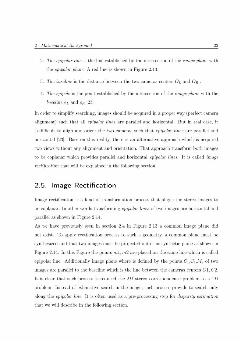
As we have previously seen in section 2.4 in Figure 2.13 a common image plane did
not exist. To apply rectification process to such a geometry, a common plane must be
synthesized and that two images must be projected onto this synthetic plane as shown in
Figure 2.14. In this Figure the points m1, m2 are placed on the same line which is called
epipolar line. Additionally image plane where is defined by the points C1,C2,M , of two
images are parallel to the baseline which is the line between the cameras centers C1, C2.
It is clear that such process is reduced the 2D stereo correspondence problem to a 1D
problem. Instead of exhaustive search in the image, such process provide to search only
along the epipolar line. It is often used as a pre-processing step for disparity estimation
that we will describe in the following section.
2 Mathematical Background 23
Figure 2.14.: Epipolar Geometry after Rectification Process [17].
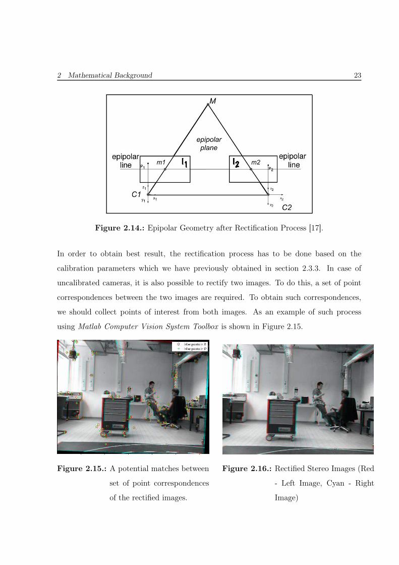
In order to obtain best result, the rectification process has to be done based on the
calibration parameters which we have previously obtained in section 2.3.3. In case of
uncalibrated cameras, it is also possible to rectify two images. To do this, a set of point
correspondences between the two images are required. To obtain such correspondences,
we should collect points of interest from both images. As an example of such process
using Matlab Computer Vision System Toolbox is shown in Figure 2.15.
Figure 2.15.: A potential matches between
set of point correspondences
of the rectified images.
Figure 2.16.: Rectified Stereo Images (Red
- Left Image, Cyan - Right
Image)
2 Mathematical Background 24
After cropping the overlapping area of the images in Figure 2.15, we obtain the rectified
images in Figure 2.16 . If we would look at the rectified images in Figure 2.16 using stereo
glasses, we would see 3D depth effect.
In the next section,disparity estimation is described based on the projective geometry
which we have seen in Section 2.1
2.6. Disparity Estimation
The disparity map is an image which stores the disparity values of all pixels, that has been
recently generated in Matlab. From this map, one can obtain location information of any
3D points in real world with respect to camera position since it has been converted to
depth map which is an image that represents the depth information of all pixels. Disparity
map can be estimated in matrix form that has the same size as the rectified images which
must be estimated one step before. In our case, the disparity computation has been done
based on simple Block Matching. Such a method is the most widely used for disparity
estimation in algorithm of stereo correspondence due to its simplicity and easiest way to
implement [15].
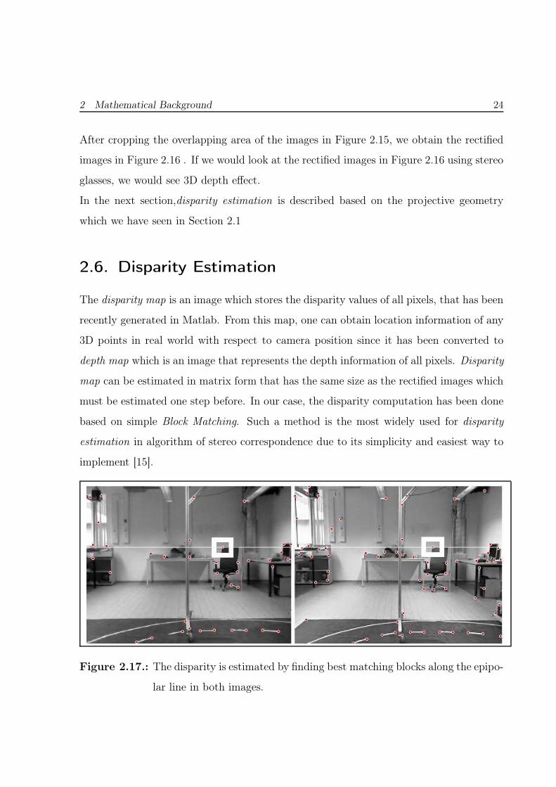
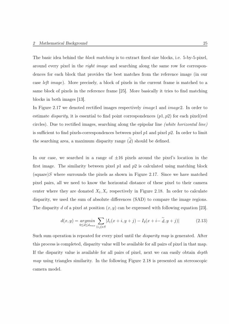
Figure 2.17.: The disparity is estimated by finding best matching blocks along the epipo-
lar line in both images.
2 Mathematical Background 25
The basic idea behind the block matching is to extract fixed size blocks, i.e. 5-by-5-pixel,
around every pixel in the right image and searching along the same row for correspon-
dences for each block that provides the best matches from the reference image (in our
case left image). More precisely, a block of pixels in the current frame is matched to a
same block of pixels in the reference frame [25]. More basically it tries to find matching
blocks in both images [13].
In Figure 2.17 we denoted rectified images respectively image1 and image2. In order to
estimate disparity, it is essential to find point correspondences (p1, p2) for each pixel(red
circles). Due to rectified images, searching along the epipolar line (white horizontal line)
is sufficient to find pixels-correspondences between pixel p1 and pixel p2. In order to limit
the searching area, a maximum disparity range (∼
d) should be defined.
In our case, we searched in a range of ±16 pixels around the pixel’s location in the
first image. The similarity between pixel p1 and p2 is calculated using matching block
(square)S where surrounds the pixels as shown in Figure 2.17. Since we have matched
pixel pairs, all we need to know the horizontal distance of these pixel to their camera
center where they are donated Xl, Xr respectively in Figure 2.18. In order to calculate
disparity, we used the sum of absolute differences (SAD) to compare the image regions.
The disparity d of a pixel at position (x, y) can be expressed with following equation [23].
d(x, y) = argmin0≤d≤dmax
∑
(i,j)ǫS
|I1(x+ i, y + j)− I2(x+ i−∼
d, y + j)| (2.13)
Such sum operation is repeated for every pixel until the disparity map is generated. After
this process is completed, disparity value will be available for all pairs of pixel in that map.
If the disparity value is available for all pairs of pixel, next we can easily obtain depth
map using triangles similarity. In the following Figure 2.18 is presented an stereoscopic
camera model.
2 Mathematical Background 26
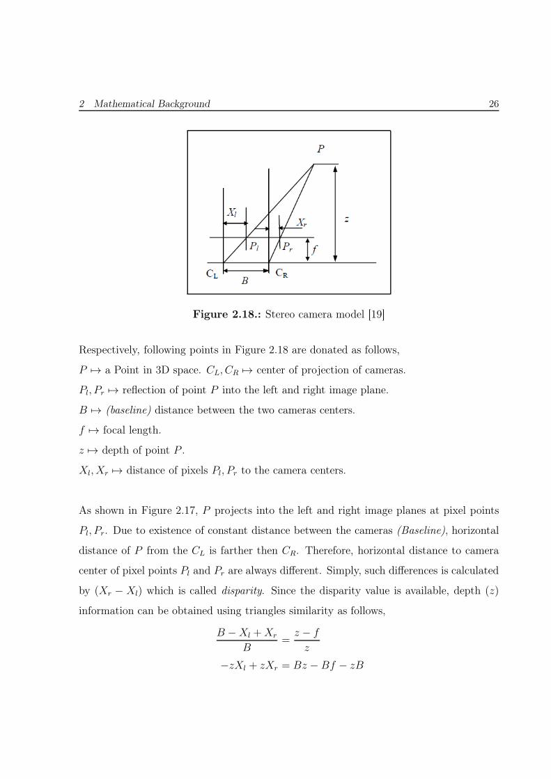
Figure 2.18.: Stereo camera model [19]
Respectively, following points in Figure 2.18 are donated as follows,
P 7→ a Point in 3D space. CL, CR 7→ center of projection of cameras.
Pl, Pr 7→ reflection of point P into the left and right image plane.
B 7→ (baseline) distance between the two cameras centers.
f 7→ focal length.
z 7→ depth of point P .
Xl, Xr 7→ distance of pixels Pl, Pr to the camera centers.
As shown in Figure 2.17, P projects into the left and right image planes at pixel points
Pl, Pr. Due to existence of constant distance between the cameras (Baseline), horizontal
distance of P from the CL is farther then CR. Therefore, horizontal distance to camera
center of pixel points Pl and Pr are always different. Simply, such differences is calculated
by (Xr − Xl) which is called disparity. Since the disparity value is available, depth (z)
information can be obtained using triangles similarity as follows,
B −Xl +Xr
B=
z − f
z
−zXl + zXr = Bz − Bf − zB
2 Mathematical Background 27
that gives us disparity equation as follows,
Xr −Xl = −Bf
z(2.14)
from this equation, one can say that disparity has the same meanings with depth in some
degree[19]. From this equations, depth (z) information can be expressed as follows,
z =Bf
Xl −Xr
(2.15)
Additionally, 3D location of P can be expressed as follows,
X =xr ∗ z
fY =
yr ∗ z
fZ =
Bf
Xl −Xr
(2.16)
Throughout Chapter 2, we have reviewed the required pre-processing steps for dispar-
ity based segmentation. In the following Chapter 3, region-based techniques for object
segmentation and its mathematical background is introduced.
3. Disparity Based Segmentation
In the previous Chapter 2 has been introduced required pre-steps for segmentation. Some
of the steps are calculated once, such as camera intrinsic and extrinsic parameters. In
other words, they are constant in our case. Because camera’s internal parameters are not
change in any condition, they are stored once, respectively if the stereo vision system is
mounted fixed on the top of the Ballbot as shown in Figure 2.1, camera external param-
eter is calculated just once too. Rest of the steps are done every time, such as image
rectification for every acquired stereo images and disparity estimation for every rectified
right image
.
After this short review of such steps, next we will be employing throughout this chapter
the process of segmentation. Before we start we should give more information about the
obtained disparity map in Matlab. Such a map is obtained as a matrix form in Matlab
workspace. Matrix size is equal to size of the right rectified images. As we have seen in
section 2.6, our reference image was right image.
If we run the code which has been implemented previously for such pre-steps for seg-
mentation, we can get an output 15 different range image every second, that corresponds
to 15 fps. In our case, such a speed is enough to cope with the real world. Using different
software development environment, development a different type of code or improving
hardware would increase the speed of disparity estimation.
3 Disparity Based Segmentation 29
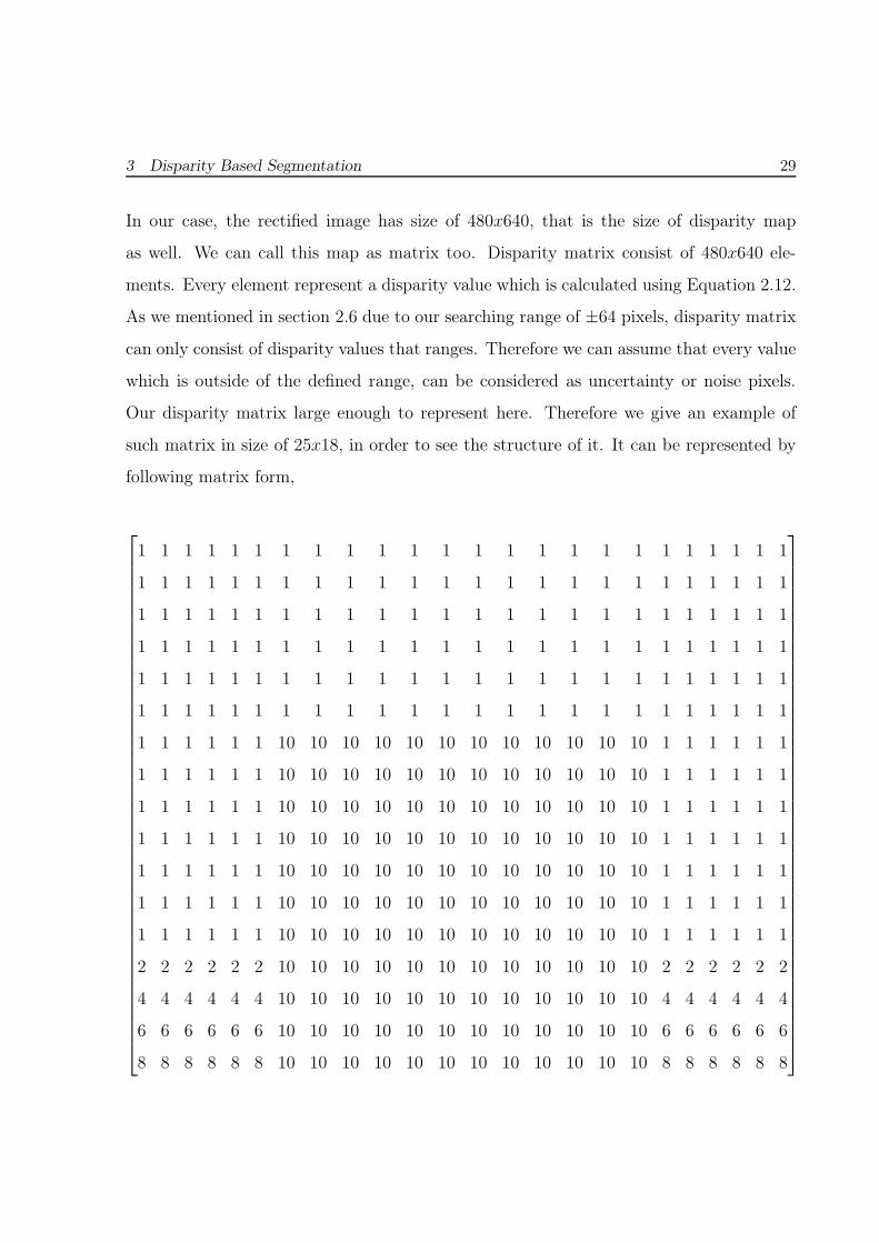
In our case, the rectified image has size of 480x640, that is the size of disparity map
as well. We can call this map as matrix too. Disparity matrix consist of 480x640 ele-
ments. Every element represent a disparity value which is calculated using Equation 2.12.
As we mentioned in section 2.6 due to our searching range of ±64 pixels, disparity matrix
can only consist of disparity values that ranges. Therefore we can assume that every value
which is outside of the defined range, can be considered as uncertainty or noise pixels.
Our disparity matrix large enough to represent here. Therefore we give an example of
such matrix in size of 25x18, in order to see the structure of it. It can be represented by
following matrix form,
1 1 1 1 1 1 1 1 1 1 1 1 1 1 1 1 1 1 1 1 1 1 1 1
1 1 1 1 1 1 1 1 1 1 1 1 1 1 1 1 1 1 1 1 1 1 1 1
1 1 1 1 1 1 1 1 1 1 1 1 1 1 1 1 1 1 1 1 1 1 1 1
1 1 1 1 1 1 1 1 1 1 1 1 1 1 1 1 1 1 1 1 1 1 1 1
1 1 1 1 1 1 1 1 1 1 1 1 1 1 1 1 1 1 1 1 1 1 1 1
1 1 1 1 1 1 1 1 1 1 1 1 1 1 1 1 1 1 1 1 1 1 1 1
1 1 1 1 1 1 10 10 10 10 10 10 10 10 10 10 10 10 1 1 1 1 1 1
1 1 1 1 1 1 10 10 10 10 10 10 10 10 10 10 10 10 1 1 1 1 1 1
1 1 1 1 1 1 10 10 10 10 10 10 10 10 10 10 10 10 1 1 1 1 1 1
1 1 1 1 1 1 10 10 10 10 10 10 10 10 10 10 10 10 1 1 1 1 1 1
1 1 1 1 1 1 10 10 10 10 10 10 10 10 10 10 10 10 1 1 1 1 1 1
1 1 1 1 1 1 10 10 10 10 10 10 10 10 10 10 10 10 1 1 1 1 1 1
1 1 1 1 1 1 10 10 10 10 10 10 10 10 10 10 10 10 1 1 1 1 1 1
2 2 2 2 2 2 10 10 10 10 10 10 10 10 10 10 10 10 2 2 2 2 2 2
4 4 4 4 4 4 10 10 10 10 10 10 10 10 10 10 10 10 4 4 4 4 4 4
6 6 6 6 6 6 10 10 10 10 10 10 10 10 10 10 10 10 6 6 6 6 6 6
8 8 8 8 8 8 10 10 10 10 10 10 10 10 10 10 10 10 8 8 8 8 8 8
3 Disparity Based Segmentation 30
In this simple example of disparity matrix (range 1 to 10 ) was introduced by hand and
randomly. 10 disparity value indicates closer, and 1 number represent that are farther
away from the camera position. If we look at it, we can easily see that some coherent
regions (pixel similarities) exist in that matrix such as 10, 1, etc. and it is clear that dis-
continuities of values correspond to regions boundaries. If we assume that, disparity value
10 belong to an object and value 1 for background, all we have to do to find coressponding
coherent regions using proper algorithm in Matlab. After segmentation process, we can
assign disparity values to each of these regions. As a result of this, we will be having
disparity value every object which belongs to real scene.
Object segmentation is almost impossible when only single image analysis is performed
[7]. Therefore, it is required to use different image information, such as disparity and
intensity information which show usually different characteristics. Disparity based seg-
mentation gives reliable results within regions but unreliable results on object boundaries
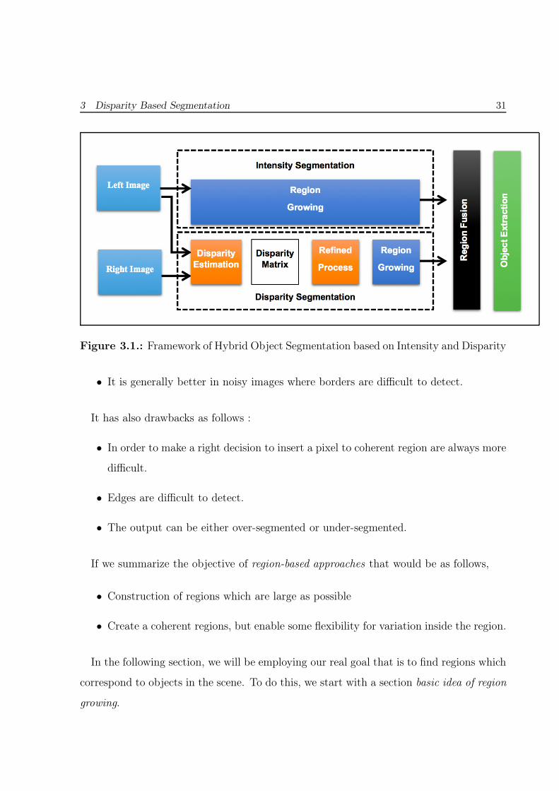
and intensity based segmentation gives just opposite results. Object is segmented by fusing
intensity and disparity segments information. Therfore, we propose to combine disparity
segmentation and intensity segmentation for object segmentation. It is called the hybrid
object segmentation. Framework can be seen in Figure 3.1. Proposed algorithm does
not dependent on disparity quality and not suffer the noise problem too. To do this, the
right rectified image and their corresponding disparity matrix are seperately segmented
by using region-growing technique. The goal of this techniques are construction of coher-
ent regions for both images. The criteria for homogeneity is disparity level for disparity
matrix and gray level properties for rectified right image.
Region-based techniques has some advantages as follows:
• Region cover more pixels, that means more information available in order to char-
acterize that region.
• It works from the inside out, instead of the outside in.
3 Disparity Based Segmentation 31
Figure 3.1.: Framework of Hybrid Object Segmentation based on Intensity and Disparity
• It is generally better in noisy images where borders are difficult to detect.
It has also drawbacks as follows :
• In order to make a right decision to insert a pixel to coherent region are always more
difficult.
• Edges are difficult to detect.
• The output can be either over-segmented or under-segmented.
If we summarize the objective of region-based approaches that would be as follows,
• Construction of regions which are large as possible
• Create a coherent regions, but enable some flexibility for variation inside the region.
In the following section, we will be employing our real goal that is to find regions which
correspond to objects in the scene. To do this, we start with a section basic idea of region
growing.
3 Disparity Based Segmentation 32
3.1. Basic Idea of Region Growing
Detailed information can be found in [8],[22]. Assume that we start with a single pixel
p1 that can be called a seed pixel or starting pixel. Our goal is to expand from that pixel
p1 to create a homogeneous (coherent) region. Coherent regions contain pixels that share
some similar property. If we define a similarity condition S(i, j) such that it provides
a result, if pixel i and j are similar or not. Assume that, pixel p2 is similar to pixel
p1. Since the similarity condition S(p1, p2) > T meets for some threshold T (similarity
variation tolerance), we can insert pixel p2 to pixel p1’s region. We similarly consider the
neighbours of p2 and add them as well, since the similarity condition meets for selected
threshold value. If we continue this recursively, we have an algorithm to create and fill
such a coherent region. After this short introduction we give a basic formulation of the
problem as follows:
I =
m⋃
i=1
Ri and Ri ∩Rj = ∅, i 6= j1 (3.1)
from this formulation, region-based segmentation can be expressed as follows :
H(Ri) = true for all i
H(Ri ∪Rj) = false, i 6= j, Ri adjagent to Rj
(3.2)
it is clear that, segmentation depend on as follows,
• properties used
• similarity measure between properties
• similarity variance tolerance (T )
Next, we will be discussing a few common approaches in case of single regions and
multiple regions
1 I denotes the entire image, R1, R2, ..., Rm are finite set of regions, H denotes Homogeneous
3 Disparity Based Segmentation 33
3.1.1. Single Regions
3.1.1.1. Similarity Measures
In order to compare pixel values, one can use similarity measure. If the difference of pixels
value (p1, p2) less than similarity measures, candidate pixel is added to p1’s region.
3.1.1.2. Comparing depend on Original Seed Pixel
In this approach comparing is done based on single seed pixel by using S(p1, p2). Adding
pixel p2 (compare pixel) to the growing region is done based on similarity measure. It
consist of always same single seed pixel p1.
3.1.1.3. Comparing depend on Neighbour in Region
A second approaches can be defined as follows : If p1 is similar to p2 and if p2 is similar
to p3, that means, p1 and p3 is placed in the same region.
3.1.1.4. Comparing based on Region Statistics
Pixel p2 (compared pixel) is compared to the entire region which consist of pixel p1 alone.
In this region pixel p1 dominates. During the region growing, aggregate statistics are
calculated. Any new pixel p3 that may be inserted to this region is compared not to pixel
p1 or its already neighbour p2, but to these aggregate statistics.
One way to collect such statistic can be done based on mean value of the region pixels,
but when every new pixel is inserted, this mean value is updated.
3.1.1.5. Multiple Seeds
Another approach is to produce a region not based on single seed pixel, but a small set of
pixels that describes better the region statistics. To do that,not only region mean is used,
but also variance as well. That enables to produce more identical regions under varying
noise conditions.
3 Disparity Based Segmentation 34
3.1.1.6. Cumulative Differences
If pixel p2 is a neighbour pixel p1 and candidate pixel p3 is a neighbour of pixel p2, instead
of using S(p1, p2) or S(p2, p3), we can use S(p1, p2) + S(p2, p3). This is equivalent to
detecting the minimum-cost path from pixel p1 to p3 and using this as the basis for the
addition or rejection o pixel p3.
3.1.2. Multiple Region
3.1.2.1. Selecting Seed Points
One way to select seed pixel is to do by clicking a mouse inside a desired object in image.
This process is started by manually selecting. In case of automatically segmenting we
do not use such a way. If we scatter seed points around the image, that would fill all
of the image with a regions, but if the current seed pixels are not sufficient, we can add
additional seed pixels by selecting new pixels but not already placed in segmented regions.
3.1.2.2. Scanning
Every pixel can be a seed in case of multiple-seed approach. If two adjacent pixels are
similar, merge them into a single region. If two adjacent regions are entirely similar
enough, merge them as well. This kind of similarity is based on comparing the statistics
of each region. Eventually, this method will converge when no further such mergings are
possible.
3.1.2.3. Split and Merge Algorithm
Region splitting is the opposite of region merging. A combination of these algorithms can
be explained that entire image is considered as one region. If the entire region is coherent,
there will be no further modification. If the region does not satisfy the condition of
homogeneity, image is sequentially divided into four quadrants and repeatedly is applied
these steps to each new region, since such adjacent regions (squares) of varying size might
3 Disparity Based Segmentation 35
have similar characteristics. Finally we define a criterion for merging these regions into
larger regions from the bottom up, since such regions is larger then single pixels.
3.1.2.4. Hybrid Edge - Region Approaches
This approach is based on combining strengths of two methods which are region and
boundary based segmentation. If we identified two adjacent regions that are candidates
for merging, we can examine the boundary between them . If the boundary is sufficient
strengths, we keep the region separate. If the boundary between them is weak, we merge
them.
3 Disparity Based Segmentation 36
After short review of common approaches in case of single and multiple region, next we
should choose proper approach in order to reach our goal that is implementing of essential
Matlab code for segmentation. As we mentioned previous Chapter 2 in Section 2.6, in
order to limit the searching area, a maximum disparity range (∼
d) should be defined. In
our case, we searched in a range of ±64 pixels. That implies maximum 65 (0 → 64)
different coherent regions can exist in disparity map. The growing of these each regions
can be done based on single seed pixel by using similarity measure. Therefore, due to
searching disparity range, these regions should be defined by 65 single seed pixels in a
image (disparity map) which means multiple region exist in a image. From that point, an
algorithm should be implement in case of multiple regions. We know the value of every
selected seed pixels for similarity measure but we don’t know where they should be placed
in image, in order to expand from that seed points to create a homogeneous region. If
we consider not only segmentation but also whole process of vision system, such process
should be executed by automatically. To do this we can scatter seed points around the
image. That would start to fill all of the image with a regions.
The aim of segmentation in our project is to detect an object in real world. In our
case, we would like to employ only objects which can be consider as an obstacle. There-
fore we can define a threshold value for region size too. That can be a threshold value
for number of compared pixels in region. If the number of pixels don’t meet for some
threshold, we can consider that region does not exist, so we can ignore it. Additionally, of
course accuracy of segmentation can depend on quality of disparity map. One solution is
to reduce the number of discontinuity and mismatching area in disparity matrix. Hence,
we should consider any pixel value outside of the defined range, as uncertainty or noise
pixels. Therefore before we start to execute algorithm to build a coherent region, we can
apply a filter to eliminate all irrelevant value depend on defined searching range from
disparity matrix.

3 Disparity Based Segmentation 37
In the following Chapter 4, the process of segmentation using Matlab software devel-
opment enviroment’s powerful functions are introduced.
4. Proposed Solution
In this Chapter, the process of segmentation based on disparity map using Matlab soft-
ware development environment is explained. We lead the reader in a briefly overview the
corresponding Matlab functions for segmentation process. Such functions are performed
to detect object area in 2D image using region-growing techniques that have been previ-
ously introduced in Chapter 3. The objects of interest are segmented and 3D coordinates
of segmented objects wrt right camera are obtained.
The process of segmentation is performed according to the following steps:
Before we start segmentation process, we can define the vision range, where could be
desired robot’s workspace. Such process reduces the expensive of computation. For in-
stance, to define that range 0 to 3 meter, we should remove corrensponding range values
from the disparity map [0 64]. Based on camera internal and external parameters, the
disparity is smaller then 20 can be considered out of that range. Therefore, new disparity
map includes only the value higher then 20.
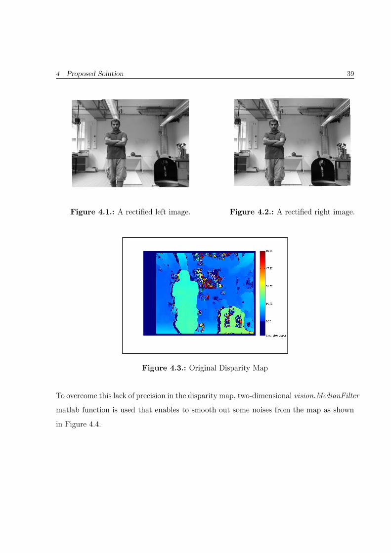
Disparity map might have noise which reduces the accuracy of map as shown in Figure
4.3.
4 Proposed Solution 39
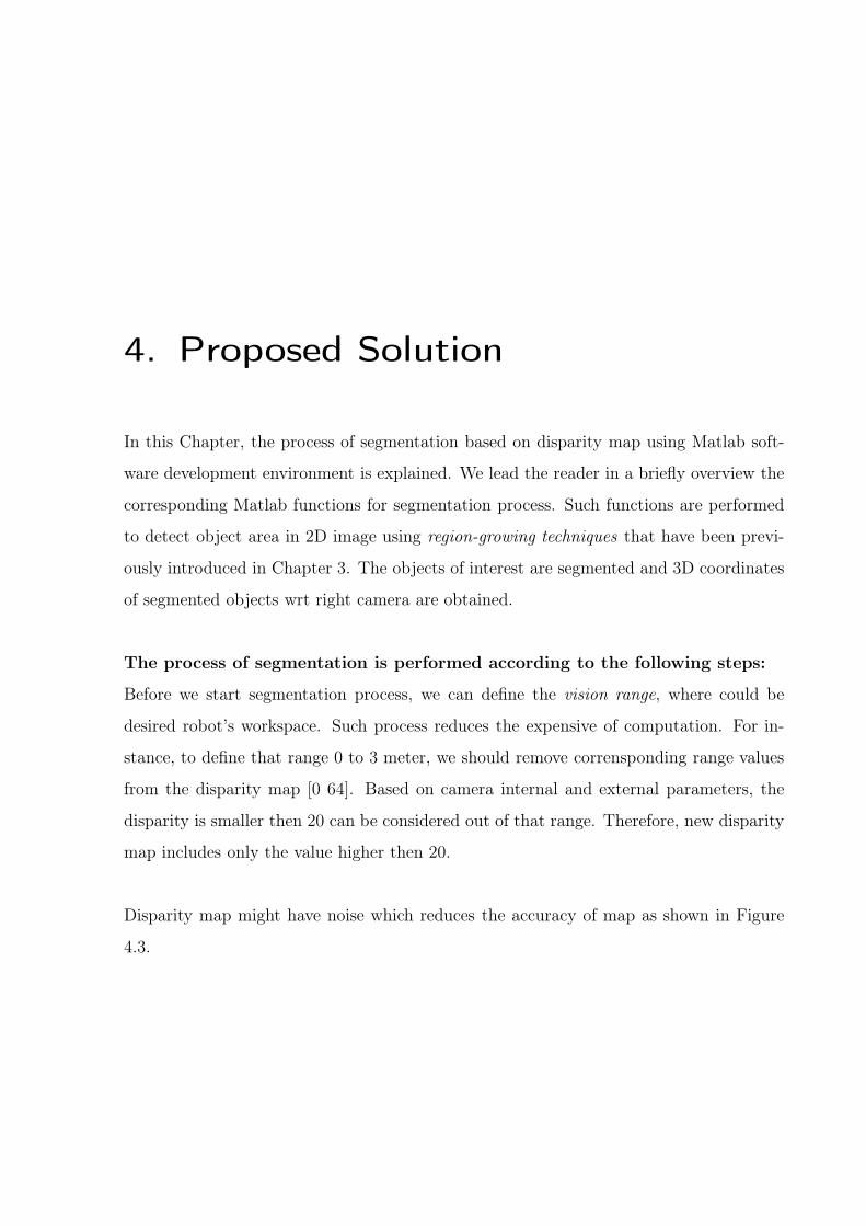
Figure 4.1.: A rectified left image. Figure 4.2.: A rectified right image.
Figure 4.3.: Original Disparity Map
To overcome this lack of precision in the disparity map, two-dimensional vision.MedianFilter
matlab function is used that enables to smooth out some noises from the map as shown
in Figure 4.4.
4 Proposed Solution 40
Figure 4.4.: Filtered Disparity Map
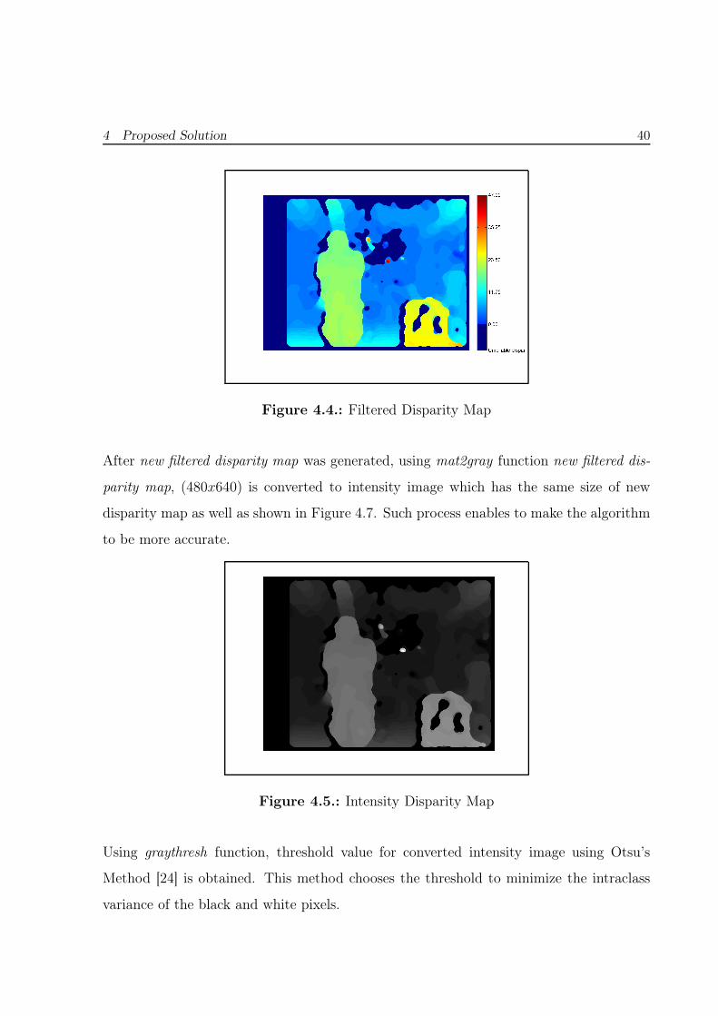
After new filtered disparity map was generated, using mat2gray function new filtered dis-
parity map, (480x640) is converted to intensity image which has the same size of new
disparity map as well as shown in Figure 4.7. Such process enables to make the algorithm
to be more accurate.
Figure 4.5.: Intensity Disparity Map
Using graythresh function, threshold value for converted intensity image using Otsu’s
Method [24] is obtained. This method chooses the threshold to minimize the intraclass
variance of the black and white pixels.
4 Proposed Solution 41
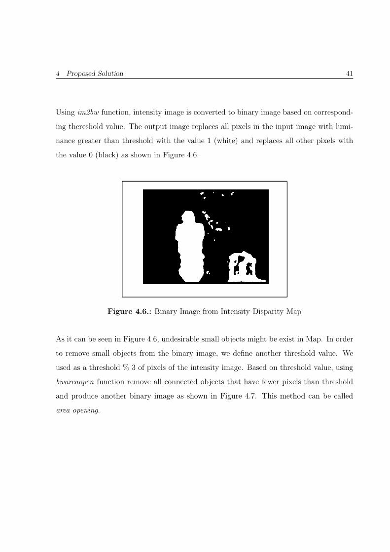
Using im2bw function, intensity image is converted to binary image based on correspond-
ing thereshold value. The output image replaces all pixels in the input image with lumi-
nance greater than threshold with the value 1 (white) and replaces all other pixels with
the value 0 (black) as shown in Figure 4.6.
Figure 4.6.: Binary Image from Intensity Disparity Map
As it can be seen in Figure 4.6, undesirable small objects might be exist in Map. In order
to remove small objects from the binary image, we define another threshold value. We
used as a threshold % 3 of pixels of the intensity image. Based on threshold value, using
bwareaopen function remove all connected objects that have fewer pixels than threshold
and produce another binary image as shown in Figure 4.7. This method can be called
area opening.
4 Proposed Solution 42
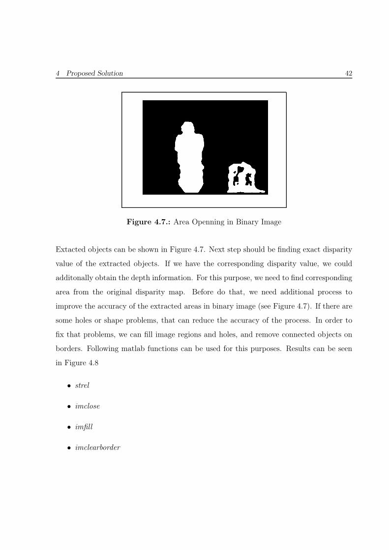
Figure 4.7.: Area Openning in Binary Image
Extacted objects can be shown in Figure 4.7. Next step should be finding exact disparity
value of the extracted objects. If we have the corresponding disparity value, we could
additonally obtain the depth information. For this purpose, we need to find corresponding
area from the original disparity map. Before do that, we need additional process to
improve the accuracy of the extracted areas in binary image (see Figure 4.7). If there are
some holes or shape problems, that can reduce the accuracy of the process. In order to
fix that problems, we can fill image regions and holes, and remove connected objects on
borders. Following matlab functions can be used for this purposes. Results can be seen
in Figure 4.8
• strel
• imclose
• imfill
• imclearborder

4 Proposed Solution 43
Figure 4.8.: Filling image regions and holes, removing connected objects on borders if
they exist
Finally, the segmentation process for desired objects has been completed. Using region-
props function, measure properties of extracted objects regions can be obtained such as
shape measurements and pixel value measurements. To find center coordinate of extracted
objects in Figure 4.7, we can use Centroid properties of regionprops function. Such op-
tion gives us 2-dimensional coordinate information of corresponding pixel in Binary Map.
Once we get 2-dimensional pixel coordinate information of extracted objects, we can ad-
ditionally obtain X and Y of 3D coordinates of corrensponding objects in real scene using
equation 2.11. To obtain exact disparity information of corresponding objects, we can
use PixelValues properties of regionprops function. Such option measures pixel values for
extracted object region in the Disparity Map. From this step, we will be having pixel
values for corresponding extracted object regions. But the problem is lacking of precision
in the disparity map. Some pixel values might have uncertanity values which reduces
the accuracy of exact disparity calculation, if we calculate an avarage of such values. To
overcome such problem we can find the most occurs pixel values in extracted regions. To
do this, we can use mode function which can tell us how many times it occurs in corre-
sponding extracted regions. Based on this result, we can assume that most occurs pixel
values should be the correct one. Based on exact disparity values of extracted region, we
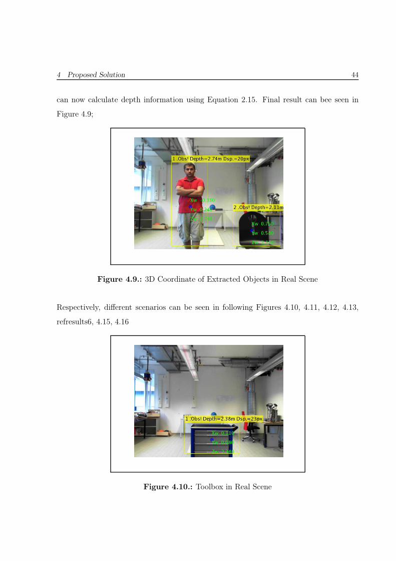
4 Proposed Solution 44
can now calculate depth information using Equation 2.15. Final result can bee seen in
Figure 4.9;
Figure 4.9.: 3D Coordinate of Extracted Objects in Real Scene
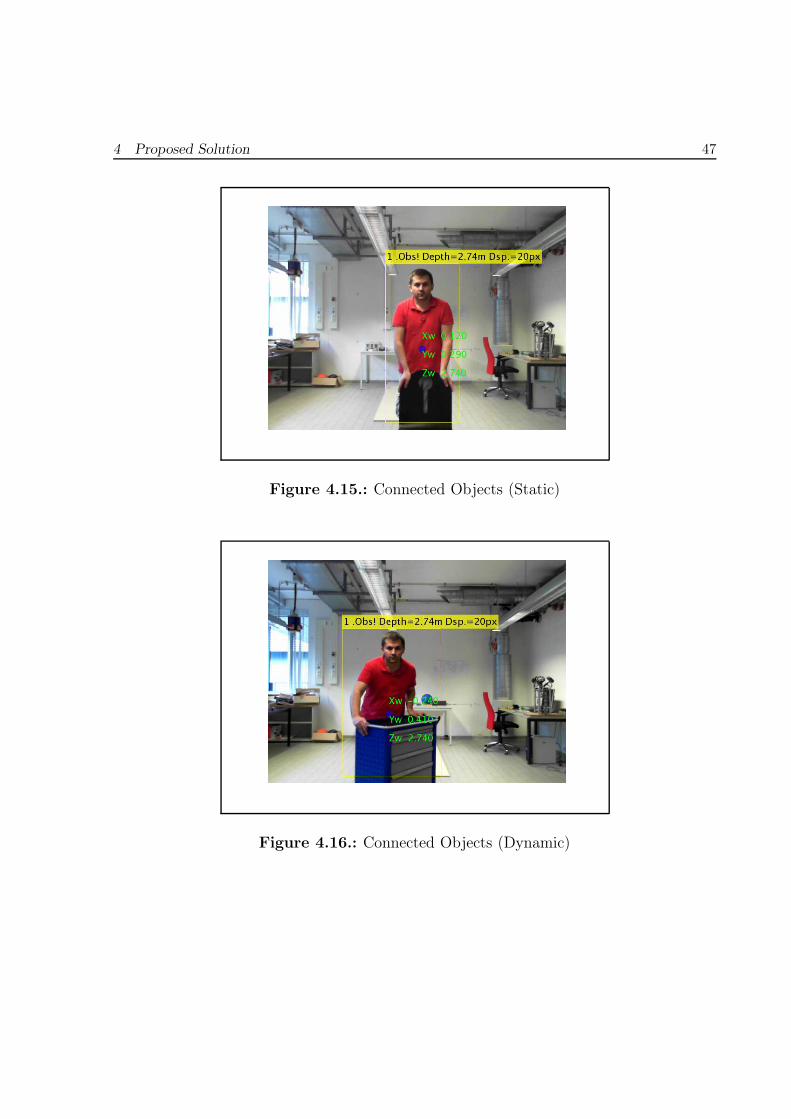
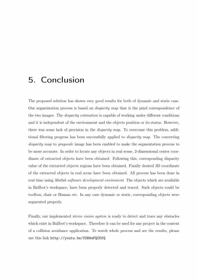
Respectively, different scenarios can be seen in following Figures 4.10, 4.11, 4.12, 4.13,
refresults6, 4.15, 4.16
Figure 4.10.: Toolbox in Real Scene
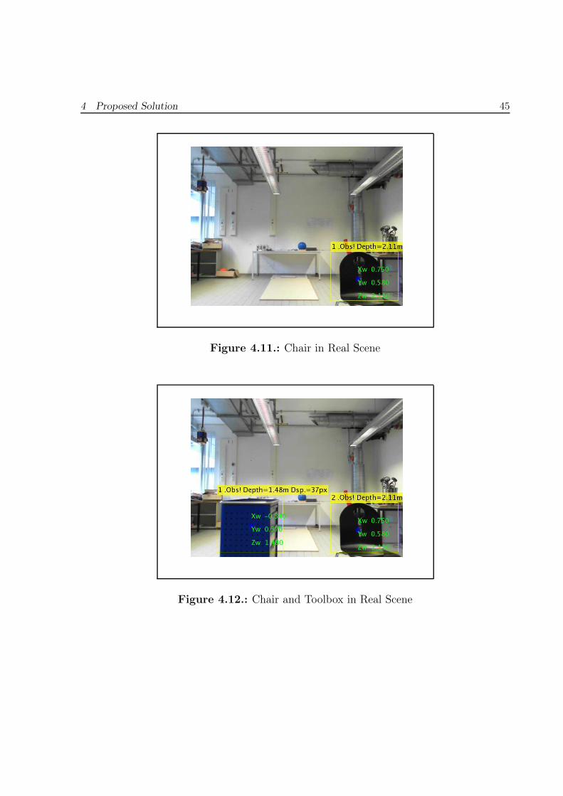
4 Proposed Solution 45
Figure 4.11.: Chair in Real Scene
Figure 4.12.: Chair and Toolbox in Real Scene
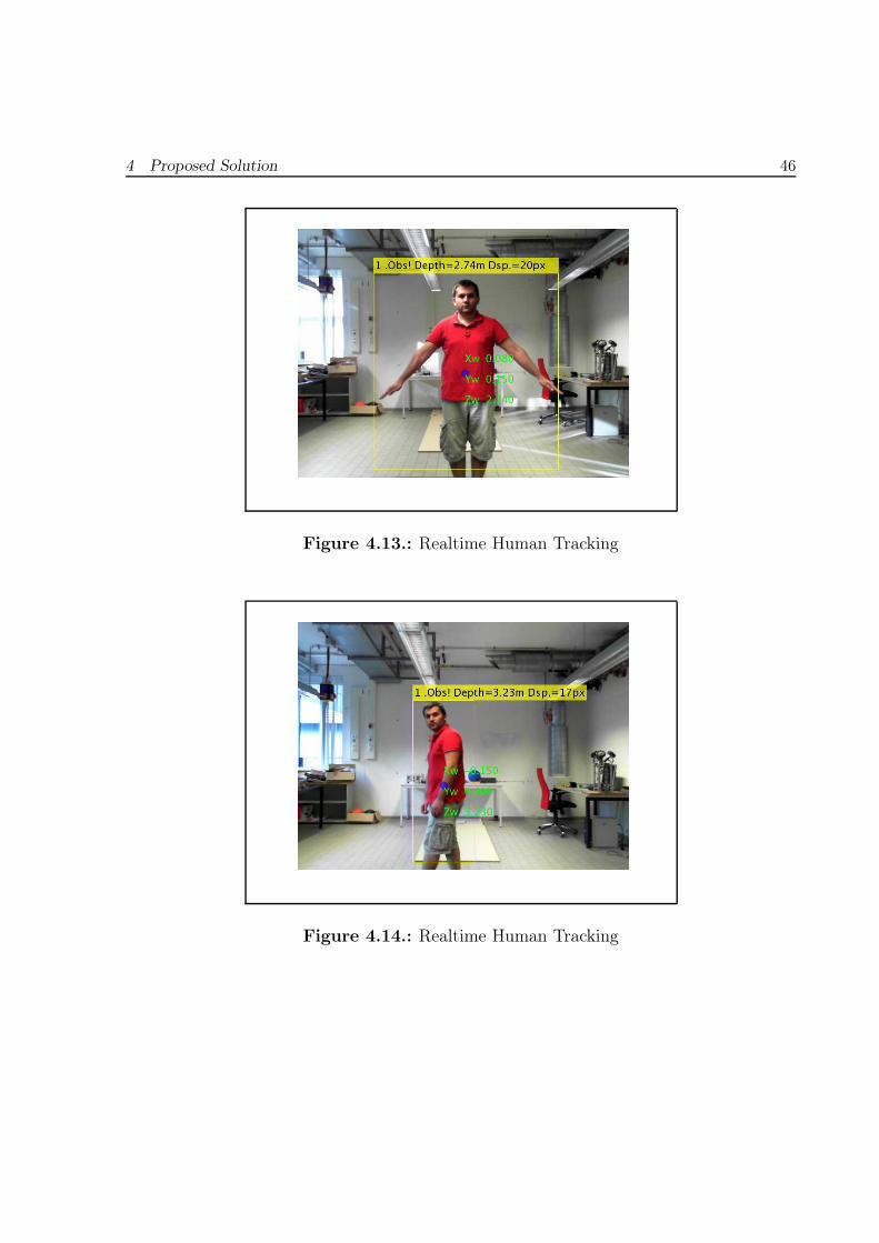
4 Proposed Solution 46
Figure 4.13.: Realtime Human Tracking
Figure 4.14.: Realtime Human Tracking
4 Proposed Solution 47
Figure 4.15.: Connected Objects (Static)
Figure 4.16.: Connected Objects (Dynamic)
5. Conclusion
The proposed solution has shown very good results for both of dynamic and static case.
Our segmentation process is based on disparity map that is the pixel correspondence of
the two images. The disparity estimation is capable of working under different conditions
and it is independent of the environment and the objects position or its status. However,
there was some lack of precision in the disparity map. To overcome this problem, addi-
tional filtering progress has been successfully applied to disparity map. The converting
disparity map to grayscale image has been enabled to make the segmentation process to
be more accurate. In order to locate any objects in real scene, 2-dimensional center coor-
dinate of extracted objects have been obtained. Following this, corresponding disparity
value of the extracted objects regions have been obtained. Finally desired 3D coordinate
of the extracted objects in real scene have been obtained. All process has been done in
real time using Matlab software development enviroment. The objects which are available
in Ballbot’s workspace, have been properly detected and traced. Such objects could be
toolbox, chair or Human etc. In any case dynamic or static, corresponding objects were
segmented properly.
Finally, our implemented stereo vision system is ready to detect and trace any obstacles
which exist in Ballbot’s workspace. Therefore it can be used for any project in the context
of a collision avoidance application. To watch whole process and see the results, please
use this link http://youtu.be/fDBWwFQCDfQ
Bibliography
[1] Camera Calibration and 3D Reconstruction - OpenCV 2.0 C Reference. http://
opencv.willowgarage.com/documentation/camera_calibration_and_3d_
reconstruction.html
[2] Computer vision - Wikipedia, the free encyclopedia. http://en.wikipedia.org/
wiki/Computer_vision
[3] Epipolar geometry - Wikipedia, the free encyclopedia. http://en.wikipedia.org/
wiki/Epipolar_geometry
[4] Pinhole camera - Wikipedia, the free encyclopedia. http://en.wikipedia.org/
wiki/Pinhole_camera
[5] Segmentation (image processing) - Wikipedia, the free encyclopedia. http://en.
wikipedia.org/wiki/Segmentation_(image_processing)
[6] Alegre, M. V.: Object segmentation based on the depth information. Institute of
Automation, University of Bremen, Diss., http://www.iat.uni-bremen.de/
sixcms/media.php/80/VictorMataFinalDoc_.pdf
[7] An, P. ; Lu, C. ; Zhang, Z.: Object segmentation using stereo images. In:
Communications, Circuits and Systems, 2004. ICCCAS 2004. 2004 International
Conference on Bd. 1, 2004, 534-538
[8] Ballard, D.H. ; Brown, C.M.: Computer vision. Prentice-Hall, 1982 http://
books.google.de/books?id=EfRRAAAAMAAJ. – ISBN 9780131653160
Bibliography 50
[9] Bebis, Dr. G.: Geometric Camera Parameters. http://www.cse.unr.edu/
~bebis/CS791E/Notes/CameraParameters.pdf. – Forschungsbericht
[10] Birchfield, Stan: An Introduction to Projective Geometry (for computer vision).
http://vision.stanford.edu/~birch/projective/
[11] Bouguet, Jean-Yves: Camera Calibration Toolbox for Matlab. http://www.
vision.caltech.edu/bouguetj/calib_doc/
[12] Davis, Tom: Homogeneous Coordinates and Computer Graphics. http://www.
geometer.org/mathcircles/cghomogen.pdf
[13] Florczyk, S.: Robot Vision. Wiley, 2006 http://books.google.de/books?
id=lhPI17ehuvkC. – ISBN 9783527604913
[14] FOLEY, VAN DAM A. FEINER S.K. Hughes J. J.D.: Computer Graphics -
Principles and Practice Second Edition in C. Addison-Wesley Publishing
Company., 1996
[15] Furht, B.: Encyclopedia of Multimedia. Springer, 2008 (Springer Reference).
http://books.google.de/books?id=Ipk5x-c_xNIC. – ISBN 9780387747248
[16] Hartley, R. I. ; Zisserman, A.: Multiple View Geometry in Computer Vision.
Second. Cambridge University Press, ISBN: 0521540518, 2004
[17] John P.H. Steele, Chris Debrunner Tyrone Vincent Stephen L. Chris Mnich M.
Chris Mnich: Development of closed-loop control of robotic welding processes.
Bd. 32. 4. An International Journal„ 2005. – 350 – 355 S.
[18] Li, Xin: Modeing the Pinhole Camera. http://www.math.ucf.edu/~xli/Pinhole
%20Camera2011.pdf. Version: 2012
[19] Lue Chaohui, ZHANG Q. YUAN Dun D. YUAN Dun: Stereoscopic video object
segmentation based on depth and edge information. 6625 (2007),
Bibliography 51
66250L–66250L-10. http://dx.doi.org/10.1117/12.790785. – DOI
10.1117/12.790785
[20] Majumder, Aditi: The Pinhole Camera. http://www.ics.uci.edu/~majumder/
vispercep/cameracalib.pdf
[21] Matt Pharr, Greg H. ; Todd Green, Heather S. (Hrsg.): Physically Based
Rendering. Second Edition. Elsevier, Inc, 2010. – 1200 S. – ISBN
978–0–12–375079–2
[22] Morse, Bryan S.: Segmentation ( Region Based ). Version: 2000. http://morse.
cs.byu.edu/~morse/
[23] Morvan, Yannick: Acquisition, Compression and Rendering of Depth and Texture
for Multi-View Video, Eindhoven University of Technology, Diss., June 9, 2009.
http://www.epixea.com/research/multi-view-coding-thesis.html
[24] Otsu, N: A Threshold Selection Method from Gray-Level Histograms. In: IEEE
Transactions on Systems, Man, and Cybernetics Vol. 9, No. 1 (1979), S. pp. 62–66
[25] Thyagarajan, K.S.: Still Image and Video Compression with MATLAB. Wiley,
2011 http://books.google.de/books?id=adv71MkRIWYC. – ISBN 9780470484166
[26] Zhang, Qian ; Liu, Suxing ; An, Ping ; Zhang, Zhaoyang: Object segmentation
based on disparity estimation. (2009), 1053–1056. http://dx.doi.org/10.1145/
1543834.1544006. – DOI 10.1145/1543834.1544006. ISBN 978–1–60558–326–6

A. Appendix
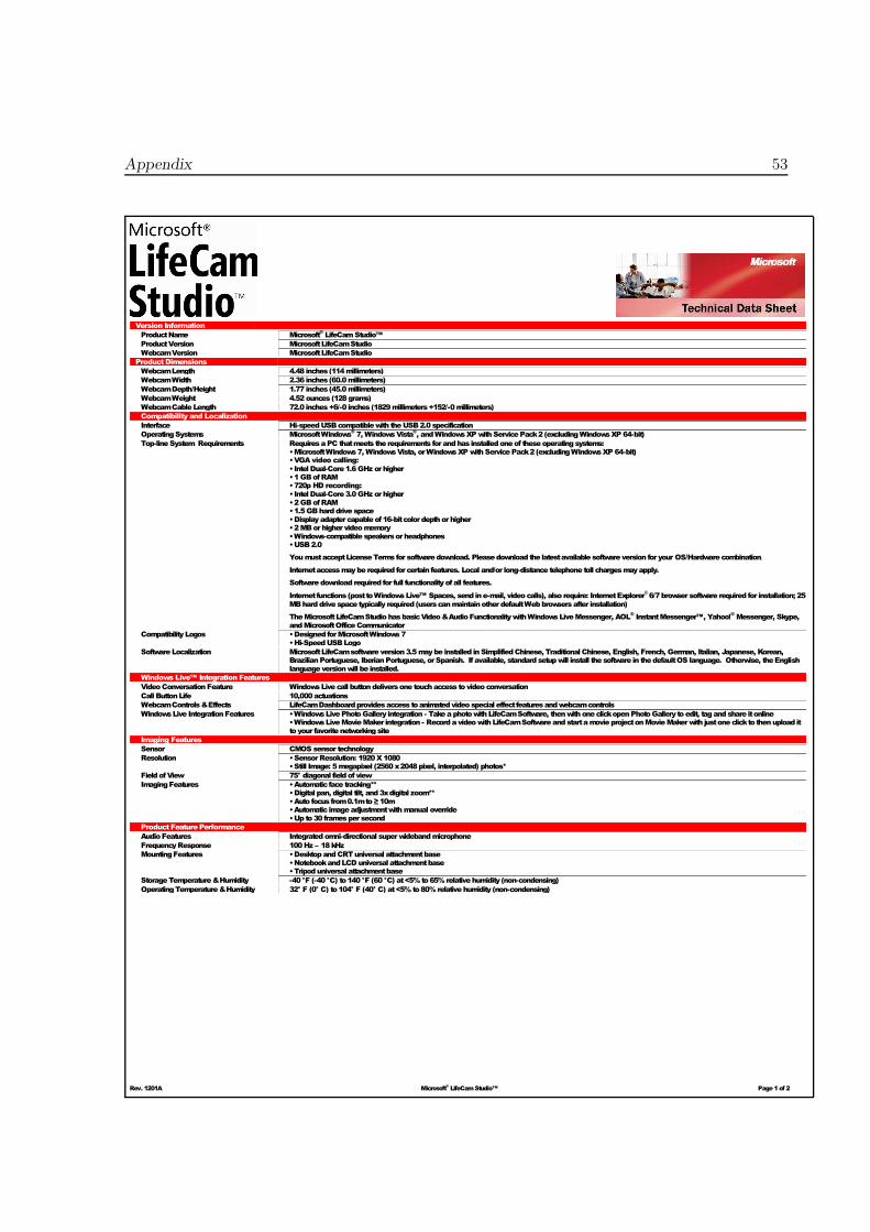
A.1. Technical Data Sheet - Microsoft LifeCamStudio
Appendix 53
Rev. 1201A Microsoft®LifeCamStudio™ Page1of 2
Version Information
ProductName Microsoft®LifeCamStudio™
ProductVersion MicrosoftLifeCamStudio
WebcamVersion MicrosoftLifeCamStudio
Product Dimensions
WebcamLength 4.48 inches(114millimeters)
WebcamWidth 2.36 inches(60.0millimeters)
WebcamDepth/Height 1.77 inches(45.0millimeters)
WebcamWeight 4.52ounces (128grams)
WebcamCableLength 72.0 inches+6/-0 inches (1829millimeters+152/-0millimeters)
Compatibility and Localization
Interface Hi-speedUSBcompatiblewith theUSB2.0specification
OperatingSystems MicrosoftWindows®7,WindowsVista
®, andWindowsXPwithServicePack2(excludingWindowsXP 64-bit)
Top-lineSystem Requirements RequiresaPC thatmeets the requirements forandhas installedoneof theseoperatingsystems:•MicrosoftWindows7,WindowsVista, orWindowsXPwithServicePack2(excludingWindowsXP 64-bit)• VGA video calling:
• Intel Dual-Core1.6GHz orhigher•1GBofRAM• 720p HD recording:• IntelDual-Core3.0GHz orhigher•2GBofRAM•1.5GBharddrivespace•Displayadaptercapableof16-bitcolordepthorhigher•2MBorhighervideomemory•Windows-compatiblespeakersorheadphones•USB2.0
YoumustacceptLicenseTerms for softwaredownload. Pleasedownload the latestavailablesoftwareversion for your OS/Hardwarecombination.
Internetaccessmaybe required forcertain features. Local and/or long-distance telephone toll chargesmayapply.
Softwaredownload required for full functionalityofall features.
Internetfunctions(posttoWindowsLive™ Spaces, send ine-mail, videocalls), also require: InternetExplorer®6/7browsersoftware required for installation; 25
MBharddrivespacetypically required (userscanmaintainotherdefaultWebbrowsersafter installation)
TheMicrosoftLifeCamStudiohasbasicVideo&AudioFunctionalitywithWindowsLiveMessenger, AOL®InstantMessenger™, Yahoo!
®Messenger, Skype,
andMicrosoftOfficeCommunicator
CompatibilityLogos •DesignedforMicrosoftWindows7•Hi-SpeedUSBLogo
SoftwareLocalization MicrosoftLifeCamsoftwareversion3.5maybe installed inSimplifiedChinese, TraditionalChinese, English, French, German, Italian, Japanese, Korean,BrazilianPortuguese, IberianPortuguese, orSpanish. If available, standardsetupwill install thesoftware in thedefaultOS language. Otherwise, theEnglishlanguageversionwill be installed.
Windows Live™ Integration Features
VideoConversationFeature WindowsLivecall buttondeliversone touchaccess tovideoconversation
Call ButtonLife 10,000actuations
WebcamControls&Effects LifeCamDashboardprovidesaccess toanimatedvideospecial effectfeaturesandwebcamcontrols
WindowsLive IntegrationFeatures •WindowsLivePhotoGallery integration - TakeaphotowithLifeCamSoftware, thenwithoneclickopenPhotoGallerytoedit, tagandshare itonline•WindowsLiveMovieMaker integration - RecordavideowithLifeCamSoftwareandstartamovieprojectonMovieMakerwith justoneclicktothenupload ittoyour favoritenetworkingsite
Imaging Features
Sensor CMOS sensor technology
Resolution •SensorResolution: 1920X1080•Still Image: 5megapixel (2560x2048pixel, interpolated) photos*
FieldofView 75° diagonal fieldof view
ImagingFeatures •Automaticface tracking**•Digital pan, digital tilt, and3xdigital zoom**•Auto focusfrom0.1mto≥10m•Automaticimageadjustmentwithmanual override•Up to30 framespersecond
Product Feature Performance
AudioFeatures Integratedomni-directional superwidebandmicrophone
FrequencyResponse 100Hz – 18kHz
MountingFeatures •DesktopandCRTuniversal attachmentbase•NotebookandLCD universalattachmentbase•Tripoduniversal attachmentbase
StorageTemperature&Humidity -40 °F (-40 °C) to140 °F (60 °C) at<5%to65%relativehumidity (non-condensing)
OperatingTemperature&Humidity 32° F (0° C) to104° F (40° C) at<5%to80%relativehumidity (non-condensing)