Embed Size (px)
Citation preview
Technische Universität MünchenFakultät für Elektrotechnik und Informationstechnik
Lehrstuhl für Informationstechnische Regelung
Safe Learning Control for Gaussian ProcessModels
Jonas Michael Umlauft
Vollständiger Abdruck der von der promotionsführenden Einrichtung Fakultät für Elek-trotechnik und Informationstechnik der Technischen Universität München zur Erlangungdes akademischen Grades eines
Doktor-Ingenieurs (Dr.-Ing.)
genehmigten Dissertation.
Vorsitzende/-r: Prof. Dr. sc. techn. Reinhard Heckel
Prüfende/-r der Dissertation:
1. Prof. Dr.-Ing. Sandra Hirche
2. Prof. Dr.-Ing. Matthias Müller
Die Dissertation wurde am 01.10.2019 bei der Technischen Universität München eingereichtund durch die promotionsführende Einrichtung Fakultät für Elektrotechnik und Informa-tionstechnik am 22.01.2020 angenommen.

PreambleThis thesis summarizes the conducted research at the Chair of Information-oriented Control(ITR) at the Technical University of Munich (TUM). I am very thankful for all the greatpeople that supported me during this time.First, I am truly grateful to my doctoral advisor, Prof. Sandra Hirche, who supported me
all the way from my undergraduate studies to my doctorate, always giving me the freedomto drive the research in my favorite direction. Her passion for scientific challenges and herconstant will to push our research in new directions always inspired me.Second, I would like to thank all the dedicated and gifted people, I had the pleasure to work
with at ITR. With his patience and his commitment to academic research, the supervisor ofmy bachelor’s thesis, Dominik Sieber, motivated me for this doctorate. My colleagues in thecon-humo project, José Ramón Medina, Satoshi Endo, Hendrik Börner, Melanie Kimmel andThomas Beckers, not just helped me to find the topic of this dissertation, but also inspiredme in many productive and fruitful discussions. A big thanks also goes to all my students,especially Yunis Fanger, Lukas Pöhler and Armin Lederer, who supported me throughoutthis thesis in many ways. I also highly appreciated the friendly and professional support byUlrike Scholze, Stefan Sosnowski, Miruna Werkmeister and all other nonscientific staff withall teaching, administrative and technical matters. Furthermore, I am very grateful for thehospitality of the team of the Chair of Automatic Control Engineering after the ITR labburned down in 2017.Last but not least, I express my gratitude to my friends and family, who were very un-
derstanding when the work on this thesis absorbed me and who always encouraged me topursue my goals.
AcknowledgmentsThe research leading to these results was supported by the EU Seventh Framework Pro-gramme FP7/2007-2013 within the ERC Starting Grant ”Control based on Human Models(con-humo)”, grant agreement no. 337654.
i

AbstractMachine learning allows automated systems to identify structures and physical laws basedon measured data and to utilize the resulting models for inference. Due to decreasing costsfor measuring, processing and storing data as well as increased availability of sensors andimproved algorithms, machine learning also known by the buzzword artificial intelligencehas attracted significant attention.Data-driven models obtained from machine learning techniques are particularly attractive
in areas where an analytic derivation of a model is too tedious or not possible, becausethe underlying principles are not understood. As control engineering is increasingly appliedin these areas, which include, e.g., complex chemical processes or physical human-robotinteraction systems, the use of data-driven models has become an advantageous alternativeto classical system identification for model-based control techniques.However, to this day, data-driven models are rarely employed in safety-critical applications,
because the success of a controller, which is based on these models, cannot be guaranteed.Therefore, this thesis analyzes the closed-loop behavior of learning control laws using rigorousproofs. We focus in particular on Gaussian processes (GPs), which can be interpreted asdata-driven models. The advantages of GPs consist of a high level of flexibility, resultingfrom their nonparametric nature, an intrinsic bias variance trade-off due to the underlyingBayesian principle and an implicit model fidelity measure. The latter enables the derivationof a model error bound and therefore facilitates the application of robust and adaptive controltechniques to guarantee stability. Along these lines, this thesis provides the three followingmajor contributions in learning and control based on GPs.We show how Gaussian processes are employed for physically consistent identification of
unknown dynamical systems. Under the prior knowledge, that the true system is dissipatingenergy, we enforce the model to show the same asymptotic behavior. This requires to learnnot only the dynamics, but also the convergence behavior, which we achieve by learningcontrol Lyapunov functions. Conditions for asymptotic stability are derived and the minimalnumber of required data points is provided. A quantitative comparison based on a real-worldhuman motion data set shows the advantages over existing methods.Furthermore, we propose a control law based on Gaussian process models, which actively
avoids uncertainties in the state space and favors trajectories along the training data, wherethe system is well-known. We show that this behavior is optimal in the presence of powerlimitations as it maximizes the probability of asymptotic stability.Additionally, we consider an event-triggered online learning control law, which safely ex-
plores an initially unknown system. It only takes new training data whenever the uncertaintyin the system becomes too large to ensure conditions for asymptotic stability. As the under-lying feedback linearizing control law only requires a locally precise model, no data-expensiveglobal model is needed. In order to increase data-efficiency, an information gain based criteriais proposed for a safe forgetting strategy of data points.Further results in dynamic knowledge-based leader-follower control, uncertainty modeling
for programming by demonstration, risk-aware path tracking and scenario-based optimalcontrol are summarized. All major results are validated with rigorous proofs and demon-strated in simulation.
iii
Zusammenfassung
Maschinelles Lernen ermöglicht automatisierten Systemen - basierend auf Messdaten - Struk-turen und Gesetzmäßigkeiten zu modellieren und diese für Vorhersagen zu nutzen. Aufgrundsinkender Kosten für die Messung, Verarbeitung und Speicherung von Daten und einer ho-hen Verfügbarkeit von Sensoren und verbesserten Algorithmen, gewann maschinelles Lernen,auch unter dem Schlagwort künstliche Intelligenz, breite Aufmerksamkeit.Datengetriebene Modelle aus dem Bereich des maschinellen Lernens sind vor allem in je-
nen Bereichen nützlich, in denen die analytische Herleitung eines Models zu aufwendig odernicht möglich ist, weil die zugrundeliegenden Prinzipien unbekannt sind. Da Regelungs-technik zunehmend in diesen Bereichen (z.B. komplexe chemische Prozesse, physikalischeMensch-Roboter Interaktion) eingesetzt wird, bietet die Verwendung dieser datengetriebenenModelle für die modellbasierte Regelung zunehmend Vorteile gegenüber der klassischen Sys-temidentifikation.Bis heute werden datengetriebene Modelle jedoch kaum in sicherheitsrelevanten Anwen-
dungen eingesetzt, weil keine Garantien für die erfolgreiche Regelung (basierend auf diesenModellen) gegeben werden können. Daher untersucht diese Arbeit das Verhalten geschlossenerRegelkreise mit lernenden Regelgesetzen mithilfe von Beweisen. Der Fokus liegt im beson-deren auf Gaußprozessen, die als datengetriebene Modelle interpretiert werden können. DieVorteile sind eine hohe Flexibilität, die sich aus der nicht-parametrischen Grundstrukturergibt, eine implizite Lösung des Verzerrung-Varianz-Dilemmas aufgrund des zugrundeliegen-den Prinzips von Bayes und ein inhärentes Maß für die Modellsicherheit. Letzteres ermöglichtdie Herleitung einer Schranke für den Modellfehler und erlaubt damit den Einsatz von Tech-niken der robusten und adaptiven Regelung, um Stabilität zu garantieren. In diesem Sinneliefert diese Arbeit drei wesentliche Beiträge zu der lernbasierten Regelung mithilfe vonGaußprozessen.Zunächst zeigen wir, wie Gaußprozesse eingesetzt werden können, um eine physikalisch
konsistente Identifizierung von unbekannten dynamischen Systemen zu erreichen. Unter demVorwissen, dass das echte System Energie dissipiert, erzwingen wir das gleiche asymptotischeVerhalten im Modell. Dafür erforderlich ist es neben der Dynamik auch das Konvergenzver-halten zu lernen. Dies wird erreicht, indem eine regelnde Lyapunovfunktion gelernt wird.Bedingungen für die asymptotische Stabilität und die minimale Anzahl an Datenpunktenwerden hergeleitet. Ein quantitativer Vergleich basierend auf einem praxisnahen Datensatzmit menschlichen Bewegungen zeigt die Vorteile gegenüber existierenden Methoden.Des Weiteren wird ein Regelgesetz basierend auf Gaußprozessen vorgestellt, welches aktiv
Unsicherheiten im Zustandsraum vermeidet und Trajektorien bevorzugt, die entlang derTrainingsdaten liegen und damit durch Bereiche verlaufen, in denen das System wohlbekanntist. Wir zeigen, dass dieses Verhalten optimal ist, falls eine Leistungsbeschränkung für dasSteuersignal vorliegt, da es die Wahrscheinlichkeit für asymptotische Stabilität maximiert.Zusätzlich wird ein ereignisbasiertes online lernendes Regelgesetz betrachtet, welches sicher
ein zunächst unbekanntes System exploriert. Es nimmt nur dann neue Trainingsdaten auf,wenn die Unsicherheit im Modell zu groß wird, um die Bedingungen für die asymptotischeStabilität zu erfüllen. Da die zugrundeliegende Linearisierung durch Rückführung nur lokalein präzises Model benötigt, kann auf ein globales Model, welches ineffizient im Bezug auf dieMenge der Datenpunkte ist, verzichtet werden. Um die Dateneffizienz zu erhöhen, wird einsicherer Vergessensmechanismus von Datenpunkten vorgestellt, welcher den Informationszu-
iv

gewinn als Kriterium verwendet.Darüber hinaus werden weitere Ergebnisse in den Bereichen der wissensbasierten Zuweisung
der Führer- und der Folgerrolle, der Unsicherheitsmodellierung in der Programmierungdurch Nachahmen, der risikoabhängigen Pfadverfolgung und der Szenario-basierten opti-malen Regelung kurz zusammengefasst und vorgestellt.Alle Resultate werden durch grundlegende Beweise belegt und in Simulationen veran-
schaulicht.
v

Contents
Preamble i
Abstract iii
1 Introduction 11.1 Challenges in data-driven control . . . . . . . . . . . . . . . . . . . . . . . . 21.2 Main contributions and outline . . . . . . . . . . . . . . . . . . . . . . . . . 3
2 Gaussian Processes in Identification and Control 52.1 Gaussian process regression . . . . . . . . . . . . . . . . . . . . . . . . . . . 52.2 Gaussian processes in control . . . . . . . . . . . . . . . . . . . . . . . . . . 7
2.2.1 System identification based on Gaussian processes . . . . . . . . . . . 72.2.2 Learning control with Gaussian processes . . . . . . . . . . . . . . . . 72.2.3 Gaussian processes for optimal control . . . . . . . . . . . . . . . . . 82.2.4 Gaussian processes in model predictive control . . . . . . . . . . . . . 82.2.5 Gaussian processes for internal model control . . . . . . . . . . . . . 82.2.6 Adaptive control and safe exploration . . . . . . . . . . . . . . . . . . 92.2.7 Gaussian processes in robotics . . . . . . . . . . . . . . . . . . . . . . 92.2.8 Practical applications of Gaussian process-based control . . . . . . . . 92.2.9 Extensions to Gaussian processes . . . . . . . . . . . . . . . . . . . . 102.2.10 Summary of previous works . . . . . . . . . . . . . . . . . . . . . . . 10
2.3 Interpretations of Gaussian processes . . . . . . . . . . . . . . . . . . . . . . 102.3.1 Deterministic interpretation . . . . . . . . . . . . . . . . . . . . . . . 102.3.2 Robust interpretation . . . . . . . . . . . . . . . . . . . . . . . . . . . 112.3.3 Belief-space interpretation . . . . . . . . . . . . . . . . . . . . . . . . 122.3.4 Stochastic interpretation . . . . . . . . . . . . . . . . . . . . . . . . . 122.3.5 Scenario interpretation . . . . . . . . . . . . . . . . . . . . . . . . . . 13
2.4 Properties and bounds for Gaussian processes . . . . . . . . . . . . . . . . . 142.4.1 Error bounds for Gaussian process models . . . . . . . . . . . . . . . 142.4.2 Posterior variance limits . . . . . . . . . . . . . . . . . . . . . . . . . 16
3 Identification of Stable Systems 193.1 Problem formulation . . . . . . . . . . . . . . . . . . . . . . . . . . . . . . . 203.2 Stabilized Gaussian process state space models . . . . . . . . . . . . . . . . . 23
3.2.1 Deterministic interpretation . . . . . . . . . . . . . . . . . . . . . . . 243.2.2 Probabilistic interpretation . . . . . . . . . . . . . . . . . . . . . . . . 263.2.3 Convergence with additional training data . . . . . . . . . . . . . . . 32
vii
Contents
3.3 Learning Lyapunov functions for stabilization . . . . . . . . . . . . . . . . . 353.3.1 Optimization-based formulation . . . . . . . . . . . . . . . . . . . . . 353.3.2 Specific Lyapunov candidates . . . . . . . . . . . . . . . . . . . . . . 38
3.4 Evaluation . . . . . . . . . . . . . . . . . . . . . . . . . . . . . . . . . . . . . 403.4.1 Evaluation setup . . . . . . . . . . . . . . . . . . . . . . . . . . . . . 403.4.2 Implementation . . . . . . . . . . . . . . . . . . . . . . . . . . . . . . 403.4.3 Equilibrium estimation . . . . . . . . . . . . . . . . . . . . . . . . . . 423.4.4 Quantitative comparison . . . . . . . . . . . . . . . . . . . . . . . . . 423.4.5 Probabilistic simulation . . . . . . . . . . . . . . . . . . . . . . . . . 44
3.5 Discussion . . . . . . . . . . . . . . . . . . . . . . . . . . . . . . . . . . . . . 463.6 Summary . . . . . . . . . . . . . . . . . . . . . . . . . . . . . . . . . . . . . 46
4 Uncertainty-based Control Lyapunov Design 494.1 Problem formulation . . . . . . . . . . . . . . . . . . . . . . . . . . . . . . . 504.2 Control design and analysis . . . . . . . . . . . . . . . . . . . . . . . . . . . 51
4.2.1 Conditions for asymptotic stability . . . . . . . . . . . . . . . . . . . 524.2.2 Optimality under power limitations . . . . . . . . . . . . . . . . . . . 544.2.3 Uncertainty-based control Lyapunov function . . . . . . . . . . . . . 554.2.4 Extension to other system classes . . . . . . . . . . . . . . . . . . . . 56
4.3 Numerical evaluation . . . . . . . . . . . . . . . . . . . . . . . . . . . . . . . 584.3.1 Setup and implementation . . . . . . . . . . . . . . . . . . . . . . . . 584.3.2 Simulation results . . . . . . . . . . . . . . . . . . . . . . . . . . . . . 59
4.4 Discussion . . . . . . . . . . . . . . . . . . . . . . . . . . . . . . . . . . . . . 594.5 Summary . . . . . . . . . . . . . . . . . . . . . . . . . . . . . . . . . . . . . 61
5 Feedback Linearization with event-triggered Online Learning 635.1 Problem formulation . . . . . . . . . . . . . . . . . . . . . . . . . . . . . . . 645.2 Closed-loop identification of control-affine systems . . . . . . . . . . . . . . . 66
5.2.1 Expressing structure in kernels . . . . . . . . . . . . . . . . . . . . . 675.2.2 Positivity of Gaussian process posterior mean functions . . . . . . . . 695.2.3 Closed-loop identification based on Gaussian processes . . . . . . . . 695.2.4 Improving identification . . . . . . . . . . . . . . . . . . . . . . . . . 72
5.3 Feedback linearizing control law . . . . . . . . . . . . . . . . . . . . . . . . . 725.3.1 Control law . . . . . . . . . . . . . . . . . . . . . . . . . . . . . . . . 735.3.2 Convergence analysis . . . . . . . . . . . . . . . . . . . . . . . . . . . 755.3.3 Quantifying the ultimate bound . . . . . . . . . . . . . . . . . . . . . 77
5.4 Event-triggered model update . . . . . . . . . . . . . . . . . . . . . . . . . . 795.4.1 Asymptotic stability for noiseless measurements . . . . . . . . . . . . 795.4.2 Ultimate boundedness for noisy measurements . . . . . . . . . . . . . 81
5.5 Efficient data handling . . . . . . . . . . . . . . . . . . . . . . . . . . . . . . 835.5.1 Safe forgetting . . . . . . . . . . . . . . . . . . . . . . . . . . . . . . . 835.5.2 Information value of data points . . . . . . . . . . . . . . . . . . . . . 845.5.3 Safe and optimal data selection . . . . . . . . . . . . . . . . . . . . . 84
5.6 Numerical evaluation . . . . . . . . . . . . . . . . . . . . . . . . . . . . . . . 865.6.1 Simulation results . . . . . . . . . . . . . . . . . . . . . . . . . . . . . 865.6.2 Experimental results . . . . . . . . . . . . . . . . . . . . . . . . . . . 90
5.7 Discussion . . . . . . . . . . . . . . . . . . . . . . . . . . . . . . . . . . . . . 94
viii

Contents
5.8 Summary . . . . . . . . . . . . . . . . . . . . . . . . . . . . . . . . . . . . . 96
6 Further Work 976.1 Dynamic uncertainty-based leader-follower control . . . . . . . . . . . . . . . 976.2 Uncertainty modeling in programming by demonstration . . . . . . . . . . . 976.3 Scenario-based optimal control . . . . . . . . . . . . . . . . . . . . . . . . . . 996.4 Uncertainty-aware path tracking . . . . . . . . . . . . . . . . . . . . . . . . . 996.5 Learning a stable state-dependent coefficient form . . . . . . . . . . . . . . . 99
7 Conclusion 103
Notation 107
List of Figures 117
List of Tables 119
List of Algorithms 121
Bibliography 123
ix

Introduction 1
As automated systems advance to new fields of applications, the environment in which theyoperate becomes increasingly complex to model. Examples include physical human robotinteraction, autonomous driving, the process industry and many others. In these applica-tions, an analytic derivation of a model is very complex or not even possible because theunderlying physical principles are not understood or unknown. Thus, an analytic represen-tation for the system’s behavior is difficult to derive, but would be necessary for controllingthese processes. Furthermore, autonomous devices, like unmanned aerial/underwater vehi-cles (UAVs/UUVs) are often deployed in unknown conditions requiring an online modelingof the surrounding environment. In such complex scenarios, classical control techniques of-ten show unsatisfactory performance, which triggered the utilization of data-driven modelsdeveloped in the field of machine learning.
The wide spread of machine learning in recent years is favored by the simplified collection,processing and storing of data caused by high availability of sensors, faster processors andcheaper storage. More particular, supervised learning is well suited to obtain precise modelsfrom data if prior knowledge of the system is barely available. Neural networks (NNs) arethe most popular technique for supervised learning due to their impressive performance onvarious tasks including playing the game of Go [1]. Nevertheless, a large amount of trainingdata (more than 107 data points in [1]) is often required until NNs reach high precision. Incontrast, Gaussian processes (GPs) are well known for their data-efficiency and generalizewell in untrained areas also for small data sets [2].
Despite the success in various fields including image classification [3], user recommenda-tion [4] and artificial intelligence for gaming [1], learning algorithms are still rarely foundin safety-critical applications such as robotic control. In particular, reinforcement learningalgorithms which aim to autonomously acquire skills by interacting with the environment,are barely analyzed with respect to safety. Highly critical is the autonomous exploration,which these algorithm perform to discover better strategies, as this implies operation in areaswithout training data and results in unpredictable behavior.
These unsolved problems reveal the present difficulty of learning-based control: Engineershesitate for good reasons to employ data-driven control in safety-critical functions (e.g., theinteraction with humans) where they are needed the most due to the missing alternatives todata-driven approaches. This leaves a high potential of technological advancement unusedand thereby motivates the work of this thesis.
1
1 Introduction
1.1 Challenges in data-driven controlBefore data-driven control can be applied in safety-critical applications, a rigorous analy-sis of the closed-loop behavior is required. From the author’s perspective, the followingfundamental questions must be answered:
Challenge 1. How can data-driven models be designed to be logically or physically consistent,but yet flexible to model the high complexity of the system?
It is generally not ensured that the behavior predicted by a data-driven model does notviolate any logical or physical principles, e.g., the conservation or dissipation of energy orKirchhoff’s law, because no fixed structure is imposed. Ignoring such properties of the realsystem in the modeling process is a loss of available information and hence, this knowledgeshould be used. However, this topic has only received very little attention in the literature [5]and is a significant step for making data-driven models more reliable.
Challenge 2. Which safety guarantees can control laws, which are based on data-drivenmodels, provide and which assumptions are necessary in return?
On the one side, if nothing about the controlled system is initially known, guaranteesfor the closed-loop behavior of the system under any control law cannot be expected. Thisfollows from the no-free-lunch theorems [6] stating that observations in one situation allowno conclusion about similar ones given that no correlation between the two exists. On theother side, assuming a fixed parametric structure of a real system simplifies the analysisof the closed-loop behavior. However, this strictly limits the domains of applications andignores the fact that parametric models are usually inaccurate as they can not capture allreal-world effects.Therefore, nonparametric models, which will be used here as equivalent term for data-
driven models, avoid assumptions regarding the parametric structure but make implicationson high-level properties of the real system. This includes the smoothness of the dynamicfunction or the convergence behavior. It can be concluded that there is a trade-off betweenthe imposed assumptions and the safety certificates which can be derived for the closed-loopsystem. The goal of this thesis is to explore this trade-off and push it towards strongerguarantees with less restrictive assumptions.
Challenge 3. How can control laws, which are based on data-driven models, avoid areaswhere the data is lacking and, vice versa, favor actions for which the model has a highfidelity?
Data-driven models mainly rely on measurements taken from the real system, but theavailable data will always be finite and not cover the entire input space densely. In unknownareas, Bayesian approaches like Gaussian processes fall back to the prior, but the generaliza-tion outside the training set is not as reliable as in trained areas. It is therefore a well-knownprinciple, also applied by humans, to preferably operate in scenarios where experience isavailable. This risk-awareness is crucial for control laws operating on data-driven modelsas the model cannot be trusted far away from training data. A controller which internal-izes such uncertainty-avoiding strategies is key for the application of data-driven control insafety-critical fields.
2

1.2 Main contributions and outline
Challenge 4. How can an initially unknown system be explored safely and which trainingpoints should be collected for data-driven models?
Many systems cannot be probed offline, but measurements must be taken during operation,e.g., the air drag of an aircraft can only be measured accurately while flying. However, ifno stabilizing controller is available, training data cannot be collected safely. Solving thischicken and egg problem is crucial to employ learning-based controllers in various domains.The exploration of initially unknown dynamics during operation is not a trivial task sincestability must be guaranteed at all times to prevent damage to the system or harm to itsenvironment.Furthermore, controllers, which constantly adapt the model to newly taken measurements,
are considered as life-long learning systems. For conventional, parametric models, the con-stantly growing set of measurements can be handled straight forward: Incrementally, theparameters are updated with every new data point, which is then deleted (as all model in-formation is stored in the parameters). In contrast, for a data-driven nonparametric model,the data points are the parameters and must therefore be stored. The complexity of themodel grows with the number of available data points. This property is generally desiredbecause it is the reason for the infinite expressive power. But, considering computationallimits and storage constraints, this life-long learning imposes critical questions: When shouldmeasurements be taken to generate new data points? Which data points must be kept andwhich can be discarded?Addressing these challenges is essential to successfully employ data-driven control ap-
proaches in new fields of applications and are therefore addressed in this thesis.
1.2 Main contributions and outlineThis thesis develops control laws for unknown nonlinear dynamical system which - based ondata-driven identification - guarantee stability of the closed-loop system. Employing Gaus-sian processes, we ensure physical consistency in the modeling, uncertainty-aware behaviorand data-efficient online learning of an initially unknown system.First, Chapter 2 provides a brief introduction to Gaussian processes and a general review
of the literature on GP-based control. The Chapters 3 to 5 present in detail our approachesaddressing the Challenges 1 to 4. Each of the chapters contains a brief and specific overviewof the most relevant related work, and their main contribution is outlined in the following.Furthermore, Chapter 6 provides an overview of additional work by the author to applydata-driven control concepts in robotics. A conclusion and possible directions for futureresearch are presented in Chapter 7.
Chapter 3: Identification of Stable Systems Addressing Challenge 1, the chapterfocuses on transferring the knowledge about stable equilibria of the real system into the GP-based model which thereby achieves consistent dissipation of energy. We augment the GPmodel by a control Lyapunov function. This function is also learned from data and ensuresa consistent convergence behavior between the model and the real system. The analysis isperformed for the deterministic and the stochastic interpretation of the GP model (in detailintroduced in Sec. 2.3) and validated on a real-world data set. The results presented in thischapter have been partially published in [7] and in [8].
3
1 Introduction
Chapter 4: Uncertainty-based Control Lyapunov Design This chapter addressesChallenges 2 and 3. With the goal to stabilize an unknown system based on a GP model un-der a given input power constraint, we propose an approach which maximizes the probabilityfor asymptotic convergence. Based on principles from path planing, a novel uncertainty-aware control Lyapunov function is proposed which drives the system away from areas withlow model fidelity. It thereby reveals an equivalence between dynamic programming andthe maximization of the probability to converge which has not been studied before. Thisallows to employ computationally efficient tools from optimal control for the implementationof a risk-aware control strategy. The results presented in this chapter have been partiallypublished in [9].
Chapter 5: Feedback Linearization with event-triggered Online Learning Thischapter addresses Challenges 2 and 4. Considering the case that initially no data is given, anonline learning control algorithm is presented which safely explores the unknown systems.We propose an event-triggered approach which adds data to the training data set wheneverthe uncertainty of the model exceeds a Lyapunov stability criteria. Thus, new data pointsare only added if necessary, which makes the approach highly data-efficient. Furthermore, wederive a safe forgetting strategy to keep the number of data points under a given data budget.The approach allows an asymptotically stable tracking of smooth reference trajectories undermild assumptions regarding the true system. The results presented in this chapter have beenpublished in [10], [11] and [12].
4
Gaussian Processes inIdentification and Control 2
This chapter reviews Gaussian process modeling and its application in system identifica-tion and control. It provides a broad overview of the related literature and states existingproperties of Gaussian processes, which are utilized in Chapters 3 to 5.
2.1 Gaussian process regressionA Gaussian process (GP) is a stochastic process defined in [2, Chapter 2] as follows.
Definition 2.1. A Gaussian process is a collection of random variables, any finite numberof which have a joint Gaussian distribution.
The definition does not state this explicitly, but the GP describes a set of infinitely manyGaussian distributed random variables. Each of them is assigned a mean and (as they arejointly distributed) a covariance, given by a prior mean function m : X → R and a priorcovariance function k : X × X → R. Both together fully specify a GP. The set X ⊆ Rn,with n ∈ N is an Euclidean input space where each element is assigned a Gaussian distributedrandom variable. This leads to the notation of a GP
fGP(x) ∼ GP (m(x), k(x,x′))
and its interpretation as distribution over functions [2]. Accordingly, the GP is frequentlyapplied in regression tasks, where noisy measurements of an unknown function f : X → Rare given in a data set
D =x(i), y(i)
Ni=1
, with y(i) = f(x(i)
)+ ω(i), ω ∼ N (0,σ2
on),
where σ2on ∈ R+,0 is the variance of the observation noise and ω(i) ∈ R, i = 1, . . . ,N are
independent and identically distributed (i.i.d.). Given an arbitrary test point x ∈ X, theinferred function value must be jointly distributed according to Definition 2.1[
f(x)y(1:N)
]∼ N
([m(x)
m(x(1:N)
)] ,[k(x,x) k(x)ᵀk(x) K + σ2
onIn
]), (2.1)
where
k(x) = k(x(1:N),x
)=[k(x(1),x
)· · · k
(x(N),x
)]ᵀ ∈ RN (2.2)
5
2 Gaussian Processes in Identification and Control
and
K =
k(x(1),x(1)
)· · · k
(x(1),x(N)
)... . . . ...
k(x(N),x(1)
)· · · k
(x(N),x(N)
) ∈ RN×N . (2.3)
Accordingly, the inference is obtained by conditioning on the test input and the trainingdata
f(x)|D ∼ N(m(x) + k(x)ᵀK−1
on
(y(1:N) −m
(x(1:N)
))︸ ︷︷ ︸
=:µ(x)
, k(x,x)− k(x)ᵀK−1on k(x)︸ ︷︷ ︸
=:σ2(x)
), (2.4)
where Kon = K + σ2onIN . The functions µ : X → R and σ2 : X → R+,0 are the posterior
mean and posterior variance functions, respectively.
Remark 2.1. The choice of the kernel significantly determines the properties of the functionover which the GP describes a distribution. It allows to set high-level properties, like thedifferentiability or boundedness of the posterior mean function.
A common choice for the covariance function, also considered as the kernel (function),which leads to infinite differentiable and bounded functions is the squared exponential (SE)kernel with automatic relevance determination
kSE(x,x′) = ζ2 exp− n∑
j=1
(xj − x′j)2
2`2j
, (2.5)
where the signal variance ζ2 ∈ R+,0 and the lengthscales `2j ∈ R+ with j = 1, . . . ,n are
so-called hyperparameters. These are typically concatenated in ψ (here: ψ ∈ Rn+1) anddetermined from a likelihood maximization
maxψ
log py(1:N)|x(1:N),ψ
= max
ψ−1
2
(y(1:N)TK−1
on y(1:N) + log detKon +N log(2π)
).
(2.6)
Even though this optimization is generally non-convex, it is commonly solved with gradient-based approaches [2]. Nevertheless, [13] provides an analysis for not properly chosen hyper-parameters.
Remark 2.2. If GP regression is employed to model functions with multidimensional out-puts f : X→ Rm, m ∈ N the observation noise is typically assumed to be independent
y(i) = f(x(i)
)+ ω, ω ∼ N (0,σ2
onIm), i = 1, . . . ,N .
This allows a separate modeling of each of the m output dimension with an independentGP, with corresponding mean and kernel functions mj(·), kj(·, ·), with hyperparameters ψj
j = 1, . . . ,m. The resulting posterior mean and covariance functions
µj(x) = mj(x) + kj(x)ᵀ(Kj + σ2onIn)−1
(y
(1:N)j −mj
(x(1:N)
))σ2j (x) = kj(x,x)− kj(x)ᵀ(Kj + σ2
onIn)−1kj(x)
6
2.2 Gaussian processes in control
are concatenated and the following notation will be used
µ(x) =
µ1(x)
...µm(x)
, σ2(x) =
σ2
1(x)...
σ2m(x)
, σ(x) =
σ1(x)
...σm(x)
, Σ(x) =
σ2
1(x) 0. . .
0 σ2m(x)
.
(2.7)
Remark 2.3. If there exists prior knowledge of a noise free function value of the unknownfunction f(·), thus ykn = f(xkn), then this can be included in the GP regression. The jointdistribution in (2.1) is extended by the additional training point as follows f(x)
y(1:N)
ykn
∼ N
m(x)m(x(1:N)
)m(xkn)
,
k(x,x) k(x)ᵀ k(x,xkn)k(x) K + σ2
onIn k(xkn)k(xkn,x) k(xkn)ᵀ k(xkn,xkn)
, (2.8)
thus it will be handled like an additional training point without noise. The regression isperformed equivalently to (2.4).
2.2 Gaussian processes in controlThis literature review provides a general overview on Gaussian processes in control. Itparticularly focuses on works which derive formal guarantees for the behavior of the closed-loop controller but (due to the extensive research in this field in the past years) does notclaim completeness. For the major contributions in Chapters 3 to 5 a more specific reviewof the existing work will be presented in the beginning of each chapter. A basic tutorial onGPs in control can be found in [14] and [15] also provides an overview on existing literature.
2.2.1 System identification based on Gaussian processesClassical system identification focuses on model selection and parameter tuning based onan analytical derivation of possible model structures [16]. The idea to utilize supervisedlearning techniques to model dynamical systems started around 1990 and initially focusedmainly on the identification based on neural networks (NNs), e.g., [17] and [18]. An overviewon NNs in control is provided in [19].Around 2000, a case based comparison [20] showed that GPs perform similarly to NNs for
modeling nonlinear dynamical systems, with advantages for the GP on small training sets.It was accompanied by further work along these lines in [21], [22] and [23] which identifiedthe advantage of GPs to propagate the uncertainty of the state over multiple time steps inpredictive control schemes. A summary of this early work is found in [24] and [25].The stability analysis of Gaussian process dynamical models was first approached in [26]
and [27] investigating how the convergence properties (number of equilibria, boundedness ofthe state) relates to the choice of the kernel.
2.2.2 Learning control with Gaussian processesGaussian processes are also extensively used in model-based reinforcement learning (RL).Starting in [28] and [29] the parameters of the policy / control law are updated based on an
7
2 Gaussian Processes in Identification and Control
internal simulation using the GP model before the controller is applied to the real system,see [30] and [31]. The PILCO (Probabilistic Inference for Learning and COntrol) algorithmintroduced in [32]–[35] iteratively optimizes the controller and the GP model (based on newmeasurements). It achieves an impressively high data-efficiency and this minimizes time tointeract with the environment, e.g., the double pendulum swing up task is learned with lessthan 100 seconds of experience [36]. A survey of these techniques in the field of robotics isavailable in [37].To predict the future evolution of the state, these RL algorithms rely on the approxima-
tion through moment matching as explained in Sec. 2.3 and corresponds to the belief stateinterpretation. A computational efficient solution to avoid this approximation is presentedin [38] based on numerical quadrature. It allows to construct a region in which stability ofa controller can be shown [39], [40].
2.2.3 Gaussian processes for optimal controlThe work in [41] uses Bellman residual elimination based on Gaussian processes for anapproximate dynamic programming algorithm. A GP represents an approximation to thecost-to-go function and it is shown that - based on a proper kernel - the Bellman residualbecomes zero. Similarly, [42] and [43] use a GP to model the value function for a finitetime horizon. The work in [44] uses differential dynamic programming based on a Gaussianprocess dynamics and belief-space propagation of the state. In [45] a probabilistic approachfor value iteration is developed to learn the value function using a GP. In [46] iterative linearquadratic regulator (LQR) is applied to obtain a (locally) optimal control law in real-timeexecution.
2.2.4 Gaussian processes in model predictive controlWhile most of the approaches previously introduced also use a predictive scheme to derive thecontroller, this section presents works which explicitly formulate a receding horizon modelpredictive control (MPC) problem as defined in [47]. In [48] and [49] a MPC algorithmbased on GPs for state and input constraints is proposed which formulates an upper boundon the uncertainty as additionally constraint. However, a feasibility and stability analysis ismissing. The work in [50] presents a piece-wise linear approximation to the MPC problemand [51] uses MPC in an iterative learning setting performing an analysis of feasibility andsafety. The work in [52] directly learns the optimal control law based on supervised learningand analyzes the robustness of the approach. It thereby allows to circumvent the highcomputational complexity of MPC in the online phase, by performing it offline during thetraining of the GP. Further approaches are presented in[53], [54] and [55] with applicationsin autonomous racing, quadcopter control and path tracking, respectively.
2.2.5 Gaussian processes for internal model controlWhile most control techniques for GPs are based on a state space representation of thedynamical system, the work in [56] considers an input-output model. It utilizes internalmodel control, which is equivalent to a one step model predictive controller [57]. A variant,which makes use of the variance prediction to constraint the system to areas with high modelfidelity, is presented in [58].
8
2.2 Gaussian processes in control
2.2.6 Adaptive control and safe explorationA large body of the literature on GP-based control operates on a constant training setduring the run-time of the controller. The model-based RL algorithms (Sec. 2.2.2) recordnew training data during each interaction with the environment, but the controller is notupdated until the interaction is stopped. In [59], the first GP-based controller which updatesthe model during operation is proposed. It is extended in [60] to avoid areas with high modeluncertainties. A similar approach for control affine system is proposed in [29]. However, noneof these approaches analyzes the asymptotic behavior of the closed-loop system.In [61] and [62] the residual dynamics of a control affine system are modeled and analyzed in
a model reference adaptive control (MRAC) setting. A probabilistic boundedness guaranteefor the control law is shown in [63]. The work in [64] uses a generative network for GPs topredict uncertainties, while [65] focuses on the online estimation of kernel hyperparameters.The work in [66] and [67] develops an optimization based feedback control law to guarantee
robust stability of the resulting closed-loop system. This allows to improve the performancewhile safely collecting new training points. A more general case is addressed in [68] to safelyexplore the region of attraction, which is then applied in [69] in a RL setting. It therebyaddresses the first part of Challenge 4, but does not answer which training points are valuableto keep.
2.2.7 Gaussian processes in roboticsGaussian process regression becomes computationally inefficient for a large number of train-ing points. Therefore, the GP-based robotic control faces the challenge of real-time con-straints requiring the GP inference to be performed within milliseconds [70]. High dimen-sional state-spaces require a high-number of training points, which reinforces this difficulty.This led to the development of local GP models for computed torque control, which trainsmultiple GP models covering the state space [71]–[74].An alternative approach is the incremental sparsification of training data, see [75] and [76].
A combination of both techniques is proposed in [77], [78]. A survey on this development isprovided in [79].More recent developments focus on semi-parametric modeling to combine the strength of
nonparametric approaches (like GPs), with classical (parametric) mechanical models [80].The work in [81] shows stability for the compute torque semi-parametric control approach.While most previous approaches ignore the uncertainty estimate provided by the GP, the
work in [82] proposes an adaptation of feedback gains based on this measure. In [83] and [84]this idea is further explored and a stability proof for the gain adaptation is provided. Eventhough it does not directly prevent the controller from approaching regions with high modeluncertainty, it is a first step to address Challenge 3.
2.2.8 Practical applications of Gaussian process-based controlThe work in [85] employs GPs in a RL setting to control the arm of an octopus, however,only a (rather small) discrete action space is considered. The industrial process plant for gas-liquid separator is considered in [86], [87] and [88]. In [89] the goal is to reduce air pollutionthrough optimal GP-based nonlinear MPC for combustion plants. In [90] a probabilisticapproach is presented to regulate the blood glucose level and [91] considers the perimeter
9
2 Gaussian Processes in Identification and Control
patrol problem. The work in [92] and [93] evaluates GP-based control for locomotion andlow-cost robotic manipulators.
2.2.9 Extensions to Gaussian processesDespite faster processors and improved algorithms, the high computational complexity stillprevents the GP-based control techniques from being applied extensively in practical prob-lems. This triggered research on the sparsification of GPs, see [94]–[97] and [98], whicheither sort out non-informative training points or replace training points by more informa-tive pseudo inputs. A survey of these developments is provided in [99]. Further developmentsinclude local GP models [100] (see also Sec. 2.2.7) or leveraged GPs [101].
2.2.10 Summary of previous worksAs this overview of the literature shows, Gaussian processes have already been applied exten-sively in the field of data-driven control. Nevertheless, key challenges remain unaddressed inparticular considering safety-critical applications. First, available prior knowledge about thereal system with respect to its convergence behavior is often ignored in literature as outlinedby Challenge 1. Second, only a small fraction of the existing work, e.g. [69], [81], formallyanalyzes the resulting closed-loop behavior and control designs which actively avoid high-riskareas due to scarce data do not exist (Challenges 2 and 3). Furthermore, most existing ap-proaches assume the availability of a high quality training data set without justification howthis can be obtained safely (except [63]). We will approach this shortcoming (Challenge 4)with a general online learning framework.
2.3 Interpretations of Gaussian processes for modelingdynamical systems
As the review on the literature shows, there exists a wide range of applications of GPsin control, but - due to its complex nature - the interpretations of a GP model are notuniform. This section presents different views that have been employed and provides a quickdiscussion. For illustration, we consider an autonomous time-discrete Gaussian process statespace model (GPSSM) with a one dimensional state, thus the unknown system is assumedto be of the form
xκ+1 = f(xκ) with initial state x0 ∈ X,
where x ∈ X ⊆ R and f : X→ X.
2.3.1 Deterministic interpretationThe most simplified view on Gaussian process dynamic models is to utilize its posterior meanfunction as transition function, thus the model is
xκ+1 = µ(xκ).
10
2.3 Interpretations of Gaussian processes
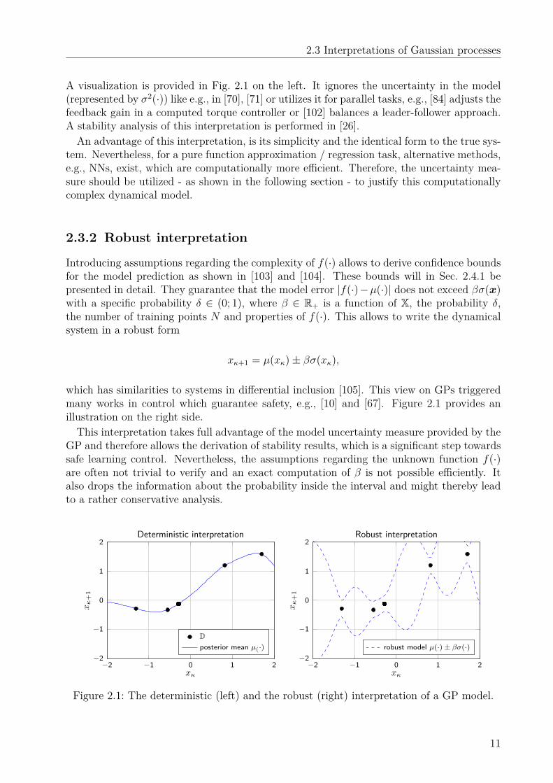
A visualization is provided in Fig. 2.1 on the left. It ignores the uncertainty in the model(represented by σ2(·)) like e.g., in [70], [71] or utilizes it for parallel tasks, e.g., [84] adjusts thefeedback gain in a computed torque controller or [102] balances a leader-follower approach.A stability analysis of this interpretation is performed in [26].An advantage of this interpretation, is its simplicity and the identical form to the true sys-
tem. Nevertheless, for a pure function approximation / regression task, alternative methods,e.g., NNs, exist, which are computationally more efficient. Therefore, the uncertainty mea-sure should be utilized - as shown in the following section - to justify this computationallycomplex dynamical model.
2.3.2 Robust interpretation
Introducing assumptions regarding the complexity of f(·) allows to derive confidence boundsfor the model prediction as shown in [103] and [104]. These bounds will in Sec. 2.4.1 bepresented in detail. They guarantee that the model error |f(·)−µ(·)| does not exceed βσ(x)with a specific probability δ ∈ (0; 1), where β ∈ R+ is a function of X, the probability δ,the number of training points N and properties of f(·). This allows to write the dynamicalsystem in a robust form
xκ+1 = µ(xκ)± βσ(xκ),
which has similarities to systems in differential inclusion [105]. This view on GPs triggeredmany works in control which guarantee safety, e.g., [10] and [67]. Figure 2.1 provides anillustration on the right side.This interpretation takes full advantage of the model uncertainty measure provided by the
GP and therefore allows the derivation of stability results, which is a significant step towardssafe learning control. Nevertheless, the assumptions regarding the unknown function f(·)are often not trivial to verify and an exact computation of β is not possible efficiently. Italso drops the information about the probability inside the interval and might thereby leadto a rather conservative analysis.
−2 −1 0 1 2−2
−1
0
1
2
xκ
xκ
+1
Deterministic interpretation
Dposterior mean µ(·)
−2 −1 0 1 2−2
−1
0
1
2
xκ
xκ
+1
Robust interpretation
robust model µ(·) ± βσ(·)
Figure 2.1: The deterministic (left) and the robust (right) interpretation of a GP model.
11
2 Gaussian Processes in Identification and Control
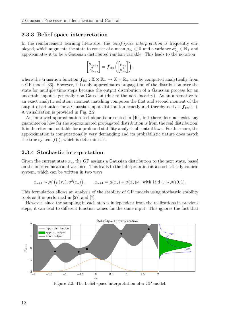
2.3.3 Belief-space interpretationIn the reinforcement learning literature, the belief-space interpretation is frequently em-ployed, which augments the state to consist of a mean µxκ ∈ X and a variance σ2
xκ ∈ R+ andapproximates it to be a Gaussian distributed random variable. This leads to the notation[
µxκ+1
σ2xκ+1
]= fBS
([µxκσ2xκ
]),
where the transition function fBS : X × R+ → X × R+ can be computed analytically froma GP model [33]. However, this only approximates propagation of the distribution over thestate for multiple time steps because the output distribution of a Gaussian process for anuncertain input is generally non-Gaussian (due to the non-linearity). As an alternative toan exact analytic solution, moment matching computes the first and second moment of theoutput distribution for a Gaussian input distribution exactly and thereby derives fBS(·, ·).A visualization is provided in Fig. 2.2.An improved approximation technique is presented in [40], but there does not exist any
guarantee on how far the approximated propagated distribution is from the real distribution.It is therefore not suitable for a profound stability analysis of control laws. Furthermore, theapproximation is computationally very demanding and its probabilistic nature does matchthe true system f(·), which is deterministic.
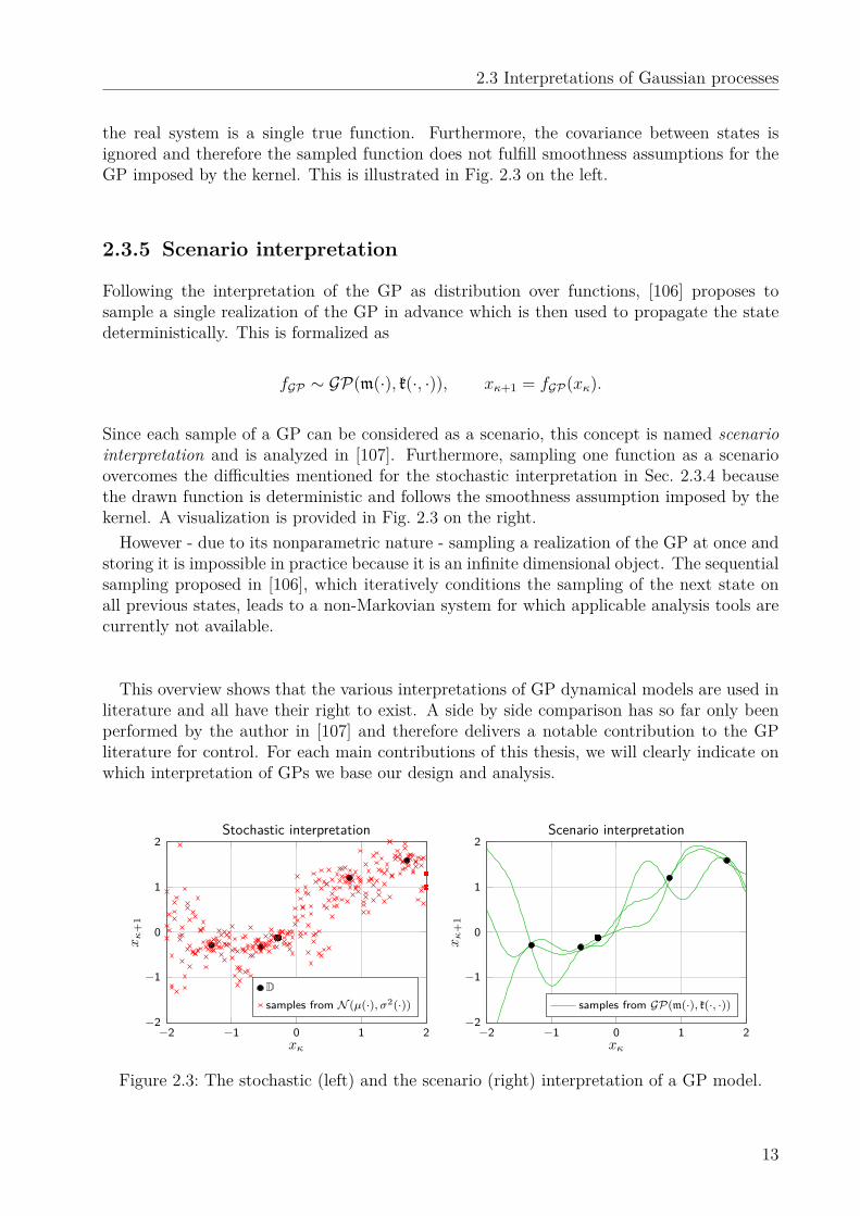
2.3.4 Stochastic interpretationGiven the current state xκ, the GP assigns a Gaussian distribution to the next state, basedon the inferred mean and variance. This leads to the interpretation as a stochastic dynamicalsystem, which can be written in two ways
xκ+1 ∼ N(µ(xκ),σ2(xκ)
), xκ+1 = µ(xκ) + σ(xκ)ω, with i.i.d ω ∼ N (0, 1).
This formulation allows an analysis of the stability of GP models using stochastic stabilitytools as it is performed in [27] and [7].However, since the sampling in each step is independent from the realizations in previous
steps, it can lead to different function values for the same input. This ignores the fact that
−2 −1.5 −1 −0.5 0 0.5 1 1.5 2−2
−1
0
1
2
xκ
xκ
+1
Belief-space interpretation
input distributionapprox. outputexact output
Figure 2.2: The belief-space interpretation of a GP model.
12
2.3 Interpretations of Gaussian processes
the real system is a single true function. Furthermore, the covariance between states isignored and therefore the sampled function does not fulfill smoothness assumptions for theGP imposed by the kernel. This is illustrated in Fig. 2.3 on the left.
2.3.5 Scenario interpretation
Following the interpretation of the GP as distribution over functions, [106] proposes tosample a single realization of the GP in advance which is then used to propagate the statedeterministically. This is formalized as
fGP ∼ GP(m(·), k(·, ·)), xκ+1 = fGP(xκ).
Since each sample of a GP can be considered as a scenario, this concept is named scenariointerpretation and is analyzed in [107]. Furthermore, sampling one function as a scenarioovercomes the difficulties mentioned for the stochastic interpretation in Sec. 2.3.4 becausethe drawn function is deterministic and follows the smoothness assumption imposed by thekernel. A visualization is provided in Fig. 2.3 on the right.However - due to its nonparametric nature - sampling a realization of the GP at once and
storing it is impossible in practice because it is an infinite dimensional object. The sequentialsampling proposed in [106], which iteratively conditions the sampling of the next state onall previous states, leads to a non-Markovian system for which applicable analysis tools arecurrently not available.
This overview shows that the various interpretations of GP dynamical models are used inliterature and all have their right to exist. A side by side comparison has so far only beenperformed by the author in [107] and therefore delivers a notable contribution to the GPliterature for control. For each main contributions of this thesis, we will clearly indicate onwhich interpretation of GPs we base our design and analysis.
−2 −1 0 1 2−2
−1
0
1
2
xκ
xκ
+1
Stochastic interpretation
Dsamples from N (µ(·), σ2(·))
−2 −1 0 1 2−2
−1
0
1
2
xκ
xκ
+1
Scenario interpretation
samples from GP(m(·), k(·, ·))
Figure 2.3: The stochastic (left) and the scenario (right) interpretation of a GP model.
13
2 Gaussian Processes in Identification and Control
2.4 Properties and bounds for Gaussian processesGaussian processes are well researched and there exist numerous literature on their propertiesfrom the fields of machine learning, statistics and information theory. However, only a fewresults are relevant for this thesis, which are reviewed in the following.
2.4.1 Error bounds for Gaussian process modelsGaussian processes are particularly appealing for applications in control of safety-criticalsystems because a formal analysis is analytically possible. As mentioned in Sec. 2.3.2, it ispossible to bound the error between the posterior mean function µ(·) and the function f(·)of which the measurements are taken with high probability. However, such a guarantee doesnot come without any assumptions on f(·) as the no-free-lunch theorem suggest [108].The assumption does - thanks to the nonparametric nature of the GP - not require any
structural knowledge on f(·), like parametric regression techniques do. But it limits thecomplexity of the function as measured by the reproducing kernel Hilbert space (RKHS) asformulated in the following.
Assumption 2.1. The function f : X → R has a bounded RKHS norm with respect to aknown kernel k(·, ·), denoted by ‖f(·)‖2
k ≤ Bf .
A RKHS is a complete subspace of the L2, for which the inner product 〈·, ·〉k fulfills thereproducing property 〈f , k(x, ·)〉k = f(x). The induced norm ‖f‖k =
√〈f , f〉k measures the
smoothness of f(·). In most cases (for universal differentiable kernels), Assumption 2.1translates in practice to assuming a continuously differentiable dynamic behavior. Thisexcludes for example impacts which lead to switching dynamics e.g. a bouncing ball orrobotic interaction tasks.Furthermore the information gain which can be obtained on a compact set X from N + 1
noisy measurements x(1), . . . ,x(N+1) is defined as
γ = maxx(1:N+1)∈X
12 log det
(IN+1 + 1
σ2onK
), with K = k
(x(1:N+1),x(1:N+1)
). (2.9)
This allows to derive a bound for the model error as following.
Theorem 2.1. Consider a compact set X ⊂ Rn, a function f : X→ R under Assumption 2.1and a probability δ ∈ (0; 1). Then,
P |µ(x)− f(x)| ≤ βσ(x),∀x ∈ X,N ∈ N0 ≥ 1− δ, (2.10)
where β =√
2Bf + 300γ log3((N + 1)/δ) and µ(·), σ(·) are posterior mean / variance func-tion of a GP for N data points as defined in (2.4)
Proof. This result is stated and proven in [104, Theorem 6]1
1The constant 300 is not the exact number as it results from the derivation of the bound but is utilized bythe authors of [104] as conservative abbreviation of a constant factor for notational convenience.
14
2.4 Properties and bounds for Gaussian processes
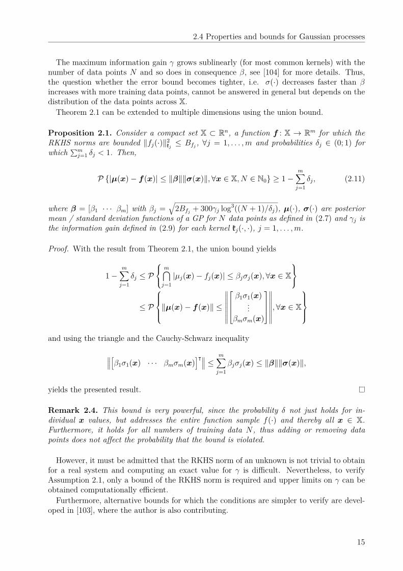
The maximum information gain γ grows sublinearly (for most common kernels) with thenumber of data points N and so does in consequence β, see [104] for more details. Thus,the question whether the error bound becomes tighter, i.e. σ(·) decreases faster than βincreases with more training data points, cannot be answered in general but depends on thedistribution of the data points across X.Theorem 2.1 can be extended to multiple dimensions using the union bound.
Proposition 2.1. Consider a compact set X ⊂ Rn, a function f : X → Rm for which theRKHS norms are bounded ‖fj(·)‖2
kj≤ Bfj , ∀j = 1, . . . ,m and probabilities δj ∈ (0; 1) for
which ∑mj=1 δj < 1. Then,
P |µ(x)− f(x)| ≤ ‖β‖‖σ(x)‖,∀x ∈ X,N ∈ N0 ≥ 1−m∑j=1
δj, (2.11)
where β = [β1 · · · βm] with βj =√
2Bfj + 300γj log3((N + 1)/δj), µ(·), σ(·) are posteriormean / standard deviation functions of a GP for N data points as defined in (2.7) and γj isthe information gain defined in (2.9) for each kernel kj(·, ·), j = 1, . . . ,m.
Proof. With the result from Theorem 2.1, the union bound yields
1−m∑j=1
δj ≤ P
m⋂j=1|µj(x)− fj(x)| ≤ βjσj(x),∀x ∈ X
≤ P
‖µ(x)− f(x)‖ ≤
∥∥∥∥∥∥∥∥β1σ1(x)
...βmσm(x)
∥∥∥∥∥∥∥∥,∀x ∈ X
and using the triangle and the Cauchy-Schwarz inequality
∥∥∥[β1σ1(x) · · · βmσm(x)]ᵀ∥∥∥ ≤ m∑
j=1βjσj(x) ≤ ‖β‖‖σ(x)‖,
yields the presented result.
Remark 2.4. This bound is very powerful, since the probability δ not just holds for in-dividual x values, but addresses the entire function sample f(·) and thereby all x ∈ X.Furthermore, it holds for all numbers of training data N , thus adding or removing datapoints does not affect the probability that the bound is violated.
However, it must be admitted that the RKHS norm of an unknown is not trivial to obtainfor a real system and computing an exact value for γ is difficult. Nevertheless, to verifyAssumption 2.1, only a bound of the RKHS norm is required and upper limits on γ can beobtained computationally efficient.Furthermore, alternative bounds for which the conditions are simpler to verify are devel-
oped in [103], where the author is also contributing.
15
2 Gaussian Processes in Identification and Control
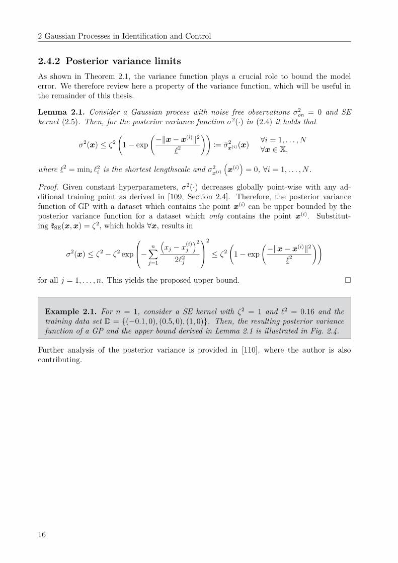
2.4.2 Posterior variance limitsAs shown in Theorem 2.1, the variance function plays a crucial role to bound the modelerror. We therefore review here a property of the variance function, which will be useful inthe remainder of this thesis.
Lemma 2.1. Consider a Gaussian process with noise free observations σ2on = 0 and SE
kernel (2.5). Then, for the posterior variance function σ2(·) in (2.4) it holds that
σ2(x) ≤ ζ2(
1− exp(−‖x− x(i)‖2
`2
)):= σ2
x(i)(x) ∀i = 1, . . . ,N∀x ∈ X,
where `2 = mini `2i is the shortest lengthscale and σ2
x(i)
(x(i)
)= 0, ∀i = 1, . . . ,N .
Proof. Given constant hyperparameters, σ2(·) decreases globally point-wise with any ad-ditional training point as derived in [109, Section 2.4]. Therefore, the posterior variancefunction of GP with a dataset which contains the point x(i) can be upper bounded by theposterior variance function for a dataset which only contains the point x(i). Substitut-ing kSE(x,x) = ζ2, which holds ∀x, results in
σ2(x) ≤ ζ2 − ζ2 exp
− n∑j=1
(xj − x(i)
j
)2
2`2j
2
≤ ζ2(
1− exp(−‖x− x(i)‖2
`2
))
for all j = 1, . . . ,n. This yields the proposed upper bound.
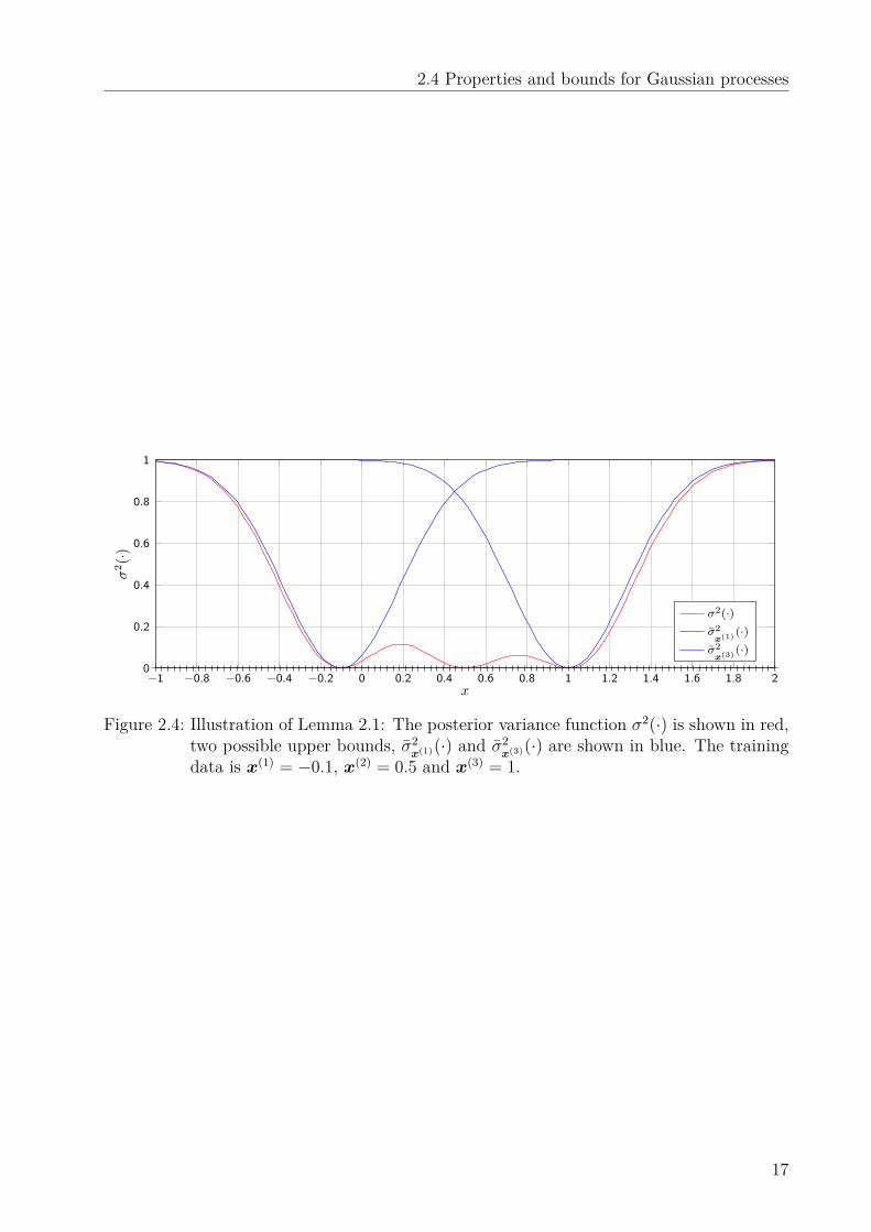
Example 2.1. For n = 1, consider a SE kernel with ζ2 = 1 and `2 = 0.16 and thetraining data set D = (−0.1, 0), (0.5, 0), (1, 0). Then, the resulting posterior variancefunction of a GP and the upper bound derived in Lemma 2.1 is illustrated in Fig. 2.4.
Further analysis of the posterior variance is provided in [110], where the author is alsocontributing.
16
2.4 Properties and bounds for Gaussian processes
−1 −0.8 −0.6 −0.4 −0.2 0 0.2 0.4 0.6 0.8 1 1.2 1.4 1.6 1.8 20
0.2
0.4
0.6
0.8
1
x
σ2 (
·)
σ2(·)σ2
x(1) (·)σ2
x(3) (·)
Figure 2.4: Illustration of Lemma 2.1: The posterior variance function σ2(·) is shown in red,two possible upper bounds, σ2
x(1)(·) and σ2x(3)(·) are shown in blue. The training
data is x(1) = −0.1, x(2) = 0.5 and x(3) = 1.
17

Identification of Stable Systems 3
Data-driven modeling techniques are very powerful for systems where no analytic modelcan be derived. However, the lack of an analytic description does not imply that no priorknowledge about the system is given. In particular, for many physical systems, so calledhigh-level knowledge is accessible, e.g., balance of in and out flow in a node, smoothnessof the dynamics or the energy dissipation [111]. These fundamental properties are oftennot considered in data-driven modeling and the resulting models thereby make physicallyinconsistent predictions.This work focuses on the consistent energy dissipation between the true system and the
data-driven model, which is closely entangled with the convergence behavior of a dynamicalsystem. Utilizing such high-level prior knowledge is not only helpful for increasing the modelprecision but also crucial as without any prior knowledge no generalization outside of thetraining points can be expected (see no-free-lunch theorems [108]).The presented techniques can not only be employed for physically consistent modeling,
but are also applicable in human-like motion generation: Assume a goal-directed humanmovement is modeled by a dynamical system in a robotic learning by demonstration scenario.Then, the training data converges to the desired goal point and this behavior must alsobe represented by the model. Thus, the model must represent the demonstrated motionaccurately and ensure that all generated trajectories converge to the goal point.Ensuring physically consistent prediction or stability of a parametric model is rather
simple to verify, see [112] and [113]. Other classical system identification techniques, e.g.autoregressive–moving-average (ARMA) models rely on subspace methods to ensure stabil-ity [114], [115]. The deconvolution problem, to find the impulse response given input-outputdata, is approached using regularization techniques as discussed in [116] and recent overviewsare given in [117] and [118]. This problem is also considered by the machine learning com-munity using kernel-based techniques to identify the impulse response, see [119] and [120].For the nonlinear case, Volterra series or Wiener-Hammerstein models exist, which con-
sider a very limited structure of the model [16]. Therefore, supervised learning methods,e.g., NNs [121] or GPSSMs have gained attention, see [122] and [21]. However, an analysisof the system stability is missing in these studies. A first GPSSM stability analysis is per-formed in [26] and [27], for the deterministic and the stochastic interpretation, respectively.Enforcing stability to Gaussian mixture models (GMMs) is studied in [123] and [124] andmore general techniques are developed in [125], [126] and [127].While these approaches aim to incorporate stability into a model, none of them deals
with the inherent challenge of data-driven approaches that data is usually sparse and theresulting models are imprecise. The uncertainty resulting from finite data is commonlyignored. Therefore, this chapter develops a framework to deal with these uncertainties
19
3 Identification of Stable Systems
in form of a stochastic dynamical system and ensures its asymptotic convergence usingstochastic stability theory [128].The main contribution is a novel identification algorithm to learn asymptotically stable
GPSSMs using control Lyapunov functions. For the deterministic interpretation of the GP,we show a realization for arbitrary datasets and prove that the model is improved throughthe stabilization. For the stochastic interpretation, we derive conditions for almost sureasymptotic convergence and show how many additional training data are required to ensureasymptotic stability if these conditions are not fulfilled on the initial dataset. To learn theconvergence behavior in a data-driven fashion, we propose the use of a sum of squares (SOS)control Lyapunov function. This allows a computationally efficient estimation of unknownequilibria and we demonstrate its advantages in simulation over alternative Lyapunov can-didates on a real-world dataset.The chapter is based on the work published in [7] and [8]. It is structured as follows: After
defining the problem setting in Sec. 3.1, this chapter proposes in Sec. 3.2 an optimization-based stabilization of a GPSSM for the deterministic and the stochastic interpretation (asintroduced in Sec. 2.3). A data-driven search for a suitable control Lyapunov functionis presented in Sec. 3.3 followed by a numerical evaluation in Sec. 3.4 and a discussionin Sec. 3.5.
3.1 Problem formulationHere, we consider an unknown discrete-time system with state x ∈ X ⊆ Rn, n ∈ N, given by
xκ+1 = f(xκ), (3.1)
with initial condition x0 ∈ X, where κ ∈ N and f : X→ X. The following is assumed.
Assumption 3.1. The function f(·) is continuously differentiable but unknown.
Remark 3.1. The smoothness of the function f(·) is a quite natural assumption and holdsfor a large class of systems. It is also an essential one because the generalization outside ofa training data set becomes very difficult for discontinuous functions [108].
The available training data set is assumed to take the following form
Assumption 3.2. The training set of N data pairs consists of consecutive measurements ofthe state
D =(x(i),y(i)
)Ni=1
,
where y(i) = x(i)κ+1 is the consecutive state to x(i)
κ .1
Remark 3.2. The data does not necessarily stem from a single trajectory. Each pair canbe taken independently from other pairs and the order in the training set is not decisive. Avisualization of a possible data set is provided in Fig. 3.1
Furthermore, we make an assumption on the asymptotic behavior of the system (3.1).1An extension to noisy measurements of the consecutive state is directly possible. However, we considerit as an unrealistic setting to have noise on the consecutive state but not on the current state (as theformer becomes the latter in the next time step).
20
3.1 Problem formulation
x1
x2
x1∗ x(1)
y(1)x(2)
y(2)
x(3)
y(3)
x2∗ x(4)
y(4)
x(5)
y(5)
x(6)y(6)
x(7)y(7)
x(8)
y(8)
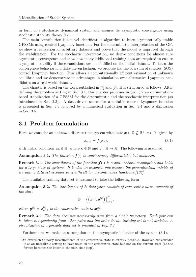
Figure 3.1: An illustration of a training dataset D with two equilibria x1∗ ,x2∗ . The data origi-nate from three different trajectories (1-2-3,4-5-6,7-8). Within one trajectory, theend point of one step is the starting point of the next, e.g., y(1) = x(2), y(4) = x(5),etc., but this is not necessarily the case.
Assumption 3.3. There exist N∗ unknown equilibria, denoted as xi∗ ∈ Xi∗ ⊆ X, wherei∗ = 1, . . . ,N∗ and f(xi∗) = xi∗. Each of the equilibria is asymptotically stable with corre-sponding known domain of attraction Xi∗ ⊆ X for which holds
Xi∗ ∩ Xi′∗ = ∅, ∀i′∗ 6= i∗, andN∗⋃i∗=1
Xi∗ = X.
This formulates the main motivation of this chapter. A physical system whose dynamicsare unknown, dissipates energy and will eventually reach an equilibrium point. This equilib-rium is not known and it is also tedious to determine it experimentally (since it takes usuallyinfinite time to be reached). In contrast, the region of attraction is commonly easier to find.
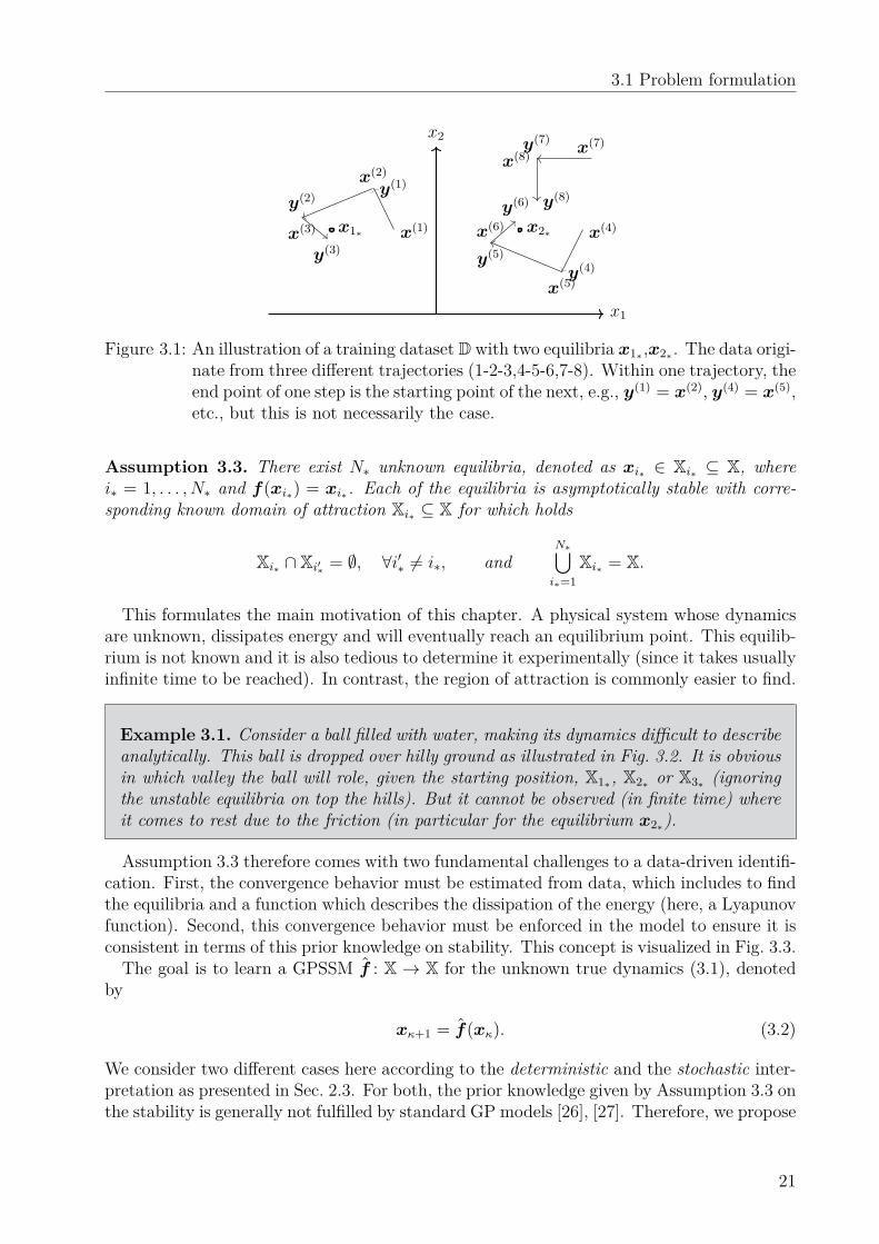
Example 3.1. Consider a ball filled with water, making its dynamics difficult to describeanalytically. This ball is dropped over hilly ground as illustrated in Fig. 3.2. It is obviousin which valley the ball will role, given the starting position, X1∗, X2∗ or X3∗ (ignoringthe unstable equilibria on top the hills). But it cannot be observed (in finite time) whereit comes to rest due to the friction (in particular for the equilibrium x2∗).
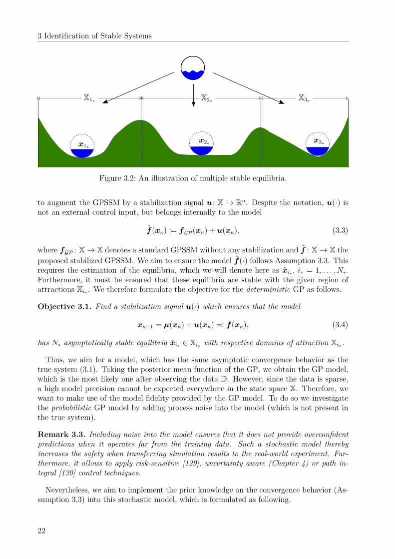
Assumption 3.3 therefore comes with two fundamental challenges to a data-driven identifi-cation. First, the convergence behavior must be estimated from data, which includes to findthe equilibria and a function which describes the dissipation of the energy (here, a Lyapunovfunction). Second, this convergence behavior must be enforced in the model to ensure it isconsistent in terms of this prior knowledge on stability. This concept is visualized in Fig. 3.3.The goal is to learn a GPSSM f : X → X for the unknown true dynamics (3.1), denoted
by
xκ+1 = f(xκ). (3.2)
We consider two different cases here according to the deterministic and the stochastic inter-pretation as presented in Sec. 2.3. For both, the prior knowledge given by Assumption 3.3 onthe stability is generally not fulfilled by standard GP models [26], [27]. Therefore, we propose
21
3 Identification of Stable Systems
X1∗ X2∗ X3∗
x1∗x2∗ x3∗
Figure 3.2: An illustration of multiple stable equilibria.
to augment the GPSSM by a stabilization signal u : X → Rn. Despite the notation, u(·) isnot an external control input, but belongs internally to the model
f(xκ) := fGP(xκ) + u(xκ), (3.3)
where fGP : X→ X denotes a standard GPSSM without any stabilization and f : X→ X theproposed stabilized GPSSM. We aim to ensure the model f(·) follows Assumption 3.3. Thisrequires the estimation of the equilibria, which we will denote here as xi∗ , i∗ = 1, . . . ,N∗.Furthermore, it must be ensured that these equilibria are stable with the given region ofattractions Xi∗ . We therefore formulate the objective for the deterministic GP as follows.
Objective 3.1. Find a stabilization signal u(·) which ensures that the model
xκ+1 = µ(xκ) + u(xκ) =: f(xκ), (3.4)
has N∗ asymptotically stable equilibria xi∗ ∈ Xi∗ with respective domains of attraction Xi∗.
Thus, we aim for a model, which has the same asymptotic convergence behavior as thetrue system (3.1). Taking the posterior mean function of the GP, we obtain the GP model,which is the most likely one after observing the data D. However, since the data is sparse,a high model precision cannot be expected everywhere in the state space X. Therefore, wewant to make use of the model fidelity provided by the GP model. To do so we investigatethe probabilistic GP model by adding process noise into the model (which is not present inthe true system).
Remark 3.3. Including noise into the model ensures that it does not provide overconfidentpredictions when it operates far from the training data. Such a stochastic model therebyincreases the safety when transferring simulation results to the real-world experiment. Fur-thermore, it allows to apply risk-sensitive [129], uncertainty aware (Chapter 4) or path in-tegral [130] control techniques.
Nevertheless, we aim to implement the prior knowledge on the convergence behavior (As-sumption 3.3) into this stochastic model, which is formulated as following.
22
3.2 Stabilized Gaussian process state space models
data
estimating convergence
behavior (Sec. 3.3)
estimating dynamic
behavior (Sec. 2.1)
Lyapunovfunction
equilibriumpoints
virtual stabiliser(Sec. 3.2.1 & 3.2.2)
stabilizedGPSSMrequest more data (Sec. 3.2.3)
Figure 3.3: An overview of the proposed scheme for a data-driven stabilization of GPSSMs.
Objective 3.2. Find a stabilization signal u(·) such that the model
xκ+1 = µ(xκ) + u(xκ) +√
Σ(xκ)ωκ = f(xκ) +√
Σ(xκ)ωκ ωκ ∼ N (0, In), (3.5)
has N∗ almost surely (a.s.) asymptotically stable equilibria xi∗ ∈ Xi∗, i∗ = 1, . . . ,N∗. Thus,for all x0 ∈ Xi∗ it holds that
limk→∞P(‖xκ − xi∗‖ = 0) = 1, ∀i∗ = 1, . . . ,N∗. (3.6)
The i.i.d. random variable ωκ ∈ Rn originates from the probability space (Ω,F ,P), whichhas the sample space Ω = Rn and the sigma-algebra F of Borel sets on Ω. The probabilitymeasure P is a normal distribution.This chapter presents an algorithm which fulfills Objectives 3.1 and 3.2 using the aug-
mented GP model (3.3).
3.2 Stabilized Gaussian process state space modelsIn this section, we elaborate how stability of a GPSSM is enforced with the stabilizationsignal u(·) using a given control Lyapunov function.The first step towards Objectives 3.1 and 3.2 is to ensure that the GP mean function
estimate µ(·) has a fixed point at the given equilibria estimates xi∗ , thus xi∗ = µ(xi∗) forall i∗ = 1, . . . ,N∗. This can be achieved as described in Remark 2.3, and will therefore notfurther be discussed here. However, this will not ensure the asymptotic stability of theseequilibria or ensure the proper domain of attraction. To make the convergence behavior ofthe model match the true system, this section discusses the choice of the internal stabilizingsignal u ∈ Rn in f(x).We assume to be given N∗ control Lyapunov functions V i∗
θi∗: X → R+,0 which are all
parameterized by θi∗ ∈ Θi∗ ⊆ Rnθi , nθi ∈ N and an estimated equilibrium xi∗ ∈ Xi∗ (seeSec. 3.3 how the parameters are obtained from data). The following assumptions are made.
Assumption 3.4. For all parameter choices θi∗ ∈ Θi∗, the functions V i∗θi∗
(·) are continuousand positive definite, thus
V i∗θi∗
(x) > 0, ∀x ∈ X\xi∗ and V i∗θi∗
(xi∗) = 0, ∀i∗ = 1, . . . ,N∗.
23
3 Identification of Stable Systems
Assumption 3.5. The functions V i∗θi∗
(·) are radially unbounded
lim‖x−xi∗‖→∞
V i∗θi∗
(x) =∞, ∀θi∗ ∈ Θi∗ .
These assumptions make V i∗θi∗
(·) Lyapunov candidates. We consider the deterministicinterpretation of the GP first in Sec. 3.2.1 before dealing with the stochastic interpretationin Sec. 3.2.2 and 3.2.3.
3.2.1 Deterministic interpretationFor the deterministic interpretation of a GPSSM, the next state, given the current state, isobtained from xκ+1 = µ(xκ). Using Remark 2.3 the estimated equilibria are incorporated,but their asymptotic stability is not ensured. Therefore, the following optimization-basedstabilization is proposed.
Theorem 3.1. Consider the GP (2.7)/ (2.8) with SE kernel (2.5) and the stabilizing com-mand u∗(·) obtained from the optimization
u∗(xκ) = arg minu
12u
ᵀu, (3.7a)
s.t. V i∗θi∗
(µ(xκ) + u)− V i∗θi∗
(xκ) < 0 if xκ 6= xi∗ ,and u = 0 if xκ = xi∗ ,
(3.7b)
where i∗ is chosen such that x0 ∈ Xi∗ and V i∗θi∗
(·) is a Lyapunov candidate which fulfillsAssumption 3.4. Then, the model
xκ+1 = f(xκ) = µ(xκ) + u∗(xκ), (3.8)
converges asymptotically to the equilibrium xi∗ for all x0 ∈ Xi∗.
Proof. The optimization (3.7) ensures that the Lyapunov function V i∗θi∗
(·) decreases in everystep V i∗
θi∗(f(xκ))− V i∗
θi∗(xκ) < 0, ∀xκ ∈ X \ xi∗. The constraint set is not empty ∀xκ ∈ X,
since a feasible solution u = xi∗−µ(xi∗) always exists with V i∗θi∗
(xi∗)− V i∗θi∗
(xκ) = −V i∗θi∗
(xκ)being negative definite.
An illustration of this optimization-based stabilization is provided in Fig. 3.4 on the leftside. For a single equilibrium point, this result can directly be extended to global stability.
Corollary 3.1. Let N∗ = 1, Vθ(·) is radially unbounded (Assumption 3.5), and X = Rn. Fur-thermore, consider a GP (2.7)/ (2.8) with SE kernel (2.5) and the stabilizing command u∗(·)proposed in (3.7). Then, the equilibrium x∗ of the model (3.8) is globally asymptoticallystable (GAS).
Proof. Since the Lyapunov function is radially unbounded and decreasing over time (compareTheorem 3.1) the necessary conditions for global stability hold [131].
Thus, with the optimization-based choice in (3.7), Objective 3.1 is achieved.
24
3.2 Stabilized Gaussian process state space models
Remark 3.4. There are many choices for u(·) which would fulfill Objective 3.1 and themost trivial is u = xi∗ − µ(xi∗). However, we are not just trying to stabilize the model, butwe aim to replicate the true system (3.1) as precise as possible. Therefore the GPSSM µ(·)should be distorted only minimally because it represents the data optimal (according to thelikelihood optimization).
It can be shown that (for a convex Lyapunov function) the GPSSM without stabiliza-tion µ(·) performs never better - in terms of prediction precision - than the proposed stabi-lized GPSSM f(·) = µ(·) + u(·).
Proposition 3.1. Consider the GP (2.7)/ (2.8) with SE kernel (2.5) and convex Lyapunovfunctions V i∗
θi∗(·) which fulfill Assumption 3.4 and V i∗
θi∗(f(x))−V i∗
θi∗(x) < 0, ∀x ∈ Xi∗ \xi∗,
and ∀i∗. Then, the prediction error of the GPSSM without stabilization µ(·) is never smallerthan that of the stabilized GPSSM f(·), thus
‖f(xκ)− f(xκ)‖ ≤ ‖µ(xκ)− f(xκ)‖, ∀xκ ∈ X. (3.9)
Proof. Since the true system (3.1) is asymptotically stable (Assumption 3.3), the Lya-punov function V i∗
θi∗(·) decreases with every step. Thus the next step f(xκ) lies within
the set Vxκ =x ∈ X
∣∣∣V i∗θi∗
(x) < V i∗θi∗
(xκ), which is convex due to the convexity of V i∗
θi∗(·).
For all xκ for which µ(xκ) ∈ Vxκ , holds u(xκ) = 0 and thus f(xκ) = µ(xκ), which resultsin equality in (3.9). For all xκ for which µ(xκ) /∈ Vxκ , the stabilized GPSSM f(xκ) resultsin a projection onto the convex set Vxκ , thus
f(xκ) = minxκ+1∈Vxκ
‖xκ+1 − µ(xκ)‖.
The projection f(xκ) is closer to any point in the convex set Vxκ than µ(xκ). Therefore, itis also closer to f(xκ).
Remark 3.5. Consider that Proposition 3.1 implies the assumption, that V i∗θi∗
(·) are Lya-punov functions of the unknown system. These are typically unknown and therefore thisimposes a quite strict assumption.
For an infinite number of training points, it can be shown that the proposed model (3.8)converges to the true system.
Proposition 3.2. Consider the GP (2.7)/ (2.8) on a compact set X ⊂ Rn with SE ker-nel (2.5) and Lyapunov functions V i∗
θi∗(·) which fulfill Assumption 3.4 and the condition
V i∗θi∗
(f(x))−V i∗θi∗
(x) < 0, for all x ∈ X \ xi∗, ∀i∗. Let f(·) be a sample from the GP fromwhich infinitely many training points are generated using a dense distribution on X, then themodel f(·) approaches the true system f(·) almost surely
P
limN→∞
supx∈X
∥∥∥f(xκ)− f(xκ)∥∥∥ = 0
= 1
for a stabilizing command u∗(xκ) = 0 ∀xκ ∈ X.
25
3 Identification of Stable Systems
Proof. Under the specified conditions, the maximum difference between the mean func-tion µ(·) and the true function f(·) becomes arbitrarily small almost surely. This is awell established result from scattered data interpolation [132, Eq. 2.11], where the error isbounded by a power function (which corresponds to the posterior standard deviation of aGP [133, Sec. 5.2]). This converges to zero for N →∞ [110, Corollary 3.2.]. Since V i∗
θi∗(·) is
a continuous function the condition
V i∗θi∗
(µ(xκ))− V i∗θi∗
(xκ) < 0, ∀xκ ∈ X \ xi∗
is fulfilled in the limitN →∞, and therefore u∗(xκ) = 0, ∀xκ ∈ X, which yields the providedresult.
This result uses simply the fact that a GP converges to the function from which the datais taken. In this case, the stabilization becomes inactive and therefore does not distort themodel.Regarding the optimization (3.7), the following is concluded.
Proposition 3.3. The optimization problem (3.7) is convex if and only if V i∗θi∗
(x) is convex.
Proof. In the definition of the constraint set (3.7b), µ(xκ) and V i∗θi∗
(xκ) are constant withrespect to the optimization variable u. The addition of u preserves the convexity. Therefore,the constraint set is convex if and only if V i∗
θi∗(·) is convex, which results in convexity of the
optimization problem as defined in [134].
This allows to employ efficient solvers for the optimization (3.7) in case of convex Lyapunovfunctions.
Remark 3.6. For non-convex Lyapunov functions, finding a global minimum efficientlycannot be expected. Nevertheless, the stability of the model (Theorem 3.1) is not affected,because any feasible u results in a stable system. Suboptimal solutions will only potentiallyresult in behavior different from the training data, but convergence remains guaranteed.This also facilitates the implementation in real-time critical applications: Since the opti-
mization is initialized at a feasible (i.e. stability guaranteeing) value, the optimization canbe interrupted at any time without affecting the convergence (assuming the solver stays inthe feasible region).
3.2.2 Probabilistic interpretationFor the probabilistic interpretation, the GPSSM infers a Gaussian distribution over the nextstate given the current state as it is formalized in (3.5). The resulting system is analyzedusing tools from stochastic dynamical systems as reviewed in the following.
Lemma 3.1 (Stability of stochastic systems [135]). Consider a system of the form (3.5). Ifthere exists a positive definite function V : X→ R+,0 for which holds
E[V (xκ+1)|xκ]− V (xκ) < 0, ∀xκ ∈ X \ x∗, (3.10)
26
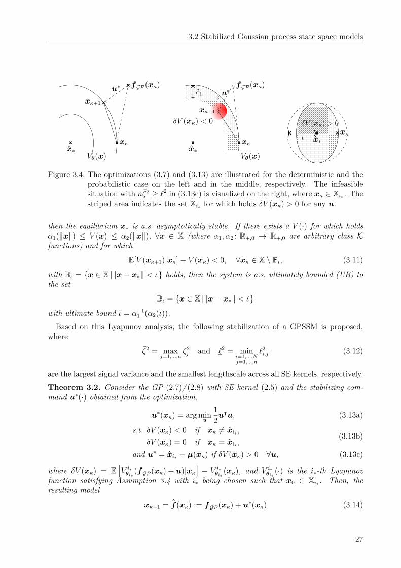
3.2 Stabilized Gaussian process state space models
Vθ(x)
xκ
fGP(xκ)
x∗
xκ+1
u∗ c1
Vθ(x)
xκ
fGP(xκ)
x∗
δV (xκ) < 0xκ+1
u∗
δV (xκ) > 0
x∗ιxκ
Figure 3.4: The optimizations (3.7) and (3.13) are illustrated for the deterministic and theprobabilistic case on the left and in the middle, respectively. The infeasiblesituation with nζ2 ≥ `2 in (3.13c) is visualized on the right, where xκ ∈ Xi∗ . Thestriped area indicates the set Xi∗ for which holds δV (xκ) > 0 for any u.
then the equilibrium x∗ is a.s. asymptotically stable. If there exists a V (·) for which holdsα1(‖x‖) ≤ V (x) ≤ α2(‖x‖), ∀x ∈ X (where α1,α2 : R+,0 → R+,0 are arbitrary class Kfunctions) and for which
E[V (xκ+1)|xκ]− V (xκ) < 0, ∀xκ ∈ X \ Bι, (3.11)
with Bι = x ∈ X |‖x− x∗‖ < ι holds, then the system is a.s. ultimately bounded (UB) tothe set
Bι = x ∈ X |‖x− x∗‖ < ιwith ultimate bound ι = α−1
1 (α2(ι)).Based on this Lyapunov analysis, the following stabilization of a GPSSM is proposed,
where
ζ2 = maxj=1,...,n
ζ2j and `2 = min
i=1,...,Nj=1,...,n
`2i,j (3.12)
are the largest signal variance and the smallest lengthscale across all SE kernels, respectively.Theorem 3.2. Consider the GP (2.7)/ (2.8) with SE kernel (2.5) and the stabilizing com-mand u∗(·) obtained from the optimization,
u∗(xκ) = arg minu
12u
ᵀu, (3.13a)
s.t. δV (xκ) < 0 if xκ 6= xi∗ ,δV (xκ) = 0 if xκ = xi∗ ,
(3.13b)
and u∗ = xi∗ − µ(xκ) if δV (xκ) > 0 ∀u, (3.13c)
where δV (xκ) = E[V i∗θi∗
(fGP(xκ) + u)|xκ]− V i∗
θi∗(xκ), and V i∗
θi∗(·) is the i∗-th Lyapunov
function satisfying Assumption 3.4 with i∗ being chosen such that x0 ∈ Xi∗. Then, theresulting model
xκ+1 = f(xκ) := fGP(xκ) + u∗(xκ) (3.14)
27
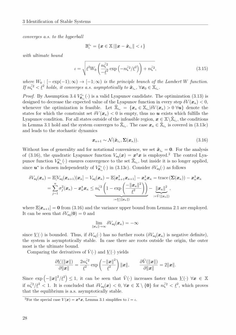
3 Identification of Stable Systems
converges a.s. to the hyperball
Bi∗ι = x ∈ X |‖x− xi∗‖ < ι
with ultimate bound
ι =
√√√√`2W0
(nζ2
−`2 exp(−nζ2/`2
))+ nζ2, (3.15)
where W0 : [− exp(−1);∞) → [−1;∞) is the principle branch of the Lambert W function.If nζ2 < `2 holds, it converges a.s. asymptotically to xi∗, ∀x0 ∈ Xi∗.
Proof. By Assumption 3.4 V i∗θi∗
(·) is a valid Lyapunov candidate. The optimization (3.13) isdesigned to decrease the expected value of the Lyapunov function in every step δV (xκ) < 0,whenever the optimization is feasible. Let Xi∗ = xκ ∈ Xi∗ |δV (xκ) > 0 ∀u denote thestates for which the constraint set δV (xκ) < 0 is empty, thus no u exists which fulfills theLyapunov condition. For all states outside of the infeasible region, x ∈ X\Xi∗ , the conditionsin Lemma 3.1 hold and the system converges to Xi∗ . The case xκ ∈ Xi∗ is covered in (3.13c)and leads to the stochastic dynamics
xκ+1 ∼ N (xi∗ , Σ(xκ)). (3.16)
Without loss of generality and for notational convenience, we set xi∗ = 0. For the analysisof (3.16), the quadratic Lyapunov function Vsq(x) = xᵀx is employed.2 The control Lya-punov function V i∗
θi∗(·) ensures convergence to the set Xi∗ , but inside it is no longer applied,
since u∗ is chosen independently of V i∗θi∗
(·) in (3.13c). Consider δVsq(·) as follows
δVsq(xκ) = E[Vsq(xκ+1)|xκ]− Vsq(xκ) = E[xᵀκ+1xκ+1]− xᵀ
κxκ = trace (Σ(xκ))− xᵀκxκ
=n∑j=1
σ2j (xκ)− xᵀ
κxκ ≤ nζ2(
1− exp(−‖xκ‖2
`2
))︸ ︷︷ ︸
:=V (‖xκ‖)
− ‖xκ‖2︸ ︷︷ ︸:=V (‖xκ‖)
,
where E[xκ+1] = 0 from (3.16) and the variance upper bound from Lemma 2.1 are employed.It can be seen that δVsq(0) = 0 and
lim‖xκ‖→∞
δVsq(xκ) = −∞
since V (·) is bounded. Thus, if δVsq(·) has no further roots (δVsq(xκ) is negative definite),the system is asymptotically stable. In case there are roots outside the origin, the outermost is the ultimate bound.Comparing the derivatives of V (·) and V (·) yields
∂V (‖x‖)∂‖x‖ = 2nζ2
`2 exp(−‖x‖2
`2
)‖x‖, ∂V (‖x‖)
∂‖x‖ = 2‖x‖.
Since exp(−‖x‖2/`2
)≤ 1, it can be seen that V (·) increases faster than V (·) ∀x ∈ X
if nζ2/`2 < 1. It is concluded that δVsq(x) < 0, ∀x ∈ X \ 0 for nζ2 < `2, which provesthat the equilibrium is a.s. asymptotically stable.
2For the special case V (x) = xᵀx, Lemma 3.1 simplifies to ι = ι.
28
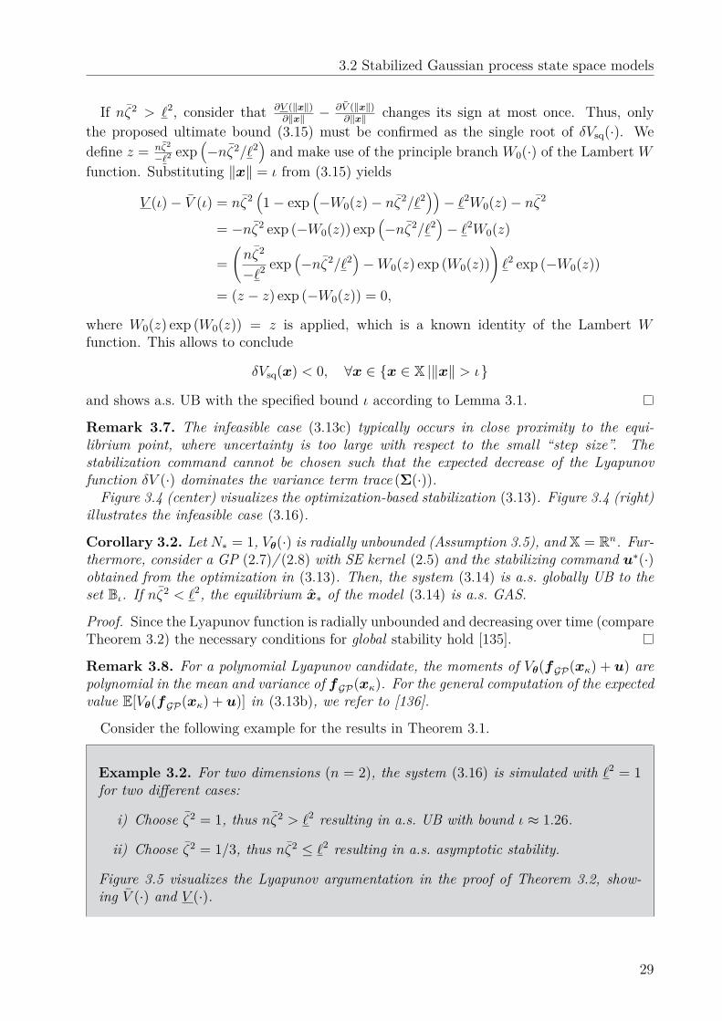
3.2 Stabilized Gaussian process state space models
If nζ2 > `2, consider that ∂V (‖x‖)∂‖x‖ −
∂V (‖x‖)∂‖x‖ changes its sign at most once. Thus, only
the proposed ultimate bound (3.15) must be confirmed as the single root of δVsq(·). Wedefine z = nζ2
−`2 exp(−nζ2/`2
)and make use of the principle branch W0(·) of the Lambert W
function. Substituting ‖x‖ = ι from (3.15) yields
V (ι)− V (ι) = nζ2(1− exp
(−W0(z)− nζ2/`2
))− `2W0(z)− nζ2
= −nζ2 exp (−W0(z)) exp(−nζ2/`2
)− `2W0(z)
=(nζ2
−`2 exp(−nζ2/`2
)−W0(z) exp (W0(z))
)`2 exp (−W0(z))
= (z − z) exp (−W0(z)) = 0,
where W0(z) exp (W0(z)) = z is applied, which is a known identity of the Lambert Wfunction. This allows to conclude
δVsq(x) < 0, ∀x ∈ x ∈ X |‖x‖ > ι
and shows a.s. UB with the specified bound ι according to Lemma 3.1.
Remark 3.7. The infeasible case (3.13c) typically occurs in close proximity to the equi-librium point, where uncertainty is too large with respect to the small “step size”. Thestabilization command cannot be chosen such that the expected decrease of the Lyapunovfunction δV (·) dominates the variance term trace (Σ(·)).Figure 3.4 (center) visualizes the optimization-based stabilization (3.13). Figure 3.4 (right)
illustrates the infeasible case (3.16).
Corollary 3.2. Let N∗ = 1, Vθ(·) is radially unbounded (Assumption 3.5), and X = Rn. Fur-thermore, consider a GP (2.7)/ (2.8) with SE kernel (2.5) and the stabilizing command u∗(·)obtained from the optimization in (3.13). Then, the system (3.14) is a.s. globally UB to theset Bι. If nζ2 < `2, the equilibrium x∗ of the model (3.14) is a.s. GAS.
Proof. Since the Lyapunov function is radially unbounded and decreasing over time (compareTheorem 3.2) the necessary conditions for global stability hold [135].
Remark 3.8. For a polynomial Lyapunov candidate, the moments of Vθ(fGP(xκ) + u) arepolynomial in the mean and variance of fGP(xκ). For the general computation of the expectedvalue E[Vθ(fGP(xκ) + u)] in (3.13b), we refer to [136].
Consider the following example for the results in Theorem 3.1.
Example 3.2. For two dimensions (n = 2), the system (3.16) is simulated with `2 = 1for two different cases:
i) Choose ζ2 = 1, thus nζ2 > `2 resulting in a.s. UB with bound ι ≈ 1.26.
ii) Choose ζ2 = 1/3, thus nζ2 ≤ `2 resulting in a.s. asymptotic stability.
Figure 3.5 visualizes the Lyapunov argumentation in the proof of Theorem 3.2, show-ing V (·) and V (·).
29
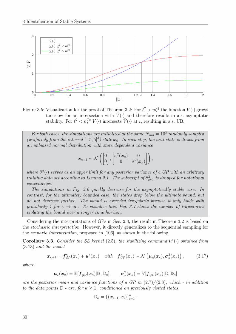
3 Identification of Stable Systems
0 0.2 0.4 0.6 0.8 1 1.2 1.4 1.6 1.8 20
1
2
3
ι‖x‖
V,V
V (·)V (·), `2 < nζ2
V (·), `2 > nζ2
Figure 3.5: Visualization for the proof of Theorem 3.2: For `2 > nζ2 the function V (·) growstoo slow for an intersection with V (·) and therefore results in a.s. asymptoticstability. For `2 < nζ2 V (·) intersects V (·) at ι, resulting in a.s. UB.
For both cases, the simulations are initialized at the same Ninit = 103 randomly sampled(uniformly from the interval [−5; 5]2) state x0. In each step, the next state is drawn froman unbiased normal distribution with state dependent variance
xκ+1 ∼ N([
00
],[σ2(xκ) 0
0 σ2(xκ)
]),
where σ2(·) serves as an upper limit for any posterior variance of a GP with an arbitrarytraining data set according to Lemma 2.1. The subscript of σ2
x(i) is dropped for notationalconvenience.The simulations in Fig. 3.6 quickly decrease for the asymptotically stable case. In
contrast, for the ultimately bounded case, the states drop below the ultimate bound, butdo not decrease further. The bound is exceeded irregularly because it only holds withprobability 1 for κ → ∞. To visualize this, Fig. 3.7 shows the number of trajectoriesviolating the bound over a longer time horizon.
Considering the interpretations of GPs in Sec. 2.3, the result in Theorem 3.2 is based onthe stochastic interpretation. However, it directly generalizes to the sequential sampling forthe scenario interpretation, proposed in [106], as shown in the following.Corollary 3.3. Consider the SE kernel (2.5), the stabilizing command u∗(·) obtained from(3.13) and the model
xκ+1 = fκGP(xκ) + u∗(xκ) with fκGP(xκ) ∼ N(µκ(xκ),σ2
κ(xκ))
, (3.17)
where
µκ(xκ) = E[fGP(xκ)|D,Dκ], σ2κ(xκ) = V[fGP(xκ)|D,Dκ]
are the posterior mean and variance functions of a GP in (2.7)/ (2.8), which - in additionto the data points D - are, for κ ≥ 1, conditioned on previously visited states
Dκ = (xi−1,xi)κi=1 .
30
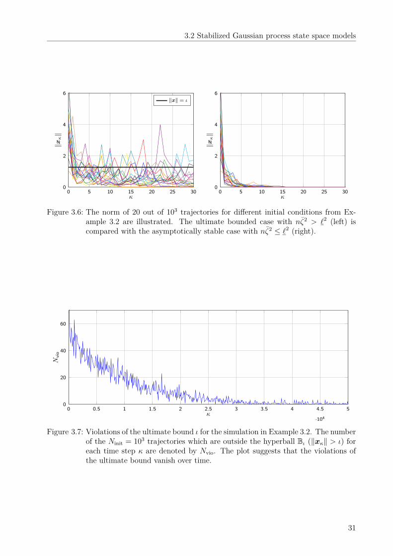
3.2 Stabilized Gaussian process state space models
0 5 10 15 20 25 300
2
4
6
κ
‖xκ‖
‖x‖ = ι
0 5 10 15 20 25 300
2
4
6
κ
‖xκ‖
Figure 3.6: The norm of 20 out of 103 trajectories for different initial conditions from Ex-ample 3.2 are illustrated. The ultimate bounded case with nζ2 > `2 (left) iscompared with the asymptotically stable case with nζ2 ≤ `2 (right).
0 0.5 1 1.5 2 2.5 3 3.5 4 4.5 5
·104
0
20
40
60
κ
Nvi
o
Figure 3.7: Violations of the ultimate bound ι for the simulation in Example 3.2. The numberof the Ninit = 103 trajectories which are outside the hyperball Bι (‖xκ‖ > ι) foreach time step κ are denoted by Nvio. The plot suggests that the violations ofthe ultimate bound vanish over time.
31
3 Identification of Stable Systems
Then, the convergence properties defined in Theorem 3.2 for (3.14) also hold for (3.17).
Proof. The system (3.17) corresponds to a sequential sampling of the function over whichthe GP describes a distribution as introduced in [106]. The convergence behavior cannotdirectly be analyzed with the previously employed Lyapunov-based methods, because thesystem is, due to the conditioning on all previously visited states, non-Markovian. However,the difference in the sequentially conditioned mean function µκ(·) and the mean function ofthe stochastic interpretation µ(·) will be accounted for by the stabilizing command u∗(·).Furthermore, based on the results in [110] it can be concluded, that σ2
κ(·) ≤ σ2(·) (element-wise, ∀x ∈ X). This ensures that the analysis based on (3.16) serves as a conservativeestimate and the convergence bounds for (3.14) also hold for (3.17).
According to Theorem 3.2, Objective 3.2 is only achieved if nζ2 < `2 holds. This constraintcould be imposed in the likelihood optimization (2.6). However, a limitation in the searchspace of the hyperparameters leads to a suboptimal model choice if the likelihood attainsits maximum outside of the constraint set. Therefore, we want to circumvent this constraintand instead propose to add additional data to the training set to achieve asymptotic stabilityfor arbitrary hyperparameters. Thus, the following section investigates how many additionalmeasurements from the system are required to satisfy Objective 3.2.
3.2.3 Convergence with additional training dataThis section considers the case nζ2 > `2, which results according to Theorem 3.2 not nec-essarily in asymptotic stability, and does not fulfill Objective 3.2. We therefore make anassumption on the availability of additional training data Dadd and elaborate how manyadditional points Nadd = |Dadd| are required to fulfill Objective 3.2.
Assumption 3.6. An additional dataset
Dadd =(x(i),y(i)
)N+Nadd
i=N+1,
can be chosen, where y(i) = f(x(i)
)is available for arbitrary input locations x(i) ∈ Bι. The
hyperparameters ψj, for all j = 1, . . . ,n of the GPSSM remain unchanged.
The assumption implies that N Nadd since otherwise the optimal hyperparameterswould significantly be affected by the updated data set. Taking data points at arbitrarylocations is a rather strict assumption, but inevitable here. We leave it to future work torelax this assumption.Without loss of generality, only a single equilibrium at the origin x∗ = 0 with domain of
attraction Rn is considered from now on. The number of required additional datapoints is de-rived as follows, where W91 : [9 exp(91); 0)→ [9∞; 91) is the lower branch of the Lambert Wfunction.
Theorem 3.3. Consider a GP (2.7)/ (2.8) with SE kernel (2.5). Then, there exists a set Daddof size
Nadd = (1 + 2ι/rtr)n + 1,
32
3.2 Stabilized Gaussian process state space models
where rtr := −`2 log(1− r2
a/nζ2)and
ra := l
3√nζ2
√√√√−nζ2W−1
(exp
(`2
nζ2 − 1)(
`2
nζ2−1))
+ `2 − nζ2
such that for any (fixed) hyperparameter set ψj, j = 1, . . . ,n the system (3.14) is a.s.asymptotically stable.
Proof. Similar to the proof of Theorem 3.2, consider
δVsq(xκ) =n∑j=1
σ2j (xκ)− xᵀ
κxκ ≤ nmaxjσ2j (xκ)− xᵀ
κxκ,
which is negative for ‖xκ‖ > ι. In a first step, we analyze the area around the origin andhow to ensure δVsq(xκ) < 0 using a single additional data point.Since the SE kernel is stationary, we can introduce the notation k(x,x′) = k(x − x′).
Furthermore, we denote the posterior variance function of a GP with hyperparameters ζ2, `2
and the dataset D2 =
(0, 0) ,(x(a),y(a)
)by σ2
D2(·). It serves as an upper bound for thevariance function maxj σ2
j (·) with dataset D2 ∪ D, for the same reasons as in Lemma 2.1.First, we analyze the single dimensional case n = 1 to obtain a location for a single
additional data point x(a) = ra which ensures nσ2D2(x) < x2 for x ∈ [0;x(a)]. According
to [137], σ2D2(·) is given by
σ2D2(x) = ζ2 − ζ2 (k(x)2 + k(ra−x)2)− 2k(ra)k(x)k(ra−x)
(ζ2)2 − k(ra)2 ,
where k(0) = ζ2 is used. Multiplying (ζ2)2 − k(ra)2 on both sides of σ2D2(x) < x2 yields the
functions
Z(ra,x) := (ζ2)3 − ζ2k(ra)2 − ζ2k(x)2 − ζ2k(ra − x)2 − 2k(ra)k(x)k(ra − x),Z(ra,x) := ((ζ2)2 − k(ra)2)x2,
for the left and right side, respectively. Their derivatives with respect to x are
∂Z(ra,x)∂x
= 2`2
(ζ2xk(x)2 − ζ2(ra − x)k(ra − x)2 + k(ra)k(x)k(ra − x)(2x− ra)
)= 2`2
(ra(k(ra)k(x)k(ra − x)− ζ2k(ra − x)2
)+ x
(ζ2k(x)2 + ζ2k(ra − x)2 − 2k(ra)k(x)k(ra−x)
) ),
∂Z(ra,x)∂x
= 2x((ζ2)2 − k(ra)2
).
Both derivatives are zero for x = 0. Thus, we consider the second derivatives evaluated atthe origin
Z ′(ra) := ∂2Z(ra, 0)∂x2 = 2
`2
((ζ2)3 − ζ2k(ra)2
(1 + r2
a
`2
)),
Z ′(ra) := ∂2Z(ra, 0)∂x2 = 2((ζ2)2 − k(ra)2).
33
3 Identification of Stable Systems
With the lower branch of the Lambert W function W−1(·), it can be shown using [138] that
nZ ′(ra)− Z ′(ra) = 2`2
(n(ζ2)3 − (ζ2)2`2 − k(ra)2
(nζ2
(1 + r2
a
`2
)− `2
))
has only one positive zero at
ra = l√nζ2
√√√√−nζ2W−1
(exp
(`2
nζ2 − 1)(
`2
nζ2 − 1))
+ `2 − nζ2.
Thus, for any x(a) ∈ [0; ra], it is concluded that nZ(ra,x)−Z(ra,x) < 0 for all x ∈(0;x(a)
].
Therefore, δVsq(x) < 0 holds ∀x ∈ (0;x(a)] if x(a) < r.In the multiple dimensional case, it can be concluded from
∥∥∥x(a)∥∥∥ < ra that δVsq(x) < 0
for all x = ax(a) with 0 < a ≤ 1. It therefore only holds on a line as visualized in Fig. 3.8on the left.To extend the result to a hyperball around the origin, we analyze the variance σ2
D2(x)as x is moved on a hypersphere centered at the origin. Defining the constants c1 = k(‖x‖)and c2 = k
(∥∥∥x(a)∥∥∥) and the variable τ =
∥∥∥x− x(a)∥∥∥, the derivative of σ2
D2(τ) with respectto τ is given by
∂σ2D2(τ)∂τ
= ∂k(τ)∂τ
−ζ2
(ζ2)2 − c22(2k(τ)− 2c1c2),
which is non-negative because ∂k(τ)∂τ≤ 0 for the SE kernel, ζ2 ≥ c2 and k(τ) ≥ c1c2 since
∥∥∥x− x(a)∥∥∥2 ≤ ‖x‖2 +
∥∥∥x(a)∥∥∥2 ⇒ exp
(−τ 2
2`2
)≥ exp
(−‖x‖2
2`2
)exp
−∥∥∥x(a)
∥∥∥2
2`2
according to the triangle inequality. We conclude that the point with the highest varianceon the hypersphere lies on the opposite side of the point x(a)
σ2D2
(−x(a)
)= max‖x‖=‖x(a)‖
σ2D2(x),
as illustrated in Fig. 3.8 (center).As a result, x(a) must be chosen close enough to the origin, such that there exists a ra for
which all points ‖x‖ < ra are closer to x(a), than to x(a),∥∥∥x(a)+ x∥∥∥ ≤ ∥∥∥x(a)
∥∥∥+ ‖x‖ ≤∥∥∥x(a)− x
∥∥∥ =∥∥∥x(a)
∥∥∥− ‖x‖∥∥∥x(a)∥∥∥+ 2‖x‖ ≤
∥∥∥x(a)∥∥∥ ⇒
∥∥∥x(a)∥∥∥ ≤ 1
3∥∥∥x(a)
∥∥∥,which yields ra := ra/3.So for the multidimensional case, it holds for all x with 0 < ‖x‖ < ra that nσ2
D2(x) < ‖x‖2
if∥∥∥x(a)
∥∥∥ ≤ ra. Thus we set x(N+1) = x(a) according to Assumption 3.6.
34
3.3 Learning Lyapunov functions for stabilization
If ra > ι, the proof is completed since then nσ2D2(x) < ‖x‖2 holds for all x ∈ X with one
additional training point.For, ra ≤ ι, the region ra ≤ ‖x‖ ≤ ι, must be covered with enough training data to
ensure nσ2D2(x) < ‖x‖2 everywhere. For simplicity, we show that nσ2
D2(x) < r2a is ensured
for all ‖x‖ < ι. From the bound in Lemma 2.1, it follows that every additional datapoint x(i), i ∈ N + 2, . . . , N + Nadd upper bounds the variance function in a radius rtrgiven by
∥∥∥x− x(i)∥∥∥2< rtr ⇒ σ2
j (x) ≤ nζ2(
1− exp(−‖x− x(i)‖2
`2
))≤ r2
a.
The number of hyperballs with radius rtr required to cover a (larger) hyperball with radius ιis given by the covering number. In [139] the upper bound on the covering number is givenby (1+2ι/rtr)n. Therefore, not more than (1+2ι/rtr)n+1 additional data points are requiredto ensure δVsq(xκ) < 0 ∀x \ 0, which concludes the proof.
Example 3.3. Reconsider Example 3.2 with n = 2, `2 = 1 and ζ2 = 1, for which ι ≈ 1.26was obtained. According to Theorem 3.3, one training point x(a) must be chosen nearthe origin with ra ≈ 0.37 (ra ≈ 1.12). Figure 3.9 compares different choices of the firstadditional data point x(a). With rtr ≈ 0.0724 a maximum of Nadd = 1290 additionaltraining points is required to ensure a.s. asymptotic stability.
3.3 Learning Lyapunov functions for stabilizationFor the stabilization of a GPSSM as presented in Sec. 3.2, any control Lyapunov function(subject to Assumptions 3.4 and 3.5) is applicable. However, the GPSSM fGP(·) withoutstabilization is the best fit to the data and therefore should only be minimally distortedby the stabilization u(·). This requires an optimal choice of the Lyapunov functions V i∗
θi∗(·)
based on the available data to properly describe the convergence behavior of the model.This section presents a general framework for a data-driven optimization-based estimationof the convergence behavior including the equilibria and discusses three specific choices forthe Lyapunov candidates.
3.3.1 Optimization-based formulationConsider Lyapunov functions V i∗
θi∗(·) which are parameterized by θi∗ ∈ Θi∗ and the estimated
equilibrium xi∗ ∈ Xi∗ . For fitting these parameters to the training set D, the following isconcluded.
Proposition 3.4. Consider N∗ Lyapunov candidates V i∗θi∗
(·) under Assumptions 3.4 and 3.5and the dataset from Assumption 3.2. Furthermore, consider Ii∗ =
i = 1, . . . ,N
∣∣∣x(i) ∈ Xi∗
and g : R→ R+, which is any function of the form
g(ξ) =0 for ξ ≤ 0g(ξ) for ξ > 0
with g(ξ) > 0 ∀ξ. (3.18)
35
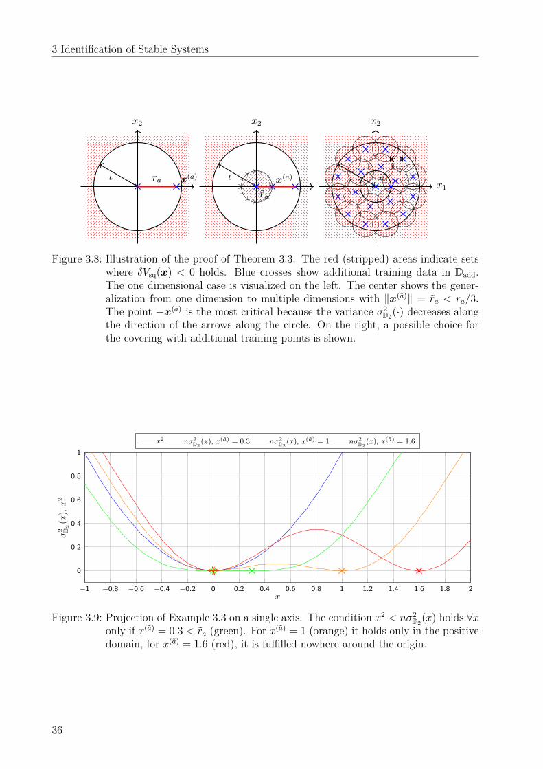
3 Identification of Stable Systems
ι
x2
ra x(a) ι
x2
x(a)
ra
rtr
x2
x1ra
Figure 3.8: Illustration of the proof of Theorem 3.3. The red (stripped) areas indicate setswhere δVsq(x) < 0 holds. Blue crosses show additional training data in Dadd.The one dimensional case is visualized on the left. The center shows the gener-alization from one dimension to multiple dimensions with ‖x(a)‖ = ra < ra/3.The point −x(a) is the most critical because the variance σ2
D2(·) decreases alongthe direction of the arrows along the circle. On the right, a possible choice forthe covering with additional training points is shown.
−1 −0.8 −0.6 −0.4 −0.2 0 0.2 0.4 0.6 0.8 1 1.2 1.4 1.6 1.8 2
0
0.2
0.4
0.6
0.8
1
x
σ2 D 2
(x),x
2
x2 nσ2D2
(x), x(a) = 0.3 nσ2D2
(x), x(a) = 1 nσ2D2
(x), x(a) = 1.6
Figure 3.9: Projection of Example 3.3 on a single axis. The condition x2 < nσ2D2(x) holds ∀x
only if x(a) = 0.3 < ra (green). For x(a) = 1 (orange) it holds only in the positivedomain, for x(a) = 1.6 (red), it is fulfilled nowhere around the origin.
36
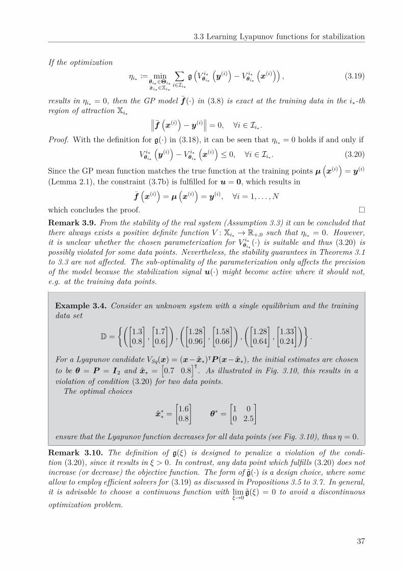
3.3 Learning Lyapunov functions for stabilization
If the optimizationηi∗ := min
θi∗∈Θi∗xi∗∈Xi∗
∑i∈Ii∗
g(V i∗θi∗
(y(i)
)− V i∗
θi∗
(x(i)
)), (3.19)
results in ηi∗ = 0, then the GP model f(·) in (3.8) is exact at the training data in the i∗-thregion of attraction Xi∗ ∥∥∥f (x(i)
)− y(i)
∥∥∥ = 0, ∀i ∈ Ii∗ .Proof. With the definition for g(·) in (3.18), it can be seen that ηi∗ = 0 holds if and only if
V i∗θi∗
(y(i)
)− V i∗
θi∗
(x(i)
)≤ 0, ∀i ∈ Ii∗ . (3.20)
Since the GP mean function matches the true function at the training points µ(x(i)
)= y(i)
(Lemma 2.1), the constraint (3.7b) is fulfilled for u = 0, which results in
f(x(i)
)= µ
(x(i)
)= y(i), ∀i = 1, . . . ,N
which concludes the proof.Remark 3.9. From the stability of the real system (Assumption 3.3) it can be concluded thatthere always exists a positive definite function V : Xi∗ → R+,0 such that ηi∗ = 0. However,it is unclear whether the chosen parameterization for V i∗
θi∗(·) is suitable and thus (3.20) is
possibly violated for some data points. Nevertheless, the stability guarantees in Theorems 3.1to 3.3 are not affected. The sub-optimality of the parameterization only affects the precisionof the model because the stabilization signal u(·) might become active where it should not,e.g. at the training data points.
Example 3.4. Consider an unknown system with a single equilibrium and the trainingdata set
D =([
1.30.8
],[1.70.6
]),([
1.280.96
],[1.580.66
]),([
1.280.64
],[1.330.24
]).
For a Lyapunov candidate VSq(x) = (x− x∗)ᵀP (x− x∗), the initial estimates are chosento be θ = P = I2 and x∗ =
[0.7 0.8
]ᵀ. As illustrated in Fig. 3.10, this results in a
violation of condition (3.20) for two data points.The optimal choices
x∗∗ =[1.60.8
]θ∗ =
[1 00 2.5
]
ensure that the Lyapunov function decreases for all data points (see Fig. 3.10), thus η = 0.
Remark 3.10. The definition of g(ξ) is designed to penalize a violation of the condi-tion (3.20), since it results in ξ > 0. In contrast, any data point which fulfills (3.20) does notincrease (or decrease) the objective function. The form of g(·) is a design choice, where someallow to employ efficient solvers for (3.19) as discussed in Propositions 3.5 to 3.7. In general,it is advisable to choose a continuous function with lim
ξ→0g(ξ) = 0 to avoid a discontinuous
optimization problem.
37
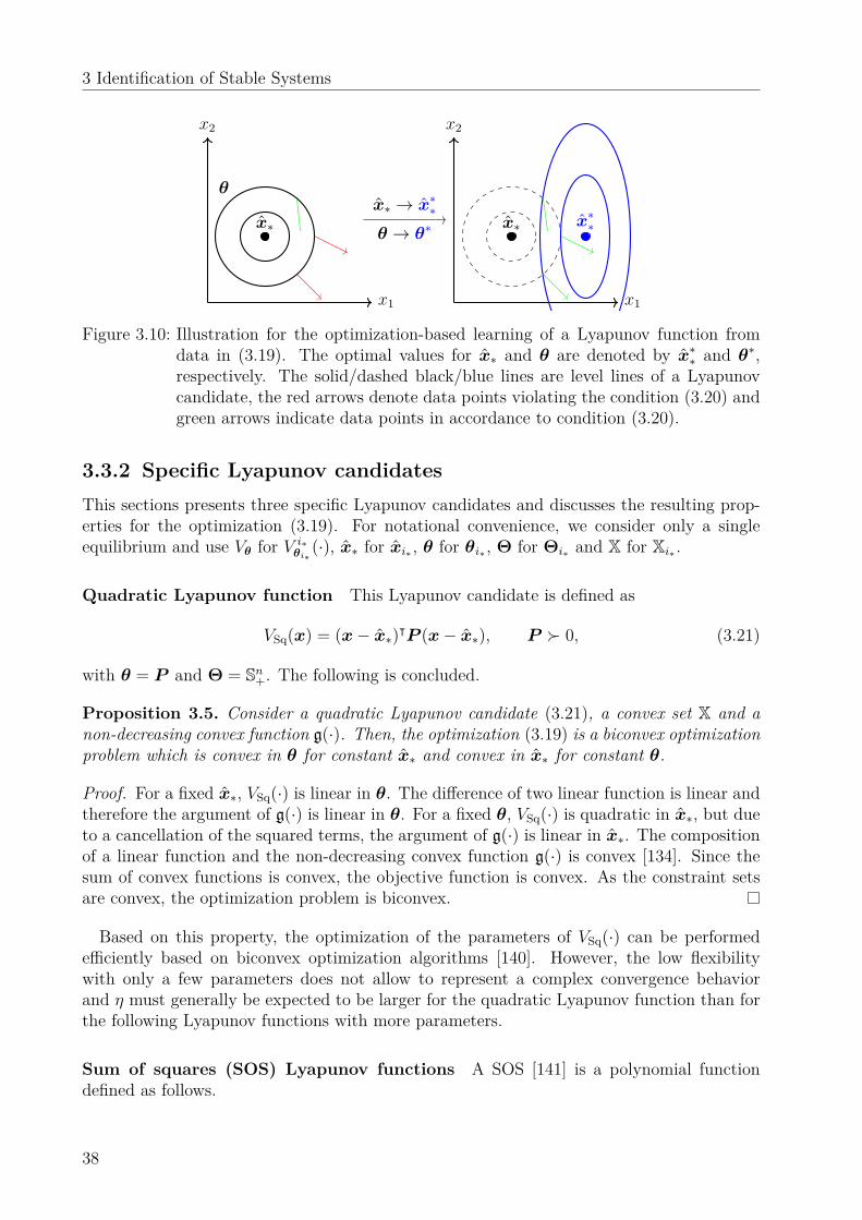
3 Identification of Stable Systems
x1
x2
x∗
θx∗ → x∗
∗
θ → θ∗
x1
x2
x∗ x∗∗
Figure 3.10: Illustration for the optimization-based learning of a Lyapunov function fromdata in (3.19). The optimal values for x∗ and θ are denoted by x∗∗ and θ∗,respectively. The solid/dashed black/blue lines are level lines of a Lyapunovcandidate, the red arrows denote data points violating the condition (3.20) andgreen arrows indicate data points in accordance to condition (3.20).
3.3.2 Specific Lyapunov candidatesThis sections presents three specific Lyapunov candidates and discusses the resulting prop-erties for the optimization (3.19). For notational convenience, we consider only a singleequilibrium and use Vθ for V i∗
θi∗(·), x∗ for xi∗ , θ for θi∗ , Θ for Θi∗ and X for Xi∗ .
Quadratic Lyapunov function This Lyapunov candidate is defined as
VSq(x) = (x− x∗)ᵀP (x− x∗), P 0, (3.21)
with θ = P and Θ = Sn+. The following is concluded.
Proposition 3.5. Consider a quadratic Lyapunov candidate (3.21), a convex set X and anon-decreasing convex function g(·). Then, the optimization (3.19) is a biconvex optimizationproblem which is convex in θ for constant x∗ and convex in x∗ for constant θ.
Proof. For a fixed x∗, VSq(·) is linear in θ. The difference of two linear function is linear andtherefore the argument of g(·) is linear in θ. For a fixed θ, VSq(·) is quadratic in x∗, but dueto a cancellation of the squared terms, the argument of g(·) is linear in x∗. The compositionof a linear function and the non-decreasing convex function g(·) is convex [134]. Since thesum of convex functions is convex, the objective function is convex. As the constraint setsare convex, the optimization problem is biconvex.
Based on this property, the optimization of the parameters of VSq(·) can be performedefficiently based on biconvex optimization algorithms [140]. However, the low flexibilitywith only a few parameters does not allow to represent a complex convergence behaviorand η must generally be expected to be larger for the quadratic Lyapunov function than forthe following Lyapunov functions with more parameters.
Sum of squares (SOS) Lyapunov functions A SOS [141] is a polynomial functiondefined as follows.
38
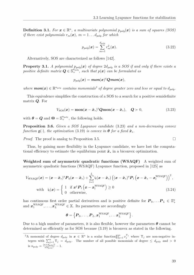
3.3 Learning Lyapunov functions for stabilization
Definition 3.1. For x ∈ Rn, a multivariate polynomial ppoly(x) is a sum of squares (SOS)if there exist polynomials rm(x), m = 1 . . . dpoly for which
ppoly(x) =dpoly∑m=1
r2m(x). (3.22)
Alternatively, SOS are characterized as follows [142].
Property 3.1. A polynomial ppoly(x) of degree 2dpoly is a SOS if and only if there exists apositive definite matrix Q ∈ Snpoly
+ , such that p(x) can be formulated as
ppoly(x) = mon(x)ᵀQmon(x),
where mon(x) ∈ Rnpoly contains monomials3 of degree greater zero and less or equal to dpoly.
This equivalence simplifies the construction of a SOS to a search for a positive semidefinitematrix Q. For
VSOS(x) = mon(x− x∗)ᵀQmon(x− x∗), Q 0, (3.23)
with θ = Q and Θ = Snpoly+ , the following holds.
Proposition 3.6. Given a SOS Lyapunov candidate (3.23) and a non-decreasing convexfunction g(·), the optimization (3.19) is convex in θ for a fixed x∗.
Proof. The proof is analog to Proposition 3.5.
Thus, by gaining more flexibility in the Lyapunov candidate, we have lost the computa-tional efficiency to estimate the equilibrium point x∗ in a biconvex optimization.
Weighted sum of asymmetric quadratic functions (WSAQF) A weighted sum ofasymmetric quadratic functions (WSAQF) Lyapunov function, proposed in [125] as
VWSAQF(x) = (x− x∗)ᵀP 0(x− x∗) +L∑l=1
il(x− x∗)((x− x∗)ᵀP l
(x− x∗ − xWSAQF
l
))2,
with il(x) =
1 if xᵀP l
(x− xWSAQF
l
)≥ 0
0 otherwise,(3.24)
has continuous first order partial derivatives and is positive definite for P 0, . . .P L ∈ Sn+and xWSAQF
1 , . . . ,xWSAQFL ∈ X. Its parameters are accordingly
θ =P 0, . . . ,P L,xWSAQF
1 , . . .xWSAQFL
.
Due to a high number of parameters, it is also flexible, however the parameters θ cannot bedetermined as efficiently as for SOS because (3.19) is biconvex as stated in the following.
3A monomial of degree dpoly in x ∈ Rn is a scalar function∏nj=1 x
Υj
j where Υj are non-negative in-tegers with
∑nj=1 Υj = dpoly. The number of all possible monomials of degree ≤ dpoly and > 0
is npoly = (n+dpoly)!n!dpoly! − 1.
39
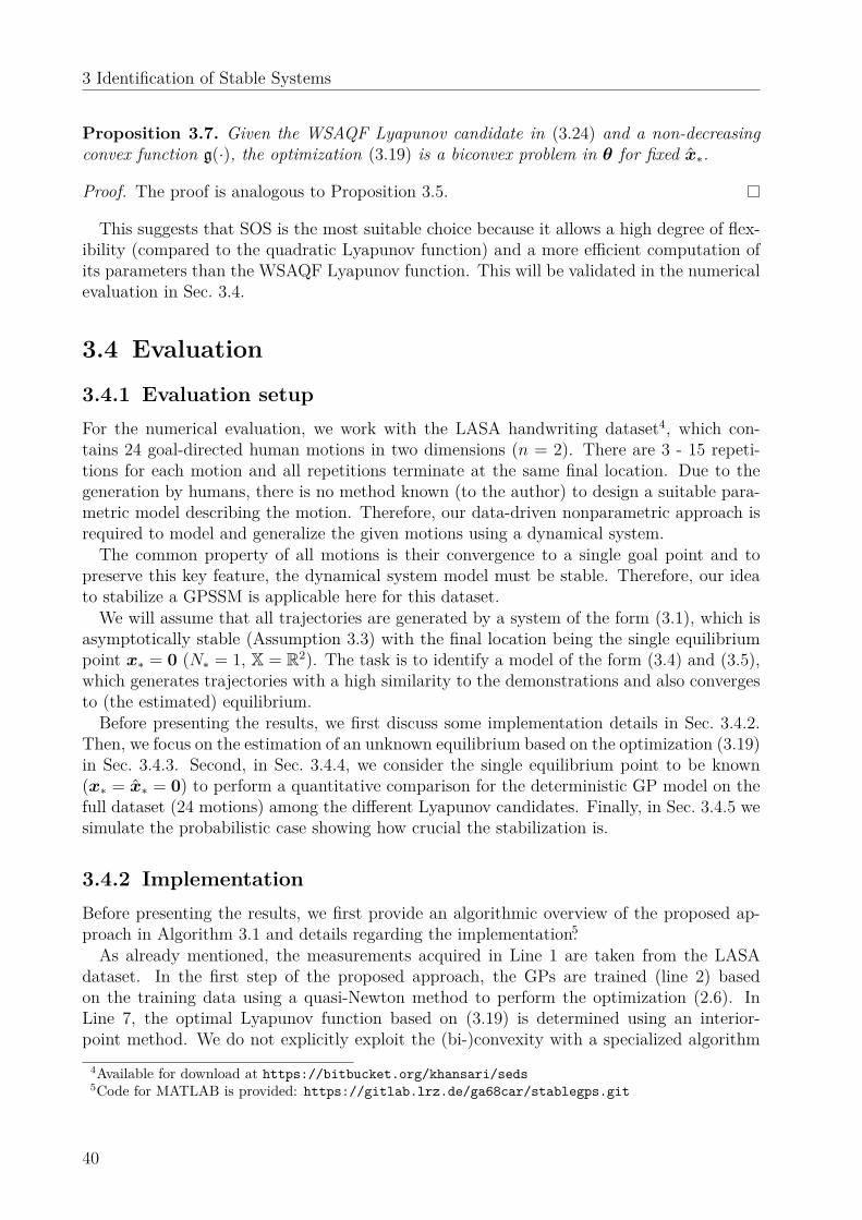
3 Identification of Stable Systems
Proposition 3.7. Given the WSAQF Lyapunov candidate in (3.24) and a non-decreasingconvex function g(·), the optimization (3.19) is a biconvex problem in θ for fixed x∗.
Proof. The proof is analogous to Proposition 3.5.
This suggests that SOS is the most suitable choice because it allows a high degree of flex-ibility (compared to the quadratic Lyapunov function) and a more efficient computation ofits parameters than the WSAQF Lyapunov function. This will be validated in the numericalevaluation in Sec. 3.4.
3.4 Evaluation
3.4.1 Evaluation setupFor the numerical evaluation, we work with the LASA handwriting dataset4, which con-tains 24 goal-directed human motions in two dimensions (n = 2). There are 3 - 15 repeti-tions for each motion and all repetitions terminate at the same final location. Due to thegeneration by humans, there is no method known (to the author) to design a suitable para-metric model describing the motion. Therefore, our data-driven nonparametric approach isrequired to model and generalize the given motions using a dynamical system.The common property of all motions is their convergence to a single goal point and to
preserve this key feature, the dynamical system model must be stable. Therefore, our ideato stabilize a GPSSM is applicable here for this dataset.We will assume that all trajectories are generated by a system of the form (3.1), which is
asymptotically stable (Assumption 3.3) with the final location being the single equilibriumpoint x∗ = 0 (N∗ = 1, X = R2). The task is to identify a model of the form (3.4) and (3.5),which generates trajectories with a high similarity to the demonstrations and also convergesto (the estimated) equilibrium.Before presenting the results, we first discuss some implementation details in Sec. 3.4.2.
Then, we focus on the estimation of an unknown equilibrium based on the optimization (3.19)in Sec. 3.4.3. Second, in Sec. 3.4.4, we consider the single equilibrium point to be known(x∗ = x∗ = 0) to perform a quantitative comparison for the deterministic GP model on thefull dataset (24 motions) among the different Lyapunov candidates. Finally, in Sec. 3.4.5 wesimulate the probabilistic case showing how crucial the stabilization is.
3.4.2 ImplementationBefore presenting the results, we first provide an algorithmic overview of the proposed ap-proach in Algorithm 3.1 and details regarding the implementation.5As already mentioned, the measurements acquired in Line 1 are taken from the LASA
dataset. In the first step of the proposed approach, the GPs are trained (line 2) basedon the training data using a quasi-Newton method to perform the optimization (2.6). InLine 7, the optimal Lyapunov function based on (3.19) is determined using an interior-point method. We do not explicitly exploit the (bi-)convexity with a specialized algorithm
4Available for download at https://bitbucket.org/khansari/seds5Code for MATLAB is provided: https://gitlab.lrz.de/ga68car/stablegps.git
40
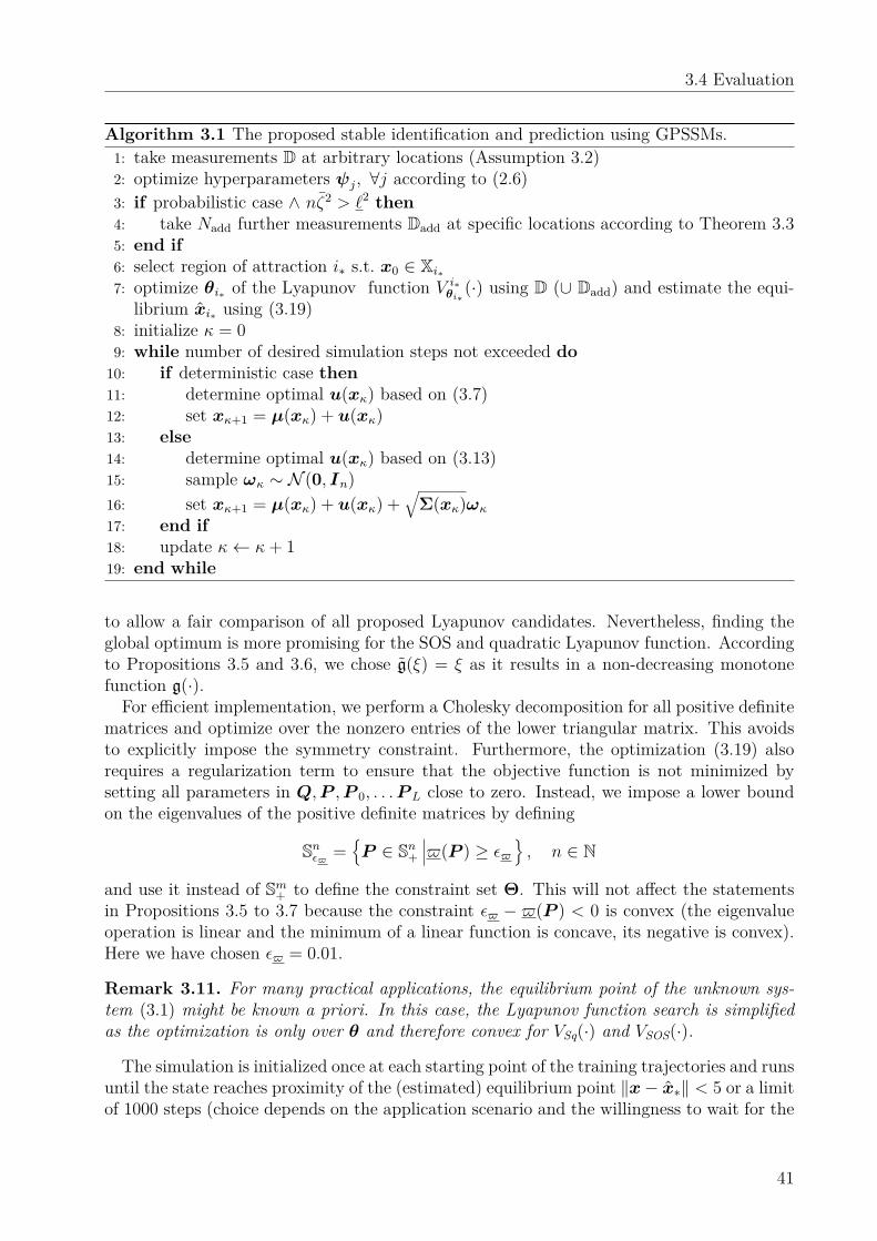
3.4 Evaluation
Algorithm 3.1 The proposed stable identification and prediction using GPSSMs.1: take measurements D at arbitrary locations (Assumption 3.2)2: optimize hyperparameters ψj, ∀j according to (2.6)3: if probabilistic case ∧ nζ2 > `2 then4: take Nadd further measurements Dadd at specific locations according to Theorem 3.35: end if6: select region of attraction i∗ s.t. x0 ∈ Xi∗7: optimize θi∗ of the Lyapunov function V i∗
θi∗(·) using D (∪ Dadd) and estimate the equi-
librium xi∗ using (3.19)8: initialize κ = 09: while number of desired simulation steps not exceeded do10: if deterministic case then11: determine optimal u(xκ) based on (3.7)12: set xκ+1 = µ(xκ) + u(xκ)13: else14: determine optimal u(xκ) based on (3.13)15: sample ωκ ∼ N (0, In)16: set xκ+1 = µ(xκ) + u(xκ) +
√Σ(xκ)ωκ
17: end if18: update κ← κ+ 119: end while
to allow a fair comparison of all proposed Lyapunov candidates. Nevertheless, finding theglobal optimum is more promising for the SOS and quadratic Lyapunov function. Accordingto Propositions 3.5 and 3.6, we chose g(ξ) = ξ as it results in a non-decreasing monotonefunction g(·).For efficient implementation, we perform a Cholesky decomposition for all positive definite
matrices and optimize over the nonzero entries of the lower triangular matrix. This avoidsto explicitly impose the symmetry constraint. Furthermore, the optimization (3.19) alsorequires a regularization term to ensure that the objective function is not minimized bysetting all parameters in Q,P ,P 0, . . .P L close to zero. Instead, we impose a lower boundon the eigenvalues of the positive definite matrices by defining
Snε$ =P ∈ Sn+
∣∣∣$(P ) ≥ ε$
, n ∈ N
and use it instead of Sm+ to define the constraint set Θ. This will not affect the statementsin Propositions 3.5 to 3.7 because the constraint ε$ − $(P ) < 0 is convex (the eigenvalueoperation is linear and the minimum of a linear function is concave, its negative is convex).Here we have chosen ε$ = 0.01.
Remark 3.11. For many practical applications, the equilibrium point of the unknown sys-tem (3.1) might be known a priori. In this case, the Lyapunov function search is simplifiedas the optimization is only over θ and therefore convex for VSq(·) and VSOS(·).
The simulation is initialized once at each starting point of the training trajectories and runsuntil the state reaches proximity of the (estimated) equilibrium point ‖x− x∗‖ < 5 or a limitof 1000 steps (choice depends on the application scenario and the willingness to wait for the
41
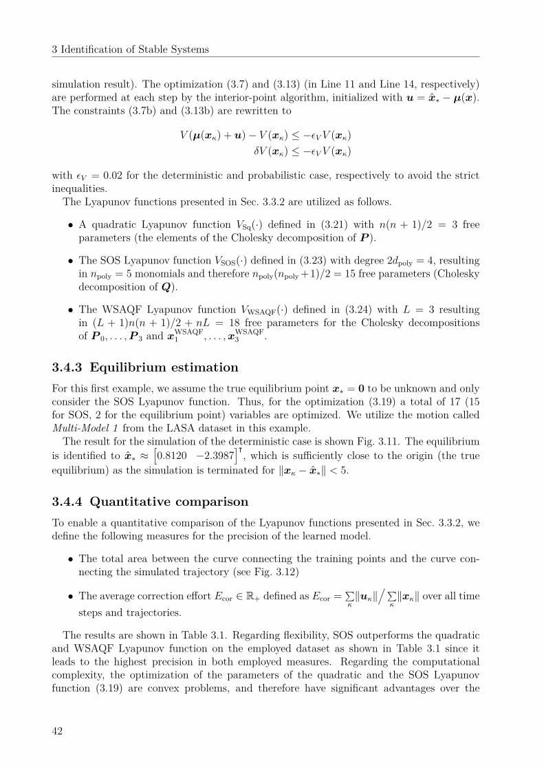
3 Identification of Stable Systems
simulation result). The optimization (3.7) and (3.13) (in Line 11 and Line 14, respectively)are performed at each step by the interior-point algorithm, initialized with u = x∗ − µ(x).The constraints (3.7b) and (3.13b) are rewritten to
V (µ(xκ) + u)− V (xκ) ≤ −εV V (xκ)δV (xκ) ≤ −εV V (xκ)
with εV = 0.02 for the deterministic and probabilistic case, respectively to avoid the strictinequalities.The Lyapunov functions presented in Sec. 3.3.2 are utilized as follows.
• A quadratic Lyapunov function VSq(·) defined in (3.21) with n(n + 1)/2 = 3 freeparameters (the elements of the Cholesky decomposition of P ).
• The SOS Lyapunov function VSOS(·) defined in (3.23) with degree 2dpoly = 4, resultingin npoly = 5 monomials and therefore npoly(npoly +1)/2 = 15 free parameters (Choleskydecomposition of Q).
• The WSAQF Lyapunov function VWSAQF(·) defined in (3.24) with L = 3 resultingin (L + 1)n(n + 1)/2 + nL = 18 free parameters for the Cholesky decompositionsof P 0, . . . ,P 3 and xWSAQF
1 , . . . ,xWSAQF3 .
3.4.3 Equilibrium estimationFor this first example, we assume the true equilibrium point x∗ = 0 to be unknown and onlyconsider the SOS Lyapunov function. Thus, for the optimization (3.19) a total of 17 (15for SOS, 2 for the equilibrium point) variables are optimized. We utilize the motion calledMulti-Model 1 from the LASA dataset in this example.The result for the simulation of the deterministic case is shown Fig. 3.11. The equilibrium
is identified to x∗ ≈[0.8120 −2.3987
]ᵀ, which is sufficiently close to the origin (the true
equilibrium) as the simulation is terminated for ‖xκ − x∗‖ < 5.
3.4.4 Quantitative comparisonTo enable a quantitative comparison of the Lyapunov functions presented in Sec. 3.3.2, wedefine the following measures for the precision of the learned model.
• The total area between the curve connecting the training points and the curve con-necting the simulated trajectory (see Fig. 3.12)
• The average correction effort Ecor ∈ R+ defined as Ecor = ∑κ‖uκ‖
/∑κ‖xκ‖ over all time
steps and trajectories.
The results are shown in Table 3.1. Regarding flexibility, SOS outperforms the quadraticand WSAQF Lyapunov function on the employed dataset as shown in Table 3.1 since itleads to the highest precision in both employed measures. Regarding the computationalcomplexity, the optimization of the parameters of the quadratic and the SOS Lyapunovfunction (3.19) are convex problems, and therefore have significant advantages over the
42
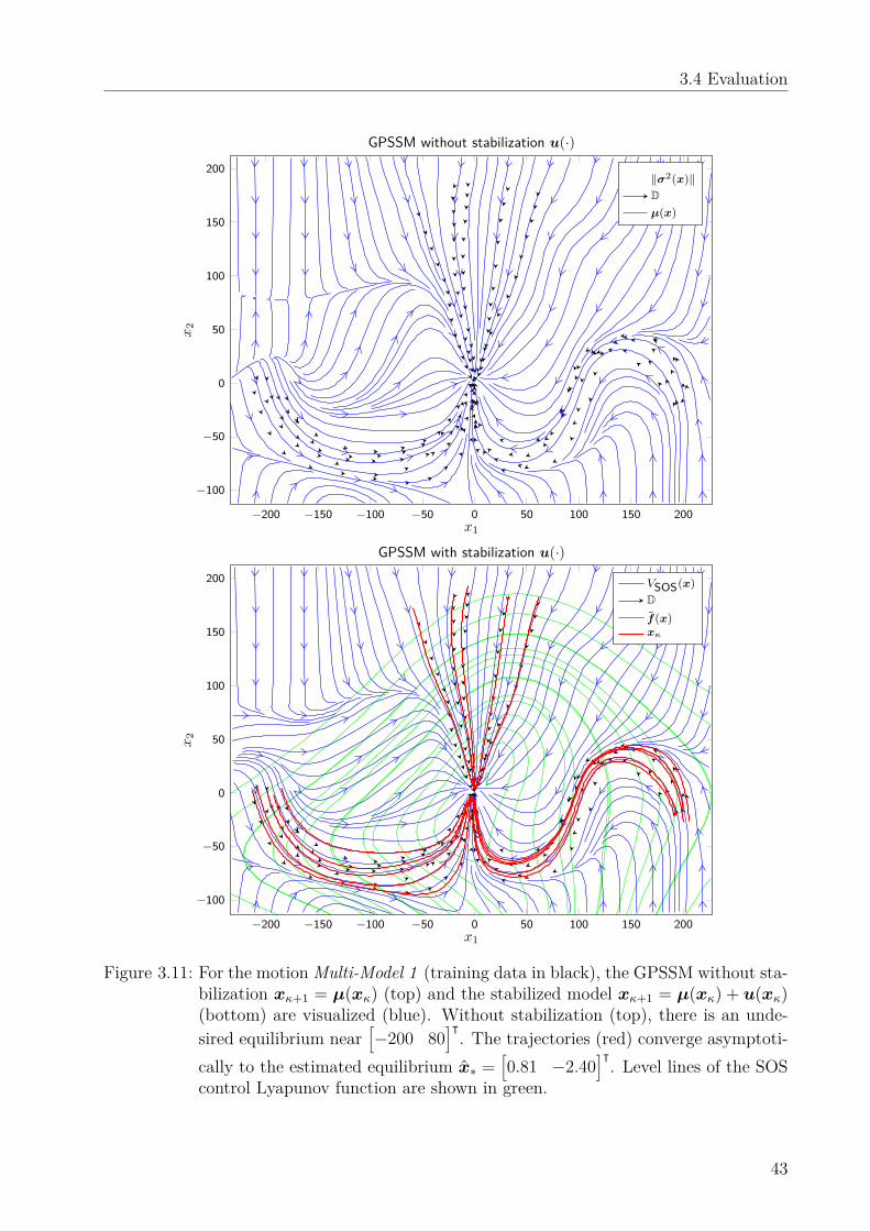
3.4 Evaluation
−200 −150 −100 −50 0 50 100 150 200
−100
−50
0
50
100
150
200
x1
x2
GPSSM without stabilization u(·)
‖σ2(x)‖Dµ(x)
−200 −150 −100 −50 0 50 100 150 200
−100
−50
0
50
100
150
200
x1
x2
GPSSM with stabilization u(·)
VSOS(x)Df(x)xκ
Figure 3.11: For the motion Multi-Model 1 (training data in black), the GPSSM without sta-bilization xκ+1 = µ(xκ) (top) and the stabilized model xκ+1 = µ(xκ) + u(xκ)(bottom) are visualized (blue). Without stabilization (top), there is an unde-sired equilibrium near
[−200 80
]ᵀ. The trajectories (red) converge asymptoti-
cally to the estimated equilibrium x∗ =[0.81 −2.40
]ᵀ. Level lines of the SOS
control Lyapunov function are shown in green.
43
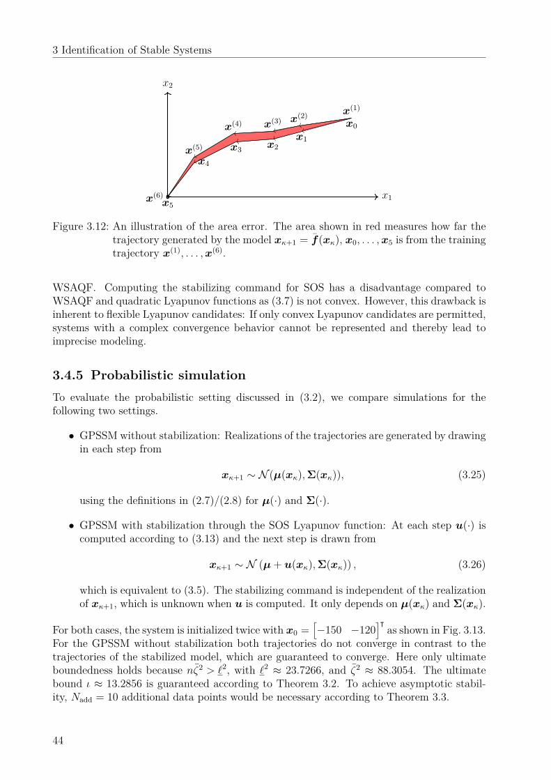
3 Identification of Stable Systems
x1
x2
x5x(6)
x(1)x(2)
x(3)x(4)
x(5)
x0x1
x2x3x4
Figure 3.12: An illustration of the area error. The area shown in red measures how far thetrajectory generated by the model xκ+1 = f(xκ), x0, . . . ,x5 is from the trainingtrajectory x(1), . . . ,x(6).
WSAQF. Computing the stabilizing command for SOS has a disadvantage compared toWSAQF and quadratic Lyapunov functions as (3.7) is not convex. However, this drawback isinherent to flexible Lyapunov candidates: If only convex Lyapunov candidates are permitted,systems with a complex convergence behavior cannot be represented and thereby lead toimprecise modeling.
3.4.5 Probabilistic simulationTo evaluate the probabilistic setting discussed in (3.2), we compare simulations for thefollowing two settings.
• GPSSM without stabilization: Realizations of the trajectories are generated by drawingin each step from
xκ+1 ∼ N (µ(xκ), Σ(xκ)), (3.25)
using the definitions in (2.7)/(2.8) for µ(·) and Σ(·).
• GPSSM with stabilization through the SOS Lyapunov function: At each step u(·) iscomputed according to (3.13) and the next step is drawn from
xκ+1 ∼ N (µ+ u(xκ), Σ(xκ)) , (3.26)
which is equivalent to (3.5). The stabilizing command is independent of the realizationof xκ+1, which is unknown when u is computed. It only depends on µ(xκ) and Σ(xκ).
For both cases, the system is initialized twice with x0 =[−150 −120
]ᵀas shown in Fig. 3.13.
For the GPSSM without stabilization both trajectories do not converge in contrast to thetrajectories of the stabilized model, which are guaranteed to converge. Here only ultimateboundedness holds because nζ2 > `2, with `2 ≈ 23.7266, and ζ2 ≈ 88.3054. The ultimatebound ι ≈ 13.2856 is guaranteed according to Theorem 3.2. To achieve asymptotic stabil-ity, Nadd = 10 additional data points would be necessary according to Theorem 3.3.
44
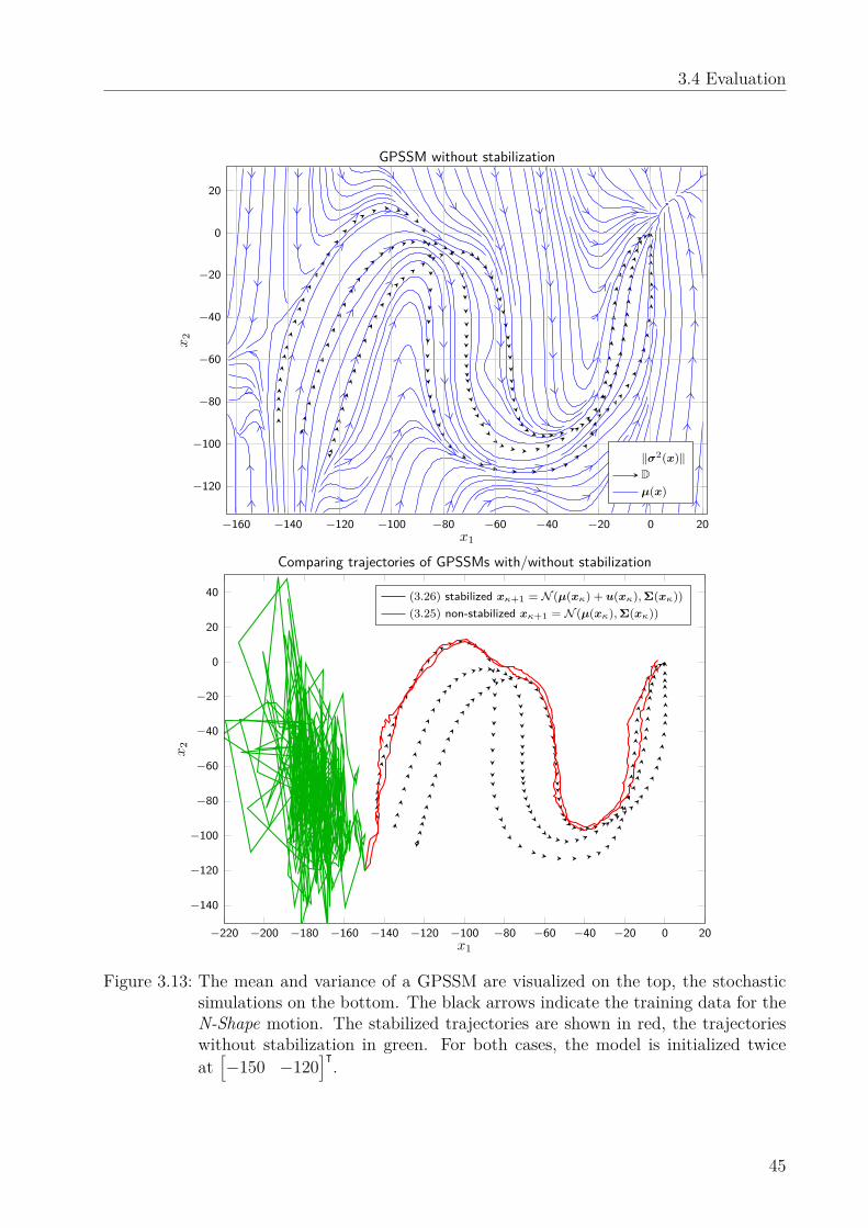
3.4 Evaluation
−160 −140 −120 −100 −80 −60 −40 −20 0 20
−120
−100
−80
−60
−40
−20
0
20
x1
x2
GPSSM without stabilization
‖σ2(x)‖Dµ(x)
−220 −200 −180 −160 −140 −120 −100 −80 −60 −40 −20 0 20
−140
−120
−100
−80
−60
−40
−20
0
20
40
x1
x2
Comparing trajectories of GPSSMs with/without stabilization
(3.26) stabilized xκ+1 = N (µ(xκ) + u(xκ), Σ(xκ))(3.25) non-stabilized xκ+1 = N (µ(xκ), Σ(xκ))
Figure 3.13: The mean and variance of a GPSSM are visualized on the top, the stochasticsimulations on the bottom. The black arrows indicate the training data for theN-Shape motion. The stabilized trajectories are shown in red, the trajectorieswithout stabilization in green. For both cases, the model is initialized twiceat[−150 −120
]ᵀ.
45
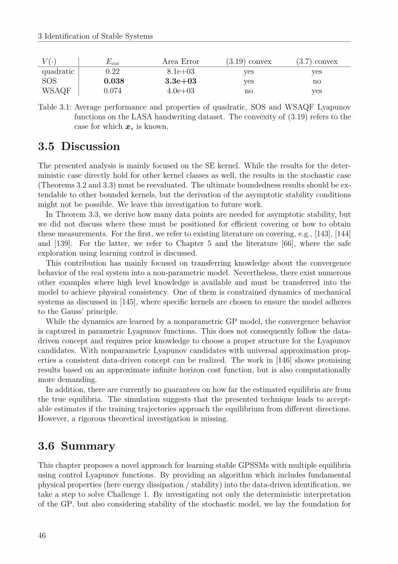
3 Identification of Stable Systems
V (·) Ecor Area Error (3.19) convex (3.7) convexquadratic 0.22 8.1e+03 yes yesSOS 0.038 3.3e+03 yes noWSAQF 0.074 4.0e+03 no yes
Table 3.1: Average performance and properties of quadratic, SOS and WSAQF Lyapunovfunctions on the LASA handwriting dataset. The convexity of (3.19) refers to thecase for which x∗ is known.
3.5 DiscussionThe presented analysis is mainly focused on the SE kernel. While the results for the deter-ministic case directly hold for other kernel classes as well, the results in the stochastic case(Theorems 3.2 and 3.3) must be reevaluated. The ultimate boundedness results should be ex-tendable to other bounded kernels, but the derivation of the asymptotic stability conditionsmight not be possible. We leave this investigation to future work.In Theorem 3.3, we derive how many data points are needed for asymptotic stability, but
we did not discuss where these must be positioned for efficient covering or how to obtainthese measurements. For the first, we refer to existing literature on covering, e.g., [143], [144]and [139]. For the latter, we refer to Chapter 5 and the literature [66], where the safeexploration using learning control is discussed.This contribution has mainly focused on transferring knowledge about the convergence
behavior of the real system into a non-parametric model. Nevertheless, there exist numerousother examples where high level knowledge is available and must be transferred into themodel to achieve physical consistency. One of them is constrained dynamics of mechanicalsystems as discussed in [145], where specific kernels are chosen to ensure the model adheresto the Gauss’ principle.While the dynamics are learned by a nonparametric GP model, the convergence behavior
is captured in parametric Lyapunov functions. This does not consequently follow the data-driven concept and requires prior knowledge to choose a proper structure for the Lyapunovcandidates. With nonparametric Lyapunov candidates with universal approximation prop-erties a consistent data-driven concept can be realized. The work in [146] shows promisingresults based on an approximate infinite horizon cost function, but is also computationallymore demanding.In addition, there are currently no guarantees on how far the estimated equilibria are from
the true equilibria. The simulation suggests that the presented technique leads to accept-able estimates if the training trajectories approach the equilibrium from different directions.However, a rigorous theoretical investigation is missing.
3.6 SummaryThis chapter proposes a novel approach for learning stable GPSSMs with multiple equilibriausing control Lyapunov functions. By providing an algorithm which includes fundamentalphysical properties (here energy dissipation / stability) into the data-driven identification, wetake a step to solve Challenge 1. By investigating not only the deterministic interpretationof the GP, but also considering stability of the stochastic model, we lay the foundation for
46

3.6 Summary
uncertainty aware control laws (Challenge 3).For the deterministic case, we show (global) asymptotic stability of the model and prove
that the stabilization will never reduce the precision of the GP model (if the Lyapunov func-tions are chosen correctly). For the stochastic case, we show (global) ultimate boundednessand derive an upper bound for the number of additional training data which are required toensure asymptotic stability independently of the kernel parameters.A generic framework to learn the convergence behavior of dynamical systems from training
data is presented in this chapter. This includes data-driven optimization-based adaptationof a parametric Lyapunov candidate and an estimation of the equilibria. Furthermore, wederive (bi-)convexity results for different types of Lyapunov candidates to ensure the requiredoptimization can be performed efficiently. The numerical analysis based on a real-worldhuman motion data set shows that SOS Lyapunov functions are well suited for data-drivenlearning of the convergence behavior of dynamical systems.
47

Uncertainty-basedControl Lyapunov Design 4
Uncertainties in a control loop can arise from various sources, e.g., measurements of theoutput can be corrupted by noise, the process itself can be of stochastic nature or themodel of the process is imprecise. Incorporating these uncertainties into the control designbecomes particularly important in safety-critical applications and various techniques havebeen developed to handle uncertainties properly.Robust control is a basic concept to ensure proper operation under a bounded model
error and allows to provide stability guarantees for closed-loop systems under specific as-sumptions [147]. However, these assumptions are often not easy to justify and lead to aconservative strategy, which sacrifices control performance [148]. Alternatively, stochasticcontrol can also handle uncertainties in the system and perform a profound stability analysisbased on the stochastic differential equations [128], [149], [150]. But this technique considersuncertainty as a random behavior, rather than ignorance of the true dynamics.Based on optimal control, various differential dynamic programming approaches are ex-
tended to deal with uncertain systems [44]. These predictive control techniques take thefuture uncertainty implicitly into account for their control decision [151]. Extensions whichallow to explicitly weight the future uncertainties in the cost function are presented in [129],[152], [153] known as risk-sensitive or uncertainty-dependent control design. However, sta-bility or safety guarantees for these methods do not exist.Since GPs provide a model fidelity measure, they are well suited for an uncertainty-based
control design. Nevertheless, a large body of the GP based control literature does not takeit explicitly into account for the design. The reinforcement learning approaches in [32], [33]propagate uncertainty in the prediction of the roll-outs and thereby implicitly evaluate theuncertainty in the cost function. However, uncertainties are not explicitly avoided, sinceexploration (visiting areas with poor models knowledge) is actively pursuit. For safety-critical applications such behavior is not acceptable.The application in robotics utilize the GP only as function approximation and therefore
drop the additional information regarding the uncertainty [72], [74]. The work in [102]controls the leader-follower behavior in multi-agent systems to ensure the agent with moreknowledge (less uncertainty) takes over a leading role, while others follow (see Sec. 6.1 formore details). Tuning the gains of a feedback control law based on this uncertainty measureis proposed in [82] and conditions for ultimate boundedness are derived in [84]. Whilethis approach increases safety in human-robot interaction due to a less aggressive controllerwhenever possible, it does not address the fundamental problem to avoid areas, where themodel is poorly trained. Particularly in data-driven models it is essential to bypass areaswithout training data, since the behavior of the system is unknown and therefore possiblyharmful.
49
4 Uncertainty-based Control Lyapunov Design
This chapter’s major contribution is an uncertainty-based control approach which asymp-totically stabilizes an initially unknown system with high probability. The key idea is tofavor areas of the state space, where the uncertainty is low using dynamic programming ap-proaches. We show that this behavior is the safest under a given power constraint. Thereby,we reveal an equivalence of maximizing the probability for stability and the minimizationof uncertainty along the trajectory, which is intuitive but - to the best of our knowledge -has not been shown so far. By using the value function of an optimal control problem asuncertainty-aware Lyapunov function, we are able to use algorithms from path planning,which ensure high computational efficiency.The chapter is based on the work published in [9]. It is structured as follows: After
defining the problem setting in Sec. 4.1, this chapter proposes the uncertainty-aware controlapproach in Sec. 4.2 and analyses its properties. A numerical illustration is provided inSec. 4.3 followed by a discussion in Sec. 4.4.
4.1 Problem formulationIn this chapter, a fully actuated control-affine system is considered
x = f(x) +G(x)u, x(0) = x0, (4.1)
with state x ∈ X ⊂ Rn, compact X and input u ∈ U ⊆ Rn. The goal is an asymptoticstabilization at an arbitrary point xg ∈ X considering the following assumptions:
Assumption 4.1. The function f : X→ Rn is unknown but the function value f(xg) isknown.
Without loss of generality, we take xg as an equilibrium point at the origin, thus f(0) = 0.The assumption is easy to fulfill as only a single (noise free) measurement of the systemwithout control input is required.The uncontrolled dynamics f(·) is unknown, however, as already discussed in Sec. 2.4.1
general prior knowledge must be assumed. Here, as already explained in Assumption 2.1,the complexity of the function in terms of its RKHS norm is limited.
Assumption 4.2. Each element in f(·) =[f1(·) · · · fn(·)
]ᵀhas a bounded RKHS norm
under a known kernel kj(·, ·), thus ‖fj‖kj < Bfj for j = 1, . . . ,n.
Furthermore, the effect of the control input on the state is known and the full actuationholds across the entire state space.
Assumption 4.3. The function G : X → Rn×n is known, differentiable and invertible,thus rank (G(x)) = n, ∀x ∈ X.
This limits the class of systems which are considered, nevertheless it holds for Lagrangiansystems, which are considered to be a quite general class. An example is a coupled multipletank system with separate actuated inflows for each tank.
Remark 4.1. An extension to systems which are not fully actuated is provided in Sec. 4.2.4.
To allow data-driven modeling of the unknown dynamics f(·), we assume the availabilityof training data.
50
4.2 Control design and analysis
Assumption 4.4. A training set with N ∈ N data pairs consisting of the state and a noisymeasurement of its derivative
D =(x(i),y(i)
)Ni=1
, y(i) = f(x(i)
)+ ω(i), (4.2)
is available, where ω(i) are i.i.d. samples of ω ∼ N (0,σ2onIn), σ2
on ∈ R+,0.
We leave it open how this training data is obtained, but we also do not impose anyrestriction where the data must be collected.
Remark 4.2. Note that for a well-behaved dynamical system without finite escape time, thedata can be collected in (short) uncontrolled runs of the system for a finite time interval.
Remark 4.3. Today’s improved sensor technology justifies the assumption on perfect mea-surements of the state. If this cannot be argued, we refer to the literature [154] dealing withinference for noisy input. However, extending our approach to this case is left for futurework. The measurements of the state’s derivative can be corrupted by noise, which allowse.g., for finite difference approximations.
The goal is to design a state feedback control law which asymptotically stabilizes thesystem (4.1) with high probability. Based on feedback linearization, we develop a robustcontrol Lyapunov approach using a GP model of the system. We aim to maximize theprobability for stabilization through an optimal choice of the Lyapunov function.
4.2 Control design and analysisTo realize a feedback linearizing control, a model of the unknown dynamics is required. Weutilize GP regression as introduced in Sec. 2.1 and include the known equilibrium point at theorigin (from Assumption 4.1) according to Remark 2.3 with xkn = 0, ykn = 0. Thus, for themodel estimate f(·), we utilize the GP posterior mean predictions for multiple dimensions(as proposed in Remark 2.2) f(·) = µ(·), where all kernels are SE covariance functions asdefined in (2.5) and the prior mean function is set to zero. An extension to other classes ofkernels or prior mean functions is possible, but not discussed in this thesis.The proposed control law is then given as
u(x) = −G−1(x)(f(x) + ku∇xᵀVclf(x)
), (4.3)
where ku ∈ R+ and Vclf : X → R+ is a positive definite differentiable function employedas control Lyapunov function. The term −G−1(x)f(x) compensates the nonlinear system.However, different from the classical feedback linearization, ku∇xᵀVclf(x) is not a linear controllaw, but is a robustifying term derived from a control Lyapunov function.First, in Sec. 4.2.1, we generally derive sufficient conditions on Vclf(·) and ku to ensure
stability of the closed-loop system with high probability. Then, in Sec. 4.2.2, we analyzehow to maximize this probability under an input power constraint. Finally, in Sec. 4.2.3,we propose an optimal control Lyapunov function, which can efficiently be computed as itis based on dynamic programming principles.
51
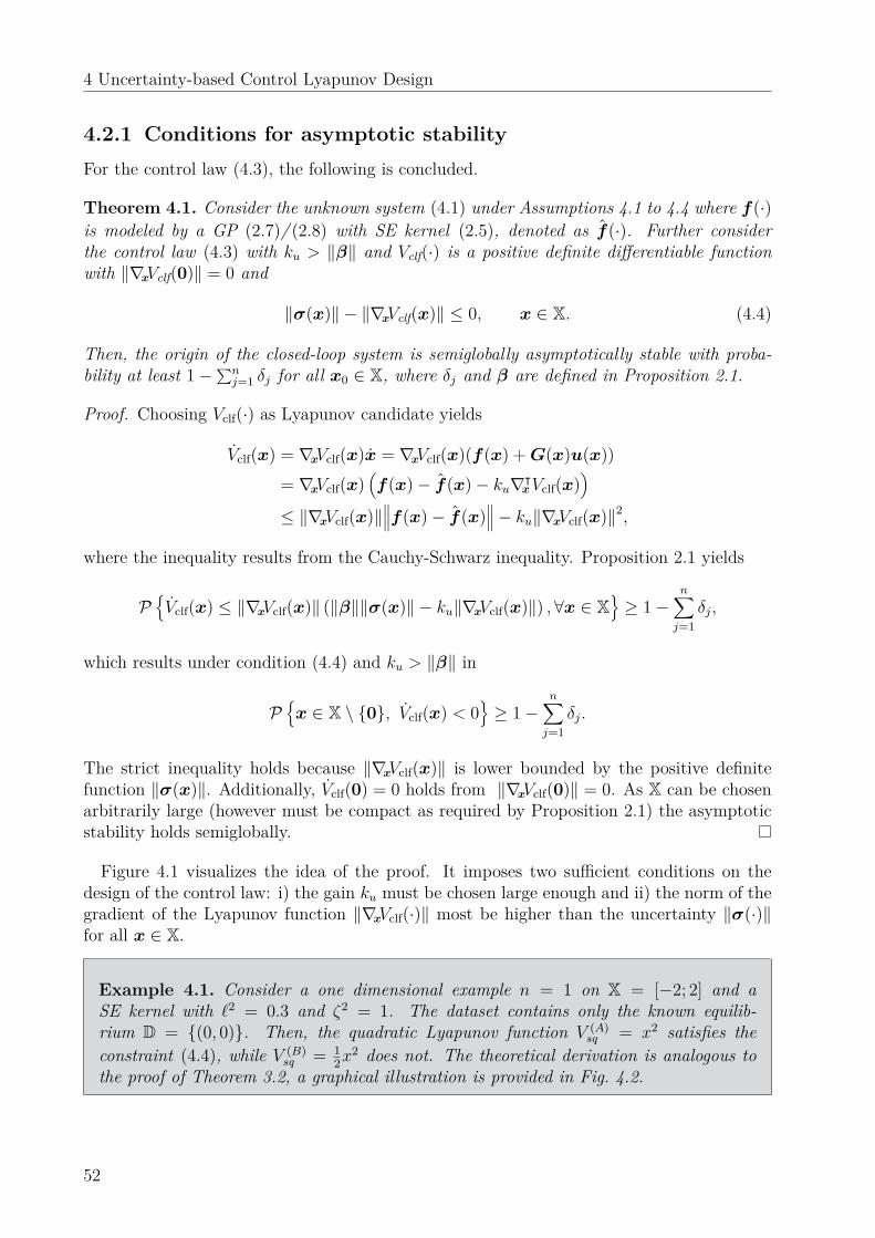
4 Uncertainty-based Control Lyapunov Design
4.2.1 Conditions for asymptotic stabilityFor the control law (4.3), the following is concluded.
Theorem 4.1. Consider the unknown system (4.1) under Assumptions 4.1 to 4.4 where f(·)is modeled by a GP (2.7)/ (2.8) with SE kernel (2.5), denoted as f(·). Further considerthe control law (4.3) with ku > ‖β‖ and Vclf(·) is a positive definite differentiable functionwith ‖∇xVclf(0)‖ = 0 and
‖σ(x)‖ − ‖∇xVclf(x)‖ ≤ 0, x ∈ X. (4.4)
Then, the origin of the closed-loop system is semiglobally asymptotically stable with proba-bility at least 1−∑n
j=1 δj for all x0 ∈ X, where δj and β are defined in Proposition 2.1.
Proof. Choosing Vclf(·) as Lyapunov candidate yields
Vclf(x) = ∇xVclf(x)x = ∇xVclf(x)(f(x) +G(x)u(x))= ∇xVclf(x)
(f(x)− f(x)− ku∇xᵀVclf(x)
)≤ ‖∇xVclf(x)‖
∥∥∥f(x)− f(x)∥∥∥− ku‖∇xVclf(x)‖2,
where the inequality results from the Cauchy-Schwarz inequality. Proposition 2.1 yields
PVclf(x) ≤ ‖∇xVclf(x)‖ (‖β‖‖σ(x)‖ − ku‖∇xVclf(x)‖) ,∀x ∈ X
≥ 1−
n∑j=1
δj,
which results under condition (4.4) and ku > ‖β‖ in
Px ∈ X \ 0, Vclf(x) < 0
≥ 1−
n∑j=1
δj.
The strict inequality holds because ‖∇xVclf(x)‖ is lower bounded by the positive definitefunction ‖σ(x)‖. Additionally, Vclf(0) = 0 holds from ‖∇xVclf(0)‖ = 0. As X can be chosenarbitrarily large (however must be compact as required by Proposition 2.1) the asymptoticstability holds semiglobally.
Figure 4.1 visualizes the idea of the proof. It imposes two sufficient conditions on thedesign of the control law: i) the gain ku must be chosen large enough and ii) the norm of thegradient of the Lyapunov function ‖∇xVclf(·)‖ most be higher than the uncertainty ‖σ(·)‖for all x ∈ X.
Example 4.1. Consider a one dimensional example n = 1 on X = [−2; 2] and aSE kernel with `2 = 0.3 and ζ2 = 1. The dataset contains only the known equilib-rium D = (0, 0). Then, the quadratic Lyapunov function V (A)
sq = x2 satisfies theconstraint (4.4), while V (B)
sq = 12x
2 does not. The theoretical derivation is analogous tothe proof of Theorem 3.2, a graphical illustration is provided in Fig. 4.2.
52
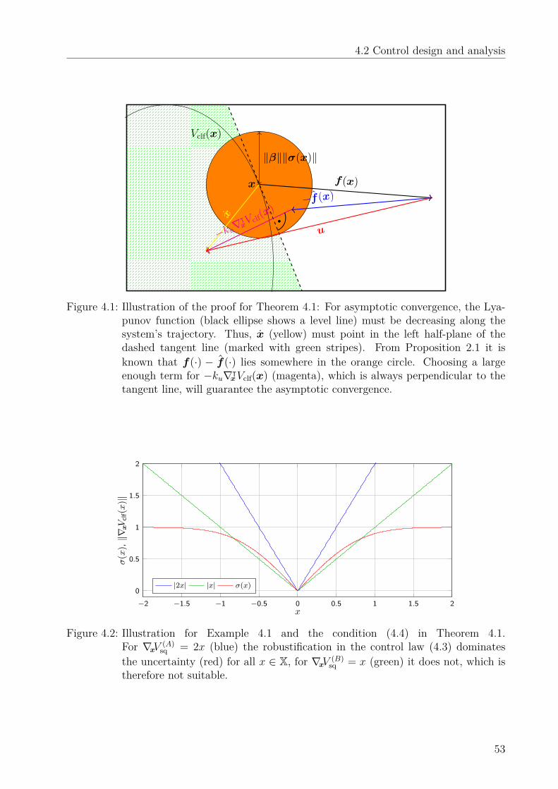
4.2 Control design and analysis
Vclf(x)
‖β‖‖σ(x)‖
x
x
f(x)−f(x)
−ku∇xᵀ Vclf(x
)
u
Figure 4.1: Illustration of the proof for Theorem 4.1: For asymptotic convergence, the Lya-punov function (black ellipse shows a level line) must be decreasing along thesystem’s trajectory. Thus, x (yellow) must point in the left half-plane of thedashed tangent line (marked with green stripes). From Proposition 2.1 it isknown that f(·) − f(·) lies somewhere in the orange circle. Choosing a largeenough term for −ku∇xᵀVclf(x) (magenta), which is always perpendicular to thetangent line, will guarantee the asymptotic convergence.
−2 −1.5 −1 −0.5 0 0.5 1 1.5 20
0.5
1
1.5
2
x
σ(x
),‖∇
xV
clf(x
)‖
|2x| |x| σ(x)
Figure 4.2: Illustration for Example 4.1 and the condition (4.4) in Theorem 4.1.For ∇xV (A)
sq = 2x (blue) the robustification in the control law (4.3) dominatesthe uncertainty (red) for all x ∈ X, for ∇xV (B)
sq = x (green) it does not, which istherefore not suitable.
53

4 Uncertainty-based Control Lyapunov Design
4.2.2 Optimality under power limitationsThe conditions for stability derived in Theorem 4.1 leave large freedom in the control designbecause there exists are variety of control Lyapunov functions which satisfy the requirements.In Example 4.1 the quadratic Lyapunov function with properly chosen parameters meetsthese requirements, but leads to unnecessary large control signals, in particular for |x| > 1(compare Fig. 4.2).Considering a power constraint in the control input
‖u(x)‖ ≤ umax, x ∈ X. (4.5)
the actuators can quickly saturate. Furthermore, the stability holds according to Theo-rem 4.1 only with a certain probability. It therefore desirable to make use of this freedom inthe design of Vclf(·) to optimize this reliability υ ∈ (0; 1), defined as υ := 1−∑n
j=1 δj.We introduce the notation β(υ) :=
∥∥∥[β1(δ1) · · · βn(δn)]ᵀ∥∥∥ and its corresponding in-
verse υ = b(β1, . . . , βn), which exists under the assumption δ = δ1 = δ2 = · · · = δn due tothe monotonicity of βj(δj), for j = 1, . . . ,n. Furthermore, we define
σ := maxx∈X‖σ(x)‖, µ := max
x∈X
∥∥∥f(x)∥∥∥, (4.6)
which exist due to the boundedness of the SE kernel. The smallest singular value of thematrix G(x), x ∈ X is denoted by %
G∈ R+,0.
This allows to find necessary conditions for the optimality of Vclf(·) and ku to maximizethe reliability υ under the power constraint (4.5).
Theorem 4.2. Assume umax > µ/%Gand consider the upper bound for the control input
‖u(x)‖ ≤ (µ+ ku‖∇xᵀVclf(x)‖)/%G≤ umax, x ∈ X. (4.7)
Then, the optimal reliability
υ∗ = arg max‖∇xVclf(x)‖,ku
υ (4.8a)
s.t. (µ+ ku‖∇xVclf(x)‖)/%G≤ umax, ku > β(υ),
‖∇xVclf(x)‖ ≥ ‖σ(x)‖, x ∈ X(4.8b)
is attained for
‖∇xVclf(x)‖ = ‖σ(x)‖, ku = (umax%G − µ)/σ + ε. (4.9)
for any arbitrarily small ε with (umax%G − µ)/σ > ε > 0. The maximum reliability is
υ∗ = b((umax%G − µ)/σ − ε
). (4.10)
Proof. The function β(υ) is monotone according to its definition in Proposition 2.1. Thisallows to reformulate the optimization as a maximization of β. The objective is then linearand the constraint set is convex. Thus, the maximum is attained on the boundary. As kumust not depend on x, but (4.8b) must hold ∀x ∈ X, the lower bound (umax%G − µ)/σ istaken for ku.
54
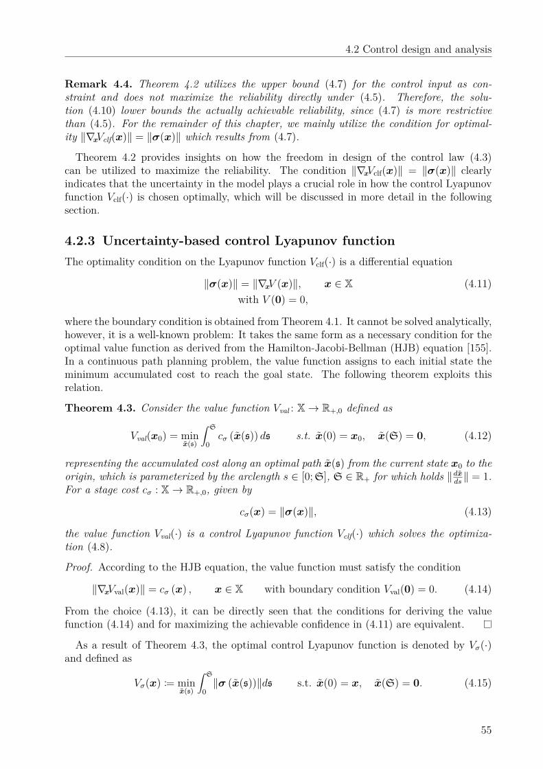
4.2 Control design and analysis
Remark 4.4. Theorem 4.2 utilizes the upper bound (4.7) for the control input as con-straint and does not maximize the reliability directly under (4.5). Therefore, the solu-tion (4.10) lower bounds the actually achievable reliability, since (4.7) is more restrictivethan (4.5). For the remainder of this chapter, we mainly utilize the condition for optimal-ity ‖∇xVclf(x)‖ = ‖σ(x)‖ which results from (4.7).
Theorem 4.2 provides insights on how the freedom in design of the control law (4.3)can be utilized to maximize the reliability. The condition ‖∇xVclf(x)‖ = ‖σ(x)‖ clearlyindicates that the uncertainty in the model plays a crucial role in how the control Lyapunovfunction Vclf(·) is chosen optimally, which will be discussed in more detail in the followingsection.
4.2.3 Uncertainty-based control Lyapunov functionThe optimality condition on the Lyapunov function Vclf(·) is a differential equation
‖σ(x)‖ = ‖∇xV (x)‖, x ∈ X (4.11)with V (0) = 0,
where the boundary condition is obtained from Theorem 4.1. It cannot be solved analytically,however, it is a well-known problem: It takes the same form as a necessary condition for theoptimal value function as derived from the Hamilton-Jacobi-Bellman (HJB) equation [155].In a continuous path planning problem, the value function assigns to each initial state theminimum accumulated cost to reach the goal state. The following theorem exploits thisrelation.
Theorem 4.3. Consider the value function Vval : X→ R+,0 defined as
Vval(x0) = minx(s)
∫ S
0cσ (x(s)) ds s.t. x(0) = x0, x(S) = 0, (4.12)
representing the accumulated cost along an optimal path x(s) from the current state x0 to theorigin, which is parameterized by the arclength s ∈ [0;S], S ∈ R+ for which holds ‖dx
ds‖ = 1.
For a stage cost cσ : X→ R+,0, given by
cσ(x) = ‖σ(x)‖, (4.13)
the value function Vval(·) is a control Lyapunov function Vclf(·) which solves the optimiza-tion (4.8).
Proof. According to the HJB equation, the value function must satisfy the condition
‖∇xVval(x)‖ = cσ (x) , x ∈ X with boundary condition Vval(0) = 0. (4.14)
From the choice (4.13), it can be directly seen that the conditions for deriving the valuefunction (4.14) and for maximizing the achievable confidence in (4.11) are equivalent.
As a result of Theorem 4.3, the optimal control Lyapunov function is denoted by Vσ(·)and defined as
Vσ(x) := minx(s)
∫ S
0‖σ (x(s))‖ds s.t. x(0) = x, x(S) = 0. (4.15)
55

4 Uncertainty-based Control Lyapunov Design
Remark 4.5. Equation (4.14) is also known as the inhomogeneous Eikonal equation [156].Even though its solution is for most cost functions not differentiable, [157] developed so-calledviscosity solutions. These exist for continuous, bounded and positive definite cost functions,which is fulfilled for the choice (4.13).
Remark 4.6. It can be concluded that there is an equivalence of the solution of the Eikonalequation (4.14) and the optimal control Lyapunov function which maximizes the reliability.From a practical perspective, this is helpful, since it allows to use existing tools from dynamicprogramming, e.g., fast marching methods [158] for efficient computation. From a theoreticalperspective, it verifies an intuitive understanding: By choosing the trajectory which minimizesthe uncertainty along the path, the reliability, the probability for asymptotic stability of theclosed-loop system is maximized.
Note that the control law (4.3) drives the system towards parts of the state space wherethe uncertainty is low and avoids areas with poor model quality. If the feedback linearizationwas perfect, the control law would track the optimal path (least accumulated uncertainty)based on the value function descend
x = −∇xVval(x).
As a summary of the results, the following proposition is stated.
Proposition 4.1. Consider the unknown system (4.1) under Assumptions 4.1 to 4.4 wherethe function f(·) is modeled by a GP (2.7)/ (2.8) with SE kernel (2.5), denoted as f(·)and the power constraint (4.7). Further consider the control law (4.3) where the gainis kc = (umax%G − µ)/σ + ε and Vclf(·) = Vσ(·) is a viscosity solution of (4.15). Then, theorigin of the closed-loop system is semiglobally asymptotically stable with at least probabilityυ∗ defined in Theorem 4.2.
Proof. The function Vσ(·) is positive definite from the fact that it is defined by a path integralover a positive definite cost function. The condition on Vσ(·) in (4.4) is fulfilled with equalityand kc > β(υ∗) holds from (4.10). Therefore, the stability follows directly from Theorem 4.1and the maximum confidence from Theorems 4.2 and 4.3.
4.2.4 Extension to other system classesWhile the main contribution of this chapter is derived for the fully actuated system in (4.1),we also provide some insight on how it can be extended to a more general system class.Consider a single-input control affine system in the canonical form
x1 = x2
x2 = x3
· · ·xn = f(x) + g(x)u, x0 = x(0), (4.16)
Equivalently to Assumptions 4.1 to 4.4 the following assumptions are made
Assumption 4.5. The function f : X→ R is unknown but the function value f(xg) isknown.
56
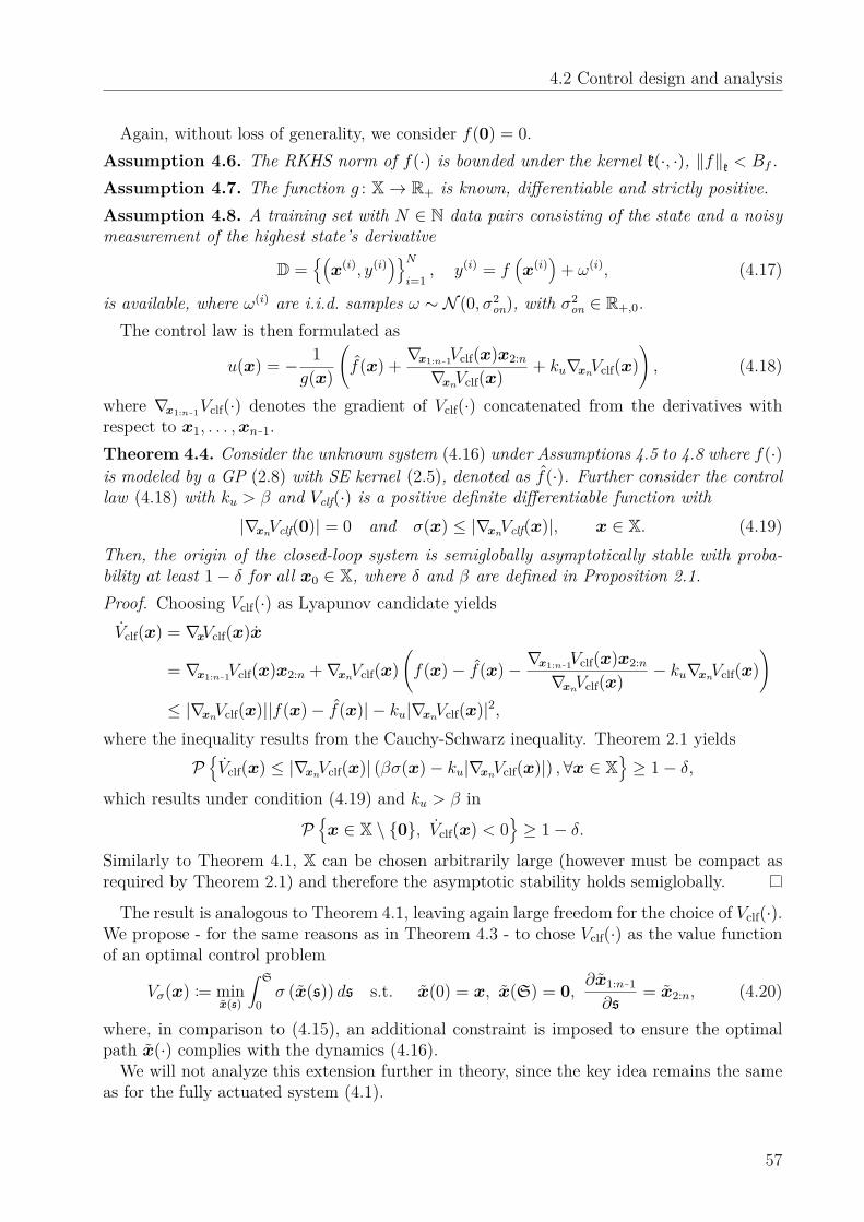
4.2 Control design and analysis
Again, without loss of generality, we consider f(0) = 0.Assumption 4.6. The RKHS norm of f(·) is bounded under the kernel k(·, ·), ‖f‖k < Bf .Assumption 4.7. The function g : X→ R+ is known, differentiable and strictly positive.Assumption 4.8. A training set with N ∈ N data pairs consisting of the state and a noisymeasurement of the highest state’s derivative
D =(x(i), y(i)
)Ni=1
, y(i) = f(x(i)
)+ ω(i), (4.17)
is available, where ω(i) are i.i.d. samples ω ∼ N (0,σ2on), with σ2
on ∈ R+,0.The control law is then formulated as
u(x) = − 1g(x)
(f(x) + ∇x1:n91Vclf(x)x2:n
∇xnVclf(x) + ku∇xnVclf(x))
, (4.18)
where ∇x1:n91Vclf(·) denotes the gradient of Vclf(·) concatenated from the derivatives withrespect to x1, . . . ,xn91.Theorem 4.4. Consider the unknown system (4.16) under Assumptions 4.5 to 4.8 where f(·)is modeled by a GP (2.8) with SE kernel (2.5), denoted as f(·). Further consider the controllaw (4.18) with ku > β and Vclf(·) is a positive definite differentiable function with
|∇xnVclf(0)| = 0 and σ(x) ≤ |∇xnVclf(x)|, x ∈ X. (4.19)Then, the origin of the closed-loop system is semiglobally asymptotically stable with proba-bility at least 1− δ for all x0 ∈ X, where δ and β are defined in Proposition 2.1.Proof. Choosing Vclf(·) as Lyapunov candidate yieldsVclf(x) = ∇xVclf(x)x
= ∇x1:n91Vclf(x)x2:n +∇xnVclf(x)(f(x)− f(x)− ∇x1:n91Vclf(x)x2:n
∇xnVclf(x) − ku∇xnVclf(x))
≤ |∇xnVclf(x)||f(x)− f(x)| − ku|∇xnVclf(x)|2,where the inequality results from the Cauchy-Schwarz inequality. Theorem 2.1 yields
PVclf(x) ≤ |∇xnVclf(x)| (βσ(x)− ku|∇xnVclf(x)|) ,∀x ∈ X
≥ 1− δ,
which results under condition (4.19) and ku > β in
Px ∈ X \ 0, Vclf(x) < 0
≥ 1− δ.
Similarly to Theorem 4.1, X can be chosen arbitrarily large (however must be compact asrequired by Theorem 2.1) and therefore the asymptotic stability holds semiglobally.
The result is analogous to Theorem 4.1, leaving again large freedom for the choice of Vclf(·).We propose - for the same reasons as in Theorem 4.3 - to chose Vclf(·) as the value functionof an optimal control problem
Vσ(x) := minx(s)
∫ S
0σ (x(s)) ds s.t. x(0) = x, x(S) = 0, ∂x1:n91
∂s= x2:n, (4.20)
where, in comparison to (4.15), an additional constraint is imposed to ensure the optimalpath x(·) complies with the dynamics (4.16).We will not analyze this extension further in theory, since the key idea remains the same
as for the fully actuated system (4.1).
57
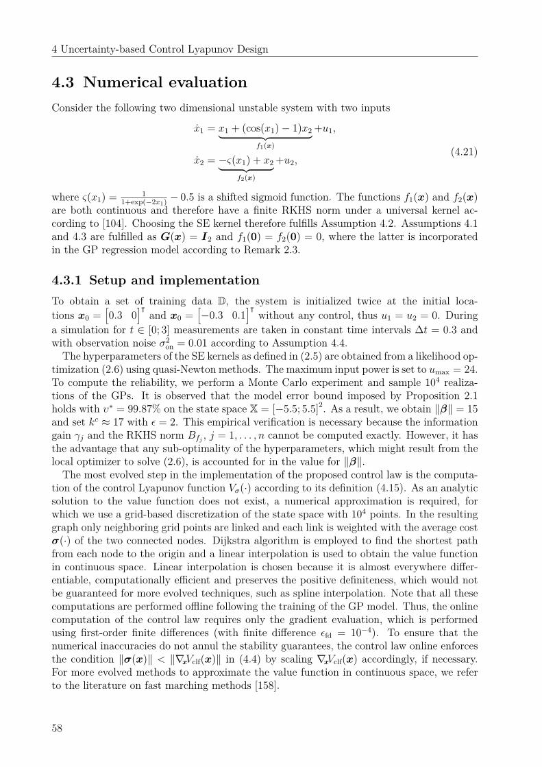
4 Uncertainty-based Control Lyapunov Design
4.3 Numerical evaluationConsider the following two dimensional unstable system with two inputs
x1 = x1 + (cos(x1)− 1)x2︸ ︷︷ ︸f1(x)
+u1,
x2 = −ς(x1) + x2︸ ︷︷ ︸f2(x)
+u2,(4.21)
where ς(x1) = 11+exp(−2x1) − 0.5 is a shifted sigmoid function. The functions f1(x) and f2(x)
are both continuous and therefore have a finite RKHS norm under a universal kernel ac-cording to [104]. Choosing the SE kernel therefore fulfills Assumption 4.2. Assumptions 4.1and 4.3 are fulfilled as G(x) = I2 and f1(0) = f2(0) = 0, where the latter is incorporatedin the GP regression model according to Remark 2.3.
4.3.1 Setup and implementationTo obtain a set of training data D, the system is initialized twice at the initial loca-tions x0 =
[0.3 0
]ᵀand x0 =
[−0.3 0.1
]ᵀwithout any control, thus u1 = u2 = 0. During
a simulation for t ∈ [0; 3] measurements are taken in constant time intervals ∆t = 0.3 andwith observation noise σ2
on = 0.01 according to Assumption 4.4.The hyperparameters of the SE kernels as defined in (2.5) are obtained from a likelihood op-
timization (2.6) using quasi-Newton methods. The maximum input power is set to umax = 24.To compute the reliability, we perform a Monte Carlo experiment and sample 104 realiza-tions of the GPs. It is observed that the model error bound imposed by Proposition 2.1holds with υ∗ = 99.87% on the state space X = [−5.5; 5.5]2. As a result, we obtain ‖β‖ = 15and set kc ≈ 17 with ε = 2. This empirical verification is necessary because the informationgain γj and the RKHS norm Bfj , j = 1, . . . ,n cannot be computed exactly. However, it hasthe advantage that any sub-optimality of the hyperparameters, which might result from thelocal optimizer to solve (2.6), is accounted for in the value for ‖β‖.The most evolved step in the implementation of the proposed control law is the computa-
tion of the control Lyapunov function Vσ(·) according to its definition (4.15). As an analyticsolution to the value function does not exist, a numerical approximation is required, forwhich we use a grid-based discretization of the state space with 104 points. In the resultinggraph only neighboring grid points are linked and each link is weighted with the average costσ(·) of the two connected nodes. Dijkstra algorithm is employed to find the shortest pathfrom each node to the origin and a linear interpolation is used to obtain the value functionin continuous space. Linear interpolation is chosen because it is almost everywhere differ-entiable, computationally efficient and preserves the positive definiteness, which would notbe guaranteed for more evolved techniques, such as spline interpolation. Note that all thesecomputations are performed offline following the training of the GP model. Thus, the onlinecomputation of the control law requires only the gradient evaluation, which is performedusing first-order finite differences (with finite difference εfd = 10−4). To ensure that thenumerical inaccuracies do not annul the stability guarantees, the control law online enforcesthe condition ‖σ(x)‖ < ‖∇xVclf(x)‖ in (4.4) by scaling ∇xVclf(x) accordingly, if necessary.For more evolved methods to approximate the value function in continuous space, we referto the literature on fast marching methods [158].
58
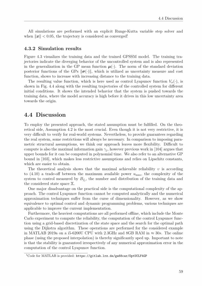
4.4 Discussion
All simulations are performed with an explicit Runge-Kutta variable step solver andwhen ‖x‖ < 0.05, the trajectory is considered as converged.1
4.3.2 Simulation resultsFigure 4.3 visualizes the training data and the trained GPSSM model. The training tra-jectories indicate the diverging behavior of the uncontrolled system and is also representedin the generalization in the GP mean function µ(·). The norm of the standard deviationposterior functions of the GPs ‖σ(·)‖, which is utilized as uncertainty measure and costfunction, shows to increase with increasing distance to the training data.The resulting value function, which is here used as control Lyapunov function Vσ(·), is
shown in Fig. 4.4 along with the resulting trajectories of the controlled system for differentinitial conditions. It shows the intended behavior that the system is pushed towards thetraining data, where the model accuracy is high before it drives in this low uncertainty areatowards the origin.
4.4 DiscussionTo employ the presented approach, the stated assumption must be fulfilled. On the theo-retical side, Assumption 4.2 is the most crucial. Even though it is not very restrictive, it isvery difficult to verify for real-world systems. Nevertheless, to provide guarantees regardingthe real system, some restrictions will always be necessary. In comparison to imposing para-metric structural assumptions, we think our approach leaves more flexibility. Difficult tocompute is also the maximal information gain γj, however previous work in [104] argues thatupper bounds for it can be computed in polynomial time. We also refer to an alternative GPbound in [103], which makes less restrictive assumptions and relies on Lipschitz constants,which are easier to obtain.The theoretical analysis shows that the maximal achievable reliability υ is according
to (4.10) a trade-off between the maximum available power umax, the complexity of thesystem to control measured by Bfj , the number and distribution of the training data andthe considered state space X.One major disadvantage on the practical side is the computational complexity of the ap-
proach. The control Lyapunov function cannot be computed analytically and the numericalapproximation techniques suffer from the curse of dimensionality. However, as we showequivalence to optimal control and dynamic programming problems, various techniques areapplicable to improve the current implementation.Furthermore, the heaviest computations are all performed offline, which include the Monte
Carlo experiment to compute the reliability, the computation of the control Lyapunov func-tion using a grid-based discretization of the state space and the search for the optimal pathusing the Dijkstra algorithm. These operations are performed for the considered examplein MATLAB 2019a on a i5-6200U CPU with 2.3GHz and 8GB RAM in ≈ 30s. The onlinephase (using the proposed interpolation) is thereby significantly sped up. Important to noteis that the stability is guaranteed irrespectively of any numerical approximation error in thecomputation of the control Lyapunov function.
1Code for MATLAB is provided: https://gitlab.lrz.de/ga68car/OptUCLF4GP
59
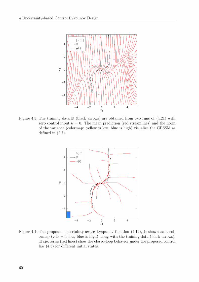
4 Uncertainty-based Control Lyapunov Design
−4 −2 0 2 4
−4
−2
0
2
4
x1
x2
‖σ(·)‖Dµ(·)
Figure 4.3: The training data D (black arrows) are obtained from two runs of (4.21) withzero control input u = 0. The mean prediction (red streamlines) and the normof the variance (colormap: yellow is low, blue is high) visualize the GPSSM asdefined in (2.7).
−4 −2 0 2 4
−4
−2
0
2
4
x1
x2
Vσ(·)Dx(t)
Figure 4.4: The proposed uncertainty-aware Lyapunov function (4.12), is shown as a col-ormap (yellow is low, blue is high) along with the training data (black arrows).Trajectories (red lines) show the closed-loop behavior under the proposed controllaw (4.3) for different initial states.
60

4.5 Summary
4.5 SummaryThis chapter proposes a control law to stabilize arbitrarily complex, unknown, fully actuatedsystems under mild assumptions with a specified probability. To achieve robustness tomodel uncertainties, the employed feedback linearization uses a control Lyapunov function.We first derive general conditions for asymptotic stability of the closed-loop system beforeproposing a specific uncertainty-based control Lyapunov function. We show that under apower constraint on the actuators, it yields the maximum reliability (probability to converge).This reveals an intuitive equivalence: Actively avoiding regions in the state space with lowmodel fidelity yields a controller which maximizes the probability of stability. This is notjust interesting from a theoretical perspective, but also comes with practical benefits as itallows to employ computational tools from path planning and dynamic programming.
61

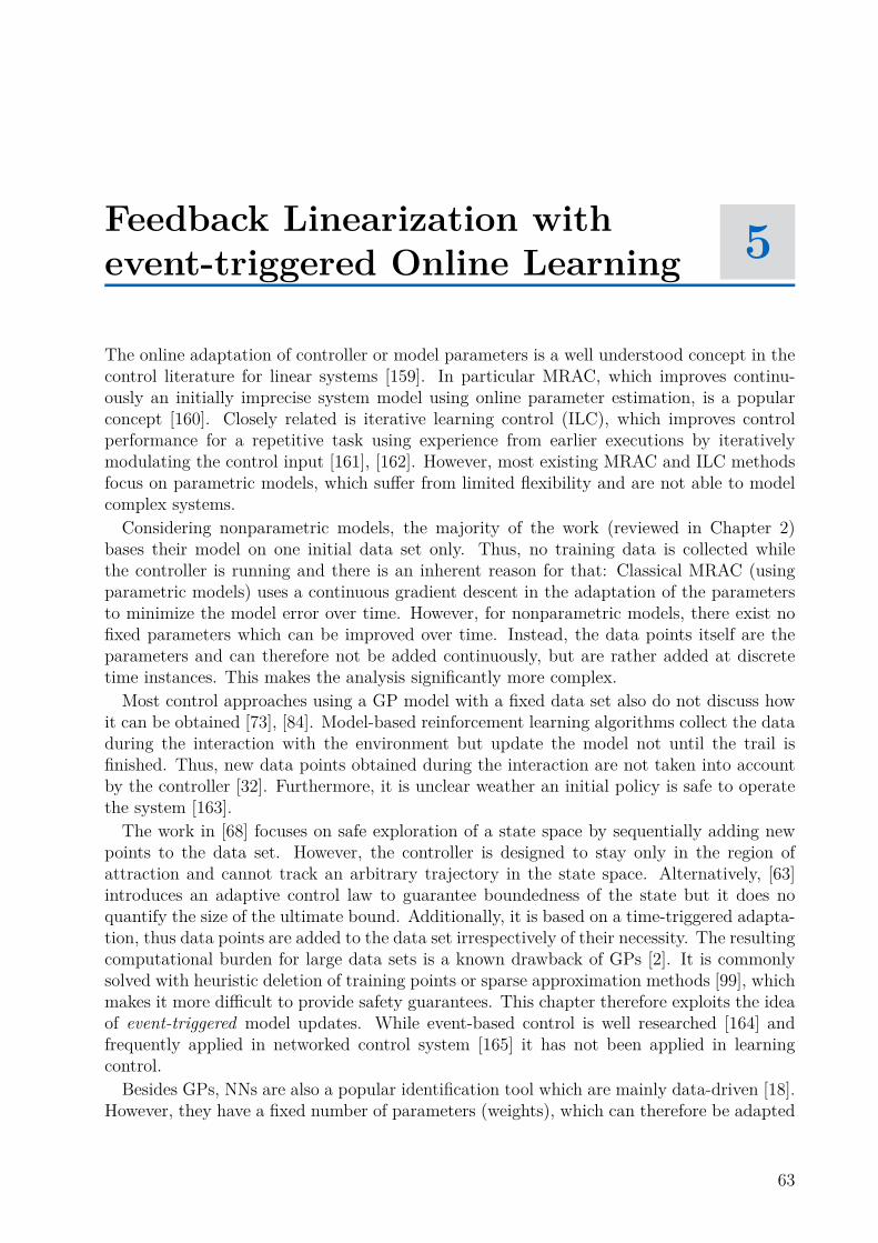
Feedback Linearization withevent-triggered Online Learning 5
The online adaptation of controller or model parameters is a well understood concept in thecontrol literature for linear systems [159]. In particular MRAC, which improves continu-ously an initially imprecise system model using online parameter estimation, is a popularconcept [160]. Closely related is iterative learning control (ILC), which improves controlperformance for a repetitive task using experience from earlier executions by iterativelymodulating the control input [161], [162]. However, most existing MRAC and ILC methodsfocus on parametric models, which suffer from limited flexibility and are not able to modelcomplex systems.Considering nonparametric models, the majority of the work (reviewed in Chapter 2)
bases their model on one initial data set only. Thus, no training data is collected whilethe controller is running and there is an inherent reason for that: Classical MRAC (usingparametric models) uses a continuous gradient descent in the adaptation of the parametersto minimize the model error over time. However, for nonparametric models, there exist nofixed parameters which can be improved over time. Instead, the data points itself are theparameters and can therefore not be added continuously, but are rather added at discretetime instances. This makes the analysis significantly more complex.Most control approaches using a GP model with a fixed data set also do not discuss how
it can be obtained [73], [84]. Model-based reinforcement learning algorithms collect the dataduring the interaction with the environment but update the model not until the trail isfinished. Thus, new data points obtained during the interaction are not taken into accountby the controller [32]. Furthermore, it is unclear weather an initial policy is safe to operatethe system [163].The work in [68] focuses on safe exploration of a state space by sequentially adding new
points to the data set. However, the controller is designed to stay only in the region ofattraction and cannot track an arbitrary trajectory in the state space. Alternatively, [63]introduces an adaptive control law to guarantee boundedness of the state but it does noquantify the size of the ultimate bound. Additionally, it is based on a time-triggered adapta-tion, thus data points are added to the data set irrespectively of their necessity. The resultingcomputational burden for large data sets is a known drawback of GPs [2]. It is commonlysolved with heuristic deletion of training points or sparse approximation methods [99], whichmakes it more difficult to provide safety guarantees. This chapter therefore exploits the ideaof event-triggered model updates. While event-based control is well researched [164] andfrequently applied in networked control system [165] it has not been applied in learningcontrol.Besides GPs, NNs are also a popular identification tool which are mainly data-driven [18].
However, they have a fixed number of parameters (weights), which can therefore be adapted
63
5 Feedback Linearization with event-triggered Online Learning
continuously over time as in MRAC. This allows [166], [167] and [168] to derive properstability and performance guarantees. Similarly, the work in [169] proposes a feedbacklinearizing control law and shows boundedness of the weights and the states in the closed-loop. However, it cannot quantify the ultimate bound because NNs, in contrast to GPs, donot inherently provide a measure for the precision of the model [170].This chapter’s major contribution is a novel nonparametric event-triggered online learning
control law, which guarantees stochastic asymptotic stability of initially unknown, controlaffine systems in the canonical form under very mild assumption. Its key idea is to add train-ing points, whenever the Lyapunov stability condition is in danger to be violated. We alsoaddress the challenge of constantly increasing computational complexity due to a growingdata set and propose a novel and safe data forgetting strategy for lifelong learning; It usesan information theoretic criterion to keep the most valuable points for tracking the futuredesired trajectory. The proposed control scheme is illustrated in Fig. 5.1.The chapter is based on the work published in [10], [11] and [12]. It is structured as follows:
After defining the problem setting in Sec. 5.1, this chapter proposes a GP-based closed-loopidentification in Sec. 5.2 and the control law in Sec. 5.3 including an analysis of the closed-loop behavior for model updates in arbitrary time instances. Section 5.4 introduces anevent-triggered model update for improved convergence and discusses strategies for efficientdata-handling. An evaluation in simulation and on a real-world robotic manipulator isprovided in Sec. 5.6, followed by a discussion in Sec. 5.7.
5.1 Problem formulationThis chapter considers a single-input control affine system in the canonical form
x1 = x2
x2 = x3
· · ·xn = f(x) + g(x)u, x0 = x(0), (5.1)
with state x =[x1 x2 · · · xn
]ᵀ ∈ X = Rn, input u ∈ U = R and unknown func-tions f : X→ R and g : X→ R. The following assumptions are made.Assumption 5.1. The unknown functions f(·) and g(·) are globally bounded and differen-tiable.Assuming the continuity is very natural for most physical systems and also boundedness
is often true in practical systems due to saturating effects or physical limits.Remark 5.1. The set X can also alternatively be considered as bounded, which automaticallyimplies (due to the differentiability) boundedness of f(·) and g(·). However, we decided X tobe unbounded and assume the dynamic functions to be bounded.With Assumption 5.1, the following is derived.
Lemma 5.1. Consider the system (5.1) under Assumption 5.1 with bounded and continuousinput u. Then, the solution x(t) does not have a finite escape time, thus @t∞, 0 < t∞ < ∞for which
limt→t∞‖x(t)‖ =∞.
64
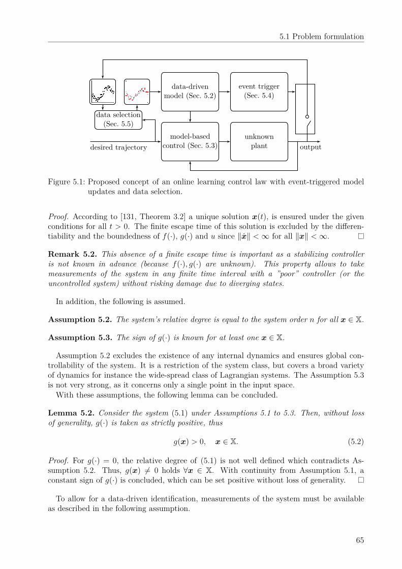
5.1 Problem formulation
unknownplant
model-basedcontrol (Sec. 5.3)
data-drivenmodel (Sec. 5.2)
event trigger(Sec. 5.4)
data selection(Sec. 5.5)
desired trajectory output
Figure 5.1: Proposed concept of an online learning control law with event-triggered modelupdates and data selection.
Proof. According to [131, Theorem 3.2] a unique solution x(t), is ensured under the givenconditions for all t > 0. The finite escape time of this solution is excluded by the differen-tiability and the boundedness of f(·), g(·) and u since ‖x‖ <∞ for all ‖x‖ <∞.
Remark 5.2. This absence of a finite escape time is important as a stabilizing controlleris not known in advance (because f(·), g(·) are unknown). This property allows to takemeasurements of the system in any finite time interval with a ”poor” controller (or theuncontrolled system) without risking damage due to diverging states.
In addition, the following is assumed.
Assumption 5.2. The system’s relative degree is equal to the system order n for all x ∈ X.
Assumption 5.3. The sign of g(·) is known for at least one x ∈ X.
Assumption 5.2 excludes the existence of any internal dynamics and ensures global con-trollability of the system. It is a restriction of the system class, but covers a broad varietyof dynamics for instance the wide-spread class of Lagrangian systems. The Assumption 5.3is not very strong, as it concerns only a single point in the input space.With these assumptions, the following lemma can be concluded.
Lemma 5.2. Consider the system (5.1) under Assumptions 5.1 to 5.3. Then, without lossof generality, g(·) is taken as strictly positive, thus
g(x) > 0, x ∈ X. (5.2)
Proof. For g(·) = 0, the relative degree of (5.1) is not well defined which contradicts As-sumption 5.2. Thus, g(x) 6= 0 holds ∀x ∈ X. With continuity from Assumption 5.1, aconstant sign of g(·) is concluded, which can be set positive without loss of generality.
To allow for a data-driven identification, measurements of the system must be availableas described in the following assumption.
65
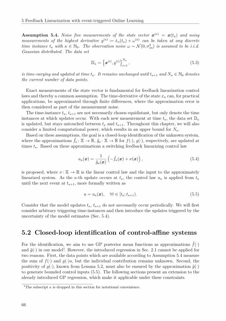
5 Feedback Linearization with event-triggered Online Learning
Assumption 5.4. Noise free measurements of the state vector x(κ) = x(tκ) and noisymeasurements of the highest derivative y(κ) := xn(tκ) + ω(κ) can be taken at any discretetime instance tκ with κ ∈ N0. The observation noise ω ∼ N (0,σ2
on) is assumed to be i.i.d.Gaussian distributed. The data set
Dκ =x(i), y(i)
Nκi=1
, (5.3)
is time-varying and updated at time tκ. It remains unchanged until tκ+1 and Nκ ∈ N0 denotesthe current number of data points.
Exact measurements of the state vector is fundamental for feedback linearization controllaws and thereby a common assumption. The time-derivative of the state xn can, for practicalapplications, be approximated through finite differences, where the approximation error isthen considered as part of the measurement noise.The time-instance tκ, tκ+1 are not necessarily chosen equidistant, but only denote the time
instances at which updates occur. With each new measurement at time tκ, the data set Dκ
is updated, but stays untouched between tκ and tκ+1. Throughout this chapter, we will alsoconsider a limited computational power, which results in an upper bound for Nκ.Based on these assumptions, the goal is a closed-loop identification of the unknown system,
where the approximations fκ : X→ R, gκ : X→ R for f(·), g(·), respectively, are updated attimes tκ. Based on these approximations a switching feedback linearizing control law
uκ(x) = 1gκ(x)
(−fκ(x) + ν(x)
), (5.4)
is proposed, where ν : X → R is the linear control law and the input to the approximatelylinearized system. As the κ-th update occurs at tκ, the control law uκ is applied from tκuntil the next event at tκ+1, more formally written as
u = uκ(x), ∀t ∈ [tκ; tκ+1). (5.5)
Consider that the model updates tκ, tκ+1 do not necessarily occur periodically. We will firstconsider arbitrary triggering time-instances and then introduce the updates triggered by theuncertainty of the model estimates (Sec. 5.4).
5.2 Closed-loop identification of control-affine systems
For the identification, we aim to use GP posterior mean functions as approximations f(·)and g(·) in our model1. However, the introduced regression in Sec. 2.1 cannot be applied fortwo reasons. First, the data points which are available according to Assumption 5.4 measurethe sum of f(·) and g(·)u, but the individual contribution remains unknown. Second, thepositivity of g(·), known from Lemma 5.2, must also be ensured by the approximation g(·)to generate bounded control inputs (5.5). The following sections present an extension to thealready introduced GP regression, which make it applicable under these constraints.
1The subscript κ is dropped in this section for notational convenience.
66
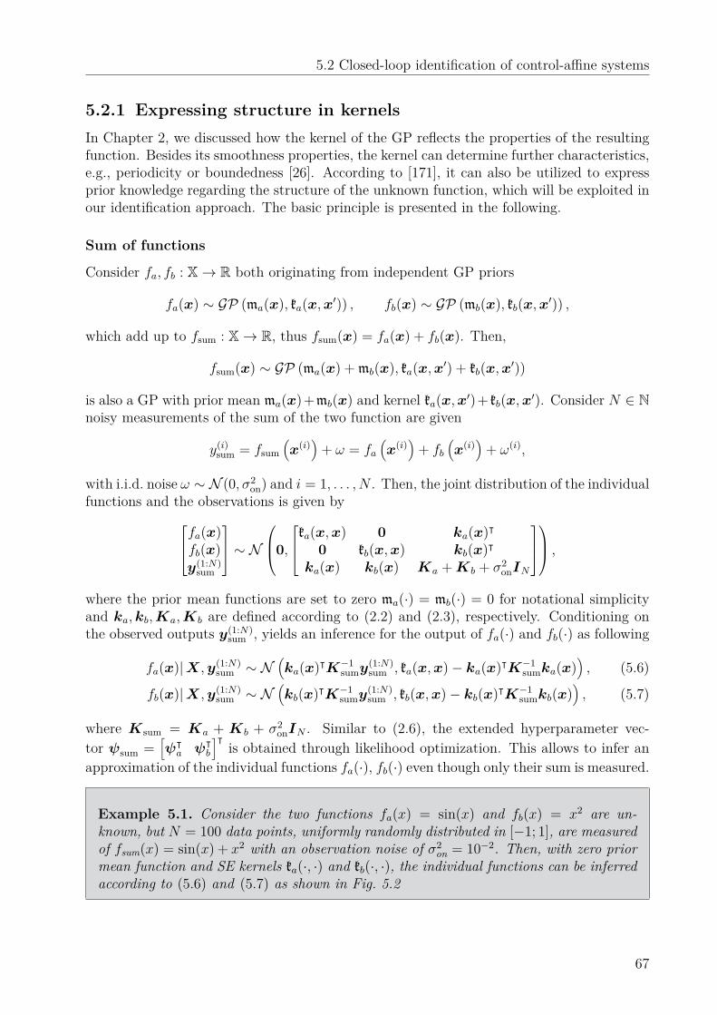
5.2 Closed-loop identification of control-affine systems
5.2.1 Expressing structure in kernelsIn Chapter 2, we discussed how the kernel of the GP reflects the properties of the resultingfunction. Besides its smoothness properties, the kernel can determine further characteristics,e.g., periodicity or boundedness [26]. According to [171], it can also be utilized to expressprior knowledge regarding the structure of the unknown function, which will be exploited inour identification approach. The basic principle is presented in the following.
Sum of functions
Consider fa, fb : X→ R both originating from independent GP priors
fa(x) ∼ GP (ma(x), ka(x,x′)) , fb(x) ∼ GP (mb(x), kb(x,x′)) ,
which add up to fsum : X→ R, thus fsum(x) = fa(x) + fb(x). Then,
fsum(x) ∼ GP (ma(x) + mb(x), ka(x,x′) + kb(x,x′))
is also a GP with prior mean ma(x)+mb(x) and kernel ka(x,x′)+ kb(x,x′). Consider N ∈ Nnoisy measurements of the sum of the two function are given
y(i)sum = fsum
(x(i)
)+ ω = fa
(x(i)
)+ fb
(x(i)
)+ ω(i),
with i.i.d. noise ω ∼ N (0,σ2on) and i = 1, . . . ,N . Then, the joint distribution of the individual
functions and the observations is given byfa(x)fb(x)y(1:N)
sum
∼ N0,
ka(x,x) 0 ka(x)ᵀ0 kb(x,x) kb(x)ᵀ
ka(x) kb(x) Ka +Kb + σ2onIN
,
where the prior mean functions are set to zero ma(·) = mb(·) = 0 for notational simplicityand ka,kb,Ka,Kb are defined according to (2.2) and (2.3), respectively. Conditioning onthe observed outputs y(1:N)
sum , yields an inference for the output of fa(·) and fb(·) as following
fa(x)|X,y(1:N)sum ∼ N
(ka(x)ᵀK−1
sumy(1:N)sum , ka(x,x)− ka(x)ᵀK−1
sumka(x))
, (5.6)
fb(x)|X,y(1:N)sum ∼ N
(kb(x)ᵀK−1
sumy(1:N)sum , kb(x,x)− kb(x)ᵀK−1
sumkb(x))
, (5.7)
where Ksum = Ka + Kb + σ2onIN . Similar to (2.6), the extended hyperparameter vec-
tor ψsum =[ψᵀa ψᵀ
b
]ᵀis obtained through likelihood optimization. This allows to infer an
approximation of the individual functions fa(·), fb(·) even though only their sum is measured.
Example 5.1. Consider the two functions fa(x) = sin(x) and fb(x) = x2 are un-known, but N = 100 data points, uniformly randomly distributed in [−1; 1], are measuredof fsum(x) = sin(x) + x2 with an observation noise of σ2
on = 10−2. Then, with zero priormean function and SE kernels ka(·, ·) and kb(·, ·), the individual functions can be inferredaccording to (5.6) and (5.7) as shown in Fig. 5.2
67
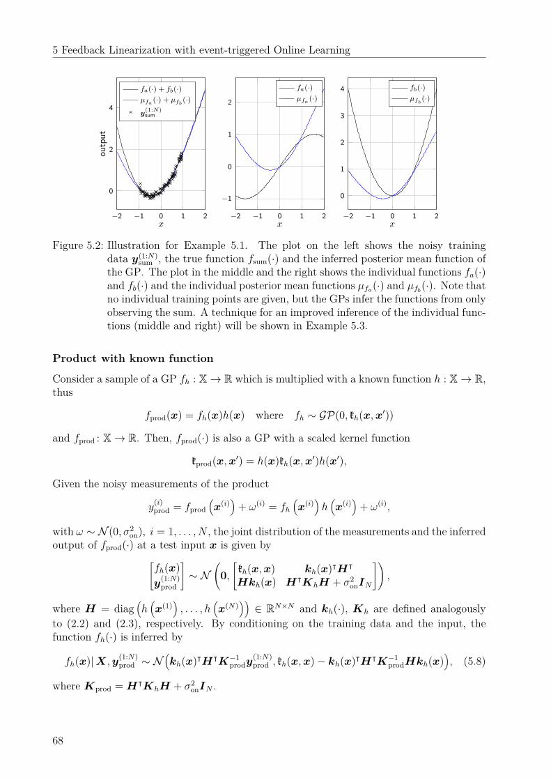
5 Feedback Linearization with event-triggered Online Learning
−2 −1 0 1 2
0
2
4
x
outp
utfa(·) + fb(·)µfa (·) + µfb
(·)y
(1:N)sum
−2 −1 0 1 2
−1
0
1
2
x
fa(·)µfa (·)
−2 −1 0 1 2
0
1
2
3
4
x
fb(·)µfb
(·)
Figure 5.2: Illustration for Example 5.1. The plot on the left shows the noisy trainingdata y(1:N)
sum , the true function fsum(·) and the inferred posterior mean function ofthe GP. The plot in the middle and the right shows the individual functions fa(·)and fb(·) and the individual posterior mean functions µfa(·) and µfb(·). Note thatno individual training points are given, but the GPs infer the functions from onlyobserving the sum. A technique for an improved inference of the individual func-tions (middle and right) will be shown in Example 5.3.
Product with known function
Consider a sample of a GP fh : X→ R which is multiplied with a known function h : X→ R,thus
fprod(x) = fh(x)h(x) where fh ∼ GP(0, kh(x,x′))
and fprod : X→ R. Then, fprod(·) is also a GP with a scaled kernel function
kprod(x,x′) = h(x)kh(x,x′)h(x′),
Given the noisy measurements of the product
y(i)prod = fprod
(x(i)
)+ ω(i) = fh
(x(i)
)h(x(i)
)+ ω(i),
with ω ∼ N (0,σ2on), i = 1, . . . ,N , the joint distribution of the measurements and the inferred
output of fprod(·) at a test input x is given by[fh(x)y
(1:N)prod
]∼ N
(0,[kh(x,x) kh(x)ᵀHᵀ
Hkh(x) HᵀKhH + σ2onIN
]),
where H = diag(h(x(1)
), . . . ,h
(x(N)
))∈ RN×N and kh(·), Kh are defined analogously
to (2.2) and (2.3), respectively. By conditioning on the training data and the input, thefunction fh(·) is inferred by
fh(x)|X,y(1:N)prod ∼ N
(kh(x)ᵀHᵀK−1
prody(1:N)prod , kh(x,x)− kh(x)ᵀHᵀK−1
prodHkh(x)), (5.8)
where Kprod = HᵀKhH + σ2onIN .
68
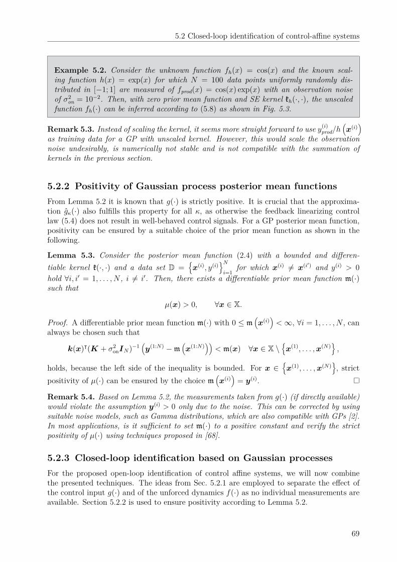
5.2 Closed-loop identification of control-affine systems
Example 5.2. Consider the unknown function fh(x) = cos(x) and the known scal-ing function h(x) = exp(x) for which N = 100 data points uniformly randomly dis-tributed in [−1; 1] are measured of fprod(x) = cos(x) exp(x) with an observation noiseof σ2
on = 10−2. Then, with zero prior mean function and SE kernel kh(·, ·), the unscaledfunction fh(·) can be inferred according to (5.8) as shown in Fig. 5.3.
Remark 5.3. Instead of scaling the kernel, it seems more straight forward to use y(i)prod/h
(x(i)
)as training data for a GP with unscaled kernel. However, this would scale the observationnoise undesirably, is numerically not stable and is not compatible with the summation ofkernels in the previous section.
5.2.2 Positivity of Gaussian process posterior mean functionsFrom Lemma 5.2 it is known that g(·) is strictly positive. It is crucial that the approxima-tion gκ(·) also fulfills this property for all κ, as otherwise the feedback linearizing controllaw (5.4) does not result in well-behaved control signals. For a GP posterior mean function,positivity can be ensured by a suitable choice of the prior mean function as shown in thefollowing.
Lemma 5.3. Consider the posterior mean function (2.4) with a bounded and differen-tiable kernel k(·, ·) and a data set D =
x(i), y(i)
Ni=1
for which x(i) 6= x(i′) and y(i) > 0hold ∀i, i′ = 1, . . . ,N , i 6= i′. Then, there exists a differentiable prior mean function m(·)such that
µ(x) > 0, ∀x ∈ X.
Proof. A differentiable prior mean function m(·) with 0 ≤ m(x(i)
)<∞, ∀i = 1, . . . ,N , can
always be chosen such that
k(x)ᵀ(K + σ2onIN)−1
(y(1:N) −m
(x(1:N)
))< m(x) ∀x ∈ X \
x(1), . . . ,x(N)
,
holds, because the left side of the inequality is bounded. For x ∈x(1), . . . ,x(N)
, strict
positivity of µ(·) can be ensured by the choice m(x(i)
)= y(i).
Remark 5.4. Based on Lemma 5.2, the measurements taken from g(·) (if directly available)would violate the assumption y(i) > 0 only due to the noise. This can be corrected by usingsuitable noise models, such as Gamma distributions, which are also compatible with GPs [2].In most applications, is it sufficient to set m(·) to a positive constant and verify the strictpositivity of µ(·) using techniques proposed in [68].
5.2.3 Closed-loop identification based on Gaussian processesFor the proposed open-loop identification of control affine systems, we will now combinethe presented techniques. The ideas from Sec. 5.2.1 are employed to separate the effect ofthe control input g(·) and of the unforced dynamics f(·) as no individual measurements areavailable. Section 5.2.2 is used to ensure positivity according to Lemma 5.2.
69
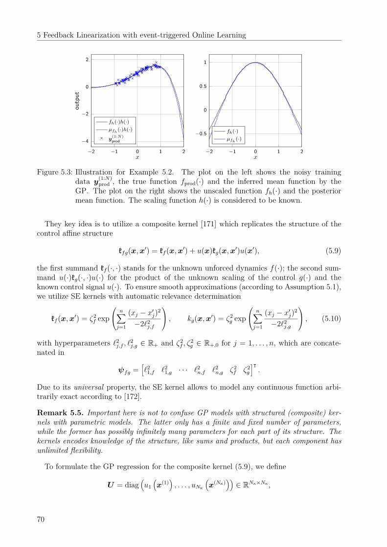
5 Feedback Linearization with event-triggered Online Learning
−2 −1 0 1 2
−4
−2
0
2
x
outp
ut
fh(·)h(·)µfh
(·)h(·)y
(1:N)prod
−2 −1 0 1 2
−0.5
0
0.5
1
x
fh(·)µfh
(·)
Figure 5.3: Illustration for Example 5.2. The plot on the left shows the noisy trainingdata y(1:N)
prod , the true function fprod(·) and the inferred mean function by theGP. The plot on the right shows the unscaled function fh(·) and the posteriormean function. The scaling function h(·) is considered to be known.
They key idea is to utilize a composite kernel [171] which replicates the structure of thecontrol affine structure
kfg(x,x′) = kf (x,x′) + u(x)kg(x,x′)u(x′), (5.9)
the first summand kf (·, ·) stands for the unknown unforced dynamics f(·); the second sum-mand u(·)kg(·, ·)u(·) for the product of the unknown scaling of the control g(·) and theknown control signal u(·). To ensure smooth approximations (according to Assumption 5.1),we utilize SE kernels with automatic relevance determination
kf (x,x′) = ζ2f exp
n∑j=1
(xj − x′j)2
−2`2j,f
, kg(x,x′) = ζ2g exp
n∑j=1
(xj − x′j)2
−2`2j,g
, (5.10)
with hyperparameters `2j,f , `2
j,g ∈ R+ and ζ2f , ζ2
g ∈ R+,0 for j = 1, . . . ,n, which are concate-nated in
ψfg =[`2
1,f `21,g · · · `2
n,f `2n,g ζ2
f ζ2g
]ᵀ.
Due to its universal property, the SE kernel allows to model any continuous function arbi-trarily exact according to [172].
Remark 5.5. Important here is not to confuse GP models with structured (composite) ker-nels with parametric models. The latter only has a finite and fixed number of parameters,while the former has possibly infinitely many parameters for each part of its structure. Thekernels encodes knowledge of the structure, like sums and products, but each component hasunlimited flexibility.
To formulate the GP regression for the composite kernel (5.9), we define
U = diag(u1(x(1)
), . . . ,uNκ
(x(Nκ)
))∈ RNκ×Nκ ,
70
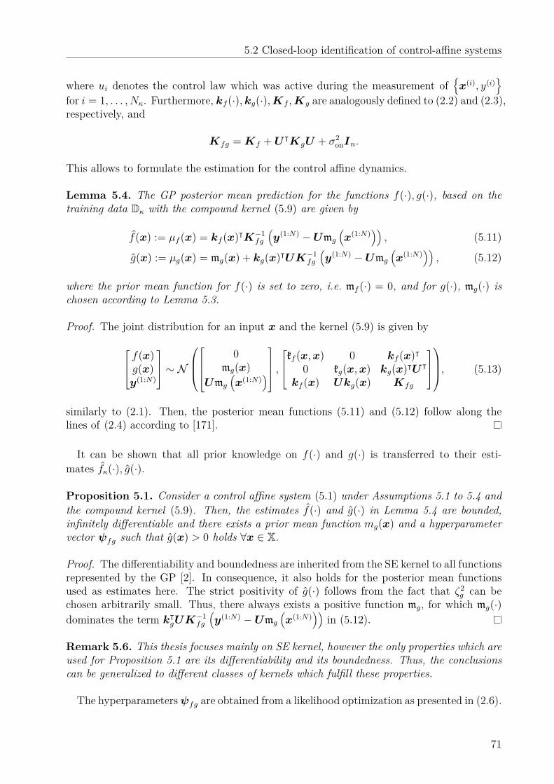
5.2 Closed-loop identification of control-affine systems
where ui denotes the control law which was active during the measurement ofx(i), y(i)
for i = 1, . . . ,Nκ. Furthermore, kf (·),kg(·),Kf ,Kg are analogously defined to (2.2) and (2.3),respectively, and
Kfg = Kf +U ᵀKgU + σ2onIn.
This allows to formulate the estimation for the control affine dynamics.
Lemma 5.4. The GP posterior mean prediction for the functions f(·), g(·), based on thetraining data Dκ with the compound kernel (5.9) are given by
f(x) := µf (x) = kf (x)ᵀK−1fg
(y(1:N) −Umg
(x(1:N)
)), (5.11)
g(x) := µg(x) = mg(x) + kg(x)ᵀUK−1fg
(y(1:N) −Umg
(x(1:N)
)), (5.12)
where the prior mean function for f(·) is set to zero, i.e. mf (·) = 0, and for g(·), mg(·) ischosen according to Lemma 5.3.
Proof. The joint distribution for an input x and the kernel (5.9) is given by
f(x)g(x)y(1:N)
∼ N
0mg(x)
Umg
(x(1:N)
) ,
kf (x,x) 0 kf (x)ᵀ0 kg(x,x) kg(x)ᵀU ᵀ
kf (x) Ukg(x) Kfg
, (5.13)
similarly to (2.1). Then, the posterior mean functions (5.11) and (5.12) follow along thelines of (2.4) according to [171].
It can be shown that all prior knowledge on f(·) and g(·) is transferred to their esti-mates fκ(·), g(·).
Proposition 5.1. Consider a control affine system (5.1) under Assumptions 5.1 to 5.4 andthe compound kernel (5.9). Then, the estimates f(·) and g(·) in Lemma 5.4 are bounded,infinitely differentiable and there exists a prior mean function mg(x) and a hyperparametervector ψfg such that g(x) > 0 holds ∀x ∈ X.
Proof. The differentiability and boundedness are inherited from the SE kernel to all functionsrepresented by the GP [2]. In consequence, it also holds for the posterior mean functionsused as estimates here. The strict positivity of g(·) follows from the fact that ζ2
g can bechosen arbitrarily small. Thus, there always exists a positive function mg, for which mg(·)dominates the term kᵀ
gUK−1fg
(y(1:N) −Umg
(x(1:N)
))in (5.12).
Remark 5.6. This thesis focuses mainly on SE kernel, however the only properties which areused for Proposition 5.1 are its differentiability and its boundedness. Thus, the conclusionscan be generalized to different classes of kernels which fulfill these properties.
The hyperparametersψfg are obtained from a likelihood optimization as presented in (2.6).
71
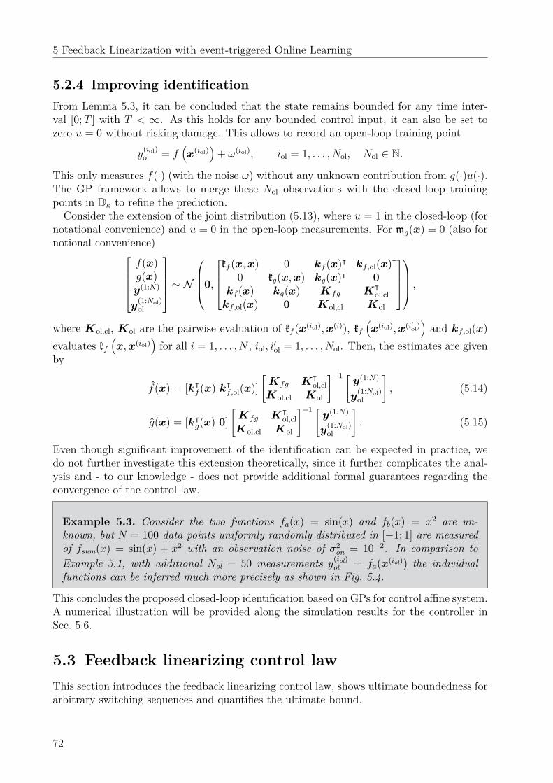
5 Feedback Linearization with event-triggered Online Learning
5.2.4 Improving identificationFrom Lemma 5.3, it can be concluded that the state remains bounded for any time inter-val [0;T ] with T < ∞. As this holds for any bounded control input, it can also be set tozero u = 0 without risking damage. This allows to record an open-loop training point
y(iol)ol = f
(x(iol)
)+ ω(iol), iol = 1, . . . ,Nol, Nol ∈ N.
This only measures f(·) (with the noise ω) without any unknown contribution from g(·)u(·).The GP framework allows to merge these Nol observations with the closed-loop trainingpoints in Dκ to refine the prediction.Consider the extension of the joint distribution (5.13), where u = 1 in the closed-loop (for
notational convenience) and u = 0 in the open-loop measurements. For mg(x) = 0 (also fornotional convenience)
f(x)g(x)y(1:N)
y(1:Nol)ol
∼ N0,
kf (x,x) 0 kf (x)ᵀ kf ,ol(x)ᵀ
0 kg(x,x) kg(x)ᵀ 0kf (x) kg(x) Kfg Kᵀ
ol,clkf ,ol(x) 0 Kol,cl Kol
,
where Kol,cl, Kol are the pairwise evaluation of kf (x(iol),x(i)), kf(x(iol),x(i′ol)
)and kf ,ol(x)
evaluates kf(x,x(iol)
)for all i = 1, . . . ,N , iol, i′ol = 1, . . . ,Nol. Then, the estimates are given
by
f(x) = [kᵀf (x) kᵀ
f ,ol(x)][Kfg Kᵀ
ol,clKol,cl Kol
]−1 [y(1:N)
y(1:Nol)ol
], (5.14)
g(x) = [kᵀg(x) 0]
[Kfg Kᵀ
ol,clKol,cl Kol
]−1 [y(1:N)
y(1:Nol)ol
]. (5.15)
Even though significant improvement of the identification can be expected in practice, wedo not further investigate this extension theoretically, since it further complicates the anal-ysis and - to our knowledge - does not provide additional formal guarantees regarding theconvergence of the control law.
Example 5.3. Consider the two functions fa(x) = sin(x) and fb(x) = x2 are un-known, but N = 100 data points uniformly randomly distributed in [−1; 1] are measuredof fsum(x) = sin(x) + x2 with an observation noise of σ2
on = 10−2. In comparison toExample 5.1, with additional Nol = 50 measurements y(iol)
ol = fa(x(iol)) the individualfunctions can be inferred much more precisely as shown in Fig. 5.4.
This concludes the proposed closed-loop identification based on GPs for control affine system.A numerical illustration will be provided along the simulation results for the controller inSec. 5.6.
5.3 Feedback linearizing control lawThis section introduces the feedback linearizing control law, shows ultimate boundedness forarbitrary switching sequences and quantifies the ultimate bound.
72
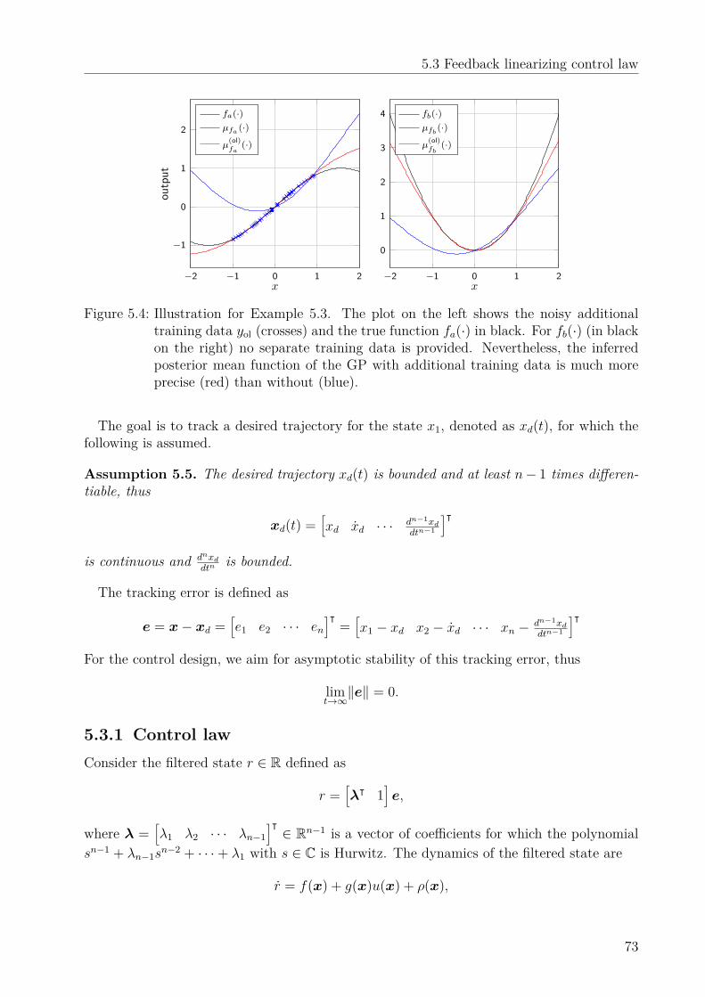
5.3 Feedback linearizing control law
−2 −1 0 1 2
−1
0
1
2
x
outp
ut
fa(·)µfa (·)µ
(ol)fa
(·)
−2 −1 0 1 2
0
1
2
3
4
x
fb(·)µfb
(·)µ
(ol)fb
(·)
Figure 5.4: Illustration for Example 5.3. The plot on the left shows the noisy additionaltraining data yol (crosses) and the true function fa(·) in black. For fb(·) (in blackon the right) no separate training data is provided. Nevertheless, the inferredposterior mean function of the GP with additional training data is much moreprecise (red) than without (blue).
The goal is to track a desired trajectory for the state x1, denoted as xd(t), for which thefollowing is assumed.
Assumption 5.5. The desired trajectory xd(t) is bounded and at least n− 1 times differen-tiable, thus
xd(t) =[xd xd · · · dn−1xd
dtn−1
]ᵀis continuous and dnxd
dtnis bounded.
The tracking error is defined as
e = x− xd =[e1 e2 · · · en
]ᵀ=[x1 − xd x2 − xd · · · xn − dn−1xd
dtn−1
]ᵀFor the control design, we aim for asymptotic stability of this tracking error, thus
limt→∞‖e‖ = 0.
5.3.1 Control lawConsider the filtered state r ∈ R defined as
r =[λᵀ 1
]e,
where λ =[λ1 λ2 · · · λn−1
]ᵀ ∈ Rn−1 is a vector of coefficients for which the polynomialsn−1 + λn−1s
n−2 + · · ·+ λ1 with s ∈ C is Hurwitz. The dynamics of the filtered state are
r = f(x) + g(x)u(x) + ρ(x),
73
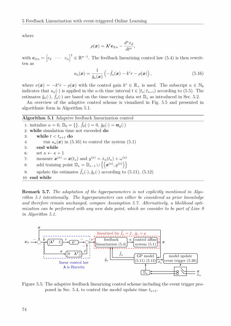
5 Feedback Linearization with event-triggered Online Learning
where
ρ(x) = λᵀe2:n −dnxddtn
,
with e2:n =[e2 · · · en
]ᵀ ∈ Rn−1. The feedback linearizing control law (5.4) is then rewrit-ten as
uκ(x) = 1gκ(x)
(−fκ(x)− kcr − ρ(x)
), (5.16)
where ν(x) = −kcr − ρ(x) with the control gain kc ∈ R+ is used. The subscript κ ∈ N0indicates that uκ(·) is applied in the κ-th time interval t ∈ [tκ; tκ+1) according to (5.5). Theestimates gκ(·), fκ(·) are based on the time-varying data set Dκ as introduced in Sec. 5.2.An overview of the adaptive control scheme is visualized in Fig. 5.5 and presented in
algorithmic form in Algorithm 5.1.
Algorithm 5.1 Adaptive feedback linearization control1: initialize κ = 0, D0 = , f0(·) = 0, g0(·) = mg(·)2: while simulation time not exceeded do3: while t < tκ+1 do4: run uκ(x) in (5.16) to control the system (5.1)5: end while6: set κ← κ+ 17: measure x(κ) = x(tκ) and y(κ) = xn(tκ) + ω(κ)
8: add training point Dκ = Dκ−1 ∪(x(κ), y(κ)
)9: update the estimates fκ(·), gκ(·) according to (5.11), (5.12)10: end while
Remark 5.7. The adaptation of the hyperparameters is not explicitly mentioned in Algo-rithm 5.1 intentionally. The hyperparameters can either be considered as prior knowledgeand therefore remain unchanged, compare Assumption 5.7. Alternatively, a likelihood opti-mization can be performed with any new data point, which we consider to be part of Line 9in Algorithm 5.1.
control affinesystem (5.1)
feedbacklinearization (5.4)
GP model(5.11) (5.12)
model updateevent trigger (5.26)
kc[λᵀ 1
][0 λᵀ]]
Dκ
xd− e r −
ρ−
ν u
fκ
gκ
x
σκ
xxn
x
e
linearized for fκ = f , gκ = g
linear control lawλ is Hurwitz
Figure 5.5: The adaptive feedback linearizing control scheme including the event trigger pro-posed in Sec. 5.4, to control the model update time tκ+1.
74
5.3 Feedback linearizing control law
Irrespective of whether Line 9 includes the hyperparameter optimization or not, it is com-putationally the most demanding step. The complexity of the matrix inverse in (2.4) canbe reduced (from O(N3) to O(N2)) using a rank-1 update with the Sherman–Morrison for-mula [173]. In any case, we assume an instantaneous execution of this line.
5.3.2 Convergence analysisThe time varying data set and the changing feedback control law requires an analysis ofthe closed loop as a switched system. In a first step, an analysis for arbitrary switching isperformed, which is based on the principle of a common Lyapunov function.
Theorem 5.1. Consider the system (5.1) and a desired trajectory xd(t) under Assump-tions 5.1 to 5.5. Further consider the control law (5.16), where fκ(·), gκ(·) are the GP poste-rior mean functions in (5.11) and (5.12) to model f(·) and g(·), respectively. The GP modelis updated at arbitrary switching times tκ according to Algorithm 5.1. Then, there existsa kc∗ > 0 such that for every kc ≥ kc∗ the tracking error e is globally uniformly ultimatelybounded (GUUB).
Proof. Consider the common Lyapunov function V (x) = r2/2 and its time derivative2
V (x) = rr = r (f + guκ + ρ) = r
(f + g
gκ(−fκ − kcr − ρ) + ρ
)(5.17)
= r(f − gκfκ
)− kcgκr2 + (1− gκ)rρ,
where gκ := g(x)gκ(x) is positive and bounded ∀κ and x ∈ X from Proposition 5.1 and As-
sumption 5.1. In consequence, there exist constants c1, c3 ∈ Rn and C2,C3 ∈ Sn+ for whichholds∥∥∥r (f − gκfκ)∥∥∥ ≤ ‖cᵀ1e‖, ∥∥∥gκr2
∥∥∥ ≥ eᵀC2e, ‖(1− gκ)rρ‖ ≤ eᵀC3e+ cᵀ3e, ∀e,κ(5.18)
since r, ρ depend linearly on e and f , fκ, gκ are bounded. Therefore,
V (x) ≤‖c1‖‖e‖ − kc%(C2)‖e‖2 + %(C3)‖e‖2 + ‖c3‖‖e‖= ‖e‖ (‖c1‖+‖c3‖) + ‖e‖2
(%(C3)− kc%(C2)
), ∀κ
and there exists a kc∗ > 0 such that
%(C3)− kc∗%(C2) ≤ 0. (5.19)
Thus, outside of the set
B =x ∈ X
∣∣∣∣∣‖e‖ ≤ ‖c1‖+ ‖c3‖kc%(C1)− %(C2)
, (5.20)
and for every kc ≥ kc∗, the Lyapunov function decreases over time
V (x) < 0, x ∈ X\B.2The dependencies on x are partially omitted here and in future proofs for notational convenience.
75
5 Feedback Linearization with event-triggered Online Learning
for all κ ∈ N0. Thus, there exists a common radially unbounded Lyapunov function V (·),which decreases outside of the set B. According to [174, Theorem 2.1], this allows to con-clude that the tracking error converges to B for arbitrary switching sequences. Since B isindependent of the initial state, global uniform ultimate boundedness holds.
This shows that the proposed control law bounds the tracking error for a large enoughchoice of the gain kc. However, it is i) unclear how large the ultimate bound is and ii) howthe critical gain kc∗ can be determined. To investigate this further, we make the followingsimplifying assumption.
Assumption 5.6. A perfect approximation of g(·) is given (g(x) = g(x), x ∈ X), allowingdirect measurements of f(·),
y(i)f = f
(x(i)
)+ ω(i) = x(i)
n − g(x(i)
)uκ(x(i)
)+ ω(i)
with ω ∼ N (0,σ2on) and i = 1, . . . ,Nκ. The data set becomes
Dκ =x(i), y(i)
f
Nκi=1
.
Remark 5.8. Assumption 5.6 requires more prior knowledge of the system, but this is oftenavailable. For example in Lagrangian systems, which is a considerable large class of systems,the generalized inertia matrix can be modeled very accurately using first order principles,which corresponds to the function g(·). Furthermore, it is common for theoretical analysisof control affine systems [175].
The remaining unknown function f(·) is now obtained from the GP posterior mean
f(x) := kf (x)ᵀK−1on y
(1:Nκ), (5.21)
where kf andKf are computed according to (2.2) and (2.3) for the SE kernel. Based on theadditional prior knowledge obtained from Assumption 5.6, the result in Theorem 5.1 can beimproved as follows.
Corollary 5.1. Consider the system (5.1) and a desired trajectory xd(t) under Assump-tions 5.1 to 5.6. Further consider the control law (5.16), where fκ(·) is the GP posteriormean function in (5.21), which is adapted at arbitrary switching times tκ according to Al-gorithm 5.1. Then, the tracking error ‖e‖ of the closed-loop switching system is GUUB forany kc > 0.
Proof. The Lyapunov function V (x) = r2/2 and gκ = 1 yield the time derivative
V (x) = rr = r (f + guκ + ρ) = r(f − fκ
)− kcr2, (5.22)
which is negative definite if(f − fκ
)< kcr holds. Thus independent of the gain kc, their
exists a bounded set outside of which the Lyapunov function is decreasing ∀κ. This yieldsglobal uniform ultimate boundedness for all kc > 0.
For completeness, this convergence property is also formulated for a constant data set D,thus no further measurements are taken and no data points are deleted from the set fora t′ > tκ.
76

5.3 Feedback linearizing control law
Corollary 5.2. Consider the system (5.1) and a desired trajectory xd(t) under Assump-tions 5.1 to 5.6. Further consider the control law (5.16), where fκ(·) is the GP posteriormean function in (5.21) with a fixed data set D. Then, the tracking error ‖e‖ of the closed-loop system is GUUB for any kc > 0.
Proof. The proof follows directly from the proof of Corollary 5.1.
Assumption 5.6 allows to conclude the boundedness for all choices of the control gain kc,however, the size of the ultimate bound remains unknown. This will investigated in thefollowing section.
5.3.3 Quantifying the ultimate boundThe ultimate bound for the tracking error e, which was shown to exist in Theorem 5.1and Corollaries 5.1 and 5.2 will be quantified in this section. This requires an upper boundfor the model error, which is defined as
∆fκ(x) = |f(x)− fκ(x)|, ∀κ. (5.23)
For the GP posterior estimate fκ(·), this error can be bounded, based on Theorem 2.1, bythe posterior standard deviation function σ(·) which is given according to (2.4) as
σ(x) =√kf (x,x)− kᵀ
f (x)K−1on kf (x). (5.24)
To apply the results from Theorem 2.1, the assumption on the bounded RKHS norm isrequired.
Assumption 5.7. The function f(·) has a bounded RKHS norm with respect to the employedkernel kf (·, ·) with known hyperparameters denoted by ‖f(·)‖2
kf≤ Bf .
Remark 5.9. The state space X here is unbounded and thereby not compact, which is acondition for the application of Theorem 2.1. It can therefore not directly be applied to theentire space X. However, from previous analysis in Theorem 5.1 and Corollary 5.1, it isknown that the state converges to a compact set, generally denoted by X ⊂ X. We considertherefore further in the analysis a compact state space X which is chosen large enough toinclude B as defined in (5.20).
Remark 5.10. The probability δ, with which the error bound in Theorem 2.1 holds, doesnot refer to individual Nκ but to all Nκ ∈ N0. To emphasize this, (2.10) can be rewritten as
P∞⋂
Nκ=0|µκ(x)− f(x)| ≤ βκσκ(x),∀x ∈ X
≥ 1− δ.
where X ⊂ X is a compact set subset of the state space.
Based on this additional assumption, the ultimate bound can be determined as follows.
77
5 Feedback Linearization with event-triggered Online Learning
Theorem 5.2. Consider the system (5.1) and a desired trajectory xd(t) under Assump-tions 5.1 to 5.7. Further consider the control law (5.16), where fκ(·) is the GP posteriormean function in (5.21), which is adapted at arbitrary switching times tκ according to Al-gorithm 5.1. Then, with probability 1− δ, δ ∈ (0, 1), the tracking error ‖e‖ is GUUB forany kc > 0 with ultimate bound
Bκ =x ∈ X
∣∣∣∣∣∣‖e‖ ≤ βκσκ
kc∥∥∥[λᵀ 1
]∥∥∥ , ∀x0 ∈ X,
where σκ := maxx∈X σκ(x) and βκ is defined in Theorem 2.1.
Proof. For the common Lyapunov candidate V (x) = r2/2, the time derivative is given by
V (x) = r(f(x)− fκ(x)
)− kcr2 ≤ |r|∆fκ(x)− kcr2. (5.25)
Applying Theorem 2.1, it can be concluded that
P
∆fκ(x) ≤ βκσκ, ∀x ∈ X,κ ∈ N0≥ 1− δ
⇒ PV (x) < 0, ∀x ∈ X \ Bκ,κ ∈ N0
≥ 1− δ,
showing the convergence of r to a ball with radius βκσκkc
and the ultimate boundedness ofthe tracking error e to the set Bκ with probability larger then 1 − δ. The attributes holduniformly and globally from the fact that V (·) is a common time-independent and radiallyunbounded Lyapunov function [174].
Remark 5.11. Theorem 5.1 shows the existence of an ultimate bound, which holds acrossall time intervals and is thereby the maximum of the ultimate bounds in each time step. Thisbecomes clear in the choice of c1, c3,C2,C3 in (5.18), which provides bounds for all κ. Incontrast, Theorem 5.2 is here more specific and provides with Bκ a quantitative bound for eachtime interval κ individually. Note that this does not imply that the tracking error e convergesto the set Bκ before the next time step tκ+1. It would converge to this tube (in infinite time)if the control law stopped adapting after the κ-th update (as discussed in Corollary 5.2).
Even though the size of the set Bκ can now be computed, it is not necessarily decreasingwith any model update because βκ is increasing with additional data points and it is unclearwhether σκ decreases faster. If a constant ultimate bound is desired, the gain kc can beadopted accordingly as elaborated in the following.
Corollary 5.3. Consider the system (5.1) and a desired trajectory xd(t) under Assump-tions 5.1 to 5.7. Further consider the control law (5.16), where fκ(·) is the GP posteriormean function in (5.21), which is adapted at arbitrary switching times tκ according to Algo-rithm 5.1. Additionally, the control gain kc is adapted according to
kcκ = βκσκ
bB∥∥∥[λᵀ 1
]∥∥∥ ,
where bB > 0 is the desired size of the bound, which can be chosen arbitrarily. Then, withprobability 1− δ, δ ∈ (0, 1), the tracking error ‖e‖ is GUUB by
Bconst =x ∈ X |‖e‖ ≤ bB
, ∀x0 ∈ X.
78

5.4 Event-triggered model update
Proof. This directly follows from the proof of Theorem 5.2 because it already analyzes aswitching control law, where now not just the model, but also the gain switches, which leadsto the same conclusion.
Remark 5.12. The results in Theorem 5.2 and Corollary 5.3 are powerful because theyallow to bound the tracking error to an arbitrarily small bound, by properly choosing kc.This is usually sufficient for most practical applications. However, choosing large controlgains is also considered as disadvantageous because it leads to aggressive feedback control,which amplifies noise and might lead to saturation of the actuators.
Therefore, the next section aims to improve the control design to ensure tight convergenceindependent of the control gain kc.
5.4 Event-triggered model updateUntil now, the switching times tκ+1, at which measurements are taken, were chosen arbi-trarily. This section will design the instance of the model update to ensure asymptoticconvergence of the closed-loop. Previous work, such as [63] and [62] are based on a periodicmodel update, thus the model update occurs after a fixed time-interval ∆t > 0, resultingin tκ+1 = tκ + ∆t. While this might be the most intuitive idea and easy to implement, it hasseveral disadvantages.First, it is unclear, whether, at the current state x(κ), the estimate f(·) is sufficiently
precise or not. In this context, ”sufficiently precise” is not an absolute number but refers tothe stability of the closed-loop. For a large model error ∆fκ(·), the condition of a decreasingLyapunov function is violated as it can be seen from (5.25). Since the model error is notexactly known, ∆t must be chosen very small to ensure the stability condition holds at anytime.Second, over an infinite time-horizon the periodic measurements result in infinitely many
data points, which are impossible to store in finite memory but might also be unnecessary.Due to limited computational power and possible real-time constraints, also large finite datasets might be critical to handle. This will be discussed in more detail in Sec. 5.5.
Remark 5.13. For time-triggered model updates, the choice of ∆t results in a trade-offbetween precision of the trajectory tracking (size of the ultimate bound is determined by σκin Theorem 5.2) and the computational complexity arising from measuring and processingthe data.
To break down this trade-off, the key idea of the proposed event-triggered online learningis to add training data points only if necessary to guarantee stability. Thus, if the uncertaintyin the model about the true dynamics becomes too large and (5.25) could be violated, anevent is triggered. This intuitive approach will be investigated for noiseless measurementsin Sec. 5.4.1 and for noisy measurements in Sec. 5.4.2.
5.4.1 Asymptotic stability for noiseless measurementsFirst, the noise free measurements are formulated as an assumption.
79
5 Feedback Linearization with event-triggered Online Learning
Assumption 5.8. The time-derivative of the highest order state xn can be measured noisefree, thus σ2
on = 0.The choice of the GP model as function approximation for f(·) yields the advantage that
it provides with its posterior standard deviation function σ(·) in (5.24) a bound on the modelerror according to Theorem 2.1. This is utilized to define the following event
tκ+1 := t > tκ |βκσκ(x) ≥ kc|r| , (5.26)
where the triggering time tκ+1 is the first time instance t > tκ when βκσκ(·) becomes largeror equal kc|r|. The inter-event time is defined as
∆tκ := tκ+1 − tκ. (5.27)
Remark 5.14. At t = tκ, after an update of the model has been performed, the error of themodel is zero, and so is σκ(·) according to Lemma 2.1. This implies σκ(x(tκ)) < kc|r(tκ)|for all r 6= 0. Since σκ and r are continuous signals between two events, the event (5.26)will always be triggered at equality, thus βκσκ(x(tκ+1)) = kc|r(tκ+1)|.Based on the proposed event-trigger in (5.26) for the model update, the following conclu-
sion is drawn.Theorem 5.3. Consider the system (5.1) and a desired trajectory xd(t) under Assump-tions 5.1 to 5.8. Further consider the control law (5.16), where fκ(·) is the GP posteriormean function in (5.21), which is updated according to the event-triggering law (5.26) andAlgorithm 5.1. Then, the tracking error e is uniformly globally asymptotically stable (UGAS)for any kc > 0 and the inter-event time ∆tκ is lower bounded by a positive constant ∆t > 0with probability 1− δ.Proof. Consider the common Lyapunov candidate V (x) = r2/2 and its time derivative
V (x) ≤ |r|∆fκ(x)− kcr2, (5.28)
where ∆fκ(·) is the model error defined in (5.23). It is zero in the time instance after thenoiseless measurements and the corresponding model update ∆fκ(x(tκ)) = 0, which resultsin V (x(tκ)) = −kcr2. For tκ < t < tκ+1 the estimation error ∆fκ(x(t)) is generally largerthan zero, but kcr2 > r∆fκ(x) will hold with probability 1− δ for all t < tκ+1 by design ofthe triggering condition (5.26) and Theorem 2.1
PV (x) < 0,∀x ∈ X,κ ∈ N0
≥ 1− δ.
Considering that the state converges to a compact set X = Bκ for any initial condition x0 ∈ Xaccording to Theorem 5.2, the Lyapunov function decreases globally resulting in uniformglobal asymptotic stability with probability 1− δ.To exclude any Zeno behavior, the Lipschitz constant Lσ> 0 is defined, such that σκ ≤ Lσr,
which exists due to the differentiability of σκ(·) with respect to r. Along the lines of [176],it is derived
d
dt
∣∣∣∣σκr∣∣∣∣ = d
dt
√σ2κ√r2
=(σ2
κ)−12 σκσκ
√r2 −
√σ2κrr(r2)−1
2
r2 = σκr − σκrr2 ≤
∣∣∣∣ σκr∣∣∣∣+ ∣∣∣∣σκrr2
∣∣∣∣≤∣∣∣∣∣Lσ(∆fκ − kcr)
r
∣∣∣∣∣+∣∣∣∣∣σκ(∆fκ − kcr)r2
∣∣∣∣∣ ≤ Lσ
∣∣∣∣∣∆fκr∣∣∣∣∣+ Lσk
c +∣∣∣∣∣∆fκσκr2
∣∣∣∣∣+ kc∣∣∣∣σκr
∣∣∣∣ ,
80
5.4 Event-triggered model update
which yields according to Theorem 2.1
Pd
dt
∣∣∣∣σκr∣∣∣∣ ≤ Lσβκ
∣∣∣∣σκr∣∣∣∣+ Lσk
c + βκ
∣∣∣∣σκr∣∣∣∣2 + kc
∣∣∣∣σκr∣∣∣∣ ,∀x ∈ X, k ∈ N0
≥ 1− δ.
For φκ :=∣∣∣σκr
∣∣∣, the following differential equation is obtained
φκ = βκφ2κ + φκ(Lσβκ + kc) + Lσk
c, (5.29)
which yields for the time interval t ∈ [tκ; tκ+1) and the initial condition φκ(tκ) = 0 (obtainedfrom σκ(x(tκ)) = 0) the solution
φκ(t) = 12βκ
(c1,φκ tan
(12 ((t− tκ)c1,φκ ± c2,φκ)
)− Lσβκ − kc
), (5.30)
according to [177], where c1,φκ =√
4βκLσkc − (Lσβκ + kc)2 and c2,φκ = 2 arccos(
−c12√βκLσkc
).
By design, the event is triggered at φ = kc/βκ, which yields the lower bound
∆tκ ≥(
2 arctan((3kc + Lσβκ)/c1,φκ
)+ c2,φκ
)/c1,φκ ≥ (π + c2,φκ)/c1,φκ =: ∆t,
on the inter-event time, using arctan(·) < π/2.
To resolve the probabilistic nature of Theorem 5.3, we can make an additional assumption.
Assumption 5.9. Measurements of x and xn are continuously available.
This allows a redefinition of the event-trigger
tκ+1 := t > tκ |∆fκ(x) ≥ kc|r| , (5.31)
which is used in the following.
Corollary 5.4. Consider the system (5.1) and a desired trajectory xd(t) under Assump-tions 5.1 to 5.9. Further consider the control law (5.16), where fκ(·) is the GP posteriormean function in (5.21), which is updated according to the event-triggering law (5.31) andAlgorithm 5.1. Then, the tracking error e is UGAS for any kc > 0.
Proof. From the proof of Theorem 5.3 this directly follows.
Remark 5.15. In a digital control design, Assumption 5.9 cannot be fulfilled as it wouldrequire infinite update rates of the sensor and the processing unites. Corollary 5.4 is thereforerather stated for completeness.
5.4.2 Ultimate boundedness for noisy measurementsIn case the measurements of xn are corrupted by noise (Assumption 5.8 is not applicable),the asymptotic stability derived in Theorem 5.3 cannot be achieved. However, by redefiningthe event-trigger, an ultimate bound can be derived, which is (for the same control gain kc)tighter than in Theorem 5.2 . It is proportional to the noise level and thereby consistentwith Theorem 5.3 as shown in the following.
81
5 Feedback Linearization with event-triggered Online Learning
Corollary 5.5. Consider the system (5.1) and a desired trajectory xd(t) under Assump-tions 5.1 to 5.7. Further consider the control law (5.16), where fκ(·) is the GP posteriormean function in (5.21), which is updated according to the event-triggering law
tκ+1 := t > tκ |βκσκ(x) ≥ kc|r| ∩ e /∈ Bσon . (5.32)
and Algorithm 5.1 where
Bσon =x ∈ X
∣∣∣∣∣∣‖e‖ ≤ σonβκ
kc∥∥∥[λᵀ 1
]∥∥∥ .
Then, with probability 1 − δ, the tracking error e is GUUB to the set Bσon for any kc > 0and the inter-event time ∆tκ is lower bounded by a positive constant ∆t′ > 0, for all κ ∈ Nwith probability 1− δ.
Proof. In contrast to Theorem 5.3, the model update at t = tκ does not lead to a perfectmodel ∆fκ(x(tκ)) = 0. However, the posterior standard deviation function of the GP (5.24)is at any training point upper bounded by the measurement noise σκ(x(tκ)) ≤ σon accordingto Lemma 2.1. Considering again V (x) = r2/2 as Lyapunov function and its time derivative
V (x(tκ)) ≤ |r|(βκσon − kc|r|),
it is obvious that V (·) is possibly positive inside Bσon . But outside it is negative definitewhich shows that the system is GUUB.To exclude Zeno behavior only e /∈ Bσon must be analyzed, since inside Bσon no events are
triggered. The lower bound on the inter-event time is derived along the lines of Theorem 5.3.Hence, the dynamics of φκ(t) as derived in (5.29) are the same for the noisy case, but theinitial condition φκ(tκ) is now unequal from zero (due to the noise). It can be upper boundedby
φκ(tκ) <
√√√√ σ2on
1 + σ2on/ζ
2
/|r| := φ0.
The solution for the zero initial condition in (5.30) is adapted to a nonzero initial condi-tion φκ,0 according to [177] by changing c2 to
c′2,φκ = 2 arctan(
2βκφ0 + Lσβκ + kc
c1
). (5.33)
Accordingly, the lower bound on the inter event time for the noisy case is
∆tκ ≥ (π + c′2,φκ)/c1,φκ =: ∆t′,
which concludes the proof.
82
5.5 Efficient data handling
5.5 Efficient data handlingUsing a event-triggered model update, we have designed a control law which provides thedesired safety guarantees, with a vanishing tracking error for infinite time. Even though newdata points are only added to Dκ if required, Algorithm 5.1 eventually keeps accumulatinginfinitely many data points. Since the GP is a data-driven model, whose parameters are thedata-points, the computational complexity to perform a prediction grows with Nκ. This canbe crucial, if any real-time requirements are in place or only limited computational poweris available. Particularly, if the desired trajectory covers a large area in the state space orwhen high precision tracking is required, this can cause difficulties.
Remark 5.16. This thesis explicitly only tackles the challenge of computational limits inthe GP predictions fκ(·) and σκ(·). Since this operation must theoretically be performed incontinuous time (and therefore with very high updates rates in a digital setup) to implementthe proposed control law, we see this as the most crucial operation. Hence, we do not considerany further restrictions, e.g., the computational time for a measurement, a model update orfinite memory.
Remark 5.17. There are different approaches in literature to reduce the computational com-plexity of GPs. However, many perform an approximation in the prediction [96], [99] andare therefore not applicable here, because we would lose the safety guarantees which wereshown based on the standard GP prediction.
We pursue the most direct approach to reduce the computational complexity of GPs,known as subset of data, where a set of active data points D(a)
κ ⊆ Dκ is selected for prediction,while all other points are neglected. Here, we impose a budget of N (a) ∈ N data points, thuswe limit the active data set to |D(a)
κ | = N (a)κ ≤ N (a). This implies the following assumption.
Assumption 5.10. The computational power of the controller allows to perform a predictionof the GP model with N (a) data points.
In contrast to previous work, e.g., in [63], which uses a heuristic forgetting strategy,we present a data selection algorithm, which is optimal with respect to the future desiredtrajectory and safe as it preserves all guarantees derived in the previous section. We firstprove safety for a minimal data set, then present a measure to quantify the value of a datapoint and finally state the resulting algorithm.
5.5.1 Safe forgettingWe first show that the asymptotic stability in Theorem 5.3 also holds if only the last datapoint is contained in the active training data set and all others are not utilized.
Corollary 5.6. Consider the system (5.1) and a desired trajectory xd(t) under Assump-tions 5.1 to 5.8 and 5.10. Further consider the control law (5.16), where fκ(·) is the GPposterior mean function in (5.21) which is based on the reduced data set
D(a)κ = x(tκ), xn(tκ) ,
and updated according to the event-triggering law (5.31) and Algorithm 5.1. Then, withprobability 1− δ, the tracking error e is globally asymptotically stable for any kc > 0.
83
5 Feedback Linearization with event-triggered Online Learning
Proof. Since σκ(·) is continuous and zero at each training point, σκ(x(tκ)) = 0, it is concludedthat there exists a neighborhood of x(tκ) where σκ(x) < kc|r| holds. Therefore, the sameconclusion as in Theorem 5.3 can be drawn.Remark 5.18. Corollary 5.6 shows that any memory restrictions can easily be obeyed anda single data point in the GP model is sufficient for stability. However, the rate at whichevents are triggered is generally increased and the control performance (convergence rate ofthe tracking error) might suffer.
Since the problem setting allows to store more than a single data point, the goal is touse N (a) points in the GP prediction to be as precise as possible. So for |Dκ| ≤ N (a), weset D(a)
κ = Dκ and if ‖Dκ‖ > N (a), we aim to select the N (a) most useful points. The followingsection will discuss how the utility of data points can be measured.
5.5.2 Information value of data pointsConsider a set of states Xv ⊂ X at which the output of the unknown function f : X → Rshould be inferred. Given is the set XDκ = x(1),x(2), . . . ,x(Nκ) ⊂ X for which (noisy)measurements of the output of the function f(·) are available. The goal is to select N (a)
κ
data points from XDκ , denoted by XD(a)κ⊂ XDκ to maximize the information about the
function f(·) at the states Xv.A well understood measure of information is entropy, describing the uncertainty of random
variables [178]. Here, we consider the outputs f(x) for x ∈ Xv as random variables withjoint Gaussian distribution. Using ΣXv to denote their covariance, the entropy is given by
H(Xv) = 0.5 log (2π det(ΣXv)) ,
which is a slight abuse of notation here, since Xv are not the random variables, but thefunction values of f(·) at these locations. Continuing with this notation, the quantity ofinterest, the conditional entropy, is formulated as
H(Xv|Xa) = H(Xv,Xa)−H(Xa).
The optimization to select the most informative data set D(a)κ ⊂ Dκ about the function values
at the states Xv ⊂ X is then formally written as
D(a∗)κ = arg min
D(a)κ ⊂Dκ,
∣∣∣D(a)κ
∣∣∣=N(a)
H(Xv|XD(a)κ
). (5.34)
5.5.3 Safe and optimal data selectionThe conditional entropy criterion selects the optimal training set with respect to a set ofstates of interest Xv, which was not further specified so far. Previous work uses here a gridover a compact input space to ensure a precise global model [178]. However, in our problemsetting, the state space is not bounded and the proposed control law only requires a goodmodel near the desired trajectory.As a consequence, we choose the set Xv from the manifold of the future trajectory, thus
Xv ⊂ xd(t) ∈ X |t ∈ [tκ;∞) =: Xd.
84
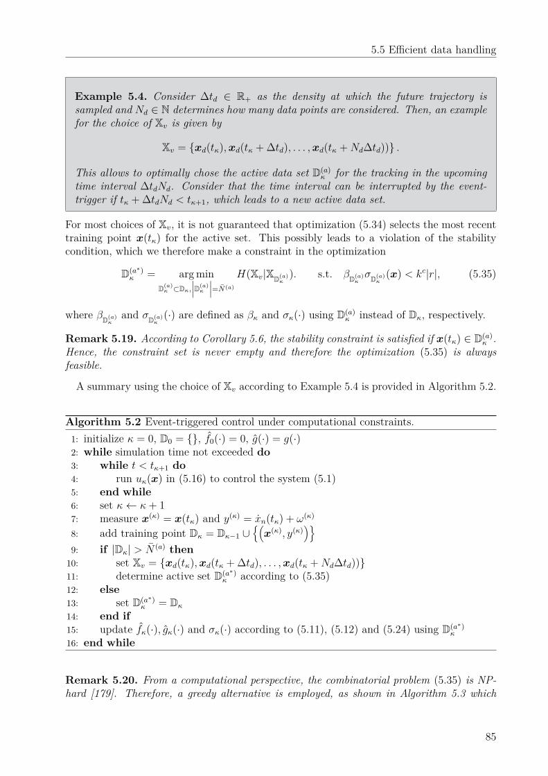
5.5 Efficient data handling
Example 5.4. Consider ∆td ∈ R+ as the density at which the future trajectory issampled and Nd ∈ N determines how many data points are considered. Then, an examplefor the choice of Xv is given by
Xv = xd(tκ),xd(tκ + ∆td), . . . ,xd(tκ +Nd∆td)) .
This allows to optimally chose the active data set D(a)κ for the tracking in the upcoming
time interval ∆tdNd. Consider that the time interval can be interrupted by the event-trigger if tκ + ∆tdNd < tκ+1, which leads to a new active data set.
For most choices of Xv, it is not guaranteed that optimization (5.34) selects the most recenttraining point x(tκ) for the active set. This possibly leads to a violation of the stabilitycondition, which we therefore make a constraint in the optimization
D(a∗)κ = arg min
D(a)κ ⊂Dκ,
∣∣∣D(a)κ
∣∣∣=N(a)
H(Xv|XD(a)κ
). s.t. βD(a)κσD(a)
κ(x) < kc|r|, (5.35)
where βD(a)κ
and σD(a)κ
(·) are defined as βκ and σκ(·) using D(a)κ instead of Dκ, respectively.
Remark 5.19. According to Corollary 5.6, the stability constraint is satisfied if x(tκ) ∈ D(a)κ .
Hence, the constraint set is never empty and therefore the optimization (5.35) is alwaysfeasible.
A summary using the choice of Xv according to Example 5.4 is provided in Algorithm 5.2.
Algorithm 5.2 Event-triggered control under computational constraints.1: initialize κ = 0, D0 = , f0(·) = 0, g(·) = g(·)2: while simulation time not exceeded do3: while t < tκ+1 do4: run uκ(x) in (5.16) to control the system (5.1)5: end while6: set κ← κ+ 17: measure x(κ) = x(tκ) and y(κ) = xn(tκ) + ω(κ)
8: add training point Dκ = Dκ−1 ∪(x(κ), y(κ)
)9: if |Dκ| > N (a) then
10: set Xv = xd(tκ),xd(tκ + ∆td), . . . ,xd(tκ +Nd∆td))11: determine active set D(a∗)
κ according to (5.35)12: else13: set D(a∗)
κ = Dκ
14: end if15: update fκ(·), gκ(·) and σκ(·) according to (5.11), (5.12) and (5.24) using D(a∗)
κ
16: end while
Remark 5.20. From a computational perspective, the combinatorial problem (5.35) is NP-hard [179]. Therefore, a greedy alternative is employed, as shown in Algorithm 5.3 which
85
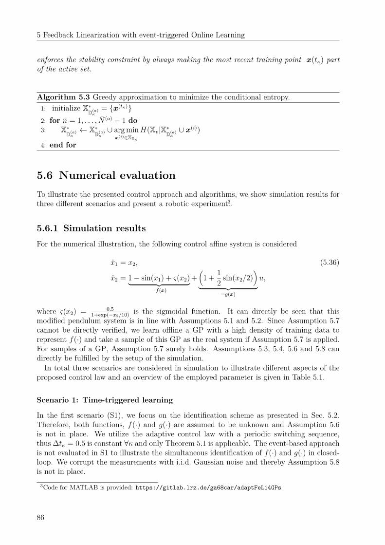
5 Feedback Linearization with event-triggered Online Learning
enforces the stability constraint by always making the most recent training point x(tκ) partof the active set.
Algorithm 5.3 Greedy approximation to minimize the conditional entropy.1: initialize X∗
D(a)κ
= x(tκ)2: for n = 1, . . . , N (a) − 1 do3: X∗
D(a)κ← X∗
D(a)κ∪ arg minx(i)∈XDκ
H(Xv|X∗D(a)κ∪ x(i))
4: end for
5.6 Numerical evaluationTo illustrate the presented control approach and algorithms, we show simulation results forthree different scenarios and present a robotic experiment.3.
5.6.1 Simulation resultsFor the numerical illustration, the following control affine system is considered
x1 = x2, (5.36)
x2 = 1− sin(x1) + ς(x2)︸ ︷︷ ︸=f(x)
+(
1 + 12 sin(x2/2)
)︸ ︷︷ ︸
=g(x)
u,
where ς(x2) = 0.51+exp(−x2/10) is the sigmoidal function. It can directly be seen that this
modified pendulum system is in line with Assumptions 5.1 and 5.2. Since Assumption 5.7cannot be directly verified, we learn offline a GP with a high density of training data torepresent f(·) and take a sample of this GP as the real system if Assumption 5.7 is applied.For samples of a GP, Assumption 5.7 surely holds. Assumptions 5.3, 5.4, 5.6 and 5.8 candirectly be fulfilled by the setup of the simulation.In total three scenarios are considered in simulation to illustrate different aspects of the
proposed control law and an overview of the employed parameter is given in Table 5.1.
Scenario 1: Time-triggered learning
In the first scenario (S1), we focus on the identification scheme as presented in Sec. 5.2.Therefore, both functions, f(·) and g(·) are assumed to be unknown and Assumption 5.6is not in place. We utilize the adaptive control law with a periodic switching sequence,thus ∆tκ = 0.5 is constant ∀κ and only Theorem 5.1 is applicable. The event-based approachis not evaluated in S1 to illustrate the simultaneous identification of f(·) and g(·) in closed-loop. We corrupt the measurements with i.i.d. Gaussian noise and thereby Assumption 5.8is not in place.
3Code for MATLAB is provided: https://gitlab.lrz.de/ga68car/adaptFeLi4GPs
86
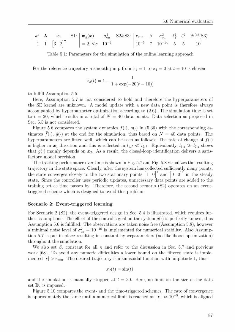
5.6 Numerical evaluation
kc λ x0 S1: mg(x) σ2on S2&S3: rmin β σ2
on `2f ζ2 N (a)(S3)
1 1[3 2
]ᵀ= 2, ∀x 10−6 10−5 7 10−14 5 5 10
Table 5.1: Parameters for the simulation of the online learning approach
For the reference trajectory a smooth jump from x1 = 1 to x1 = 0 at t = 10 is chosen
xd(t) = 1− 11 + exp(−20(t− 10))
to fulfill Assumption 5.5.Here, Assumption 5.7 is not considered to hold and therefore the hyperparameters of
the SE kernel are unknown. A model update with a new data point is therefore alwaysaccompanied by hyperparmeter optimization according to (2.6). The simulation time is setto t = 20, which results in a total of N = 40 data points. Data selection as proposed inSec. 5.5 is not considered.Figure 5.6 compares the system dynamics f(·), g(·) in (5.36) with the corresponding es-
timates f(·), g(·) at the end for the simulation, thus based on N = 40 data points. Thehyperparameters are fitted well, which can be seen as follows: The rate of change of f(·)is higher in x1 direction and this is reflected in l1,f l2,f . Equivalently, l1,g l2,g showsthat g(·) mainly depends on x2. As a result, the closed-loop identification delivers a satis-factory model precision.The tracking performance over time is shown in Fig. 5.7 and Fig. 5.8 visualizes the resulting
trajectory in the state space. Clearly, after the system has collected sufficiently many points,the state converges closely to the two stationary points
[1 0
]ᵀand
[0 0
]ᵀin the steady
state. Since the controller uses periodic updates, unnecessary data points are added to thetraining set as time passes by. Therefore, the second scenario (S2) operates on an event-triggered scheme which is designed to avoid this problem.
Scenario 2: Event-triggered learning
For Scenario 2 (S2), the event-triggered design in Sec. 5.4 is illustrated, which requires fur-ther assumptions: The effect of the control signal on the system g(·) is perfectly known, thusAssumption 5.6 is fulfilled. The observations are taken noise free (Assumption 5.8), howevera minimal noise level of σ2
on = 10−16 is implemented for numerical stability. Also Assump-tion 5.7 is put in place resulting in constant hyperparameters (no likelihood optimization)throughout the simulation.We also set βκ constant for all κ and refer to the discussion in Sec. 5.7 and previous
work [68]. To avoid any numeric difficulties a lower bound on the filtered state is imple-mented |r| > rmin. The desired trajectory is a sinusoidal function with amplitude 1, thus
xd(t) = sin(t),
and the simulation is manually stopped at t = 30. Here, no limit on the size of the dataset Dκ is imposed.Figure 5.10 compares the event- and the time-triggered schemes. The rate of convergence
is approximately the same until a numerical limit is reached at ‖e‖ ≈ 10−5, which is aligned
87
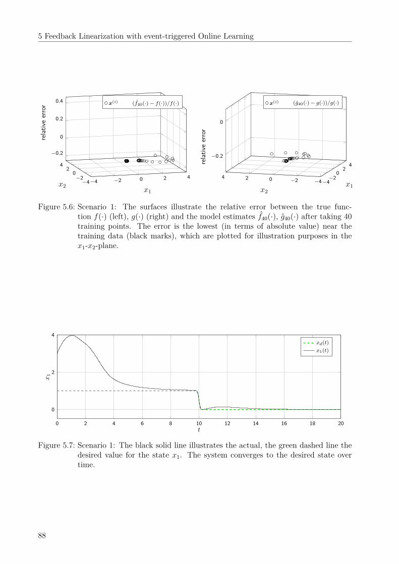
5 Feedback Linearization with event-triggered Online Learning
−4 −2 0 2 4−4
−20
24
−0.2
0
0.2
0.4
x1x2
relat
iveer
ror x(i) (f40(·) − f(·))/f(·)
−4−2
02
4
−4−2024
−0.2
0
x1x2
relat
iveer
ror
x(i) (g40(·) − g(·))/g(·)
Figure 5.6: Scenario 1: The surfaces illustrate the relative error between the true func-tion f(·) (left), g(·) (right) and the model estimates f40(·), g40(·) after taking 40training points. The error is the lowest (in terms of absolute value) near thetraining data (black marks), which are plotted for illustration purposes in thex1-x2-plane.
0 2 4 6 8 10 12 14 16 18 20
0
2
4
t
x1
xd(t)x1(t)
Figure 5.7: Scenario 1: The black solid line illustrates the actual, the green dashed line thedesired value for the state x1. The system converges to the desired state overtime.
88
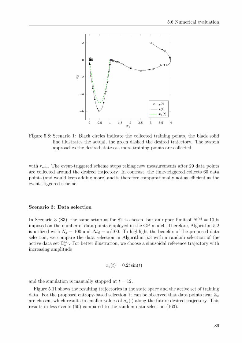
5.6 Numerical evaluation
0 0.5 1 1.5 2 2.5 3 3.5 4
−6
−4
−2
0
2
x1
x2
x(i)
x(t)xd(t)
Figure 5.8: Scenario 1: Black circles indicate the collected training points, the black solidline illustrates the actual, the green dashed the desired trajectory. The systemapproaches the desired states as more training points are collected.
with rmin. The event-triggered scheme stops taking new measurements after 29 data pointsare collected around the desired trajectory. In contrast, the time-triggered collects 60 datapoints (and would keep adding more) and is therefore computationally not as efficient as theevent-triggered scheme.
Scenario 3: Data selection
In Scenario 3 (S3), the same setup as for S2 is chosen, but an upper limit of N (a) = 10 isimposed on the number of data points employed in the GP model. Therefore, Algorithm 5.2is utilized with Nd = 100 and ∆td = π/100. To highlight the benefits of the proposed dataselection, we compare the data selection in Algorithm 5.3 with a random selection of theactive data set D(a)
κ . For better illustration, we choose a sinusoidal reference trajectory withincreasing amplitude
xd(t) = 0.2t sin(t)
and the simulation is manually stopped at t = 12.Figure 5.11 shows the resulting trajectories in the state space and the active set of training
data. For the proposed entropy-based selection, it can be observed that data points near Xv
are chosen, which results in smaller values of σκ(·) along the future desired trajectory. Thisresults in less events (60) compared to the random data selection (163).
89
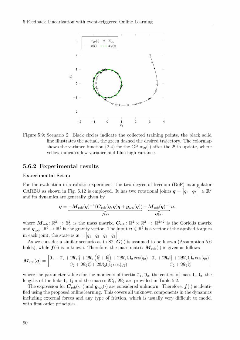
5 Feedback Linearization with event-triggered Online Learning
−2 −1 0 1 2 3 4
−2
−1
0
1
2
3
x1
x2
σ29(·) XDκ
x(t) xd(t)
Figure 5.9: Scenario 2: Black circles indicate the collected training points, the black solidline illustrates the actual, the green dashed the desired trajectory. The colormapshows the variance function (2.4) for the GP σ29(·) after the 29th update, whereyellow indicates low variance and blue high variance.
5.6.2 Experimental resultsExperimental Setup
For the evaluation in a robotic experiment, the two degree of freedom (DoF) manipulatorCARBO as shown in Fig. 5.12 is employed. It has two rotational joints q =
[q1 q2
]ᵀ ∈ R2
and its dynamics are generally given by
q = −M rob(q)−1 (Crob(q, q)q + grob(q))︸ ︷︷ ︸f(x)
+M rob(q)−1︸ ︷︷ ︸G(x)
u,
where M rob : R2 → S2+ is the mass matrix, Crob : R2 × R2 → R2×2 is the Coriolis matrix
and grob : R2 → R2 is the gravity vector. The input u ∈ R2 is a vector of the applied torquesin each joint, the state is x =
[q1 q2 q1 q2
]ᵀAs we consider a similar scenario as in S2, G(·) is assumed to be known (Assumption 5.6
holds), while f(·) is unknown. Therefore, the mass matrix M rob(·) is given as follows
M rob(q) =[I1 + I2 + M1l
21 + M2
(l21 + l22
)+ 2M2l1l2 cos(q2) I2 + M2l
22 + 2M2l1l2 cos(q2)
I2 + M2l22 + 2M2l1l2 cos(q2) I2 + M2l
22
]
where the parameter values for the moments of inertia I1, I2, the centers of mass l1, l2, thelengths of the links l1, l2 and the masses M1, M2 are provided in Table 5.2.The expression for Crob(·, ·) and grob(·) are considered unknown. Therefore, f(·) is identi-
fied using the proposed online learning. This covers all unknown components in the dynamicsincluding external forces and any type of friction, which is usually very difficult to modelwith first order principles.
90
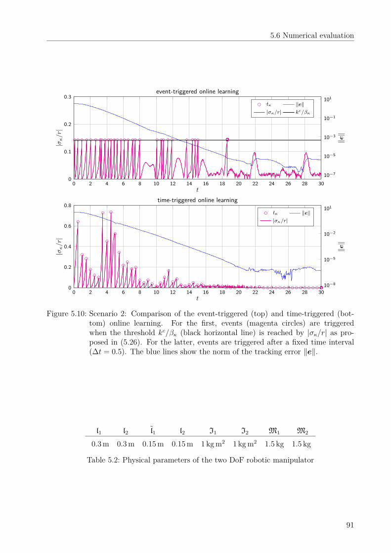
5.6 Numerical evaluation
0 2 4 6 8 10 12 14 16 18 20 22 24 26 28 300
0.1
0.2
0.3
t
|σκ/r|
event-triggered online learning
tκ ‖e‖|σκ/r| kc/βκ
10−7
10−5
10−3
10−1
101
‖e‖
0 2 4 6 8 10 12 14 16 18 20 22 24 26 28 300
0.2
0.4
0.6
0.8
t
|σκ/r
|
time-triggered online learning
tκ ‖e‖|σκ/r|
10−8
10−5
10−2
101
‖e‖
Figure 5.10: Scenario 2: Comparison of the event-triggered (top) and time-triggered (bot-tom) online learning. For the first, events (magenta circles) are triggeredwhen the threshold kc/βκ (black horizontal line) is reached by |σκ/r| as pro-posed in (5.26). For the latter, events are triggered after a fixed time interval(∆t = 0.5). The blue lines show the norm of the tracking error ‖e‖.
l1 l2 l1 l2 I1 I2 M1 M2
0.3 m 0.3 m 0.15 m 0.15 m 1 kg m2 1 kg m2 1.5 kg 1.5 kg
Table 5.2: Physical parameters of the two DoF robotic manipulator
91
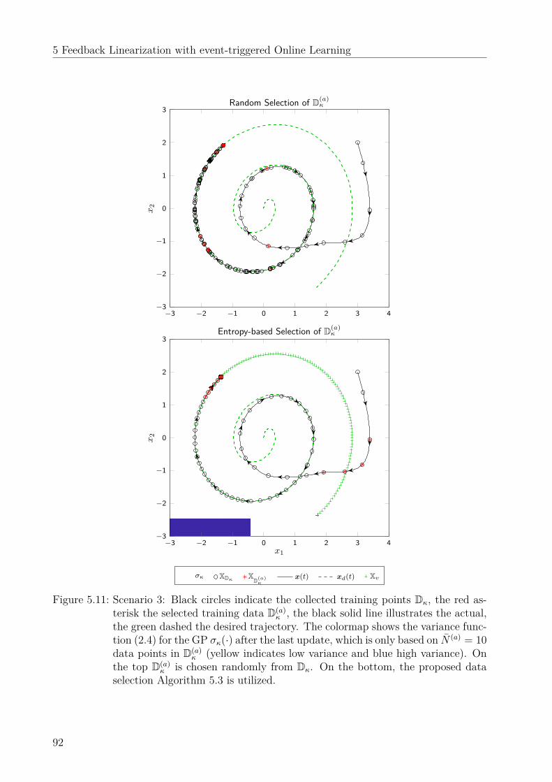
5 Feedback Linearization with event-triggered Online Learning
−3 −2 −1 0 1 2 3 4−3
−2
−1
0
1
2
3
x2
Random Selection of D(a)κ
−3 −2 −1 0 1 2 3 4−3
−2
−1
0
1
2
3
x1
x2
Entropy-based Selection of D(a)κ
σκ XDκ XD(a)κ
x(t) xd(t) Xv
Figure 5.11: Scenario 3: Black circles indicate the collected training points Dκ, the red as-terisk the selected training data D(a)
κ , the black solid line illustrates the actual,the green dashed the desired trajectory. The colormap shows the variance func-tion (2.4) for the GP σκ(·) after the last update, which is only based on N (a) = 10data points in D(a)
κ (yellow indicates low variance and blue high variance). Onthe top D(a)
κ is chosen randomly from Dκ. On the bottom, the proposed dataselection Algorithm 5.3 is utilized.
92
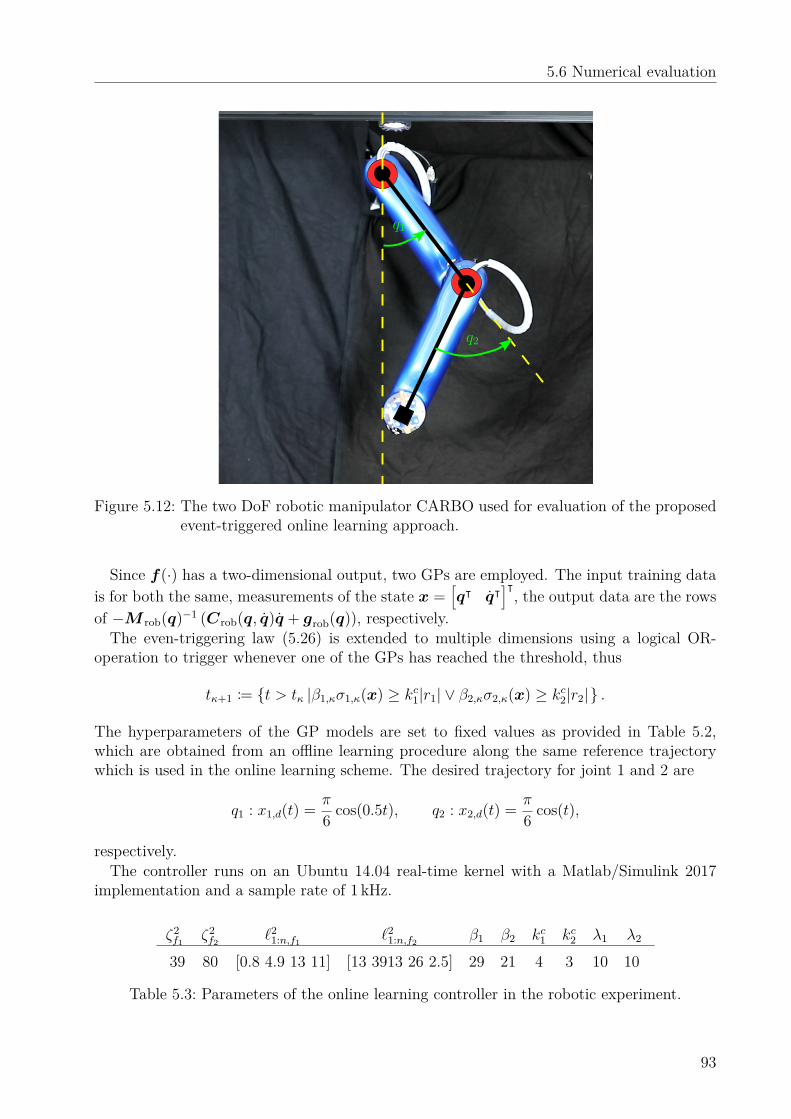
5.6 Numerical evaluation
q1
q2
Figure 5.12: The two DoF robotic manipulator CARBO used for evaluation of the proposedevent-triggered online learning approach.
Since f(·) has a two-dimensional output, two GPs are employed. The input training datais for both the same, measurements of the state x =
[qᵀ qᵀ
]ᵀ, the output data are the rows
of −M rob(q)−1 (Crob(q, q)q + grob(q)), respectively.The even-triggering law (5.26) is extended to multiple dimensions using a logical OR-
operation to trigger whenever one of the GPs has reached the threshold, thus
tκ+1 := t > tκ |β1,κσ1,κ(x) ≥ kc1|r1| ∨ β2,κσ2,κ(x) ≥ kc2|r2| .
The hyperparameters of the GP models are set to fixed values as provided in Table 5.2,which are obtained from an offline learning procedure along the same reference trajectorywhich is used in the online learning scheme. The desired trajectory for joint 1 and 2 are
q1 : x1,d(t) = π
6 cos(0.5t), q2 : x2,d(t) = π
6 cos(t),
respectively.The controller runs on an Ubuntu 14.04 real-time kernel with a Matlab/Simulink 2017
implementation and a sample rate of 1 kHz.
ζ2f1 ζ2
f2 `21:n,f1 `2
1:n,f2 β1 β2 kc1 kc2 λ1 λ2
39 80 [0.8 4.9 13 11] [13 3913 26 2.5] 29 21 4 3 10 10
Table 5.3: Parameters of the online learning controller in the robotic experiment.
93
5 Feedback Linearization with event-triggered Online Learning
Results
Similar to S2, we compare the proposed event-triggered online learning with a time-triggeredonline learning with ∆t = 0.5s and a model-free controller, where fκ(x) = 0, ∀x is usedin (5.4). The tracking error for both joints is shown in Figs. 5.13 and 5.14. The model-freecontroller (a PD controller with gains according to Table 5.3) shows no improvement overtime, while the event-triggered and the time-triggered control laws show decreasing trackingerrors.Figure 5.15 shows the accumulative number of model updates over time. While the pro-
posed event-triggered scheme adds most training points in the first period of the desiredtrajectory, the time-triggered scheme adds points at a constant rate. In the long run, thetime-triggered update law adds too many training data point because the real-time con-straint is violated for a data set with Nκ > 80. A problem which the event-triggered schemecircumvents because it only adds data points if required and is thereby more data-efficient.
5.7 DiscussionThe proposed approach safely controls unknown systems, even if no data points are initiallyavailable. This is a crucial novelty because many previous approaches do not discuss howtraining data can be collected without harming the system or its environment. The identifi-cation scheme relies on Bayesian principles which enables to incorporate prior knowledge ofthe closed-loop system structure into the model. It is very powerful since a very large classof functions f(·) and g(·) can be represented properly using the flexibility of a nonparametricmodel.The provided safety guarantees are based on the capability of the GP to measure its own
fidelity and thereby to bound the model error. This property, introduced in Theorem 2.1,requires Assumption 5.7, which is very crucial. Even though it is less restrictive than para-metric assumptions, it is still difficult to verify in practice. However, some assumptions arenecessary because a generalization outside of the training set would otherwise not be possi-ble [108]. Furthermore, the maximum mutual information γκ required in Theorem 2.1 is nottrivial to obtain. However, [104] provides for the most common kernels upper bounds on γκ.Furthermore, alternative bound, which do not require this value have already been pointedout [103].While this work mainly considers g(·), the effect of the control input on the dynamics, to be
known, it is also possible to learn it from data. An analysis of the resulting convergence prop-erties has been published recently [180] which allows to drop Assumption 5.6. While [180]only considers a static data set, we expect that an extension to the online event-triggeredcontroller is directly possible. Furthermore, this approach does not consider a limitation onthe control input. It can be shown, that u is bounded under the given assumptions, butpredefined limits cannot actively be imposed.The proposed event-triggered update law is highly data-efficient, since only necessary data
points are collected. The feedback linearizing controller only requires a locally precise model,which makes it sufficient to store only a single data point (compare Corollary 5.6). This is asignificant advantage over most existing approaches which require a globally precise modeland thereby a large data set.We are aware that two computational challenges remain open if the controller is applied
94
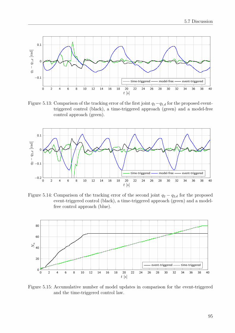
5.7 Discussion
0 2 4 6 8 10 12 14 16 18 20 22 24 26 28 30 32 34 36 38 40
−0.1
0
0.1
t [s]
q 1−
q 1,d
[rad]
time-triggered model-free event-triggered
Figure 5.13: Comparison of the tracking error of the first joint q1−q1,d for the proposed event-triggered control (black), a time-triggered approach (green) and a model-freecontrol approach (green).
0 2 4 6 8 10 12 14 16 18 20 22 24 26 28 30 32 34 36 38 40−0.2
−0.1
0
0.1
t [s]
q 2−
q 2,d
[rad]
time-triggered model-free event-triggered
Figure 5.14: Comparison of the tracking error of the second joint q2 − q2,d for the proposedevent-triggered control (black), a time-triggered approach (green) and a model-free control approach (blue).
0 2 4 6 8 10 12 14 16 18 20 22 24 26 28 30 32 34 36 38 400
20
40
60
80
t [s]
Nκ
event-triggered time-triggered
Figure 5.15: Accumulative number of model updates in comparison for the event-triggeredand the time-triggered control law.
95
5 Feedback Linearization with event-triggered Online Learning
over a long time scale. First, the current algorithm requires a growing (and unbounded)amount of memory since data is never deleted. However, the presented data selection schemehas already demonstrated, how data can safely be ignored by the controller. In fact, con-sidering the constraints (5.35), all non-active data could be deleted safely (maintaining theprovided convergence guarantees) leading to a O(1) memory usage. Also the number ofactive data points can be chosen very small (as low as N (a) = 1) leading to minimal datastorage requirements. Nevertheless, it should be considered that there is a trade-off betweenthe number of stored / active data points (memory) and the frequency of the events, whichare computationally quite expensive.Second, the selection of the active data set adds an additional computational burden and
the question whether it is beneficial requires a closer consideration: The greedy approxima-tion proposed in Algorithm 5.3 requires O
(NN (a)
)steps, while the model update (including
the matrix inversion) takes (with a rank-1 update) O(N (a)2) or O (N2) with or without data
selection, respectively. Thus, for N N (a) the selection can be expected to speed up themodel update step. But, even more important, the computation of the control law (GPposterior mean) requires O
(N (a)
)or O (N) steps and the detection of events (GP posterior
variance) takes O(N (a)2) or O (N2) steps with or without data selection, respectively. These
two operations are performed “continuously”, i.e. occur much more frequently than an eventand therefore the selection is expected to pay off for the overall computation time.In conclusion, this approach contributes to solve Challenges 2 and 4 because the control
law is safe from the first time instance, without requiring any knowledge of the system inadvance. In comparison, to previous methods like NN-based controllers in [181], it quantifiesthe ultimate bound for the tracking error and in comparison to [84] asymptotically stabilizesthe system. Key to this innovation is the event-triggered design of the control low whichallows safe exploration of unknown areas while safely following a reference trajectory.
5.8 SummaryThis chapter proposes a closed-loop nonparametric identification scheme for control-affinesystems. It takes advantage of compound kernels to transfer knowledge about the system’sstructure into the model. Based on feedback linearization, the control law achieves globaluniform ultimate boundedness of the tracking error for model updates at arbitrary timeinstances.Furthermore, an event-triggered online learning scheme is proposed, which collects new
training data only when necessary to ensure stability. This results in asymptotic stabilityguarantees for noise free measurements. To keep the control law computationally tractablethis chapter presents an optimal selection of the most informative data points with respectto the future desired trajectory.The proposed algorithms are illustrated in multiple simulation scenarios and evaluated in
a robotic experiment.
96
Further Work 6
In addition to the contributions presented in Chapters 3 to 5, the author has publishedfurther work in the intersection of machine learning and control. This chapter summarizesthese contributions very briefly. For more details, we refer to the respective publications.
6.1 Dynamic uncertainty-based leader-follower controlHumans cooperate very successfully in a variety of tasks, even if knowledge about the taskis distributed asymmetrically among cooperation partners [182]. A common cooperationparadigm for asymmetric knowledge distribution is the so-called leader-follower scheme.Here, the well-informed partner adopts a leading role, while the less knowledgeable part-ner assumes a following role. Leader-follower schemes are well established in control [183],but the roles are rarely adapted dynamically (during task execution) and often not assignedbased on knowledge.Therefore, the work in [102] proposes a knowledge-based cooperation scheme using GPs.
When an agent has high training data density in the current phase of the task, its GPposterior variance is low and it has high confidence about the task. As a result, it takes overa leading role, by being less cooperative and rather tracking its desired trajectory. When onlylittle training data is currently available, the GP posterior variance increases and the agentfocuses on cooperation (here, it strives to maintain the formation), rather than following itsuncertain estimate of a desired trajectory. The comparison to a constant cooperation schemeis shown in Fig. 6.1.
6.2 Uncertainty modeling in programming bydemonstration
The most appealing property of GPs is their representation of the fidelity of the model.However, most approaches ignore that the GP posterior variance function only representsthe proximity to training data and thereby models uncertainty due to missing data. However,there might also be uncertainty due to contradiction in the data or multi-modality, which isnot modeled by a GP.Particularly, in learning by demonstration in robotics, where multiple demonstrations of
the same task exist, the variability of the data carries crucial information about the taskitself. For example, in the manipulation of an object, a phase with low demonstrationvariability might indicate a narrow passage in the task space.
97
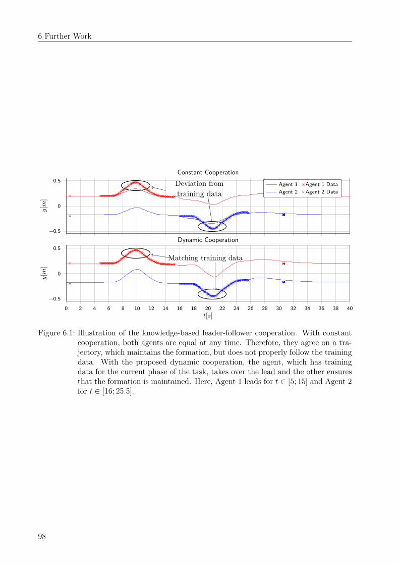
6 Further Work
−0.5
0
0.5 Deviation fromtraining data
y[m
]
Constant CooperationAgent 1 Agent 1 DataAgent 2 Agent 2 Data
0 2 4 6 8 10 12 14 16 18 20 22 24 26 28 30 32 34 36 38 40−0.5
0
0.5
Matching training data
t[s]
y[m
]
Dynamic Cooperation
Figure 6.1: Illustration of the knowledge-based leader-follower cooperation. With constantcooperation, both agents are equal at any time. Therefore, they agree on a tra-jectory, which maintains the formation, but does not properly follow the trainingdata. With the proposed dynamic cooperation, the agent, which has trainingdata for the current phase of the task, takes over the lead and the other ensuresthat the formation is maintained. Here, Agent 1 leads for t ∈ [5; 15] and Agent 2for t ∈ [16; 25.5].
98
6.3 Scenario-based optimal control
The work in [170] proposes a GP-based modeling technique by applying Wishart-processes(presented in [184]) to a learning by demonstration scenario. In the reproduction of the pre-sented motion, the stiffness of the robot is increased in phases with low variability in thetraining data and decreased where variability is high. Thereby, the controller is only aggres-sive when necessary and increases the safety in human-robot interaction. A visualization isprovided in Fig. 6.2.
6.3 Scenario-based optimal controlDrawing (and storing) a sample from a GP is practically impossible because it is an infinitedimensional object [106]. This might be the reason why the scenario view on GPs is theleast utilized among the presented interpretations in Sec. 2.3. Nevertheless, model predictivecontrol schemes do not need to sample an entire function, but only a finite number of functionvalues.This insight enables the combination of a scenario-based optimal control approach and GP
models in [107]. By sampling trajectories over a finite time horizon from a GP dynamicalmodel, the variety of possible outcomes is properly represented. The work uses a differentialdynamic programming approach to solve the optimal control problem. Based on the resultfrom robust convex optimization, performance guarantees are derived. A visualization ofthis scenario-based approach is provided in Fig. 6.3.
6.4 Uncertainty-aware path trackingMany programming by demonstration tasks require the replication or generalization of apresented path. In a large fraction of the literature, the desired motion is modeled as adynamical system, due to its robustness to perturbation and real-time capability. Mostworks also provide guarantees for convergence to the desired final point, see e.g., dynamicmovement primitives (DMP) [185] or stable estimator of dynamical systems (SEDS) [123].However, all previous works ignore the uncertainty, which comes with sparse training data.
In contrast, the work in [186] develops an uncertainty-based path tracking, which activelymakes use of the capability of a GPSSM to quantify its uncertainty due to missing data. Theapproach actively strives into regions with more demonstration data and thus higher modelcertainty, which allows to reproduce human-demonstrated motions with higher precisionthan competitive state-of-the-art methods.It is designed for goal-directed tasks, where it is essential to impose stability constraints on
the model representing the human motion to make sure it reaches the correct final position.To guarantee this stability of the resulting trajectories, the presented approach uses a non-parametric GP-based Lyapunov function, which is visualized in Fig. 6.4.
6.5 Learning a stable state-dependent coefficient formWhile most other contributions in this thesis focus on GPs, the work in [187] presents amore general framework to learn stable stochastic dynamical systems. More specifically,it considers the state-dependent coefficient form, which can represent arbitrary continuous
99
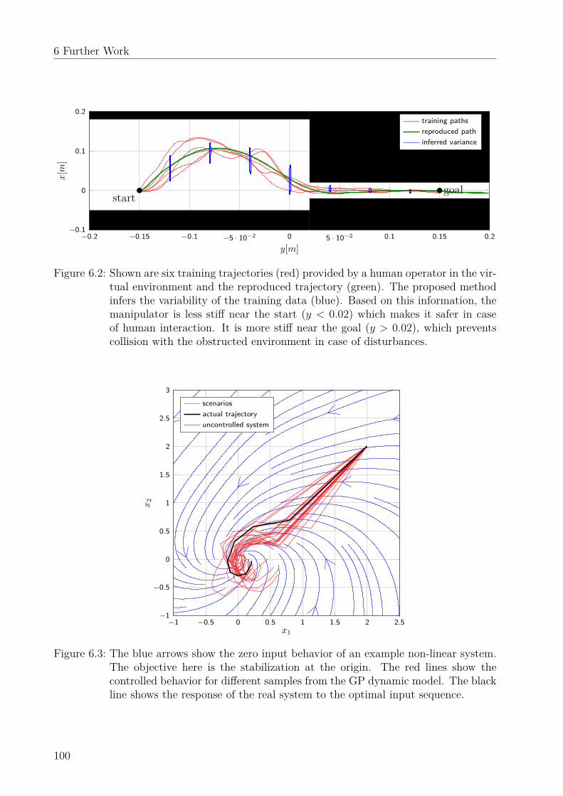
6 Further Work
−0.2 −0.15 −0.1 −5 · 10−2 0 5 · 10−2 0.1 0.15 0.2−0.1
0
0.1
0.2
startgoal
y[m]
x[m
]
training pathsreproduced pathinferred variance
Figure 6.2: Shown are six training trajectories (red) provided by a human operator in the vir-tual environment and the reproduced trajectory (green). The proposed methodinfers the variability of the training data (blue). Based on this information, themanipulator is less stiff near the start (y < 0.02) which makes it safer in caseof human interaction. It is more stiff near the goal (y > 0.02), which preventscollision with the obstructed environment in case of disturbances.
−1 −0.5 0 0.5 1 1.5 2 2.5−1
−0.5
0
0.5
1
1.5
2
2.5
3
x1
x2
scenariosactual trajectoryuncontrolled system
Figure 6.3: The blue arrows show the zero input behavior of an example non-linear system.The objective here is the stabilization at the origin. The red lines show thecontrolled behavior for different samples from the GP dynamic model. The blackline shows the response of the real system to the optimal input sequence.
100
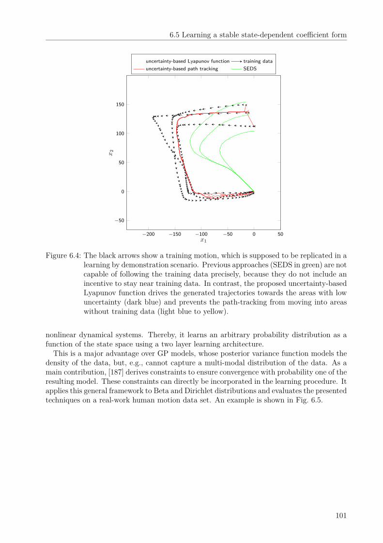
6.5 Learning a stable state-dependent coefficient form
−200 −150 −100 −50 0 50
−50
0
50
100
150
x1
x2
uncertainty-based Lyapunov function training datauncertainty-based path tracking SEDS
Figure 6.4: The black arrows show a training motion, which is supposed to be replicated in alearning by demonstration scenario. Previous approaches (SEDS in green) are notcapable of following the training data precisely, because they do not include anincentive to stay near training data. In contrast, the proposed uncertainty-basedLyapunov function drives the generated trajectories towards the areas with lowuncertainty (dark blue) and prevents the path-tracking from moving into areaswithout training data (light blue to yellow).
nonlinear dynamical systems. Thereby, it learns an arbitrary probability distribution as afunction of the state space using a two layer learning architecture.This is a major advantage over GP models, whose posterior variance function models the
density of the data, but, e.g., cannot capture a multi-modal distribution of the data. As amain contribution, [187] derives constraints to ensure convergence with probability one of theresulting model. These constraints can directly be incorporated in the learning procedure. Itapplies this general framework to Beta and Dirichlet distributions and evaluates the presentedtechniques on a real-work human motion data set. An example is shown in Fig. 6.5.
101
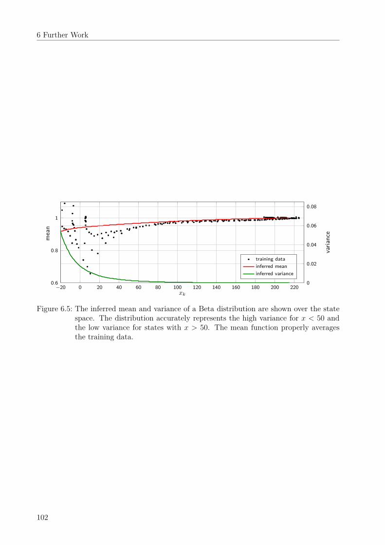
6 Further Work
−20 0 20 40 60 80 100 120 140 160 180 200 2200.6
0.8
1
xk
mea
n
training datainferred meaninferred variance
0
0.02
0.04
0.06
0.08
varia
nce
Figure 6.5: The inferred mean and variance of a Beta distribution are shown over the statespace. The distribution accurately represents the high variance for x < 50 andthe low variance for states with x > 50. The mean function properly averagesthe training data.
102
Conclusion 7
The application of data-driven models in control significantly progressed over the past years.More and more publications focus on formal guarantees of model-based control laws andtake the present uncertainties due to imperfect modeling into consideration. This progressimproves the reliability of learning-based control and supports its application in safety-criticaldomains, e.g., autonomous driving or physical human robot interaction.This thesis focuses on Gaussian processes (GPs) as data-driven models and contributes
novel concepts for system identification and the design of control laws which are summarizedin the following.
Summary of contributionsAfter the introduction, we present in Chapter 2 a structured literature review on GPs incontrol and classify different interpretations of GPs used in existing works. Then, for theidentification of dynamical systems, we propose a framework to impose consistent conver-gence behavior of the real unknown system and the nonparametric model. In a physicalcontext, this ensures that the model also follows the principle of energy dissipation. Theframework learns the convergence behavior from data and ensures this is mimicked by theGaussian process state space model. We show that this approach under certain conditionsnever performs worse than a GP model without stabilization. In contrast to previous work,we include the uncertainty due to sparse training data in the model and derive how manydata points are needed to guarantee asymptotic stability.To take advantage of data-driven models, which include an estimate of the model fidelity,
we propose a control law which actively avoids areas in the state space where the modeluncertainty is high. The analysis shows that it is optimal, with respect to the probability ofconvergence, to steer the system along a trajectory near the training data where the modelprecision is high. This behavior is intuitive but has not been shown formally before.If a training data set is not available, safe exploration of an unknown system is crucial.
Therefore, we propose an online learning feedback linearizing control law, which is stable fromthe start and continuously improves the model over time. This event-triggered control schemetakes new measurements only if necessary and is thereby highly data-efficient. Compared toother online methods, it only operates on a local model making it unnecessary to store a largedata set for a globally valid model. We show asymptotic stability of the resulting closed-loop switching system and propose an information-theoretic selection of data to reduce thecomputational complexity.All results are supported by rigorous mathematical proofs along with numerical evalua-
tions, showing that the proposed concepts are significant contributions to make data-drivenmodels for control applicable in safety-critical domains.
103
7 Conclusion
Implications
We take this chance to revisit the challenges imposed for learning-based control in Sec. 1.1.
Challenge 1 Making a model logically and physically consistent with the real systemrequires to consider various aspects. In Chapter 3 this thesis focuses on the dissipation ofenergy. Learning not only the dynamics but also the convergence behavior from data allowsto combine the flexibility of nonparametric models with consistent stability properties of thetrue system and the model. Further physical or logical verifications of the model are notstudied.
Challenge 2 The question on formal guarantees and the required assumptions is addressedby the two proposed control laws, in an offline setting in Chapter 4 and an online settingin Chapter 5. Both show that despite the present uncertainties, asymptotic stability canbe achieved in both cases. Two assumptions are necessary to draw this conclusion. First,the volatility of the dynamics must be restricted (here a bound on the reproducing kernelHilbert space norm), which corresponds to a smooth dynamical system. Second, knowledgeabout the effect of the input on the state is required. While the first assumption is inevitable,according to the no-free-lunch theorems [108], the second originates from the chosen feedbacklinearizing control design.
Challenge 3 The existing control approaches which avoid uncertain areas and favor well-known areas, known as risk-sensitive control [129], are largely missing an analysis of stability.In Chapter 4 this work presents a novel controller which maximizes the probability forstability under a given power constraint and shows the desired risk-aware behavior for data-driven models.
Challenge 4 Systems for which initially no training data exists must be explored safelythrough an online closed-loop identification. Since the control law proposed in Chapter 5requires only a locally precise model, the closed-loop stability can be guaranteed from thestart and thereby allows safe exploration of unknown systems. Focusing on data efficiency,we develop an event-triggered update scheme which only adds training points if necessarydue to a high model uncertainty. It thereby answers the question which data points shouldbe collected. By proposing a safe forgetting strategy, which uses the information gain ascriteria, we also address the question which data points should be kept in case of dataprocessing or storage constraints.
Future directions
Although this thesis presents novel techniques to learning-based control and thereby makesprogress towards the safe application in various tasks, many problems remain unsolved. Wewould like to point out these open research questions, which we suggest to study in thefuture.
104
Safe online learning
The simultaneous identification and control of an unknown system is, within this thesis, onlydiscussed in Chapter 5 and is also underrepresented in the literature. However, this is one ofthe most urgent difficulties in the field. The assumption that an initial data set is availableis hard to justify because there might be no safe method to obtain the data. Therefore,algorithms are required which start with no data points initially and safely control thesystem while exploring the state space. The idea of life-long learning, where data pointsare constantly added during operation, is important for constant improvement, however,solutions must be found to an infinitely increasing data set.
Computational and data efficiency
Gaussian processes are a computationally very heavy tool, which becomes intractable in mostreal-time applications for more than 104 data points. While there are many good reasonsto choose GPs as a dynamical model (among others its very good generalization for smalldata sets), a solution must be found for complex systems with high dimensional state space.Since these require large data sets for precise control, the computational tractability and thedata efficiency must be a focus of future work. The contribution in Sec. 5.5.1 is only a stepin this direction.
Systems with unknown state spaces
An assumption, which was not explicitly stated here, is that the state space of the systemis known. However, if the fundamental (physical) relations of a complex system are notunderstood, it might not just be impossible to derive the dynamics but also difficult todefine the state space. An example which is often mentioned for the application of data-driven control is soft-robotics [188]. However, flexible structures typically require an analysisusing finite element methods, which is only an approximation to an infinite dimensional statespace. Therefore, future work must transfer the presented ideas to an input-output view ofa dynamical system, which comes with many more challenges regarding observability andcontrollability of learned systems.
State and input constraints
The notion of safety in this thesis only considers the asymptotic behavior of the system,i.e. the derived bounds (e.g. on the tracking error) are not satisfied at all times, but areonly ensured as time approaches infinity. One idea to resolve this difficulty is to analyze therate of convergence using Lyapunov-based techniques, which guarantees a certain trackingprecision for a given (finite) time interval. However, there exist various control approaches,e.g., MPC, control barrier functions and invariance control, which directly allow to imposestate or input constraints in the design. Combining those methods with data-driven modelsand performing a rigorous analysis of the closed-loop behavior will be of great value for manysafety-critical applications.
105

7 Conclusion
Formal guarantees with alternative regression models
The work in this thesis is focused on GPs because it allows to bound the model error undermild assumptions and thereby allows to prove formal stability results for the proposed controllaws. However, GPs also have disadvantages (e.g., a high computational complexity), whichis the reason why most publications in the field of machine learning focus on alternativeapproaches, such as neural network. Transferring the presented techniques and proofs toother supervised learning techniques would make data-driven control applicable in morecomplex tasks and empower learning-based control to operate large scale systems.
106

Notation
Acronyms & Abbreviationsa.s. almost surely
CLF control Lyapunov function
DoF degree of freedom
DMP dynamic movement primitives
GP Gaussian process
GPSSM Gaussian process state space model
GUUB globally uniformly ultimately bounded
GAS globally asymptotically stable
HJB Hamilton-Jacobi-Bellman
i.i.d. independent and identically distributed
ILC iterative learning control
LQR linear quadratic regulator
MPC model predictive control
MRAC model reference adaptive control
NN neural network
RKHS reproducing kernel Hilbert space
RL reinforcement learning
SE squared exponential
SEDS stable estimator of dynamical systems
SOS sum of squares
UAV unmanned aerial vehicle
107

Notation
UGAS uniformly globally asymptotically stable
UB ultimately bounded
UUV unmanned underwate vehicle
WSAQF weighted sum of asymmetric quadratic functions
Conventions & Operators|·| absolute value of a real number or cardinality of a set
IN ∈ RN×N identity matrix
E[·] expected value of a random variable
V[·] variance of a random variable
·(i) i-th training point
·ᵀ transpose of a vector or matrix
‖·‖ Euclidean norm of a vector (if not state differently)
diag(·, ·, · · · ) arranges the elements on the diagonal of a diagonal matrix
‖·‖k reproducing kernel Hilbert space norm of a function
〈·, ·〉 inner product of a vector space
· ∼ N (·, ·) random variable follows a Gaussian distribution with mean and variance
· ∼ GP(·, ·) function is distributed according to a Gaussian process with mean andvariance function
1 : N integer indices from 1 to N , thus 1, 2, . . . ,N
x(1:N) concatenation of x1 to xN , thus [x1 · · · xN ]ᵀ
f(x(1:N)
)concatenation of function evaluations, thus
[f(x(1)
)· · · f
(x(N)
)]ᵀO(·) big O notation to describe limiting behavior of functions
P · probability of an event
p (·) probability density function
det(·) determinate of a matrix
log(·) natural logarithm of a positive scalar
rank(·) rank of a matrix
108

Notation
trace(·) trace of a matrix
x ∈ (a; b) open interval, thus a < x < b
x ∈ [a; b] closed interval, thus a ≤ x ≤ b
∇x · Nabla operator, gradient of a scalar function
∇xᵀ · Nabla operator, gradient transpose of a scalar fucntion
%(·), %(·) minimal and maximal singular value of a matrix, respectively
$(·), $(·) minimal and maximal eigenvalue value of a matrix, respectively
0 vector/matrix of zeros of proper dimensions
Sets & SpacesB,Bι,Bι ⊆ X hyperball (with radius ι, ι)
Bσon ⊆ X hyperball whose radius depends on the observation noise σon
Bκ ⊆ X hyperball at κ-th time step
D, Dκ set of training data (after κ model updates)
D(a)κ ,D(a∗)
κ (optimal) set of active training data at the κ-th time step
Dadd set of additional training data
L2 the space of square-integrable functions
N set of positive integers
R, R+,R+,0 set of real / positive real / non-negative real numbers
Sn+ ⊂ Rn×n set of symmetric positive definite n× n matrices
Snε$ ⊆ Sn+ set of symmetric n× n matrices, with all eigenvalues larger than ε$
U ⊆ Rnu set of control inputs
X ⊆ Rn state or input space, refer to definition
Xi∗ ⊆ X region of attraction of the i∗-th equilibrium point
Xi∗ ⊆ Xi∗ region around the i∗-th equilibrium point, refer to definition
Xd ⊂ X manifold of states of the future desired trajectory
Xa ⊂ X active input training points
Xv ⊂ X state of interest
109
Notation
Functionsα1,α2 : R+,0 → R+,0 class K functions, i.e. strictly increasing and α(0) = 0
b : Rn+ → (0; 1) computes the reliability for given error bounds
β : (0; 1)→ R+ computes the constant β given a probability
cσ : X→ R cost function to plan optimal path
Crob : R2 × R2 → R2×2 Coriolis matrix of a two DoF robotic manipulator
∆fκ, ∆f : X→ R+,0 model error (in the κ-th time step)
f : X→ R general scalar function, refer to definition
f : X→ Rm general vector field, refer to definition
f : X→ X stabilized GPSSM to estimate f(·)
f , fκ : X→ R approximation to the function f(·) (at time step κ)
f : X→ Rm approximation to the function f(·), refer to definition
fGP : X→ R Gaussian process estimate for f(·)
fBS : X× S+ → X× S+ dynamics in the belief-space interpretation
fsum, fprod : X→ R function, which is a sum / product of two functions
fa, fb, fh : X→ R functions, which are samples from a GP
grob : R2 → R2 gravity vector of a two DoF robotic manipulator
g : X→ R scaling of the input for a single input control affine system
G : X→ Rn×n scaling of the input for a control affine system
g, gκ : X→ R approximation to the function g(·) (at time step κ)
gκ : X→ R ratio of g(·) to gκ(·)
g : R→ R+ penalty function for fitting Lyapunov functions to data
g : R+ → R+ penalty function in the positive domain for fitting Lyapunovfunctions to data
h : X→ R scalar function in general, refer to definition
H : Xm → R+ entropy of m jointly distributed random variables
k, ka, kb, kh : X× X→ R kernel functions of a GP
kprod : X× X→ R kernel function for product of a GP and a known function
110

Notation
kSE : X× X→ R squared exponential kernel
kfg, kf , kg : X× X→ R kernel function for identification of control affine systems
k,ka,kb,kh,kg,kf: X→ RN covariances between a test input x and the trainingdata x(1:N)
M rob : R2 → S2+ mass matrix of a two DoF robotic manipulator
mon : X→ Rnpoly vector of monomials
M , N : R→ R auxiliarily functions, refer to definition
m,ma,mb : X→ R prior mean function of a GP
µ : X→ R posterior mean function of a GP in general
µf ,µg : X→ R posterior mean function of a GP to model functions f(·)and g(·), respectively
µ : X→ Rm posterior mean function of m GPs concatenated as vector
ppoly : X→ R polynomial of degree dpoly
p : R→ R+ probability density function, refer to definition
σ : X→ R posterior standard deviation of a GP
σ : X→ Rm posterior standard deviation of m GPs concatenated asvector
σ2 : X→ R posterior variance function of a GP
Σ : X→ Rm×m posterior variance function of m GPs concatenated asdiagonal matrix
σ2 : X→ Rm posterior variance function of m GPs concatenated as vector
σ2D2 : X→ R posterior variance of a GP for a dataset with two points
ς : R→ (−0.5; 0.5)) shifted sigmoid function
V : X→ R+,0 general Lyapunov candidate, refer to defintion
Vσ : X→ R+,0 uncertainty-aware Lyapunov function
Vclf : X→ R+,0 generic control Lyapunov function
Vval : X→ R+,0 value function for an optimal control problem
Vθ,V i∗θi∗
: X→ R+,0 parameterized Lyapunov function learned from data
VSq : X→ R+,0 quadratic Lyapunov function
Vsq : X→ R+,0 isotropic quadratic Lyapunov function
111

Notation
VSOS : X→ R+,0 sum of squares Lyapunov function
VWSAQF : X→ R+,0 weighted sum of asymmetric squares Lyapunov function
W0 : [9 exp(91);∞)→ [91;∞) principle branch of the Lambert W function
W91 : [9 exp(91); 0)→ [9∞; 91) lower branch of the Lambert W function
V ,V : R+,0 → R+,0 auxiliarily functions to decompose a Lyapunov function
x : [0 S]→ X path parameterized by the arclength s ∈ [0;S]
Z,Z : R+ × X→ R auxiliarily functions to analyze the posterior variance
Z ′,Z ′ : R+ → R auxiliarily functions to analyze the posterior variance
Constants & Variablesβ ∈ R+, β ∈ Rm
+ constants linking the model error to the variance of a GP
bB ∈ R+ desired size of the ultimate bound
Bf ∈ R bound for the reproducing kernel Hilbert space norm of f(·)
c1, c2 ∈ R auxiliarily constants, refer to definition
c1, c3 ∈ Rn constants to bound terms of a Lyapunov function
C2,C3 ∈ Sn+ constants to bound terms of a Lyapunov function
c1,φκ , c2,φκ ∈ R+,0 constants defined for notational convenience
dpoly ∈ N degree of a monomial
δ ∈ (0; 1) probability that the model error of a GP violates a certain bound
Ecor ∈ R+,0 correction effort, refer to definition
e ∈ Rn tracking error
ε ∈ R+ arbitrarily small constant
εfd ∈ R+ constant to compute numerical gradients using finite differences
ε$ ∈ R+ lower bound for eigenvalues of positive definite matrices
εV ∈ R+ constant to resolve strict inequality constraints
γ ∈ R+ maximum mutual information
gconst ∈ R+ gravity constant
H ∈ RN×N diagonal matrix with h(x(i)
), i = 1, . . . ,N on its diagonal
112
Notation
i ∈ 1, . . . ,N index (mainly used for training points)
i∗ ∈ 1, . . . ,N∗ index for equilibria
Ii∗ ⊆ 1, 2, . . . ,N indices of data points within the i∗-region of attraction
i ∈ 0, 1 indicator variable for WSAQF
I1, I2 ∈ R+ moment of inertia of a two DoF robotic manipulator
j ∈ 1, . . . ,n index (mainly used for dimensions of the state space)
κ ∈ N0 time index for time-discrete event-triggered systems
kc ∈ R+ controller gain
K,Ka,Kb,Kh ∈RN×N covariance matrix of training data
Kf ,Kg ∈ RN×N covariance matrix of training data for kf (·, ·) / kg(·, ·)
Ksum,Kprod ∈ RN×N covariance matrix of training data, refer to definition
Kon ∈ RN×N covariance matrix of training data including observation noise
Kfg ∈ RN×N covariance matrix of training data for the compoundkernel kfg(·, ·) including observation noise
Kol,cl ∈ RNol×N covariance matrix of training data for open- and closed-loopmeasurements
Kol,ol ∈ RNol×Nol covariance matrix of training data for open-loop measurements
`2 ∈ R+ lengthscale of a SE kernel
`2j,f , `2
j,g ∈ R+ lengthscale of SE kernel kf (·, ·), kg(·, ·), respectively
`2 ∈ R+ smallest lengthscale of (multiple) SE kernel(s)
%G∈ R+,0 smallest singular value of a matrix G
Lσ ∈ R+ Lipschitz constant of GP posterior standard deviation function
l ∈ 1, . . . ,L indexing variable in WSAQF
L ∈ N number of asymmetric squared functions in WSAQF
l1, l2 ∈ R+ length of links of two DoF robotic manipulator
l1, l2 ∈ R+ center of mass for each link of two DoF robotic manipulator
λ1, . . . ,λn−1 ∈ R coefficients of a linear filter
λ ∈ Rn−1 concatenation of coefficients of a linear filter
ηi∗ ∈ R+,0 measure how well a Lyapunov function fits data
113

Notation
M1,M2 ∈ R+ mass of each link of a two DoF robotic manipulator
µxκ+1 ∈ X mean of the next state in belief-space view
µ ∈ R+ upper bound for GP posterior mean function
n ∈ N dimensionality of an input or state space
N ∈ N number of training points
Nol ∈ N number of training points obtained from open-loop measurements
N (a)κ ∈ N number of training points in the active data set in the κ-th time
step
N (a) ∈ N budget (maximum number of training points in active data set)
Nd ∈ N number of points sampled from future desired trajectory
N∗ ∈ N number of equilibria
Ninit ∈ N number of different initial points
Nvio ∈ N number of trajectories violating the ultimate bound
Nadd ∈ N number of added data points
npoly ∈ N number of a monomials with a degree dpoly in n dimensions
ν ∈ R linear feedback control
ω ∈ R,ω ∈ Rn independent and identically distributed noise
ψ,ψfg hyperparameters of a Gaussian process / composite kernel kfg(·, ·)
φ ∈ R upper bound for triggering condition
P 0...L ∈ Sn+ coefficient matrices for the WSAQF
P ∈ Rn×n coefficient matrix for a quadratic function
Q ∈ Rn×n coefficient matrix for sum of squares function
q1, q2 ∈ R, q ∈ R2 joint angles of a two DoF robot in radiants
rtr ∈ R+ radius around a training point
ρ ∈ R filtered tracking error
r ∈ R filtered state
rmin ∈ R+ lower bound for the absolute value of r
ra, ra ∈ R+,0 distances in the state space, refer to definition
114

Notation
Υ1, . . . , Υn ∈ N exponents of monomials
ι, ι ∈ R+ radius of a ball or utlimate bound
σon ∈ R+,0 standard deviation of the observation noise
σ2on ∈ R+,0 variance of the observation noise
ζ2 ∈ R+,0 signal variance of a SE kernel
ζ2f , ζ2
g ∈ R+,0 signal variance of SE kernel kf (·, ·), kg(·, ·), respectively
ζ2 ∈ R+,0 maximal signal variance of mutiple SE kernels
σ2 ∈ R+ upper bound for GP posterior variance
σ ∈ R+ upper bound for GP posterior standard deviation
σ2xκ+1 ∈ R+ variance of the state in belief-space view
s ∈ C complex variable in a characteristic polynomial
s ∈ R paramterization of a path
S ∈ R upper limit for paramterization of a path
θ ∈ Θ,θi∗ ∈ Θi∗ parameter vector for Lyapunov function Vθ(·),V i∗θi∗
(·)
Θ, Θi∗ ⊆ Rnθ possible parameter set with dimension nθ
tκ ∈ R+ current time instance
tκ+1 ∈ R+ next time instance
∆t, ∆tκ ∈ R+ time interval (in the κ-th step)
∆td ∈ R+ time interval at which the future desired trajectory is sampled
∆t ∈ R+ lower bound for the inter-event time
τ ∈ R+ auxiliarily variable, refer to definition
υ ∈ (0; 1) reliability (probability that a system is stable)
u ∈ R, u ∈ Rnu control input, refer to definition
umax ∈ R+ maximum control power
U ∈ RN×N diagonal matrix with control input at training points
x ∈ X state of a system / input to a function
xκ,xκ ∈ X current state of a time discrete system
xκ+1,xκ+1 ∈ X next state of a time discrete system
115

Notation
xg ∈ X goal state to which a system converges
xkn ∈ X state at which the function value is known
x∗, xi∗ ∈ X estimate of the (i∗-)equilibrium point
x∗,xi∗ ∈ X the (i∗-th) equilibrium point
x(a),x(a) ∈ X specific points in the state space, refer to definition
xd ∈ X desired trajectory
xWSAQF1 , . . . ,xWSAQF
L ∈X centers in the weighted sum of asymmetric quadratic functions
y ∈ R,y ∈ Rn noisy measurement of the output of a function
ykn ∈ R known function value at xkn
ysum ∈ R noisy measurements of the sum of two functions
yprod ∈ R noisy measurements of the product of two functions
yol ∈ R noisy open loop measurements
z ∈ R auxiliarily variable
116
List of Figures
2.1 Deterministic and robust interpretation of a GP model. . . . . . . . . . . . . 112.2 Belief-space interpretation of a GP model. . . . . . . . . . . . . . . . . . . . 122.3 Stochastic and scenario interpretation of a GP model. . . . . . . . . . . . . . 132.4 Illustration of Lemma 2.1 . . . . . . . . . . . . . . . . . . . . . . . . . . . . 17
3.1 Illustration of a training dataset . . . . . . . . . . . . . . . . . . . . . . . . . 213.2 Illustration for a system with multiple equilibria . . . . . . . . . . . . . . . . 223.3 Overview of the proposed data-driven stabilization of GPSSMs . . . . . . . . 233.4 Illustration for the optimization-based stabilization . . . . . . . . . . . . . . 273.5 Visualization for the proof of Theorem 3.2 . . . . . . . . . . . . . . . . . . . 303.6 Norm of trajectories of Example 3.2 on stochastic stability . . . . . . . . . . 313.7 Longterm simulation of Example 3.2 on stochastic stability . . . . . . . . . . 313.8 Illustration of the proof of Theorem 3.3 . . . . . . . . . . . . . . . . . . . . . 363.9 GP posterior variance for two data points . . . . . . . . . . . . . . . . . . . 363.10 Optimization-based learning of Lyapunov functions from data . . . . . . . . 383.11 Identification of an unknown equilibrium from data . . . . . . . . . . . . . . 433.12 Illustration of the area error employed as quality measure . . . . . . . . . . . 443.13 Stochastic simulation of a GPSSM . . . . . . . . . . . . . . . . . . . . . . . . 45
4.1 Illustration of the proof for Theorem 4.1 . . . . . . . . . . . . . . . . . . . . 534.2 Illustration for Example 4.1 . . . . . . . . . . . . . . . . . . . . . . . . . . . 534.3 Visualization of the trained GPSSM . . . . . . . . . . . . . . . . . . . . . . . 604.4 Simulated trajectories for the uncertainty-aware control approach . . . . . . 60
5.1 Overview of the proposed online learning control law . . . . . . . . . . . . . 655.2 Example for inferring the sum of functions with structured kernels . . . . . . 685.3 Example for inferring the product of functions with structured kernels . . . . 705.4 Example for inferring the sum of functions with additional data . . . . . . . 735.5 Overview of the event-triggered feedback linearizing control structure . . . . 745.6 Comparing the model estimates with the true system . . . . . . . . . . . . . 885.7 Tracking error for time-triggered updates of the data set . . . . . . . . . . . 885.8 Trajectory for time-triggered updates of the data set . . . . . . . . . . . . . 895.9 Trajectory for event-triggered updates of the data set . . . . . . . . . . . . . 905.10 Comparing event-triggered and time-triggered events . . . . . . . . . . . . . 915.11 Trajectory for event-triggered updates with selected data . . . . . . . . . . . 925.12 The two DoF robotic manipulator CARBO . . . . . . . . . . . . . . . . . . . 935.13 Comparing tracking error in robotic experiment (first joint) . . . . . . . . . . 955.14 Comparing tracking error in robotic experiment (second joint) . . . . . . . . 95
117

List of Figures
5.15 Events triggered in the robotic experiment . . . . . . . . . . . . . . . . . . . 95
6.1 Illustration of the knowledge-based leader-follower cooperation . . . . . . . . 986.2 Illustration of uncertainty modeling in programming by demonstration . . . 1006.3 Illustration of a scenario-based optimal control approach for GPs . . . . . . . 1006.4 Illustration of the uncertainty-aware path tracking . . . . . . . . . . . . . . . 1016.5 Illustration of learning a stable system with Beta distributions . . . . . . . . 102
118

List of Tables
3.1 Performance and properties of different Lyapunov functions . . . . . . . . . . 46
5.1 Parameters for the simulation of the online learning approach . . . . . . . . 875.2 Physical parameters of the two DoF robotic manipulator . . . . . . . . . . . 915.3 Parameters of the online learning controller in the robotic experiment. . . . . 93
119


List of Algorithms
3.1 Stable identification and prediction for GPSSMs . . . . . . . . . . . . . . . . 41
5.1 Adaptive feedback linearization control . . . . . . . . . . . . . . . . . . . . . 745.2 Event-triggered control under computational constraints. . . . . . . . . . . . 855.3 Greedy approximation to minimize entropy . . . . . . . . . . . . . . . . . . . 86
121

Bibliography
[1] D. Silver, J. Schrittwieser, K. Simonyan, I. Antonoglou, A. Huang, A. Guez, T. Hu-bert, L. Baker, M. Lai, A. Bolton, et al., “Mastering the game of go without humanknowledge”, Nature, vol. 550, no. 7676, pp. 354–359, 2017.
[2] C. E. Rasmussen and C. K. I. Williams, Gaussian Processes for Machine Learning.Cambridge, MA, USA: MIT Press, 2006.
[3] A. Krizhevsky, I. Sutskever, and G. E. Hinton, “Imagenet classification with deep con-volutional neural networks”, in Advances in Neural Information Processing Systems(NeurIPS), Curran Associates, Inc., 2012, pp. 1097–1105.
[4] N. Du, Y. Wang, N. He, J. Sun, and L. Song, “Time-sensitive recommendation fromrecurrent user activities”, in Advances in Neural Information Processing Systems(NeurIPS), Curran Associates, Inc., 2015, pp. 3492–3500.
[5] P. Ponte and R. G. Melko, “Kernel methods for interpretable machine learning oforder parameters”, Physical Review B, vol. 96, no. 20, p. 205 146, 20 2017.
[6] D. H. Wolpert and W. G. Macready, “No free lunch theorems for optimization”, IEEETransactions on Evolutionary Computation, vol. 1, no. 1, pp. 67–82, 1997.
[7] J. Umlauft, A. Lederer, and S. Hirche, “Learning stable Gaussian process state spacemodels”, in American Control Conference (ACC), IEEE, 2017, pp. 1499–1504.
[8] J. Umlauft and S. Hirche, “Learning stochastically stable Gaussian process state-spacemodels”, IFAC Journal of Systems and Control, vol. 12, p. 100 079, 2020.
[9] J. Umlauft, L. Pöhler, and S. Hirche, “An uncertainty-based control Lyapunov ap-proach for control-affine systems modeled by Gaussian process”, IEEE Control Sys-tems Letters, vol. 2, no. 3, pp. 483–488, 2018.
[10] J. Umlauft, T. Beckers, M. Kimmel, and S. Hirche, “Feedback linearization usingGaussian processes”, in Conference on Decision and Control (CDC), IEEE, 2017,pp. 5249–5255.
[11] J. Umlauft and S. Hirche, “Feedback linearization based on Gaussian processes withevent-triggered online learning”, IEEE Transactions on Automatic Control (TAC),pp. 1–16, 2020.
[12] J. Umlauft, T. Beckers, A. Capone, A. Lederer, and S. Hirche, “Smart forgetting forsafe online learning with Gaussian processes”, in Learning for Dynamics and Control(L4DC), ser. Proceedings of Machine Learning Research, vol. 120, The Cloud: PMLR,2020, pp. 160–169.
123
Bibliography
[13] T. Beckers, J. Umlauft, and S. Hirche, “Mean square prediction error of misspecifiedGaussian process models”, in Conference on Decision and Control (CDC), IEEE,2018, pp. 1162–1167.
[14] M. Liu, G. Chowdhary, B. Castra da Silva, S. Y. Liu, and J. P. How, “Gaussianprocesses for learning and control: A tutorial with examples”, IEEE Control SystemsMagazine, vol. 38, no. 5, pp. 53–86, 2018.
[15] J. Kocijan, Modelling and Control of Dynamic Systems Using Gaussian Process Mod-els. Springer, 2016.
[16] L. Ljung, System Identification. NJ, USA: Prentice Hall PTR, 1998.[17] K. Narendra and K. Parthasarathy, “Adaptive identification and control of dynamical
systems using neural networks”, in Conference on Decision and Control (CDC), vol. 2,IEEE, 1989, pp. 1737–1738.
[18] M. M. Polycarpou and P. A. Ioannou, Identification and control of nonlinear systemsusing neural network models: Design and stability analysis. University of SouthernCalif., 1991.
[19] P. M. Nørgård, O. Ravn, N. K. Poulsen, and L. K. Hansen, Neural Networks forModelling and Control of Dynamic Systems - A Practitioner’s Handbook. London:Springer, 2000.
[20] J. Kocijan, B. Banko, B. Likar, A. Girard, R. Murray-Smith, and C. E. Rasmussen,“A case based comparison of identification with neural network and Gaussian pro-cess models.”, in International Conference on Intelligent Control Systems and SignalProcessing (ICONS), Max-Planck-Gesellschaft, vol. 1, 2003, pp. 137–142.
[21] J. Kocijan, A. Girard, B. Banko, and R. Murray-Smith, “Dynamic systems identifica-tion with Gaussian processes”, Mathematical and Computer Modelling of DynamicalSystems, vol. 11, no. 4, pp. 411–424, 2005.
[22] J. M. Maciejowski, Predictive control: with constraints. Prentice Hall, 2002.[23] A. Girard, C. E. Rasmussen, J. Quinonero-Candela, and R. Murray-Smith, “Multiple-
step ahead prediction for non linear dynamic systems–a Gaussian process treatmentwith propagation of the uncertainty”, Advances in Neural Information ProcessingSystems (NeurIPS), vol. 15, pp. 529–536, 2002.
[24] J. Kocijan, “Dynamic GP models: An overview and recent developments”, in Inter-national Conference on Applied Mathematics, Simulation, Modelling (ASM), 2012,pp. 38–43.
[25] J. Kocijan, “Control algorithms based on Gaussian process models: A state-of-the-artsurvey”, in Special International Conference on Complex Systems: Synergy of Control,Communications and Computing (COSY), 2011, pp. 69–80.
[26] T. Beckers and S. Hirche, “Stability of Gaussian process state space models”, inEuropean Control Conference (ECC), 2016, pp. 2275–2281.
[27] ——, “Equilibrium distributions and stability analysis of Gaussian process state spacemodels”, in Conference on Decision and Control (CDC), IEEE, 2016, pp. 6355–6361.
124
Bibliography
[28] M. Kuss and C. E. Rasmussen, “Gaussian processes in reinforcement learning”, inAdvances in Neural Information Processing Systems (NeurIPS), Curran Associates,Inc., 2004, pp. 751–758.
[29] D. Sbarbaro and R. Murray-Smith, “Self-tuning control of non-linear systems us-ing Gaussian process prior models”, in Switching and Learning in Feedback Systems:European Summer School on Multi-Agent Control, Maynooth, Ireland, September 8-10, 2003, Revised Lectures and Selected Papers. Berlin, Heidelberg: Springer BerlinHeidelberg, 2005, pp. 140–157.
[30] M. P. Deisenroth, C. E. Rasmussen, and J. Peters, “Model-based reinforcement learn-ing with continuous states and actions”, in European Symposium on Artificial NeuralNetworks (ESANN), 2008.
[31] J. Hall, C. E. Rasmussen, and J. Maciejowski, “Reinforcement learning with referencetracking control in continuous state spaces”, in Conference on Decision and Control(CDC), IEEE, 2011, pp. 6019–6024.
[32] M. P. Deisenroth and C. E. Rasmussen, “PILCO: A model-based and data-efficient ap-proach to policy search”, in International Conference on Machine Learning (ICML),2011, pp. 465–472.
[33] M. P. Deisenroth, Efficient reinforcement learning using Gaussian processes. KITScientific Publishing, 2010, vol. 9.
[34] J. Hall, C. E. Rasmussen, and J. Maciejowski, “Modelling and control of nonlinearsystems using Gaussian processes with partial model information”, in Conference onDecision and Control (CDC), IEEE, 2012, pp. 5266–5271.
[35] M. P. Deisenroth, C. E. Rasmussen, and D. Fox, “Learning to control a low-costmanipulator using data-efficient reinforcement learning”, in Robotics: Science andSystems VII. MITP, 2012, ch. 8, pp. 57–64.
[36] M. P. Deisenroth, D. Fox, and C. E. Rasmussen, “Gaussian processes for data-efficientlearning in robotics and control”, IEEE Transactions on Pattern Analysis and Ma-chine Intelligence, vol. 37, no. 2, pp. 408–423, 2015.
[37] M. P. Deisenroth, G. Neumann, J. Peters, et al., “A survey on policy search forrobotics”, Foundations and Trends in Robotics, vol. 2, no. 1–2, pp. 1–142, 2013.
[38] J. Vinogradska, B. Bischoff, J. Achterhold, T. Koller, and J. Peters, “Numericalquadrature for probabilistic policy search”, Transactions on Pattern Analysis andMachine Intelligence, vol. 42, pp. 164–175, 1 2018.
[39] J. Vinogradska, B. Bischoff, D. Nguyen-Tuong, H. Schmidt, A. Romer, and J. Pe-ters, “Stability of controllers for Gaussian process forward models”, in InternationalConference on Machine Learning (ICML), JMLR, NY, USA, 2016, pp. 545–554.
[40] J. Vinogradska, “Gaussian processes in reinforcement learning: Stability analysis andefficient value propagation”, PhD thesis, Technical University of Darmstadt, 2018.
[41] B. Bethke and J. P. How, “Approximate dynamic programming using bellman resid-ual elimination and Gaussian process regression”, in American Control Conference(ACC), IEEE, 2009, pp. 745–750.
125
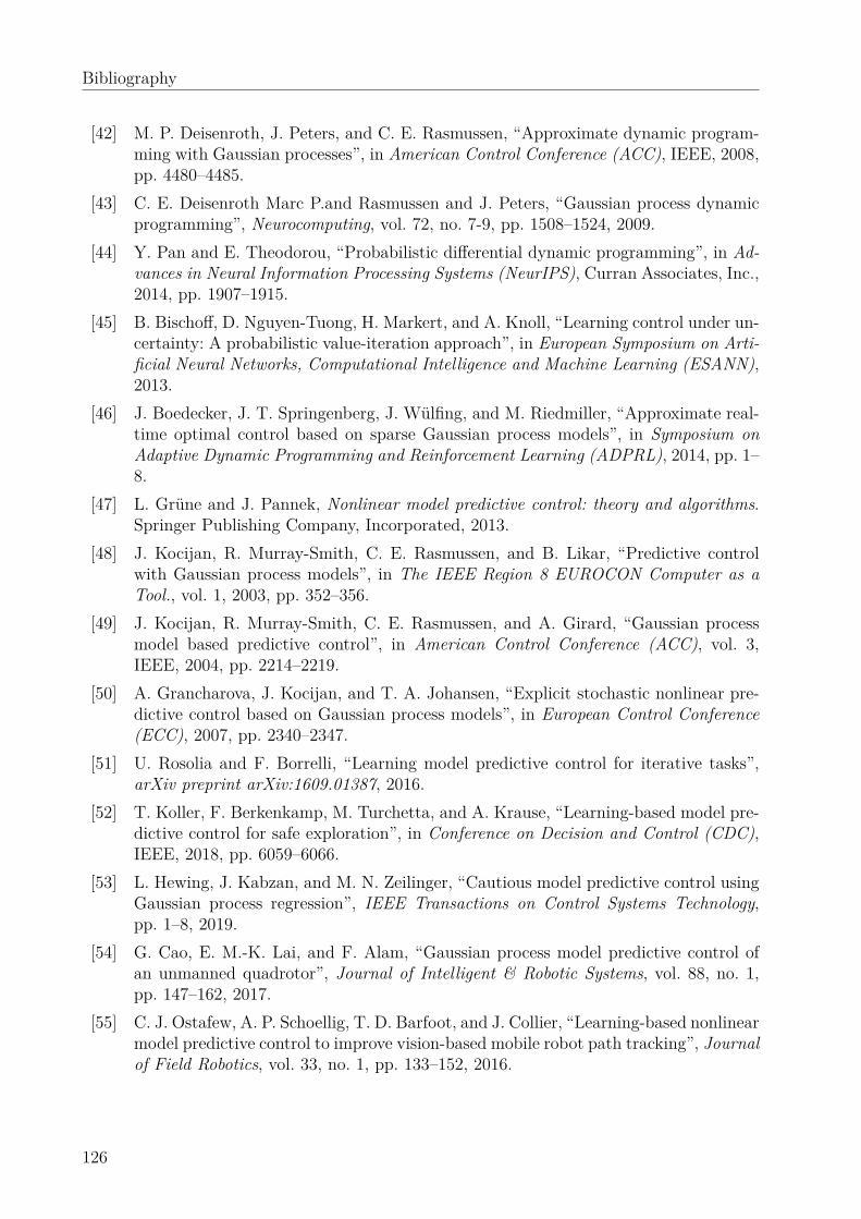
Bibliography
[42] M. P. Deisenroth, J. Peters, and C. E. Rasmussen, “Approximate dynamic program-ming with Gaussian processes”, in American Control Conference (ACC), IEEE, 2008,pp. 4480–4485.
[43] C. E. Deisenroth Marc P.and Rasmussen and J. Peters, “Gaussian process dynamicprogramming”, Neurocomputing, vol. 72, no. 7-9, pp. 1508–1524, 2009.
[44] Y. Pan and E. Theodorou, “Probabilistic differential dynamic programming”, in Ad-vances in Neural Information Processing Systems (NeurIPS), Curran Associates, Inc.,2014, pp. 1907–1915.
[45] B. Bischoff, D. Nguyen-Tuong, H. Markert, and A. Knoll, “Learning control under un-certainty: A probabilistic value-iteration approach”, in European Symposium on Arti-ficial Neural Networks, Computational Intelligence and Machine Learning (ESANN),2013.
[46] J. Boedecker, J. T. Springenberg, J. Wülfing, and M. Riedmiller, “Approximate real-time optimal control based on sparse Gaussian process models”, in Symposium onAdaptive Dynamic Programming and Reinforcement Learning (ADPRL), 2014, pp. 1–8.
[47] L. Grüne and J. Pannek, Nonlinear model predictive control: theory and algorithms.Springer Publishing Company, Incorporated, 2013.
[48] J. Kocijan, R. Murray-Smith, C. E. Rasmussen, and B. Likar, “Predictive controlwith Gaussian process models”, in The IEEE Region 8 EUROCON Computer as aTool., vol. 1, 2003, pp. 352–356.
[49] J. Kocijan, R. Murray-Smith, C. E. Rasmussen, and A. Girard, “Gaussian processmodel based predictive control”, in American Control Conference (ACC), vol. 3,IEEE, 2004, pp. 2214–2219.
[50] A. Grancharova, J. Kocijan, and T. A. Johansen, “Explicit stochastic nonlinear pre-dictive control based on Gaussian process models”, in European Control Conference(ECC), 2007, pp. 2340–2347.
[51] U. Rosolia and F. Borrelli, “Learning model predictive control for iterative tasks”,arXiv preprint arXiv:1609.01387, 2016.
[52] T. Koller, F. Berkenkamp, M. Turchetta, and A. Krause, “Learning-based model pre-dictive control for safe exploration”, in Conference on Decision and Control (CDC),IEEE, 2018, pp. 6059–6066.
[53] L. Hewing, J. Kabzan, and M. N. Zeilinger, “Cautious model predictive control usingGaussian process regression”, IEEE Transactions on Control Systems Technology,pp. 1–8, 2019.
[54] G. Cao, E. M.-K. Lai, and F. Alam, “Gaussian process model predictive control ofan unmanned quadrotor”, Journal of Intelligent & Robotic Systems, vol. 88, no. 1,pp. 147–162, 2017.
[55] C. J. Ostafew, A. P. Schoellig, T. D. Barfoot, and J. Collier, “Learning-based nonlinearmodel predictive control to improve vision-based mobile robot path tracking”, Journalof Field Robotics, vol. 33, no. 1, pp. 133–152, 2016.
126
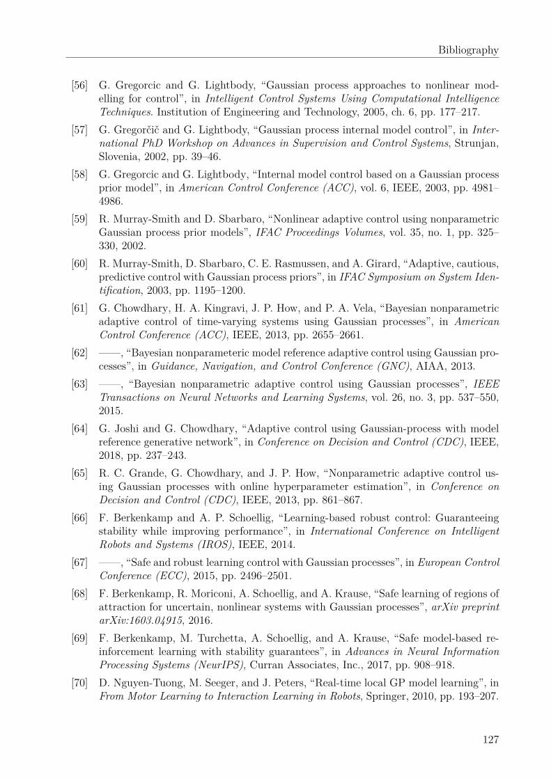
Bibliography
[56] G. Gregorcic and G. Lightbody, “Gaussian process approaches to nonlinear mod-elling for control”, in Intelligent Control Systems Using Computational IntelligenceTechniques. Institution of Engineering and Technology, 2005, ch. 6, pp. 177–217.
[57] G. Gregorčič and G. Lightbody, “Gaussian process internal model control”, in Inter-national PhD Workshop on Advances in Supervision and Control Systems, Strunjan,Slovenia, 2002, pp. 39–46.
[58] G. Gregorcic and G. Lightbody, “Internal model control based on a Gaussian processprior model”, in American Control Conference (ACC), vol. 6, IEEE, 2003, pp. 4981–4986.
[59] R. Murray-Smith and D. Sbarbaro, “Nonlinear adaptive control using nonparametricGaussian process prior models”, IFAC Proceedings Volumes, vol. 35, no. 1, pp. 325–330, 2002.
[60] R. Murray-Smith, D. Sbarbaro, C. E. Rasmussen, and A. Girard, “Adaptive, cautious,predictive control with Gaussian process priors”, in IFAC Symposium on System Iden-tification, 2003, pp. 1195–1200.
[61] G. Chowdhary, H. A. Kingravi, J. P. How, and P. A. Vela, “Bayesian nonparametricadaptive control of time-varying systems using Gaussian processes”, in AmericanControl Conference (ACC), IEEE, 2013, pp. 2655–2661.
[62] ——, “Bayesian nonparameteric model reference adaptive control using Gaussian pro-cesses”, in Guidance, Navigation, and Control Conference (GNC), AIAA, 2013.
[63] ——, “Bayesian nonparametric adaptive control using Gaussian processes”, IEEETransactions on Neural Networks and Learning Systems, vol. 26, no. 3, pp. 537–550,2015.
[64] G. Joshi and G. Chowdhary, “Adaptive control using Gaussian-process with modelreference generative network”, in Conference on Decision and Control (CDC), IEEE,2018, pp. 237–243.
[65] R. C. Grande, G. Chowdhary, and J. P. How, “Nonparametric adaptive control us-ing Gaussian processes with online hyperparameter estimation”, in Conference onDecision and Control (CDC), IEEE, 2013, pp. 861–867.
[66] F. Berkenkamp and A. P. Schoellig, “Learning-based robust control: Guaranteeingstability while improving performance”, in International Conference on IntelligentRobots and Systems (IROS), IEEE, 2014.
[67] ——, “Safe and robust learning control with Gaussian processes”, in European ControlConference (ECC), 2015, pp. 2496–2501.
[68] F. Berkenkamp, R. Moriconi, A. Schoellig, and A. Krause, “Safe learning of regions ofattraction for uncertain, nonlinear systems with Gaussian processes”, arXiv preprintarXiv:1603.04915, 2016.
[69] F. Berkenkamp, M. Turchetta, A. Schoellig, and A. Krause, “Safe model-based re-inforcement learning with stability guarantees”, in Advances in Neural InformationProcessing Systems (NeurIPS), Curran Associates, Inc., 2017, pp. 908–918.
[70] D. Nguyen-Tuong, M. Seeger, and J. Peters, “Real-time local GP model learning”, inFrom Motor Learning to Interaction Learning in Robots, Springer, 2010, pp. 193–207.
127
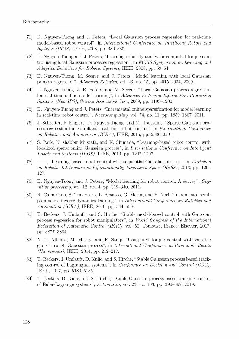
Bibliography
[71] D. Nguyen-Tuong and J. Peters, “Local Gaussian process regression for real-timemodel-based robot control”, in International Conference on Intelligent Robots andSystems (IROS), IEEE, 2008, pp. 380–385.
[72] D. Nguyen-Tuong and J. Peters, “Learning robot dynamics for computed torque con-trol using local Gaussian processes regression”, in ECSIS Symposium on Learning andAdaptive Behaviors for Robotic Systems, IEEE, 2008, pp. 59–64.
[73] D. Nguyen-Tuong, M. Seeger, and J. Peters, “Model learning with local Gaussianprocess regression”, Advanced Robotics, vol. 23, no. 15, pp. 2015–2034, 2009.
[74] D. Nguyen-Tuong, J. R. Peters, and M. Seeger, “Local Gaussian process regressionfor real time online model learning”, in Advances in Neural Information ProcessingSystems (NeurIPS), Curran Associates, Inc., 2009, pp. 1193–1200.
[75] D. Nguyen-Tuong and J. Peters, “Incremental online sparsification for model learningin real-time robot control”, Neurocomputing, vol. 74, no. 11, pp. 1859–1867, 2011.
[76] J. Schreiter, P. Englert, D. Nguyen-Tuong, and M. Toussaint, “Sparse Gaussian pro-cess regression for compliant, real-time robot control”, in International Conferenceon Robotics and Automation (ICRA), IEEE, 2015, pp. 2586–2591.
[77] S. Park, K. shabbir Mustafa, and K. Shimada, “Learning-based robot control withlocalized sparse online Gaussian process”, in International Conference on IntelligentRobots and Systems (IROS), IEEE, 2013, pp. 1202–1207.
[78] ——, “Learning based robot control with sequential Gaussian process”, in Workshopon Robotic Intelligence in Informationally Structured Space (RiiSS), 2013, pp. 120–127.
[79] D. Nguyen-Tuong and J. Peters, “Model learning for robot control: A survey”, Cog-nitive processing, vol. 12, no. 4, pp. 319–340, 2011.
[80] R. Camoriano, S. Traversaro, L. Rosasco, G. Metta, and F. Nori, “Incremental semi-parametric inverse dynamics learning”, in International Conference on Robotics andAutomation (ICRA), IEEE, 2016, pp. 544–550.
[81] T. Beckers, J. Umlauft, and S. Hirche, “Stable model-based control with Gaussianprocess regression for robot manipulators”, in World Congress of the InternationalFederation of Automatic Control (IFAC), vol. 50, Toulouse, France: Elsevier, 2017,pp. 3877–3884.
[82] N. T. Alberto, M. Mistry, and F. Stulp, “Computed torque control with variablegains through Gaussian process”, in International Conference on Humanoid Robots(Humanoids), IEEE, 2014, pp. 212–217.
[83] T. Beckers, J. Umlauft, D. Kulic, and S. Hirche, “Stable Gaussian process based track-ing control of Lagrangian systems”, in Conference on Decision and Control (CDC),IEEE, 2017, pp. 5180–5185.
[84] T. Beckers, D. Kulić, and S. Hirche, “Stable Gaussian process based tracking controlof Euler-Lagrange systems”, Automatica, vol. 23, no. 103, pp. 390–397, 2019.
128
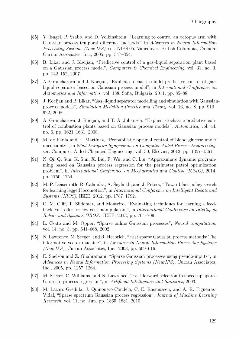
Bibliography
[85] Y. Engel, P. Szabo, and D. Volkinshtein, “Learning to control an octopus arm withGaussian process temporal difference methods”, in Advances in Neural InformationProcessing Systems (NeurIPS), ser. NIPS’05, Vancouver, British Columbia, Canada:Curran Associates, Inc., 2005, pp. 347–354.
[86] B. Likar and J. Kocijan, “Predictive control of a gas–liquid separation plant basedon a Gaussian process model”, Computers & Chemical Engineering, vol. 31, no. 3,pp. 142–152, 2007.
[87] A. Grancharova and J. Kocijan, “Explicit stochastic model predictive control of gas–liquid separator based on Gaussian process model”, in International Conference onAutomatics and Informatics, vol. 188, Sofia, Bulgaria, 2011, pp. 85–88.
[88] J. Kocijan and B. Likar, “Gas–liquid separator modelling and simulation with Gaussian-process models”, Simulation Modelling Practice and Theory, vol. 16, no. 8, pp. 910–922, 2008.
[89] A. Grancharova, J. Kocijan, and T. A. Johansen, “Explicit stochastic predictive con-trol of combustion plants based on Gaussian process models”, Automatica, vol. 44,no. 6, pp. 1621–1631, 2008.
[90] M. de Paula and E. Martinez, “Probabilistic optimal control of blood glucose underuncertainty”, in 22nd European Symposium on Computer Aided Process Engineering,ser. Computer Aided Chemical Engineering, vol. 30, Elsevier, 2012, pp. 1357–1361.
[91] N. Qi, Q. Sun, K. Sun, X. Liu, F. Wu, and C. Liu, “Approximate dynamic program-ming based on Gaussian process regression for the perimeter patrol optimizationproblem”, in International Conference on Mechatronics and Control (ICMC), 2014,pp. 1750–1754.
[92] M. P. Deisenroth, R. Calandra, A. Seyfarth, and J. Peters, “Toward fast policy searchfor learning legged locomotion”, in International Conference on Intelligent Robots andSystems (IROS), IEEE, 2012, pp. 1787–1792.
[93] O. M. Cliff, T. Sildomar, and Monteiro, “Evaluating techniques for learning a feed-back controller for low-cost manipulators”, in International Conference on IntelligentRobots and Systems (IROS), IEEE, 2013, pp. 704–709.
[94] L. Csato and M. Opper, “Sparse online Gaussian processes”, Neural computation,vol. 14, no. 3, pp. 641–668, 2002.
[95] N. Lawrence, M. Seeger, and R. Herbrich, “Fast sparse Gaussian process methods: Theinformative vector machine”, in Advances in Neural Information Processing Systems(NeurIPS), Curran Associates, Inc., 2003, pp. 609–616.
[96] E. Snelson and Z. Ghahramani, “Sparse Gaussian processes using pseudo-inputs”, inAdvances in Neural Information Processing Systems (NeurIPS), Curran Associates,Inc., 2005, pp. 1257–1264.
[97] M. Seeger, C. Williams, and N. Lawrence, “Fast forward selection to speed up sparseGaussian process regression”, in Artificial Intelligence and Statistics, 2003.
[98] M. Lazaro-Gredilla, J. Quinonero-Candela, C. E. Rasmussen, and A. R. Figueiras-Vidal, “Sparse spectrum Gaussian process regression”, Journal of Machine LearningResearch, vol. 11, no. Jun, pp. 1865–1881, 2010.
129
Bibliography
[99] J. Quinonero-Candela and C. E. Rasmussen, “A unifying view of sparse approximateGaussian process regression”, The Journal of Machine Learning Research, vol. 6,pp. 1939–1959, 2005.
[100] E. Snelson and Z. Ghahramani, “Local and global sparse Gaussian process approxi-mations”, in International Conference on Artificial Intelligence and Statistics, 2007,pp. 524–531.
[101] S. Choi, K. Lee, and S. Oh, “Robust learning from demonstration using leveragedGaussian processes and sparse-constrained optimization”, in International Conferenceon Robotics and Automation (ICRA), IEEE, 2016.
[102] Y. Fanger, J. Umlauft, and S. Hirche, “Gaussian processes for dynamic movementprimitives with application in knowledge-based cooperation”, in International Con-ference on Intelligent Robots and Systems (IROS), IEEE, 2016, pp. 3913–3919.
[103] A. Lederer, J. Umlauft, and S. Hirche, “Uniform error bounds for Gaussian processregression with application to safe control”, in Advances in Neural Information Pro-cessing Systems (NeurIPS), Curran Associates, Inc., 2019, pp. 659–669.
[104] N. Srinivas, A. Krause, S. M. Kakade, and M.W. Seeger, “Information-theoretic regretbounds for Gaussian process optimization in the bandit setting”, IEEE Transactionson Information Theory, vol. 58, no. 5, pp. 3250–3265, 2012.
[105] D. E. Stewart, Dynamics with Inequalities: impacts and hard constraints. SIAM, 2011,vol. 59.
[106] R. Frigola-Alcade, “Bayesian time series learning with Gaussian processes”, PhD the-sis, University of Cambridge, 2015.
[107] J. Umlauft, T. Beckers, and S. Hirche, “A scenario-based optimal control approachfor Gaussian process state space models”, in European Control Conference (ECC),2018, pp. 1386–1392.
[108] D. H. Wolpert, “The supervised learning no-free-lunch theorems”, in Soft Computingand Industry, Springer, 2002, pp. 25–42.
[109] F. Vivarelli, “Studies on the generalisation of Gaussian processes and Bayesian neuralnetworks”, PhD thesis, Aston University, Birmingham, UK, 1998.
[110] A. Lederer, J. Umlauft, and S. Hirche, “Posterior variance analysis of Gaussian pro-cesses”, arXiv preprint: arXiv:1906.01404, 2019.
[111] H. H. Asada, F. Wu, A. Girard, and M. Mayalu, “A data-driven approach to preciselinearization of nonlinear dynamical systems in augmented latent space”, in AmericanControl Conference (ACC), IEEE, 2016, pp. 7–1844.
[112] J. M. Maciejowski, “Guaranteed stability with subspace methods”, Systems & ControlLetters, vol. 26, no. 2, pp. 153–156, 1995.
[113] B. Boots, G. J. Gordon, and S. M. Siddiqi, “A constraint generation approach tolearning stable linear dynamical systems”, in Advances in Neural Information Pro-cessing Systems (NeurIPS), Curran Associates, Inc., 2008, pp. 1329–1336.
[114] P. Van Overschee and B. L. De Moor, Subspace identification for linear systems:Theory—Implementation—Applications. Springer Science & Business Media, 2012.
130
Bibliography
[115] W. Favoreel, B. De Moor, and P. Van Overschee, “Subspace state space system iden-tification for industrial processes”, Journal of process control, vol. 10, no. 2, pp. 149–155, 2000.
[116] D. L. Phillips, “A technique for the numerical solution of certain integral equationsof the first kind”, Journal of the ACM (JACM), vol. 9, no. 1, pp. 84–97, 1962.
[117] H. W. Engl, M. Hanke, and A. Neubauer, Regularization of inverse problems. SpringerScience & Business Media, 1996, vol. 375.
[118] A. Kirsch, An introduction to the mathematical theory of inverse problems. SpringerScience & Business Media, 2011, vol. 120.
[119] G. Pillonetto and G. De Nicolao, “A new kernel-based approach for linear systemidentification”, Automatica, vol. 46, no. 1, pp. 81–93, 2010.
[120] G. Pillonetto, F. Dinuzzo, T. Chen, G. De Nicolao, and L. Ljung, “Kernel meth-ods in system identification, machine learning and function estimation: A survey”,Automatica, vol. 50, no. 3, pp. 657–682, 2014.
[121] O. Nelles, Nonlinear system identification: From classical approaches to neural net-works and fuzzy models. Springer Science & Business Media, 2013.
[122] J. M. Wang, D. J. Fleet, and A. Hertzmann, “Gaussian process dynamical models”, inAdvances in Neural Information Processing Systems (NeurIPS), Curran Associates,Inc., 2005, pp. 1441–1448.
[123] S. M. Khansari-Zadeh and A. Billard, “Learning stable nonlinear dynamical systemswith Gaussian mixture models”, IEEE Transactions on Robotics (T-RO), vol. 27,no. 5, pp. 943–957, 2011.
[124] J. R. Medina and A. Billard, “Learning stable task sequences from demonstrationwith linear parameter varying systems and hidden markov models”, in Conferenceon Robot Learning, ser. Proceedings of Machine Learning Research, vol. 78, PMLR,2017, pp. 175–184.
[125] S. M. Khansari-Zadeh and A. Billard, “Learning control Lyapunov function to en-sure stability of dynamical system-based robot reaching motions”, Robotics and Au-tonomous Systems, vol. 62, no. 6, pp. 752–765, 2014.
[126] C. Blocher, M. Saveriano, and D. Lee, “Learning stable dynamical systems usingcontraction theory”, in International Conference on Ubiquitous Robots and AmbientIntelligence (URAI), IEEE, 2017, pp. 124–129.
[127] K. Neumann and J. J. Steil, “Learning robot motions with stable dynamical systemsunder diffeomorphic transformations”, Robotics and Autonomous Systems, vol. 70,pp. 1–15, 2015.
[128] H. J. Kushner, Introduction to stochastic control. Holt, Rinehart and Winston NewYork, 1971.
[129] J. R. Medina, L. Dongheui, and S. Hirche, “Risk-sensitive optimal feedback control forhaptic assistance”, in International Conference on Robotics and Automation (ICRA),IEEE, 2012, pp. 1025–1031.
131
Bibliography
[130] E. Theodorou, J. Buchli, and S. Schaal, “A generalized path integral control approachto reinforcement learning”, Journal of Machine Learning Research, vol. 11, no. Nov,pp. 3137–3181, 2010.
[131] H. K. Khalil and J. W. Grizzle, Nonlinear systems. Prentice hall New Jersey, 1996,vol. 3.
[132] R. Schaback, “Improved error bounds for scattered data interpolation by radial basisfunctions”, Mathematics of Computation, pp. 201–216, 1999.
[133] M. Kanagawa, P. Hennig, D. Sejdinovic, and B. K. Sriperumbudur, “Gaussian pro-cesses and kernel methods: A review on connections and equivalences”, arXiv preprintarXiv:1807.02582, 2018.
[134] S. Boyd and L. Vandenberghe, Convex optimization. Cambridge university press,2004.
[135] Y. Li, W. Zhang, and X. Liu, “Stability of nonlinear stochastic discrete-time systems”,Journal of Applied Mathematics, vol. 2013, 2013.
[136] K. Triantafyllopoulos, Moments and cumulants of the multivariate real and complexGaussian distributions, University Bristol, 2002.
[137] C. K. I. Williams and F. Vivarelli, “Upper and lower bounds on the learning curvefor Gaussian processes”, Machine Learning, vol. 40, no. 1, pp. 77–102, 2000.
[138] Wolfram|Alpha, Solution based on the analytic continuation of the product log func-tion, Online, 2019.
[139] V. Temlyakov, “A remark on covering”, arXiv preprint arXiv:1301.3043, 2013.[140] J. Gorski, F. Pfeuffer, and K. Klamroth, “Biconvex sets and optimization with bi-
convex functions: A survey and extensions”, Mathematical Methods of OperationsResearch, vol. 66, no. 3, pp. 373–407, 2007.
[141] A. Papachristodoulou and S. Prajna, “On the construction of Lyapunov functionsusing the sum of squares decomposition”, in Conference on Decision and Control(CDC), vol. 3, IEEE, 2002, pp. 3482–3487.
[142] P. A. Parrilo, “Structured semidefinite programs and semialgebraic geometry methodsin robustness and optimization”, PhD thesis, California Institute of Technology, 2000.
[143] C. A. Rogers, “Covering a sphere with spheres”, Mathematika, vol. 10, no. 2, pp. 157–164, 1963.
[144] I. Dumer, “Covering spheres and balls with smaller balls”, in International Symposiumon Information Theory, IEEE, 2006, pp. 992–996.
[145] A. Geist and S. Trimpe, “Learning constrained dynamics with Gauss’ principle ad-hering Gaussian processes”, in Conference on Learning for Dynamics and Control(L4DC), ser. Proceedings of Machine Learning Research, vol. 120, The Cloud: PMLR,2020, pp. 225–234.
[146] W. Xiao, A. Lederer, and S. Hirche, “Learning stable nonparametric dynamical sys-tems with Gaussian process regression”, in IFAC World Congress, Berlin, 2020.
[147] P. A. Ioannou and J. Sun, Robust adaptive control. PTR Prentice-Hall Upper SaddleRiver, NJ, 1996, vol. 1.
132
Bibliography
[148] K. Zhou and J. C. Doyle, Essentials of Robust Control. Prentice hall Upper SaddleRiver, NJ, 1998, vol. 104.
[149] R. Khasminskii, Stochastic stability of differential equations. Springer Science & Busi-ness Media, 2011, vol. 66.
[150] K. J. Astrom, Introduction to Stochastic Control Theory. Courier Corporation, 2012.[151] E. Theodorou, Y. Tassa, and E. Todorov, “Stochastic differential dynamic program-
ming”, in American Control Conference (ACC), IEEE, 2010, pp. 1125–1132.[152] J. R. Medina, D. Sieber, and S. Hirche, “Risk-sensitive interaction control in uncer-
tain manipulation tasks”, in International Conference on Robotics and Automation(ICRA), IEEE, 2013, pp. 502–507.
[153] J. R. Medina and S. Hirche, “Uncertainty-dependent optimal control for robot con-trol considering high-order cost statistics”, in International Conference on IntelligentRobots and Systems (IROS), IEEE, 2015, pp. 3995–4002.
[154] A. Mchutchon and C. E. Rasmussen, “Gaussian process training with input noise”, inAdvances in Neural Information Processing Systems (NeurIPS), Curran Associates,Inc., 2011, pp. 1341–1349.
[155] D. P. Bertsekas, Dynamic programming and optimal control. Athena scientific Bel-mont, MA, 1995, vol. 1.
[156] I. M. Mitchell and S. Sastry, “Continuous path planning with multiple constraints”,in Conference on Decision and Control (CDC), vol. 5, IEEE, 2003, pp. 5502–5507.
[157] M. G. Crandall and P.-L. Lions, “Viscosity solutions of Hamilton-Jacobi equations”,Transactions of the American Mathematical Society, vol. 277, no. 1, pp. 1–42, 1983.
[158] J. A. Sethian, “Fast marching methods”, SIAM review, vol. 41, no. 2, pp. 199–235,1999.
[159] K. J. Åström and B. Wittenmark, Adaptive control. Courier Corporation, 2013.[160] M. Krstic, I. Kanellakopoulos, P. V. Kokotovic, et al., Nonlinear and adaptive control
design. Wiley New York, 1995, vol. 222.[161] D. A. Bristow, M. Tharayil, and A. G. Alleyne, “A survey of iterative learning con-
trol”, IEEE Control Systems Magazine, vol. 26, no. 3, pp. 96–114, 2006.[162] R. Chi, Y. Liu, Z. Hou, and S. Jin, “Data-driven terminal iterative learning control
with high-order learning law for a class of non-linear discrete-time multiple-input–multiple output systems”, IET Control Theory & Applications, vol. 9, no. 7, pp. 1075–1082, 2015.
[163] R. S. Sutton and A. G. Barto, Reinforcement learning: An introduction. Cambridge,MA, USA: MIT Press, 1998.
[164] A. Molin and S. Hirche, “On the optimality of certainty equivalence for event-triggeredcontrol systems”, IEEE Transactions on Automatic Control (TAC), vol. 58, no. 2,pp. 470–474, 2013.
[165] M. Mazo and P. Tabuada, “Decentralized event-triggered control over wireless sen-sor/actuator networks”, IEEE Transactions on Automatic Control (TAC), vol. 56,no. 10, pp. 2456–2461, 2011.
133
Bibliography
[166] F. L. Lewis, A. Yesildirek, and K. Liu, “Multilayer neural-net robot controller withguaranteed tracking performance”, IEEE Transactions on Neural Networks, vol. 7,no. 2, pp. 388–399, 1996.
[167] F. L. Lewis, K. Liu, and A. Yesildirek, “Neural net robot controller with guaranteedtracking performance”, IEEE Transactions on Neural Networks, vol. 6, no. 3, pp. 703–715, 1995.
[168] R. M. Sanner and J.-J. E. Slotine, “Stable adaptive control and recursive identificationusing radial Gaussian networks”, in Conference on Decision and Control (CDC),IEEE, 1991, pp. 2116–2123.
[169] A. Yesildirak and F. L. Lewis, “Feedback linearization using neural networks”, Auto-matica, vol. 31, no. 11, pp. 1659–1664, 1995.
[170] J. Umlauft, Y. Fanger, and S. Hirche, “Bayesian uncertainty modeling for program-ming by demonstration”, in International Conference on Robotics and Automation(ICRA), IEEE, 2017, pp. 6428–6434.
[171] D. Duvenaud, “Automatic model construction with Gaussian processes”, PhD thesis,Computational and Biological Learning Laboratory, University of Cambridge, 2014.
[172] M. W. Seeger, S. M. Kakade, and D. P. Foster, “Information consistency of non-parametric Gaussian process methods”, IEEE Transactions on Information Theory,vol. 54, no. 5, pp. 2376–2382, 2008.
[173] J. Sherman and W. J. Morrison, “Adjustment of an inverse matrix correspondingto a change in one element of a given matrix”, Ann. Math. Statist., vol. 21, no. 1,pp. 124–127, 1950.
[174] D. Liberzon, Switching in systems and control. Springer Science & Business Media,2012.
[175] J.-J. E. Slotine and J. Karl Hedrick, “Robust input-output feedback linearization”,International Journal of Control, vol. 57, no. 5, pp. 1133–1139, 1993.
[176] P. Tabuada, “Event-triggered real-time scheduling of stabilizing control tasks”, IEEETransactions on Automatic Control (TAC), vol. 52, no. 9, pp. 1680–1685, 2007.
[177] Wolfram|Alpha, Solution first-order nonlinear ordinary differential equation, Online,2018.
[178] A. Krause, A. Singh, and C. Guestrin, “Near-optimal sensor placements in Gaussianprocesses: Theory, efficient algorithms and empirical studies”, Journal of MachineLearning Research, vol. 9, no. Feb, pp. 235–284, 2008.
[179] C.-W. Ko, J. Lee, and M. Queyranne, “An exact algorithm for maximum entropysampling”, Operations Research, vol. 43, no. 4, pp. 684–691, 1995.
[180] A. Lederer, A. Capone, J. Umlauft, and S. Hirche, “How training data impacts per-formance in learning-based control”, IEEE Control Systems Letters, vol. 5, no. 3,pp. 905–910, 2021.
[181] F. L. Lewis, S. Jagannathan, and A. Yesildirak, Neural network control of robot ma-nipulators and non-linear systems. CRC Press, 1998.
134
Bibliography
[182] C. Vesper and M. J. Richardson, “Strategic communication and behavioral couplingin asymmetric joint action”, Experimental brain research, vol. 232, no. 9, pp. 2945–2956, 2014.
[183] L. Consolini, F. Morbidi, D. Prattichizzo, and M. Tosques, “Leader–follower formationcontrol of nonholonomic mobile robots with input constraints”, Automatica, vol. 44,no. 5, pp. 1343–1349, 2008.
[184] A. Wilson and Z. Ghahramani, “Generalised Wishart processes”, in Conference onUncertainty in Artificial Intelligence, Corvallis, Oregon: AUAI Press, 2011, pp. 736–744.
[185] A. J. Ijspeert, J. Nakanishi, and S. Schaal, “Learning rhythmic movements by demon-stration using nonlinear oscillators”, in International Conference on Intelligent Robotsand Systems (IROS), vol. 1, IEEE, 2002, pp. 958–963.
[186] L. Pöhler, J. Umlauft, and S. Hirche, “Uncertainty-based human trajectory trackingwith stable Gaussian process state space models”, en, in IFAC Conference on Cyber-Physical & Human Systems (CPHS), IFAC, Miami, 2018.
[187] J. Umlauft and S. Hirche, “Learning stable stochastic nonlinear dynamical systems”,in International Conference on Machine Learning (ICML), ser. Proceedings of Ma-chine Learning Research, vol. 70, International Convention Centre, Sydney, Australia:PMLR, 2017, pp. 3502–3510.
[188] H. Shen, “Meet the soft, cuddly robots of the future.”, Nature, vol. 530, no. 7588,pp. 24–26, 2016.
135