WiSe 2012 4.12.2012

Prof. Dr. A-S. SmithDipl.-Phys. Ellen FischermeierDipl.-Phys. Matthias Sabaam Lehrstuhl für Theoretische Physik IDepartment für PhysikFriedrich-Alexander-UniversitätErlangen-Nürnberg

Theoretische Physik 2: Elektrodynamik(Prof. A-S. Smith)

Tutorial 8

Problem8.1 Poincaré gauge

Show that an arbitrary electromagnetic field, defined by the electric field ~E(~r, t) and the magnetic field~B(~r, t), can be described by the electromagnetic potentials Φ(~r, t) and ~A(~r, t)

Φ(~r, t) = − ~r ·∫ 1

0dλ~E(λ~r, t)

~A(~r, t) =

∫ 1

0dλ λ~B(λ~r, t)× ~r .

This choice of the electromagnetic potentials represents the so-called Poincaré’s gauge.

Problem8.2 Rotating Dipole

A dipole of a constant magnitude rotates in a plane around a fixed point with the angular velocity ω.Calculate the radiated electric and the magnetic field, the polarity, the angular distribution of radiationaveraged over a period of dipole motion 〈dI/dΩ〉, and the radiated power.

Problem8.3 Lorentztransformation

Gegeben sind zwei Koordinatensysteme K und K ′ der vierdimensionalen Raum-Zeit, wobei sich K ′

relativ zu K mit der konstanten Geschwindigkeit ~v = βc~ex bewegt. Die Raum-Zeit-Koordinaten(ct′, x′, y′, z′) des Teilchens im System K ′ ergeben sich nun aus der folgenden linearen Transformation

ct′

x′

y′

z′

= Lv

ctxyz

. (34)

Hierbei ist Lv eine 4× 4-Matrix gegeben durch

Lv =

γ −γβ 0 0−γβ γ 0 0

0 0 1 00 0 0 1

mit γ = 1√1−β2

und β = v/c > 0, wobei c > 0 die Lichtgeschwindigkeit ist.

1. In der vierdimensionalen Raum-Zeit betrachten wir folgende Norm:

||(ct, x, y, z)|| := (ct)2 − x2 − y2 − z2.

Zeigen Sie, dass die Transformation (2) die Norm erhält.

2. Bestimmen Sie L−1v .

3. Drei Teilchen A, B und C befinden sich zum Zeitpunkt t = 0 am Ort ~r0 = (∆, 0, 0), ∆ > 0, undbewegen sich jeweils mit der Geschwindigkeit ~vA = ~0, ~vB = 0.1βc~ex und ~vC = βc~ex. SkizzierenSie qualitativ die drei Bahnen der Teilchen in der (x, t)- und in der (x′, t′)-Ebene.

4. Zeigen Sie, dass die Transformationen (2) eine Gruppe bilden.

5. Was ergibt sich für die Transformation Lv im Grenzfall v c?

Problem8.4 Transformation der Beschleunigung

Das Koordinatensystem K ′ bewege sich relativ zum Koordinatensystem K mit der Geschwindigkeit~v = v~e1.

a) Leiten Sie die folgenden Transformationsregeln für die Beschleunigung ~a eines Objekts her, dasin K ′ die Geschwindigkeit ~u ′ hat (γ = 1/

√1− v2/c2):

a1 = a′1/(γ3(1 + vu′1/c

2)3)

a2 = a′2/(γ2(1 + vu′1/c

2)2)− u′2a′1v/

(c2γ2(1 + vu′1/c

2)3)

a3 = a′3/(γ2(1 + vu′1/c

2)2)− u′3a′1v/

(c2γ2(1 + vu′1/c

2)3).

b) Man bestimme die gleichmäßig beschleunigte Bewegung x(t), d. h. diejenige geradlinige Bewe-gung, bei der der Betrag a′ der Beschleunigung a′ = a′e1 im mitbewegten Ruhesystem konstantbleibt. Diskutieren sie die Grenzfälle a′t c und a′t→∞.

Due date:

WiSe 2012 4.12.2012

Prof. Dr. A-S. SmithDipl.-Phys. Ellen FischermeierDipl.-Phys. Matthias Sabaam Lehrstuhl für Theoretische Physik IDepartment für PhysikFriedrich-Alexander-UniversitätErlangen-Nürnberg

Theoretische Physik 2: Elektrodynamik(Prof. A-S. Smith)

Solutions to Tutorial 8

Solution of Problem8.1 Poincaré gauge

From the homogeneous Maxwell equations,

~∇ · ~B = 0 (1)

~∇× ~E +1

c

∂ ~B

∂t= 0 , (2)

the existence of a scalar potential Φ and a vector potential ~A follows, and using these we can expressthe components of the electromagnetic field as

~E = − ~∇Φ− 1

c

∂ ~A

∂t(3)

~B = ~∇× ~A . (4)

The relations for Φ and ~A are not unique because the transformed potentials Φ′ and ~A′,

Φ′ = Φ +1

c

∂

∂tX

~A′ = ~A− ~∇X

where X is an arbitrary scalar function, give the same fields ~E and ~B.The relations for Φ and ~A using the fields ~E and ~B which satisfy the equations (1) and (2) are importantin many problems, especially in quantum and classical mechanics. When the fields are constant, a well-known formulation of the potentials is

Φ = − ~r · ~E0 (5)

~A =1

2~B0 × ~r , (6)

It can be easily checked that these expressions satisfy the properties of the potentials. The Poincarégauge procedure is the generalization of equations (5) and (6) for the case of arbitrary fields ~E and ~B.

According to the exercise conditions, we claim that

Φ(~r, t) = − ~r ·∫ 1

0dλ~E(λ~r, t) (7)

~A(~r, t) =

∫ 1

0dλ λ~B(λ~r, t)× ~r , (8)

are respective generalizations of the equations (5) and (6). Note that the time t is the same on boththe sides in the equations (7) and (8), and that we need only to integrate over the space variable.Substituting ~y = λ~r in (7) gives

Φ(~r, t) = −∫ ~r

0d~y · ~E(~y, t) .

However this equation is valid only if we integrate over ~y along the line from ~y = 0 to ~y = ~r.Finally, let us prove that the equations (7) and (8) satisfy the conditions (3) and (4). From (7) we have

−~∇Φ(~r, t) =

∫ 1

0dλ~∇(~r · ~E) (9)

Now(~∇× ~E) (λ~r, t) = ~∇y × ~E(~y, t)

∣∣∣~y=λ~r

=1

λ~∇× ~E(λ~r, t) .

From (8) and (2) we can write

−1

c

∂

∂t~A(~r, t) =

1

c

∫ 1

0dλ λ

− ∂

∂t[ ~B(λ~r, t)× ~r]

=

1

c

∫ 1

0dλ λ

− ∂

∂t~B(λ~r, t)× ~r − ~B × ∂

∂t~r

=1

c

∫ 1

0dλ λ c (~∇× ~E)(λ~r, t)× ~r

=1

c

∫ 1

0dλ λ c

1

λ

[~∇× ~E(λ~r, t)

]× ~r

=

∫ 1

0dλ[(~r · ~∇) ~E + ( ~E · ~∇)~r − ~∇(~r · ~E)

]=

∫ 1

0dλ[(~r · ~∇) ~E + ~E − ~∇(~r · ~E)

](10)

After summation of (9) and (10) we have

−~∇Φ− 1

c

∂ ~A

∂t=

∫ 1

0dλ[~E(λ~r, t) + (~r · ~∇) ~E(λ~r, t)︸ ︷︷ ︸

=λ ∂∂λ

~E(λ~r,t)

]

=

∫ 1

0dλ

∂

∂λ

[λ~E(λ~r, t)

]= λ~E(λ~r, t)

∣∣∣10

= ~E(~r, t)

which is exactly what we had to prove for the electric field.Let us now concentrate on the proof for the magnetic field. Based on the relation (8) we have

~∇× ~A(~r, t) =

∫ 1

0dλ λ

~∇×

[~B(λ~r, t)× ~r

]. (11)

Using the identity~∇× (~x× ~y) = (~y · ~∇)~x− (~x · ~∇)~y + ~x(~∇ · ~y)− ~y(~∇ · ~x)

2

we can rewrite the term inside the curly brackets in (11) as

~∇×[~B(λ~r, t)× ~r

]= (~r · ~∇) ~B(λ~r, t)−

[~B(λ~r, t) · ~∇

]~r + ~B(λ~r, t)(~∇ · ~r)− ~r ~∇ · ~B(λ~r, t) . (12)

Using the following relations, [~B(λ~r, t) · ~∇

]~r = ~B(λ~r, t)

~∇ · ~r = 3

~∇ · ~B(λ~r, t) = 0 ,

equation (12) becomes

~∇×[~B(λ~r, t)× ~r

]= 2 ~B(λ~r, t) + (~r · ~∇) ~B(λ~r, t) = 2 ~B(λ~r, t) + λ

∂

∂λ~B(λ~r, t)

λ~∇×[~B(λ~r, t)× ~r

]= 2λ~B(λ~r, t) + λ2

∂

∂λ~B(λ~r, t) =

∂

∂λ

[λ2 ~B(λ~r, t)

]. (13)

Finally, equation (11) becomes

~∇× ~A(~r, t) =

∫ 1

0dλ

∂

∂λ

[λ2 ~B(λ~r, t)

]= λ2 ~B(λ~r, t)

∣∣∣10

= ~B(~r, t) ,

which was the second task of the exercise. In summary, an arbitrary electromagnetic field can bedescribed by the electric potential Φ(~r, t) and the magnetic potential ~A(~r, t), with the relations

~E(~r, t) = − ~∇Φ(~r, t)− 1

c

∂ ~A(~r, t)

∂t~B(~r, t) = ~∇× ~A(~r, t)

Solution of Problem8.2 Rotating Dipole

For a dipole of a constant magnitude that rotates in a plane around a fixed point with the angularvelocity ω, and during the rotation stays inside of the xy plane, we can write

~p(t) = p0(~ex cosωt+ ~ey sinωt) . (14)

By differentiating (14) with respect to time we obtain

d2~p(t)

dt2= −ω2p0(~ex cosωt+ ~ey sinωt) . (15)

Electromagnetic fields are given (in the waveform) by

~B =1

c3r

(d2~p(t)

dt2× ~er

), (16)

~E = c ~B × ~er

=1

c2r

[(d2~p(t)

dt2× ~er

)× ~er

]. (17)

The relations between the unit vectors in the Cartesian and spherical coordinates are

~ex = ~er sin θ cosϕ+ ~eθ cos θ cosϕ− ~eϕ sinϕ

~ey = ~er sin θ sinϕ+ ~eθ cos θ sinϕ+ ~eϕ cosϕ (18)~ez = ~er cos θ − ~eθ sin θ

3

From (18) and (15) it follows

d2~p(t)

dt2= −ω2p0 [~er sin θ cos (ωt− ϕ) + ~eθ cos θ cos (ωt− ϕ) + ~eϕ sin (ωt− ϕ)] . (19)

Furthermore, because of the following identities

~er × ~eθ = ~eϕ , ~eθ × ~eϕ = ~er , ~eϕ × ~er = ~eθ , (20)

we obtaind2~p(t)

dt2× ~er = ω2p0 [−~eθ sin (ωt− ϕ) + ~eϕ cos θ cos (ωt− ϕ)] . (21)

Immediately follows that[d2~p(t)

dt2× ~er

]× ~er = ω2p0 [~eθ cos θ cos (ωt− ϕ) + ~eϕ sin (ωt− ϕ)] . (22)

By inserting (21) in (16), and (22) in (17), we obtain the following expressions for the electric andmagnetic field

~B =ω2p0c3r

[−~eθ sin (ωt− ϕ) + ~eϕ cos θ cos (ωt− ϕ)] , (23)

~E =ω2p0c2r

[~eθ cos θ cos (ωt− ϕ) + ~eϕ sin (ωt− ϕ)] . (24)

It is characteristic for the dipole radiation that its electromagnetic wave is elliptically polarized. If wewrite the components of the electric field explicitly

Eθ =ω2p0c2r

cos θ cos (ωt− ϕ) , (25)

Eϕ =ω2p0c2r

sin (ωt− ϕ) , (26)

then by the elimination of the time we obtain

E2θ

cos2 θ+ E2

ϕ =

(ω2p0c2

)21

r2. (27)

It can be observed from (27) that in the fixed point in space, in the waveform, the vector of the electricfield describes an ellipse in the plane perpendicular to the direction of the wave propagation during the

period T =2π

ω. The ratio of the semiaxes in this ellipse is cos θ, thus it follows that for θ = 0 or θ = π

the polarization is circular, whereas for θ =π

2the polarization is linear.

The energy that the system gives per the unit of time in the part of the space dΩ is

dI =

(d2~p(t)

dt2× ~er

)2

4πc3dΩ , (28)

so that the angular distribution of radiation averaged over the period of rotation given with the followingexpression

⟨dI

dΩ

⟩=

1

T

∫ T

0

(d2~p(t)

dt2× ~er

)2

4πc3dt

=

⟨(d2~p(t)

dt2× ~er

)2⟩

4πc3. (29)

4

Using (21) we obtain⟨(d2~p(t)

dt2× ~er

)2⟩

= ω4p20[〈sin2 (ωt− ϕ)〉+ cos2 θ〈cos2 (ωt− ϕ)〉

]= ω4p20

[〈sin2 ωt〉 cos2 ϕ+ 〈cos2 ωt〉 sin2 ϕ− 2〈sinωt cosωt〉 sinϕ cosϕ

+ cos2 θ(〈cos2 ωt〉 cos2 ϕ+ 〈sin2 ωt〉 sin2 ϕ+ 2〈sinωt cosωt〉 sinϕ cosϕ

)]= ω4p20

(1

2+

1

2cos2 θ

)=ω4p20

2

(1 + cos2 θ

). (30)

By inserting (30) in (29) we find ⟨dI

dΩ

⟩=ω4p208πc3

(1 + cos2 θ

). (31)

The total radiated power is thus

〈I〉 =

∫ ⟨dI

dΩ

⟩dΩ

=ω4p208πc3

∫ 2π

0dϕ

∫ π

0

(1 + cos2 θ

)sin θdθ . (32)

To solve the inner integral we use the substition x = cos θ∫ π

0

(1 + cos2 θ

)sin θdθ =

∫ π

0

(1 + cos2 θ

)(−)d(cos θ) =

∫ +1

−1(1 + x2)dx =

(x+

x3

3

)∣∣∣∣+1

−1=

8

3.

Thus, it follows that

〈I〉 =2

3

ω4p20c3

. (33)

Solution of Problem8.3 Lorentztransformation

1. ct′

x′

y′

z′

=

γ −γβ 0 0−γβ γ 0 0

0 0 1 00 0 0 1

ctxyz

.

ct′ = γct− γβxx′ = − γβct+ γx

y′ = y

z′ = z .

||(ct′, x′, y′, z′)|| = (ct′)2 − x′2 − y′2 − z′2

= γ2c2t2 + γ2β2x2 − 2γ2cβxt− γ2x2 − γ2β2c2t2 + 2γ2cβxt− y2 − z2

= c2t2γ2(1− β2

)− x2γ2

(1− β2

)− y2 − z2

= c2t2 − x2 − y2 − z2 = ||(ct, x, y, z)||

5

2.

L−1v =

γ γβ 0 0γβ γ 0 00 0 1 00 0 0 1

It can be easily verified that Lv · L−1v equals the identity matrix. Physically, this corresponds toa Lorentz boost with velocity −v.

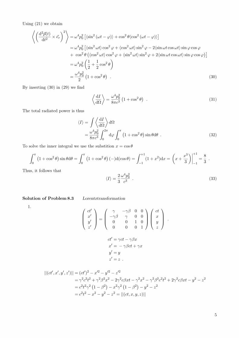
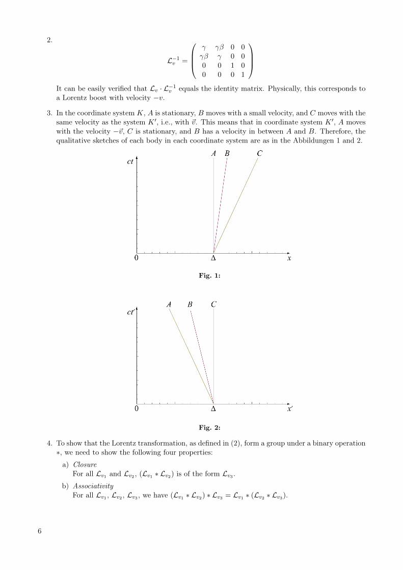
3. In the coordinate system K, A is stationary, B moves with a small velocity, and C moves with thesame velocity as the system K ′, i.e., with ~v. This means that in coordinate system K ′, A moveswith the velocity −~v, C is stationary, and B has a velocity in between A and B. Therefore, thequalitative sketches of each body in each coordinate system are as in the Abbildungen 1 and 2.

Fig. 1:

Fig. 2:

4. To show that the Lorentz transformation, as defined in (2), form a group under a binary operation∗, we need to show the following four properties:

a) ClosureFor all Lv1 and Lv2 , (Lv1 ∗ Lv2) is of the form Lv3 .

b) AssociativityFor all Lv1 , Lv2 , Lv3 , we have (Lv1 ∗ Lv2) ∗ Lv3 = Lv1 ∗ (Lv2 ∗ Lv3).

6

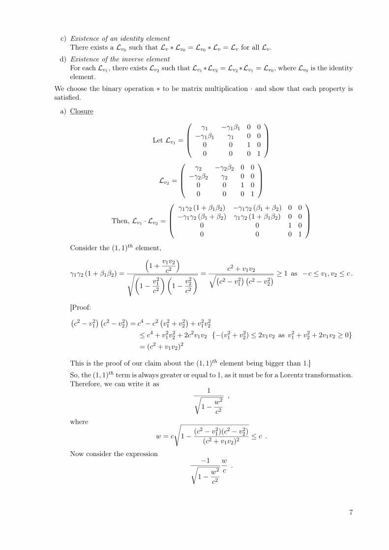
c) Existence of an identity elementThere exists a Lv0 such that Lv ∗ Lv0 = Lv0 ∗ Lv = Lv for all Lv.

d) Existence of the inverse elementFor each Lv1 , there exists Lv2 such that Lv1 ∗Lv2 = Lv2 ∗Lv1 = Lv0 , where Lv0 is the identityelement.

We choose the binary operation ∗ to be matrix multiplication · and show that each property issatisfied.

a) Closure

Let Lv1 =

γ1 −γ1β1 0 0−γ1β1 γ1 0 0

0 0 1 00 0 0 1

Lv2 =

γ2 −γ2β2 0 0−γ2β2 γ2 0 0

0 0 1 00 0 0 1

Then, Lv1 · Lv2 =

γ1γ2 (1 + β1β2) −γ1γ2 (β1 + β2) 0 0−γ1γ2 (β1 + β2) γ1γ2 (1 + β1β2) 0 0

0 0 1 00 0 0 1

Consider the (1, 1)th element,

γ1γ2 (1 + β1β2) =

(1 +

v1v2c2

)√(

1− v21c2

)(1− v22

c2

) =c2 + v1v2√(

c2 − v21) (c2 − v22

) ≥ 1 as −c ≤ v1, v2 ≤ c .

[Proof:(c2 − v21

) (c2 − v22

)= c4 − c2

(v21 + v22

)+ v21v

22

≤ c4 + v21v22 + 2c2v1v2 −(v21 + v22) ≤ 2v1v2 as v21 + v22 + 2v1v2 ≥ 0

= (c2 + v1v2)2

This is the proof of our claim about the (1, 1)th element being bigger than 1.]

So, the (1, 1)th term is always greater or equal to 1, as it must be for a Lorentz transformation.Therefore, we can write it as

1√1− w2

c2

,

where

w = c

√1− (c2 − v21)(c2 − v22)

(c2 + v1v2)2≤ c .

Now consider the expression−1√

1− w2

c2

w

c.

7

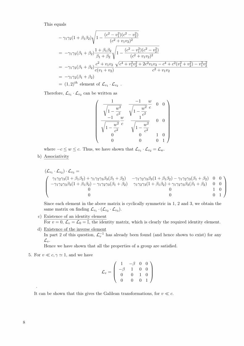
This equals

− γ1γ2(1 + β1β2)

√1− (c2 − v21)(c2 − v22)

(c2 + v1v2)2

= −γ1γ2(β1 + β2)1 + β1β2β1 + β2

√1− (c2 − v21)(c2 − v22)

(c2 + v1v2)2

= −γ1γ2(β1 + β2)c2 + v1v2c(v1 + v2)

√c4 + v21v

22 + 2c2v1v2 − c4 + c2(v21 + v22)− v21v22

c2 + v1v2

= −γ1γ2(β1 + β2)

= (1, 2)th element of Lv1 · Lv2 .

Therefore, Lv1 · Lv2 can be written as

1√1− w2

c2

−1√1− w2

c2

w

c0 0

−1√1− w2

c2

w

c

1√1− w2

c2

0 0

0 0 1 00 0 0 1

where −c ≤ w ≤ c. Thus, we have shown that Lv1 · Lv2 = Lw.

b) Associativity

(Lv1 · Lv2) · Lv3 =γ1γ2γ3(1 + β1β2) + γ1γ2γ3β3(β1 + β2) −γ1γ2γ3β3(1 + β1β2)− γ1γ2γ3(β1 + β2) 0 0−γ1γ2γ3β3(1 + β1β2)− γ1γ2γ3(β1 + β2) γ1γ2γ3(1 + β1β2) + γ1γ2γ3β3(β1 + β2) 0 0

0 0 1 00 0 0 1

Since each element in the above matrix is cyclically symmetric in 1, 2 and 3, we obtain thesame matrix on finding Lv1 · (Lv2 · Lv3).

c) Existence of an identity elementFor v = 0, Lv = L0 = I, the identity matrix, which is clearly the required identity element.

d) Existence of the inverse elementIn part 2 of this question, L−1v has already been found (and hence shown to exist) for anyLv.Hence we have shown that all the properties of a group are satisfied.

5. For v c, γ ' 1, and we have

Lv =

1 −β 0 0−β 1 0 00 0 1 00 0 0 1

.

It can be shown that this gives the Galilean transformations, for v c.

8

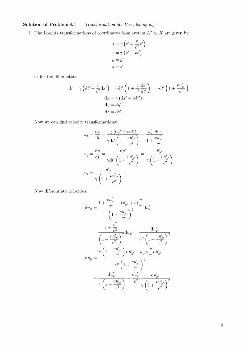
Solution of Problem8.4 Transformation der Beschleunigung

1. The Lorentz transformations of coordinates from system K ′ to K are given by:

t = γ(t′ +

v

c2x′)

x = γ(x′ + vt′

)y = y′

z = z′

or for the differentials

dt = γ(

dt′ +v

c2dx′)

= γdt′(

1 +v

c2dx′

dt′

)= γdt′

(1 +

vu′x′

c2

)dx = γ

(dx′ + vdt′

)dy = dy′

dz = dz′ .

Now we can find velocity transformations:

ux =dx

dt=

γ (dx′ + vdt′)

γdt′(

1 +vu′x′

c2

) =u′x′ + v

1 +vu′x′

c2

uy =dy

dt=

dy′

γdt′(

1 +vu′x′

c2

) =u′y′

γ

(1 +

vu′x′

c2

)uz =

u′z′

γ

(1 +

vu′x′

c2

) .

Now diferentiate velocities:

dux =1 +

vu′x′

c2− (u′x′ + v)

v

c2(1 +

vu′x′

c2

)2 du′x′

=1− v2

c2(1 +

vu′x′

c2

)2du′x′ =du′x′

γ2(

1 +vu′x′

c2

)2

duy =

γ

(1 +

vu′x′

c2

)du′y′ − u′y′γ

v

c2du′x′

γ2(

1 +vu′x′

c2

)2

=du′y′

γ

(1 +

vu′x′

c2

) − vu′y′

c2du′x′

γ

(1 +

vu′x′

c2

)2 ,

9

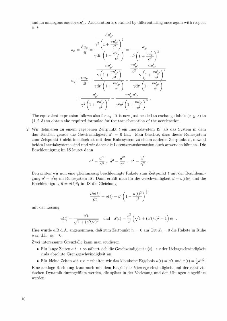
and an analogous one for du′z′ . Acceleration is obtained by differentiating once again with respectto t:

ax =duxdt

=

du′x′

γ2(

1 +vu′x′

c2

)2

γdt′(

1 +vu′x′

c2

) =a′x′

γ3(

1 +vu′x′

c2

)3

ay =duydt

=

du′y′

γ

(1 +

vu′x′

c2

)γdt′

(1 +

vu′x′

c2

) −vu′y′

c2du′x′

γ

(1 +

vu′x′

c2

)2

γdt′(

1 +vu′x′

c2

)=

a′y′

γ2(

1 +vu′x′

c2

)2 −vu′y′a

′x′

γ2c2(

1 +vu′x′

c2

)3 .

The equivalent expression follows also for az. It is now just needed to exchange labels (x, y, z) to(1, 2, 3) to obtain the required formulae for the transformation of the acceleration.

2. Wir definieren zu einem gegebenen Zeitpunkt t ein Inertialsystem IS’ als das System in demdas Teilchen gerade die Geschwindigkeit ~u′ = 0 hat. Man beachte, dass dieses Ruhesystemzum Zeitpunkt t nicht identisch ist mit dem Ruhesystem zu einem anderen Zeitpunkt t′, obwohlbeides Inertialsysteme sind und wir daher die Lorentztransformation auch anwenden können. DieBeschleunigung im IS lautet dann

a1 =a′1

γ3, a2 =

a′2

γ2, a2 =

a′3

γ2.

Betrachten wir nun eine gleichmässig beschleunigte Rakete zum Zeitpunkt t mit der Beschleuni-gung ~a′ = a′~e1 im Ruhesystem IS’. Dann erhält man für die Geschwindigkeit ~u = u(t)~e1 und dieBeschleunigung ~a = a(t)~e1 im IS die Gleichung

∂u(t)

∂t= a(t) = a′

(1− u(t)2

c2

) 32

mit der Lösung

u(t) =a′t√

1 + (a′t/c)2und ~x(t) =

c2

a′

(√1 + (a′t/c)2 − 1

)~e1 .

Hier wurde o.B.d.A. angenommen, daß zum Zeitpunkt t0 = 0 am Ort ~x0 = 0 die Rakete in Ruhewar, d.h. u0 = 0.

Zwei interessante Grenzfälle kann man studieren

• Für lange Zeiten a′t→∞ nähert sich die Geschwindigkeit u(t)→ c der Lichtgeschwindigkeitc als absolute Grenzgeschwindigkeit an.

• Für kleine Zeiten a′t << c erhalten wir das klassische Ergebnis u(t) = a′t und x(t) = 12a′t2.

Eine analoge Rechnung kann auch mit dem Begriff der Vierergeschwindigkeit und der relativis-tischen Dynamik durchgeführt werden, die später in der Vorlesung und den Übungen eingeführtwerden.

10