Embed Size (px)
Citation preview
Que
llena
ngab
e
1Que
llena
ngab
e
1Institut für Hochfrequenztechnk und Radar W. Keydel, Vorlesung IHFT Erlangen
8. Grundlagen der SAR Polarimetrie
Vorlesung: Hochauflösende RadarsystemeWS 2007/08,
Friedrich-Alexander-Universität Erlangen NürnbergLehrstuhl für Hochfrequenztechnik
Wolfgang KeydelDLR Oberpfaffenhofen, Institut für Hochfrequenztechnik und Radarsysteme
e-mail: [email protected], Web: http://www.keydel.com
Literatur: Martin Hellmann, SAR Polarimetry, Tutorialhttp://www.fpk.tu-berlin.de/~anderl/epsilon/polarimetrytutorial.pdf
Keydel, W. (Editor) Radar Polarimetry and Interferometry Lecture Series RTO-EN-SET-081 Radar Interferometry and Polarimetry
http://www.rta.nato.int/panel.asp?panel=SET&O=RTOPubNumber#
Que
llena
ngab
e
2Que
llena
ngab
e
2Institut für Hochfrequenztechnk und Radar W. Keydel, Vorlesung IHFT Erlangen
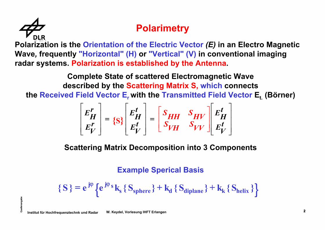
PolarimetryPolarization is the Orientation of the Electric Vector (E) in an Electro Magnetic Wave, frequently "Horizontal" (H) or "Vertical" (V) in conventional imaging radar systems. Polarization is established by the Antenna.
Complete State of scattered Electromagnetic Wave described by the Scattering Matrix S, which connects
the Received Field Vector Er with the Transmitted Field Vector Et. (Börner)
Scattering Matrix Decomposition into 3 Components
Example Sperical Basis
EHr
EVr {S}
EHt
EVt
SHH SHVSVH SVV
EHt
EVt
L
NMMM
O
QPPP
=L
NMMM
O
QPPP
=LNMM
OQPPL
NMMM
O
QPPP
{ } { } { } { }S e e k S k S k Sj j ss sphere d diplane k helix= + +ϕ ϕn s
Que
llena
ngab
e
3Que
llena
ngab
e
3Institut für Hochfrequenztechnk und Radar W. Keydel, Vorlesung IHFT Erlangen
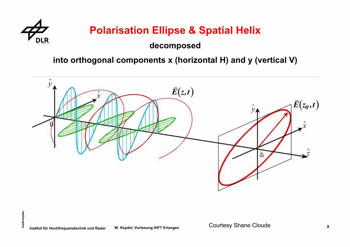
Polarisation Ellipse & Spatial Helixdecomposed
into orthogonal components x (horizontal H) and y (vertical V)
Courtesy Shane Cloude
Que
llena
ngab
e
4Que
llena
ngab
e
4Institut für Hochfrequenztechnk und Radar W. Keydel, Vorlesung IHFT Erlangen
Que
llena
ngab
e
5Que
llena
ngab
e
5Institut für Hochfrequenztechnk und Radar W. Keydel, Vorlesung IHFT Erlangen
X
Y
RXAX
RY
AY
YXS
XXS
YYS
XYS
YXS
XXS
YYS
XYS
X Y X Y
RX
RY
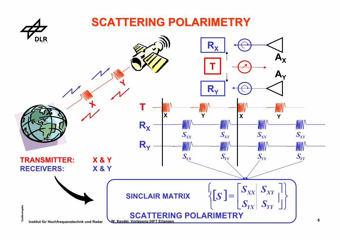
SCATTERING POLARIMETRYSCATTERING POLARIMETRY
TRANSMITTER: X & YRECEIVERS: X & Y
TT
T
SINCLAIR MATRIX
SCATTERING POLARIMETRY
[ ]⎭⎬⎫
⎩⎨⎧
⎥⎦
⎤⎢⎣
⎡=
YY
XY
YX
XX
SS
SS
S

Que
llena
ngab
e
6Que
llena
ngab
e
6Institut für Hochfrequenztechnk und Radar W. Keydel, Vorlesung IHFT Erlangen
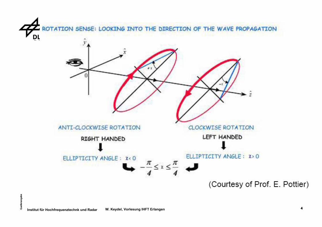
Polarization Ellipse
χ = Ellipticity Angle: 0 ≤ χ ≤ π/4
Ψ= Orientation Angle: - π/2 ≤ ψ ≤ π/2
ξχ
Ψx
y
majoraxis
minor axis
η
αa ξ
aη
Ev
EX0
EY0
( ) ( ) ( ) cos)2tan()2tan(andsin2sin2sin
aa
)tan(andcosEEEE2
)2tan( 020y
20x
0x0y
ϕαψϕαχ
χϕψηξ
ξ
==
±=−
=
withsincosEEEE
2EE
EE
yx0000x0y
xy2
0x
x
2
0y
y ϕϕϕϕϕ −==⎟⎟⎠
⎞⎜⎜⎝
⎛−⎟⎟
⎠
⎞⎜⎜⎝
⎛+⎟⎟
⎠
⎞⎜⎜⎝
⎛
rrr
rrr
rrr
yjjkz
0yjkz
yy eee)z(Ee)z(E)z(E yϕ==
xjjkz
0xjkz
xx eee)z(Ee)z(E)z(E xϕ==
yyxx e)z(Ee)z(E)z(E +=
Que
llena
ngab
e
7Que
llena
ngab
e
7Institut für Hochfrequenztechnk und Radar W. Keydel, Vorlesung IHFT Erlangen
x
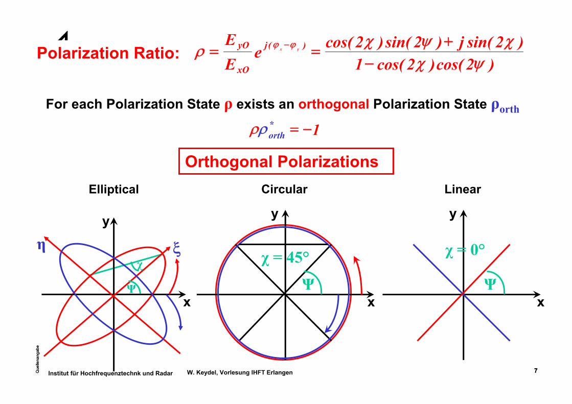
Polarization Ratio:
For each Polarization State ρ exists an orthogonal Polarization State ρorth
)2cos()2cos(1)2sin(j)2sin()2cos(e
EE )(j
xO
yO yx
ψχχψχρ ϕϕ
−+
== −
1*orth −=ρρ
Ψ
χ = 45°
x
y
Ψ
χ = 0°
y
Orthogonal PolarizationsCircular LinearElliptical
χ
Ψ
y
x
ξη

Que
llena
ngab
e
8Que
llena
ngab
e
8Institut für Hochfrequenztechnk und Radar W. Keydel, Vorlesung IHFT Erlangen
Examples:[S] SINCLAIR Matrix
k Target VectorE Jones Vektorg Stokes Vector
[T] Coherency Matrix[C] Covariance Matrix
X
Y
DIFFERENT TARGET POLARIMETRIC
DESCRIPTORS
POLARIMETRIC DESCRIPTORSPOLARIMETRIC DESCRIPTORS
TRANSMITTER: X & YRECEIVERS: X & Y
Courtesy Eric Poitier

Que
llena
ngab
e
9Que
llena
ngab
e
9Institut für Hochfrequenztechnk und Radar W. Keydel, Vorlesung IHFT Erlangen
Streumatrix (Sinclaire Matrix)
EHscat SHHEH
inc SHVEVinc
EVscat SVHEH
inc SVVEVinc
= +
= +
EscatEH
scat
EVscat
SHH SHVSVH SVV
EHinc
EVinc S(HV) Einc=
FHGGIKJJ =FHG
IKJFHGG
IKJJ =
Si ki ke
j i k,
, ,= σϕ
0
E kr e j t= − +E0e r−α
ω ϕ( )…α = jk +γ
8 unabhängige Parameter
Bei monostatischer Rückstreuung:SHV= SVH 5 Parameter
Que
llena
ngab
e
10Que
llena
ngab
e
10Institut für Hochfrequenztechnk und Radar W. Keydel, Vorlesung IHFT Erlangen
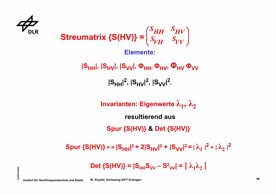
Streumatrix {S(HV)} = SHH SHVSVH SVV
FHG
IKJ
Elemente:
|SHH|, |SHV|, |SVV|, ΦHH, ΦHV, ΦHV ΦVV
|SHH|2, |SHV|2, |SVV|2,
Invarianten: Eigenwerte λ1, λ2
resultierend aus
Spur {S(HV)} & Det {S(HV)}
Spur {S(HV)} = = |SHH|2 + 2|SHV|2 + |SVV|2 = | λ1 |2 + | λ2 |2
Det {S(HV)} = |SHHSVV – S2VV| = | λ1λ2 |

Que
llena
ngab
e
11Que
llena
ngab
e
11Institut für Hochfrequenztechnk und Radar W. Keydel, Vorlesung IHFT Erlangen
Jones Vectorcomplete information about the Polarization Ellipse, except handleness!
r
With Polarisation Ratio ρ the Jones Vector can be written as:
⎥⎦
⎤⎢⎣
⎡=⎥
⎦
⎤⎢⎣
⎡=
ρ1
EEE
E xy
xxyr
⎥⎦
⎤⎢⎣
⎡=⎥
⎦
⎤⎢⎣
⎡=
y
x
j0y
j0x
y
xxy eE
eEEE
E ϕ
ϕr
yyxx e)z(Ee)z(E)z(E += r r
r
Two plane waves propagating in opposite directiond havethe same Jones Vector
Using the subscripts „ + “ and „-“ compensates this lack of consistency
Subscript „ + “ : propagation in +k direction, Subscript „ - “ : propagation in - k direction,
r
}{ }{ )rkt(j)rkt(j eERe)t(,E & eERe)t(,Errrr rrrr +
−−−
++ == ωω
Que
llena
ngab
e
12Que
llena
ngab
e
12Institut für Hochfrequenztechnk und Radar W. Keydel, Vorlesung IHFT Erlangen
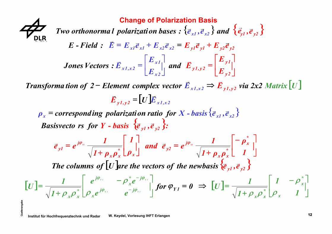
Change of Polarization Basis{ } { }
[ ]
[ ] {
0for
newbasistheofvectorstheareUofcolumnsThe
e,eande,e:basesonpolarizatilorthonormaTwo
1Y
y2y1x2x1
⇒=
eEeEeEeEE:Field-E y2y2y1y1x2x2x1x1 +=+=
[ ]1
11
1Ux
*x
*xx
⎥⎦
⎤⎢⎣
⎡ −
+=
ρρ
ρρϕ[ ]
eeee
11U jj
x
j*x
j
*xx
1Y1Y
1Y1Y
⎥⎦
⎤⎢⎣
⎡ −
+=
−
−
ρρ
ρρ ϕϕ
ϕϕ
}e,e y2y1rr
1ρ
ρρ11eeand
ρ1
ρρ11ee
*x
*xx
jy2
x*xx
jy1
Y2Y1 ⎥⎦
⎤⎢⎣
⎡−
+=⎥
⎦
⎤⎢⎣
⎡
+= ϕϕ rr
{ }:e,ebasis-YforrsBasisvecto y2y1rr
{ }e,ebasis-Xforratioonpolarizatiingcorrespondρ x2x1x = rr
[ ]EUE
UMatrix via 2x2EEvectorcomplexElement2oftionTransforma
2x,1x2y,1y
2y,1y2x,1x
=
⇒−rr
rrEE
EandEE
E:VectorsonesJ2y
1y2y,1y
2x
1x2x,1x ⎥
⎦
⎤⎢⎣
⎡=⎥
⎦
⎤⎢⎣
⎡=
rr
rrrrr
rrrr

Que
llena
ngab
e
13Que
llena
ngab
e
13Institut für Hochfrequenztechnk und Radar W. Keydel, Vorlesung IHFT Erlangen Courtesy Eric Poitier
x x
xx
y
y y
y
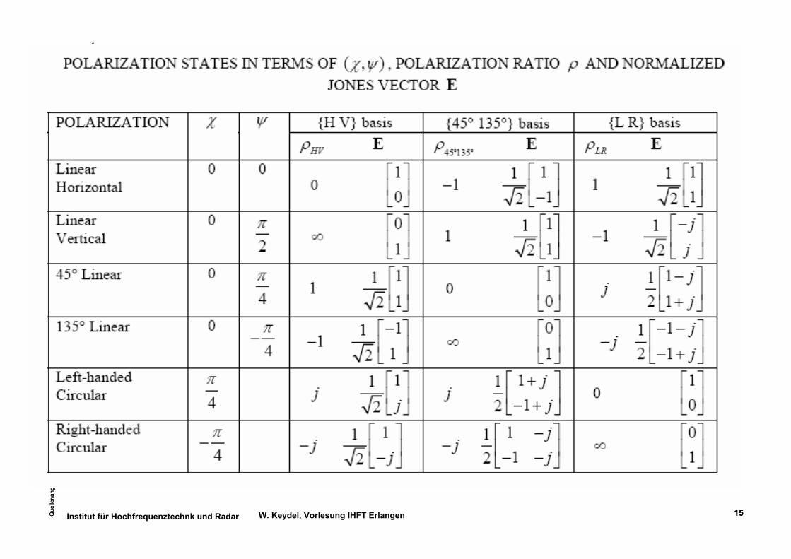
Jones Vector Descriptions for Characteristic Polarization States
Propagation Direction out of Page
Que
llena
ngab
e
14Que
llena
ngab
e
14Institut für Hochfrequenztechnk und Radar W. Keydel, Vorlesung IHFT Erlangen
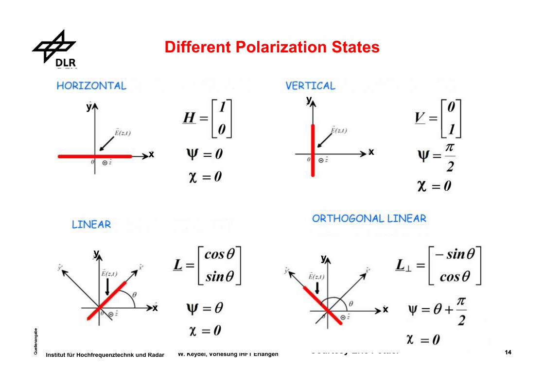
Different Polarization States
Courtesy Eric Pottier
x x
xx
y
yy
y
Que
llena
ngab
e
15Que
llena
ngab
e
15Institut für Hochfrequenztechnk und Radar W. Keydel, Vorlesung IHFT Erlangen

Que
llena
ngab
e
16Que
llena
ngab
e
16Institut für Hochfrequenztechnk und Radar W. Keydel, Vorlesung IHFT Erlangen
Poincarés Polarization Sphere
Courtesy Eric Poitier

Que
llena
ngab
e
17Que
llena
ngab
e
17Institut für Hochfrequenztechnk und Radar W. Keydel, Vorlesung IHFT Erlangen
Poincare Sphere
Ellip
ticity
Ang
le χ
Orientation Angle Ψ
Que
llena
ngab
e
18Que
llena
ngab
e
18Institut für Hochfrequenztechnk und Radar W. Keydel, Vorlesung IHFT Erlangen
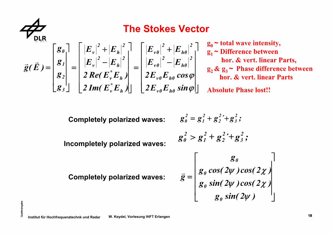
The Stokes Vector
⎥⎥⎥⎥⎥
⎦
⎤
⎢⎢⎢⎢⎢
⎣
⎡
−+
=
⎥⎥⎥⎥⎥
⎦
⎤
⎢⎢⎢⎢⎢
⎣
⎡
−+
=
⎥⎥⎥⎥
⎦
⎤
⎢⎢⎢⎢
⎣
⎡
=
ϕϕ
sinEE2cosEE2EEEE
)EEIm(2)EERe(2
EEEE
gggg
)E(g
0h0v
0h0v
20h
20v
20h
20v
h*v
h*v
2h
2v
2h
2v
3
2
1
0
rr
;g´ggg 23
22
21
20 ++=
g0 ~ total wave intensity,g1 ~ Difference between
hor. & vert. linear Parts, g2 & g3 ~ Phase difference between
hor. & vert. linear Parts
Absolute Phase lost!!
Completely polarized waves:
Incompletely polarized waves:;g´ggg 2
322
21
20 ++>
Completely polarized waves:
⎥⎥⎥⎥
⎦
⎤
⎢⎢⎢⎢
⎣
⎡
=
)2sin(g)2cos()2sin(g)2cos()2cos(g
g
g
0
0
0
0
ψχψχψr

Que
llena
ngab
e
19Que
llena
ngab
e
19Institut für Hochfrequenztechnk und Radar W. Keydel, Vorlesung IHFT Erlangen
Depolarization Scheme
Que
llena
ngab
e
20Que
llena
ngab
e
20Institut für Hochfrequenztechnk und Radar W. Keydel, Vorlesung IHFT Erlangen
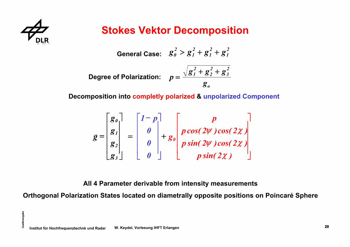
Stokes Vektor Decomposition
Degree of Polarization:o
23
22
21
gggg
p++
=
Decomposition into completly polarized & unpolarized Component
21
21
21
20 gggg ++>General Case:
⎥⎥⎥⎥
⎦
⎤
⎢⎢⎢⎢
⎣
⎡ −
000
p1
+=
⎥⎥⎥⎥
⎦
⎤
⎢⎢⎢⎢
⎣
⎡
gggg
3
2
1
0
⎥⎥⎥⎥
⎦
⎤
⎢⎢⎢⎢
⎣
⎡
)2sin(p)2cos()2sin(p)2cos()2cos(p
p
g0
χχψχψ
=gr
All 4 Parameter derivable from intensity measurements
Orthogonal Polarization States located on diametrally opposite positions on Poincaré Sphere

Que
llena
ngab
e
21Que
llena
ngab
e
21Institut für Hochfrequenztechnk und Radar W. Keydel, Vorlesung IHFT Erlangen
BasismatrizenEine generische Matrix ist in Basismatrizen zerlegbar;
Beispiel:
{S}S SS S
HH HV
VH VV= LNM
OQP
a b cc a b
a b c+
−LNM
OQP
= LNMOQP
+−
LNM
OQP
+ LNMOQP
1 00 1
1 00 1
0 11 0
a b S a b SHH VV+ = − =;
a S S b S S c S SHH VV HH VV HV VH= + = − = =; ;
Streuvektor (Target Vector) k = (a,b,c) = (SHH + SVV ; SHH - SVV ; 2SHV)
Que
llena
ngab
e
22Que
llena
ngab
e
22Institut für Hochfrequenztechnk und Radar W. Keydel, Vorlesung IHFT Erlangen
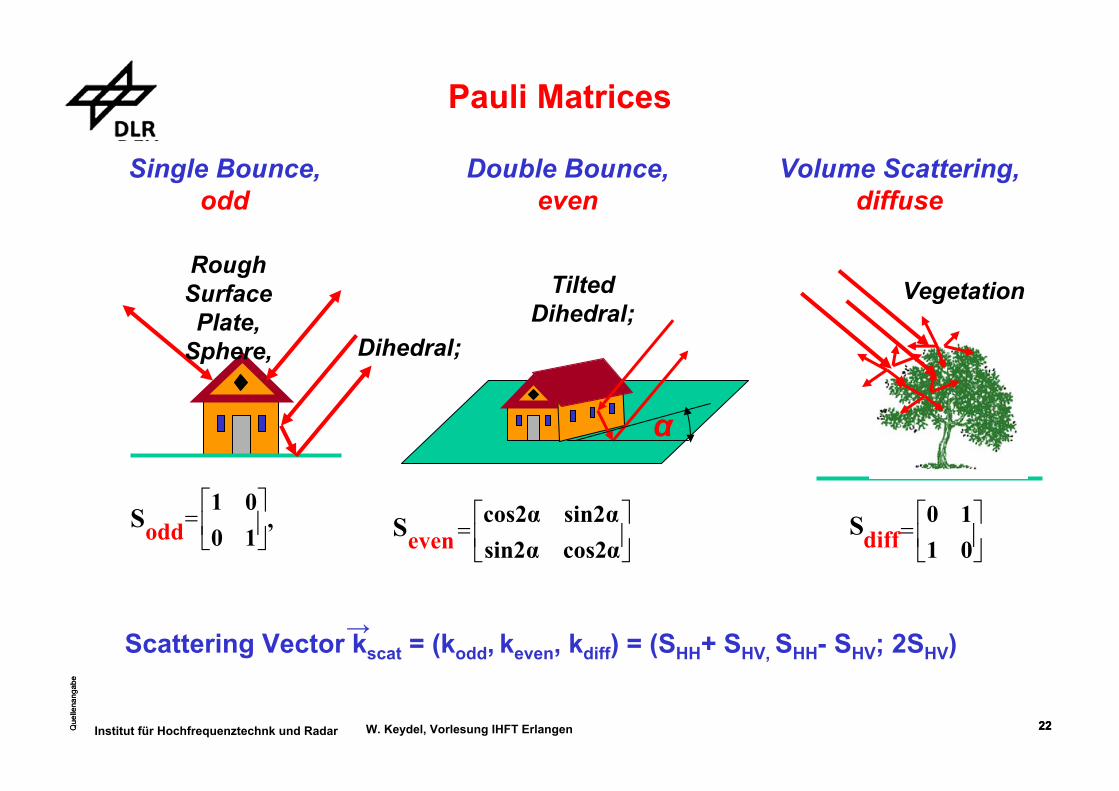
Pauli Matrices
RoughSurfacePlate,
Sphere, Dihedral;
TiltedDihedral;
α
Vegetation
⎥⎦
⎤⎢⎣
⎡=
0110Sdiff⎥
⎦
⎤⎢⎣
⎡= ,
1001Sodd ⎥
⎦
⎤⎢⎣
⎡=
cos2αsin2αsin2αcos2αSeven
Single Bounce, odd
Double Bounce, even
Volume Scattering,diffuse
Scattering Vector kscat = (kodd, keven, kdiff) = (SHH+ SHV, SHH- SHV; 2SHV)→
Que
llena
ngab
e
23Que
llena
ngab
e
23Institut für Hochfrequenztechnk und Radar W. Keydel, Vorlesung IHFT Erlangen
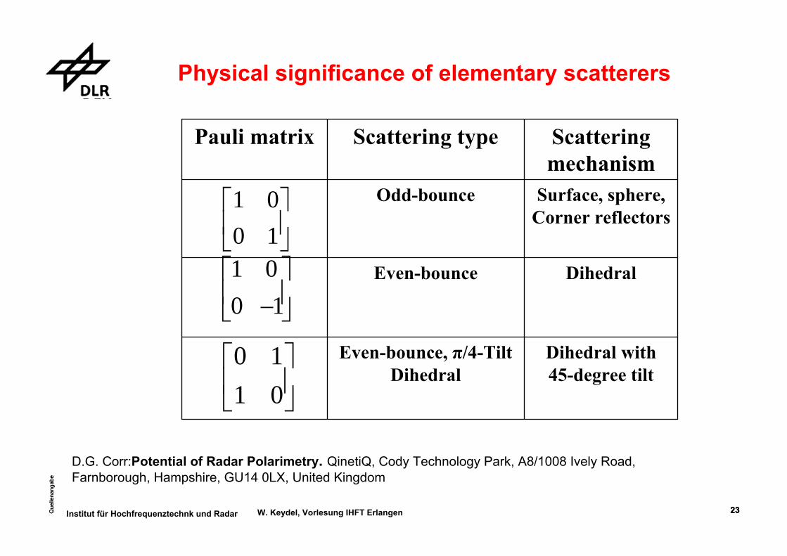
Dihedral with 45-degree tilt
Even-bounce, π/4-TiltDihedral
DihedralEven-bounce
Surface, sphere, Corner reflectors
Odd-bounce
Scattering mechanism
Scattering typePauli matrix
1 00 1
⎡ ⎤⎢ ⎥⎣ ⎦1 00 1
⎡ ⎤⎢ ⎥−⎣ ⎦
0 11 0
⎡ ⎤⎢ ⎥⎣ ⎦
Physical significance of elementary scatterers
D.G. Corr:Potential of Radar Polarimetry. QinetiQ, Cody Technology Park, A8/1008 Ively Road, Farnborough, Hampshire, GU14 0LX, United Kingdom
Que
llena
ngab
e
24Que
llena
ngab
e
24Institut für Hochfrequenztechnk und Radar W. Keydel, Vorlesung IHFT Erlangen
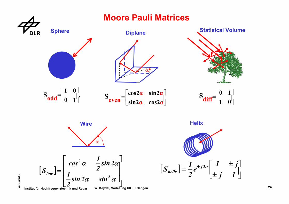
Moore Pauli Matrices
[ ]⎥⎥⎥
⎦
⎤
⎢⎢⎢
⎣
⎡
=αα
αα
2
2
linesin2sin
21
2sin21cos
S
Sphere Statisical Volume
⎥⎦
⎤⎢⎣
⎡=
0110Sdiff⎥
⎦
⎤⎢⎣
⎡= ,
1001Sodd
Wire
α
⎥⎦
⎤⎢⎣
⎡=
cos2αsin2αsin2αcos2αSeven
Diplane
α
[ ] ⎥⎦
⎤⎢⎣
⎡±
±= ±
1jj1
e21S 2j
helixα
Helix

Que
llena
ngab
e
25Que
llena
ngab
e
25Institut für Hochfrequenztechnk und Radar W. Keydel, Vorlesung IHFT Erlangen
⎥⎦
⎤⎢⎣
⎡=⎥
⎦
⎤⎢⎣
⎡=⎥
⎦
⎤⎢⎣
⎡=
0110
S,cos2αsin2αsin2αcos2α
S,1001
S dfiffus21
Que
llena
ngab
e
26Que
llena
ngab
e
26Institut für Hochfrequenztechnk und Radar W. Keydel, Vorlesung IHFT Erlangen
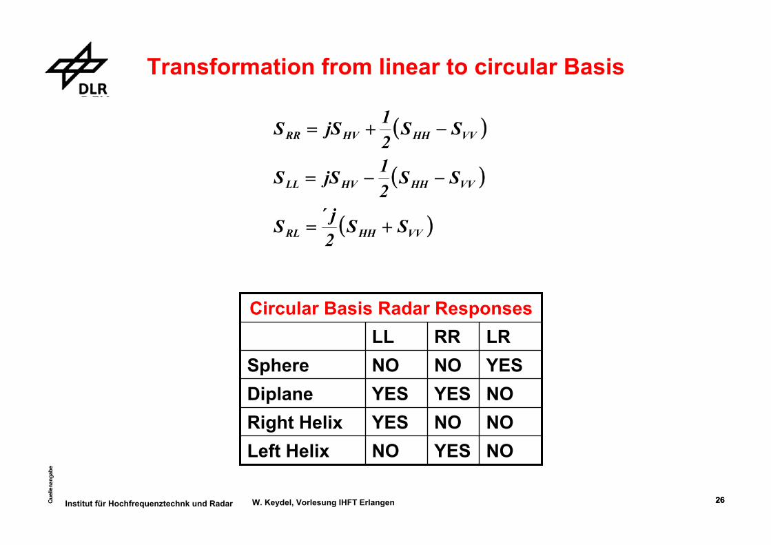
Transformation from linear to circular Basis
( )
( )
( )VVHHRL
VVHHHVLL
VVHHHVRR
SS2j´S
SS21jSS
SS21jSS
+=
−−=
−+=
Circular Basis Radar Responses
NOYESNOLeft HelixNONOYESRight HelixNOYESYESDiplaneYESNONOSphereLRRRLL
Que
llena
ngab
e
27Que
llena
ngab
e
27Institut für Hochfrequenztechnk und Radar W. Keydel, Vorlesung IHFT Erlangen
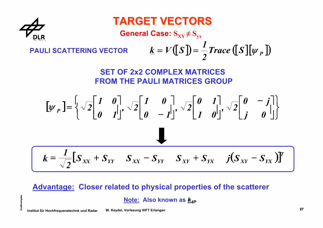
TARGET VECTORSTARGET VECTORS
PAULI SCATTERING VECTOR
Advantage: Closer related to physical properties of the scatterer
[ ]( ) [ ][ ]( )PSTrace21SVk ψ==
SET OF 2x2 COMPLEX MATRICES FROM THE PAULI MATRICES GROUP
Note: Also known as k4P
[ ]⎭⎬⎫
⎩⎨⎧
⎥⎦
⎤⎢⎣
⎡ −⎥⎦
⎤⎢⎣
⎡⎥⎦
⎤⎢⎣
⎡−⎥⎦
⎤⎢⎣
⎡=0j
j02,
0110
2,10
012,
1001
2Pψ
( )[ ]TYXXYYXXYYYXXYYXX SSjSSSSSS
21k −+−+=
General Case: SXY ≠ Syx

Que
llena
ngab
e
28Que
llena
ngab
e
28Institut für Hochfrequenztechnk und Radar W. Keydel, Vorlesung IHFT Erlangen
PAULI SCATTERING VECTOR k
COHERENCY MATRIX [T]
[ ]⎥⎥⎥⎥
⎦
⎤
⎢⎢⎢⎢
⎣
⎡
−+++−−−−+++−+−
=⋅=
A2jIJjNMjKLjIJBBjFEjGHjNMjFEBBjDCjKLjGHjDCA2
kkT0
0
0
T*
HERMITIAN POSITIVE SEMI DEFINITE MATRIX - RANK 1
COHERENCY MATRIXCOHERENCY MATRIXBISTATIC CASE
( )[ ]TYXXYYXXYYYXXYYXX SSjSSSSSS
21k −+−+= ; ; ;
Que
llena
ngab
e
29Que
llena
ngab
e
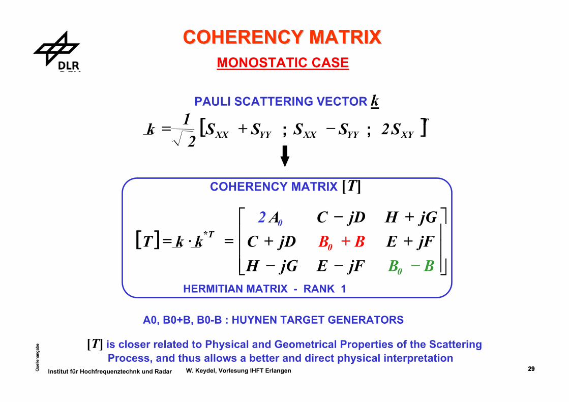
29Institut für Hochfrequenztechnk und Radar W. Keydel, Vorlesung IHFT Erlangen
HERMITIAN MATRIX - RANK 1
COHERENCY MATRIXCOHERENCY MATRIX
A0, B0+B, B0-B : HUYNEN TARGET GENERATORS
MONOSTATIC CASE
COHERENCY MATRIX [T]
[T] is closer related to Physical and Geometrical Properties of the ScatteringProcess, and thus allows a better and direct physical interpretation
PAULI SCATTERING VECTOR k
[ ]TXYYYXXYYXX S2SSSS2
1k −+= ;;
[ ]⎥⎥⎥
⎦
⎤
⎢⎢⎢
⎣
⎡
−−−++++−
=⋅=
BBjFEjGHjFEBBjDCjGHjDCA2
kkT
0
0
0T*
Que
llena
ngab
e
30Que
llena
ngab
e
30Institut für Hochfrequenztechnk und Radar W. Keydel, Vorlesung IHFT Erlangen
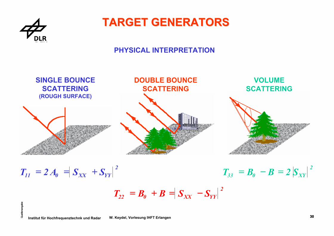
PHYSICAL INTERPRETATION
SINGLE BOUNCESCATTERING
(ROUGH SURFACE)
DOUBLE BOUNCESCATTERING
VOLUMESCATTERING
TARGET GENERATORS TARGET GENERATORS
2YYXX011 SSA2T +==
2YYXX022 SSBBT −=+=
2XY033 S2BBT =−=

Que
llena
ngab
e
31Que
llena
ngab
e
31Institut für Hochfrequenztechnk und Radar W. Keydel, Vorlesung IHFT Erlangen
Que
llena
ngab
e
32Que
llena
ngab
e
32Institut für Hochfrequenztechnk und Radar W. Keydel, Vorlesung IHFT Erlangen
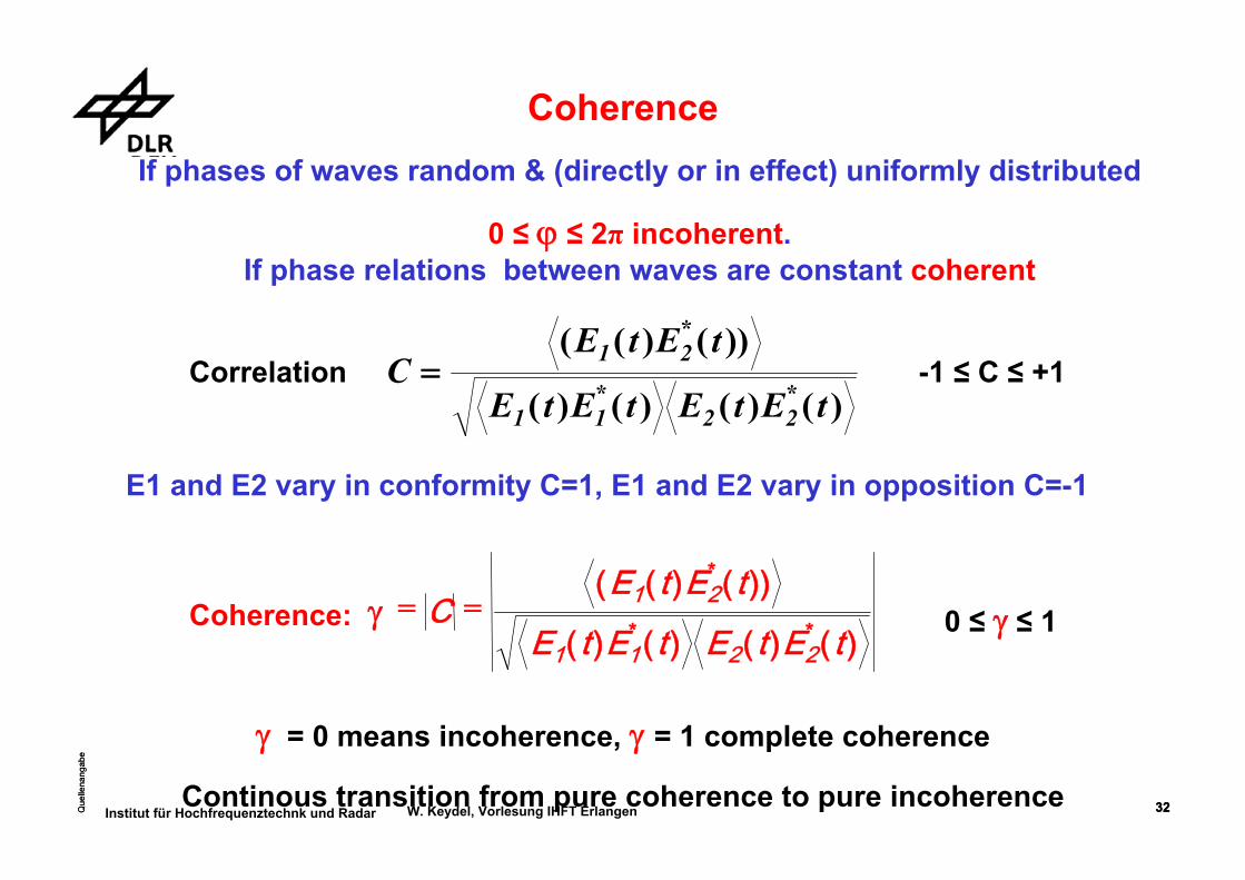
Coherence
CE t E t
E t E t E t E t=
( ( ) ( ))
( ) ( ) ( ) ( )
*
* *
1 2
1 1 2 2
E1 and E2 vary in conformity C=1, E1 and E2 vary in opposition C=-1
Coherence: γ = =CE t E t
E t E t E t E t( ( ) ( ))
( ) ( ) ( ) ( )
*
* *1 2
1 1 2 2
γ = 0 means incoherence, γ = 1 complete coherence
Continous transition from pure coherence to pure incoherence
If phases of waves random & (directly or in effect) uniformly distributed
0 ≤ ϕ ≤ 2π incoherent. If phase relations between waves are constant coherent
0 ≤ γ ≤ 1
-1 ≤ C ≤ +1Correlation
Que
llena
ngab
e
33Que
llena
ngab
e
33Institut für Hochfrequenztechnk und Radar W. Keydel, Vorlesung IHFT Erlangen
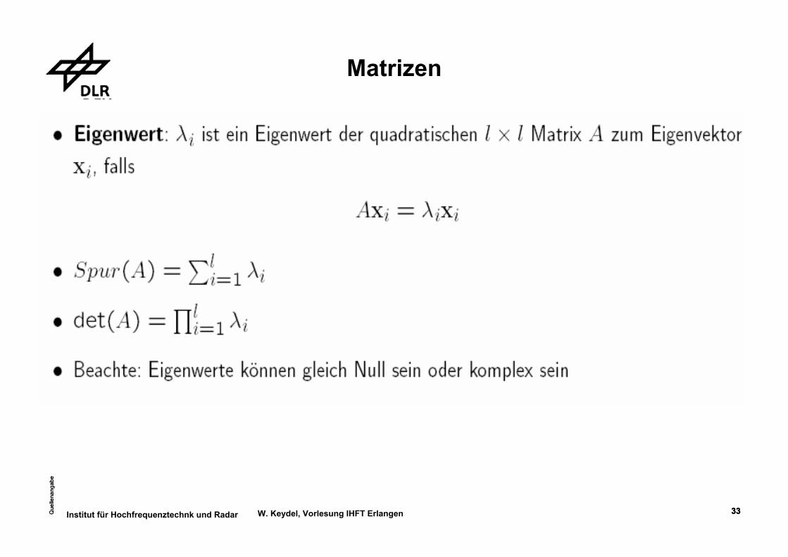
Matrizen
Que
llena
ngab
e
34Que
llena
ngab
e
34Institut für Hochfrequenztechnk und Radar W. Keydel, Vorlesung IHFT Erlangen
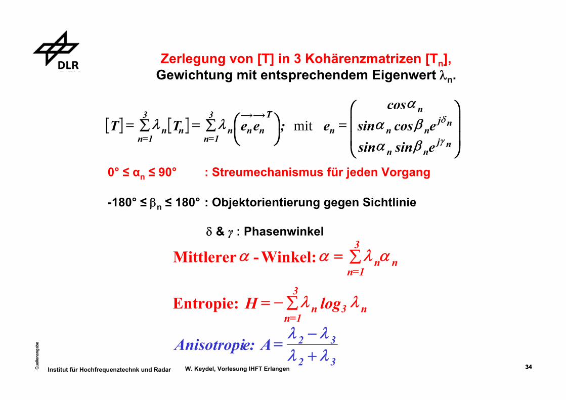
Zerlegung von [T] in 3 Kohärenzmatrizen [Tn],Gewichtung mit entsprechendem Eigenwert λn.
T T e e e ee
nn
n nn
n n
T
n
n
n nj n
n nj n
= ∑ = ∑ FHIK =
F
HGG
I
KJJ= =
λ λα
α βα β
δ
γ1
3
1
3;
cossin cossin sin
mit
0° ≤ αn ≤ 90° : Streumechanismus für jeden Vorgang
-180° ≤ βn ≤ 180° : Objektorientierung gegen Sichtlinie
δ & γ : Phasenwinkel
Mittlerer - Winkel:α α λ α= ∑=
n nn 1
3
2 3
Entropie: λ λ= − ∑=
n nn
H 31
3log
λ λλ λ
=−+
Anisotropie A 2 3:

Que
llena
ngab
e
35Que
llena
ngab
e
35Institut für Hochfrequenztechnk und Radar W. Keydel, Vorlesung IHFT Erlangen
DIFFICULT MECHANISM DISCRIMINATION WHEN : H > 0.7
ANISOTROPY(EIGENVALUES SPECTRUM)
λ1 λ2 λ332
32Aλλλλ
+−
=
COMPLEMENTARY TO ENTROPY
DISCRIMINATION WHEN H > 0.7
ROLL INVARIANT
H / A / H / A / aa DECOMPOSITION DECOMPOSITION
Que
llena
ngab
e
36Que
llena
ngab
e
36Institut für Hochfrequenztechnk und Radar W. Keydel, Vorlesung IHFT Erlangen
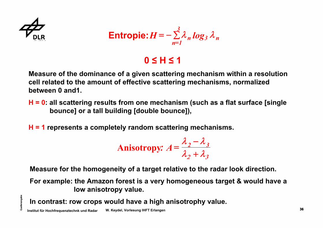
Measure for the homogeneity of a target relative to the radar look direction.
For example: the Amazon forest is a very homogeneous target & would have a low anisotropy value.
In contrast: row crops would have a high anisotrophy value.
λ λλ2 λ3
=−+
Anisotropy A 2 3:
0 ≤ H ≤ 1Measure of the dominance of a given scattering mechanism within a resolutioncell related to the amount of effective scattering mechanisms, normalizedbetween 0 and1.
H = 0: all scattering results from one mechanism (such as a flat surface [singlebounce] or a tall building [double bounce]),
H = 1 represents a completely random scattering mechanisms.
Entropie: λ λ= − ∑=
n nn
H 31
3log

Que
llena
ngab
e
37Que
llena
ngab
e
37Institut für Hochfrequenztechnk und Radar W. Keydel, Vorlesung IHFT Erlangen
H provides a measure of the diversity of the scattering mechanisms, degree of randomness statistical disorder
single mechanism H = 0, three mechanisms of equal power H = 1.
difficult mechanism discrimination when : H > 0.7
Eigenvalues Spectrum:
♣
Related to scattering mechanisms, not an orientation.Single bounce: α = 0; Double bounce: α = 90°; Diffuse scattering: α = 45°
Entropy: λ λ= ∑=
n nn
H 31
3logPolarimetric
- Angle:α α λ α= ∑=
n nn 1
3Mean
λ λλ2 λ3
=−+
Anisotropy A 2 3:λ1 λ2 λ3

Que
llena
ngab
e
38Que
llena
ngab
e
38Institut für Hochfrequenztechnk und Radar W. Keydel, Vorlesung IHFT Erlangen Courtesi Yoshio Yamagucci

Que
llena
ngab
e
39Que
llena
ngab
e
39Institut für Hochfrequenztechnk und Radar W. Keydel, Vorlesung IHFT Erlangen
Coherence & Covariance Matrices
T kk
k k k k k
k k k k k
k k k k k
k S S k S S k S S S
CoherenceMatrix
Todd odd even odd diff
odd even even even diff
odd diff even diff diff
odd HH VV even HH VV diff HV VH HV
= =
L
N
MMMMM
O
Q
PPPPP= + = − = + =
*
* *
* *
* *
; ;
12
2
2
2
2
CovarianceMatrix C kS kS
T
S S S S S S S
S S S S S S SS S S S S S S
S S S S S S S
HH HH HV HH VH HH VV
HV HH HV HV VH HV VV
VH HH VH HV VH VH VV
VV HH VV HV VV VH VV
= =
L
N
* * *
* * *
* * *
* * *
2
2
2
2
MMMMMM
O
Q
PPPPPP=k S S S Ss HH VV HV VH; ; ;a f
Que
llena
ngab
e
40Que
llena
ngab
e
40Institut für Hochfrequenztechnk und Radar W. Keydel, Vorlesung IHFT Erlangen
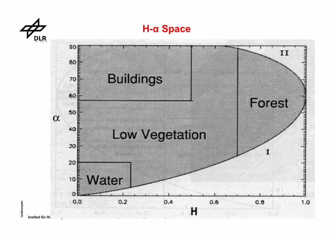
H-α Space

Que
llena
ngab
e
41Que
llena
ngab
e
41Institut für Hochfrequenztechnk und Radar W. Keydel, Vorlesung IHFT Erlangen
0 0.2 0.4 0.6 0.8 10
10
20
30
40
50
60
70
80
90
Entropy (H)
Alp
ha(α
)
9
3
LOWENTROPY
MEDIUMENTROPY
HIGHENTROPY
SURFACESCATTERING
VOLUMESCATTERING
MULTIPLESCATTERING
DIPOLE
DIHEDRAL SCATTERERFORESTRY DBLE BOUNCE
BRANCH / CROWNSTRUCTURE
CLOUD OF ANISOTROPICNEEDLES
NO FEASIBLEREGION
PERTURBATION OF 1st ORDERSCATTERING THEORIES DUE
TO 2nd ORDER EVENTS
DEGREE OF ARBITRARINESS(SCATTERING PROCESSES
RANDOM NOISE
1
47
2
65VEGETATION
8
SEGMENTATION OF THE H / α SPACE
H / A / H / A / αα DECOMPOSITION DECOMPOSITION
BRAGG SURFACE SURFACE ROUGHNESSPROPAGATION EFFECTS
Que
llena
ngab
e
42Que
llena
ngab
e
42Institut für Hochfrequenztechnk und Radar W. Keydel, Vorlesung IHFT Erlangen
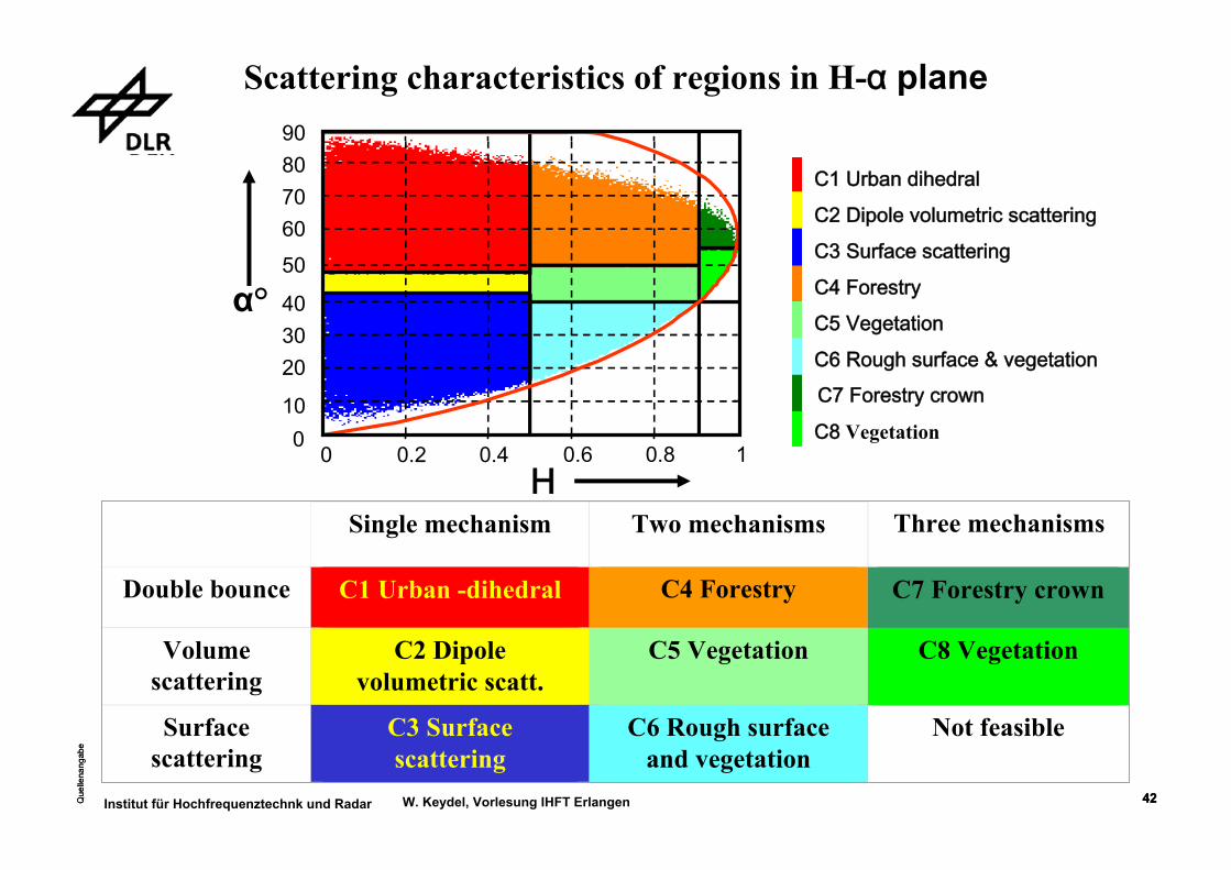
H
C1 Urban dihedral
C2 Dipole volumetric scattering
C3 Surface scattering
C4 Forestry C5 Vegetation
C6 Rough surface & vegetationC7 Forestry crown
C8 Vegetation
α°
C1 Urban -dihedral C4 Forestry C7 Forestry crown
C2 Dipole volumetric scatt.
C5 Vegetation C8 Vegetation
C3 Surface scattering
C6 Rough surface and vegetation
Single mechanism Two mechanisms Three mechanisms
Double bounce
Volume scattering
Surface scattering
Not feasible
Scattering characteristics of regions in H-α plane
0 0.2 0.4 0.6 0.8 10
10
203040
50
60708090
Que
llena
ngab
e
43Que
llena
ngab
e
43Institut für Hochfrequenztechnk und Radar W. Keydel, Vorlesung IHFT Erlangen
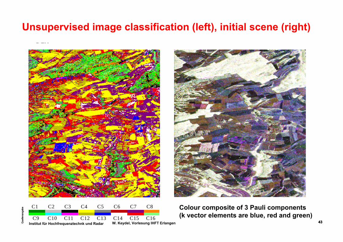
Unsupervised image classification (left), initial scene (right)
C9 C10 C11 C12 C13 C14 C15 C16
C1 C2 C3 C4 C5 C6 C7 C8 Colour composite of 3 Pauli components(k vector elements are blue, red and green)
Que
llena
ngab
e
44Que
llena
ngab
e
44Institut für Hochfrequenztechnk und Radar W. Keydel, Vorlesung IHFT Erlangen
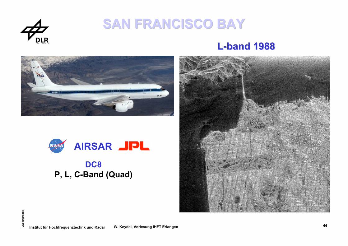
LL--band 1988 band 1988
SAN FRANCISCO BAYSAN FRANCISCO BAY
AIRSAR
DC8P, L, C-Band (Quad)

Que
llena
ngab
e
45Que
llena
ngab
e
45Institut für Hochfrequenztechnk und Radar W. Keydel, Vorlesung IHFT Erlangen
|HH+VV| |HV | |HH-VV|
TARGET GENERATORS TARGET GENERATORS
T11=2A0 T33=B0-B T22=B0+B

Que
llena
ngab
e
46Que
llena
ngab
e
46Institut für Hochfrequenztechnk und Radar W. Keydel, Vorlesung IHFT Erlangen
|HH+VV| |HV | |HH-VV|
TARGET GENERATORS TARGET GENERATORS
T11=2A0 T33=B0-B T22=B0+B|HH| |HV | |VV|
Sinclair Color Coding Pauli Color Coding
Que
llena
ngab
e
47Que
llena
ngab
e
47Institut für Hochfrequenztechnk und Radar W. Keydel, Vorlesung IHFT Erlangen
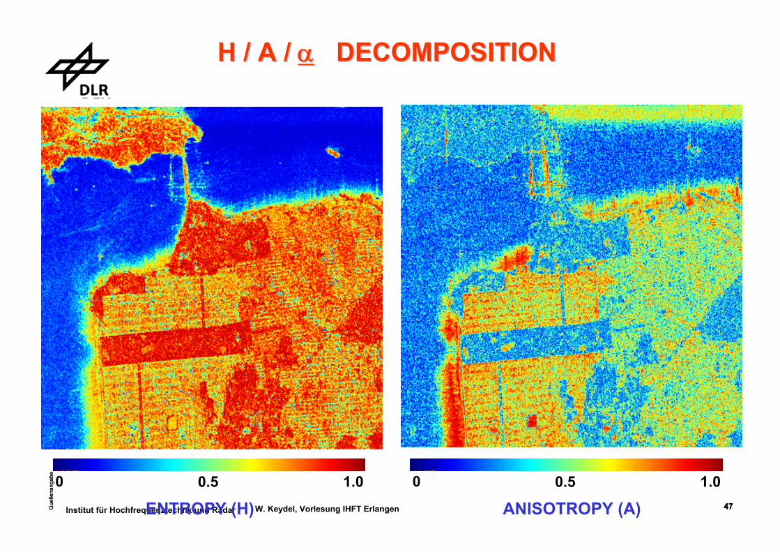
H / A / H / A / αα DECOMPOSITION DECOMPOSITION
ENTROPY (H)0.5 1.00
ANISOTROPY (A)0.5 1.00

Que
llena
ngab
e
48Que
llena
ngab
e
48Institut für Hochfrequenztechnk und Radar W. Keydel, Vorlesung IHFT Erlangen-15dB 0dB-30dB
( )dB0 BB + ( )dB0 BB −( )dB0A2
TARGET GENERATORSTARGET GENERATORS((TTiiii) )
Que
llena
ngab
e
49Que
llena
ngab
e
49Institut für Hochfrequenztechnk und Radar W. Keydel, Vorlesung IHFT Erlangen
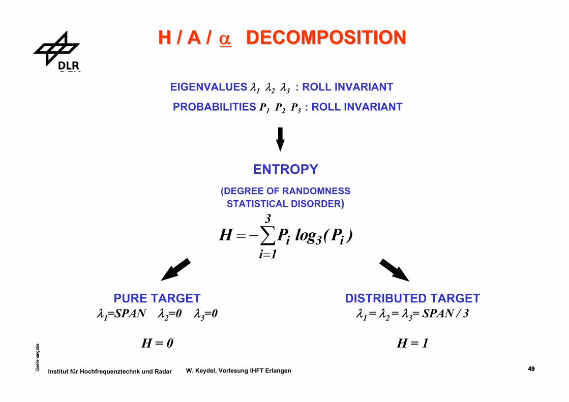
ENTROPY(DEGREE OF RANDOMNESS
STATISTICAL DISORDER)
H P Pi ii
= −=∑ log ( )3
1
3
DISTRIBUTED TARGETλ1 = λ2 = λ3= SPAN / 3
H = 1
PURE TARGETλ1=SPAN λ2=0 λ3=0
H = 0
EIGENVALUES λ1 λ2 λ3 : ROLL INVARIANT
PROBABILITIES P1 P2 P3 : ROLL INVARIANT
H / A /H / A / αα DECOMPOSITION DECOMPOSITION

Que
llena
ngab
e
50Que
llena
ngab
e
50Institut für Hochfrequenztechnk und Radar W. Keydel, Vorlesung IHFT Erlangen
0A2 BB0 + BB0 −
H / A / H / A / αα DECOMPOSITION DECOMPOSITION
ENTROPY (H)0.5 1.00

Que
llena
ngab
e
51Que
llena
ngab
e
51Institut für Hochfrequenztechnk und Radar W. Keydel, Vorlesung IHFT Erlangen
0A2 BB0 + BB0 −
H / A / H / A / αα DECOMPOSITION DECOMPOSITION
0 45° 90°
α PARAMETER
Que
llena
ngab
e
52Que
llena
ngab
e
52Institut für Hochfrequenztechnk und Radar W. Keydel, Vorlesung IHFT Erlangen
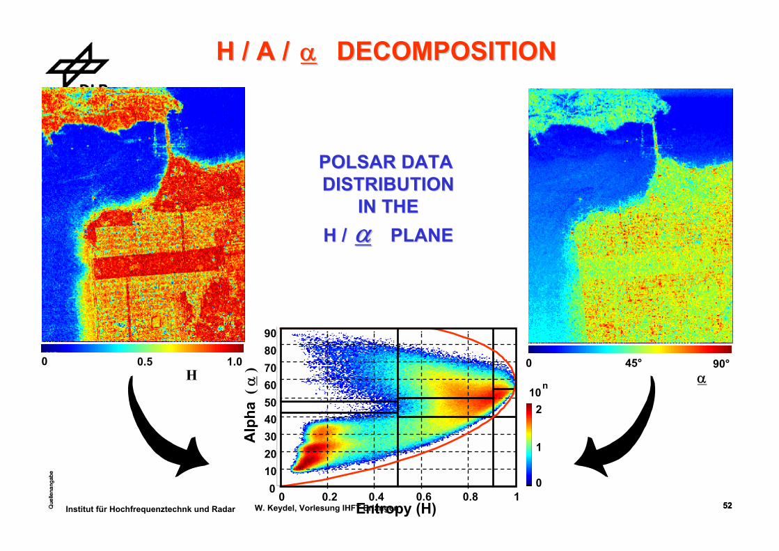
10n
0
1
2
H0.5 1.00
α0 45° 90°
Alp
ha( α
)
0 0.2 0.4 0.6 0.8 10
102030405060708090
Entropy (H)
H / A /H / A / αα DECOMPOSITION DECOMPOSITION
POLSAR DATA POLSAR DATA DISTRIBUTIONDISTRIBUTION
IN THEIN THEH /H / αα PLANEPLANE
Que
llena
ngab
e
53Que
llena
ngab
e
53Institut für Hochfrequenztechnk und Radar W. Keydel, Vorlesung IHFT Erlangen
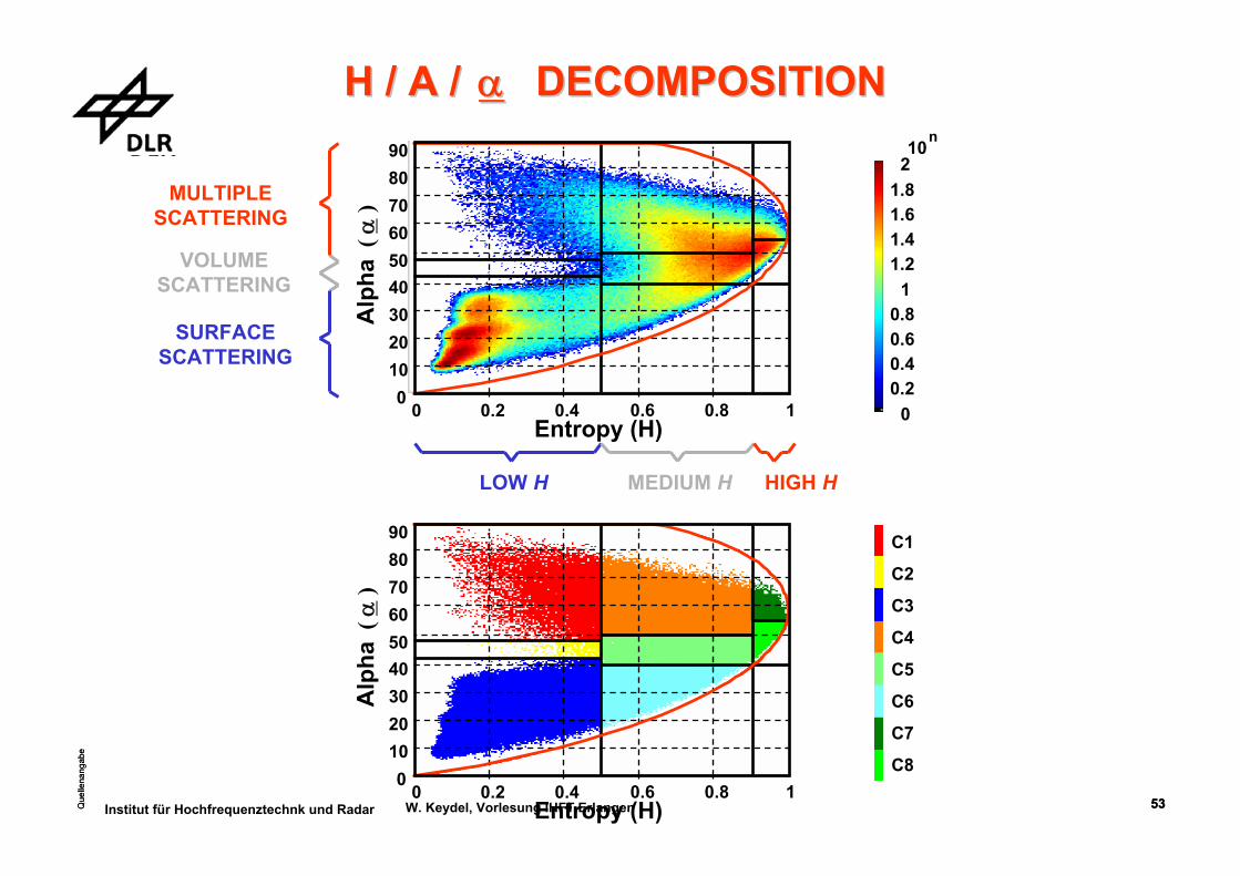
Alp
ha( α
)
0 0.2 0.4 0.6 0.8 10
102030405060708090
Entropy (H)
C1
C2
C3
C4
C5
C6
C7
C8
10n
00.20.40.60.8
11.21.41.61.8
2
LOW H MEDIUM H HIGH H
SURFACESCATTERING
VOLUMESCATTERING
MULTIPLESCATTERING
H / A /H / A / αα DECOMPOSITION DECOMPOSITION
Alp
ha( α
)
0 0.2 0.4 0.6 0.8 10
102030405060708090
Entropy (H)
Que
llena
ngab
e
54Que
llena
ngab
e
54Institut für Hochfrequenztechnk und Radar W. Keydel, Vorlesung IHFT Erlangen
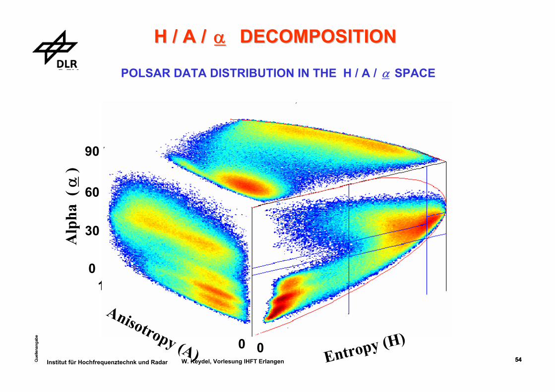
Alp
ha (
α)
0
30
60
90
0 0
0.50.5
11
POLSAR DATA DISTRIBUTION IN THE H / A / α SPACE
H / A /H / A / αα DECOMPOSITION DECOMPOSITION
Anisotropy (A) Entropy (H)

Que
llena
ngab
e
55Que
llena
ngab
e
55Institut für Hochfrequenztechnk und Radar W. Keydel, Vorlesung IHFT Erlangen
0A2 BB0 + BB0 −
H / A / H / A / αα DECOMPOSITION DECOMPOSITION H - α classification

Que
llena
ngab
e
56Que
llena
ngab
e
56Institut für Hochfrequenztechnk und Radar W. Keydel, Vorlesung IHFT Erlangen
332211 PPP αααα ++=
ENTROPY
)P(logPH3
1ii3i∑
=
−=
3 ROLL INVARIANT PARAMETERS
ANISOTROPY
32
32Aλλλλ
+−
=
α PARAMETER
( )( )
( )( )⎥⎥⎥⎥⎥⎥
⎦
⎤
⎢⎢⎢⎢⎢⎢
⎣
⎡
−−−
−=
AHAH
AHAH
I
111
1
α PHYSICAL SCATTERING MECHANISM
TYPE OF SCATTERING PROCESS
SEGMENTATION / CLASSIFICATION
H / A /H / A / αα DECOMPOSITION DECOMPOSITION
Que
llena
ngab
e
57Que
llena
ngab
e
57Institut für Hochfrequenztechnk und Radar W. Keydel, Vorlesung IHFT Erlangen
Polarimetric Analysis of Radar Signature ofa Manmade Structure
J.S. Lee, T. Ainsworth,NRL, Washington DC 20375, USA
Ernst Krogager, Danish Defence Research Establishment, Copenhagen,
Denmark
Wolfgang-Martin Boerner University of Illinois at Chicago, IL, USA
IGARSS 2006, Denver, Cororado, 2006

Que
llena
ngab
e
58Que
llena
ngab
e
58Institut für Hochfrequenztechnk und Radar W. Keydel, Vorlesung IHFT Erlangen
Pauli Vector, |HH-VV|, |HV|, |HH+VV|
Polarimetric SAR Image
EMISAR C-Band Polarimetric SAR Image of StoreBelt Bridge
RAN
GE
FLIGHT

Que
llena
ngab
e
59Que
llena
ngab
e
59Institut für Hochfrequenztechnk und Radar W. Keydel, Vorlesung IHFT Erlangen
Store Bridge Signature during Construction
|HH|
(A) |HH| image(B) |HV| image(C) |VV| image
Flight Direction
|HV|
|VV|
3
Que
llena
ngab
e
60Que
llena
ngab
e
60Institut für Hochfrequenztechnk und Radar W. Keydel, Vorlesung IHFT Erlangen
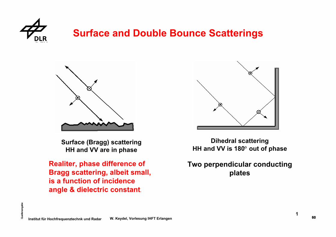
Surface and Double Bounce Scatterings
Surface (Bragg) scatteringHH and VV are in phase
Realiter, phase difference of Bragg scattering, albeit small, is a function of incidence angle & dielectric constant.
Dihedral scattering HH and VV is 180° out of phase
Two perpendicular conducting plates
1

Que
llena
ngab
e
61Que
llena
ngab
e
61Institut für Hochfrequenztechnk und Radar W. Keydel, Vorlesung IHFT Erlangen
Multi- Bounce Scattering
1 32
d
SingleDouble
Triple
Roundtrip distances:Single bounce return: Double bounce return:Triple bounce return:
θ is the local incidence angle.
)cos(2 θ− dL2L
)cos(2 θ+ dL
L
2
Que
llena
ngab
e
62Que
llena
ngab
e
62Institut für Hochfrequenztechnk und Radar W. Keydel, Vorlesung IHFT Erlangen
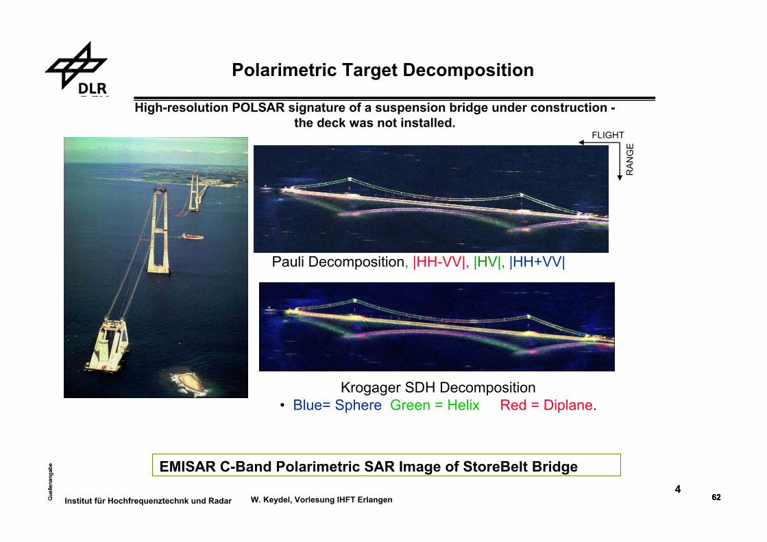
High-resolution POLSAR signature of a suspension bridge under construction -the deck was not installed.
Pauli Decomposition, |HH-VV|, |HV|, |HH+VV|
Aerial PhotoKrogager SDH Decomposition
• Blue= Sphere Green = Helix Red = Diplane.
RAN
GE
FLIGHT
Polarimetric Target Decomposition
EMISAR C-Band Polarimetric SAR Image of StoreBelt Bridge4
Que
llena
ngab
e
63Que
llena
ngab
e
63Institut für Hochfrequenztechnk und Radar W. Keydel, Vorlesung IHFT Erlangen
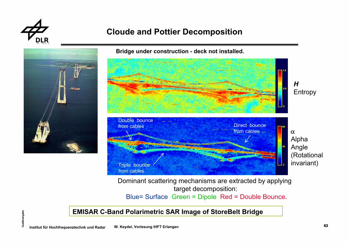
Bridge under construction - deck not installed.
Aerial Photo Dominant scattering mechanisms are extracted by applyingtarget decomposition:
Blue= Surface Green = Dipole Red = Double Bounce.
Cloude and Pottier Decomposition
EMISAR C-Band Polarimetric SAR Image of StoreBelt Bridge
Direct bounce from cables
Triple bounce from cables
Double bounce from cables
HEntropy
αAlphaAngle(Rotational invariant)
Que
llena
ngab
e
64Que
llena
ngab
e
64Institut für Hochfrequenztechnk und Radar W. Keydel, Vorlesung IHFT Erlangen
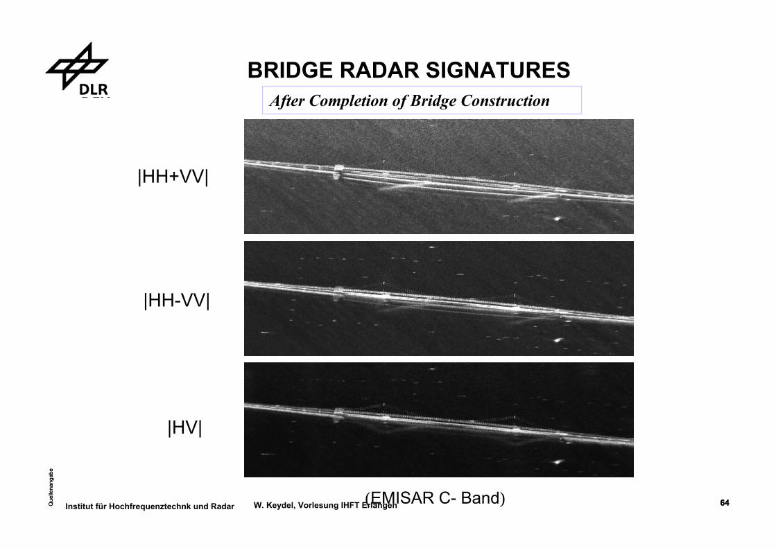
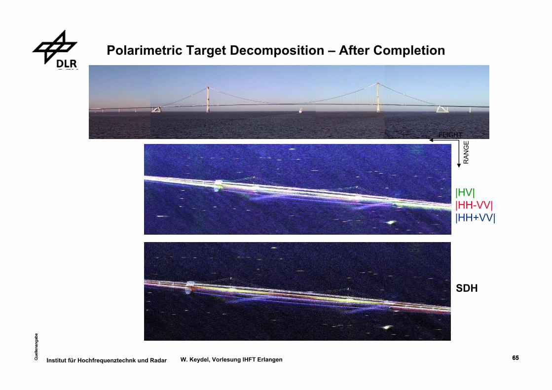
BRIDGE RADAR SIGNATURES
(EMISAR C- Band)
|HH+VV|
|HH-VV|
|HV|
After Completion of Bridge Construction
Que
llena
ngab
e
65Que
llena
ngab
e
65Institut für Hochfrequenztechnk und Radar W. Keydel, Vorlesung IHFT Erlangen
|HV||HH-VV||HH+VV|
RAN
GE
FLIGHT
Polarimetric Target Decomposition – After Completion
SDH

Que
llena
ngab
e
66Que
llena
ngab
e
66Institut für Hochfrequenztechnk und Radar W. Keydel, Vorlesung IHFT Erlangen
Entropy
Dominant scattering mechanisms are extracted by applying target decomposition: Blue= Surface Green = Dipole Red = Double Bounce.
Cloude and Pottier Decomposition – After Completion
Angle α
6

Que
llena
ngab
e
67Que
llena
ngab
e
67Institut für Hochfrequenztechnk und Radar W. Keydel, Vorlesung IHFT Erlangen
Dominant scattering mechanisms are extracted by applying target decomposition: Blue= Surface Green = Dipole Red = Double Bounce.
Higher Order Multiple Bounces – After Completion
αAlpha
Roundtrip distances:
A: Triple bounces,
B: 5 (or 7) bounces,
C: 7 (or 9) bounces,
D: 9 (or 11) bounces,(…) indicates additional two bounces from the bottom of the deck.
ddL 2)cos(2 ++ θ
)cos(2 θ+ dL
ddL 4)cos(2 ++ θ
ddL 6)cos(2 ++ θ
7
6c

Que
llena
ngab
e
68Que
llena
ngab
e
68Institut für Hochfrequenztechnk und Radar W. Keydel, Vorlesung IHFT Erlangen
BRIDGE AND BUOY RADAR SIGNATURES
Polarimetric SAR Image ( |HH-VV|, |HV|, |HH+VV| )
Navigation Map of Storebelt, Denmark
(EMISAR C- Band)

Que
llena
ngab
e
69Que
llena
ngab
e
69Institut für Hochfrequenztechnk und Radar W. Keydel, Vorlesung IHFT Erlangen
The Combination of Polarimetry and InterferometrySAR InterferometrySAR Polarimetry
Sensitive to scatterersshape, orientation and dielectric properties
Allows decomposition of different scattering processes
occurring inside the resolution cell
Established technique for terrain topography estimation
allows Location of scattering centers
inside the resolution cell
Polarimetric SAR InterferometryPotential to separate in height different scattering processes
occuring inside the resolution cell.
Sensitivity to the vertical distribution of the scattering mechanisms
Allows the investigation of 3D structure of volume scatterersrecovering co-registered textural plus spatial properties simultaneously
Phase sensitivity
Central Part: Coherence
Que
llena
ngab
e
70Que
llena
ngab
e
70Institut für Hochfrequenztechnk und Radar W. Keydel, Vorlesung IHFT Erlangen
Correlation:
Co-pol correlation provides a method to detect depolarization.
If the scattering is dominated by surface scattering, one wouldexpect high correlation and a phase difference approaching 0º.
In contrast, when depolarization occurs, due to volumescattering, for example, the correlation approaches zero and there is a poorly defined phase difference.
http://www.radrsat2.info/polarimetry/rs2_pol_info.asp
Que
llena
ngab
e
71Que
llena
ngab
e
71Institut für Hochfrequenztechnk und Radar W. Keydel, Vorlesung IHFT Erlangen
Depolarization
Occurs when the polarization state changes between the transmitted & receivedsignal (changing a HH to a HV response). There are four mechanisms known to cause depolarization:
quasi-specular reflection as a result of the difference between the Fresnelreflection coefficients for a two-dimensional, smoothly undulating surfacemulti-scattering due to target surface roughnessmultiple scattering due to volume scatteringanisotropic properties of the targets
The first three depolarization mechanisms are commonly encounteredin remote sensing applications:
the first mechanism applies only to smoothly undulating surfaceThe third mechanism produces stronger returns than the first and second The fourth mechanism, mainly, is a function of target geometry
http://www.radrsat2.info/polarimetry/rs2_pol_info.asp
Que
llena
ngab
e
72Que
llena
ngab
e
72Institut für Hochfrequenztechnk und Radar W. Keydel, Vorlesung IHFT Erlangen
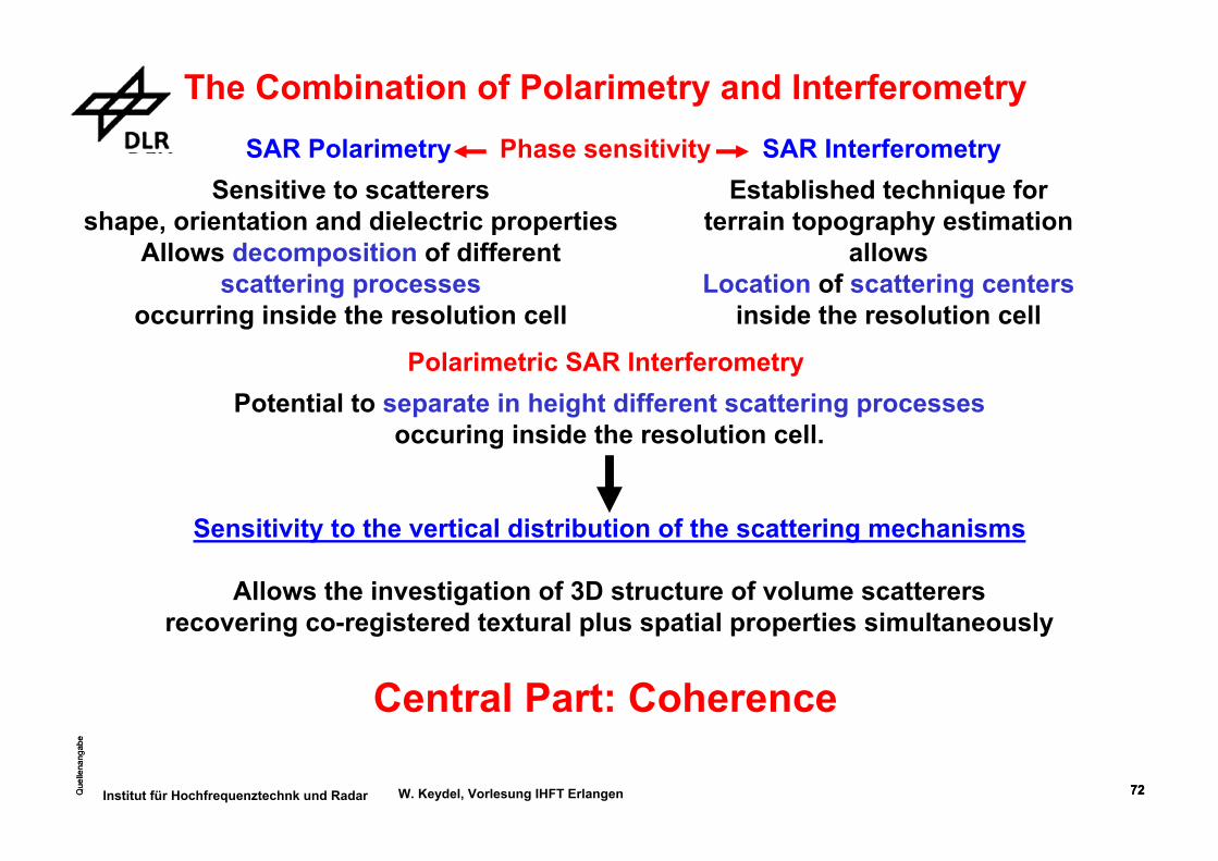
The Combination of Polarimetry and InterferometrySAR InterferometrySAR Polarimetry
Sensitive to scatterersshape, orientation and dielectric properties
Allows decomposition of different scattering processes
occurring inside the resolution cell
Established technique for terrain topography estimation
allows Location of scattering centers
inside the resolution cell
Polarimetric SAR InterferometryPotential to separate in height different scattering processes
occuring inside the resolution cell.
Sensitivity to the vertical distribution of the scattering mechanisms
Allows the investigation of 3D structure of volume scatterersrecovering co-registered textural plus spatial properties simultaneously
Phase sensitivity
Central Part: Coherence

Que
llena
ngab
e
73Que
llena
ngab
e
73Institut für Hochfrequenztechnk und Radar W. Keydel, Vorlesung IHFT Erlangen
Combination of Polarimetry and Interferometry
SAR Polarimetry (PolSAR) SAR Interferometry (InSAR)Allows decomposition of different
scattering processes inside resolution cell Allows location of the effective
scattering center inside resolution cell
Polarimetric SAR Interferometry (Pol-InSAR)
Potential to separate in height different scattering processes occurring inside the resolution cell.
Sensitivity to the vertical distribution of the scattering mechanisms
Allows the investigation of 3D structure of volume scatterers
InSAR DEMSAR ImagePauli Decomposition RGB
Que
llena
ngab
e
74Que
llena
ngab
e
74Institut für Hochfrequenztechnk und Radar W. Keydel, Vorlesung IHFT Erlangen
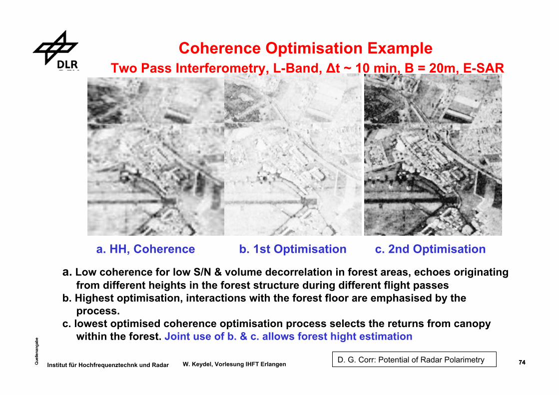
Coherence Optimisation ExampleTwo Pass Interferometry, L-Band, Δt ~ 10 min, B = 20m, E-SAR
a. HH, Coherence b. 1st Optimisation c. 2nd Optimisation
a. Low coherence for low S/N & volume decorrelation in forest areas, echoes originating from different heights in the forest structure during different flight passes
b. Highest optimisation, interactions with the forest floor are emphasised by the process.
c. lowest optimised coherence optimisation process selects the returns from canopywithin the forest. Joint use of b. & c. allows forest hight estimation
D. G. Corr: Potential of Radar Polarimetry
Que
llena
ngab
e
75Que
llena
ngab
e
75Institut für Hochfrequenztechnk und Radar W. Keydel, Vorlesung IHFT Erlangen
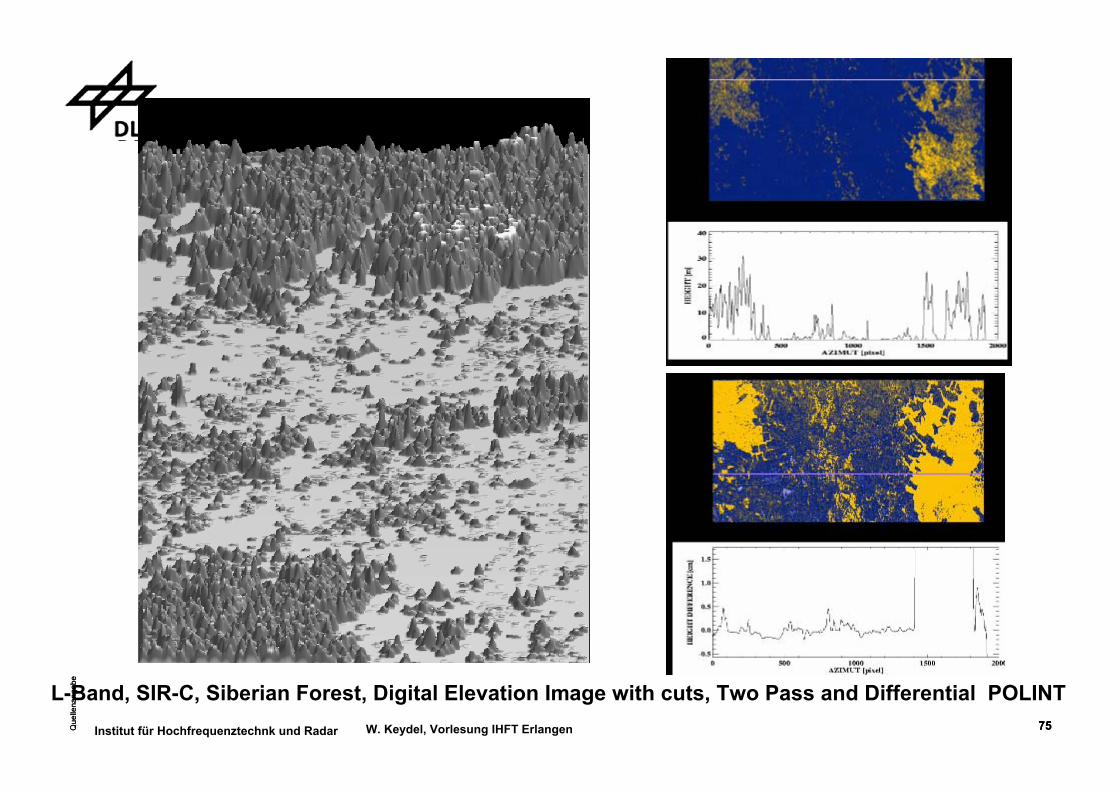
L-Band, SIR-C, Siberian Forest, Digital Elevation Image with cuts, Two Pass and Differential POLINT