Embed Size (px)
Citation preview
The Cryosphere, 12, 1433–1460, 2018https://doi.org/10.5194/tc-12-1433-2018© Author(s) 2018. This work is distributed underthe Creative Commons Attribution 4.0 License.
Design and results of the ice sheet model initialisation experimentsinitMIP-Greenland: an ISMIP6 intercomparisonHeiko Goelzer1,2, Sophie Nowicki3, Tamsin Edwards4,a, Matthew Beckley3, Ayako Abe-Ouchi5, Andy Aschwanden6,Reinhard Calov7, Olivier Gagliardini8, Fabien Gillet-Chaulet8, Nicholas R. Golledge9, Jonathan Gregory10,11,Ralf Greve12, Angelika Humbert13,14, Philippe Huybrechts15, Joseph H. Kennedy16,17, Eric Larour18,William H. Lipscomb19,20, Sébastien Le clec’h21, Victoria Lee22, Mathieu Morlighem23, Frank Pattyn2,Antony J. Payne22, Christian Rodehacke24,13, Martin Rückamp13, Fuyuki Saito25, Nicole Schlegel18,Helene Seroussi18, Andrew Shepherd26, Sainan Sun2, Roderik van de Wal1, and Florian A. Ziemen27
1Utrecht University, Institute for Marine and Atmospheric Research (IMAU), Utrecht, the Netherlands2Laboratoire de Glaciologie, Université Libre de Bruxelles, Brussels, Belgium3NASA GSFC, Cryospheric Sciences Branch, Greenbelt, USA4School of Environment, Earth & Ecosystem Sciences, The Open University, Milton Keynes, UK5Atmosphere Ocean Research Institute, University of Tokyo, Kashiwa, Japan6Geophysical Institute, University of Alaska Fairbanks, Fairbanks, USA7Potsdam Institute for Climate Impact Research, Potsdam, Germany8Univ. Grenoble Alpes, CNRS, IRD, Grenoble INP, IGE, 38000 Grenoble, France9Antarctic Research Centre, Victoria University of Wellington, Wellington, New Zealand10Department of Meteorology, University of Reading, Reading, UK11Met Office Hadley Centre, Exeter, UK12Institute of Low Temperature Science, Hokkaido University, Sapporo, Japan13Alfred Wegener Institute for Polar and Marine Research, Bremerhaven, Germany14University of Bremen, Bremen, Germany15Vrije Universiteit Brussel, Brussels, Belgium16Climate Change Science Institute, Oak Ridge National Laboratory, Oak Ridge, USA17Computational Sciences and Engineering Division, Oak Ridge National Laboratory, Oak Ridge, USA18Jet Propulsion Laboratory, California Institute of Technology, Pasadena, USA19Los Alamos National Laboratory, Los Alamos, USA20National Center for Atmospheric Research, Boulder, USA21LSCE/IPSL, Laboratoire des Sciences du Climat et de l’Environnement, CEA-CNRS-UVSQ, Gif-sur-Yvette, France22University of Bristol, Bristol, UK23University of California Irvine, Irvine, USA24Danish Meteorological Institute, Copenhagen, Denmark25Japan Agency for Marine-Earth Science and Technology, Yokohama, Japan26School of Earth and Environment, University of Leeds, Leeds, UK27Max Planck Institute for Meteorology, Hamburg, Germanyanow at: King’s College London, Department of Geography, London, UK
Correspondence: Heiko Goelzer ([email protected])
Received: 3 July 2017 – Discussion started: 14 July 2017Revised: 9 October 2017 – Accepted: 6 February 2018 – Published: 19 April 2018
Published by Copernicus Publications on behalf of the European Geosciences Union.
1434 H. Goelzer et al.: Design and results of the ice sheet model initialisation experiments
Abstract. Earlier large-scale Greenland ice sheet sea-levelprojections (e.g. those run during the ice2sea and SeaRISEinitiatives) have shown that ice sheet initial conditions havea large effect on the projections and give rise to importantuncertainties. The goal of this initMIP-Greenland intercom-parison exercise is to compare, evaluate, and improve the ini-tialisation techniques used in the ice sheet modelling commu-nity and to estimate the associated uncertainties in modelledmass changes. initMIP-Greenland is the first in a series of icesheet model intercomparison activities within ISMIP6 (theIce Sheet Model Intercomparison Project for CMIP6), whichis the primary activity within the Coupled Model Intercom-parison Project Phase 6 (CMIP6) focusing on the ice sheets.Two experiments for the large-scale Greenland ice sheet havebeen designed to allow intercomparison between participat-ing models of (1) the initial present-day state of the ice sheetand (2) the response in two idealised forward experiments.The forward experiments serve to evaluate the initialisationin terms of model drift (forward run without additional forc-ing) and in response to a large perturbation (prescribed sur-face mass balance anomaly); they should not be interpretedas sea-level projections. We present and discuss results thathighlight the diversity of data sets, boundary conditions, andinitialisation techniques used in the community to generateinitial states of the Greenland ice sheet. We find good agree-ment across the ensemble for the dynamic response to sur-face mass balance changes in areas where the simulated icesheets overlap but differences arising from the initial size ofthe ice sheet. The model drift in the control experiment is re-duced for models that participated in earlier intercomparisonexercises.
1 Introduction
Ice sheet model intercomparison exercises have a long his-tory, going back to the advent of large-scale ice sheet modelsin the early 1990s. The first intercomparison project (EIS-MINT, the European Ice Sheet Modelling INiTiative; Huy-brechts et al., 1996) defined three levels of possible com-parisons that could be distinguished. EISMINT and laterfollowing comparisons include (1) schematic experimentswith identical model setup and boundary conditions betweenmodels (e.g. Huybrechts et al., 1996; Pattyn et al., 2008,2012, 2013), (2) experiments allowing individual modellingdecisions (e.g. Payne et al., 2000; Calov et al., 2010; Asay-Davis et al., 2016), and (3) experiments of models appliedto real ice sheets (e.g. Shannon et al., 2013; Edwards et al.,2014b; Bindschadler et al., 2013; Nowicki et al., 2013a, b).In this genealogy, the present intercomparison is a type 3experiment with ice sheets models applied to simulate thelarge-scale present-day Greenland ice sheet (GrIS). The roleof this study is to assess the impact of initialisation on modelbehaviour; it is a precursor to ice sheet mass budget pro-
jections made using climate forcing for the atmosphere andocean. The initMIP-Greenland project is the first intercom-parison within ISMIP6, the Ice Sheet Model Intercompari-son Project for CMIP6 (Nowicki et al., 2016), which is theprimary activity within the Coupled Model IntercomparisonProject Phase 6 (CMIP6, Eyring et al., 2016) focusing on theice sheets. ISMIP6 is the first ice sheet model intercompari-son that is fully integrated within CMIP. This is an improve-ment to earlier initiatives like ice2sea (Gillet-Chaulet et al.,2012; Shannon et al., 2013; Goelzer et al., 2013; Edwards etal., 2014a, b) and SeaRISE (Sea-level Response to Ice SheetEvolution; Bindschadler et al., 2013; Nowicki et al., 2013a,b), which were lagging one iteration behind in terms of ap-plied climate forcing. More information on ISMIP6 can befound in the description paper (Nowicki et al., 2016) andon the Climate and Cryosphere (CliC)-hosted webpage (http://www.climate-cryosphere.org/activities/targeted/ismip6).
The initialisation of an ice sheet model forms the basisfor any prognostic model simulation and therefore revealsmost of the modelling decisions that distinguish different ap-proaches (Goelzer et al., 2017). It consists of defining boththe initial physical state of the ice sheet and model parame-ter values. In the context of initMIP-Greenland, we focus oninitialisation to the present day as a starting point for cen-tennial timescale future-sea-level-change projections (Now-icki et al., 2016). The need for physical ice flow models forsuch projections lies in the dynamic and highly non-linearresponse of ice sheet flow to changes in climatic forcing atthe atmospheric and oceanic boundaries. The surface massbalance (SMB) of the ice sheet is governed by the amount ofprecipitation falling on the surface and by meltwater runoffremoving mass predominantly at the margins. Mass is alsolost by melting at surfaces in contact with ocean water and bycalving of icebergs from marine-terminating outlet glaciers.Changes in ice sheet geometry generally cause changes inatmospheric conditions over the ice sheet and hence changesin SMB. An important effect is the height–SMB feedback,which causes decreasing SMB with decreasing ice surface el-evation and vice versa (e.g. Helsen et al., 2012; Franco et al.,2012; Edwards et al., 2014a; b). An important consequenceof the relation between SMB and ice flow is that negativeSMB removes ice before it can reach the marine marginsand thereby reduces the calving flux (e.g. Gillet-Chaulet etal., 2012; Goelzer et al., 2013; Fürst et al., 2015). An esti-mate for the recent balance of processes indicates that abla-tion (i.e. negative SMB) is responsible for two-thirds of theincreasing GrIS mass loss in the period 2009–2012, with icedischarge from marine-terminating outlet glaciers account-ing for the remaining third (Enderlin et al., 2014). While therelative importance of outlet glacier dynamics for total GrISmass loss has decreased since 2001 (Enderlin et al., 2014)and is expected to decrease further in the future (e.g. Goelzeret al., 2013; Fürst et al., 2015), it remains an important as-pect for projecting future sea-level contributions from the icesheet on the centennial timescale.
The Cryosphere, 12, 1433–1460, 2018 www.the-cryosphere.net/12/1433/2018/
H. Goelzer et al.: Design and results of the ice sheet model initialisation experiments 1435
Observations of ice sheet geometry and surface velocity,which ultimately form the target for any initialisation to thepresent-day state, have existed for only ∼ 25 years, i.e. onlysince the advent of the satellite era (e.g. Mouginot et al.,2015). This is a short period compared to the longer responsetimes of the ice sheet, which can be up to several thousandyears (Drewry et al., 1992), and makes it impossible to under-stand ice sheet changes based on observations alone. Whiledetailed observations mainly cover the ice surface properties,measurements for the ice interior and bed conditions are lim-ited to a handful of deep ice core drilling sites. Radar lay-ers dated at ice core sites can be used to extend the datingover large parts of the Greenland ice sheet (MacGregor et al.,2015), but this information is not well explored by ice sheetmodellers so far.
Projections of ice sheet response on decadal to centennialtimescales are strongly influenced by the initial state of theice sheet model (e.g. Arthern and Gudmundsson, 2010; Now-icki et al., 2013b; Adalgeirsdottir et al., 2014; Saito et al.,2016). The prognostic variables and parameters that need tobe defined for the initial state of an ice sheet model at thepresent day depend to some extent on the complexity of themodelling approach but typically consist of ice temperature(due to its impact on both ice rheology and basal slip), icesheet geometry, and boundary conditions at the base of theice sheet. For this time frame, ice sheet modellers face anissue similar to the one encountered in the weather/climatecommunity: whether to treat the problem as a “boundaryvalue problem” (climate prediction) or as an “initial-valueproblem” (weather forecasting).
Models developed for long-term and palaeoclimate simu-lations typically use “spin-up” procedures to determine theinitial state, where the ice sheet model is run forward intime for tens to hundreds of thousands of years with (chang-ing) reconstructed or modelled climatic boundary conditions(e.g. Huybrechts and de Wolde, 1999; Greve et al., 2011; As-chwanden et al., 2013). This implies that at any time duringthe simulation (except at the beginning where arbitrary con-ditions are set) the model’s state is defined as a consistent re-sponse to the forcing. Imperfections due to applied physicalapproximations, limited spatial resolution, and uncertainty inphysical parameters and climatic boundary conditions can re-sult in a considerable mismatch between the spun-up stateand present-day observations.
The main alternative to the spin-up approach is to use dataassimilation techniques, which leverage high-resolution ob-servations of geometry and velocity to initialise ice sheetmodels to the present-day state (e.g. Gillet-Chaulet et al.,2012; Seroussi et al., 2013; Arthern et al., 2015). They typ-ically infer poorly constrained basal conditions by a for-mal partial-differential-equations-constrained optimisationto match observed surface velocities for a given geometry(e.g. Morlighem et al., 2010). This implies that the inferredbasal parameters remain constant throughout the simulation,which is limited to the centennial timescale, where this is ap-
proximately the case. Data assimilation techniques producean initial state as consistent as possible with observationaldata but are affected by inconsistences (e.g. ice temperaturenot in equilibrium with the stress regime) and by uncertain-ties in observations (e.g. inconsistencies between differentobservational data sets; Seroussi et al., 2011). As data as-similations are designed to best fit observations, errors aris-ing from choices in ice parameters, from physical processes,from model resolution, from observational data sets, or fromignoring relevant state variables (e.g. ice rheology) are trans-ferred to basal conditions or other parameters obtained byinversion. An intermediate approach is assimilation of thegeometry of the ice sheet, by finding basal conditions that re-duce the mismatch with the observed ice sheet surface (Pol-lard and DeConto, 2012b). This method is typically appliedduring forward integration of the model and implies a modelstate in near balance with the forcing, though with a degree ofcompromise over matching observations. Note that the divi-sion of the different initialisation approaches presented hereis somewhat arbitrary. Combinations between different ap-proaches (e.g. relaxation after data assimilation) exist andneed to be further explored to improve initialisation tech-niques in the future.
Given the wide diversity of ice sheet initialisation tech-niques, the goal of initMIP-Greenland is to document, com-pare, and improve the techniques used by different groupsto initialise their state-of-the-art whole-ice-sheet models tothe present day as a starting point for centennial-timescalefuture-sea-level-change projections. A related goal is to high-light and understand how much of the spread in simulated icesheet evolution is related to the choices made in the initialisa-tion. All three methods currently used for initialisation of icesheet models (spin-up, assimilation of velocity, and assimi-lation of surface elevation) and variations thereof are repre-sented in our ensemble. We first describe our approach andexperimental setup in Sect. 2, and we present the participat-ing models in Sect. 3. Section 4 concentrates on the results,with the ice sheet model initial state explored in Sect. 4.1 andthe impact of initialisation on ice sheet evolutions analysedin Sect. 4.2. Discussion and conclusions follow in Sect. 5.
2 Approach and experimental setup
In initMIP-Greenland we focus on stand-alone ice sheetmodels, i.e. models not coupled to climate models. Althoughsome participating models have the capability to producetheir own SMB forcing, this is not a requirement in thepresent study. We have chosen to leave most of the modellingdecisions to the discretion of the participants, which servesto document the current state of the initialisation techniquesused in the ice sheet modelling community. Conversely, thisimplies a relatively heterogeneous ensemble with only inci-dental overlap of modelling choices between different sub-missions.
www.the-cryosphere.net/12/1433/2018/ The Cryosphere, 12, 1433–1460, 2018
1436 H. Goelzer et al.: Design and results of the ice sheet model initialisation experiments
Table 1. Summary of the ISMIP6 initMIP-Greenland experiments (n/a: not applicable).
Experiment title Experiment label CMIP6 Label (experiment_id) Experiment description Duration of the simulation Major purposes
Initialisation init ism–init–std Initialisation to present day n/a EvaluationControl ctrl ism–ctrl–std Unforced control experiment 100 yr EvaluationSMB anomaly asmb ism–asmb–std Idealised change in SMB forcing 100 yr Evaluation
Experiments for the large-scale Greenland ice sheet havebeen designed to allow intercomparison of the modelled ini-tial present-day states and of the model responses to a largeperturbation in SMB forcing (Table 1). Modellers were askedto initialise their model to the present day with the methodof their choice (init) and then run two forward experimentsto evaluate the initialisation in terms of model drift: a con-trol run without any change in the forcing (ctrl) and a per-turbed run with a large prescribed surface mass balanceanomaly (asmb). The prescribed SMB anomaly in experi-ment asmb (Appendix A) implies a strongly negative SMBforcing, in line with what may be expected from upper-endclimate change scenarios. Nevertheless, the sea-level contri-bution from these experiments should not be interpreted as aprojection, but rather as a diagnostic to evaluate model dif-ferences.
Note that the time of initialisation was not strictly defined(in the range 1950–2016), as modellers assign different datesto their initial state according to the data sets used. The par-ticipants were also largely free in other modelling decisions,with only the imposed constraint for the forward experimentsthat all boundary conditions and forcing remain constant intime. In particular, the SMB is not allowed to change (e.g.with surface elevation) other than by the prescribed SMBanomaly. All information and documentation concerning theISMIP6 initMIP-Greenland experiments can be found onthe ISMIP6 wiki (http://www.climate-cryosphere.org/wiki/index.php?title=InitMIP-Greenland).
While modellers were free to use a native model grid oftheir choice, model output was submitted on a common gridto support a consistent analysis (see Appendix C). This im-plies that results had to first be interpolated from the na-tive model grid to the output grid, which for state variableshas in most cases been done using conservative interpolation(Jones, 1999). In the following we present all results on theoutput grid with a horizontal resolution of 5×5 km. Further-more, all ice sheet results have been masked to exclude iceon Ellesmere Island and Iceland.
3 Participating groups and models
Participants in initMIP-Greenland from 17 groups and col-laborations (Table 2) have provided 35 model submissions.There is some overlap between the code bases used by dif-ferent groups, with ultimately 11 individual ice flow mod-els. However, the same model used by different groups (with
varying data sets and initialisation procedures) may lead torather different results. These submissions cover a wide spec-trum of model resolutions, applied physical approximations,boundary conditions, and initialisation techniques, whichmakes for a heterogeneous ensemble. In some cases, thesame group has used two or more different model versionsor different initialisation techniques, with several groups run-ning their models at varying horizontal grid resolution. Inthe following we will refer to each separate submission as a“model”, identified by the model ID in the table of generalmodel characteristics (Table 3). A detailed description of theindividual models and initialisation techniques can be foundin Appendix B.
Despite the diversity in modelling approaches (Table 3)and the overlap between different methods, it is useful to dis-tinguish the three main classes of initialisation techniques de-scribed before: first, those using a form of data assimilation(DA) to match observed velocities (DAv); second, those thatrely solely on model spin-up (SP); and third, the intermedi-ate case of transient assimilation to match surface elevation(DAs). However, even DAv is typically preceded by someform of spin-up (with the same model or a different one)to produce the internal temperature of the ice sheet, and itmay also be followed by a relaxation run to make the veloci-ties and geometry more consistent. The represented cases ofDA infer a spatially varying basal drag coefficient to min-imise the mismatch with observations of velocity or geome-try. Models using SP use physical parameters and processesto define the basal conditions.
Modelling choices also differ based on model purpose andtypical application. Many of the SP models have been builtand used for palaeo-applications for time periods when pos-sible DA targets are very limited and SMB boundary con-ditions differ from the present. This makes it necessary inthose models to parameterise SMB, for example by usingpositive-degree-day (PDD) models (e.g. Huybrechts et al.,1991). SP approaches are also generally favoured when in-cluding ice sheets in coupled climate models. In two groups(DMI, MPIM), the ice sheet models and SMB forcing are setup in a similar way to how they would be for coupled icesheet–climate simulations. In contrast, the DAv models arebuilt specifically for centennial timescale future projections,while DAs again represents an intermediate case of modelstypically used for long-term simulations but specifically ini-tialised for the present day. These fundamental differences inmodelling approaches have to be kept in mind when com-paring the models. The SMB is in many cases taken from
The Cryosphere, 12, 1433–1460, 2018 www.the-cryosphere.net/12/1433/2018/
H. Goelzer et al.: Design and results of the ice sheet model initialisation experiments 1437
Table 2. Participants, ice sheet models, and modelling groups in ISMIP6 initMIP-Greenland.
Contributors Model Group ID Group
Victoria Lee,Stephen L. Cornford,Antony J. Payne,Daniel F. Martin
BISICLES BGC Centre for Polar Observation and Modelling, School of GeographicalSciences, University of Bristol, Bristol, UK; Department of Geogra-phy, College of Science, Swansea University, Swansea, UK; Compu-tational Research Division, Lawrence Berkeley National Laboratory,Berkeley, California, USA
William H. Lipscomb,Joseph H. Kennedy
CISM LANL Los Alamos National Laboratory, Los Alamos, USA; National Centerfor Atmospheric Research, Boulder, USA; Climate Change ScienceInstitute, Oak Ridge National Laboratory, Oak Ridge, USA; Compu-tational Sciences and Engineering Division, Oak Ridge National Lab-oratory, Oak Ridge, USA
Fabien Gillet-Chaulet,Olivier Gagliardini
Elmer IGE Institut des Géosciences de L’Environnement, Univ. Grenoble Alpes,CNRS, IRD, Grenoble INP, IGE, 38000 Grenoble, FR
Sainan Sun,Frank Pattyn
FETISH ULB Laboratoire de Glaciologie, Université Libre de Bruxelles, Brussels,BE
Philippe Huybrechts,Heiko Goelzer
GISM VUB Vrije Universiteit Brussel, Brussels, BE
Sébastien Le clec’h GRISLI LSCE LSCE/IPSL, Laboratoire des Sciences du Climat et del’Environnement, CEA-CNRS-UVSQ, Gif-sur-Yvette, FR
Fuyuki Saito,Ayako Abe-Ouchi
IcIES MIROC Japan Agency for Marine-Earth Science and Technology, JP; The Uni-versity of Tokyo, Tokyo, JP
Heiko Goelzer,Roderik van de Wal
IMAUICE IMAU Utrecht University, Institute for Marine and Atmospheric Research(IMAU), Utrecht, NL
Helene Seroussi,Nicole Schlegel
ISSM JPL Caltech’s Jet Propulsion Laboratory, Pasadena, USA
Helene Seroussi,Mathieu Morlighem
ISSM UCI_JPL Caltech’s Jet Propulsion Laboratory, Pasadena, USA;University of California Irvine, USA
Martin Rückamp,Angelika Humbert
ISSM AWI Alfred Wegener Institute for Polar and Marine Research, DE; Univer-sity of Bremen, DE
Andy Aschwanden PISM UAF Geophysical Institute, University of Alaska Fairbanks, USA
Nicholas R. Golledge PISM ARC Antarctic Research Centre, Victoria University of Wellington, NZ
Christian Rodehacke PISM DMI Danish Meteorological Institute, DK; Alfred Wegener Institute for Po-lar and Marine Research, DE
Florian A. Ziemen PISM MPIM Max Planck Institute for Meteorology, DE
Ralf Greve SICOPOLIS ILTS Institute of Low Temperature Science, Hokkaido University, Sapporo,JP
Ralf Greve,Reinhard Calov
SICOPOLIS ILTS_ PIK Institute of Low Temperature Science, Hokkaido University, Sapporo,JP; Potsdam Institute for Climate Impact Research, Potsdam, DE
regional climate model (RCM) simulations, but it arises insome cases from parameterisations based on the modelledice sheet geometry applying traditional PDD methods.
4 Results
In this section, we first present results of the init experiment,designed to compare the present-day initial state betweenparticipating models and against observations. These or sim-ilar initial model states would serve as a starting point forphysically based projections of the Greenland ice sheet con-
www.the-cryosphere.net/12/1433/2018/ The Cryosphere, 12, 1433–1460, 2018
1438 H. Goelzer et al.: Design and results of the ice sheet model initialisation experiments
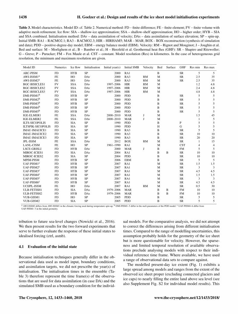
Table 3. Model characteristics. Model ID: cf. Table 2. Numerical method: FD – finite difference; FE – finite element; FV – finite volume withadaptive mesh refinement. Ice flow: SIA – shallow-ice approximation; SSA – shallow-shelf approximation; HO – higher order; HYB – SIAand SSA combined. Initialisation method: DAv – data assimilation of velocity; DAs – data assimilation of surface elevation; SP – spin-up.Initial SMB: RA1 – RACMO2.1; RA3 – RACMO2.3; HIR – HIRHAM5; MAR – MAR; BOX – BOX reconstruction (synthesis of simulationand data); PDD – positive-degree-day model; EBM – energy balance model (EBM). Velocity: RM – Rignot and Mouginot; J – Joughin et al.Bed and surface: M – Morlighem et al.; B – Bamber et al.; H – Herzfeld et al. Geothermal heat flux (GHF): SR – Shapiro and Ritzwoller;G – Greve; P – Purucker; FM – Fox Maule et al. CST – constant. Model resolution (Res) in kilometres. In the case of heterogeneous gridresolution, the minimum and maximum resolution are given.
Model ID Numerics Ice flow Initialisation Initial year(s) Initial SMB Velocity Bed Surface GHF Res min Res max
ARC-PISM FD HYB SP 2000 RA1 B SR 5 5AWI-ISSM1a FE HO DAv 2000 RA3 RM M SR 2.5 35AWI-ISSM2a FE HO DAv 2000 RA3 RM M SR 2.5 35BGC-BISICLES1 FV SSA DAv 1997–2006 HIR RM M 1.2 4.8BGC-BISICLES2 FV SSA DAv 1997–2006 HIR RM M 2.4 4.8BGC-BISICLES3 FV SSA DAv 1997–2006 HIR RM M 4.8 4.8DMI-PISM1b FD HYB SP 2000 PDD B SR 5 5DMI-PISM2b FD HYB SP 2000 PDD B SR 5 5DMI-PISM3b FD HYB SP 2000 PDD B SR 5 5DMI-PISM4b FD HYB SP 2000 PDD B SR 5 5DMI-PISM5b FD HYB SP 2000 PDD B SR 5 5IGE-ELMER1 FE SSA DAv 2000–2010 MAR J M 1.5 45IGE-ELMER2 FE SSA DAv 2000–2010 MAR J M 1 5ILTS-SICOPOLIS FD SIA SP 1990 PDD B P 5 5ILTSPIK-SICOPOLIS FD SIA SP 1990 PDD H G 5 5IMAU-IMAUICE1 FD SIA SP 1990 RA3 B SR 5 5IMAU-IMAUICE2 FD SIA SP 1990 RA3 B SR 10 10IMAU-IMAUICE3 FD SIA SP 1990 RA3 B SR 20 20JPL-ISSM FE SSA DAv 2012 BOX RM M SR 1 15LANL-CISM FE HO SP 1961–1990 RA1 M CST 4 4LSCE-GRISLI FD HYB DAv 2000 MAR J B FM 5 5MIROC-ICIES1 FD SIA DAs 2004 RA1 B B SR 10 10MIROC-ICIES2 FD SIA SP 2004 PDD B SR 10 10MPIM-PISM FD HYB SP 2006 EBM B SR 5 5UAF-PISM1c FD HYB SP 2007 RA1 M SR 1.5 1.5UAF-PISM2c FD HYB SP 2007 RA1 M SR 3 3UAF-PISM3c FD HYB SP 2007 RA1 M SR 4.5 4.5UAF-PISM4c FD HYB SP 2007 RA1 M SR 1.5 1.5UAF-PISM5c FD HYB SP 2007 RA1 M SR 3 3UAF-PISM6c FD HYB SP 2007 RA1 M SR 4.5 4.5UCIJPL-ISSM FE HO DAv 2007 RA1 RM M SR 0.5 30ULB-FETISH1 FD SIA DAs 1979–2006 MAR B B FM 10 10ULB-FETISH2 FD HYB DAs 1979–2006 MAR B B FM 10 10VUB-GISM1 FD HO SP 2005 PDD B SR 5 5VUB-GISM2 FD SIA SP 2005 PDD B SR 5 5
a AWI-ISSM2 differs from AWI-ISSM1 in the climatic forcing used during temperature spin-up. b DMI-PISM1–5 differ in the melt parameters of the PDD model. c UAF-PISM4–6 differ fromUAF-PISM1–3 in the initial geometry.
tribution to future sea-level changes (Nowicki et al., 2016).We then present results for the two forward experiments thatserve to further evaluate the response of these initial states toidealised forcing (ctrl, asmb).
4.1 Evaluation of the initial state
Because initialisation techniques generally differ in the ob-servational data used as model input, boundary conditions,and assimilation targets, we did not prescribe the year(s) ofinitialisation. The initialisation times in the ensemble (Ta-ble 3) therefore represent the time frame(s) of the observa-tions that are used for data assimilation (in case DA) and thesimulated SMB used as a boundary condition for the individ-
ual models. For the comparative analysis, we did not attemptto correct the differences arising from different initialisationtimes. Compared to the range of modelling uncertainties, thisassumption probably holds for the geometry of the ice sheetbut is more questionable for velocity. However, the sparse-ness and limited temporal resolution of available observa-tions preclude analysing models with respect to their indi-vidual reference time frame. Where available, we have useda range of observational data sets to compare against.
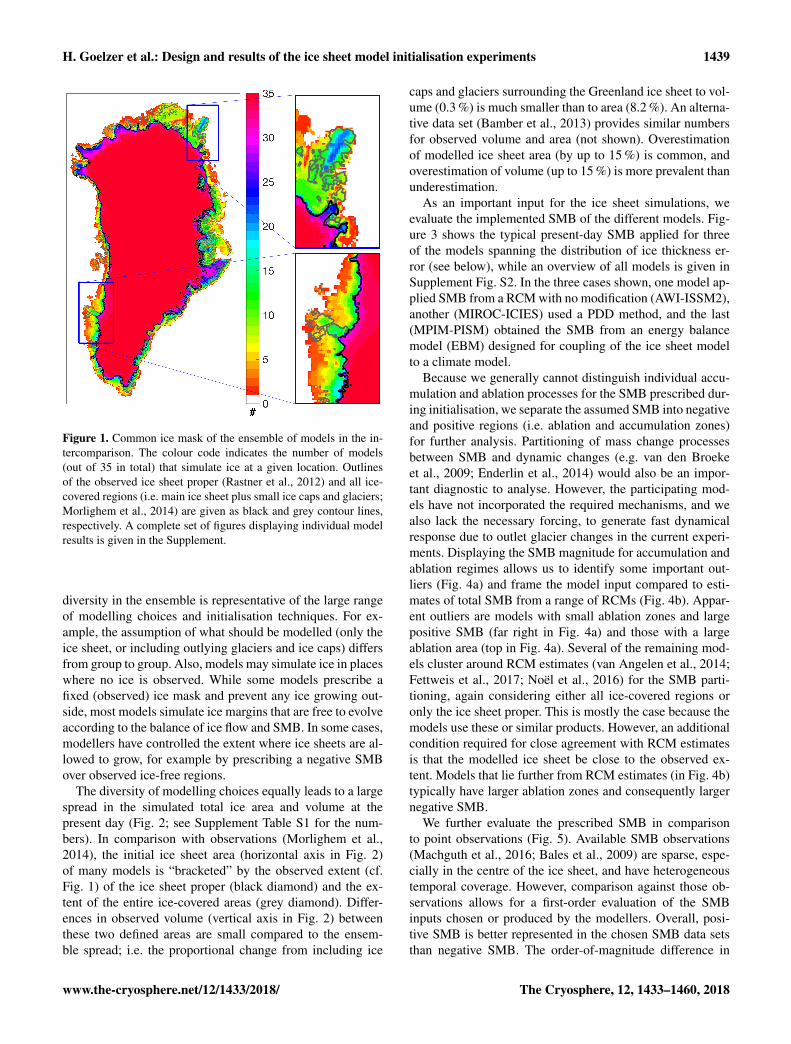
The modelled present-day ice extent (Fig. 1) exhibits alarge spread among models and ranges from the extent of theobserved ice sheet proper (excluding connected glaciers andice caps) to nearly filling the entire land above sea level (seealso Supplement Fig. S2 for individual model results). This
The Cryosphere, 12, 1433–1460, 2018 www.the-cryosphere.net/12/1433/2018/
H. Goelzer et al.: Design and results of the ice sheet model initialisation experiments 1439
Figure 1. Common ice mask of the ensemble of models in the in-tercomparison. The colour code indicates the number of models(out of 35 in total) that simulate ice at a given location. Outlinesof the observed ice sheet proper (Rastner et al., 2012) and all ice-covered regions (i.e. main ice sheet plus small ice caps and glaciers;Morlighem et al., 2014) are given as black and grey contour lines,respectively. A complete set of figures displaying individual modelresults is given in the Supplement.
diversity in the ensemble is representative of the large rangeof modelling choices and initialisation techniques. For ex-ample, the assumption of what should be modelled (only theice sheet, or including outlying glaciers and ice caps) differsfrom group to group. Also, models may simulate ice in placeswhere no ice is observed. While some models prescribe afixed (observed) ice mask and prevent any ice growing out-side, most models simulate ice margins that are free to evolveaccording to the balance of ice flow and SMB. In some cases,modellers have controlled the extent where ice sheets are al-lowed to grow, for example by prescribing a negative SMBover observed ice-free regions.
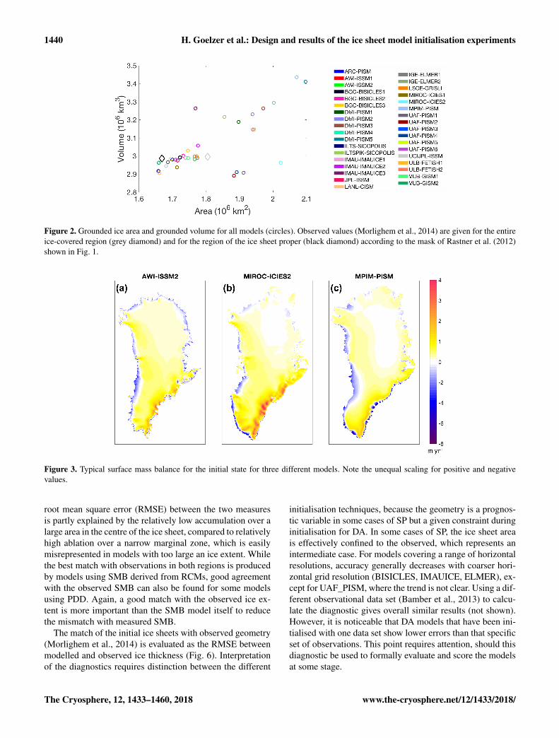
The diversity of modelling choices equally leads to a largespread in the simulated total ice area and volume at thepresent day (Fig. 2; see Supplement Table S1 for the num-bers). In comparison with observations (Morlighem et al.,2014), the initial ice sheet area (horizontal axis in Fig. 2)of many models is “bracketed” by the observed extent (cf.Fig. 1) of the ice sheet proper (black diamond) and the ex-tent of the entire ice-covered areas (grey diamond). Differ-ences in observed volume (vertical axis in Fig. 2) betweenthese two defined areas are small compared to the ensem-ble spread; i.e. the proportional change from including ice
caps and glaciers surrounding the Greenland ice sheet to vol-ume (0.3 %) is much smaller than to area (8.2 %). An alterna-tive data set (Bamber et al., 2013) provides similar numbersfor observed volume and area (not shown). Overestimationof modelled ice sheet area (by up to 15 %) is common, andoverestimation of volume (up to 15 %) is more prevalent thanunderestimation.
As an important input for the ice sheet simulations, weevaluate the implemented SMB of the different models. Fig-ure 3 shows the typical present-day SMB applied for threeof the models spanning the distribution of ice thickness er-ror (see below), while an overview of all models is given inSupplement Fig. S2. In the three cases shown, one model ap-plied SMB from a RCM with no modification (AWI-ISSM2),another (MIROC-ICIES) used a PDD method, and the last(MPIM-PISM) obtained the SMB from an energy balancemodel (EBM) designed for coupling of the ice sheet modelto a climate model.
Because we generally cannot distinguish individual accu-mulation and ablation processes for the SMB prescribed dur-ing initialisation, we separate the assumed SMB into negativeand positive regions (i.e. ablation and accumulation zones)for further analysis. Partitioning of mass change processesbetween SMB and dynamic changes (e.g. van den Broekeet al., 2009; Enderlin et al., 2014) would also be an impor-tant diagnostic to analyse. However, the participating mod-els have not incorporated the required mechanisms, and wealso lack the necessary forcing, to generate fast dynamicalresponse due to outlet glacier changes in the current experi-ments. Displaying the SMB magnitude for accumulation andablation regimes allows us to identify some important out-liers (Fig. 4a) and frame the model input compared to esti-mates of total SMB from a range of RCMs (Fig. 4b). Appar-ent outliers are models with small ablation zones and largepositive SMB (far right in Fig. 4a) and those with a largeablation area (top in Fig. 4a). Several of the remaining mod-els cluster around RCM estimates (van Angelen et al., 2014;Fettweis et al., 2017; Noël et al., 2016) for the SMB parti-tioning, again considering either all ice-covered regions oronly the ice sheet proper. This is mostly the case because themodels use these or similar products. However, an additionalcondition required for close agreement with RCM estimatesis that the modelled ice sheet be close to the observed ex-tent. Models that lie further from RCM estimates (in Fig. 4b)typically have larger ablation zones and consequently largernegative SMB.
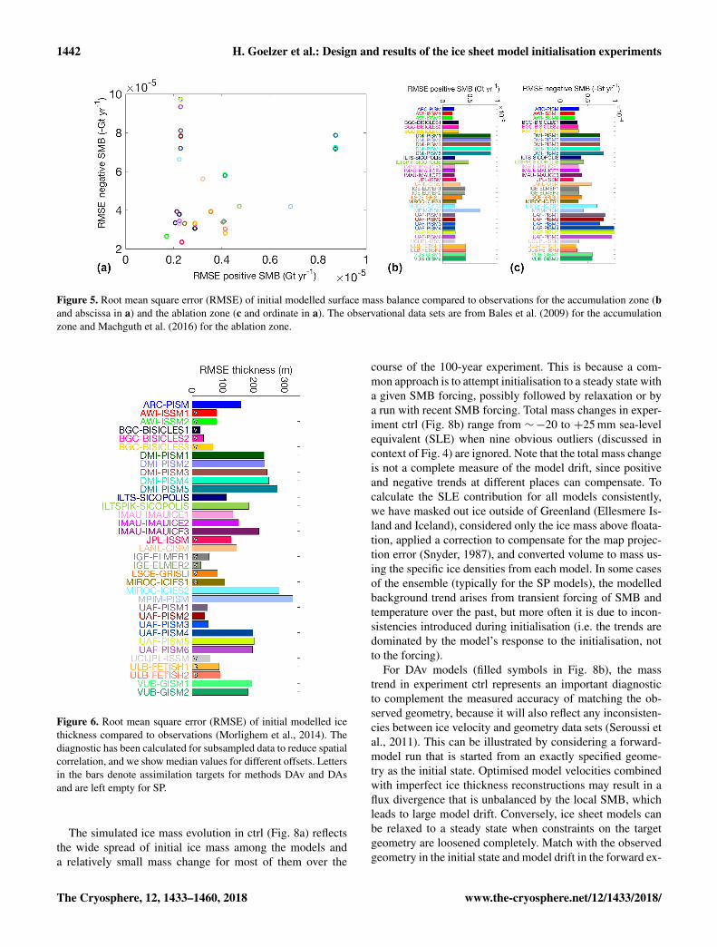
We further evaluate the prescribed SMB in comparisonto point observations (Fig. 5). Available SMB observations(Machguth et al., 2016; Bales et al., 2009) are sparse, espe-cially in the centre of the ice sheet, and have heterogeneoustemporal coverage. However, comparison against those ob-servations allows for a first-order evaluation of the SMBinputs chosen or produced by the modellers. Overall, posi-tive SMB is better represented in the chosen SMB data setsthan negative SMB. The order-of-magnitude difference in
www.the-cryosphere.net/12/1433/2018/ The Cryosphere, 12, 1433–1460, 2018
1440 H. Goelzer et al.: Design and results of the ice sheet model initialisation experiments
Figure 2. Grounded ice area and grounded volume for all models (circles). Observed values (Morlighem et al., 2014) are given for the entireice-covered region (grey diamond) and for the region of the ice sheet proper (black diamond) according to the mask of Rastner et al. (2012)shown in Fig. 1.
Figure 3. Typical surface mass balance for the initial state for three different models. Note the unequal scaling for positive and negativevalues.
root mean square error (RMSE) between the two measuresis partly explained by the relatively low accumulation over alarge area in the centre of the ice sheet, compared to relativelyhigh ablation over a narrow marginal zone, which is easilymisrepresented in models with too large an ice extent. Whilethe best match with observations in both regions is producedby models using SMB derived from RCMs, good agreementwith the observed SMB can also be found for some modelsusing PDD. Again, a good match with the observed ice ex-tent is more important than the SMB model itself to reducethe mismatch with measured SMB.
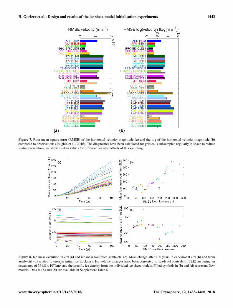
The match of the initial ice sheets with observed geometry(Morlighem et al., 2014) is evaluated as the RMSE betweenmodelled and observed ice thickness (Fig. 6). Interpretationof the diagnostics requires distinction between the different
initialisation techniques, because the geometry is a prognos-tic variable in some cases of SP but a given constraint duringinitialisation for DA. In some cases of SP, the ice sheet areais effectively confined to the observed, which represents anintermediate case. For models covering a range of horizontalresolutions, accuracy generally decreases with coarser hori-zontal grid resolution (BISICLES, IMAUICE, ELMER), ex-cept for UAF_PISM, where the trend is not clear. Using a dif-ferent observational data set (Bamber et al., 2013) to calcu-late the diagnostic gives overall similar results (not shown).However, it is noticeable that DA models that have been ini-tialised with one data set show lower errors than that specificset of observations. This point requires attention, should thisdiagnostic be used to formally evaluate and score the modelsat some stage.
The Cryosphere, 12, 1433–1460, 2018 www.the-cryosphere.net/12/1433/2018/

H. Goelzer et al.: Design and results of the ice sheet model initialisation experiments 1441
Figure 4. Negative and positive SMB of all models (a) and for themarked inset excluding outliers (b). Diamonds, squares, and tri-angles in (b) give partitioning from average 1979–2000 regionalclimate model simulations (van Angelen et al., 2014; Fettweis etal., 2017; Noël et al., 2016) with masking to the ice-covered re-gion (grey) and to the ice sheet proper (IS, black) according to themask of Rastner et al. (2012). Compare symbol colour to identifyindividual models with Figs. 3–5. Data are available in SupplementTable S1.
To evaluate the match of the models with observed sur-face ice velocities, we have computed the RMSE between themodelled and observed (Joughin et al., 2016) velocity mag-nitude (Fig. 7a). Calculating the RMSE based on the log ofthe velocities instead (Fig. 7b) results in a slightly differentpicture, because errors in high velocities typically occurringat the margins over a relatively small fraction of the ice sheetarea are weighted less. We note that an alternative choice ofmetric would be one that accounts for spatial variation in ob-servational uncertainty, such as standardised Euclidean dis-tance. Distinction between models using DAv and the rest isagain useful, since velocity is not an independent variable incases where it enters the inversion calculations. Models us-ing observed velocities in the DAv procedure could in prin-ciple be compared with each other to evaluate the successof the inversion technique. However, the comparison wouldhave to take into account that some groups use relaxation af-ter the DAv step to get a better consistency between the icegeometry and velocity. This modifies the results dependingon the relaxation time. Better consistency for a model canbe achieved with longer relaxation time, at the expense of a
larger discrepancy with the observed geometry. In any case,not every group uses the same velocity data set (e.g. Rignotand Mouginot, 2012; Joughin et al., 2016).
It is interesting to note that DAs techniques using onlysurface elevation as an inversion target can have quite lowerrors in simulated velocities, which implies an overall con-sistency between geometry and velocity structure of the mod-elled ice sheets. Although this consistency is expected basedon mass conservation, the results confirm that the basic as-sumptions (e.g. approximation to the force balance and rhe-ology structure) are generally close enough to reality. This isparticularly important considering that DAv techniques canmatch observed velocities well for almost any given rheol-ogy, as all the uncertainty (including unknown rheology) iscompounded in the basal sliding relation.
4.2 Results of the forward experiments
The two experiments ctrl and asmb have been performed tofurther test the modelled initial states in terms of their be-haviour in typical forward simulations. This is needed toexpose model response to changing constraints that werepresent during initialisation. Furthermore, we evaluate the in-fluence of the initial state and of modelling decisions pertain-ing to the initialisation on the results of the forward experi-ments, i.e. the projected ice thickness change and sea-levelcontribution.
The experiment ctrl serves to evaluate the model responsein the absence of additional forcing and is an important stepto understand the consequence of modelling choices for for-ward experiments. Since we have not specified any assump-tion on the imbalance between SMB and ice flow at the initialstate, the ice sheet would ideally exhibit an imbalance thatmatches observations for a given time interval. Recent mod-elled mass trends or thickness changes could then in principlebe evaluated with existing observational data sets of limitedtime coverage (e.g. Velicogna et al., 2014). Reproducing re-cent changes seen by GRACE (mass change) and altimetry(thickness change), however, is hampered by not knowingthe ice sheet bedrock and surface elevation well at the timethat the satellite started to observe and would also assess theaccuracy of the SMB input (i.e. for many models, a sepa-rate RCM). Furthermore, this would require that the experi-ments aimed for realistic outlet glacier dynamics and oceanforcing (e.g. Nick et al., 2013), which are currently not avail-able (Alexander et al., 2016; Schlegel et al., 2016) and havedeliberately not been included in the present experiments.Approaches to validate models using hindcasting techniques(Aschwanden et al., 2013; Larour et al., 2014, 2016; Priceet al., 2017) currently suffer the same limitations of obser-vational data sets with short time coverage, uncertainty inexternal forcing, limited knowledge of processes responsi-ble for dynamic outlet glacier response, and the initialisationproblems discussed above.
www.the-cryosphere.net/12/1433/2018/ The Cryosphere, 12, 1433–1460, 2018
1442 H. Goelzer et al.: Design and results of the ice sheet model initialisation experiments
Figure 5. Root mean square error (RMSE) of initial modelled surface mass balance compared to observations for the accumulation zone (band abscissa in a) and the ablation zone (c and ordinate in a). The observational data sets are from Bales et al. (2009) for the accumulationzone and Machguth et al. (2016) for the ablation zone.
Figure 6. Root mean square error (RMSE) of initial modelled icethickness compared to observations (Morlighem et al., 2014). Thediagnostic has been calculated for subsampled data to reduce spatialcorrelation, and we show median values for different offsets. Lettersin the bars denote assimilation targets for methods DAv and DAsand are left empty for SP.
The simulated ice mass evolution in ctrl (Fig. 8a) reflectsthe wide spread of initial ice mass among the models anda relatively small mass change for most of them over the
course of the 100-year experiment. This is because a com-mon approach is to attempt initialisation to a steady state witha given SMB forcing, possibly followed by relaxation or bya run with recent SMB forcing. Total mass changes in exper-iment ctrl (Fig. 8b) range from ∼−20 to +25 mm sea-levelequivalent (SLE) when nine obvious outliers (discussed incontext of Fig. 4) are ignored. Note that the total mass changeis not a complete measure of the model drift, since positiveand negative trends at different places can compensate. Tocalculate the SLE contribution for all models consistently,we have masked out ice outside of Greenland (Ellesmere Is-land and Iceland), considered only the ice mass above floata-tion, applied a correction to compensate for the map projec-tion error (Snyder, 1987), and converted volume to mass us-ing the specific ice densities from each model. In some casesof the ensemble (typically for the SP models), the modelledbackground trend arises from transient forcing of SMB andtemperature over the past, but more often it is due to incon-sistencies introduced during initialisation (i.e. the trends aredominated by the model’s response to the initialisation, notto the forcing).
For DAv models (filled symbols in Fig. 8b), the masstrend in experiment ctrl represents an important diagnosticto complement the measured accuracy of matching the ob-served geometry, because it will also reflect any inconsisten-cies between ice velocity and geometry data sets (Seroussi etal., 2011). This can be illustrated by considering a forward-model run that is started from an exactly specified geome-try as the initial state. Optimised model velocities combinedwith imperfect ice thickness reconstructions may result in aflux divergence that is unbalanced by the local SMB, whichleads to large model drift. Conversely, ice sheet models canbe relaxed to a steady state when constraints on the targetgeometry are loosened completely. Match with the observedgeometry in the initial state and model drift in the forward ex-
The Cryosphere, 12, 1433–1460, 2018 www.the-cryosphere.net/12/1433/2018/
H. Goelzer et al.: Design and results of the ice sheet model initialisation experiments 1443
Figure 7. Root mean square error (RMSE) of the horizontal velocity magnitude (a) and the log of the horizontal velocity magnitude (b)compared to observations (Joughin et al., 2016). The diagnostics have been calculated for grid cells subsampled regularly in space to reducespatial correlation; we show median values for different possible offsets of this sampling.
Figure 8. Ice mass evolution in ctrl (a) and ice mass loss from asmb–ctrl (c). Mass change after 100 years in experiment ctrl (b) and fromasmb–ctrl (d) related to error in initial ice thickness. Ice volume changes have been converted to sea-level equivalent (SLE) assuming anocean area of 361.8×10⁶ km2 and the specific ice density from the individual ice sheet models. Filled symbols in (b) and (d) represent DAvmodels. Data in (b) and (d) are available in Supplement Table S1.
www.the-cryosphere.net/12/1433/2018/ The Cryosphere, 12, 1433–1460, 2018
1444 H. Goelzer et al.: Design and results of the ice sheet model initialisation experiments
Figure 9. Typical surface mass balance after 100 years in experiment asmb for the three models in Fig. 3. Note the unequal scaling forpositive and negative values.
periment are therefore complementary measures that shouldbe considered together. While this is evident for any singlemodel, we only find tentative confirmation amongst the DAvmodels in our ensemble (filled symbols in Fig. 8b), with in-creasing mass trend for decreasing ice thickness error.
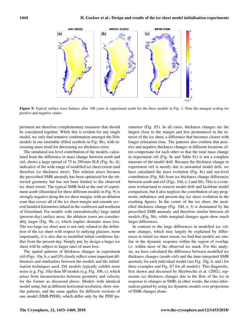
The simulated sea-level contribution of the models, calcu-lated from the difference in mass change between asmb andctrl, shows a large spread of 75 to 290 mm SLE (Fig. 8c, d),indicative of the wide range of modelled ice sheet extent (andtherefore ice thickness error). This relation arises becausethe prescribed SMB anomaly has been optimised for the ob-served geometry but has not been limited to the observedice sheet extent. The typical SMB field at the end of experi-ment asmb (illustrated for three different models in Fig. 9) isstrongly negative along the ice sheet margin, with an ablationzone that covers all of the ice sheet margin and extends sev-eral hundred kilometres inland in the southwest and northeastof Greenland. For models with (unrealistically) large initial(present-day) surface areas, the ablation zones are consider-ably larger (Fig. 9b, c), which implies dramatic mass loss.The too-large ice sheet area is not only related to the defini-tion of the ice sheet with respect to outlying glaciers; moreimportantly, it is also due to modelled initial conditions fur-ther from the present day. Simply put, by design a larger icesheet will be subject to larger rates of mass loss.
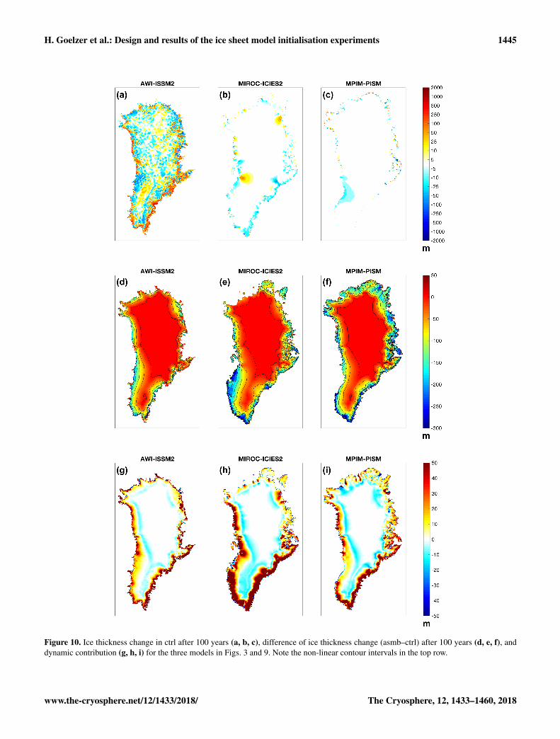
The spatial patterns of thickness changes in experimentctrl (Figs. 10a, b, c and S5) clearly reflect some important dif-ferences and similarities between the models and the initial-isation techniques used. DA models typically exhibit morenoise (e.g. Fig. 10a) than SP models (e.g. Fig. 10b, c), whicharises from inconsistencies between geometry and velocityfor the former as discussed above. Models with identicalmodel setup, but at different horizontal resolution, show sim-ilar patterns, and the same applies for different versions ofone model (DMI-PISM), which differ only by the PDD pa-
rameters (Fig. S5). In all cases, thickness changes are thelargest close to the margin and less pronounced in the in-terior of the ice sheet, a difference that becomes clearer withlonger relaxation time. The patterns also confirm that posi-tive and negative thickness changes at different locations of-ten compensate for each other so that the total mass changein experiment ctrl (Fig. 8c and Table S1) is not a completemeasure of the model drift. Because the thickness change inexperiment ctrl is mostly due to unwanted model drift, wehave calculated the mass evolution (Fig. 8c) and sea-levelcontribution (Fig. 8d) from ice thickness change differencesbetween asmb and ctrl (Figs. 10d, e, f and S6). This is a com-mon workaround to remove model drift and facilitate modelcomparison, but it also neglects the contribution of any prog-nostic imbalance and present-day ice sheet evolution in theresulting figures. In the centre of the ice sheet, the mod-elled thickness change (Fig. 10d, e, f) is dominated by theprescribed SMB anomaly and therefore similar between allmodels (Fig. S6), while marginal changes again show muchlarger differences.
In contrast to the large differences in modelled ice vol-ume changes, which may largely be explained by differ-ences in initial ice sheet extent, we find that models are sim-ilar in the dynamic response within the region of overlap,i.e. within most of the observed ice mask. For this analy-sis, we have calculated the difference between modelled icethickness changes (asmb–ctrl) and the time-integrated SMBanomaly for each individual model (see Fig. 10g, h, and i forthree examples and Fig. S7 for all models). This diagnostic,first shown and discussed by Huybrechts et al. (2002), rep-resents ice thickness changes due to the flow of the ice inresponse to changes in SMB; in other words, the extra infor-mation gained by using ice dynamic models over projectionsof SMB changes alone.
The Cryosphere, 12, 1433–1460, 2018 www.the-cryosphere.net/12/1433/2018/
H. Goelzer et al.: Design and results of the ice sheet model initialisation experiments 1445
Figure 10. Ice thickness change in ctrl after 100 years (a, b, c), difference of ice thickness change (asmb–ctrl) after 100 years (d, e, f), anddynamic contribution (g, h, i) for the three models in Figs. 3 and 9. Note the non-linear contour intervals in the top row.
www.the-cryosphere.net/12/1433/2018/ The Cryosphere, 12, 1433–1460, 2018
1446 H. Goelzer et al.: Design and results of the ice sheet model initialisation experiments
Dynamic thickening happens in regions of steep gradientsin negative SMB anomalies around the margins of the icesheet. Dynamic thinning occurs across the line separatingpositive and negative SMB anomalies, close to the equilib-rium line. This pattern of dynamic response is reproduced byall models (see Fig. S7) and shows strong similarities for theregion of overlap across the entire ensemble. In other words,the models largely agree in their representation of the ice dy-namical response to the applied SMB anomaly forcing.
5 Discussion and conclusion
We have compared different initialisation techniques used inthe ice sheet modelling community across a representativespectrum of approaches. While long-term processes and ad-justment of internal variables (e.g. ice temperature and rhe-ology) can be incorporated with SP methods, this occurs atthe expense of a better match with observations of present-day ice sheet geometry and velocity and, hence, the initialdynamic state of the ice sheet. Conversely, the initial statesproduced by the DAv approach exhibit a much better matchwith observations, at the expense of including long-term pro-cesses. The DAs method and other approaches to incorporateDA elements in SP models and vice versa form an interme-diate group. At present, none of the methods is capable ofcombining both aspects (good match with observations andlong-term continuity) sufficiently well that it would renderother methods obsolete for all applications.
DAv is the method of choice for short-term projectionswith anomaly forcing and as far as long-term dynamical in-teractions (e.g. arising from interaction with the basal con-ditions, from the bedrock, or from thermo-mechanical cou-pling) can be neglected. For long-term projections of icesheet behaviour, where these interactions become important,SP and DAs methods are needed. The range of timescaleswhere this is the case is not well defined and may lie any-where between several decades and several centuries. For thestand-alone ice sheet projections planned for CMIP6 withinISMIP6 (100- to 200-year timescale), a combination of SPand DA methods may be required to simulate the response ofthe Greenland ice sheet to future climate change. The chal-lenge remains how to initialise models to closely match theobserved dynamical state and at the same time minimise un-realistic transients and incorporate the long-term evolutionof thermodynamics and bedrock changes. A promising ap-proach is additionally optimising the basal topography withinobservational errors as part of the data assimilation proce-dure (Perego et al., 2014; Mosbeux et al., 2016). Other ap-proaches, based on assimilation of time series of observedsurface velocity (Goldberg and Heimbach, 2013) or surfaceelevations (Larour et al., 2014) exist for smaller scales butshould be further explored to eventually be applied over theentire ice sheet. A so-far-underexplored possibility is to use
existing information from radar layers (MacGregor et al.,2015) as additional constraints in initialisation methods.
The present “come-as-you-are” approach is well suited toproduce an overview of initialisation techniques in the com-munity and to compare individual models against observa-tions. However, we have encountered difficulties in compar-ing models because of the wide variety of approaches. Dif-ferences in the initial ice sheet extent have rendered the lo-cally identical SMB anomaly forcing to be different on theglobal scale. We have found that estimating mass changesconsistently across all models becomes a non-trivial under-taking, considering differences in ice sheet masks, projectionerrors, and differences in model ice density. Additional prob-lems arise from the use of different native grids (unstructuredand structured) with potential artefacts introduced by inter-polation that we have not been able to quantify.
The mismatch between observed and modelled ice sheetextent also needs an urgent solution in view of constructingan ensemble of sea-level change projections based on CMIP6climate model data. The large ensemble spread in sea-levelcontribution in the asmb experiment is mostly due to the “ex-tra” ice in the initial ice sheet geometry. At this stage, it is notclear how to minimise the contribution to sea-level changedue to this bias introduced solely by the experimental setup.Letting each model estimate its own SMB anomaly relativeto the individual ice sheet geometry would likely reduce thisproblem, but it would complicate any further comparison byremoving the constraint of locally identical SMB for all mod-els.
Compared with earlier ice sheet model intercomparisonexercises that have initialised ice sheet models for future pro-jections (Bindschadler et al., 2013; Nowicki et al., 2013b),we find considerably less drift in the control experiments (formodels that also participated in previous intercomparisons).We attribute this improvement to more attention of modellerson ice sheet initialisation and to an improved understandingof what is needed to achieve that goal, including the develop-ment of improved bedrock topography data sets (Morlighemet al., 2014). If this trend continues and initialisation meth-ods get further developed, it is reasonable to expect that theuncertainty in simulated ice sheet model evolution due to ini-tialisation can be reduced for upcoming projections of thefuture.
The comparison shows that, despite all the differences, theice sheet models that took part in this intercomparison agreewell in their dynamic response to the SMB forcing for the re-gion of overlap. This is an encouraging sign, given the largediversity of approaches. However, while this good agreementmeans that all models are able to accurately simulate changesin driving stress, other dynamic forcings (e.g. changes atthe marine-terminating glaciers) were not included in thepresent set of experiments and may lead to a wider varietyof responses. To achieve progress in this direction, we needa more complete understanding of the forcings and mech-anisms that drive observed ice sheet changes. Aside from
The Cryosphere, 12, 1433–1460, 2018 www.the-cryosphere.net/12/1433/2018/
H. Goelzer et al.: Design and results of the ice sheet model initialisation experiments 1447
SMB, the important questions of how much surface melt-water is reaching the bed; how the basal drainage systemevolves; and, most importantly, how the marine-terminatingglaciers interact with the ocean in fjord systems are underactive research.
The current “ensemble-of-opportunity” approach, just asfor general circulation models (GCMs), makes interpretationchallenging: in other words, it is difficult to assess whichchoices in method and which uncertain model inputs havemost influence on the results. Ideally, we would have likedto draw firmer conclusions about the influence of modellingchoices on the quality of the initialisation and the uncertaintyin modelled sea-level contribution. At the present stage, how-ever, the sample size for a given modelling choice is often notsufficient and, more importantly, different model characteris-tics are not independent from each other. Similar difficultieshave been discussed for the CMIP multi-model ensemble andmay have led to the IPCC to resort to (slightly arbitrary) ex-pert judgments for some interpretations. Improving the un-certainty analysis and enabling a more rigorous intercom-parison and evaluation would require an experimental designthat is more controlled and prescriptive. Ice sheet models arewell placed to be used in such a design, being far less com-putationally expensive than, for example, GCMs and havingfar fewer inputs to choose and outputs to evaluate. The ef-fects of changing model structure (such as physics laws andapproximations, and resolution) on initialisations and projec-tions is also far easier to evaluate. We therefore envision asecond stage of the initMIP-Greenland experiments that per-forms multiple specific perturbations of the initial states ofseveral models that can be interpreted in a statistically moremeaningful way.
Data availability. The model output from the simulations de-scribed in this paper will be made publicly available with a digi-tal object identifier (DOI) https://doi.org/10.5281/zenodo.1173088.In order to document CMIP6’s scientific impact and enableongoing support of CMIP, users are obligated to acknowl-edge CMIP6, ISMIP6 and the participating modelling groups.The forcing data sets are equally made publicly available viahttps://doi.org/10.5281/zenodo.1173088.
www.the-cryosphere.net/12/1433/2018/ The Cryosphere, 12, 1433–1460, 2018
1448 H. Goelzer et al.: Design and results of the ice sheet model initialisation experiments
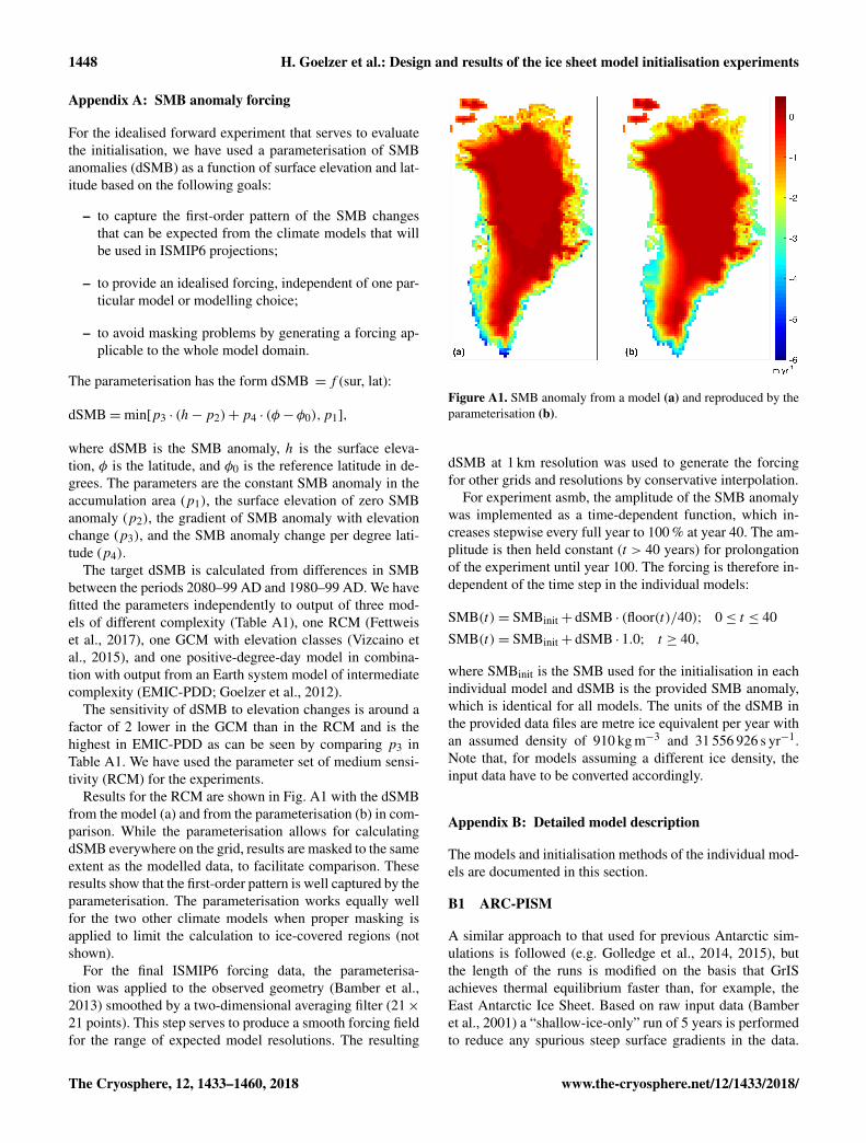
Appendix A: SMB anomaly forcing
For the idealised forward experiment that serves to evaluatethe initialisation, we have used a parameterisation of SMBanomalies (dSMB) as a function of surface elevation and lat-itude based on the following goals:
– to capture the first-order pattern of the SMB changesthat can be expected from the climate models that willbe used in ISMIP6 projections;
– to provide an idealised forcing, independent of one par-ticular model or modelling choice;
– to avoid masking problems by generating a forcing ap-plicable to the whole model domain.
The parameterisation has the form dSMB = f (sur, lat):
dSMB=min[p3 · (h−p2)+p4 · (φ−φ0),p1],
where dSMB is the SMB anomaly, h is the surface eleva-tion, φ is the latitude, and φ0 is the reference latitude in de-grees. The parameters are the constant SMB anomaly in theaccumulation area (p1), the surface elevation of zero SMBanomaly (p2), the gradient of SMB anomaly with elevationchange (p3), and the SMB anomaly change per degree lati-tude (p4).
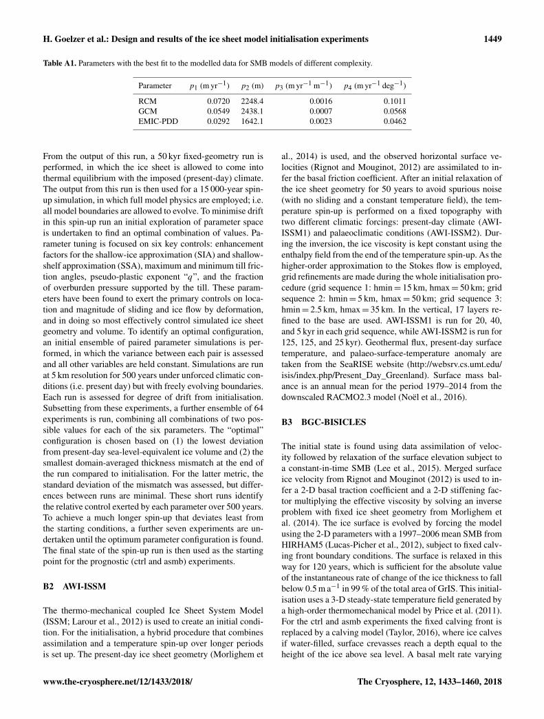
The target dSMB is calculated from differences in SMBbetween the periods 2080–99 AD and 1980–99 AD. We havefitted the parameters independently to output of three mod-els of different complexity (Table A1), one RCM (Fettweiset al., 2017), one GCM with elevation classes (Vizcaino etal., 2015), and one positive-degree-day model in combina-tion with output from an Earth system model of intermediatecomplexity (EMIC-PDD; Goelzer et al., 2012).
The sensitivity of dSMB to elevation changes is around afactor of 2 lower in the GCM than in the RCM and is thehighest in EMIC-PDD as can be seen by comparing p3 inTable A1. We have used the parameter set of medium sensi-tivity (RCM) for the experiments.
Results for the RCM are shown in Fig. A1 with the dSMBfrom the model (a) and from the parameterisation (b) in com-parison. While the parameterisation allows for calculatingdSMB everywhere on the grid, results are masked to the sameextent as the modelled data, to facilitate comparison. Theseresults show that the first-order pattern is well captured by theparameterisation. The parameterisation works equally wellfor the two other climate models when proper masking isapplied to limit the calculation to ice-covered regions (notshown).
For the final ISMIP6 forcing data, the parameterisa-tion was applied to the observed geometry (Bamber et al.,2013) smoothed by a two-dimensional averaging filter (21×21 points). This step serves to produce a smooth forcing fieldfor the range of expected model resolutions. The resulting
Figure A1. SMB anomaly from a model (a) and reproduced by theparameterisation (b).
dSMB at 1 km resolution was used to generate the forcingfor other grids and resolutions by conservative interpolation.
For experiment asmb, the amplitude of the SMB anomalywas implemented as a time-dependent function, which in-creases stepwise every full year to 100 % at year 40. The am-plitude is then held constant (t > 40 years) for prolongationof the experiment until year 100. The forcing is therefore in-dependent of the time step in the individual models:
SMB(t)= SMBinit+ dSMB · (floor(t)/40); 0≤ t ≤ 40SMB(t)= SMBinit+ dSMB · 1.0; t ≥ 40,
where SMBinit is the SMB used for the initialisation in eachindividual model and dSMB is the provided SMB anomaly,which is identical for all models. The units of the dSMB inthe provided data files are metre ice equivalent per year withan assumed density of 910 kg m−3 and 31 556 926 s yr−1.Note that, for models assuming a different ice density, theinput data have to be converted accordingly.
Appendix B: Detailed model description
The models and initialisation methods of the individual mod-els are documented in this section.
B1 ARC-PISM
A similar approach to that used for previous Antarctic sim-ulations is followed (e.g. Golledge et al., 2014, 2015), butthe length of the runs is modified on the basis that GrISachieves thermal equilibrium faster than, for example, theEast Antarctic Ice Sheet. Based on raw input data (Bamberet al., 2001) a “shallow-ice-only” run of 5 years is performedto reduce any spurious steep surface gradients in the data.
The Cryosphere, 12, 1433–1460, 2018 www.the-cryosphere.net/12/1433/2018/
H. Goelzer et al.: Design and results of the ice sheet model initialisation experiments 1449
Table A1. Parameters with the best fit to the modelled data for SMB models of different complexity.
Parameter p1 (m yr−1) p2 (m) p3 (m yr−1 m−1) p4 (m yr−1 deg−1)
RCM 0.0720 2248.4 0.0016 0.1011GCM 0.0549 2438.1 0.0007 0.0568EMIC-PDD 0.0292 1642.1 0.0023 0.0462
From the output of this run, a 50 kyr fixed-geometry run isperformed, in which the ice sheet is allowed to come intothermal equilibrium with the imposed (present-day) climate.The output from this run is then used for a 15 000-year spin-up simulation, in which full model physics are employed; i.e.all model boundaries are allowed to evolve. To minimise driftin this spin-up run an initial exploration of parameter spaceis undertaken to find an optimal combination of values. Pa-rameter tuning is focused on six key controls: enhancementfactors for the shallow-ice approximation (SIA) and shallow-shelf approximation (SSA), maximum and minimum till fric-tion angles, pseudo-plastic exponent “q”, and the fractionof overburden pressure supported by the till. These param-eters have been found to exert the primary controls on loca-tion and magnitude of sliding and ice flow by deformation,and in doing so most effectively control simulated ice sheetgeometry and volume. To identify an optimal configuration,an initial ensemble of paired parameter simulations is per-formed, in which the variance between each pair is assessedand all other variables are held constant. Simulations are runat 5 km resolution for 500 years under unforced climatic con-ditions (i.e. present day) but with freely evolving boundaries.Each run is assessed for degree of drift from initialisation.Subsetting from these experiments, a further ensemble of 64experiments is run, combining all combinations of two pos-sible values for each of the six parameters. The “optimal”configuration is chosen based on (1) the lowest deviationfrom present-day sea-level-equivalent ice volume and (2) thesmallest domain-averaged thickness mismatch at the end ofthe run compared to initialisation. For the latter metric, thestandard deviation of the mismatch was assessed, but differ-ences between runs are minimal. These short runs identifythe relative control exerted by each parameter over 500 years.To achieve a much longer spin-up that deviates least fromthe starting conditions, a further seven experiments are un-dertaken until the optimum parameter configuration is found.The final state of the spin-up run is then used as the startingpoint for the prognostic (ctrl and asmb) experiments.
B2 AWI-ISSM
The thermo-mechanical coupled Ice Sheet System Model(ISSM; Larour et al., 2012) is used to create an initial condi-tion. For the initialisation, a hybrid procedure that combinesassimilation and a temperature spin-up over longer periodsis set up. The present-day ice sheet geometry (Morlighem et
al., 2014) is used, and the observed horizontal surface ve-locities (Rignot and Mouginot, 2012) are assimilated to in-fer the basal friction coefficient. After an initial relaxation ofthe ice sheet geometry for 50 years to avoid spurious noise(with no sliding and a constant temperature field), the tem-perature spin-up is performed on a fixed topography withtwo different climatic forcings: present-day climate (AWI-ISSM1) and palaeoclimatic conditions (AWI-ISSM2). Dur-ing the inversion, the ice viscosity is kept constant using theenthalpy field from the end of the temperature spin-up. As thehigher-order approximation to the Stokes flow is employed,grid refinements are made during the whole initialisation pro-cedure (grid sequence 1: hmin= 15 km, hmax= 50 km; gridsequence 2: hmin= 5 km, hmax= 50 km; grid sequence 3:hmin= 2.5 km, hmax= 35 km. In the vertical, 17 layers re-fined to the base are used. AWI-ISSM1 is run for 20, 40,and 5 kyr in each grid sequence, while AWI-ISSM2 is run for125, 125, and 25 kyr). Geothermal flux, present-day surfacetemperature, and palaeo-surface-temperature anomaly aretaken from the SeaRISE website (http://websrv.cs.umt.edu/isis/index.php/Present_Day_Greenland). Surface mass bal-ance is an annual mean for the period 1979–2014 from thedownscaled RACMO2.3 model (Noël et al., 2016).
B3 BGC-BISICLES
The initial state is found using data assimilation of veloc-ity followed by relaxation of the surface elevation subject toa constant-in-time SMB (Lee et al., 2015). Merged surfaceice velocity from Rignot and Mouginot (2012) is used to in-fer a 2-D basal traction coefficient and a 2-D stiffening fac-tor multiplying the effective viscosity by solving an inverseproblem with fixed ice sheet geometry from Morlighem etal. (2014). The ice surface is evolved by forcing the modelusing the 2-D parameters with a 1997–2006 mean SMB fromHIRHAM5 (Lucas-Picher et al., 2012), subject to fixed calv-ing front boundary conditions. The surface is relaxed in thisway for 120 years, which is sufficient for the absolute valueof the instantaneous rate of change of the ice thickness to fallbelow 0.5 m a−1 in 99 % of the total area of GrIS. This initial-isation uses a 3-D steady-state temperature field generated bya high-order thermomechanical model by Price et al. (2011).For the ctrl and asmb experiments the fixed calving front isreplaced by a calving model (Taylor, 2016), where ice calvesif water-filled, surface crevasses reach a depth equal to theheight of the ice above sea level. A basal melt rate varying
www.the-cryosphere.net/12/1433/2018/ The Cryosphere, 12, 1433–1460, 2018
1450 H. Goelzer et al.: Design and results of the ice sheet model initialisation experiments
between 0 and 4 times the ice thickness is also applied inregions where ice is close to fracture.
B4 DMI-PISM
A spin-up over one full glacial cycle (125 kyr BP to present)is performed with the following guidelines: a freely evolvingrun that inherits the climate memory of the last glacial–interglacial cycle and shall represent the currently observedice sheet state for the contemporary ”year of assignment”.Since we at DMI focus on coupled climate model–ice sheetmodel simulations, we value a free run that is consistentwith the applied forcing higher than a perfect representationof the current observed Greenlandic ice sheet state, suchas ice sheet geometry. We have found that this procedureis necessary to avoid strong unnatural drifts in the icesheet model component after the full coupling betweenthe climate model and the ice sheet model is established(Svendsen et al., 2015). The spin-up first goes throughone complete glacial–interglacial cycle using as a basisthe ERA-Interim reanalysis of the period 1979–2012 todetermine the SMB via PDDs. The scaling of the datasets is determined based on the Greenland temperatureindex in the SeaRISE Greenland data set (based on icecore data; source SeaRISE reference data set: Green-land_SeaRISE_dev1.2.nc). Temporal evolution of the sealevel is also taken from the same SeaRISE Greenland dataset. The ensemble of runs (PISM1, PISM2, PISM3, PISM4,PISM5) differs in the forcing applied to the GrIS. In all casesthe forcing source is based on the ERA-Interim reanalysiscovering the period 1979–2012. The only differences are theapplied PDD factors for the determination of the SMB viaPDDs. The following enumeration lists the applied differentPDD factors: PISM0: PDD_snow = 0.012 m C−1 day−2,PDD_ice = 0.018 m C−1 day−2; PISM1: PDD_snow =0.010 m C−1 day−2, PDD_ice = 0.016 m C−1 day−2;PISM2: PDD_snow = 0.009 m C−1 day−2,PDD_ice = 0.014 m C−1 day−2; PISM3: PDD_snow =0.008 m C−1 day−2, PDD_ice = 0.012 m C−1 day−2;PISM4 PDD_snow = 0.004 m C−1 day−2, PDD_ice =0.008 m C−1 day−2.
B5 IGE-ELMER
The model is initialised using an inverse control method asin Gillet-Chaulet et al. (2012). For the momentum equations,we solve the shelfy-stream approximation. The vertically av-eraged viscosity is constant in all simulations and is ini-tialised using the temperature field coming from a palaeo-spin-up (125 kyr) of the SICOPOLIS model. The limit ofthe model domain is fixed and corresponds to the bound-ary with the ocean: calving front positions are fixed, andthe calving rate is computed as the opposite of the ice fluxthrough the boundary; land-terminated parts can freely re-treat or advance up to the domain limit. The ice sheet topog-
raphy is initialised using the IceBridge BedMachine Green-land V2 data set (Morlighem et al., 2014, 2015), where miss-ing values for the bathymetry around Greenland have beenfilled using data from Bamber et al. (2013). We use a linearbasal friction law. The basal friction coefficient is constantin all transient simulations and is initialised with the controlmethod so that the mismatch between observed and modelledvelocities is minimum. As observations, we use a compos-ite from the NASA Making Earth System Data Records forUse in Research Environments (MEaSUREs) Greenland IceSheet Velocity Map (V1) (Joughin et al., 2010a, b). The icesheet model is then relaxed for 20 years using a 1989–2008mean SMB from the regional climate model MAR (Fettweiset al., 2017) forced with ERA-Interim. The only differencebetween IGE-ELMER1 and IGE-ELMER2 is the mesh reso-lution as given in Table 3.
B6 ILTS-SICOPOLIS
The model is SICOPOLIS version 3.3-dev in SIA modeand with the melting-cold-temperature transition surface en-thalpy method for ice thermodynamics by Greve and Blatter(2016). The present-day surface temperature parameterisa-tion is by Fausto et al. (2009), the present-day precipitationis by Ettema et al. (2009), and the geothermal heat flux isby Greve and Herzfeld (2013) (slightly modified version ofthe heat flux map by Greve, 2005). A spin-up over the lastglacial–interglacial period (125 000 years) is carried out. Ex-cept for initial and final 100-year phases with freely evolv-ing surface and bedrock topography, the topography is keptfixed during the spin-up, whereas the temperature evolvesfreely. This is essentially the method that was used for theSeaRISE experiments (documented in detail by Greve andHerzfeld, 2013). The time-dependent forcing for the spin-upis the GRIP δ18O record (Dansgaard et al., 1993; Johnsen etal., 1997) converted to a purely time-dependent surface tem-perature anomaly 1T by the conversion factor 2.4 ◦C ‰−1
(Huybrechts, 2002).
B7 ILTSPIK-SICOPOLIS
The model version, thermodynamics solver, and present-day surface temperature parameterisation are the same aslisted in Sect. B6. The present-day precipitation is by Robin-son et al. (2010), and the geothermal heat flux is producedby Purucker (https://core2.gsfc.nasa.gov/research/purucker/heatflux_updates.html) following the technique described inFox Maule et al. (2005). The bedrock topography is fromHerzfeld et al., (2014). The ice discharge parameterisationby Calov et al. (2015), Eq. (3) therein with the discharge pa-rameter c = 370 m3 s−1, is applied. A spin-up over the lastglacial–interglacial period (135 000 years) with free evolu-tion of all fields (including the ice sheet topography) is car-ried out. The time-dependent forcing for the spin-up is theGRIP δ18O record (Dansgaard et al., 1993; Johnsen et al.,
The Cryosphere, 12, 1433–1460, 2018 www.the-cryosphere.net/12/1433/2018/
H. Goelzer et al.: Design and results of the ice sheet model initialisation experiments 1451
1997) on the GICC05 timescale (Svensson et al., 2008),converted to a purely time-dependent surface temperatureanomaly 1T by the conversion factor 2.4 ◦C ‰−1, and fur-ther a 7.3 % gain of the precipitation rate for every 1 ◦C in-crease of 1T (Huybrechts, 2002).
B8 IMAU-IMAUICE
The model (de Boer et al., 2014) is initialised to a thermo-dynamically coupled steady state with constant present-dayboundary conditions for 200 kyr using the average 1960–1990 surface temperature and SMB from RACMO2.3 (vanAngelen et al., 2014), extended to outside of the observedice sheet mask using the SMB gradient method (Helsen etal., 2012). Bedrock data are from Bamber et al. (2013),and geothermal heat flux data are from Shapiro and Ritz-woller (2004). The model is run in SIA mode with ice sheetmargins evolving freely within the observed coast mask, out-side of which ice thickness is set to zero.
B9 JPL-ISSM
The ice sheet configuration is set up using data assimilationof present-day conditions and historical spin-up similar to thestudy of Schlegel et al. (2013). SSA is used over the entiredomain with a resolution varying between 1 km in the fast-flowing areas and along the coast and 15 km in the interior.Grounding line migration is based on hydrostatic equilibriumand a sub-element scheme (Seroussi et al., 2014). Observedsurface velocities (Rignot and Mouginot, 2012) are first usedto infer unknown basal friction at the base of the ice sheet(Morlighem et al., 2010). Ice temperature is modelled as-suming the ice sheet to be in a steady-state thermal equi-librium (Seroussi et al., 2013). A spin-up of 50 000 years isthen done to relax the ice sheet model (Larour et al., 2012)and reduce the initial unphysical transient behaviour due toerrors and biases in the data sets (Schlegel et al., 2016) usingmean surface mass balance from 1979 to 1988 (Box, 2013).A historical spin-up is then done from 1840 to 2012 usingreconstructions of surface mass balance for this period (Box,2013). Bedrock topography is interpolated from the BedMa-chine data set (Morlighem et al., 2014), which combines amass conservation algorithm for the fast-flowing ice streamsand kriging in the interior of the ice sheet. Initial ice thicknessis from the Greenland Ice Mapping Project (GIMP) data set(Howat et al., 2014). Geothermal flux is from Shapiro andRitzwoller (2004); air temperature is from RACMO2 (vanAngelen et al., 2014). SMB from a mass balance reconstruc-tion (Box, 2013) averaged over the 2000–2012 period is usedin the ctrl experiment.
B10 LANL-CISM
The ice sheet was initialised with present-day geometryand an idealised temperature profile, and then spun up for20 000 years using pre-1990 climatological surface mass bal-
ance and surface air temperature from RACMO2. No glacialdata were used. The model was spun up for 20 000 years toequilibrate the temperature and geometry with the forcing.The model was initialised (prior to spin-up) with present-daytopography and thickness based on the mass-conserving bedmethod of Morlighem et al. (2011). The SMB over the icesheet was a 1961–1990 climatology from RACMO2. In gridcells where RACMO2 did not provide an SMB, the SMB wasset arbitrarily to −2 m yr−1. Surface air temperatures werealso from a 20th-century RACMO2 climatology (Ettema etal., 2009). The geothermal flux was set spatially uniform to0.05 W m−2.
B11 LSCE-GRISLI
The GRISLI spin-up procedure is based on an iterative dataassimilation method to infer the basal drag from the observedsurface velocities. The first step consists of a 30 kyr equilib-rium simulation of the internal temperature with prescribedice sheet topography (Bamber et al., 2013), 1979–2005 av-eraged near-surface air temperature (Fettweis et al., 2017),geothermal heat flux (Fox Maule et al., 2005), surface veloc-ities (Joughin at al., 2013), and spatially variating basal dragcoefficient from a previous GRISLI experiment (Edwards etal., 2014b). From the resulting internal fields, the 1979–2005mean SMB and near-surface air temperature (Fettweis et al.,2017) are used to run a succession of eight 220 yr simula-tions. During the first 20 years, the basal drag coefficientis corrected to limit the deviation from prescribed veloci-ties, and then the basal drag is kept constant for 200 yearsof surface relaxation. At each iteration, we update the basaldrag coefficient with the value computed at the previous it-eration. The prescribed velocities are the observed velocitiescorrected for thickness differences at the end of the 220 yearsin order to keep the ice flux in GRISLI identical to the ob-served one. Then, a second temperature equilibrium is run forconsistency between the temperature field and the inferredbasal drag coefficient. From this, an additional 220 yr simu-lation is run to optimise the final basal drag coefficient. Thisbasal drag coefficient and associated final ice sheet condi-tions are used as initial conditions for all the initMIP GRISLIexperiments.
B12 MIROC-ICIES1
The simulation set-up of MIROC-IcIES1 is described in Ap-pendix A of Saito et al. (2016), as the experiment E′′s:e1:vm.The surface mass balance field to force the ice sheet modelfollows the present-day field provided by SeaRISE, with-out any correction except for the horizontal resolution. Thismass balance is computed using a PDD method, and the pa-rameters are described at http://websrv.cs.umt.edu/isis/index.php/Future_Climate_Data. The field of basal sliding coeffi-cients are relaxed such that the simulated ice sheet topogra-phy under the present-day surface mass balance field mostly
www.the-cryosphere.net/12/1433/2018/ The Cryosphere, 12, 1433–1460, 2018
1452 H. Goelzer et al.: Design and results of the ice sheet model initialisation experiments
matches the observed geometry, using the method by Pollardand DeConto (2012b). Using the deduced basal sliding co-efficients field, a steady-state spin-up under present-day cli-mate conditions with the fixed geometry is performed againwhile the temperature evolves freely.
B13 MIROC-ICIES2
The simulation set-up of MIROC-IcIES2 is described inSaito et al. (2016), as the experiment B′:v2. A free spin-upover 125 000 years is performed following the SeaRISE con-figuration: the background temperature history based on theoxygen isotope record of the GRIP ice core is used as ananomaly to the present-day field. During the spin-up, the icesheet margin is allowed to freely advance and retreat. Thepresent-day surface temperature follows the parameterisa-tion presented in Fausto et al. (2009). The present-day meanannual precipitation follows Ettema et al. (2009). The sur-face mass balance is computed using these fields and a PDDmethod whose coefficients follow those in Huybrechts and deWolde (1999). The basal sliding velocity is computed usingthe Weertman sliding law, with an allowance for sub-meltsliding following Hindmarsh and Le Meur (2001). The pa-rameters are kept constant and follow those in Huybrechtsand de Wolde (1999) except that the coefficient is doubled toobtain a better match with the present-day topography.
B14 MPIM-PISM
A spin-up over one full glacial cycle (135 kyr BP to present)is performed, where model parameters are changed at 20 kyrBP. It is faster to start from a pre-spun up state at 20 kyrBP than to re-run the full glacial cycle for each parameterchange. The spin-up first goes through one complete glacialcycle using a linear combination of MPI-ESM output. Thescaling of the two data sets is determined based on the Green-land temperature index in the SeaRISE Greenland data set(based on GRIP data). Sea-level changes are also taken fromthe SeaRISE Greenland data set.
B15 UAF-PISM
A spin-up over a glacial cycle is combined with a short re-laxation run. To define the energy state, a “standard” glacialcycle run is performed where the surface can evolve freely,similar to Aschwanden et al. (2013) and Aschwanden etal. (2016). The spin-up starts at 125 kyr BP with the present-day topography from Howat et al. (2014) using a horizon-tal grid resolution of 9 km. The grid is refined to 6, 4.5, and3 km at 25, 20, and 15 kyr BP, respectively. We use a positive-degree-day scheme to compute the climatic mass balancefrom surface temperature (Fausto et al., 2009) and model-constrained precipitation (Ettema et al., 2009). The degree-day factors are the same as in Huybrechts (1999). Second,we account for palaeoclimatic variations by applying a scalaranomaly term derived from the GRIP ice core oxygen iso-
tope record (Dansgaard et al., 1993) to the temperature field(Huybrechts, 2002). Then we adjust mean annual precipita-tion in proportion to the mean annual air temperature change(Huybrechts, 2002). Finally, sea-level forcing, which deter-mines the land area available for glaciation, is derived fromthe SPECMAP marine δ18O record (Imbrie et al., 1992). Atthe end of the spin-up, the computed surface elevation differsfrom the observed surface elevation. From here we performtwo sets of 60-year relaxation simulations using the RACMO1960–1990 averaged climatic mass balance. In one set (UAF-PISM4–6), we regrid the spun-up state from the 3 km sim-ulation to 1.5 km (UAF-PISM4), 3 km (UAF-PISM5) and4.5 km (UAF-PISM6) and run a relaxation where the icesheet is free to evolve. At the end of this relatively shortrelaxation, the computed surface elevation continues to dif-fer substantially from present-day observation, and the modelstates exhibit a large artificial drift. To reduce the mismatchbetween observed and simulated surface elevations, we per-form a second set, UAF-PISM1–3. Here we regrid the energystate in the ice and in the bedrock from the spun-up state fromthe 3 km simulation to 1.5 km (UAF-PISM1), 3 km (UAF-PISM2), and 4.5 km (UAF-PISM3) and combine those fieldswith the present-day topography from Howat et al. (2014) toagain run a relaxation where the ice sheet is free to evolve.
B16 UCIJPL-ISSM
The ice sheet configuration is set up using data assimila-tion of present-day conditions (Morlighem et al., 2010). Arelaxation of 50 years is then performed to reduce the ini-tial unphysical transient behaviour due to errors and biasesin the data sets (Seroussi et al., 2011), using mean surfacemass balance from 1961 to 1990 (van Angelen et al., 2014).A higher-order model (HO) is used for the entire domain,with 14 vertical layers and a horizontal resolution varyingbetween 0.5 km along the coast and 30 km inland. We per-form the inversion of basal friction assuming that the ice isin thermomechanical steady state. The ice temperature is up-dated as the basal friction changes, and the ice viscosity ischanged accordingly. At the end of the inversion, basal fric-tion, ice temperature, and stresses are all consistent. Afterthe data assimilation, the model is relaxed for 50 years usingthe mean surface mass balance of 1961–1990 from RACMO(van Angelen et al., 2014), while keeping the temperatureconstant. Bed topography is interpolated from the BedMa-chine Greenland v3 data set (Morlighem et al., 2017), whichcombines a mass conservation algorithm for the fast-flowingice streams and kriging in the interior of the ice sheet. Initialice surface topography is from the GIMP data set (Howat etal., 2014). For the thermal model, surface temperatures fromFausto et al. (2009) and geothermal heat flux from Shapiroand Ritzwoller (2004) are used. Mean surface mass balanceof 1961–1990 from RACMO (van Angelen et al., 2014) isused in the ctrl experiment.
The Cryosphere, 12, 1433–1460, 2018 www.the-cryosphere.net/12/1433/2018/
H. Goelzer et al.: Design and results of the ice sheet model initialisation experiments 1453
B17 ULB-FETISH
Model initialisation is based on the method by Pollard andDeConto (2012b) by optimising basal sliding coefficientsfor the grounded ice sheet in an iterative way through min-imising the misfit between observed and modelled surfacetopography. A regularisation term is introduced to smoothhigh-frequency noise in the basal sliding coefficients (Pat-tyn, 2017). Initial ice sheet surface and bedrock elevation aretaken from Bamber et al. (2013), and geothermal heat fluxstems from Fox Maule et al. (2009). The initialisation runsover a period of 50 000 years forced by a constant surfacemass balance (Fettweis et al., 2007) and surface temperature(Fausto et al., 2009). During this time, the marine boundariesare kept fixed in space. For the control and forcing runs, thegrounded ice margin and grounding line are allowed to movefreely, starting from the initialised state. Two model setupswere considered: FETISH1 is according to SIA; FETISH2is a hybrid model (superimposed SSA-SIA) with a flux con-dition at the grounding line according to Schoof (2007) andPollard and DeConto (2012a).
B18 VUB-GISM
The model is initialised with a glacial spin-up over the lasttwo glacial cycles and recent climate forcing data up to theyear 2005 (Fürst et al., 2015). For the spin-up, a synthe-sised temperature record is used based on ice core data fromDome C, NGRIP, GRIP, and GISP2 (Barker et al., 2011; An-dersen et al., 2004; Dansgaard et al., 1993; Kobashi et al.,2011), and precipitation is scaled by 5 % per degree Cel-sius. For the period 1958 to 2005, the atmospheric forcingcomes from a combination of European Centre for Medium-Range Weather Forecasts (ECMWF) ERA-Interim meteo-rological reanalysis and ECMWF operational analysis data.Use is made of monthly temperature anomalies and yearlyprecipitation ratios. The ocean forcing from 1958 to 2005 de-rives from a CMIP5 model providing temperature anomaliesat mid-depth (300–800 m) in five surrounding ocean basinswith respect to the 1960–1990 period. After the year 2005,atmospheric and oceanic forcings are reset to their 1960–1990 averages in the unforced state. Bedrock elevation andcoast mask are based on Bamber et al. (2013); the pattern ofsurface accumulation for the period 1950–2000 is based onBales et al. (2009). The higher-order model (GISM1) is ini-tialised with an SIA model (GISM2) to 3 kyr BP. Switchingat 3 kyr BP appeared to be sufficiently early to resolve themain effects of including horizontal stress gradients by thepresent day.
Appendix C: Data request
The requested variables (Table C1) serve to evaluate andcompare the different models and initialisation techniques.
All 2-D data were requested on a regular grid withthe following description: polar stereographic projectionwith standard parallel at 71◦ N and a central meridian of39◦W (321◦ E) on datum WGS84. The lower left corneris at (−800 000 m, −3 400 000 m), and the upper right at(700 000 m, −600 000 m). This is the same grid (Bamber etal., 2001) as used to provide the SMB anomaly forcing. Theoutput was submitted on a resolution adapted to the resolu-tion of the model and was 5 or 10 km. The data were conser-vatively interpolated to 5 km resolution for diagnostic pro-cessing.
If interpolation was required in order to transform theSMB forcing (1 km, same as Bamber et al., 2013) to the na-tive model grid, and transform model output to the initMIPoutput grid (20, 10, 5, 1 km; Bamber et al., 2001), it was re-quested that conservative interpolation be used. The motiva-tion for using a common method for all models is to minimisemodel-to-model differences due to the choice of interpola-tion methods. In most cases this has been followed by themodellers.
We distinguish between state variables (e.g. ice thickness,temperatures, and velocities) and flux variables (e.g. SMB).State variables were requested as snapshot information atthe end of 1-year (scalars) and 5-year periods (2-D), whileflux variables were averaged over the respective periods. Forcalculation of scalar diagnostics (e.g. total ice mass or ice-covered area), it is necessary to correct for the area dis-tortions implicit for a given projection (e.g. Snyder, 1987).Some of the variables may not be applicable for each model,in which case they were omitted.
Please note that, in order to facilitate comparison with ob-servational data sets and for consistency with future ISMIP6activities, all model output data from initMIP-Greenlandpublished to public archives have been conservatively inter-polated to a new diagnostic grid. The grid uses EPSG:3413, apolar stereographic projection with standard parallel at 70◦ Nand a central meridian of 45◦W on datum WGS84.
www.the-cryosphere.net/12/1433/2018/ The Cryosphere, 12, 1433–1460, 2018

1454 H. Goelzer et al.: Design and results of the ice sheet model initialisation experiments
Table C1. Data request for participation in initMIP-Greenland. Type: FL – flux variable; ST – state variable; CST – constant.
Variable name Units Type Standard name (CF)
Ice sheet altitude m ST surface_altitudeIce sheet thickness m ST land_ice_thicknessBedrock altitude m ST bedrock_altitudeBedrock geothermal heat flux W m−2 CST upward_geothermal_heat_flux_at_ground_level_in_land_iceSurface mass balance flux kg m−2 s−1 FL land_ice_surface_specific_mass_balance_fluxBasal mass balance flux kg m−2 s−1 FL land_ice_basal_specific_mass_balance_fluxLand ice calving flux kg m−2 s−1 FL land_ice_specific_mass_flux_due_to_calvingIce thickness imbalance m s−1 FL tendency_of_land_ice_thicknessX component of land ice surface velocity m s−1 ST land_ice_surface_x_velocityY component of land ice surface velocity m s−1 ST land_ice_surface_y_velocityZ component of land ice surface velocity m s−1 ST land_ice_surface_upward_velocityX component of land ice basal velocity m s−1 ST land_ice_basal_x_velocityY component of land ice basal velocity m s−1 ST land_ice_basal_y_velocityZ component of land ice basal velocity m s−1 ST land_ice_basal_upward_velocityX component of land ice vertical mean velocity m s−1 ST land_ice_vertical_mean_x_velocityY component of land ice vertical mean velocity m s−1 ST land_ice_vertical_mean_y_velocitySurface temperature of ice sheet K ST temperature_at_top_of_ice_sheet_modelBasal temperature of ice sheet K ST temperature_at_base_of_ice_sheet_modelBasal drag Pa ST land_ice_basal_dragLand ice area fraction 1 ST land_ice_area_fractionGrounded ice area fraction 1 ST grounded_ice_sheet_area_fractionFloating ice shelf area fraction 1 ST floating_ice_shelf_area_fractionIce mass kg ST land_ice_massIce mass not displacing seawater kg ST land_ice_mass_not_displacing_sea_waterArea covered by grounded ice m2 ST grounded_ice_sheet_areaArea covered by floating ice m2 ST floating_ice_shelf_areaTotal SMB flux kg s−1 FL tendency_of_land_ice_mass_due_to_surface_mass_balanceTotal BMB flux kg s−1 FL tendency_of_land_ice_mass_due_to_basal_mass_balanceTotal calving flux kg s−1 FL tendency_of_land_ice_mass_due_to_calving
The Cryosphere, 12, 1433–1460, 2018 www.the-cryosphere.net/12/1433/2018/
H. Goelzer et al.: Design and results of the ice sheet model initialisation experiments 1455
The Supplement related to this article is available onlineat https://doi.org/10.5194/tc-12-1433-2018-supplement.
Competing interests. The authors declare that they have no conflictof interest.
Acknowledgements. We acknowledge the Climate and Cryosphere(CliC) project and the World Climate Research Programme(WCRP) for their guidance, support, and sponsorship. We thankthe CMIP6 panel members for their continuous leadership of theCMIP6 effort, and the Working Group on Coupled Modeling(WGCM) Infrastructure Panel (WIP) for overseeing the CMIP6 andISMIP6 infrastructure and data request. We would like to thankBrice Noël for help with the SMB validation data and Xavier Fet-tweis, Miren Vizcaino, and Vincent Cabot for providing SMB data.We also thank Erika Simon for help with the data processing.
Andy Aschwanden, Eric Larour, Sophie Nowicki, and HeleneSeroussi were supported by grants from the NASA CryosphericScience Program and Modeling, Analysis, and Prediction Program.Heiko Goelzer has received funding from the programme of theNetherlands Earth System Science Centre (NESSC), financiallysupported by the Dutch Ministry of Education, Culture and Science(OCW) under grant no. 024.002.001. Nicholas R. Golledge issupported by Royal Society of New Zealand Rutherford DiscoveryFellowship 15-VUW-004. Philippe Huybrechts acknowledgessupport from the iceMOD project funded by the Research Foun-dation – Flanders (FWO-Vlaanderen). William H. Lipscomb andJoseph H. Kennedy were supported by the Regional and GlobalClimate Modeling and Earth System Modeling programmesof the U.S. Department of Energy’s Office of Science. TheNational Center for Atmospheric Research is sponsored by theNational Science Foundation. Victoria Lee, Stephen L. Cornford,and Antony J. Payne carried out work as part of the UKESMcontribution for CMIP6. Mathieu Morlighem was supported byNASA’s Cryospheric Sciences Program (no. NNX15AD55G)and the National Science Foundation’s Arctic System ScienceProgram (ARCSS) (no. 1504230). Christian Rodehacke (DMI)has received funding from the European Research Council underthe European Community’s Seventh Framework Programme(FP7/2007–2013)/ERC grant agreement 610055 as part of theIce2Ice project as well as the Nordic Center of Excellence eSTICC(eScience Tool for In-vestigating Climate Change in northern highlatitudes) funded by Nordforsk (grant 57001). Florian A. Ziemenwas supported by the BMBF project PALMOD. Computationalresources for MPI-PISM were made available by DKRZ throughsupport from BMBF. IGE-ELMER simulations were performedusing the Froggy platform of the CIMENT infrastructure – whichis supported by the Rhône-Alpes region (grant CPER07_13 CIRA),the OSUG@2020 laBex (reference ANR10 LABX56), and theEquip@Meso project (reference ANR-10-EQPX-29-01) – andusing HPC resources from GENCI-CINES (grant 2016-016066).Ralf Greve, Ayako Abe-Ouchi, and Fuyuki Saito were supportedby the Arctic Challenge for Sustainability (ArCS) project of theJapanese Ministry of Education, Culture, Sports, Science andTechnology (MEXT), and by the Japan Society for the Promotionof Science (JSPS) KAKENHI under grant no. 17H06104, Ralf
Greve and Ayako Abe-Ouchi were additionally supported underJSPS grant no. 16H02224, and Fuyuki Saito under JSPS grant no.17K05664. Ayako Abe-Ouchi and Fuyuki Saito were supported bythe Integrated Research Program for Advancing Climate Models(TOUGOU program) from MEXT. Reinhard Calov was funded bythe Leibniz Association grant SAW-2014-PIK-1 and is now fundedby the Bundesministerium für Bildung und Forschung (BMBF)grants PalMod-1.1-TP5 and PalMod-1.3-TP4.
Edited by: G. Hilmar GudmundssonReviewed by: two anonymous referees
References
Adalgeirsdottir, G., Aschwanden, A., Khroulev, C., Boberg,F., Mottram, R., Lucas-Picher, P., and Christensen, J. H.:Role of model initialization for projections of 21st-centuryGreenland ice sheet mass loss, J. Glaciol., 60, 782–794,https://doi.org/10.3189/2014JoG13J202, 2014.
Alexander, P. M., Tedesco, M., Schlegel, N.-J., Luthcke, S.B., Fettweis, X., and Larour, E.: Greenland Ice Sheet sea-sonal and spatial mass variability from model simulationsand GRACE (2003–2012), The Cryosphere, 10, 1259–1277,https://doi.org/10.5194/tc-10-1259-2016, 2016.
Andersen, K., Azuma, N., Barnola, J., Bigler, M., Biscaye, P., Cail-lon, N., Chappellaz, J., Clausen, H., DahlJensen, D., Fischer, H.,Fluckiger, J., Fritzsche, D., Fujii, Y., Goto-Azuma, K., Gron-vold, K., Gundestrup, N., Hansson, M., Huber, C., Hvidberg, C.,Johnsen, S., Jonsell, U., Jouzel, J., Kipfstuhl, S., Landais, A.,Leuenberger, M., Lorrain, R., Masson-Delmotte, V., Miller, H.,Motoyama, H., Narita, H., Popp, T., Rasmussen, S., Raynaud, D.,Rothlisberger, R., Ruth, U., Samyn, D., Schwander, J., Shoji, H.,Siggard-Andersen, M., Steffensen, J., Stocker, T., Sveinbjorns-dottir, A., Svensson, A., Takata, M., Tison, J., Thorsteinsson,T., Watanabe, O., Wilhelms, F., White, J., and Project, N. G. I.C.: High-resolution record of Northern Hemisphere climate ex-tending into the last interglacial period, Nature, 431, 147–151,https://doi.org/10.1038/nature02805, 2004.
Arthern, R. and Gudmundsson, G.: Initialization of ice-sheet fore-casts viewed as an inverse Robin problem, J. Glaciol., 56, 527–533, 2010.
Arthern, R. J., Hindmarsh, R. C. A., and Williams, C. R.:Flow speed within the Antarctic ice sheet and its controls in-ferred from satellite observations, J. Geophys. Res.-Earth, 120,2014JF003239, https://doi.org/10.1002/2014JF003239, 2015.
Asay-Davis, X. S., Cornford, S. L., Durand, G., Galton-Fenzi, B.K., Gladstone, R. M., Gudmundsson, G. H., Hattermann, T., Hol-land, D. M., Holland, D., Holland, P. R., Martin, D. F., Mathiot,P., Pattyn, F., and Seroussi, H.: Experimental design for threeinterrelated marine ice sheet and ocean model intercomparisonprojects: MISMIP v. 3 (MISMIP+), ISOMIP v. 2 (ISOMIP +)and MISOMIP v. 1 (MISOMIP1), Geosci. Model Dev., 9, 2471–2497, https://doi.org/10.5194/gmd-9-2471-2016, 2016.
Aschwanden, A., Aðalgeirsdóttir, G., and Khroulev, C.: Hindcast-ing to measure ice sheet model sensitivity to initial states, TheCryosphere, 7, 1083–1093, https://doi.org/10.5194/tc-7-1083-2013, 2013.
www.the-cryosphere.net/12/1433/2018/ The Cryosphere, 12, 1433–1460, 2018
1456 H. Goelzer et al.: Design and results of the ice sheet model initialisation experiments
Aschwanden, A., Fahnestock, M. A., and Truffer, M.: ComplexGreenland outlet glacier flow captured, Nat. Commun., 7, 10524,https://doi.org/10.1038/ncomms10524, 2016.
Bales, R. C., Guo, Q., Shen, D., Mcconnell, J. R., Du, G.,Burkhart, J. F., Spikes, V. B., Hanna, E., and Cappelen,J.: Annual accumulation for Greenland updated using icecore data developed during 2000–2006 and analysis of dailycoastal meteorological data, J. Geophys. Res., 114, D06116,https://doi.org/10.1029/2008JD011208, 2009.
Bamber, J. L., Ekholm, S., and Krabill, W. B.: A new, high-resolution digital elevation model of Greenland fully validatedwith airborne laser altimeter data, J. Geophys. Res., 106, 6733–6745, 2001.
Bamber, J. L., Griggs, J. A., Hurkmans, R. T. W. L., Dowdeswell,J. A., Gogineni, S. P., Howat, I., Mouginot, J., Paden, J.,Palmer, S., Rignot, E., and Steinhage, D.: A new bed el-evation dataset for Greenland, The Cryosphere, 7, 499-510,https://doi.org/10.5194/tc-7-499-2013, 2013.
Barker, S., Knorr, G., Edwards, R. L., Parrenin, F., Putnam,A. E., Skinner, L. C., Wolff, E., and Ziegler, M.: 800,000Years of Abrupt Climate Variability, Science, 334, 347–351,https://doi.org/10.1126/science.1203580, 2011.
Bindschadler, R. A., Nowicki, S., Abe-Ouchi, A., Aschwanden, A.,Choi, H., Fastook, J., Granzow, G., Greve, R., Gutowski, G.,Herzfeld, U., Jackson, C., Johnson, J., Khroulev, C., Levermann,A., Lipscomb, W. H., Martin, M. A., Morlighem, M., Parizek, B.R., Pollard, D., Price, S. F., Ren, D., Saito, F., Sato, T., Seddik,H., Seroussi, H., Takahashi, K., Walker, R., and Wang, W. L.: Ice-sheet model sensitivities to environmental forcing and their usein projecting future sea level (the SeaRISE project), J. Glaciol.,59, 195–224, https://doi.org/10.3189/2013JoG12J125, 2013.
Box, J.: Greenland Ice Sheet Mass Balance Reconstruction. Part II:Surface Mass Balance (1840–2010), J. Climate, 26, 6974–6989,https://doi.org/10.1175/jcli-d-12-00518.1, 2013.
Calov, R., Greve, R., Abe-Ouchi, A., Bueler, E., Huybrechts, P.,Johnson, J., Pattyn, F., Pollard, D., Ritz, C., Saito, F., and Tarasov,L.: Results from the Ice-Sheet Model Intercomparison Project–Heinrich Event INtercOmparison (ISMIP HEINO), J. Glaciol.,56, 371–383, 2010.
Calov, R., Robinson, A., Perrette, M., and Ganopolski, A.: Sim-ulating the Greenland ice sheet under present-day and palaeoconstraints including a new discharge parameterization, TheCryosphere, 9, 179–196, https://doi.org/10.5194/tc-9-179-2015,2015.
Dansgaard, W., Johnsen, S. J., Clausen, H. B., Dahl-Jensen, D.,Gundestrup, N. S., Hammer, C. U., Hvidberg, C. S., Steffensen,J. P., Sveinbjoernsdottir, A. E., Jouzel, J., and Bond, G. C.: Evi-dence for general instability of past climate from a 250-kyr ice-core record, Nature, 364, 218–220, 1993.
de Boer, B., Stocchi, P., and van de Wal, R. S. W.: A fully coupled 3-D ice-sheet–sea-level model: algorithm and applications, Geosci.Model Dev., 7, 2141–2156, https://doi.org/10.5194/gmd-7-2141-2014, 2014.
Drewry, D. J., Morris, E. M., Robin, G. D. Q., and Weller, G.: TheResponse of Large Ice Sheets to Climatic Change, Philos. T. Roy.Soc. B, 338, 235–242, https://doi.org/10.1098/rstb.1992.0143,1992.
Edwards, T. L., Fettweis, X., Gagliardini, O., Gillet-Chaulet, F.,Goelzer, H., Gregory, J. M., Hoffman, M., Huybrechts, P., Payne,
A. J., Perego, M., Price, S., Quiquet, A., and Ritz, C.: Probabilis-tic parameterisation of the surface mass balance–elevation feed-back in regional climate model simulations of the Greenland icesheet, The Cryosphere, 8, 181–194, https://doi.org/10.5194/tc-8-181-2014, 2014a.
Edwards, T. L., Fettweis, X., Gagliardini, O., Gillet-Chaulet, F.,Goelzer, H., Gregory, J. M., Hoffman, M., Huybrechts, P., Payne,A. J., Perego, M., Price, S., Quiquet, A., and Ritz, C.: Effect ofuncertainty in surface mass balance–elevation feedback on pro-jections of the future sea level contribution of the Greenland icesheet, The Cryosphere, 8, 195–208, https://doi.org/10.5194/tc-8-195-2014, 2014b.
Enderlin, E. M., Howat, I. M., Jeong, S., Noh, M.-J., van Angelen, J.H., and van den Broeke, M. R.: An improved mass budget for theGreenland ice sheet, Geophys. Res. Lett., 41, 2013GL059010,https://doi.org/10.1002/2013GL059010, 2014.
Ettema, J., Van Den Broeke, M. R., Van Meijgaard, E., Van De Berg,W. J., Bamber, J. L., Box, J. E., and Bales, R. C.: Higher sur-face mass balance of the Greenland ice sheet revealed by high-resolution climate modeling, Geophys. Res. Lett., 36, L12501,https://doi.org/10.1029/2009GL038110, 2009.
Eyring, V., Bony, S., Meehl, G. A., Senior, C. A., Stevens, B.,Stouffer, R. J., and Taylor, K. E.: Overview of the CoupledModel Intercomparison Project Phase 6 (CMIP6) experimen-tal design and organization, Geosci. Model Dev., 9, 1937–1958,https://doi.org/10.5194/gmd-9-1937-2016, 2016.
Fausto, R. S., Ahlstrøm, A. P., Van As, D., Bøggild, C.E., and Johnsen, S. J.: A new present-day temperatureparameterization for Greenland, J. Glaciol., 55, 95–105,https://doi.org/10.3189/002214309788608985, 2009.
Fettweis, X., Box, J. E., Agosta, C., Amory, C., Kittel, C., Lang, C.,van As, D., Machguth, H., and Gallée, H.: Reconstructions of the1900–2015 Greenland ice sheet surface mass balance using theregional climate MAR model, The Cryosphere, 11, 1015–1033,https://doi.org/10.5194/tc-11-1015-2017, 2017.
Fox Maule, C., Purucker, M. E., Olsen, N., and Mosegaard, K.: Heatflux anomalies in Antarctica revealed by satellite magnetic data,Science, 309, 464–467, 2005.
Franco, B., Fettweis, X., Lang, C., and Erpicum, M.: Impactof spatial resolution on the modelling of the Greenland icesheet surface mass balance between 1990–2010, using theregional climate model MAR, The Cryosphere, 6, 695–711,https://doi.org/10.5194/tc-6-695-2012, 2012.
Fürst, J. J., Goelzer, H., and Huybrechts, P.: Ice-dynamic pro-jections of the Greenland ice sheet in response to atmo-spheric and oceanic warming, The Cryosphere, 9, 1039–1062,https://doi.org/10.5194/tc-9-1039-2015, 2015.
Gillet-Chaulet, F., Gagliardini, O., Seddik, H., Nodet, M., Du-rand, G., Ritz, C., Zwinger, T., Greve, R., and Vaughan, D.G.: Greenland ice sheet contribution to sea-level rise from anew-generation ice-sheet model, The Cryosphere, 6, 1561–1576,https://doi.org/10.5194/tc-6-1561-2012, 2012.
Goelzer, H., Huybrechts, P., Raper, S. C. B., Loutre, M.-F.,Goosse, H., and Fichefet, T.: Millennial total sea-level com-mitments projected with the Earth system model of interme-diate complexity LOVECLIM, Environ. Res. Lett., 7, 1–9,https://doi.org/10.1088/1748-9326/7/4/045401, 2012.
Goelzer, H., Huybrechts, P., Fürst, J. J., Andersen, M. L.,Edwards, T. L., Fettweis, X., Nick, F. M., Payne, A. J.,
The Cryosphere, 12, 1433–1460, 2018 www.the-cryosphere.net/12/1433/2018/
H. Goelzer et al.: Design and results of the ice sheet model initialisation experiments 1457
and Shannon, S. R.: Sensitivity of Greenland ice sheet pro-jections to model formulations, J. Glaciol., 59, 733–749,https://doi.org/10.3189/2013JoG12J182, 2013.
Goelzer, H., Robinson, A., Seroussi, H., and Van De Wal,R. S. W.: Recent Progress in Greenland Ice Sheet Mod-elling, Current Climate Change Reports, 3, 291–302,https://doi.org/10.1007/s40641-017-0073-y, 2017.
Goldberg, D. N. and Heimbach, P.: Parameter and state estima-tion with a time-dependent adjoint marine ice sheet model, TheCryosphere, 7, 1659–1678, https://doi.org/10.5194/tc-7-1659-2013, 2013.
Golledge, N. R., Menviel, L., Carter, L., Fogwill, C. J., England, M.H., Cortese, G., and Levy, R. H.: Antarctic contribution to melt-water pulse 1A from reduced Southern Ocean overturning, Nat.Commun., 5, 5107, https://doi.org/10.1038/ncomms6107, 2014.
Golledge, N. R., Kowalewski, D. E., Naish, T. R., Levy, R. H., Fog-will, C. J., and Gasson, E. G. W.: The multi-millennial Antarc-tic commitment to future sea-level rise, Nature, 526, 421–425,https://doi.org/10.1038/nature15706, 2015.
Greve, R.: Relation of measured basal temperatures andthe spatial distribution of the geothermal heat flux forthe Greenland ice sheet, Ann. Glaciol., 42, 424–432,https://doi.org/10.3189/172756405781812510, 2005.
Greve, R. and Blatter, H.: Comparison of thermodynamics solversin the polythermal ice sheet model SICOPOLIS, Polar Sci., 10,11–23, https://doi.org/10.1016/j.polar.2015.12.004, 2016.
Greve, R. and Herzfeld, U. C.: Resolution of ice streamsand outlet glaciers in large-scale simulations of theGreenland ice sheet, Ann. Glaciol., 54, 209–220,https://doi.org/10.3189/2013AoG63A085, 2013.
Greve, R., Saito, F., and Abe-Ouchi, A.: Initial results of theSeaRISE numerical experiments with the models SICOPOLISand IcIES for the Greenland ice sheet, Ann. Glaciol., 52, 23–30,2011.
Helsen, M. M., van de Wal, R. S. W., van den Broeke, M. R., vande Berg, W. J., and Oerlemans, J.: Coupling of climate modelsand ice sheet models by surface mass balance gradients: appli-cation to the Greenland Ice Sheet, The Cryosphere, 6, 255–272,https://doi.org/10.5194/tc-6-255-2012, 2012.
Herzfeld, U. C., McDonald, B. W., Wallin, B. F., Chen, P.A., Mayer, H., Paden, J., and Leuschen, C. J.: The trough-system algorithm and its application to spatial modeling ofGreenland subglacial topography, Ann. Glaciol., 55, 115–126,https://doi.org/10.3189/2014AoG67A001, 2014.
Hindmarsh, R. C. A. and Le Meur, E.: Dynamical processes in-volved in the retreat of marine ice sheets, J. Glaciol., 47, 271–282, https://doi.org/10.3189/172756501781832269, 2001.
Howat, I. M., Negrete, A., and Smith, B. E.: The Green-land Ice Mapping Project (GIMP) land classification andsurface elevation data sets, The Cryosphere, 8, 1509–1518,https://doi.org/10.5194/tc-8-1509-2014, 2014.
Huybrechts, P.: Sea-level changes at the LGM from ice-dynamicreconstructions of the Greenland and Antarctic ice sheets dur-ing the glacial cycles, Quaternary Sci. Rev., 21, 203–231,https://doi.org/10.1016/S0277-3791(01)00082-8, 2002.
Huybrechts, P. and de Wolde, J.: The dynamic re-sponse of the Greenland and Antarctic ice sheetsto multiple-century climatic warming, J. Cli-
mate, 12, 2169–2188, https://doi.org/10.1175/1520-0442(1999)012<2169:TDROTG>2.0.CO;2, 1999.
Huybrechts, P., Letréguilly, A., and Reeh, N.: The Greenland icesheet and greenhouse warming, Global Planet. Change, 3, 399–412, 1991.
Huybrechts, P., Payne, A. J., and Group, E. I.: The EISMINT bench-marks for testing ice-sheet models, Ann. Glaciol., 23, 1–12,1996.
Huybrechts, P., Janssens, I., Poncin, C., and Fichefet, T.: The re-sponse of the Greenland ice sheet to climate changes in the 21stcentury by interactive coupling of an AOGCM with a thermome-chanical ice-sheet model, Ann. Glaciol., 35, 409–415, 2002.
Imbrie, J., Boyle, E. A., Clemens, S. C., Duffy, A., Howard, W. R.,Kukla, G., Kutzbach, J., Martinson, D. G., McIntyre, A., Mix,A. C., Molfino, B., Morley, J. J., Peterson, L. C., Pisias, N. G.,Prell, W. L., Raymo, M. E., Shackleton, N. J., and Toggweiler,J. R.: On the Structure and Origin of Major Glaciation Cycles 1.Linear Responses to Milankovitch Forcing, Paleoceanography, 7,701–738, https://doi.org/10.1029/92PA02253, 1992.
Johnsen, S. J., Clausen, H. B., Dansgaard, W., Gundestrup, N. S.,Hammer, C. U., Andersen, U., Andersen, K. K., Hvidberg, C. S.,Dahl-Jensen, D., Steffensen, J. P., Shoji, H., Sveinbjörnsdóttir, Á.E., White, J., Jouzel, J., and Fisher, D.: The δ18O record alongthe Greenland Ice Core Project deep ice core and the problem ofpossible Eemian climatic instability, J. Geophys. Res.-Oceans,102, 26397–26410, https://doi.org/10.1029/97JC00167, 1997.
Jones, P. W.: First- and Second-Order Conservative Remap-ping Schemes for Grids in Spherical Coordinates, Mon.Weather Rev., 127, 2204–2210, https://doi.org/10.1175/1520-0493(1999)127<2204:fasocr>2.0.co;2, 1999.
Joughin, I., Smith, B., Howat, I., and Scambos, T.: MEa-SUREs Greenland Ice Sheet Velocity Map from InSARData, Version 1., Boulder, Colorado USA, NASA NationalSnow and Ice Data Center Distributed Active Archive Cen-ter, https://doi.org/10.5067/MEASURES/CRYOSPHERE/nsidc-0478.001, 2010a.
Joughin, I., Smith, B., Howat, I. M., Scambos, T., andMoon, T.: Greenland flow variability from ice-sheet-wide velocity mapping, J. Glaciol., 56, 415–430,https://doi.org/10.3189/002214310792447734, 2010b.
Joughin, I., Smith, B., Howat, I., and Scambos, T.: MEa-SUREs Multi-year Greenland Ice Sheet Velocity Mosaic,Version 1., Boulder, Colorado USA, NASA National Snowand Ice Data Center Distributed Active Archive Center,https://doi.org/10.5067/QUA5Q9SVMSJG, 2016.
Kobashi, T., Kawamura, K., Severinghaus, J. P., Barnola, J.-M.,Nakaegawa, T., Vinther, B. M., Johnsen, S. J., and Box, J. E.:High variability of Greenland surface temperature over the past4000 years estimated from trapped air in an ice core, Geophys.Res. Lett., 38, L21501, https://doi.org/10.1029/2011GL049444,2011.
Larour, E., Seroussi, H., Morlighem, M., and Rignot, E.: Continen-tal scale, high order, high spatial resolution, ice sheet modelingusing the Ice Sheet System Model (ISSM), J. Geophys. Res., 117,F01022, https://doi.org/10.1029/2011JF002140, 2012.
Larour, E., Utke, J., Csatho, B., Schenk, A., Seroussi, H.,Morlighem, M., Rignot, E., Schlegel, N., and Khazendar, A.:Inferred basal friction and surface mass balance of the North-east Greenland Ice Stream using data assimilation of ICESat
www.the-cryosphere.net/12/1433/2018/ The Cryosphere, 12, 1433–1460, 2018
1458 H. Goelzer et al.: Design and results of the ice sheet model initialisation experiments
(Ice Cloud and land Elevation Satellite) surface altimetry andISSM (Ice Sheet System Model), The Cryosphere, 8, 2335–2351,https://doi.org/10.5194/tc-8-2335-2014, 2014.
Larour, E., Utke, J., Bovin, A., Morlighem, M., and Perez, G.:An approach to computing discrete adjoints for MPI-parallelizedmodels applied to Ice Sheet System Model 4.11, Geosci. ModelDev., 9, 3907–3918, https://doi.org/10.5194/gmd-9-3907-2016,2016.
Lee, V., Cornford, S. L., and Payne, A. J.: Initialization of an ice-sheet model for present-day Greenland, Ann. Glaciol., 56, 129–140, https://doi.org/10.3189/2015AoG70A121, 2015.
Lucas-Picher, P., Wulff-Nielsen, M., Christensen, J. H., Aðalgeirs-dóttir, G., Mottram, R., and Simonsen, S. B.: Very high resolu-tion regional climate model simulations over Greenland: Iden-tifying added value, J. Geophys. Res.-Atmos., 117, D02108,https://doi.org/10.1029/2011JD016267, 2012.
Machguth, H., Thomsen, H. H., Weidick, A., Ahlstrøm, A. P., Aber-mann, J., Andersen, M. L., Andersen, S. B., Bjørk, A. A., Box,J. E., Braithwaite, R. J., Bøggild, C. E., Citterio, M., Clement,P., Colgan, W., Fausto, R. S., Gleie, K., Gubler, S., Hasholt, B.,Hynek, B., Knudsen, N. T., Larsen, S. H., Mernild, S. H., Oer-lemans, J., Oerter, H., Olesen, O. B., Smeets, C. J. P. P., Steffen,K., Stober, M., Sugiyama, S., Van As, D., Van Den Broeke, M.R., and Van De Wal, R. S. W.: Greenland surface mass-balanceobservations from the ice-sheet ablation area and local glaciers,J. Glaciol., 62, 861–887, https://doi.org/10.1017/jog.2016.75,2016.
MacGregor, J. A., Fahnestock, M. A., Catania, G. A., Paden, J. D.,Prasad Gogineni, S., Young, S. K., Rybarski, S. C., Mabrey, A.N., Wagman, B. M., and Morlighem, M.: Radiostratigraphy andage structure of the Greenland Ice Sheet, J. Geophys. Res.-Earth,120, 212–241, https://doi.org/10.1002/2014JF003215, 2015.
Morlighem, M., Rignot, E., Seroussi, H., Larour, E., Ben Dhia, H.,and Aubry, D.: Spatial patterns of basal drag inferred using con-trol methods from a full-Stokes and simpler models for Pine Is-land Glacier, West Antarctica, Geophys. Res. Lett., 37, L14502,https://doi.org/10.1029/2010GL043853, 2010.
Morlighem, M., Rignot, E., Seroussi, H., Larour, E., Ben Dhia,H., and Aubry, D.: A mass conservation approach for map-ping glacier ice thickness, Geophys. Res. Lett., 38, L19503,https://doi.org/10.1029/2011GL048659, 2011.
Morlighem, M., Rignot, E., Mouginot, J., Seroussi, H., andLarour, E.: Deeply incised submarine glacial valleys be-neath the Greenland ice sheet, Nat. Geosci., 7, 418–422,https://doi.org/10.1038/ngeo2167, 2014.
Morlighem, M., Rignot, E., Mouginot, J., Seroussi, H.,and Larour, E.: IceBridge BedMachine Greenland, Ver-sion 2., Boulder, Colorado USA, NASA National Snowand Ice Data Center Distributed Active Archive Center,https://doi.org/10.5067/AD7B0HQNSJ29, 2015.
Morlighem, M., Williams, C. N., Rignot, E., An, L., Arndt, J. E.,Bamber, J. L., Catania, G., Chauché, N., Dowdeswell, J. A.,Dorschel, B., Fenty, I., Hogan, K., Howat, I., Hubbard, A., Jakob-sson, M., Jordan, T. M., Kjeldsen, K. K., Millan, R., Mayer, L.,Mouginot, J., Noël, B. P. Y., Cofaigh, C. Ó., Palmer, S., Rys-gaard, S., Seroussi, H., Siegert, M. J., Slabon, P., Straneo, F.,van den Broeke, M. R., Weinrebe, W., Wood, M., and Zinglersen,K. B.: BedMachine v3: Complete bed topography and oceanbathymetry mapping of Greenland from multi-beam echo sound-
ing combined with mass conservation, Geophys. Res. Lett., 44,11051–11061, https://doi.org/10.1002/2017GL074954, 2017.
Mosbeux, C., Gillet-Chaulet, F., and Gagliardini, O.: Compar-ison of adjoint and nudging methods to initialise ice sheetmodel basal conditions, Geosci. Model Dev., 9, 2549–2562,https://doi.org/10.5194/gmd-9-2549-2016, 2016.
Mouginot, J., Rignot, E., Scheuchl, B., Fenty, I., Khazendar,A., Morlighem, M., Buzzi, A., and Paden, J.: Fast retreat ofZachariæ Isstrøm, northeast Greenland, Science, 350, 1357–1361, https://doi.org/10.1126/science.aac7111, 2015.
Nick, F. M., Vieli, A., Andersen, M. L., Joughin, I., Payne, A., Ed-wards, T. L., Pattyn, F., and van de Wal, R. S. W.: Future sea-levelrise from Greenland/’s main outlet glaciers in a warming climate,Nature, 497, 235–238, https://doi.org/10.1038/nature12068,2013.
Noël, B., van de Berg, W. J., Machguth, H., Lhermitte, S., Howat,I., Fettweis, X., and van den Broeke, M. R.: A daily, 1 kmresolution data set of downscaled Greenland ice sheet surfacemass balance (1958–2015), The Cryosphere, 10, 2361–2377,https://doi.org/10.5194/tc-10-2361-2016, 2016.
Nowicki, S., Bindschadler, R. A., Abe-Ouchi, A., Aschwanden,A., Bueler, E., Choi, H., Fastook, J., Granzow, G., Greve, R.,Gutowski, G., Herzfeld, U., Jackson, C., Johnson, J., Khroulev,C., Larour, E., Levermann, A., Lipscomb, W. H., Martin, M. A.,Morlighem, M., Parizek, B. R., Pollard, D., Price, S. F., Ren, D.,Rignot, E., Saito, F., Sato, T., Seddik, H., Seroussi, H., Takahashi,K., Walker, R., and Wang, W. L.: Insights into spatial sensitivitiesof ice mass response to environmental change from the SeaRISEice sheet modeling project II: Greenland, J. Geophys. Res.-Earth,118, 1025–1044, https://doi.org/10.1002/jgrf.20076, 2013a.
Nowicki, S., Bindschadler, R. A., Abe-Ouchi, A., Aschwanden,A., Bueler, E., Choi, H., Fastook, J., Granzow, G., Greve, R.,Gutowski, G., Herzfeld, U., Jackson, C., Johnson, J., Khroulev,C., Larour, E., Levermann, A., Lipscomb, W. H., Martin, M. A.,Morlighem, M., Parizek, B. R., Pollard, D., Price, S. F., Ren, D.,Rignot, E., Saito, F., Sato, T., Seddik, H., Seroussi, H., Takahashi,K., Walker, R., and Wang, W. L.: Insights into spatial sensitivitiesof ice mass response to environmental change from the SeaRISEice sheet modeling project I: Antarctica, J. Geophys. Res.-Earth,118, 1002–1024, https://doi.org/10.1002/jgrf.20081, 2013b.
Nowicki, S. M. J., Payne, A., Larour, E., Seroussi, H., Goelzer,H., Lipscomb, W., Gregory, J., Abe-Ouchi, A., and Shep-herd, A.: Ice Sheet Model Intercomparison Project (ISMIP6)contribution to CMIP6, Geosci. Model Dev., 9, 4521–4545,https://doi.org/10.5194/gmd-9-4521-2016, 2016.
Pattyn, F.: Sea-level response to melting of Antarctic ice shelves onmulti-centennial timescales with the fast Elementary Thermome-chanical Ice Sheet model (f.ETISh v1.0), The Cryosphere, 11,1851–1878, https://doi.org/10.5194/tc-11-1851-2017, 2017.
Pattyn, F., Perichon, L., Aschwanden, A., Breuer, B., de Smedt,B., Gagliardini, O., Gudmundsson, G. H., Hindmarsh, R. C. A.,Hubbard, A., Johnson, J. V., Kleiner, T., Konovalov, Y., Martin,C., Payne, A. J., Pollard, D., Price, S., Rückamp, M., Saito, F.,Soucek, O., Sugiyama, S., and Zwinger, T.: Benchmark experi-ments for higher-order and full-Stokes ice sheet models (ISMIP–HOM), The Cryosphere, 2, 95–108, https://doi.org/10.5194/tc-2-95-2008, 2008.
Pattyn, F., Schoof, C., Perichon, L., Hindmarsh, R. C. A., Bueler,E., de Fleurian, B., Durand, G., Gagliardini, O., Gladstone,
The Cryosphere, 12, 1433–1460, 2018 www.the-cryosphere.net/12/1433/2018/
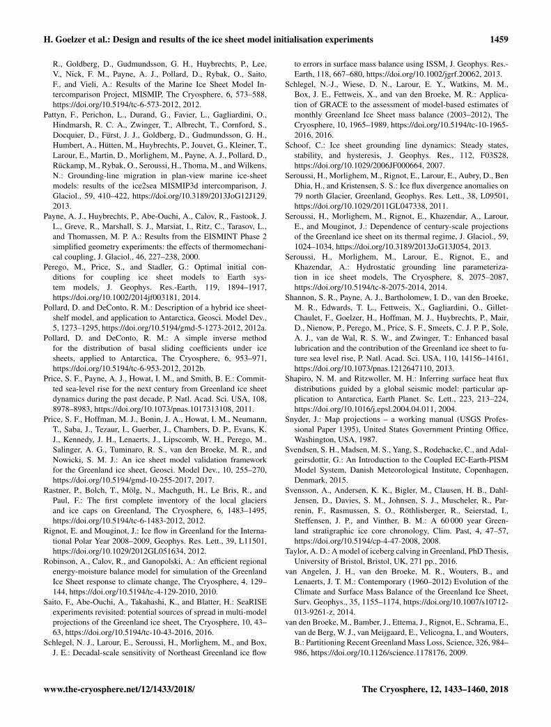
H. Goelzer et al.: Design and results of the ice sheet model initialisation experiments 1459
R., Goldberg, D., Gudmundsson, G. H., Huybrechts, P., Lee,V., Nick, F. M., Payne, A. J., Pollard, D., Rybak, O., Saito,F., and Vieli, A.: Results of the Marine Ice Sheet Model In-tercomparison Project, MISMIP, The Cryosphere, 6, 573–588,https://doi.org/10.5194/tc-6-573-2012, 2012.
Pattyn, F., Perichon, L., Durand, G., Favier, L., Gagliardini, O.,Hindmarsh, R. C. A., Zwinger, T., Albrecht, T., Cornford, S.,Docquier, D., Fürst, J. J., Goldberg, D., Gudmundsson, G. H.,Humbert, A., Hütten, M., Huybrechts, P., Jouvet, G., Kleiner, T.,Larour, E., Martin, D., Morlighem, M., Payne, A. J., Pollard, D.,Rückamp, M., Rybak, O., Seroussi, H., Thoma, M., and Wilkens,N.: Grounding-line migration in plan-view marine ice-sheetmodels: results of the ice2sea MISMIP3d intercomparison, J.Glaciol., 59, 410–422, https://doi.org/10.3189/2013JoG12J129,2013.
Payne, A. J., Huybrechts, P., Abe-Ouchi, A., Calov, R., Fastook, J.L., Greve, R., Marshall, S. J., Marsiat, I., Ritz, C., Tarasov, L.,and Thomassen, M. P. A.: Results from the EISMINT Phase 2simplified geometry experiments: the effects of thermomechani-cal coupling, J. Glaciol., 46, 227–238, 2000.
Perego, M., Price, S., and Stadler, G.: Optimal initial con-ditions for coupling ice sheet models to Earth sys-tem models, J. Geophys. Res.-Earth, 119, 1894–1917,https://doi.org/10.1002/2014jf003181, 2014.
Pollard, D. and DeConto, R. M.: Description of a hybrid ice sheet-shelf model, and application to Antarctica, Geosci. Model Dev.,5, 1273–1295, https://doi.org/10.5194/gmd-5-1273-2012, 2012a.
Pollard, D. and DeConto, R. M.: A simple inverse methodfor the distribution of basal sliding coefficients under icesheets, applied to Antarctica, The Cryosphere, 6, 953–971,https://doi.org/10.5194/tc-6-953-2012, 2012b.
Price, S. F., Payne, A. J., Howat, I. M., and Smith, B. E.: Commit-ted sea-level rise for the next century from Greenland ice sheetdynamics during the past decade, P. Natl. Acad. Sci. USA, 108,8978–8983, https://doi.org/10.1073/pnas.1017313108, 2011.
Price, S. F., Hoffman, M. J., Bonin, J. A., Howat, I. M., Neumann,T., Saba, J., Tezaur, I., Guerber, J., Chambers, D. P., Evans, K.J., Kennedy, J. H., Lenaerts, J., Lipscomb, W. H., Perego, M.,Salinger, A. G., Tuminaro, R. S., van den Broeke, M. R., andNowicki, S. M. J.: An ice sheet model validation frameworkfor the Greenland ice sheet, Geosci. Model Dev., 10, 255–270,https://doi.org/10.5194/gmd-10-255-2017, 2017.
Rastner, P., Bolch, T., Mölg, N., Machguth, H., Le Bris, R., andPaul, F.: The first complete inventory of the local glaciersand ice caps on Greenland, The Cryosphere, 6, 1483–1495,https://doi.org/10.5194/tc-6-1483-2012, 2012.
Rignot, E. and Mouginot, J.: Ice flow in Greenland for the Interna-tional Polar Year 2008–2009, Geophys. Res. Lett., 39, L11501,https://doi.org/10.1029/2012GL051634, 2012.
Robinson, A., Calov, R., and Ganopolski, A.: An efficient regionalenergy-moisture balance model for simulation of the GreenlandIce Sheet response to climate change, The Cryosphere, 4, 129–144, https://doi.org/10.5194/tc-4-129-2010, 2010.
Saito, F., Abe-Ouchi, A., Takahashi, K., and Blatter, H.: SeaRISEexperiments revisited: potential sources of spread in multi-modelprojections of the Greenland ice sheet, The Cryosphere, 10, 43–63, https://doi.org/10.5194/tc-10-43-2016, 2016.
Schlegel, N. J., Larour, E., Seroussi, H., Morlighem, M., and Box,J. E.: Decadal-scale sensitivity of Northeast Greenland ice flow
to errors in surface mass balance using ISSM, J. Geophys. Res.-Earth, 118, 667–680, https://doi.org/10.1002/jgrf.20062, 2013.
Schlegel, N.-J., Wiese, D. N., Larour, E. Y., Watkins, M. M.,Box, J. E., Fettweis, X., and van den Broeke, M. R.: Applica-tion of GRACE to the assessment of model-based estimates ofmonthly Greenland Ice Sheet mass balance (2003–2012), TheCryosphere, 10, 1965–1989, https://doi.org/10.5194/tc-10-1965-2016, 2016.
Schoof, C.: Ice sheet grounding line dynamics: Steady states,stability, and hysteresis, J. Geophys. Res., 112, F03S28,https://doi.org/10.1029/2006JF000664, 2007.
Seroussi, H., Morlighem, M., Rignot, E., Larour, E., Aubry, D., BenDhia, H., and Kristensen, S. S.: Ice flux divergence anomalies on79 north Glacier, Greenland, Geophys. Res. Lett., 38, L09501,https://doi.org/10.1029/2011GL047338, 2011.
Seroussi, H., Morlighem, M., Rignot, E., Khazendar, A., Larour,E., and Mouginot, J.: Dependence of century-scale projectionsof the Greenland ice sheet on its thermal regime, J. Glaciol., 59,1024–1034, https://doi.org/10.3189/2013JoG13J054, 2013.
Seroussi, H., Morlighem, M., Larour, E., Rignot, E., andKhazendar, A.: Hydrostatic grounding line parameteriza-tion in ice sheet models, The Cryosphere, 8, 2075–2087,https://doi.org/10.5194/tc-8-2075-2014, 2014.
Shannon, S. R., Payne, A. J., Bartholomew, I. D., van den Broeke,M. R., Edwards, T. L., Fettweis, X., Gagliardini, O., Gillet-Chaulet, F., Goelzer, H., Hoffman, M. J., Huybrechts, P., Mair,D., Nienow, P., Perego, M., Price, S. F., Smeets, C. J. P. P., Sole,A. J., van de Wal, R. S. W., and Zwinger, T.: Enhanced basallubrication and the contribution of the Greenland ice sheet to fu-ture sea level rise, P. Natl. Acad. Sci. USA, 110, 14156–14161,https://doi.org/10.1073/pnas.1212647110, 2013.
Shapiro, N. M. and Ritzwoller, M. H.: Inferring surface heat fluxdistributions guided by a global seismic model: particular ap-plication to Antarctica, Earth Planet. Sc. Lett., 223, 213–224,https://doi.org/10.1016/j.epsl.2004.04.011, 2004.
Snyder, J.: Map projections – a working manual (USGS Profes-sional Paper 1395), United States Government Printing Office,Washington, USA, 1987.
Svendsen, S. H., Madsen, M. S., Yang, S., Rodehacke, C., and Adal-geirsdottir, G.: An Introduction to the Coupled EC-Earth-PISMModel System, Danish Meteorological Institute, Copenhagen,Denmark, 2015.
Svensson, A., Andersen, K. K., Bigler, M., Clausen, H. B., Dahl-Jensen, D., Davies, S. M., Johnsen, S. J., Muscheler, R., Par-renin, F., Rasmussen, S. O., Röthlisberger, R., Seierstad, I.,Steffensen, J. P., and Vinther, B. M.: A 60 000 year Green-land stratigraphic ice core chronology, Clim. Past, 4, 47–57,https://doi.org/10.5194/cp-4-47-2008, 2008.
Taylor, A. D.: A model of iceberg calving in Greenland, PhD Thesis,University of Bristol, Bristol, UK, 271 pp., 2016.
van Angelen, J. H., van den Broeke, M. R., Wouters, B., andLenaerts, J. T. M.: Contemporary (1960–2012) Evolution of theClimate and Surface Mass Balance of the Greenland Ice Sheet,Surv. Geophys., 35, 1155–1174, https://doi.org/10.1007/s10712-013-9261-z, 2014.
van den Broeke, M., Bamber, J., Ettema, J., Rignot, E., Schrama, E.,van de Berg, W. J., van Meijgaard, E., Velicogna, I., and Wouters,B.: Partitioning Recent Greenland Mass Loss, Science, 326, 984–986, https://doi.org/10.1126/science.1178176, 2009.
www.the-cryosphere.net/12/1433/2018/ The Cryosphere, 12, 1433–1460, 2018

1460 H. Goelzer et al.: Design and results of the ice sheet model initialisation experiments
Velicogna, I., Sutterley, T. C., and van den Broeke, M. R.: Regionalacceleration in ice mass loss from Greenland and Antarctica us-ing GRACE time-variable gravity data, Geophys. Res. Lett., 41,8130–8137, https://doi.org/10.1002/2014GL061052, 2014.
Vizcaino, M., Mikolajewicz, U., Ziemen, F., Rodehacke, C.B., Greve, R., and van den Broeke, M. R.: Coupledsimulations of Greenland Ice Sheet and climate changeup to A.D. 2300, Geophys. Res. Lett., 42, 3927–3935,https://doi.org/10.1002/2014GL061142, 2015.
The Cryosphere, 12, 1433–1460, 2018 www.the-cryosphere.net/12/1433/2018/