11 Gewöhnliche Differentialgleichung

11.1 Einleitung und Grundbegriffe

Def.: Eine gewöhnliche Differentialgleichung ist eine

Funktionsgleichung,

die eine unbekannte Funktion y = y (x)sowie deren Ableitungen nach x enthält.Die Ordnung der Differentialgleichung ist die Ordnung der höchsten vorkommenden Ableitung von y (x) nach x.

Die allgemeine Differentialgleichung n-ter Ornung für eine Funktion y = y (x) :

( )F x y y y y n, , , ,....., ( )′ ′′ = 0 implizite Form

( )y f x y y y yn n( ) ( ), , , ,.....,= ′ ′′ −1 explizite Form

Als Lösung (Lösungsfunktion, Integral) einer Differentialgleichungbezeichnet man jede Funktion

y = y (x) ,

die samt ihren Ableitungen in die Differentialgleichung eingesetzt,diese identisch erfüllt.

Beispiele:

′ =y x2 explizite DGL 1. Ordnung (y’)

x y y+ ⋅ ′ = 0 implizite DGL 1. Ordnung (y’)

′ + ⋅ ′′ =y y y 0 implizite DGL 2. Ordnung (y’’)

′′′ + ⋅ ′ =y y x2 cos implizite DGL 3. Ordnung (y’’’)

y y y ex( ) ( )6 4− + ′′ = implizite DGL 6. Ordnung (y(6))

Man unterscheidet folgende Typen von Lösungen:

1. Die allgemeine Lösung einer DGL n-ter Ordnung; sieenthält noch n unbestimmte und voneinander unabhängige n-Konstanten

y = y (x, C1, C2, ....., Cn)

2. Eine spezielle (partikuläre) Lösung wird aus derallgemeinen Lösung gewonnen, indem man aufgrund zusätzlicher Bedingungen den n-Konstanten feste Werte zuweist. Dies kann beispielsweise durch Anfangs- oder Randbedingungen geschehen.

11.2 Geometrische Deutung

′ = ⋅y x2

Lösung durch Integration:

′ = ⋅ = +∫∫ y dx x dx x C2 2

allg. Lösung: y = x2 + C Parabelschar

Die partikuläre Lösung entsteht für jeden speziellen Wert desParameters C.

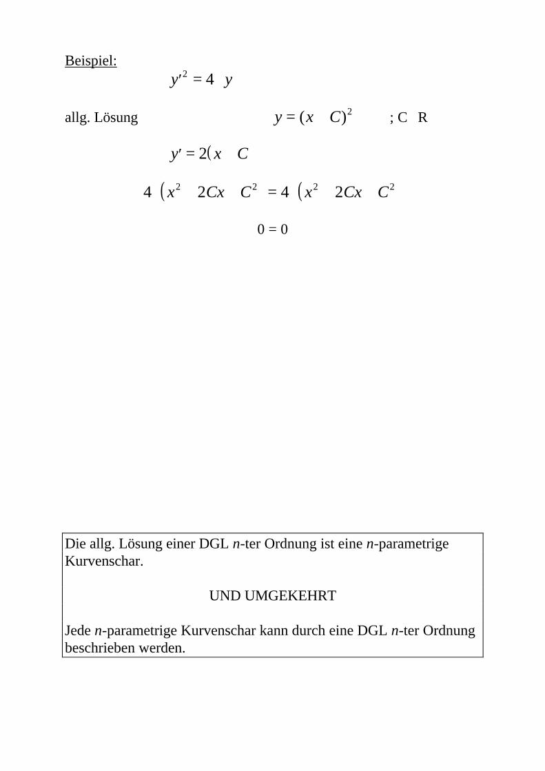
Beispiel:′ = ⋅y y2 4

allg. Lösung ⇒ y x C= +( )2 ; C∈R

( )′ = +y x C2

( ) ( )4 2 4 22 2 2 2⋅ + + = ⋅ + +x Cx C x Cx C

0 = 0

Die allg. Lösung einer DGL n-ter Ordnung ist eine n-parametrigeKurvenschar.

UND UMGEKEHRT

Jede n-parametrige Kurvenschar kann durch eine DGL n-ter Ordnungbeschrieben werden.

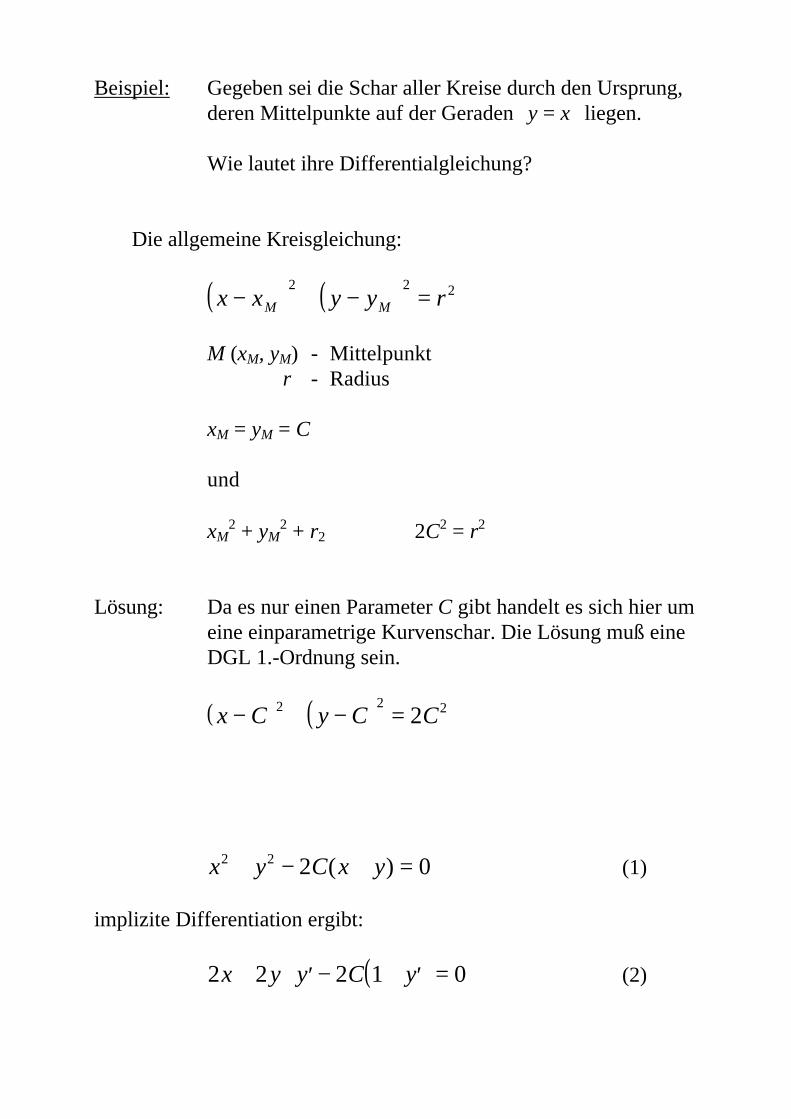
Beispiel: Gegeben sei die Schar aller Kreise durch den Ursprung,deren Mittelpunkte auf der Geraden y = x liegen.

Wie lautet ihre Differentialgleichung?

Die allgemeine Kreisgleichung:

( ) ( )x x y y rM M− + − =2 2 2

M (xM, yM) - Mittelpunktr - Radius

xM = yM = C

und

xM2 + yM

2 + r2 ⇒ 2C2 = r2

Lösung: Da es nur einen Parameter C gibt handelt es sich hier umeine einparametrige Kurvenschar. Die Lösung muß eine DGL 1.-Ordnung sein.

( ) ( )x C y C C− + − =⋅⋅⋅

2 2 22

x y C x y2 2 2 0+ − + =( ) (1)

implizite Differentiation ergibt:

( )2 2 2 1 0x y y C y+ ⋅ ′ − + ′ = (2)

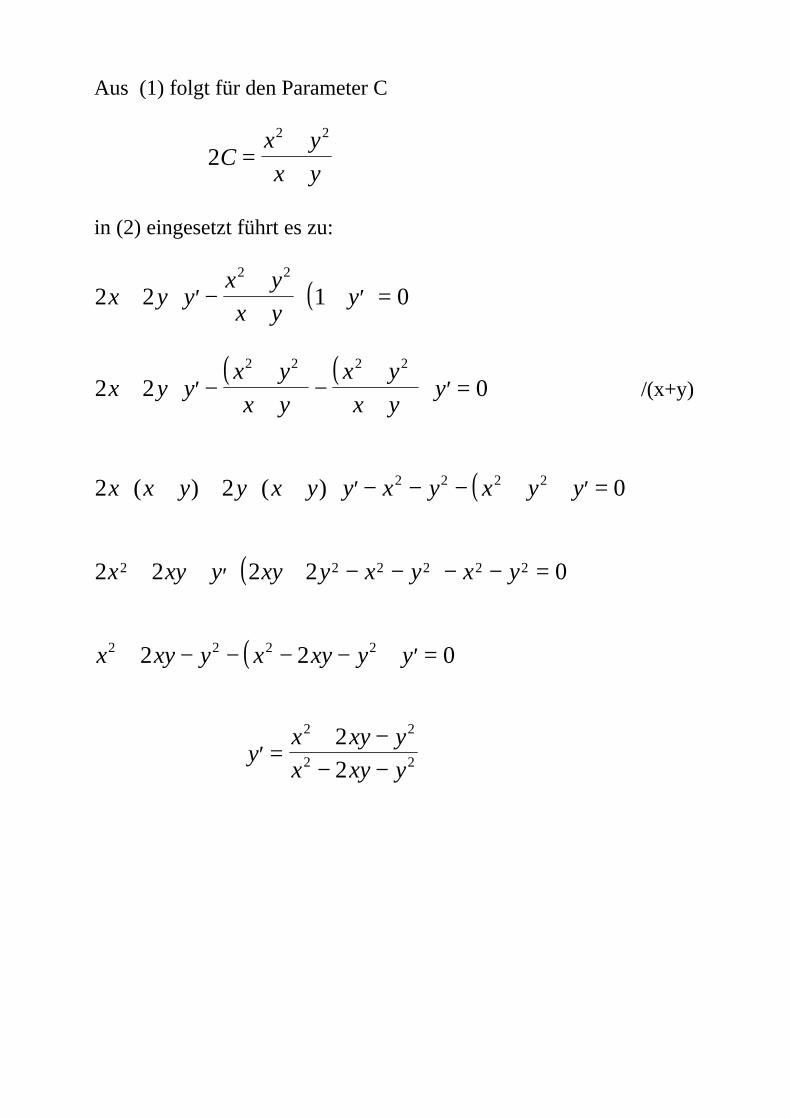
Aus (1) folgt für den Parameter C

22 2

Cx y

x y=

++

in (2) eingesetzt führt es zu:

( )2 2 1 02 2

x y yx y

x yy+ ⋅ ′ −

++

⋅ + ′ =

( ) ( )2 2 0

2 2 2 2

x y yx y

x y

x y

x yy+ ⋅ ′ −

++

−++

⋅ ′ = /(x+y)

( )2 2 02 2 2 2x x y y x y y x y x y y⋅ + + ⋅ + ⋅ ′ − − − + ⋅ ′ =( ) ( )

( )2 2 2 2 02 2 2 2 2 2x xy y xy y x y x y+ + ′ ⋅ + − − − − =

( )x xy y x xy y y2 2 2 22 2 0+ − − − − ⋅ ′ =

′ =+ −− −

yx xy y

x xy y

2 2

2 2

22

11.3 Anfangswert- und Randwertprobleme

11.4 Differentialgleichungen erster Ordnung

Lösungsmethoden

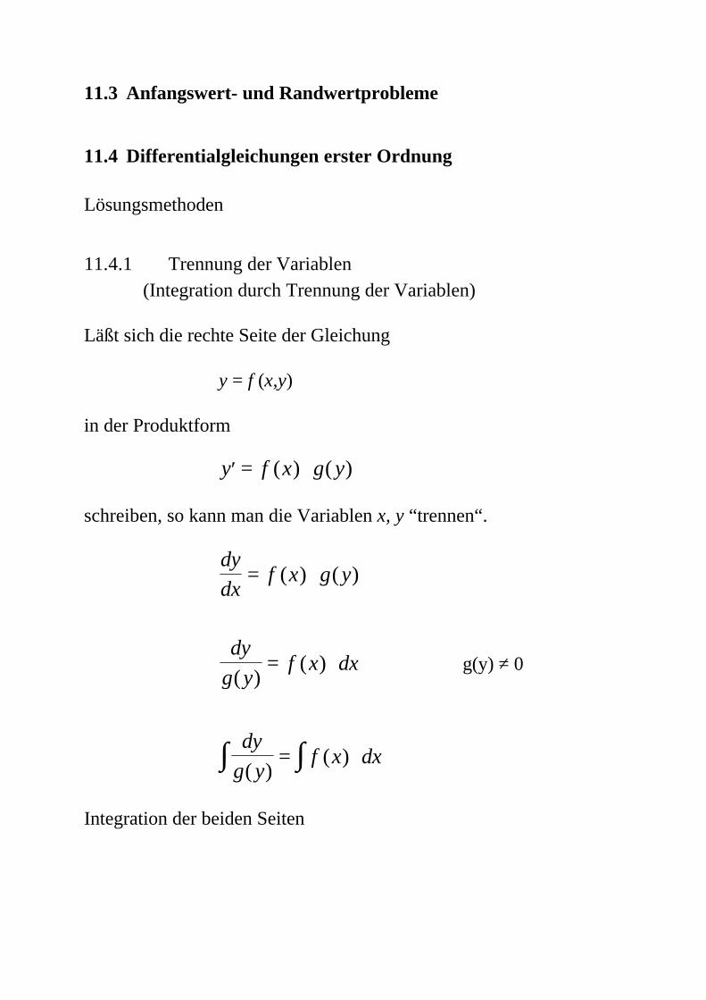
11.4.1 Trennung der Variablen(Integration durch Trennung der Variablen)

Läßt sich die rechte Seite der Gleichung

y = f (x,y)

in der Produktform

′ = ⋅y f x g y( ) ( )

schreiben, so kann man die Variablen x, y “trennen“.

dy

dxf x g y

dy

g yf x dx

dy

g yf x dx

= ⋅

= ⋅

= ⋅∫ ∫

( ) ( )

( )( )

( )( )

g(y) ≠ 0

Integration der beiden Seiten

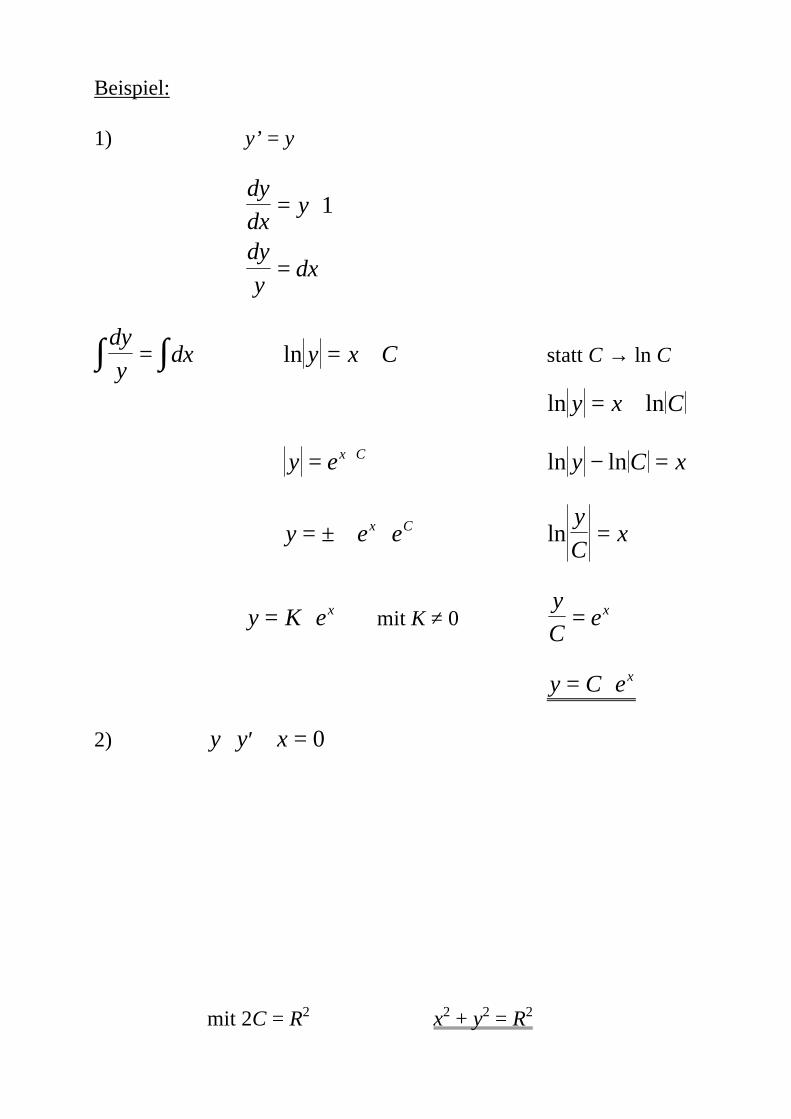
Beispiel:

1) y’ = y

dy

dxy

dy

ydx

= ⋅

=

1

dy

ydx∫ ∫= ⇒ ln y x C= + statt C → ln C

⇓ ln lny x C= +

y ex C= + ln lny C x− =

y e ex C= ± ⋅ lny

Cx=

y K ex= ⋅ mit K ≠ 0y

Cex=

y C ex= ⋅

2) y y x⋅ ′ + = 0

mit 2C = R2 x2 + y2 = R2

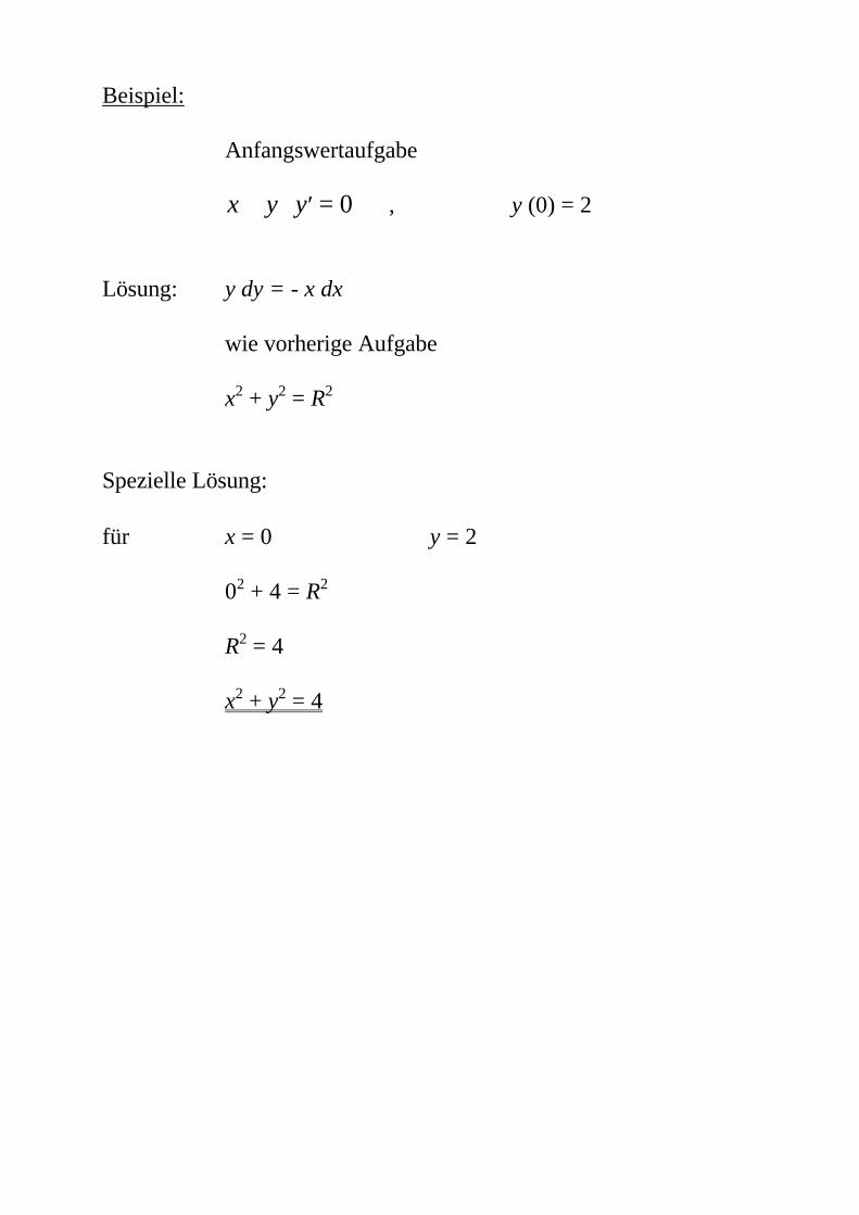
Beispiel:

Anfangswertaufgabe

x y y+ ⋅ ′ = 0 , y (0) = 2

Lösung: y dy = - x dx

wie vorherige Aufgabe

x2 + y2 = R2

Spezielle Lösung:

für x = 0 ⇒ y = 2

02 + 4 = R2

R2 = 4

x2 + y2 = 4

11.4.2 Integration einer Differentialgleichung durch SubstitutionHomogene Differentialgleichungen

Eine explizite DGL 1. Ordnung

y’ = f (x,y)

kann mit Hilfe einer geeigneten Substitution auf eine separableDgl. 1. Ordnung zurückgeführt werden.

11.4.2.1 DGL vom Typ y’ = f (ax + by + c)

Substitution: u = ax + by + c (1)

Dabei sind y und u als Funktionen von x zu betrachten.

Durch Differentiation der Substitution nach x erhalten wir:

u’ = a + by’ (2)

Durch die Substitution ergibt sich: y’ = f (u)

Damit ist aus (2) eine separable DGL

u’ = a + b f (u)

entstanden, die durch Trennung der Variablen gelöst werden kann, dadie rechte Seite dieser Gleichung nur von u abhängt.Anschließend führen wir die Rücksubstitution durch.

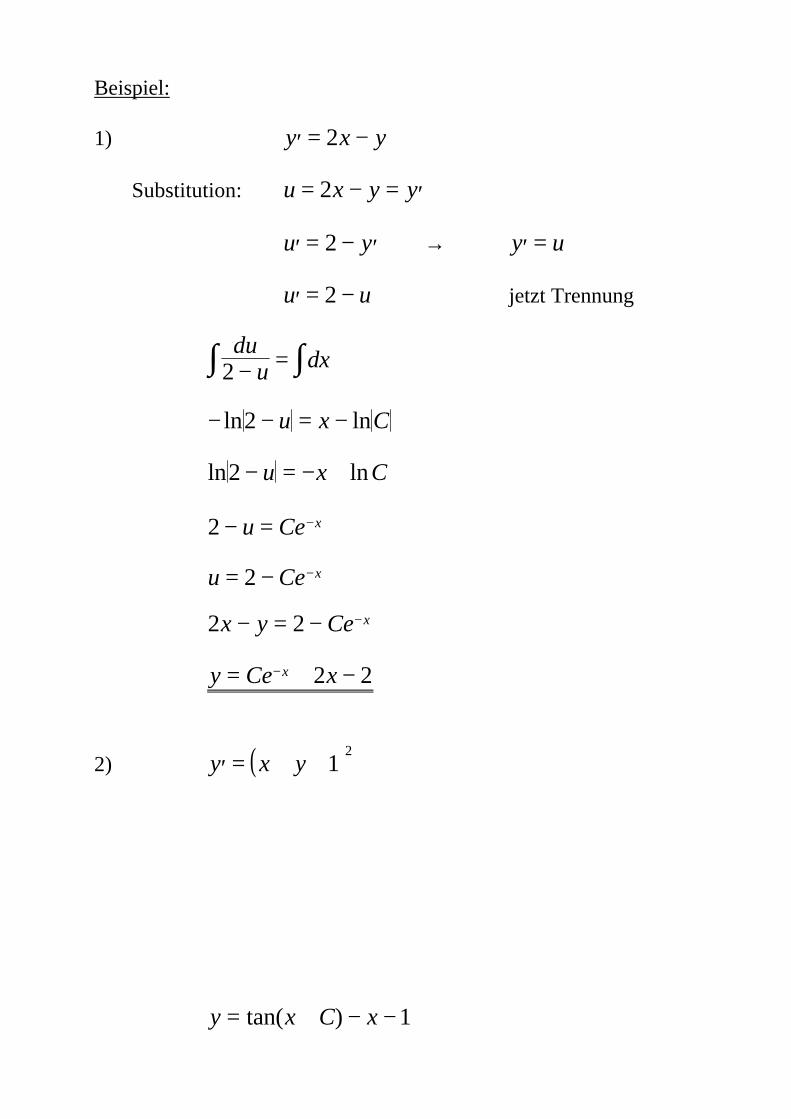
Beispiel:

1) ′ = −y x y2

Substitution: u x y y= − = ′2

′ = − ′u y2 → ′ =y u

′ = −u u2 jetzt Trennung

duu dx2 − =∫ ∫

− − = −ln ln2 u x C

ln ln2 − = − +u x C

2 − = −u Ce x

u Ce x= − −2

2 2x y Ce x− = − −

y Ce xx= + −− 2 2

2) ( )′ = + +y x y 12

y x C x= + − −tan( ) 1

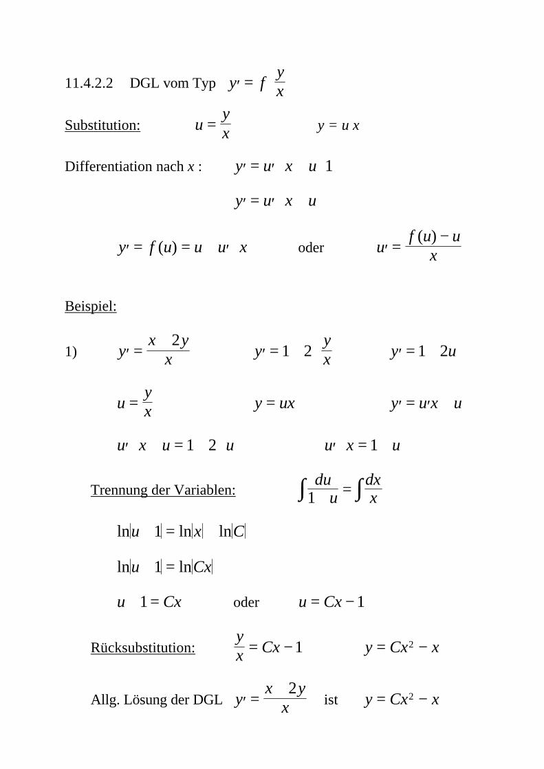
11.4.2.2 DGL vom Typ ′ =

y f

yx

Substitution: uyx= ⇒ y = u x

Differentiation nach x : ′ = ′ ⋅ + ⋅y u x u 1

′ = ′ ⋅ +y u x u

′ = = + ′ ⋅y f u u u x( ) oder ′ =−

uf u u

x( )

Beispiel:

1) ′ =+

yx y

x2

⇒ ′ = + ⋅yyx1 2 ⇒ ′ = +y u1 2

uyx= ⇒ y ux= ⇒ ′ = ′ +y u x u

′ ⋅ + = + ⋅u x u u1 2 ⇒ ′ ⋅ = +u x u1

Trennung der Variablen:du

udxx1+ =∫ ∫

ln ln lnu x C+ = +1

ln lnu Cx+ =1

u Cx+ =1 oder u Cx= − 1

Rücksubstitution:yx Cx= − 1 ⇒ y Cx x= −2

Allg. Lösung der DGL ′ =+

yx y

x2

ist y Cx x= −2

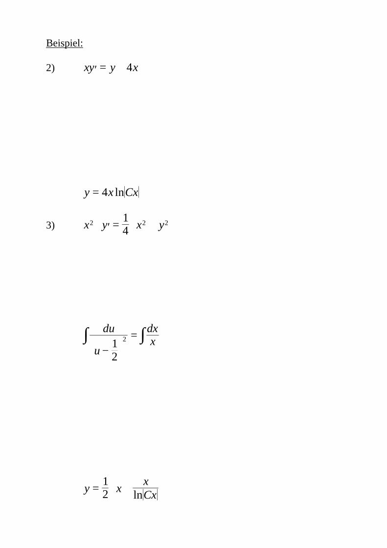
Beispiel:

2) xy y x′ = + 4

y x Cx= 4 ln

3) x y x y2 2 214⋅ ′ = ⋅ +

du

u

dxx

−

=∫ ∫12

2

y xxCx

= ⋅ +12 ln

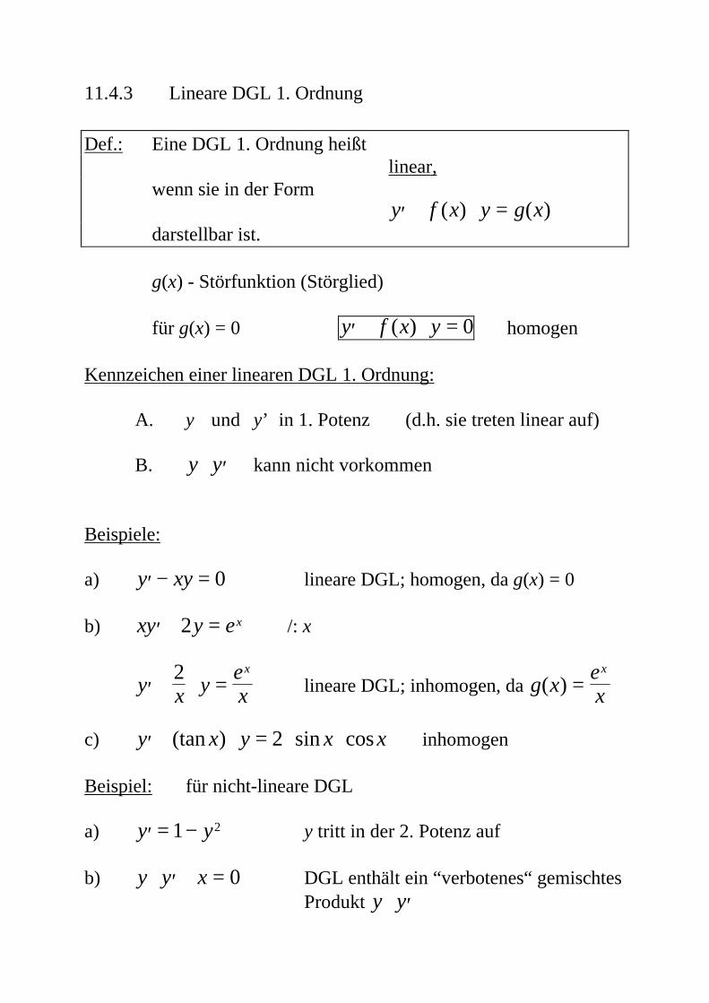
11.4.3 Lineare DGL 1. Ordnung

Def.: Eine DGL 1. Ordnung heißtlinear,

wenn sie in der Form′ + ⋅ =y f x y g x( ) ( )

darstellbar ist.

g(x) - Störfunktion (Störglied)

für g(x) = 0 ⇒ ′ + ⋅ =y f x y( ) 0 homogen

Kennzeichen einer linearen DGL 1. Ordnung:

A. y und y’ in 1. Potenz (d.h. sie treten linear auf)

B. y y⋅ ′ kann nicht vorkommen

Beispiele:

a) ′ − =y xy 0 lineare DGL; homogen, da g(x) = 0

b) xy y ex′ + =2 /: x

′ + ⋅ =y x yex

x2lineare DGL; inhomogen, da g x

ex

x

( ) =

c) ′ + ⋅ = ⋅ ⋅y x y x x(tan ) sin cos2 inhomogen

Beispiel: für nicht-lineare DGL

a) ′ = −y y1 2 y tritt in der 2. Potenz auf

b) y y x⋅ ′ + = 0 DGL enthält ein “verbotenes“ gemischtesProdukt y y⋅ ′

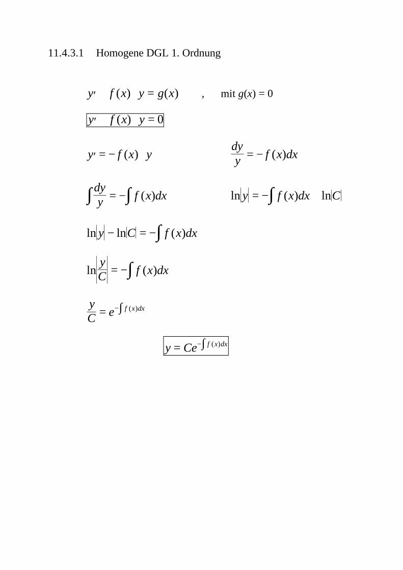
11.4.3.1 Homogene DGL 1. Ordnung

′ + ⋅ =y f x y g x( ) ( ) , mit g(x) = 0

′ + ⋅ =y f x y( ) 0

′ = − ⋅y f x y( ) ⇒dyy f x dx= − ( )

dyy f x dx= −∫∫ ( ) ⇒ ln ( ) lny f x dx C= − +∫

ln ln ( )y C f x dx− = −∫

ln ( )yC f x dx= −∫

yC e f x dx= ∫− ( )

y Ce f x dx= ∫− ( )

Beispiel:

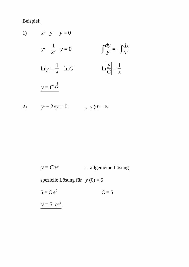
1) x y y2 0⋅ ′ + =

′ + ⋅ =y x y1

02 ⇒dyy

dxx∫ ∫= − 2

ln lny x C= +1⇒ ln

yC x= 1

y Ce x=1

2) ′ − =y xy2 0 , y (0) = 5

y Cex= 2 - allgemeine Lösung

spezielle Lösung für y (0) = 5

5 = C e0 ⇒ C = 5

y ex= ⋅5 2

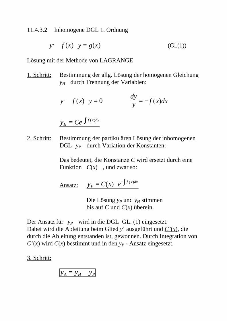
11.4.3.2 Inhomogene DGL 1. Ordnung

′ + ⋅ =y f x y g x( ) ( ) (Gl.(1))

Lösung mit der Methode von LAGRANGE

1. Schritt: Bestimmung der allg. Lösung der homogenen Gleichung yH durch Trennung der Variablen:

′ + ⋅ =y f x y( ) 0 ⇒dyy f x dx= − ( )

y CeHf x dx= ∫− ( )

2. Schritt: Bestimmung der partikulären Lösung der inhomogenen DGL yP durch Variation der Konstanten:

Das bedeutet, die Konstanze C wird ersetzt durch eine Funktion C(x) , und zwar so:

Ansatz: y C x ePf x dx= ⋅ ∫−( ) ( )

Die Lösung yP und yH stimmenbis auf C und C(x) überein.

Der Ansatz für yP wird in die DGL GL. (1) eingesetzt.Dabei wird die Ableitung beim Glied y’ ausgeführt und C’(x), diedurch die Ableitung entstanden ist, gewonnen. Durch Integration vonC’(x) wird C(x) bestimmt und in den yP - Ansatz eingesetzt.

3. Schritt:

y y yA H P= +

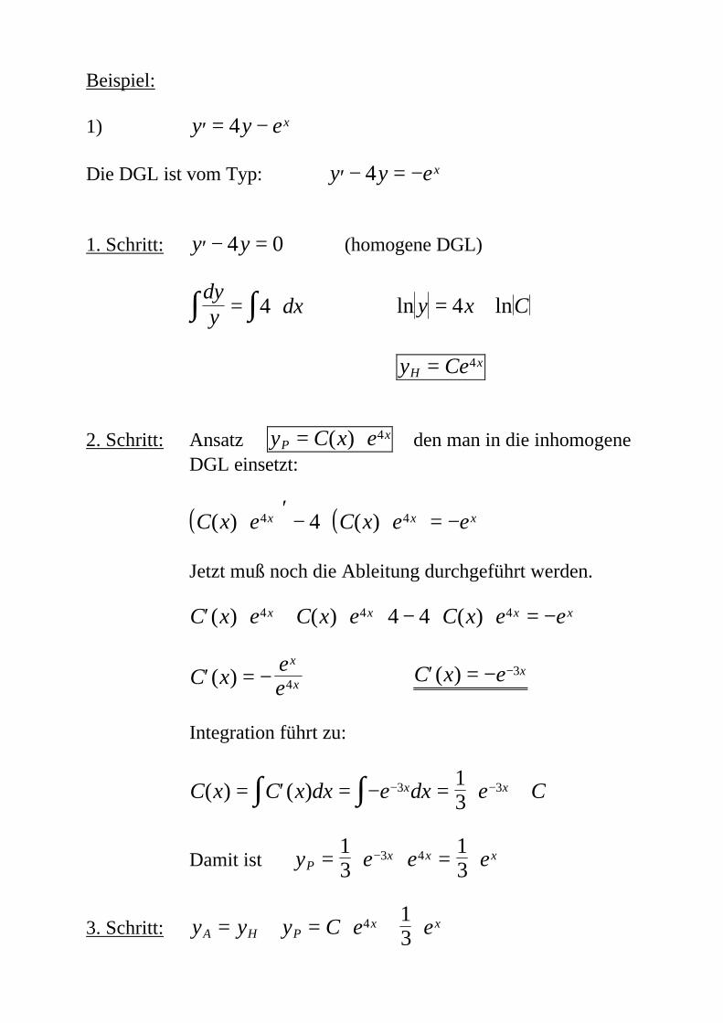
Beispiel:

1) ′ = −y y ex4

Die DGL ist vom Typ: ′ − = −y y ex4

1. Schritt: ′ − =y y4 0 (homogene DGL)

dyy dx∫ ∫= ⋅4 ⇒ ln lny x C= +4

⇒ y CeHx= 4

2. Schritt: Ansatz y C x ePx= ⋅( ) 4 den man in die inhomogene

DGL einsetzt:

( ) ( )C x e C x e ex x x( ) ( )⋅′− ⋅ ⋅ = −4 44

Jetzt muß noch die Ableitung durchgeführt werden.

C x e C x e C x e ex x x x′ ⋅ + ⋅ ⋅ − ⋅ ⋅ = −( ) ( ) ( )4 4 44 4

C xee

x

x′ = −( ) 4 ⇒ C x e x′ = − −( ) 3

Integration führt zu:

C x C x dx e dx e Cx x( ) ( )= ′ = − = ⋅ +− −∫∫ 3 313

Damit ist y e e ePx x x= ⋅ ⋅ = ⋅−1

313

3 4

3. Schritt: y y y C e eA H Px x= + = ⋅ + ⋅4 1

3

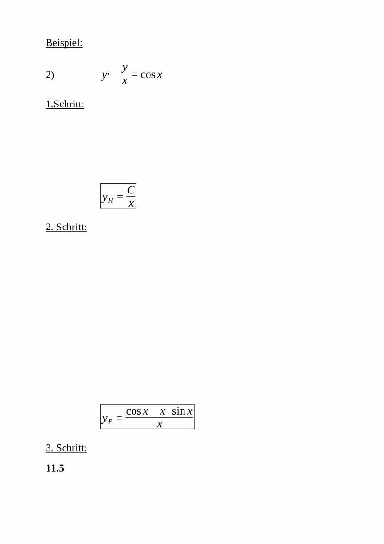
Beispiel:

2) ′ + =yyx xcos

1.Schritt:

yCxH =

2. Schritt:

yx x x

xP = + ⋅cos sin

3. Schritt:

11.5

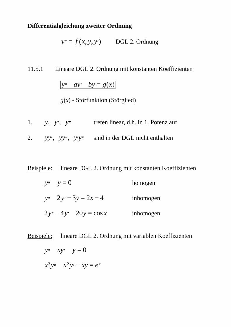
Differentialgleichung zweiter Ordnung

′′ = ′y f x y y( , , ) DGL 2. Ordnung

11.5.1 Lineare DGL 2. Ordnung mit konstanten Koeffizienten

′′ + ′ + =y ay by g x( )

g(x) - Störfunktion (Störglied)

1. y y y, ,′ ′′ treten linear, d.h. in 1. Potenz auf

2. yy yy y y′ ′′ ′ ′′, , sind in der DGL nicht enthalten

Beispiele: lineare DGL 2. Ordnung mit konstanten Koeffizienten

′′ + =y y 0 homogen

′′ + ′ − = −y y y x2 3 2 4 inhomogen

2 4 20′′ − ′ + =y y y xcos inhomogen

Beispiele: lineare DGL 2. Ordnung mit variablen Koeffizienten

′′ + ′ + =y xy y 0

x y x y xy ex3 2′′ + ′ − =

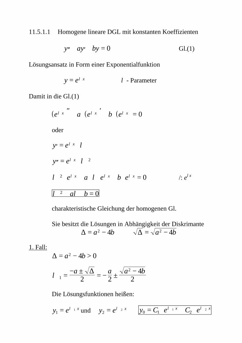
11.5.1.1 Homogene lineare DGL mit konstanten Koeffizienten

′′ + ′ + =y ay by 0 Gl.(1)

Lösungsansatz in Form einer Exponentialfunktion

y e x= ⋅λ λ - Parameter

Damit in die Gl.(1)

( ) ( ) ( )e a e b ex x xλ λ λ⋅ ⋅ ⋅″ + ⋅ ′ + ⋅ = 0

oder

′ = ⋅⋅y e xλ λ

′′ = ⋅⋅y e xλ λ 2

λ λλ λ λ2 0⋅ + ⋅ ⋅ + ⋅ =⋅ ⋅ ⋅e a e b ex x x /: eλx

λ λ2 0+ + =a b

charakteristische Gleichung der homogenen Gl.

Sie besitzt die Lösungen in Abhängigkeit der Diskrimante∆ = −a b2 4 ∆ = −a b2 4

1. Fall:∆ = − >a b2 4 0

λ 1

2

2 24

2= − ± = − ± −a a a b∆

Die Lösungsfunktionen heißen:

y e x1

1= ⋅λ und y e x2

2= ⋅λ y C e C ex x0 1 2

1 2= ⋅ + ⋅⋅ ⋅λ λ

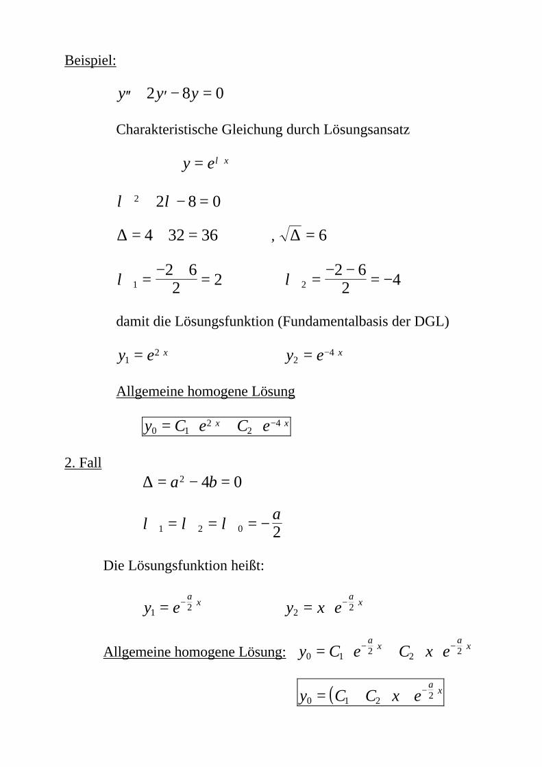
Beispiel:

′′ + ′ − =y y y2 8 0

Charakteristische Gleichung durch Lösungsansatz

y e x= ⋅λ

λ λ2 2 8 0+ − =

∆ = + =4 32 36 , ∆ = 6

λ 12 62 2= − + = λ 2

2 62 4= − − = −

damit die Lösungsfunktion (Fundamentalbasis der DGL)

y e x1

2= ⋅ y e x2

4= − ⋅

Allgemeine homogene Lösung

y C e C ex x0 1

22

4= ⋅ + ⋅⋅ − ⋅

2. Fall∆ = − =a b2 4 0

λ λ λ1 2 0 2= = = − a

Die Lösungsfunktion heißt:

y ea

x1 2= − ⋅ y x e

ax

2 2= ⋅ − ⋅

Allgemeine homogene Lösung: y C e C x ea

xa

x0 1 2 2 2= ⋅ + ⋅ ⋅− ⋅ − ⋅

( )y C C x ea

x0 1 2 2= + ⋅ ⋅ − ⋅

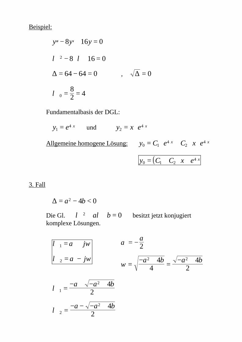
Beispiel:

′′ − ′ + =y y y8 16 0

λ λ2 8 16 0− ⋅ + =

∆ = − =64 64 0 , ∆ = 0

λ 082 4= =

Fundamentalbasis der DGL:

y e x1

4= ⋅ und y x e x2

4= ⋅ ⋅

Allgemeine homogene Lösung: y C e C x ex x0 1

42

4= ⋅ + ⋅ ⋅⋅ ⋅

( )y C C x e x0 1 2

4= + ⋅ ⋅ ⋅

3. Fall

∆ = − <a b2 4 0

Die Gl. λ λ2 0+ + =a b besitzt jetzt konjugiert komplexe Lösungen.

λ α ω

λ α ω

1

2

= +

= −

j

j

α

ω

= −

= − + = − +

a

a b a b

2

44

42

2 2

λ

λ

1

2

2

2

42

42

= − + − +

= − − − +

a a b

a a b

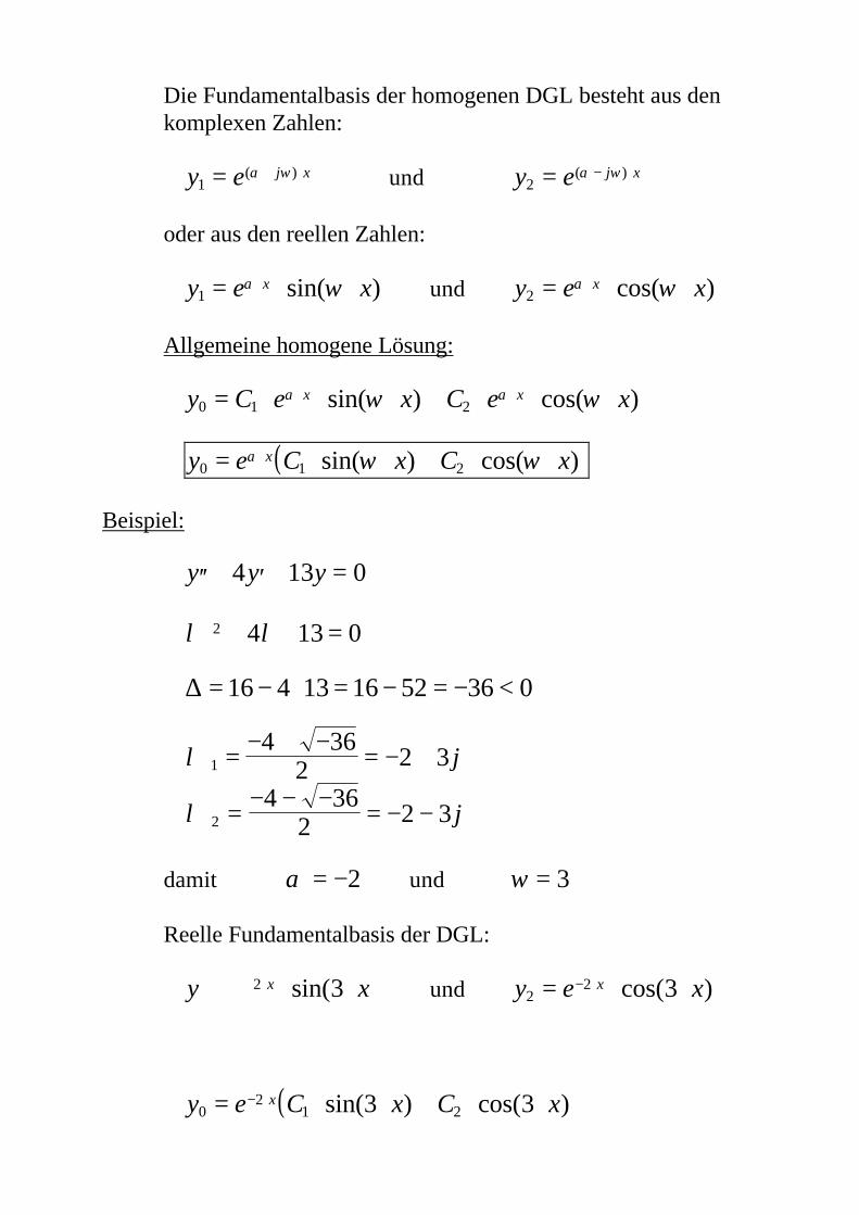
Die Fundamentalbasis der homogenen DGL besteht aus den komplexen Zahlen:

y e j x1 = + ⋅( )α ω und y e j x

2 = − ⋅( )α ω

oder aus den reellen Zahlen:

y e xx1 = ⋅ ⋅⋅α ωsin( ) und y e xx

2 = ⋅ ⋅⋅α ωcos( )

Allgemeine homogene Lösung:

y C e x C e xx x0 1 2= ⋅ ⋅ ⋅ + ⋅ ⋅ ⋅⋅ ⋅α αω ωsin( ) cos( )

( )y e C x C xx0 1 2= ⋅ ⋅ + ⋅ ⋅⋅α ω ωsin( ) cos( )

Beispiel:

′′ + ′ + =y y y4 13 0

λ λ2 4 13 0+ + =

∆ = − ⋅ = − = − <16 4 13 16 52 36 0

λ 14 36

2 2 3= − + − = − + j

λ 24 36

2 2 3= − − − = − − j

damit α = −2 und ω = 3

Reelle Fundamentalbasis der DGL:

y xx2 3⋅ ⋅⋅ sin( und y e xx2

2 3= ⋅ ⋅− ⋅ cos( )

( )y e C x C xx0

21 23 3= ⋅ ⋅ + ⋅ ⋅− ⋅ sin( ) cos( )

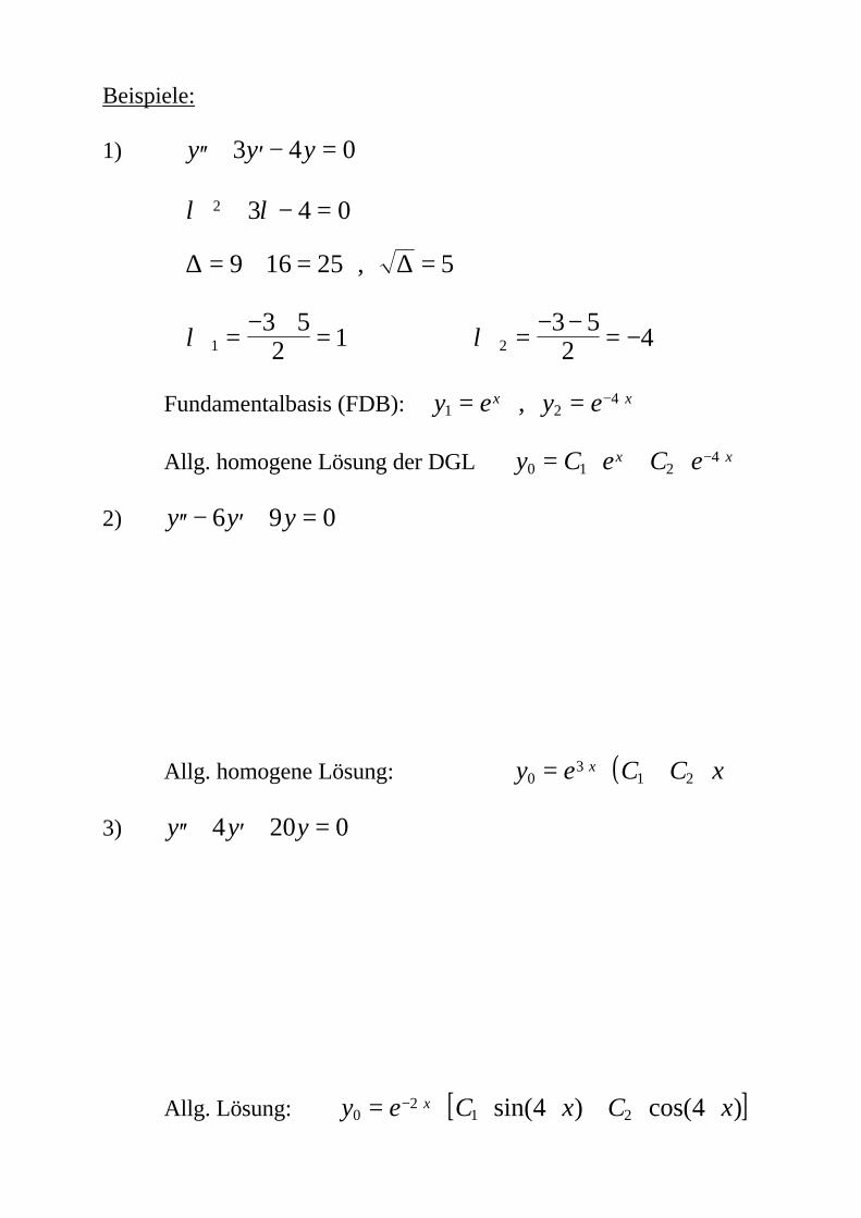
Beispiele:

1) ′′ + ′ − =y y y3 4 0

λ λ2 3 4 0+ − =

∆ ∆= + = =9 16 25 5,

λ 13 52 1= − + = λ 2

3 52 4= − − = −

Fundamentalbasis (FDB): y e y ex x1 2

4= = − ⋅,

Allg. homogene Lösung der DGL y C e C ex x0 1 2

4= ⋅ + ⋅ − ⋅

2) ′′ − ′ + =y y y6 9 0

Allg. homogene Lösung: ( )y e C C xx0

31 2= ⋅ + ⋅⋅

3) ′′ + ′ + =y y y4 20 0

Allg. Lösung: [ ]y e C x C xx0

21 24 4= ⋅ ⋅ ⋅ + ⋅ ⋅− ⋅ sin( ) cos( )

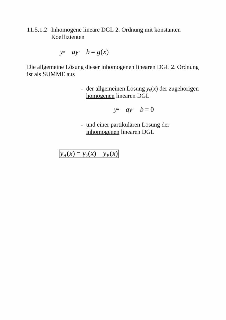
11.5.1.2 Inhomogene lineare DGL 2. Ordnung mit konstanten Koeffizienten

′′ + ′ + =y ay b g x( )

Die allgemeine Lösung dieser inhomogenen linearen DGL 2. Ordnungist als SUMME aus

- der allgemeinen Lösung y0(x) der zugehörigenhomogenen linearen DGL

′′ + ′ + =y ay b 0

- und einer partikulären Lösung derinhomogenen linearen DGL

y x y x y xA P( ) ( ) ( )= +0

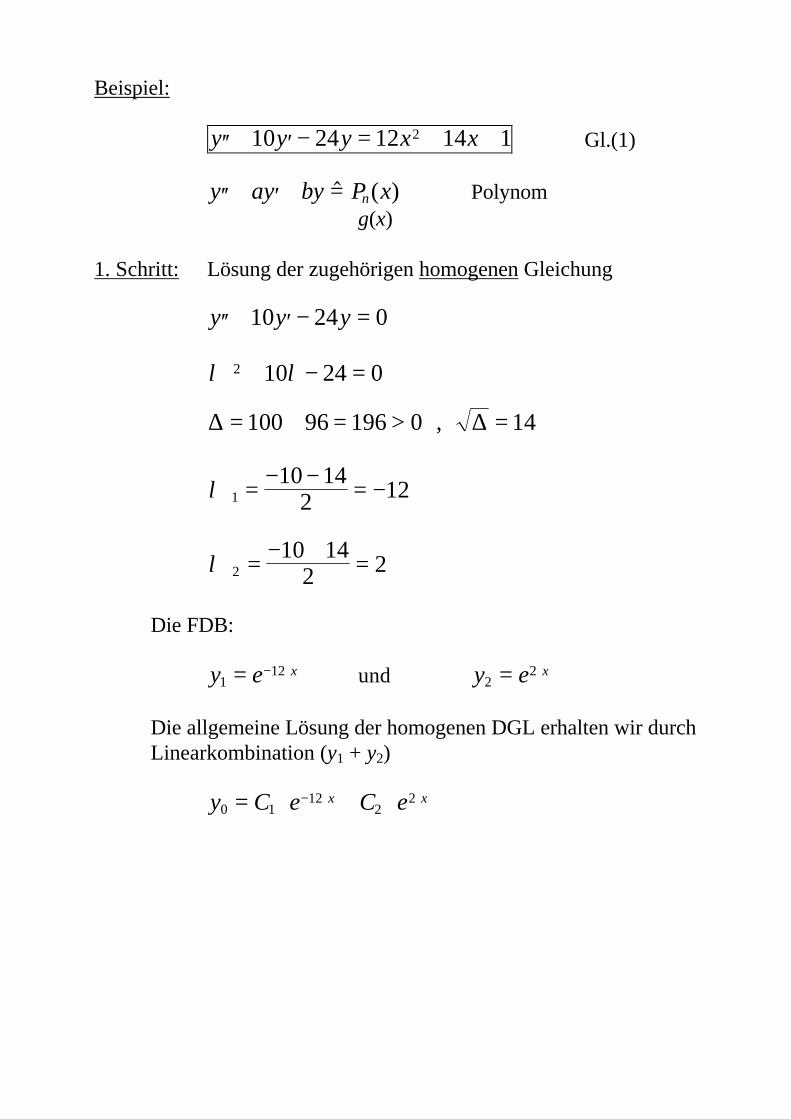
Beispiel:

′′ + ′ − = + +y y y x x10 24 12 14 12 Gl.(1)

′′ + ′ + =y ay by P xn$ ( ) Polynomg(x)

1. Schritt: Lösung der zugehörigen homogenen Gleichung

′′ + ′ − =y y y10 24 0

λ λ2 10 24 0+ − =

∆ ∆= + = > =100 96 196 0 14,

λ 110 14

2 12= − − = −

λ 210 14

2 2= − + =

Die FDB:

y e x1

12= − ⋅ und y e x2

2= ⋅

Die allgemeine Lösung der homogenen DGL erhalten wir durchLinearkombination (y1 + y2)

y C e C ex x0 1

122

2= ⋅ + ⋅− ⋅ ⋅

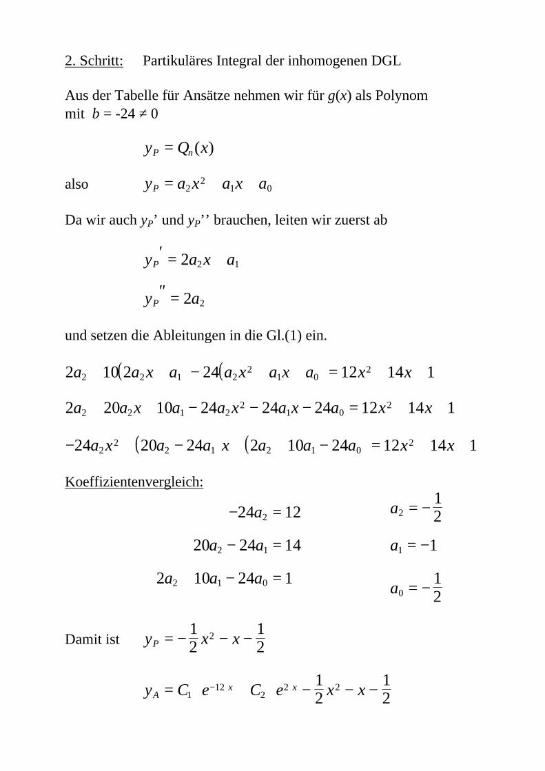
2. Schritt: Partikuläres Integral der inhomogenen DGL

Aus der Tabelle für Ansätze nehmen wir für g(x) als Polynommit b = -24 ≠ 0

y Q xP n= ( )

also y a x a x aP = + +22

1 0

Da wir auch yP’ und yP’’ brauchen, leiten wir zuerst ab

y a x a

y a

P

P

′ = +

″ =

2

2

2 1

2

und setzen die Ableitungen in die Gl.(1) ein.

( ) ( )2 10 2 24 12 14 12 2 1 22

1 02a a x a a x a x a x x+ + − + + = + +

2 20 10 24 24 24 12 14 12 2 1 22

1 02a a x a a x a x a x x+ + − − − = + +

( ) ( )− + − + + − = + +24 20 24 2 10 24 12 14 122

2 1 2 1 02a x a a x a a a x x

Koeffizientenvergleich:

− =

− =

+ − =

24 12

20 24 14

2 10 24 1

2

2 1

2 1 0

a

a a

a a a

⇒

a

a

a

2

1

0

12

1

12

= −

= −

= −

Damit ist y x xP = − − −12

12

2

y C e C e x xAx x= ⋅ + ⋅ − − −− ⋅ ⋅

112

22 21

212

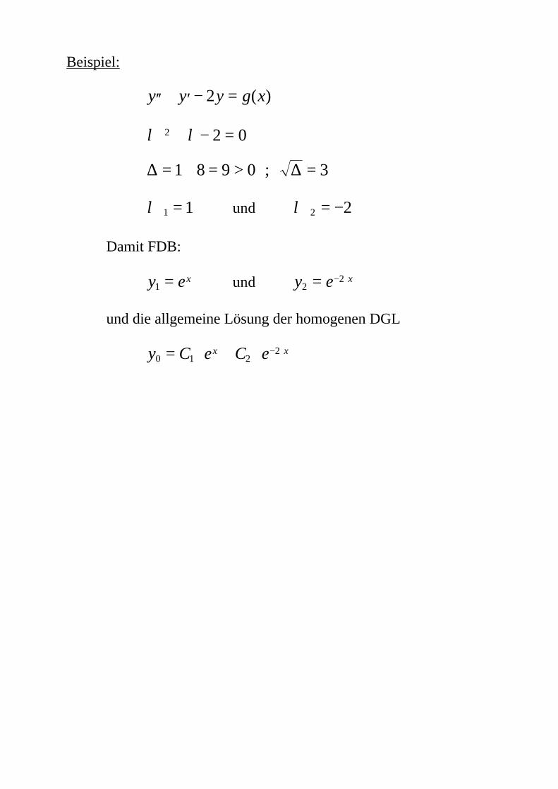
Beispiel:

′′ + ′ − =y y y g x2 ( )

λ λ2 2 0+ − =

∆ ∆= + = > =1 8 9 0 3;

λ 1 1= und λ 2 2= −

Damit FDB:

y ex1 = und y e x

22= − ⋅

und die allgemeine Lösung der homogenen DGL

y C e C ex x0 1 2

2= ⋅ + ⋅ − ⋅

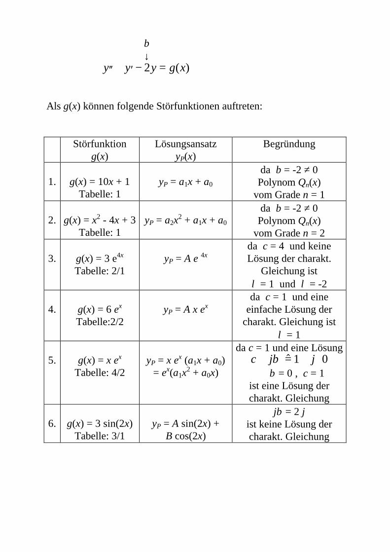
b↓

′′ + ′ − =y y y g x2 ( )

Als g(x) können folgende Störfunktionen auftreten:

Störfunktiong(x)

LösungsansatzyP(x)

Begründung

1. g(x) = 10x + 1Tabelle: 1

yP = a1x + a0

da b = -2 ≠ 0Polynom Qn(x)

vom Grade n = 1

2. g(x) = x2 - 4x + 3Tabelle: 1

yP = a2x2 + a1x + a0

da b = -2 ≠ 0Polynom Qn(x)

vom Grade n = 2

3. g(x) = 3 e4x

Tabelle: 2/1yP = A e 4x

da c = 4 und keineLösung der charakt.

Gleichung istλ = 1 und λ = -2

4. g(x) = 6 ex

Tabelle:2/2yP = A x ex

da c = 1 und eineeinfache Lösung der

charakt. Gleichung istλ = 1

5. g(x) = x ex

Tabelle: 4/2yP = x ex (a1x + a0)

= ex(a1x2 + a0x)

da c = 1 und eine Lösungc j j+ = + ⋅β $ 1 0⇒ β = 0 , c = 1

ist eine Lösung dercharakt. Gleichung

6. g(x) = 3 sin(2x)Tabelle: 3/1

yP = A sin(2x) +B cos(2x)

jβ = 2 jist keine Lösung dercharakt. Gleichung

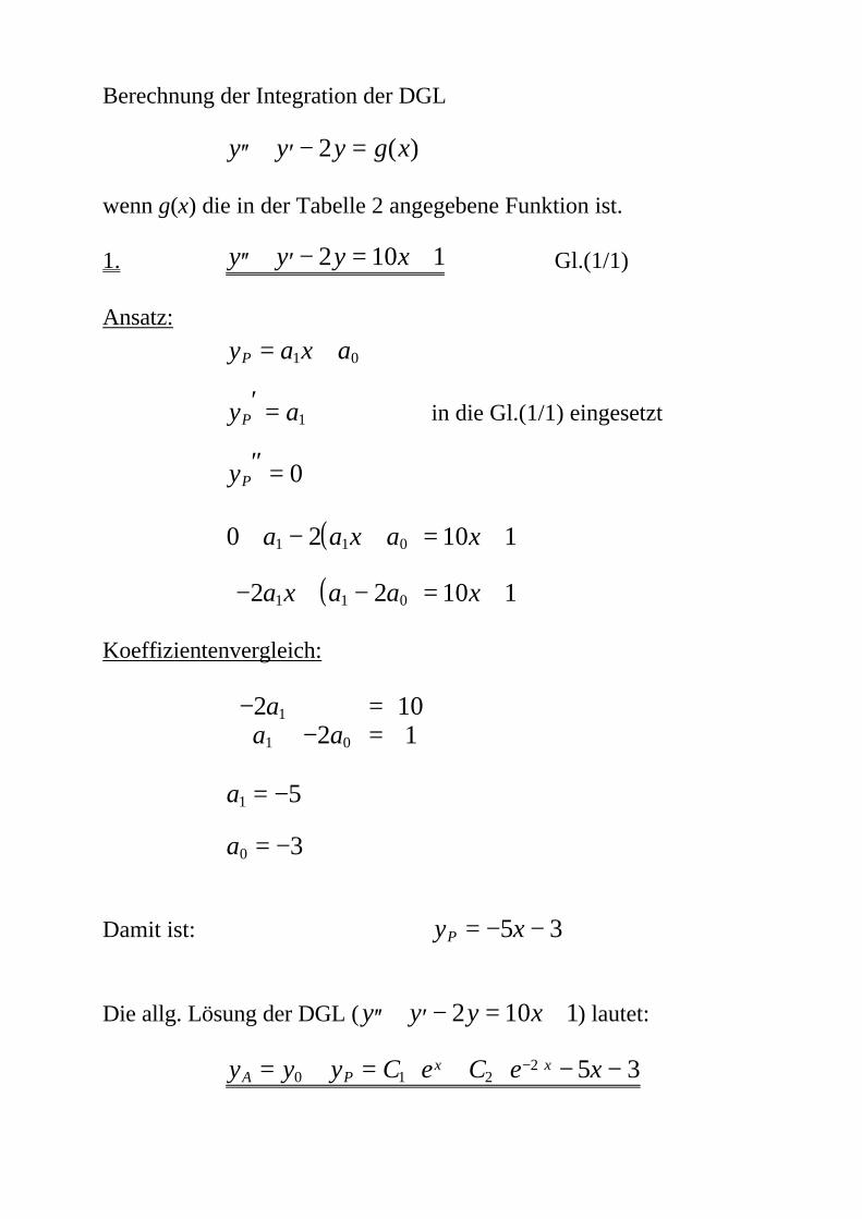
Berechnung der Integration der DGL

′′ + ′ − =y y y g x2 ( )

wenn g(x) die in der Tabelle 2 angegebene Funktion ist.

1. ′′ + ′ − = +y y y x2 10 1 Gl.(1/1)

Ansatz:

y a x a

y a

y

P

P

P

= +

′ =

″ =

1 0

1

0

in die Gl.(1/1) eingesetzt

( )

( )

0 2 10 1

2 2 10 1

1 1 0

1 1 0

+ − + = +

− + − = +

a a x a x

a x a a x

Koeffizientenvergleich:

− =− =

2 10

2 11

1 0

aa a

a

a

1

0

5

3

= −

= −

Damit ist: y xP = − −5 3

Die allg. Lösung der DGL ( ′′ + ′ − = +y y y x2 10 1) lautet:

y y y C e C e xA Px x= + = ⋅ + ⋅ − −− ⋅

0 1 22 5 3

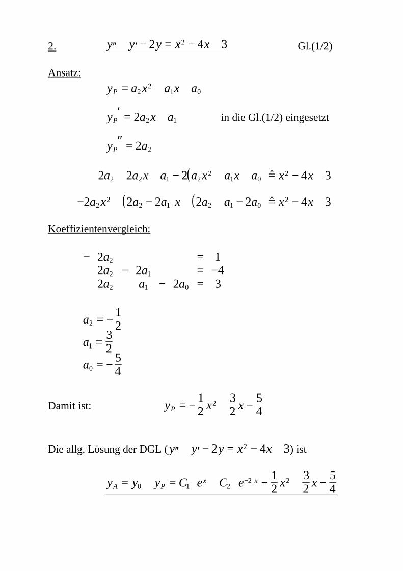
2. ′′ + ′ − = − +y y y x x2 4 32 Gl.(1/2)

Ansatz:

y a x a x a

y a x a

y a

P

P

P

= + +

′ = +

″ =

22

1 0

2 1

2

2

2

in die Gl.(1/2) eingesetzt

( )

( ) ( )

2 2 2 4 3

2 2 2 2 2 4 3

2 2 1 22

1 02

22

2 1 2 1 02

a a x a a x a x a x x

a x a a x a a a x x

+ + − + + = − +

− + − + + − = − +

$

$

Koeffizientenvergleich:

− =− = −+ − =

2 12 2 42 2 3

2

2 1

2 1 0

aa aa a a

a

a

a

2

1

0

12

32

54

= −

=

= −

Damit ist: y x xP = − + −12

32

54

2

Die allg. Lösung der DGL ( ′′ + ′ − = − +y y y x x2 4 32 ) ist

y y y C e C e x xA Px x= + = ⋅ + ⋅ − + −− ⋅

0 1 22 21

232

54

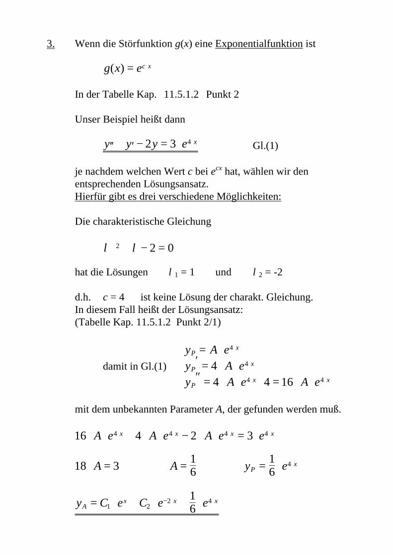
3. Wenn die Störfunktion g(x) eine Exponentialfunktion ist

g x ec x( ) = ⋅

In der Tabelle Kap. 11.5.1.2 Punkt 2

Unser Beispiel heißt dann

′′ + ′ − = ⋅ ⋅y y y e x2 3 4 Gl.(1)

je nachdem welchen Wert c bei ecx hat, wählen wir denentsprechenden Lösungsansatz.Hierfür gibt es drei verschiedene Möglichkeiten:

Die charakteristische Gleichung

λ λ2 2 0+ − =

hat die Lösungen λ1 = 1 und λ2 = -2

d.h. c = 4 ist keine Lösung der charakt. Gleichung.In diesem Fall heißt der Lösungsansatz:(Tabelle Kap. 11.5.1.2 Punkt 2/1)

damit in Gl.(1)

y A ey A ey A e A e

Px

Px

Px x

= ⋅′ = ⋅ ⋅″ = ⋅ ⋅ ⋅ = ⋅ ⋅

⋅

⋅

⋅ ⋅

4

4

4 4

44 4 16

mit dem unbekannten Parameter A, der gefunden werden muß.

16 4 2 34 4 4 4⋅ ⋅ + ⋅ ⋅ − ⋅ ⋅ = ⋅⋅ ⋅ ⋅ ⋅A e A e A e ex x x x

18 3⋅ =A ⇒ A = 16 ⇒ y eP

x= ⋅ ⋅16

4

y C e C e eAx x x= ⋅ + ⋅ + ⋅− ⋅ ⋅

1 22 41

6

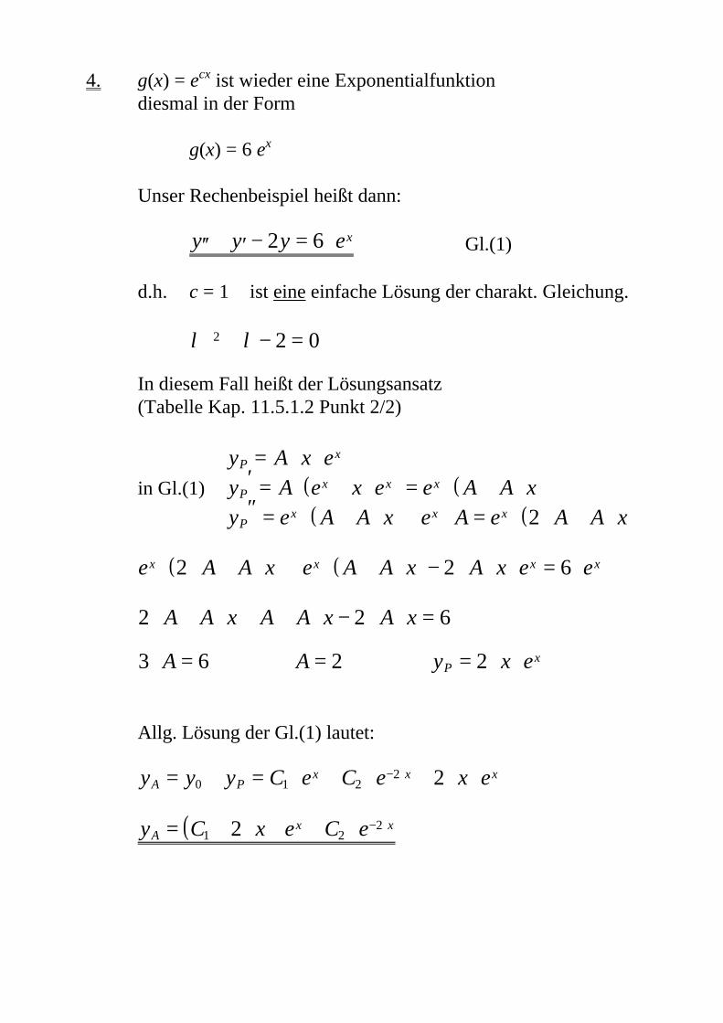
4. g(x) = ecx ist wieder eine Exponentialfunktiondiesmal in der Form

g(x) = 6 ex

Unser Rechenbeispiel heißt dann:

′′ + ′ − = ⋅y y y ex2 6 Gl.(1)

d.h. c = 1 ist eine einfache Lösung der charakt. Gleichung.

λ λ2 2 0+ − =

In diesem Fall heißt der Lösungsansatz(Tabelle Kap. 11.5.1.2 Punkt 2/2)

in Gl.(1) ( ) ( )( ) ( )

y A x ey A e x e e A A xy e A A x e A e A A x

Px

Px x x

Px x x

= ⋅ ⋅′ = ⋅ + ⋅ = ⋅ + ⋅″ = ⋅ + ⋅ + ⋅ = ⋅ ⋅ + ⋅

2

( ) ( )e A A x e A A x A x e ex x x x⋅ ⋅ + ⋅ + ⋅ + ⋅ − ⋅ ⋅ ⋅ = ⋅2 2 6

2 2 6⋅ + ⋅ + + ⋅ − ⋅ ⋅ =A A x A A x A x

3 6⋅ =A ⇒ A = 2 ⇒ y x ePx= ⋅ ⋅2

Allg. Lösung der Gl.(1) lautet:

y y y C e C e x eA Px x x= + = ⋅ + ⋅ + ⋅ ⋅− ⋅

0 1 22 2

( )y C x e C eAx x= + ⋅ ⋅ + ⋅ − ⋅

1 222

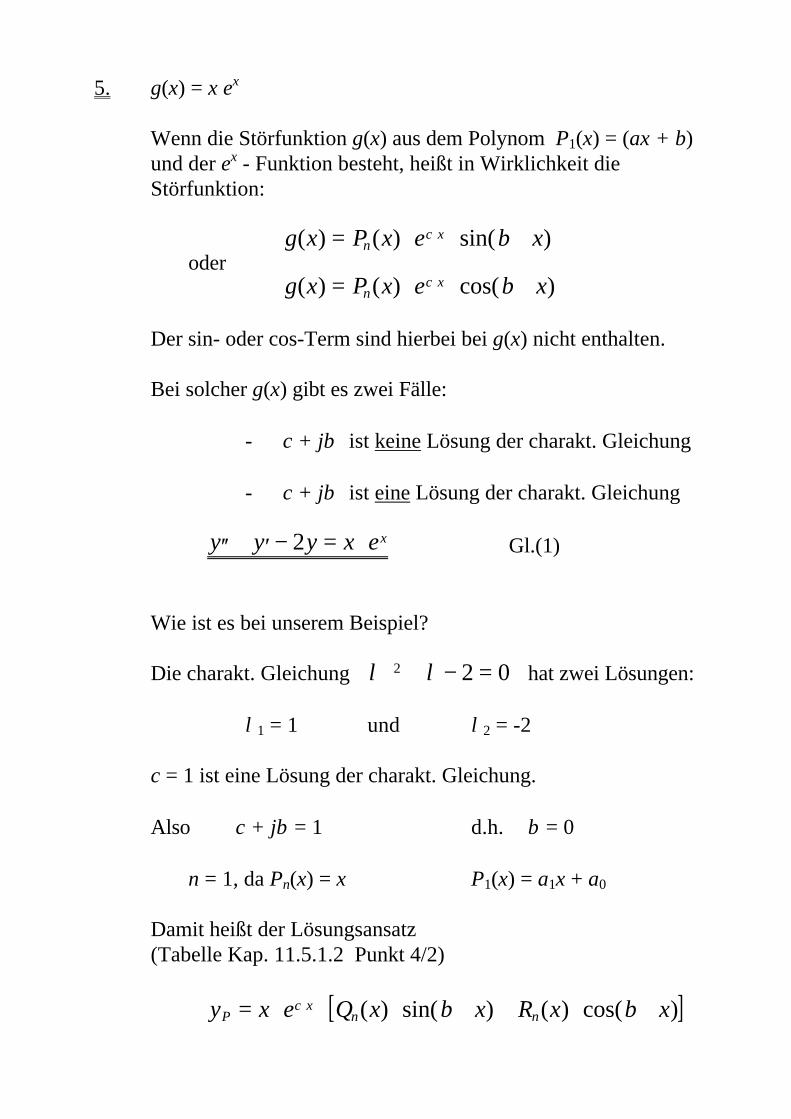
5. g(x) = x ex

Wenn die Störfunktion g(x) aus dem Polynom P1(x) = (ax + b)und der ex - Funktion besteht, heißt in Wirklichkeit die Störfunktion:

oderg x P x e x

g x P x e x

nc x

nc x

( ) ( ) sin( )

( ) ( ) cos( )

= ⋅ ⋅ ⋅

= ⋅ ⋅ ⋅

⋅

⋅

β

β

Der sin- oder cos-Term sind hierbei bei g(x) nicht enthalten.

Bei solcher g(x) gibt es zwei Fälle:

- c + jβ ist keine Lösung der charakt. Gleichung

- c + jβ ist eine Lösung der charakt. Gleichung

′′ + ′ − = ⋅y y y x ex2 Gl.(1)

Wie ist es bei unserem Beispiel?

Die charakt. Gleichung λ λ2 2 0+ − = hat zwei Lösungen:

λ1 = 1 und λ2 = -2

c = 1 ist eine Lösung der charakt. Gleichung.

Also c + jβ = 1 ⇒ d.h. β = 0

n = 1, da Pn(x) = x ⇒ P1(x) = a1x + a0

Damit heißt der Lösungsansatz(Tabelle Kap. 11.5.1.2 Punkt 4/2)

[ ]y x e Q x x R x xPc x

n n= ⋅ ⋅ ⋅ ⋅ + ⋅ ⋅⋅ ( ) sin( ) ( ) cos( )β β

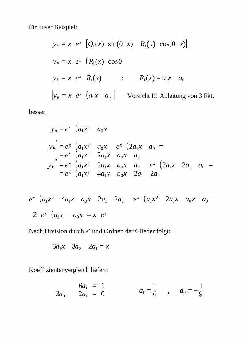
für unser Beispiel:

[ ]y x e Q x x R x xPx= ⋅ ⋅ ⋅ ⋅ + ⋅ ⋅1 10 0( ) sin( ) ( ) cos( )

( )y x e R xPx= ⋅ ⋅ ⋅1 0( ) cos

y x e R xPx= ⋅ ⋅ 1( ) ; R x a x a1 1 0( ) = +

( )y x e a x aPx= ⋅ ⋅ +1 0 Vorsicht !!! Ableitung von 3 Fkt.

besser:

( )

( ) ( )( )( ) ( )( )

y e a x a x

y e a x a x e a x ae a x a x a x a

y e a x a x a x a e a x a ae a x a x a x a a

px

Px x

x

Px x

x

= ⋅ +

′ = ⋅ + + ⋅ + == ⋅ + + +

″ = ⋅ + + + + ⋅ + + == ⋅ + + + +

12

0

12

0 1 0

12

1 0 0

12

1 0 0 1 1 0

12

1 0 1 0

222 2 24 2 2

( ) ( )

( )

e a x a x a x a a e a x a x a x a

e a x a x x e

x x

x x

⋅ + + + + + ⋅ + + + −

− ⋅ ⋅ + = ⋅

12

1 0 1 0 12

1 0 0

12

0

4 2 2 2

2

Nach Division durch ex und Ordnen der Glieder folgt:

6 3 21 0 1a x a a x+ + =

Koeffizientenvergleich liefert:

6 13 2 0

1

0 1

aa a

=+ =

⇒ a116= , a0

19= −

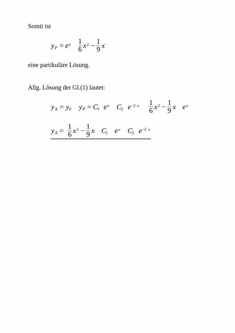
Somit ist

y e x xPx= ⋅ −

16

19

2

eine partikuläre Lösung.

Allg. Lösung der Gl.(1) lautet:

y y y C e C e x x eA Px x x= + = ⋅ + ⋅ + −

⋅− ⋅

0 1 22 21

619

y x x C e C eAx x= − +

⋅ + ⋅ − ⋅1

619

21 2

2

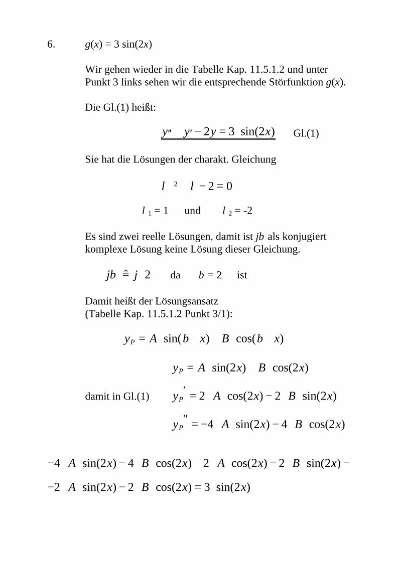
6. g(x) = 3 sin(2x)

Wir gehen wieder in die Tabelle Kap. 11.5.1.2 und unter Punkt 3 links sehen wir die entsprechende Störfunktion g(x).

Die Gl.(1) heißt:

′′ + ′ − = ⋅y y y x2 3 2sin( ) Gl.(1)

Sie hat die Lösungen der charakt. Gleichung

λ λ2 2 0+ − =

λ1 = 1 und λ2 = -2

Es sind zwei reelle Lösungen, damit ist jβ als konjugiert komplexe Lösung keine Lösung dieser Gleichung.

j jβ $= ⋅ 2 da β = 2 ist

Damit heißt der Lösungsansatz(Tabelle Kap. 11.5.1.2 Punkt 3/1):

y A x B xP = ⋅ ⋅ + ⋅ ⋅sin( ) cos( )β β

damit in Gl.(1)

y A x B x

y A x B x

y A x B x

P

P

P

= ⋅ + ⋅

′ = ⋅ ⋅ − ⋅ ⋅

″ = − ⋅ ⋅ − ⋅ ⋅

sin( ) cos( )

cos( ) sin( )

sin( ) cos( )

2 2

2 2 2 2

4 2 4 2

− ⋅ ⋅ − ⋅ ⋅ + ⋅ ⋅ − ⋅ ⋅ −

− ⋅ ⋅ − ⋅ ⋅ = ⋅

4 2 4 2 2 2 2 2

2 2 2 2 3 2

A x B x A x B x

A x B x x

sin( ) cos( ) cos( ) sin( )

sin( ) cos( ) sin( )

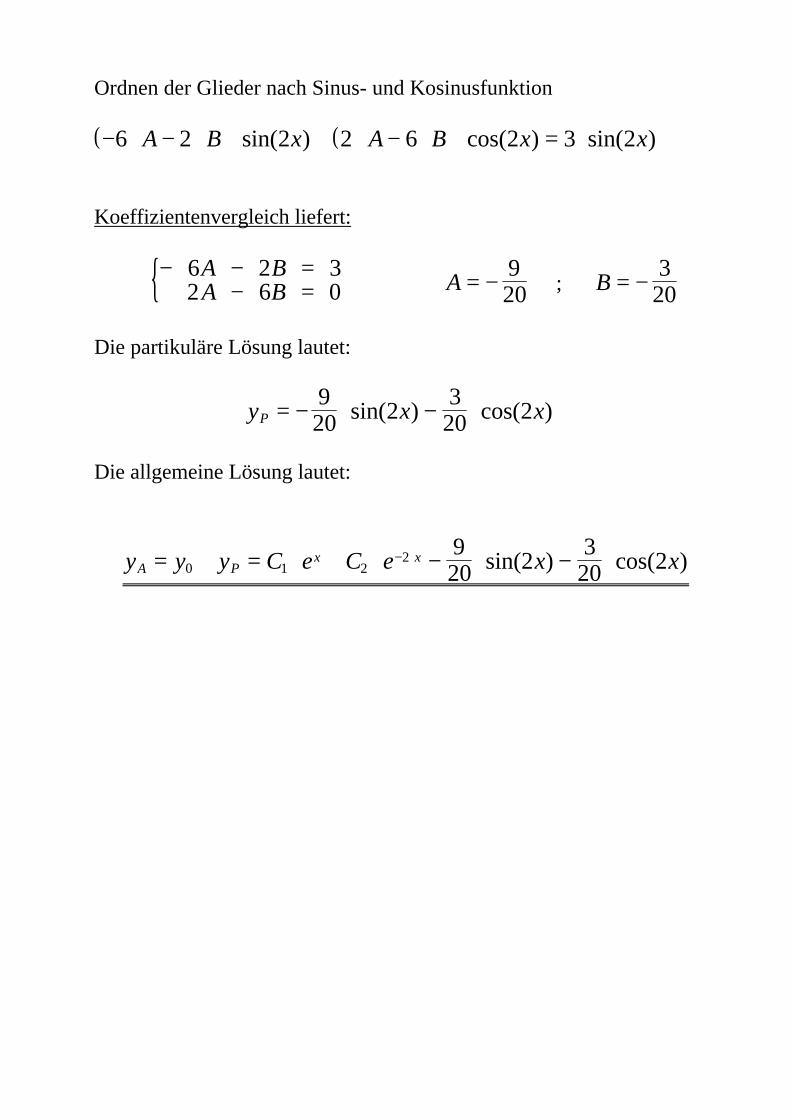
Ordnen der Glieder nach Sinus- und Kosinusfunktion

( ) ( )− ⋅ − ⋅ ⋅ + ⋅ − ⋅ ⋅ = ⋅6 2 2 2 6 2 3 2A B x A B x xsin( ) cos( ) sin( )

Koeffizientenvergleich liefert:

{− − =− =

6 2 32 6 0

A BA B ⇒ A = − 9

20 ; B = − 320

Die partikuläre Lösung lautet:

y x xP = − ⋅ − ⋅920 2

320 2sin( ) cos( )

Die allgemeine Lösung lautet:

y y y C e C e x xA Px x= + = ⋅ + ⋅ − ⋅ − ⋅− ⋅

0 1 22 9

20 23

20 2sin( ) cos( )