Embed Size (px)
Citation preview

Friedrich-Alexander-Universität Erlangen-Nürnberg
Institute for Electronics Engineering
Prof. Dr.-Ing. Dr.-Ing. habil. Robert Weigel
Prof. Dr.-Ing. Georg Fischer
Master Thesis
Course of Study
Industrial Engineering
by
Carlos Martínez Cantón
on the Subject
Optimization of the transmitter setup for a molecular
communication link based on superparamagnetic iron
nanoparticles
Supervisors: Prof. Dr.-Ing. Georg Fischer
Dr. rer. nat. Jens Kirchner
Begin: 15.04.2018
Submission: 15.10.2018


Optimization of the transmitter setup for a molecular communication
link based on superparamagnetic iron nanoparticles


Erklärung
A
Ich versichere, dass ich die Arbeit ohne fremde Hilfe und ohne Benutzung anderer als der
gegebenen Quellen angefertigt habe und dass die Arbeit in gleicher oder ähnlicher Form
noch keiner anderen Prüfungsbehörde vorgelegen hat und von dieser als Teil einer
Prüfungsleistung angenommen wurde.
Alle Ausführungen, die wörtlich oder sinngemäβ übernommen wurden, sind als solche
gekennzeichnet.
Erlangen, den 15. Oktober 2018
Carlos Martínez Cantón


Kurzfassung
A
Die Suche nach innovativen Anwendungen in den Bereichen Biomedizin und
Nanotechnologie kommt dem weiteren Fortschritt in der molekularen
Kommunikationsforschung zugute. Dennoch ist ein voll funktionsfähiges künstliches
molekulares System noch keine Realität. Das Institut für Elektronik der FAU hat ein
experimentelles molekularkommunikatives Testbed auf Basis magnetischer Nanopartikel
entwickelt, das sich als effektiv bei der Übertragung von Bitsequenzen erwiesen hat, die
von SPIONs kodiert werden. Im Rahmen dieser Arbeit wurde eine Optimierung des
Senders dieses Setups implementiert und getestet. Diese Optimierung basiert auf der
Lenkung von SPIONs über einen gewünschten Weg nach einer Aufspaltung unter
Verwendung der magnetischen Kraft, die von einem Elektromagneten erzeugt wird, der
sich taktisch in der Nähe der Röhren befindet, in denen die Nanopartikel fließen. Die
Größe des Elektromagneten wurde im Verhältnis zu der Röhrengröße des Systems
ausgewählt. Außerdem wurde eine elektronische Steuerschaltung zum automatschen
Schalten des Elektromagneten entworfen und auf einem Protoboard montiert. Die
Messung der Mengen an magnetischen Partikeln in den Röhren des Systems erfolgt unter
Verwendung einer Suszeptometerspule, einer elektronischen Vorrichtung, durch die sich
die magnetischen Partikel bewegen und ein elektronisches Signal erzeugen.
Es werden experimentelle Ergebnisse für magnetische Suszeptibilitätsänderungen in
beiden Kanälen nach dem Y-Verbinder vorgestellt. Sie fielen nicht wie erwartet aus,
weshalb Empfehlungen gegeben werden, um zuverlässige Messungen zu erhalten und die
vorgestellte Forschungsarbeit weiter voranzutreiben.


Abstract
The search for innovative applications in the fields of biomedicine and nanotechnology
benefit the further advance in molecular communication research. Nevertheless, a fully-
functional artificial molecular system is not yet a reality. Institute for Electronics
Engineering from FAU has developed an experimental molecular communication testbed
based on magnetic nanoparticles, which has demonstrated to be effective in the
transmission of bit sequences encoded by SPIONs. As part of this work, an optimization
of the transmitter of this setup is implemented and tested. This optimization is based on
the steering of SPIONs through a desired path after a splitting by use of the magnetic
force generated by an electromagnet, which is located tactically in the proximity of the
tubes where the nanoparticles flow. The electromagnet size has been selected in
proportion to the tubes size of the system. Also, an electronic control circuit to switch
automatically the electromagnet has been designed and mounted on a protoboard.
Measuring of magnetic particles amount in the tubes of the system is accomplished using
a susceptometer coil, an electronic device where the magnetic particles move through and
generate an electrical signal.
Experimental results for magnetic susceptibility changes in both channels after the Y-
connector are presented. They have not been as expected, thus, recommendations in order
to acquire more reliable measurements and further advancing in the presented research
work are given.


A
Abbreviations
A
FAU Friedrich-Alexander-Universität Erlangen-Nürnberg
SPION Superparamagnetic Iron Oxide Nanoparticle
MC Molecular Communication
TX Transmitter
RX Receiver
pH Potential of Hydrogen
MRI Magnetic Resonance Imaging
GUI Graphical User Interface
DC Direct Current
BJT Bipolar Junction Transistor
LED Light Emitting Diode
PIC Programmable Intelligent Computer

Contents
Abbreviations xi
1 Introduction 1
2 Fundamentals 3
2.1 Molecular Communication ..................................................................................... 3
2.2 Magnetism .............................................................................................................. 6
2.2.1 Paramagnetism.............................................................................................. 7
2.2.2 Superparamagnetism .................................................................................... 9
2.2.3 Superparamagnetic Iron Oxide Nanoparticles .............................................. 9
2.3 Solenoids and Electromagnets .............................................................................. 11
2.3.1 Magnetic Force Generated by an Electromagnet on a SPION ................... 12
3 Current Molecular Communication System 15
4 Optimization of the Current System 19
4.1 Testbed to Steer the SPIONs ................................................................................ 19
4.1.1 Electromagnet ............................................................................................. 20
4.1.2 Control Circuit to Switch the Electromagnet ............................................. 22
4.1.2.1 Microcontroller .............................................................................. 24
4.1.2.2 Transistor ....................................................................................... 26
4.1.2.3 Rectifier Diode .............................................................................. 26
4.1.2.4 LED and Resistor........................................................................... 27
4.1.2.5 Potentiometer ................................................................................. 27
4.1.3 Simulation of the Control Circuit ............................................................... 29
4.1.4 Testing of the Control Circuit ..................................................................... 30
5 Results and Discussion 33
5.1 Testing without Susceptometer ............................................................................ 33

5.2 Testing using a Susceptometer ............................................................................. 39
5.2.1 Results of Testing using a Susceptometer .................................................. 43
5.2.2 Problems during Testing ............................................................................. 49
6 Conclusion and Outlook 51
6.1 Conclusion ............................................................................................................ 51
6.2 Outlook ................................................................................................................. 53
A Appendix 55
List of Figures 57
List of Tables 59
Bibliography 61

Chapter 1
Introduction
A
The interest in molecular communication is growing due to the need of transmitting
information at micro- or nanoscale. Communication using small particles in areas
impenetrable for electromagnetic waves is an alternative for many applications in the field
of biomedicine or nanotechnology, such as drug targeting or monitoring of chemical
reactors [1]. Nevertheless, a fully-functional artificial communication system has not
been realized yet.
Institute for Electronics Engineering from Friedrich-Alexander-Universität Erlangen-
Nürnberg (FAU) has developed an artificial molecular communication system in the size
range of several cm [2], but now realizing it at nanoscale remains a challenge. The testbed
emulates blood vessels by use of tubes, where superparamagnetic iron oxide nanoparticles
(SPIONs) are transported and used as information carriers. These particles are a type of
artificial particles well-established in biotechnology and biocompatible [3]; they are also
clinically safe and do not interfere with other chemical processes like acids and bases
would do, which makes them attractive for applications such as the monitoring of
chemical reactors where particles stored in a reservoir could be released upon an event
like the detection of a defect. Moreover, they can be attracted by an external magnetic
field generated by a magnet or a solenoid and externally visualized, which can help
detection and supervision.
The mentioned setup above is based on the injection and transportation of these magnetic
nanoparticles along a propagation tube using two electronic pumps. The particles are
transported a certain distance until being detected by an electric coil, whose current is
affected by the magnetic nanoparticles moving through its core. The signal detected by
the coil is used to determine the transmitted binary sequence. When particles move

2 Chapter 1 Introduction
through the coil, binary “1”is detected; if particles are absent, this is interpreted as binary
“0”.
The system works properly and it is capable of transmitting encoded messages as binary
bits. Now, the goal is to optimize the transmission setup trying to guide the particles
through a specific path. In this work, one alternative is proposed, which consists in
steering the magnetic nanoparticles with a controlled external magnetic field generated
by an electromagnet. It is located tactically in the proximity of the propagation tube so
that the nanoparticles flow towards the desired direction after a Y-connector.
In the following chapter, basics of molecular communication, magnetism, SPIONs and
electromagnets are given. Chapter 3 summarizes briefly the current testbed developed by
Institute for Electronics Engineering from FAU. Chapter 4 presents the new setup it has
been tested together with the electronic circuit designed to control automatically the
switch of the electromagnet. In Chapter 5 the results acquired from several experiments
with the new testbed are presented. The present work concludes by a summary of results
and an outlook for future improvements is suggested.
Chapter 2
Fundamentals
A
This chapter presents some fundamentals of molecular communication, magnetism,
magnetic nanoparticles that are used in molecular communication systems,
electromagnets and its magnetic theory. These fundamentals shall help to understand the
basic molecular communication notions and the basic physics and electromagnetism
concepts in the field of electromagnets.
2.1 Molecular Communication
Modern communication systems work with electrical or electromagnetic signals.
However, there are applications in which this is inefficient or inappropriate, like for
instance, at sizes extremely small. This is the case of communication among devices at
micro- or nanoscale (e.g., nanorobots), due to restrictions regarding the antenna size and
the wavelength of the electromagnetic signal [4]. Because of these limitations, appears
the necessity to search for innovative communication systems that use other sort of
propagation signal.
At the same time, progresses in nanotechnology, which make possible to miniaturize a
lot of devices, and the development in biotechnology, boost the scale reduction of
information systems. From here emerges the idea of molecular systems at sizes of micro-
or nanometers that are inspired by nature. Molecular communication (MC) bases on a
biological form of communication, where chemical signals are used to transfer
information, likewise many living beings do it through molecules.

4 Chapter 2 Fundamentals
As illustrated in Figure 2.1, a MC system is composed of three main components, like
conventional communication systems: a transmitter (TX), a receiver (RX) and a channel.
In MC, the information is contained in particles whose size is micrometric or nanometric.
These particles can be biological (like hormones, proteins, pheromones, etc.) or synthetic
(like SPIONs). The TX provides the energy required to generate and propagate the
particles through the channel, which tend to be an aqueous one (like blood in living
organisms) or a gaseous one (like air). When a particle acting as information carrier
arrives at the RX, then it is detected and decoded in order to interpret the information
included in the particle.
Figure 2.1: Schematic representation of molecular communication between a
transmitter (TX) and a receiver (RX). Particles released by the TX are the
information carriers and are represented as red circles [5].
The main advantages of MC compared to conventional communication systems are: the
first one is that MC signals can be biocompatible, like SPIONs used for drug targeting
applications (there are others that are not, like acids and bases, which interfere with other
chemical processes) and, thus, with possibility to be used in living organisms. The second
one is the greater energy efficiency of MC systems. Furthermore, it is suitable for use in
nanomachines. Regarding its general disadvantages, molecules propagation presents
randomness, which implies noise in the propagation signal. Also, the propagation time is
rather long and the biological particles can be affected by their environment (temperature,
pH, among others). Even so, MC signals are ideal for many applications where use of
electromagnetic signals is not appropriate or not desirable.

2.1 Molecular Communication 5
There is a large number of possible applications for MC in different fields, some of which
are:
Health sector: targeted drug delivery, reconstruction of tissues and damaged
organs, modification of the sequences of human genes, localization and reaction
with malicious cells (i.e., cancer).
Environment: environmental monitoring to detect polluting and toxins, control
the quality of water and food.
Manufacturing: develop new materials and manufacturing processes, quality
control by identification of defects in products.
Others: interact with insects, animals or plants, monitoring of infrastructures,
robotic communication.
Although MC systems offer a new option of communication and have a high applicability
in several fields, they still present limits. Thus, more experimentation is required in order
to further advance molecular communication research.
In next section, basics of magnetism and an explanation of a type of synthetic magnetic
particles used in molecular communication systems (SPIONs) are given.

6 Chapter 2 Fundamentals
2.2 Magnetism
Magnetism is the phenomenon by which materials attract or repel other materials from a
distance. All substances have magnetic properties. It is well-known the magnetic
properties of iron, which is used in compasses or components from electric systems. But,
other materials different from iron have also magnetic properties, although to a lesser
extent.
Magnetic fields are generated by the movement of an individual electric charge or a
combination of electric charges (electrical current); they can also be produced by some
materials like permanent magnets. When a charged particle spin (like electrons spin at
atomic scale), it generates a magnetic dipole. Applying an external magnetic field on the
material, their magnetic dipoles align to the field causing a magnetic moment in the
material.
When an external magnetic field (units A/m) reaches a material, the magnetic field
(units Tesla) induced in it is [6]:
= µ0( + ) (2.1)
where µ0 is the permeability of vacuum (1.257×10⁻⁶ H/m) and (units A/m) is the
magnetization of the substance, which is produced due to the alignment of the magnetic
dipoles of the substance with the external field.
The magnetic susceptibility 𝜒 (dimensionless in SI units) is a magnitude that relates this
magnetization and the external magnetic field [6]:
= 𝜒 (2.2)
It is a characteristic magnitude of materials that indicates how sensitive the material is to
a magnetic field. The greater it is, the more magnetizable the material is.
According to the response of a material in the presence of an external non-uniform
magnetic field, it is classified as diamagnetic, paramagnetic or ferromagnetic. Some
examples of diamagnetic materials are water, copper or lead; some of paramagnetic ones
are aluminium or magnesium; some of ferromagnetic ones are iron, nickel or cobalt.

2.2 Magnetism 7
Diamagnetic substances (𝜒 < 0) are repelled from regions with high magnetic field,
whereas paramagnetic ones (𝜒 > 0) are attracted to them. On the other hand,
ferromagnetic materials (𝜒 > 0) present magnetic properties, even when the applied
magnetic field is removed. The attraction of ferromagnetic substances towards high
magnetic areas is stronger than that of paramagnets.
In this work, SPIONs are used as information carriers in the molecular communication
testbed. In order to understand better their behaviour under the influence of an external
magnetic field, some fundamentals of paramagnetism and superparamagnetism are
presented in the following.
2.2.1 Paramagnetism
Paramagnetic materials are those that in the presence of a magnetic field gradient, move
towards the area with higher magnetic field intensity. These substances experience the
same type of attraction and repulsion like magnets. However, they are not permanently
magnetized, since when the applied magnetic field disappears, also the induced magnetic
alignment of their magnetic dipoles does (see Figure 2.2) and, thus, causing its
demagnetization.
Figure 2.2: Schematic representation of magnetic dipoles of a paramagnetic material
under the influence of an applied magnetic field gradient. The magnetic
dipoles are randomly oriented in the absence of a magnetic field (the net
magnetic moment of the material is zero). When a magnetic field gradient
is applied, the magnetic dipoles align themselves in the same direction of
the field [7].
The magnetic permeability of a substance (µ) is its capacity to attract or being passed
through by a magnetic field; the relative magnetic permeability (µ𝑟) is its magnetic
permeability compared to vacuum magnetic permeability (µ0):

8 Chapter 2 Fundamentals
µ𝑟 = µ
µ0 (2.3)
Paramagnetic materials are slightly more magnetically permeable than the vacuum (µ ≥
1) and have a very small and positive magnetic susceptibility (𝜒 > 0). For that reason,
they are weakly attracted by magnetic fields and as previously mentioned, they do not
keep their properties as soon as the magnetic field disappears.
This weak attraction force is due to the fact that the magnetic dipoles of the material are
completely disordered (see Figure 2.2) in such natural state, causing that the magnetic
field was only able to orient them lightly.
The magnetization of a paramagnet is determined by Curie’s law:
𝑀 = 𝐶 ·
𝐵
𝑇 (2.4)
where T is the absolute temperature in Kelvin and C a constant that depend on the
material. From this law, we can observe that paramagnetic materials tend to be more
magnetic as higher is the applied magnetic field, and less magnetic as higher is the
temperature. Nevertheless, when the paramagnetic material is near its magnetic saturation
Ms (moment in which most of its magnetic dipoles are aligned to the field), then this law
is not applicable, since as Figure 2.3 shows, the relation magnetization-magnetic field is
not linear.
Figure 2.3: Magnetization curves for ferromagnetic, paramagnetic and
superparamagnetic materials. Ms: magnetic saturation; MR: remnant
magnetization [8].
Among paramagnetic materials exists special ones called superparamagnetics. In next
section, a brief description of them is presented.

2.2 Magnetism 9
2.2.2 Superparamagnetism
Superparamagnetism is a phenomenon presented in some materials, which show
paramagnetic properties under specific critic temperatures. It occurs at small scale, like
in nanoparticles of approximately 20 nm or less, when the energy required to change the
direction of the particles is similar to the ambient thermal energy. It causes that a
significant number of particles of the material change direction randomly over short
periods. In such state, they act as paramagnetic particles, allowing its magnetization under
the influence of an applied magnetic field. However, they present a greater magnetic
susceptibility than paramagnetic particles.
Superparamagnetic particles have a remnant magnetisation MR (persistent magnetization
on the material when the applied magnetic field is removed) of zero, which implies they
can be demagnetized rapidly, even when they are saturated (M = Ms). They are
magnetized in the presence of a magnetic field, but they are demagnetized as soon as the
field disappears. Consequently, their M-H curve shows no hysteresis (see Figure 2.3); this
property is important for reducing the tendency of the particles to agglomerate [9].
These kind of substances are used for magnetic resonance imaging (MRI), for drug
delivery, for cell separation and cell labelling applications, among others [10].
In the following, a type of superparamagnetic particles that are used in molecular
communication systems is described.
2.2.3 Superparamagnetic Iron Oxide Nanoparticles
Superparamagnetic iron oxide nanoparticles (SPIONs) are a kind of particles with sizes
around few tens of nm which are used in many research studies regarding biotechnology
and biomedicine. Their widespread use is due to the large number of possible applications
where they can be used, especially on health sector, as well as their low cost, strong
adsorption capacity, easy separation and enhanced stability [11].
SPIONs are composed of maghemite, magnetite or hermatite [12] and they can be
synthetized by physical, chemical or biological methods (e.g., co-precipitation, high
temperature decomposition, etc.) [13].
They present superparamagnetic properties, thus, in a natural state their total net magnetic
moment is zero (the magnetic dipoles of the nanoparticle are randomly oriented), but
under the influence of an external magnetic field they are magnetized; they become again
10 Chapter 2 Fundamentals
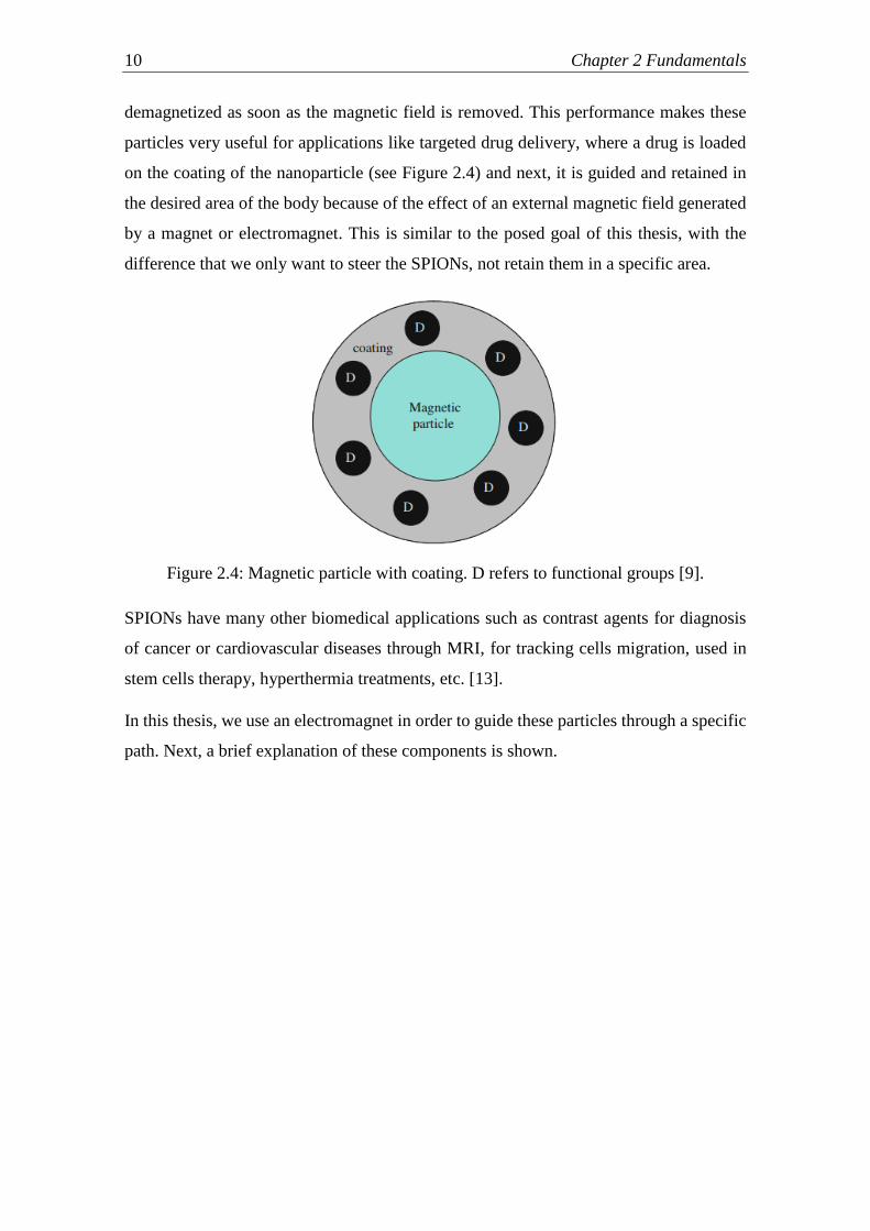
demagnetized as soon as the magnetic field is removed. This performance makes these
particles very useful for applications like targeted drug delivery, where a drug is loaded
on the coating of the nanoparticle (see Figure 2.4) and next, it is guided and retained in
the desired area of the body because of the effect of an external magnetic field generated
by a magnet or electromagnet. This is similar to the posed goal of this thesis, with the
difference that we only want to steer the SPIONs, not retain them in a specific area.
Figure 2.4: Magnetic particle with coating. D refers to functional groups [9].
SPIONs have many other biomedical applications such as contrast agents for diagnosis
of cancer or cardiovascular diseases through MRI, for tracking cells migration, used in
stem cells therapy, hyperthermia treatments, etc. [13].
In this thesis, we use an electromagnet in order to guide these particles through a specific
path. Next, a brief explanation of these components is shown.
2.3 Solenoids and Electromagnets 11
2.3 Solenoids and Electromagnets
In order to guide SPIONs through a desired way, an electromagnet is used. This
component steers the nanoparticles under the influence of a magnetic field or more
precisely, under the influence of a magnetic field gradient.
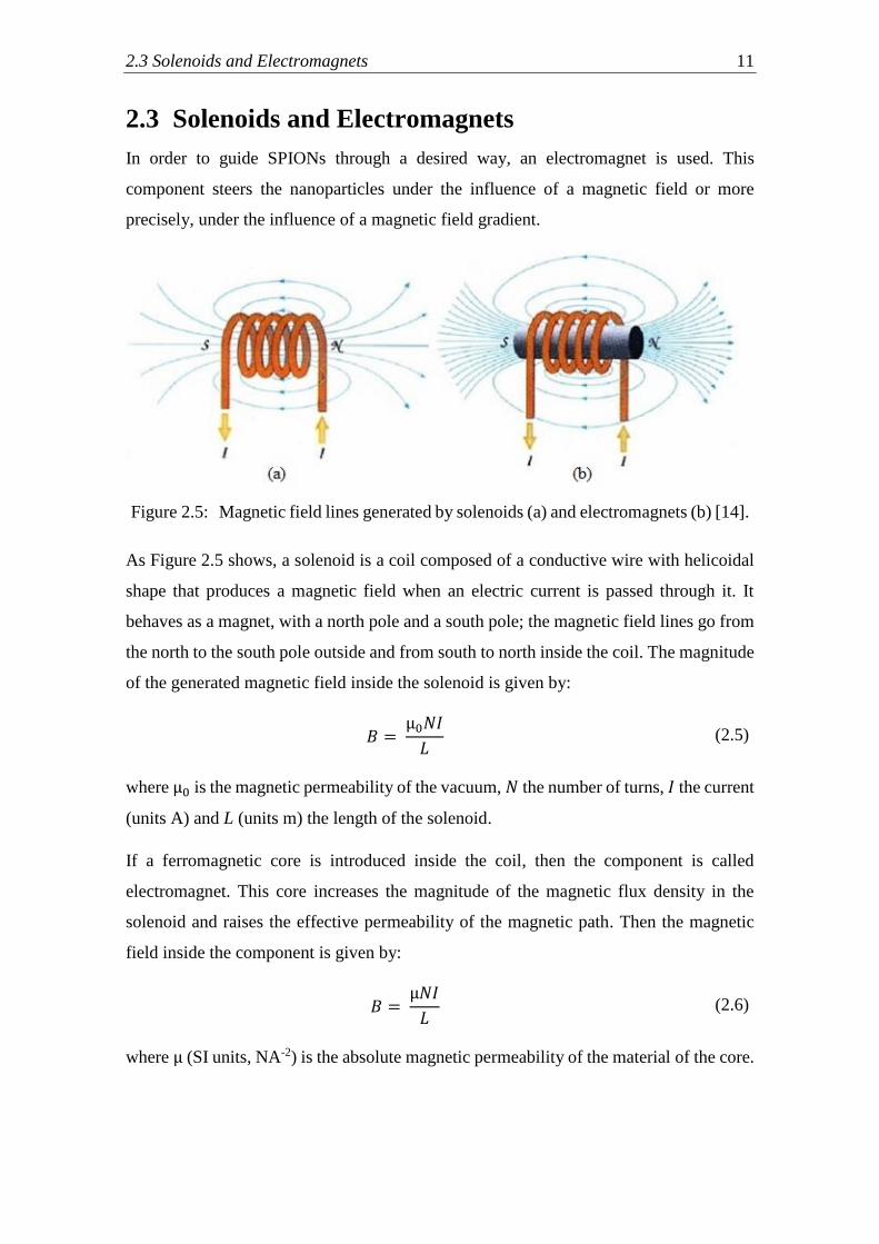
Figure 2.5: Magnetic field lines generated by solenoids (a) and electromagnets (b) [14].
As Figure 2.5 shows, a solenoid is a coil composed of a conductive wire with helicoidal
shape that produces a magnetic field when an electric current is passed through it. It
behaves as a magnet, with a north pole and a south pole; the magnetic field lines go from
the north to the south pole outside and from south to north inside the coil. The magnitude
of the generated magnetic field inside the solenoid is given by:
𝐵 = µ0𝑁𝐼
𝐿 (2.5)
where µ0 is the magnetic permeability of the vacuum, 𝑁 the number of turns, 𝐼 the current
(units A) and L (units m) the length of the solenoid.
If a ferromagnetic core is introduced inside the coil, then the component is called
electromagnet. This core increases the magnitude of the magnetic flux density in the
solenoid and raises the effective permeability of the magnetic path. Then the magnetic
field inside the component is given by:
𝐵 = µ𝑁𝐼
𝐿 (2.6)
where µ (SI units, NA-2) is the absolute magnetic permeability of the material of the core.

12 Chapter 2 Fundamentals
2.3.1 Magnetic Force Generated by an Electromagnet on a
SPION
Since in this work and many other applications in biomedicine require to manipulate the
path of the nanoparticles, it is appropriate to understand the force required to do so. Some
research studies about this topic, where several magnets or magnetic elements of different
geometries are taking into account, have been accomplished; see for example references
[15], [16]. But not for the specific case of an electromagnet.
As indicated in reference [6], the general equation for the magnetic force generated by a
non-homogenous magnetic field on a nanoparticle in solution is:
𝐹 𝑚 = 𝜒𝑝−𝜒𝑠
µ0𝑉( · ) (2.7)
being 𝜒𝑝 and 𝜒𝑠 the magnetic susceptibilities of the particle and the solvent, respectively.
In this work we use SPIONs dispersed in an aqueous suspension. In particular, lauric acid
coated SPIONs (SPIONLA) with a hydrodynamic particle radius of 27.5 nm are used, thus,
𝜒𝑝 is the magnetic susceptibility of a SPION (7.28×10⁻³ in SI units) and 𝜒𝑠 is the magnetic
susceptibility of the water (-9.04×10⁻⁶ in SI units) .
Consider now the case of this work, where the magnetic force generated by an
electromagnet is used to divert the trajectory of SPIONs flowing in the system in order to
steer them through the correct path after a splitting, as illustrated in Figure 2.6.

2.3 Solenoids and Electromagnets 13
Figure 2.6: Schematic of the steering of a SPION through a specific path (described as
correct path) by the influence of the magnetic field generated by an
electromagnet. In red colour the expected SPION trajectory.
Assuming that a SPION is spherical with a radius R, its volume is 𝑉 = 4𝜋𝑅3
3. Therefore,
equation (2.7) transforms into:
𝐹 𝑚 = (𝜒𝑝 − 𝜒𝑤)
µ0·4𝜋𝑅3
3·
(
𝐵𝑥𝜕𝐵𝑥𝜕𝑥
+ 𝐵𝑦𝜕𝐵𝑥𝜕𝑦
+ 𝐵𝑧𝜕𝐵𝑥𝜕𝑧
𝐵𝑥𝜕𝐵𝑦
𝜕𝑥+ 𝐵𝑦
𝜕𝐵𝑦
𝜕𝑦+ 𝐵𝑧
𝜕𝐵𝑦
𝜕𝑧
𝐵𝑥𝜕𝐵𝑧𝜕𝑥
+ 𝐵𝑦𝜕𝐵𝑧𝜕𝑦
+ 𝐵𝑧𝜕𝐵𝑧𝜕𝑧 )
(2.8)
where 𝜒𝑝 is the magnetic susceptibility of the SPION and 𝜒𝑤 the magnetic susceptibility
of the water. To find the magnetic force, thus, it is required to know the components of
the magnetic field vector as well as the various partial derivatives of the magnetic field.
The lack of information regarding the magnetic field generated in external points from an
electromagnet, complicate the resolution of equation (2.8). For the present work, it has
not been considered essential to find a specific solution, rather the current work consists
in studying the possibility to guide the magnetic nanoparticles under the influence of a
magnetic field, regardless of the value it has.


Chapter 3
Current Molecular Communication System
A
In this chapter a brief description of the operation of the current artificial molecular
system developed by Institute for Electronics Engineering from FAU is presented. The
testbed has been demonstrated to be effective sending information encoded as bits
through SPIONs. Now, the main purpose of this work is to optimize the transmitter setup
of this system, thus, a proper understanding of its working is required.
The system developed by FAU (see Figure 3.1) consists in a molecular communication
system based on information transmission through encoded messages by SPIONs.
Specifically, the testbed uses lauric acid coated SPIONs (SPIONLA) as information
carriers because of their magnetic properties. To see detailed parameters of these
nanoparticles, the diameter and length of the tubes, flow rates of the pumps, etc., see
Table I from reference [2].
Figure 3.1: Photograph of the molecular communication system developed by FAU [2].
The particles are stored in a syringe together with water. This syringe is connected via a
tube with an electronic pump (Ismatec® Reglo Digital, Germany), which controls the

16 Chapter 3 Current Molecular Communication System
injection of the mixture through another tube with a constant flow rate and injecting a
dosage volume of few microliters of particle suspension. This tube concludes in a Y-
connector, where a second tube is connected (see Figure 3.2). A second pump (Ismatec®
IPC, Germany) provides a constant background flow of water through this last tube for
signal propagation. At the exit of the Y-connector, it is placed the propagation channel,
through which the sum of particle suspension and background flow is transmitted.
Figure 3.2: Photograph of the Y-connector. The particle tube and the background flow
tube are placed in the entrance of the splitting, whereas the propagation tube
in its exit [2].
For signal reception, it is employed a susceptometer (MS2G Bartington®) at the end of
the propagation channel, an electronic device including a coil, where the magnetic
particles move through and generate an electrical signal 𝜒(t) proportional to the quantity
of magnetic particles flowing in that area; it measures susceptibility changes. This
changes are monitored and recorded with the software Bartsoft (Bartington Instruments,
Witney, UK). Finally, the mixture of SPIONs and water is collected in a waste container.
The system is able to send text messages as encoded bits by SPIONs according to the next
procedure: using a custom LabVIEW (National Instruments, Austin, Texas, USA)
graphical user interface (GUI), the first pump mentioned in this chapter switches the
injection of SPIONs into the propagation channel. When a dose of particle solution arrives
at the susceptometer, then the susceptibility change is interpreted as a bit ”1”; when no
particles are registered in the receiver, then it is interpreted as a bit ”0”. The
synchronization is accomplished using the 8 bit extended ASCII encoding for capital
letters, which is composed of 26 capital letters with a [0, 1, 0] prefix: when the
susceptometer detects the first peak, which belongs to the bit ”1” of the prefix, then the
start of a character is recognised.

Current Molecular Communication System 17
The goal of this work is to optimize the transmitter of this setup using an electromagnet
near the area of the Y-connector in order to steer the SPIONs to a desired path after the
splitting. In next section, the method accomplished for this purpose is described.


Chapter 4
Optimization of the Current System
A
Now that we know how the current system developed by FAU works, a modification of
it is proposed in order to optimize the transmitter. The aim is to steer the SPIONs through
a desired tube under the influence of a magnetic field. For that purpose, an electromagnet
is used. In the following, a detailed description of the circuit used to control the switch of
the electromagnet is presented, as well as the whole testbed used during the experiments.
4.1 Testbed to Steer the SPIONs
A schematic of the testbed proposed to study the efficacy of the magnetic field generated
by the electromagnet on SPIONs is shown in Figure 4.1.
Figure 4.1: Schematic representation of the testbed proposed to check the efficacy of a
magnetic field on SPIONs.

20 Chapter 4 Optimization of the Current System
The mixture of water and SPIONs is pumped by a peristaltic pump towards the Y-
connector with a constant flow. Near the split an electromagnet is placed, so that its
magnetic field steers the magnetic particles through the propagation channel, where the
susceptometer works as receiver of the system. The aim is to attract the maximum
SPIONs towards the susceptometer in order to get a good signal reception. Finally, the
mixture is collected in a waste container.
Next, the chosen electromagnet and the electronic circuit that controls its switch is
presented.
4.1.1 Electromagnet
An electromagnet ITS-MS-2015 from the manufacturer Red Magnets has been selected,
due to its small size and voltage supply rate (see Table 4.1). Including its external case, it
has a diameter of 20 mm and a length of 15 mm, which makes it appropriate to use with
the testbed. We try to use an electromagnet whose size do not exceed very much the size
of the tubes used in the testbed, since it will be placed near them.
Table 4.1: ITS-MS-2015 electromagnet parameters. Information provided in the
datasheet of the component and by the manufacturer.
Parameter Numerical Value
Length 15 mm
Diameter 20 mm
Number of turns N 1000
Series resistance RDC 66 Ω
Inductance 57 mH
Maximum voltage supply 12 V
Maximum power dissipation 2 W
Maximum force 20 N
The electromagnet contains a core composed of 12L12 carbon steel and has a number of
turns of 1000. Its DC resistance is 66 Ω, it can be supplied with a maximum DC voltage
of 12 V and it can dissipate a maximum power of 2 W.
In order to see if the SPIONs are attracted by the magnetic force generated by the
electromagnet, the next quick test has been made: a small plastic glass has been filled

4.1 Testbed to Steer the SPIONs 21
with a mixture of SPIONs and water, near of which the component has been located, see
Figure 4.2.
(a) (b)
Figure 4.2: (a) Activated electromagnet near a plastic glass with a mixture of SPIONs
and water; (b) Agglomerated SPIONs (red circle) in the area where the
electromagnet was placed.
The electromagnet has been sourced with a range voltage of 0 – 11 V. It has not been
supplied with 12 V (the maximum allowed), since it exceeds its maximum power
dissipation of 2 W (determined with the simulation software LTspice®). Thus, a series
resistance R with the electromagnet would be required for that situation.
When the electromagnet, which is represented by a coil in the schematic of Figure 4.3,
works with DC, it behaves as a wire with a resistance equivalent to RDC.
Figure 4.3: Schematic of an electromagnet supplied with a DC voltage source V.
According to Ohm’s law, the maximum current flowing through the component is:
𝐼 =𝑉
𝑅𝐷𝐶=11 𝑉
66 Ω= 0.167 𝐴 (4.1)

22 Chapter 4 Optimization of the Current System
As Figure 4.2 shows, the SPIONs are attracted and they agglomerate in the area where
the electromagnet has been placed, which implies that it should work in the testbed of
Figure 4.1.
In next section, the electronic circuit designed to control the switch of the electromagnet
is shown.
4.1.2 Control Circuit to Switch the Electromagnet
To switch the electromagnet, the electronic circuit shown in Figure 4.4 is used.
Figure 4.4: Schematic of the electronic circuit used to control the switch of the
electromagnet.
The circuit is controlled automatically by a microcontroller, which gives a high output
voltage signal (5 V) or a low one (0 V) according to its programming. When this signal
is high, the BJT transistor works in saturation mode allowing the current conduction 𝐼𝐶
from the collector (C) to the emitter (E), thus, the electromagnet is activated; when the
signal is low, the BJT works in cut-off mode, with the result that 𝐼𝐶 is zero and the
electromagnet is deactivated. Summarizing, the transistor works as a switch whose state
(open or closed) depends on the signal coming from the microcontroller.
The microcontroller is supplied with a fixed 5 V voltage source, whereas the
electromagnet is supplied with a variable one, from 0 to 11 V, in order to get different 𝐼𝐶

4.1 Testbed to Steer the SPIONs 23
and thus, different magnetic forces generated by the electromagnet that are used during
the experiments with the testbed. For this reason, a potentiometer has been selected as the
base resistance (𝑅B) of the transistor; different values of voltage supply on the
electromagnet require different values of 𝑅B, and a potentiometer is an easy option to get
it.
The circuit also includes a resistor (R) and a LED, which illuminates when the
electromagnet is switched on; it is only an informative indication. The electromagnet has
also parallel a rectifier diode in order to protect the transistor from the high peaks
generated by the electromagnet when it switches off. When it occurs, the flowing current
through the coil is quickly interrupted and the magnetic field present in it induces, for a
brief moment, a very high voltage of opposite polarity in its terminals, which could
damage the BJT. The rectifier absorbs this peak voltage.
In Figure 4.5, the circuit mounted on a protoboard is shown. The different electronic
components that compose the circuit are described next with the exception of the
electromagnet, which is already explained in section 4.1.1.
Figure 4.5: Electronic circuit to control automatically the switch of the electromagnet
mounted on a protoboard.

24 Chapter 4 Optimization of the Current System
4.1.2.1 Microcontroller
The microcontroller selected is the PIC16F690, which belongs to family PIC from the
manufacturer Microchip Technology. It has been chosen this microchip because it meets
the requirements demanded by the system. Moreover, it is very economical and contains
a big range of functions that facilitate its programming. Figure 4.6 shows its pin diagram.
Figure 4.6: PIC16F690 pin diagram [17].
It must be supplied with 5 V by pins 1 and 2, which are the high voltage and ground,
respectively. In this work, only the pinout RC0 (pin number 16) is used to transfer the
information to the transistor. Therefore, the mentioned pin will be approximately at 5 V
during the switch on of the electromagnet. The maximum value of output current sourced
by the pin is 25 mA.
The programming code of the microcontroller has been done with version 4.20 of the
editor MPLAB X IDE (Microchip Technology Inc., Chandler, Arizona, USA), which is
destined to products from Microchip. This editor is based on c programming language to
make the code. To compile it, which means to transform the commands that constitute
the program from c programming language to machine language (binary code), the
version 2.0 of the compiler XC8 (Microchip Technology Inc., Chandler, Arizona, USA)
has been used. Finally, the program has been transferred from the computer to the
microcontroller with a programmer device PICkit 3.
Programming code
Figure 4.7 shows two examples of the programming code used in this thesis for the
microcontroller. The first two lines are included, so that MPLAB and the compiler XC8
load automatically the registers and parameters of the PIC16F690. In this way, when we
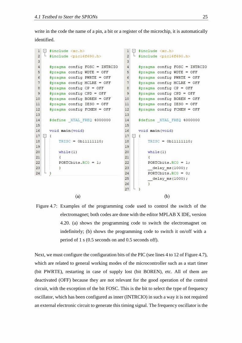
4.1 Testbed to Steer the SPIONs 25
write in the code the name of a pin, a bit or a register of the microchip, it is automatically
identified.
Figure 4.7: Examples of the programming code used to control the switch of the
electromagnet; both codes are done with the editor MPLAB X IDE, version
4.20. (a) shows the programming code to switch the electromagnet on
indefinitely; (b) shows the programming code to switch it on/off with a
period of 1 s (0.5 seconds on and 0.5 seconds off).
Next, we must configure the configuration bits of the PIC (see lines 4 to 12 of Figure 4.7),
which are related to general working modes of the microcontroller such as a start timer
(bit PWRTE), restarting in case of supply lost (bit BOREN), etc. All of them are
deactivated (OFF) because they are not relevant for the good operation of the control
circuit, with the exception of the bit FOSC. This is the bit to select the type of frequency
oscillator, which has been configured as inner (INTRCIO) in such a way it is not required
an external electronic circuit to generate this timing signal. The frequency oscillator is the

26 Chapter 4 Optimization of the Current System
circuit that indicates the speed with which the microcontroller works, and thus, it is an
essential component of all microprocessors or microcontrollers. It is a timing signal that
specifies the execution time of a programming instruction. Every four cycles or periods
(T) of this signal, an instruction of the programming code is executed. Therefore, if the
frequency (f) is configured as 4 MHz (see line 14 in Figure 4.7), each instruction will be
executed in 1 µs:
𝑡𝑖𝑚𝑒
𝑖𝑛𝑠𝑡𝑟𝑢𝑐𝑡𝑖𝑜𝑛= 4 · 𝑇 = 4 ·
1
𝑓= 4 ·
1
4 · 106 𝑠−1= 10−6 𝑠 = 1 µ𝑠 (4.2)
After the configuration of the bits and the definition of the frequency oscillator, comes
the main program. In line 18, the pin RC0 of the microcontroller is configured as an output
pin, since we use it to control the switch of the electromagnet. After that, Figure 4.7 shows
two alternatives: (a) switches the electromagnet on indefinitely; (b) switches it with a
period of 1 s (0.5 seconds on and 0.5 seconds off). During testing of the circuit together
with the rest of the setup we will test both programs. Also we will check different values
of switch period.
4.1.2.2 Transistor
Taking into account the maximum collector-emitter voltage (𝑉𝐶𝐸) at which the transistor
will be subjected and the maximum current (𝐼𝐶) that will flow through the electromagnet,
which are approximately 11 V and 167 mA, a transistor BC337-40 of type npn has been
chosen. It tolerates a maximum 𝑉𝐶𝐸 of 45 V and a maximum 𝐼𝐶 of 800 mA.
4.1.2.3 Rectifier Diode
The model selected as rectifier diode is the SDT20120CT, with a maximum DC blocking
voltage (𝑉𝑅𝑀) of 120 V and an average rectified output current (𝐼𝑂) of 20 A. This values
guarantee the good work of the component. The rectifier is connected parallel with
reversed polarity to the electromagnet in order to allow the flowing of current when the
transistor switches off. When it occurs, a very high voltage of opposite polarity is
generated in the terminals of the electromagnet. Thus, the rectifier absorbs this voltage
peak and protects the transistor.
4.1 Testbed to Steer the SPIONs 27
4.1.2.4 LED and Resistor
As informative indication of the activation of the electromagnet, a general red LED with
a DC forward current value (𝐼𝐹) of 2 mA and a forward voltage of 1.6-2 V has been
integrated in the circuit. A resistor of 500 Ω has been arranged in series with the LED in
order not to surpass its 𝐼𝐹 𝑚𝑎𝑥, which has a value of 30 mA.
4.1.2.5 Potentiometer
In the circuit, a potentiometer works as base resistance (𝑅B) of the BJT, which allows to
modify its resistance value according to the circuit necessities. These requirements are
the different values of 𝐼𝐶 that are needed in order to get different values of magnetic force
generated by the electromagnet. We want to test this circuit with the proposed testbed of
Figure 4.1, trying different values of magnetic force in order to check which one steers
the SPIONs most effectively.
To calculate 𝑅B, we need to know 𝐼𝐶, which is the sum of the current flowing through the
electromagnet plus the current flowing through the LED. This last current has an
approximately value of 2 mA (typical 𝐼𝐹 of the LED), much lower than the first one, thus,
it is considered negligible. 𝐼𝐶 is, then, the current flowing through the electromagnet.
Knowing that its 𝑅DC has a value of 66 Ω and employing Ohm’s law, we obtain different
values of 𝐼C according to the voltage 𝑉S used to source the electromagnet:
𝐼C =𝑉S𝑅DC
(4.3)
Next, the DC current gain (β) of the transistor is determined with a multimeter. It has a
value of 307 (dimensionless in SI units). Therefore, the current flowing through the base
of the transistor 𝐼B is:
𝐼B =𝐼Cβ=
𝐼C307
(4.4)
𝐼B is also the current flowing through the pinout of the microcontroller, which can have a
maximum value of 25 mA. If it is exceeded, the PIC could be damaged. As a protection
measure, the value obtained with equation 4.4 is multiplied by a security factor of 5.
Finally, the value of 𝑅B can be calculated using Ohm’s law:

28 Chapter 4 Optimization of the Current System
𝑅B =𝑉B𝐼B
𝑅B =𝑉pinout − 𝑉BE
𝐼B
𝑅B =5 V − 0.7 V
𝐼B
(4.5)
where 𝑉pinout is the voltage of the pinout of the microcontroller (approximately 5 V) and
𝑉BE is the base-emitter voltage, which is 0.7 V due to the transistor is made of silicon.
The results are shown in Table 4.2.
Table 4.2: Acquired values for the collector current 𝐼C and base current 𝐼B according
to the voltage supply of the electromagnet 𝑉S. Also the value of the base
resistor 𝑅B that is required for each situation. 𝐼C, 𝐼B and 𝑅B are calculated
with equations (4.3), (4.4) and (4.5), respectively.
𝑽𝐒 [V] 𝑰𝐂 [mA] 𝑰𝐁· 5 [mA] 𝑹𝐁 [Ω] commercial 𝑹𝐁 [Ω]
1 15 0.25 17425.3 18k
2 30 0.49 8712.7 8200
3 45 0.74 5808.4 5600
4 61 0.99 4356.3 4700
5 76 1.23 3485.1 3300
6 91 1.48 2904.2 2700
7 106 1.73 2489.3 2700
8 121 1.97 2178.2 2200
9 136 2.22 1936.1 1800
10 152 2.47 1742.5 1800
11 167 2.71 1584.1 1500
As we can see, the 𝐼B acquired (multiplied by a security factor 5) is lower than the
maximum allowed in the pinout of the microcontroller (25 mA). The values of 𝑅B
calculated with equation (4.5) have been rounded to values of commercial resistors, so
that it is easier to adjust the potentiometer. Furthermore, if it is desired in the future to use
the circuit with only a specific voltage supply of the electromagnet, then the potentiometer
can be replaced by a commercial resistor whose value is indicated in the table.
4.1 Testbed to Steer the SPIONs 29
It is considered that with 1 V the electromagnet will do no effect on the magnetic particles
due to a low magnetic force. Thus, neglecting the value of 18 kΩ, it is needed a
potentiometer that covers a value of resistance from 1500 to 8200 Ω. It has been selected
a general one with a maximum value of 10 kΩ.
4.1.3 Simulation of the Control Circuit
The circuit presented in the previous section has been simulated with the different values
of voltage source 𝑉S and commercial 𝑅B shown in Table 4.2. As Figure 4.8 shows, the
microcontroller is replaced by a DC voltage source of 5 V in the simulation, since this is
the value it gives approximately in its pinout. The LED and resistor R have been not taken
into account because they are only used as an informative indication and do not affect the
proper operation of the circuit. For that purpose, it has been used the simulation software
LTspice® (Linear Technology).
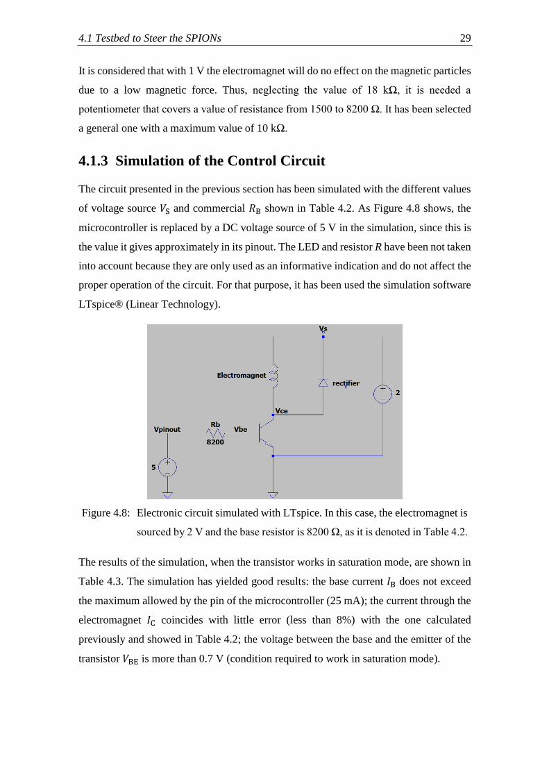
Figure 4.8: Electronic circuit simulated with LTspice. In this case, the electromagnet is
sourced by 2 V and the base resistor is 8200 Ω, as it is denoted in Table 4.2.
The results of the simulation, when the transistor works in saturation mode, are shown in
Table 4.3. The simulation has yielded good results: the base current 𝐼B does not exceed
the maximum allowed by the pin of the microcontroller (25 mA); the current through the
electromagnet 𝐼C coincides with little error (less than 8%) with the one calculated
previously and showed in Table 4.2; the voltage between the base and the emitter of the
transistor 𝑉BE is more than 0.7 V (condition required to work in saturation mode).

30 Chapter 4 Optimization of the Current System
Table 4.3: Acquired values from the simulation when the transistor works in saturation
mode (switched on), according to the voltage supply of the electromagnet
𝑉S: the collector current 𝐼C, the base current 𝐼B, the collector-emitter voltage
𝑉CE and the base-emitter voltage 𝑉BE.
𝑽𝐒 [V] 𝑰𝐂 [mA] 𝑰𝐁 [mA] 𝑽𝐂𝐄 [mV] 𝑽𝐁𝐄 [V]
2 28.63 0.50 110.63 0.86
3 43.76 0.74 112.04 0.87
4 58.85 0.88 115.95 0.88
5 74.06 1.25 112.06 0.89
6 89.22 1.52 111.65 0.89
7 104.29 1.52 116.65 0.90
8 119.48 1.86 114.46 0.90
9 134.67 2.28 111.93 0.90
10 140.77 2.28 115.31 0.90
11 164.96 2.73 112.61 0.91
4.1.4 Testing of the Control Circuit
Next step is doing testing with the designed circuit. For that purpose, the testbed shown
in Figure 4.9 has been used. We want to check the proper operation of the circuit for each
voltage value that sources the electromagnet.
Figure 4.9: Testbed used to check the functioning of the control circuit to switch the
electromagnet.

4.1 Testbed to Steer the SPIONs 31
The circuit has been tested with a cyclical switch of 8 seconds (4 seconds on and 4 seconds
off), but only the results when the transistor is working in saturation mode (switched on)
are presented in Table 4.4. When the transistor works in cut-off mode (switched off), no
current flows through the electromagnet, thus, no magnetic force is generated. It has been
checked that the rectifier works properly and absorbs the voltage peak produced by the
electromagnet when it is switched off almost immediately.
Table 4.4: Acquired values from the testing when the transistor works in saturation
mode (switched on), according to the voltage supply of the electromagnet
𝑉S: the voltage of the pinout of the microcontroller 𝑉pinout, the collector
current 𝐼C, the base current 𝐼B, the collector-emitter voltage 𝑉CE and the
base-emitter voltage 𝑉CE.
𝑽𝐒 [V] 𝑽𝐩𝐢𝐧𝐨𝐮𝐭 [V] 𝑰𝐂 [mA] 𝑰𝐁 [mA] 𝑽𝐂𝐄 [mV] 𝑽𝐁𝐄 [V]
2 5.00 28.19 0.52 51.75 0.71
3 4.98 41.70 0.75 59.20 0.73
4 4.97 55.60 0.90 70.07 0.74
5 4.95 69.50 1.27 73.30 0.75
6 4.94 83.90 1.54 82.34 0.76
7 4.94 95.40 1.54 94.30 0.76
8 4.92 110.40 1.87 97.88 0.77
9 4.90 122.40 2.27 104.30 0.78
10 4.90 133.80 2.28 112.10 0.78
11 4.88 148.70 2.70 118.34 0.79
As we can see in the table above, the output voltage sourced by the microcontroller in its
pinout keeps approximately 5 V for each value of 𝑉S. The obtained base current 𝐼B is
much less than 25 mA (the maximum allowed) and differs maximum a 4% from the one
obtained in simulation; the collector current differs less than 10%. These results are good,
since we had applied a security factor of 5 when we have determined the values of the
base resistor (potentiometer) in section 4.1.2.5 of this document. Therefore, there is a big
margin of error. Furthermore, acquired values of 𝑉CE and 𝑉CE confirm that the transistor
is working properly in saturation mode. The LED emits light for each situation of the
table and the electromagnet attracts a paperclip when is switched on, thus, it is confirmed
that a magnetic force is generated.

32 Chapter 4 Optimization of the Current System
In next section, the electronic circuit is tested together with the molecular testbed
developed by FAU in order to check if the electromagnet affects the SPIONs trajectory

Chapter 5
Results and Discussion
A
After having confirmed that the designed circuit to control the switch of the electromagnet
works properly, it has been tested together with the rest of the setup. Two rounds of testing
have been conducted: the first one without susceptometer in order to acquire a qualitative
view of the efficacy of the electromagnet in the system operation; a second one with
susceptometer in order to obtain accurate results.
5.1 Testing without Susceptometer
The whole testbed we want to test, which is showed in Figure 4.1 from section 4.1,
contains many variables that could affect the behaviour of the SPIONs whereas they are
flowing in the system. These variables are the voltage source of the electromagnet (𝑉S),
the switch period of the electromagnet (T, configured in the programming code), the flow
rate pumped (Q), the position of the electromagnet in the testbed, and the ratio SPIONs
and water used in the injected mixture.
A first round of testing has been accomplished, in which the susceptometer has not been
used (see Figure 5.1). Because of that, we can not determine with accuracy if more
magnetic particles are steered through the desired path after the Y-connector due to the
influence of the electromagnet, but we acquire a qualitative view of the general operation
of the system.

34 Chapter 5 Results and Discussion
Figure 5.1: Testbed used for experiments without susceptometer.
For this testing, the mixture of SPIONs and water has been fixed as 1 mL of SPIONs plus
1 mL of water in order not to have many variables. This mixture is pumped towards the
Y-connector, near which the electromagnet is located. Finally, the particles and water are
collected in a waste container.
For the electromagnet positioning, two rulers with cm scale have been incorporated, being
the position (x, y) = (0, 0) the beginning of the split (see Figure 5.2). The electromagnet
is also placed in such a way that its longitudinal axis crosses the tubes where the SPIONs
are flowing.
(a) (b)
Figure 5.2: (a) Rulers with cm scale to reference the location of the electromagnet in
the testbed. Position (x, y) = (0, 0) is the start of the Y-connector. (b) Front
view of the electromagnet located in the setup.

5.1 Testing without Susceptometer 35
A multimeter has been used to verify the resistance value selected with the potentiometer
(𝑅B). Since it is a handmade operation and it is difficult to get an identical value as the
indicated in Table 4.2 (commercial 𝑅B), we consider good resistance values those with a
margin of ±10 Ω. Thus, if the value of 𝑅B must be 1500 Ω, but we get one of 1490 or
1510 Ω with the potentiometer, then it is considered correct. It is reasonable since we
have applied a security factor of 5 when we have determined the required values of base
resistor according to the voltage supply of the electromagnet in section 4.1.2.5, thus, it
does not affect the proper working of the control circuit of the electromagnet.
In this testing several values of the different variables of the system has been used:
The next pumped flow rates Q in mL/min: 0.5, 1, 2, 3 and 4.
The next positions (x, y) in cm for the electromagnet: (1, 0), (1.5, 0), (2, 0) and
(0, 0.7) being x the position of the longitudinal axis of the component.
Figure 5.3: Electromagnet in position (1,0) cm.
The next voltage sources of the electromagnet 𝑉S in volts: 2, 3, 4, 5, 6, 7, 8, 9, 10,
11.
The next switch periods T of the electromagnet in seconds: 0.1, 0.5, 1, 2, 4. Also,
it has been tested with the electromagnet switched on indefinitely.
As illustrated in Figure 5.4, the mixture of SPIONs and water flow through both channels
after the Y-connector without the influence of a magnetic field generated by the
electromagnet.

36 Chapter 5 Results and Discussion
Figure 5.4: Testbed working without the electromagnet. As a result, the mixture of
SPIONs and water flows through both channels after the Y-connector.
First, it has been tested with the electromagnet switched on indefinitely and different
combination of the rest of variables. In all cases, it has been observed the same
performance: when the mixture arrives at the area where the electromagnet is located, the
particles are attracted to the walls of the tube (see Figure 5.5) and then, they start to flow
through the desired path (correct path) after the Y-connector.
Figure 5.5: Mixture flowing through the desired path after the Y-connector. It can be
appreciated how the SPIONs are attracted to the border of the tube near
the electromagnet. Flow rate Q = 0.5 mL/min; voltage source of the
electromagnet 𝑉S = 11 V; electromagnet in position (1,0) cm;
electromagnet switched on indefinitely.
After some seconds, it seems they agglomerate near the electromagnet, which block the
proper flow through the correct path and they begin to flow in both channels (see Figure
5.6).

5.1 Testing without Susceptometer 37
Figure 5.6: Mixture flowing through both channels after the Y-connector. Flow rate
Q = 0.5 mL/min; voltage source of the electromagnet 𝑉S = 11 V;
electromagnet in position (1, 0) cm; electromagnet switched on
indefinitely.
After the particles have started to flow through the desired way, the maximum time it
takes to them to start to flow through both channels (t) is approximately 30 seconds, for
a flow rate Q of 0.5 mL/min. This time decreases as greater is Q, obtaining one of
approximately 8 seconds for a flow rate of 4 mL/min and sourcing the electromagnet with
2 V. Placing the electromagnet in position (0, 0.7) cm (see Figure 5.7), (1.5, 0) cm or (2,
0) cm, acquired results are worse (shorter t).
Figure 5.7: Electromagnet in position (0, 0.7) cm.
Finally, it has been observed the shorter the switch period of the electromagnet is, better
results are acquired (greater t). It could be on account of a less agglomeration of the
particles (during the switch on, the electromagnet attracts the particles; during the switch
off, they flow freely). The best obtained results are with a switch period of 200 ms (100
ms on and 100 ms off, cyclically). In this situation, the greatest t is 1 min for a flow rate
of 0.5 mL/min.

38 Chapter 5 Results and Discussion
Thus, for the moment, we can conclude that the best position of the electromagnet to work
more effectively is (1, 0) cm; the lower is the flow rate Q, better results are acquired and
short switch periods of the electromagnet are better. Anyway, these results are qualitative
since a susceptometer has not been used. In next section, accurate results of testing using
this device are presented.

5.2 Testing using a Susceptometer 39
5.2 Testing using a Susceptometer
In next testing, a MS2G Bartington® susceptometer coil (inner diameter: 10 mm, height:
5 mm) has been employed in order to determine with precision the effectiveness of the
magnetic field on SPIONs. A susceptometer is an electronic device including a coil,
where the magnetic particles move through and generate an electrical signal 𝜒(t). This
signal is proportional to the number of SPIONs that are within the detection range at a
specific time instance. Susceptibility changes measured are recorded by use of the
software Bartsoft 4.2.1.2 (Bartington Instruments, Witney, UK) provided by the
manufacturer of the susceptometer. For that purpose, the testbed shown in Figure 5.8 has
been used.
Figure 5.8: Testbed used to check the efficacy of the magnetic field generated by an
electromagnet to steer SPIONs through a molecular communication
system.
All tubes have an inner diameter of 0.8 mm, both channels after the Y-connector have the
same length and are positioned symmetrically.
In order to guarantee equal flow conditions in both channels after the splitting, two pumps
in parallel have been used, one for each channel. The two pieces shown in Figure 5.9 have
been used to get identical parallel flows with the same pump. In this way, the flow rate
acquired in the tube placed between the glass with SPIONs and the start of the splitting

40 Chapter 5 Results and Discussion
(flow rate Q), is the sum of the flow rates of both channels after the Y-connector.
(a) (b)
Figure 5.9: (a) Pieces used to get equal parallel flows in both channels after the Y
connector. (b) Photograph where we can see how the mixture flows at the
same time through both ways.
The purpose is to measure the magnetic susceptibility of both paths after the Y-connector
in order to see if there is a difference between them. In particular, a greater value in the
desired path than the other one is expected, since more SPIONs in the first way are
supposed to flow due to the influence of the magnetic field.
The ideal would be to use two susceptometers, so that the magnetic susceptibilities of
both channels were measured at the same time. Nevertheless, FAU can only provide one
device. For that reason, the next procedure has been accomplished:
1. First, the magnetic susceptibility has been measured without using the
electromagnet in the system. In this way, a baseline is acquired. For this operation,
the susceptometer can be placed in any of two channels, since there is no magnetic
field generated and, thus, SPIONs flow equally through both tubes (see Figure
5.10).

5.2 Testing using a Susceptometer 41
Figure 5.10: Susceptometer positioned in one of the channels in order to acquire a
magnetic susceptibility baseline. For this operation the electromagnet is
not used.
2. Next step is activating the control circuit of the electromagnet and measuring of
magnetic susceptibility in one of the channels, as illustrated in Figure 5.11.
Figure 5.11: Measuring of magnetic susceptibility changes in one of the channels with
the electromagnet activated. In this case, the device is positioned in the
desired path (correct path), where the SPIONs are supposed to flow with
larger proportion than in the other path (incorrect path) due to the effect
of the magnetic field.
3. Finally, measuring of magnetic susceptibility changes in the other channel are
registered, being also the electromagnet switched on.
In steps 2 and 3, the susceptometer has been placed at the same areas in respective
channels, so that the measuring conditions were as similar as possible. Also, the start of
each measuring round has been done as soon as the mixture of SPIONs and water reaches
the red line shown in Figure 5.12.

42 Chapter 5 Results and Discussion
Figure 5.12: Susceptometer location in the testbed. When the particles reach the red
line, then the susceptometer start to measure the magnetic susceptibility
changes.
A total number of 1000 samples every 0.1 seconds (in total, 100 seconds) have been
registered for each measurement round. Finally, after the particles have passed through
the susceptometer and the pump, they are collected in a waste container in order to be
reused.
The next values for the different variables of the system have been used:
Table 5.1: Values of the different variables that have been tested during experiments
with the setup using a susceptometer.
Variable Values
Flow rate Q [mL/min] 0.752, 1, 2, 3, 4
Electromagnet voltage source Vs [V] 2, 6, 11
Electromagnet position (x, y) [cm] (1, 0), (1.5, 0), (0, 0.8)
Electromagnet switch period T [s] 0.01, 0.1, 0.5, 2
Mixture (mL SPIONs, mL water) (1, 2), (1, 4)
SPIONs with a hydrodynamic particle radius of 27.5 nm are used. The electromagnet
positions indicated in the table above are shown in Figure 5.13, being the position (0, 0)
the start of the Y-connector; x coordinate corresponds to the longitudinal axis position of
the electromagnet; y coordinate is the position of the electromagnet front face.

5.2 Testing using a Susceptometer 43
(a) (b) (c)
Figure 5.13: Electromagnet positions tested during experiments with susceptometer.
x coordinate is the position of the electromagnet longitudinal axis; y
coordinate is the position of the electromagnet front face. (a) Position
(1, 0) cm. (b) Position (1.5, 0) cm. (c) Position (0, 0.8) cm.
The procedure previously mentioned has been accomplished with different combinations
of these variables. The results are shown in next section.
5.2.1 Results of testing using a Susceptometer
In all the experiments it has not been possible to visualize directly if the electromagnet
does any effect to SPIONs trajectory. As illustrated in Figure 5.14, the particles have
flowed through both channels for all the combinations tested in this work.
Figure 5.14: Behaviour of the magnetic particles observed in all measuring rounds
during testing with susceptometer. The mixture of SPIONs and water
flows through both channels, not allowing to visualize any effect on
SPIONs. In the present photograph: electromagnet is switched on
indefinitely; Q = 1 mL/min; electromagnet in position (1, 0) cm; Vs = 11
V; mixture (1, 2) mL.

44 Chapter 5 Results and Discussion
First, a mixture of 1 mL of SPIONs plus 2 mL of water has been used. Results of a first
round using Vs = 11 V, being the electromagnet switched on indefinitely and positioned
in (1, 0) cm are shown in Figure 5.15.
Figure 5.15: Acquired measurements of magnetic susceptibility in both channels after
the Y-connector according to different values of flow rate. Mixture (1, 2)
mL; Voltage source of the electromagnet Vs = 11 V; electromagnet placed
in position (1,0) cm. baseline (red) Q = 0.752 (dark blue)
aaaaaQ = 1 (green) Q = 2 (brown) Q = 3 (yellow) Q = 4
(soft blue). All flow rates in mL/min.
As we can observe, only with a flow rate of 1 mL/min (green) there is an increase in the
correct path compared to the baseline, although it is insignificant (the magnetic
susceptibility values have the same order and differ less than 5×10⁻⁵ units). Also, acquired
measurements in the incorrect path show an insignificant decrease of magnetic
susceptibility compared to the baseline.
Next, keeping a Vs = 11 V, different positions of the electromagnet have been tested (see
Figure 5.16). Although the differences are also not significant, we observe that only for
position (0, 1) cm the susceptibilities have increased with the except of that for 0.752
mL/min. We proceed, thus, to use this electromagnet position in next rounds.

5.2 Testing using a Susceptometer 45
Figure 5.16: Acquired measurements of magnetic susceptibility in the correct channel
according to different values of flow rate and position of the
electromagnet. Mixture (1, 2) mL; Voltage supply of the electromagnet
Vs = 11 V. baseline (red) Q = 1 (green) Q = 2 (brown)
aaaaaQ = 3 (yellow) Q = 4 (soft blue). All flow rates in mL/min.
Electromagnet position
(1, 0) cm
Electromagnet position
(1.5, 0) cm
Electromagnet position
(0, 0.8) cm

46 Chapter 5 Results and Discussion
In the following, the efficacy of the switch period of the electromagnet (T) has been
checked (see Figure 5.17). For that purpose, a flow rate of 1 mL/min has been used
because of the better results acquired with such value in previous experiments shown in
Figure 5.15.
Figure 5.17: Acquired measurements of magnetic susceptibility in the correct channel
according to different values of switch period of the electromagnet (T).
Mixture (1, 2) mL; Voltage supply of the electromagnet Vs = 11 V;
electromagnet in position (1, 0) cm; flow rate Q = 1 mL/min. baseline
(red) T = 0.01 s (brown) T= 0.1 s (green) T = 0.5 s (dark
blue) T = 2 s (yellow).
The results shown in the figure above indicate there is no difference among the different
switch periods. The differences are insignificant, thus, we use the electromagnet switched
on indefinitely for next measuring rounds.
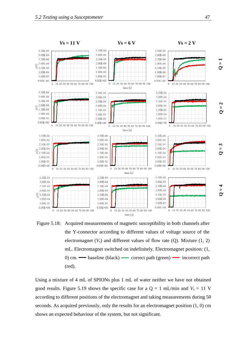
Finally, the results acquired according to the different values of the electromagnet voltage
supply Vs and flow rates Q are illustrated in Figure 5.18. Although the differences among
the magnetic susceptibility of both channels and the baseline are no significant in all
cases, we observe that higher voltage sources (Vs = 11 V) and lower flow rates (Q =1
mL/min) approaches more to the initial expected results (an increase of magnetic
susceptibility in the correct path and a decrease in the other one). On the other hand, we
conclude that lower Vs (6 and 2 V) and higher Q (2, 3 and 4 mL/min) yield bad results.
For that situations, the measurement in the incorrect path is higher than the correct path,
which is contrary to expected.
5.2 Testing using a Susceptometer 47
Figure 5.18: Acquired measurements of magnetic susceptibility in both channels after
the Y-connector according to different values of voltage source of the
electromagnet (Vs) and different values of flow rate (Q). Mixture (1, 2)
mL. Electromagnet switched on indefinitely. Electromagnet position: (1,
0) cm. baseline (black) correct path (green) incorrect path
(red).
Using a mixture of 4 mL of SPIONs plus 1 mL of water neither we have not obtained
good results. Figure 5.19 shows the specific case for a Q = 1 mL/min and Vs = 11 V
according to different positions of the electromagnet and taking measurements during 50
seconds. As acquired previously, only the results for an electromagnet position (1, 0) cm
shows an expected behaviour of the system, but not significant.
Vs = 11 V Vs = 6 V Vs = 2 V
Q =
1
Q =
2
Q =
3
Q =
4

48 Chapter 5 Results and Discussion
Figure 5.19: Acquired measurements of magnetic susceptibility in both channels after
the Y-connector according to different positions of the electromagnet.
Mixture (1, 4) mL; Vs = 11 V; flow rate Q = 1 mL/min. Electromagnet
switched on indefinitely. baseline (black) correct path (green)
aaaaaincorrect path (red).
Because of these bad results, we have also decided to test with the setup shown in Figure
5.1 from section 5.1 (Testing without Susceptometer), where it is used only one pump
and the qualitative results showed that the magnetic field generated by the electromagnet
affect the trajectory of the SPIONs, but now adding the susceptometer. Nevertheless,
results show again an insignificant difference among measurements of the channels (see
Figure 5.20).

5.2 Testing using a Susceptometer 49
Figure 5.20: Acquired measurements of magnetic susceptibility in both channels after
the Y-connector according to different positions of the electromagnet.
Mixture (1, 4) mL; Vs = 11 V; flow rate Q = 1 mL/min. Electromagnet
switched on indefinitely. baseline (black) correct path (green)
aaaaaincorrect path (red).
The no significant results acquired with the previous combination of variables of the
system suggest this electromagnet does not generate enough magnetic force to affect the
magnetic particles trajectory; another one with higher force is required. Even then, we
could observe how the results approximates more to the expected ones with higher voltage
source of the electromagnet Vs (11 V), which means higher magnetic forces. Also, with
lower flow rates (Q = 1 mL/min) and positioning the electromagnet in (1, 0) cm.
5.2.2 Problems during Testing
In this section we explain briefly the problem we have had during the realized
experiments and its possible relation with the results acquired. In this way, a better
measuring procedure can be accomplished in future research work.
The main problem has been the precipitation of the SPIONs. As Figure 5.21 shows, the
SPIONs on the left glass are precipitated, which implies they are agglomerated. This is
the state at which the nanoparticles are when they have been mixed, for instance, with
non-distilled water or other chemical substance. In accomplished testing in this work,
oxalic acid has been used in order to remove from the tubes of the testbed any residual
particle after each measuring round. If the tubes are not cleaned with proper amount of
distilled water after the oxalic acid has flowed through them, it is likely it mixes with
SPIONs at next measuring round, causing its precipitation.

50 Chapter 5 Results and Discussion
Figure 5.21: Glasses with mixtures of SPIONs and water. On the left, a glass with
precipitated SPIONs; on the right, a glass with SPIONs in proper state to
be used in testing.
This phenomenon has been produced in some of the measurements, causing that the
particles agglomerate and stick on the walls of the tubes (see Figure 5.22). When this
occurs, the flow of SPIONs can be block, causing failed measurements of magnetic
susceptibility.
(a) (b)
Figure 5.22: Precipitation of SPIONs during the testing. (a) SPIONs precipitate and
consequently, they are agglomerated. (b) Zoom in of red circle from (a).
Precipitated SPIONs tend to stick on the walls of the tubes not allowing
the proper flow of the mixture.
Thus, in future research studies of the presented work, it is totally required to ensure that
the tubes do not contain residual components like acids or non-distilled water in order to
conduct reliable experiments with the magnetic particles.

Chapter 6
Conclusion and Outlook
A
6.1 Conclusion
As part of this thesis, an optimization of the transmitter setup of a molecular
communication testbed based on superparamagnetic iron nanoparticles in duct flow has
been developed. For that purpose, the magnetic field generated by an electromagnet has
been used in order to try to steer the magnetic particles through a desired path after a Y-
connector.
An electromagnet whose size is in proportion to the tubes used in the system has been
selected. It has been placed in different positions in the proximity of the splitting, as well
as different combinations of other variables of the system have been tested. These
variables are the amount of SPIONs and water used in the injected mixture, the flow rate
pumped, the voltage supply of the electromagnet and the switch period of the
electromagnet. SPIONs with a particle radius of 27.5 nm have been used.
The efficacy of the proposed testbed has been determined measuring magnetic
susceptibility changes in both channels after the Y-connector. For this operation, only a
susceptometer coil provided by FAU has been used. The ideal procedure would have been
to use two devices, so that magnetic susceptibilities in the channels were measured at the
same time. In this way, acquired measurements would be more reliable.
For each injection mixture used, a magnetic susceptibility baseline has been registered,
which has consisted in measuring the magnetic susceptibility of the system without using
the electromagnet. The expected behaviour of the magnetic particles under the influence
of the electromagnet was the next: an increase of the magnetic susceptibility in the desired

52 Chapter 6 Conclusion and Outlook
path after the Y-connector compared to the baseline, where more SPIONs than in the
other channel are supposed to flow; on the other hand, a decrease of magnetic
susceptibility in the other path.
Experimental results have shown a no expected performance of the system: there is no
significant difference among magnetic susceptibilities of both channels and the baseline,
neither between both channels. Thus, the magnetic field generated by this electromagnet
does not affect the SPIONs trajectory. Even then, acquired results have been closer to the
expected ones for a combination of higher voltages sources of the electromagnet
(specifically 11 V), which indicates that another electromagnet with higher magnetic
force is required. Also, results have been closer for lower flow rates (specifically 1
mL/min) and positioning the electromagnet in such next way: its front face contacting the
walls of the tube; its longitudinal axis oriented perpendicularly to the tube and positioned
at a distance of 1 cm from the start of the Y-connector.
Furthermore, we have had a big problem during the experiments. The magnetic
nanoparticles have been precipitated after they have been used some attempts, which has
implied the need to repeat some of the measurements. That phenomenon can be related
to the fact that we have used oxalic acid to clean the tubes after each measuring round.
This acid may have been mixed together with SPIONs if it has not been used enough
distilled water to remove residual particles of that acid and, thus, causing its precipitation.
It can also be caused if SPIONs are mixed with non-distilled water. Therefore, in future
research work it should be ensured this phenomenon does not occur in order to get more
reliable results.
Summarizing, results denote that an electromagnet with higher magnetic field should be
selected as well as new experiments should be conducted using new combinations of the
variables of the system. Experimentation with larger SPIONs is also suggested. For that
purpose, it has been confirmed that FAU can provide SPIONs of approximately 100 nm
in the future.
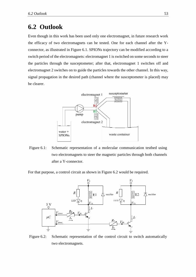
6.2 Outlook 53
6.2 Outlook
Even though in this work has been used only one electromagnet, in future research work
the efficacy of two electromagnets can be tested. One for each channel after the Y-
connector, as illustrated in Figure 6.1. SPIONs trajectory can be modified according to a
switch period of the electromagnets: electromagnet 1 is switched on some seconds to steer
the particles through the susceptometer; after that, electromagnet 1 switches off and
electromagnet 2 switches on to guide the particles towards the other channel. In this way,
signal propagation in the desired path (channel where the susceptometer is placed) may
be clearer.
Figure 6.1: Schematic representation of a molecular communication testbed using
two electromagnets to steer the magnetic particles through both channels
after a Y-connector.
For that purpose, a control circuit as shown in Figure 6.2 would be required.
Figure 6.2: Schematic representation of the control circuit to switch automatically
two electromagnets.

54 Chapter 6 Conclusion and Outlook
Because of a new electromagnet with higher magnetic force is required for future
experiments and it is likely to allow a different range of voltage supply Vs, the base
resistor of the control circuit must be recalculated, according to the procedure followed
in section 4.1.2.5 of this document.
In Figure 6.3, we present an example of the programming code to control automatically
the switch of both electromagnets.
Figure 6.3: Programming code to switch cyclically two electromagnets using the
editor MPLAB X IDE. The microcontroller controls the switch of both
electromagnets by pins RC0 and RC1.
One electromagnet receives the signal from the microcontroller by pin RC0 and the other
one by pin RC1. Different values of switch period can be tested changing the number of
delay commands (lines 26, 29, 32 and 35 in the programming code).

Appendix A
Appendix
A
The enclosed CD-ROM includes following data:
Datasheets of the components used in the control circuit to switch the
electromagnet
Simulation file of the control circuit for LTspice®
Magnetic susceptibility measurements acquired during testing
Programming codes for the microcontroller:
- To switch an electromagnet on indefinitely
- To switch an electromagnet on/off cyclically
- To switch two electromagnets on/off cyclically
Recorded videos during testing
Master thesis: Optimization of the transmitter setup for a molecular
communication link based on superparamagnetic iron nanoparticles, by Carlos
Martínez Cantón

List of Figures
A
2.1 Schematic representation of molecular communication between a
transmitter and a receiver……………………………………………………
4
2.2 Schematic representation of magnetic dipoles of a paramagnetic material
under the influence of an applied magnetic field gradient…………………...
7
2.3 Magnetization curves for ferromagnetic, paramagnetic and
superparamagnetic materials..........................................................................
8
2.4 Magnetic particle with coating……………………………………………… 10
2.5 Magnetic field lines generated by solenoids and electromagnets…………… 11
2.6 Schematic of the steering of a SPION through a specific path by the
influence of the magnetic field generated by an electromagnet……………...
13
3.1 Photograph of the molecular communication system developed by FAU….. 15
3.2 Photograph of the Y-connector……………………………………………... 16
4.1 Schematic representation of the testbed proposed to check the efficacy of a
magnetic field on SPIONs…………………………………………………...
19
4.2 Activated electromagnet near a plastic glass with a mixture of SPIONs and
water………………………………………………………………………...
21
4.3 Schematic of an electromagnet supplied with a DC voltage source…………. 21
4.4 Schematic of the electronic circuit used to control the switch of the
electromagnet…………………………………………………….................
22
4.5 Electronic circuit to control automatically the switch of the electromagnet
mounted on a protoboard…………………………………………………….
23
4.6 PIC16F690 pin diagram…………………………………………………….. 24
4.7 Examples of the programming code used to control the switch of the
electromagnet……………………………………………………………….
25
4.8 Electronic circuit simulated with LTspice………………………….………. 29
4.9 Testbed used to check the functioning of the control circuit to switch the
electromagnet……………………………………………………………….
30
5.1 Testbed used for experiments without susceptometer……………………… 34
5.2 Rulers with cm scale to reference the location of the electromagnet in the
testbed. Front view of the electromagnet located in the setup………………
34
5.3 Electromagnet in position (1,0) cm…………………………………………. 35
5.4 Testbed working without the electromagnet………………………………... 36

58 List of Figures
5.5 Mixture flowing through the desired path after the Y-connector…………… 36
5.6 Mixture flowing through both channels after the Y-connector……………... 37
5.7 Electromagnet in position (0, 0.7) cm………………………………………. 37
5.8 Testbed used to check the efficacy of the magnetic field generated by an
electromagnet to steer SPIONs through a molecular communication
system……………………………………………………………………….
39
5.9 Pieces used to get equal parallel flows in both channels after the Y
connector……………………………………………………………………
40
5.10 Susceptometer positioned in one of the channels in order to acquire a
magnetic susceptibility baseline………………………………………...…..
41
5.11 Measuring of magnetic susceptibility changes in one of the channels with
the electromagnet activated………………………………………………….
41
5.12 Susceptometer location in the testbed…………………………...………….. 42
5.13 Electromagnet positions tested during experiments with susceptometer…… 43
5.14 Behaviour of the magnetic particles observed in all measuring rounds during
testing with susceptometer…………………………………………………..
43
5.15 Acquired measurements of magnetic susceptibility in both channels after the
Y-connector according to different values of flow rate……………………..
44
5.16 Acquired measurements of magnetic susceptibility in the correct channel
according to different values of flow rate and position of the electromagnet
45
5.17 Acquired measurements of magnetic susceptibility in the correct channel
according to different values of switch period of the electromagnet…………
46
5.18 Acquired measurements of magnetic susceptibility in both channels after the
Y-connector according to different values of voltage source of the
electromagnet and different values of flow rate……………………………..
47
5.19 Acquired measurements of magnetic susceptibility in both channels after the
Y-connector according to different positions of the electromagnet…………
48
5.20 Acquired measurements of magnetic susceptibility in both channels after the
Y-connector according to different positions of the electromagnet…………
49
5.21 Glasses with mixtures of SPIONs and water………………………………... 50
5.22 Precipitation of SPIONs during the testing…………………………………. 50
6.1 Schematic representation of a molecular communication testbed using two
electromagnets to steer the magnetic particles through both channels after a
Y-connector…………………………………………………………………
53
6.2 Schematic representation of the control circuit to switch automatically two
electromagnets………………………………………………………………
53
6.3 Programming code to switch cyclically two electromagnets using the editor
MPLAB X IDE……………………………………………………………...
54

List of Tables
A
4.1 ITS-MS-2015 electromagnet parameters…………………………………… 20
4.2 Acquired values for the collector current and base current according to the
voltage supply of the electromagnet…………………………………………
28
4.3 Acquired values from the simulation when the transistor works in saturation
mode, according to the voltage supply of the electromagnet………………..
30
4.4 Acquired values from the testing when the transistor works in saturation
mode, according to the voltage supply of the electromagnet ……………….
31
5.1 Values of the different variables that have been tested during experiments
with the setup using a susceptometer………………………………………...
42

Bibliography
[1] N. Farsad, H. B. Yilmaz, A. Eckford, C.-B. Chae, and W. Guo, “A comprehensive
survey of recent advancements in molecular communication”, IEEE Commun.
Surv. Tutorials, vol. 18, no. 3, pp. 1887–1919, 2016.
[2] H. Unterweger, J. Kirchner, W. Wicket, A. Ahmadzadeh, D. Ahmed, V. Jamali,
C. Alexiou, G. Fischer, R. Schober, “Experimental Molecular Communication
Testbed Based on Magnetic Nanoparticles in Duct Flow”, 2018 IEEE 19th
International Workshop on SPAWC, pp. 1-5, 2018.
[3] Q. A. Pankhurst, J. Connolly, S. Jones, and J. Dobson, “Applications of magnetic
nanoparticles in biomedicine”, J. Phys. D: Appl. Phys., vol. 36, no. 13, p. R167,
2003.
[4] N. Farsad, W. Guo, and A. W. Eckford, “Tabletop molecular communication:
Text messages through chemical signals”, PLoS ONE, vol. 8, no. 12, p. e82935,
Dec. 2013.
[5] A. Ahmadzadeh, V. Jamal, W. Wicke, R. Schober, “Molecular Communication:
State-of-the-Art and Challenges”, Institute for Digital Communications of
Friedrich Alexander Universität Erlangen-Nürnberg, Kick-off Workshop for EFI
Project on Molecular Communication.
[6] R. S. M. Rikken, R. J. M. Nolte, J. C. Maan, J. C. M. Van Hest, D. A. Wilson, P.
C. M. Christianen, ”Manipulation of micro- and nanostructure motion with
magnetic fields”, Institute of Molecules and Materials, Radboud University
Nijmegen, The Netherlands, 2013.
[7] NPTEL, Modulea6:aMagneticaCeramics, Paramagnetism,
https://nptel.ac.in/courses/113104005/lecture30a/30_3.htm [Online; accessed on
10/10/2018]
[8] M.aMarolt, Superparamagneticamaterials, http://mafija.fmf.uni-
lj.si/seminar/files/2013_2014/superparamagnetic_materials.pdf [Online; accessed
on 18/09/2018].
[9] R. V. Ramanujan, MagneticaParticlesaforaBiomedicalaApplications,
http://www3.ntu.edu.sg/home/ramanujan/reprints/Bio%20book%20chapter.pdf
[Online; accessed on 19/09/2018].
[10] M.aMarolt, Superparamagnetism, http://eng.libretexts.org/Textbook-
Maps/Chemical_Engineering/Supplemental_Modules_(Materials_Science)/Mag
netic_Properties/Superparamagnetism [Online; accessed on 18/09/2018].
[11] D. M. Martín, Development of Nanofiber SPION Supports and Arsenic Speciation
Using Synchrotron and Hyphenated Techniques,

62 Bibliography
https://ddd.uab.cat/pub/tesis/2013/hdl_10803_129335/dmm1de1.pdf [Online;
accessed on 07/10/2018].
[12] Wahajuddin, S. Arora, “Superparamagnetic iron oxide nanoparticles: magnetic
nanoplatforms as drug carriers”, NCBI International Journal of Nanomedicine,
vol. 7, pp. 3445-3471, 2012.
[13] E. Carenza, Engineering Iron Oxide Nanoparticles For Angiogenic Therapies,
https://ddd.uab.cat/pub/tesis/2014/hdl_10803_284861/ec1de1.pdfa[Online; acce-
-sed on 07/10/2018].
[14] Electromagnet,ahttp://electromagnetismotelecouax2013.blogspot.com/2013/05/e
lectroiman.html [Online; accessed on 04/07/2018].
[15] L. C Barnsley, D. Carugo, J. Owen, E. Stride, “Halbach arrays consisting of
cubic elements optimised for high field gradients in magnetic drug targeting
applications”, IOP Science, Physics in Medicine & Biology, vol. 60, no. 21,
2015.
[16] S. S. Shevkoplyas, A. C. Siegel, R. M. Westervelt, M. G. Prentissc, G. M.
Whitesides, “The force acting on a superparamagnetic bead due to an applied
magnetic field”, NCBI, PubMed, 2007.
[17] Microchip, PIC16F690 Datasheet: PIC16F690 Pin Diagram, page 6,
https://www.microchip.com/wwwproducts/en/PIC16F690 [Online; accessed on
05/06/2018].