Implementation of Unified Model based Analysis-Forecast System … · 2012-07-12 · which is a special one used at Met Office. Proprietary software IDL (Interactive Data Language)

0

Implementation of Unified Model based

Analysis-Forecast System at NCMRWF

E.N. Rajagopal, G.R. Iyengar, John P. George, Munmun Das Gupta, Saji Mohandas, Renu Siddharth, Anjari Gupta, Manjusha Chourasia,

V.S. Prasad, Aditi, Kuldeep Sharma and Amit Ashish

May 2012

This is an Internal Report from NCMRWF. Permission should be obtained from the NCMRWF to quote from this report.

NMRF/TR/2/2012

TEC

HN

ICA

L R

EPO

RT

National Centre for Medium Range Weather Forecasting Ministry of Earth Sciences

A-50, Sector 62, NOIDA – 201309, INDIA

TEC

HN

ICA

L R

EPO

RT

1

Summary

A MoU was signed between MoES and Met Office, UK in August 2008, to collaborate

for developing a seamless numerical modelling system for prediction over different time ranges and spatial scales. The initial focus of this collaboration is on implementation of Met Office Unified Model (UM) global forecast suite at NCMRWF which includes atmospheric modelling and data assimilation.

Under this initiative Unified Model (UM) based a global analysis-forecast system at N512L70 resolution has been implemented at NCMRWF on IBM HPC. A description of the various components of this UM global forecast suite is attempted in this report. The implementation strategy adopted at NCMRWF is also described in detail. Some sample results from this system are also presented.

2

Contents

1. Introduction 3 2. Components of the UM global forecast suite 3

3. Prerequisites for implementing the UM global forecast suite 3

4. Implementation Process at NCMRWF 4

5. Description of the Unified Model 6

6. Description of the Observation Processing System 6 7. Description of the 4D-VAR System 8 8. Time-Line of Implementation OPS and 4D-VAR at NCMRWF 9 9. Discussions 10 10. Concluding Remarks 10

Appendix-I 21 Appendix-II 30 Appendix-III 34 Acknowledgements 43 References 43

3

1. Introduction A MoU was signed between MoES and Met Office, UK in August 2008, to collaborate

for developing a seamless numerical modelling system for prediction over different time ranges and spatial scales. The initial focus of this collaboration is on implementation of Met Office Unified Model (UM) global forecast suite at NCMRWF which includes atmospheric modelling and data assimilation.

A brief description of the various components of this UM global forecast suite is given in the following sections. This is followed by the implementation strategy adopted at NCMRWF. Some sample results from this system are discussed in the last section.

2. Components of the UM global forecast suite

Observation Processing System (OPS), four dimensional variational data assimilation system (4D-VAR) and Unified Model (UM) are the main components of the UK Met Office (UKMO) global forecast suite. The OPS prepares quality controlled observations for 4D-VAR in the desired format. 4D-VAR system produces the analysis, which is the best estimate of the atmospheric state, used as the initial condition for the UM forecast. The OPS system processes and packs six hourly data, centered at 00, 06, 12 and 18 UTC for the four data assimilation cycles (00, 06, 12 & 18 UTC cycles). The 4D-VAR data assimilation is carried out for all cycles to produce the analysis valid for these cycles. The UM short forecast run are also carried out based on this analysis for all the four cycles, which in turn are used as the background (first guess) for the next cycle in OPS and 4D-VAR. A deterministic 168 hr forecast is prepared everyday based on 00 UTC analysis. 3. Prerequisites for implementing the UM global forecast suite

The UM, OPS and VAR (4D-VAR) makes extensive use of FCM (Flexible Configuration

Management), which is itself based on Subversion Code Management system and the UNIX “make" facility for compilation of its FORTRAN and C source code. The UM, OPS and VAR are controlled by top level UNIX scripts, which take input from namelists provided by the User Interface (UMUI/OPSUI/VARUI). The User Interfaces are an X-windows application based on Tcl/Tk (Tool Command Language/Toolkit for windowing).

1) FCM (Flexible Configuration Management) The system uses FCM (based on subversion) as its code management and build system tool. It is assumed that FCM vn1.4 or later has been installed and that basic repository administration tasks are understood by those wishing to install the system. The system uses FCM as both a revision control system and as a build system. FCM is a set of Perl scripts wrapped around the subversion CM system.

2) Perl Both FCM and some of the UM/OPS/VAR scripts require Perl to be installed for them to work. The documentation available in the FCM package has more details on versions and modules required.

3) Shells The system runs under the Korn shell, and installation and experimental runs have been tested using an account set up to run the Korn shell. It is advised that all users of

4

this system should work from a Korn shell account. Those wishing to run the system from another shell environment should be aware of the differences from the Korn shell.

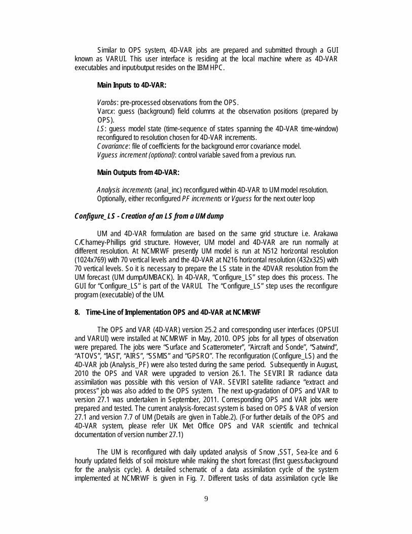
4) User Interface The UIs are X-Windows based and run in the familiar environment of the user's own local workstation (see Fig.1). It is designed to give access to the full functionality of the UM, OPS and VAR whilst speeding up the learning process. Using a central database that works in a distributed environment, the UIs provides an efficient method of defining the runs and managing those definitions. A run definition is known as a job. Users can search for and copy jobs belonging to colleagues, and definitions can even be sent by e-mail from one site to another. This allows colleagues and collaborators at remote sites to increase their efficiency by pooling their effort and knowledge. The job management system also provides help for users wanting to upgrade from one version of the UM/OPS/VAR to another. In addition to the job management system, the UIs contain a comprehensive job definition system. This is an intelligent editor that allows modifications to be made to existing jobs. It is made up of a large number of windows, each with visual cues to ensure that users can quickly see when options have been disabled due to other responses. To further aid the user, all windows have a help button that displays information relating to the options available on the window. Once a job has been defined, the responses are translated into control files that can be read by the UM/OPS/VAR system. On request (with a click of the mouse), the UI will then copy these to the target machine and submit the job. The control files are text based and so a user can easily over-ride the UI by editing the control files. This facilitates the prototyping of new features.

5) Remote access Both the installation scripts and the User Interface will require automatic, unverified, access from the local machine to the remote machine (HPC). In order to facilitate this ssh keys or a .rhosts file need to be set up first.

4. Implementation Process at NCMRWF

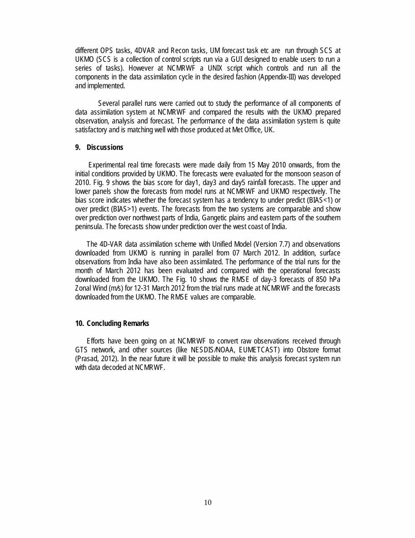
The work on the implementation of UM started in early 2009. A Linux workstation was identified to set up UM repositories. Subversion Code Management system was first installed in the workstation and then configured in server mode. Next Tcl/Tk version 8.4.19 was installed. In order to facilitate unverified access (password less) from the local machine to the remote machine and vice-versa, secure shell (ssh) keys were set up on both machines. In 2009 the remote machine was IBM-P5 based Param Padma and from 2010 onwards the remote machine became IBM-P6 system. Subsequently, repositories of OPS, VAR etc. were set up on the same Linux workstation. The currently available subversion repositories on the server are shown in Fig. 2. The subversion repositories of UM, OPS and VAR at NCMRWF are referred to with the following URLs:

svn://UMRS/UM_repos/UM svn://UMRS/OPS_repos/OPS svn://UMRS/VAR_repos/VAR

At NCMRWF the internal IP address of UM Repository Server (UMRS) is 192.168.0.209.

5

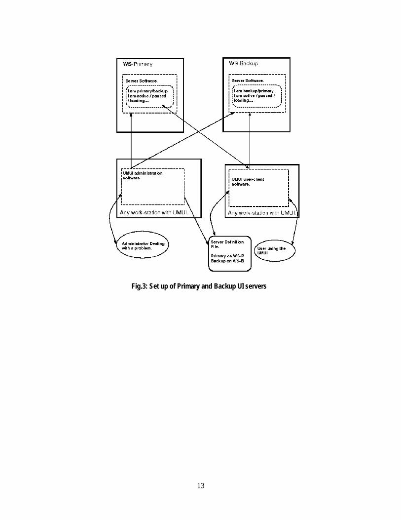
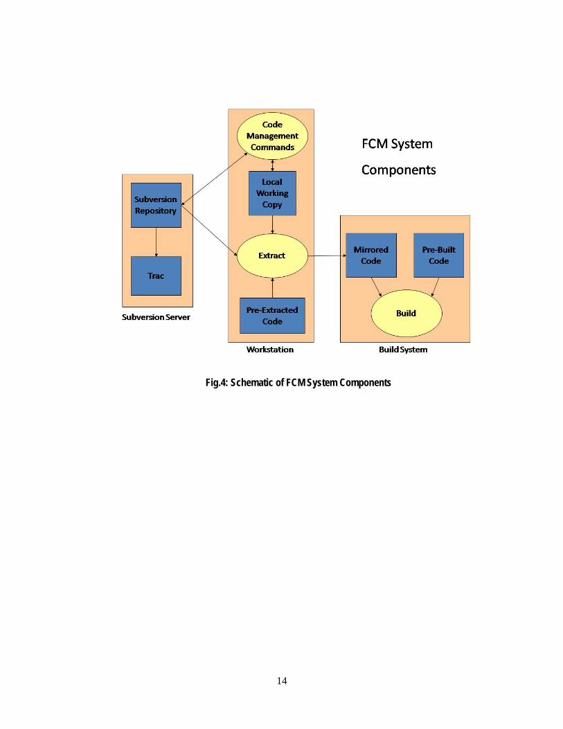
The User Interface’s of UM, OPS and VAR were also setup on the same workstation. Subsequently, a backup server for User Interface (UI) was also set up (Fig. 3). In order to the access the UIs from user desktops (Linux), user client software of the UIs were installed separately in each of them. On many of the desktops subversion and Tcl/Tk had to be installed. In practice the UIs are used to extract the codes from the particular repository to the local machine and then it is mirrored across to the remote (build) system for compilation & execution (Fig. 4).

The initial work of UM implementation started with UM (version 7.1) in early 2009 with

Param Padma (IBM-p5 HPC) and the model code was compiled successfully. However, due to some compiler issues model could not be run successfully. Later with the arrival of IBM-P6 HPC in April 2010, UM (version 7.4) was successfully compiled and tested at N320L50 (~40 km at mid-latitudes) using Met Office Initial conditions. Daily runs of UM7.4 at N320L50 started in June 2010 with Met Office initial conditions. At the end of the monsoon season of 2010, model’s vertical levels were increased to 70. Later on in the same year, model’s horizontal resolution was upgraded to N512 (~25 km at mid-latitudes). During last one year the model’s versions were upgraded to versions 7.5, 7.6, 7.7, 7.8 and 7.9 at repository level. Daily runs with UM version 7.6 started in June 2011 at N512L70 resolution.

The computing time (Wall Clock Time) required to complete a 24 hr forecast with UM at

N512L70 on 16 nodes (16x32) of IBM-p6 HPC in dedicated mode is about 700 sec (~12 minutes). OPS and VAR together takes about 1 hour 15 minutes per cycle of analysis on 16 nodes of IBM-p6 HPC.

6

5. Description of the Unified Model A detailed description of the various components of the Unified Model are given in

Appendix-I. The guidelines for building the UM is provided with the release of each version of the model in “UM Documentation Paper No.X4”. The guidelines for running the UM is provided in “UM Documentation Paper No. X0” made available with each release. The typical procedures involved in UM version upgradation to version 7.7 at NCMRWF are given in Appendix-II.

Regional configurations of UM have also been set up at resolutions 12 km, 4 km and 1.5 km. South Asian Model (SAM) with a resolution of 12 km and 70 vertical levels cover the entire South Asia (approximately 30-115E, 9S-45N). Meso-scale Atmospheric Model (MAM) with a resolution of 4 km and Variable-grid Atmospheric Model (VAM) with a variable grid resolution of 1.5 km and 70 vertical levels have also been set up over Delhi domain approximately covering (76-79E, 26-29N). The rotated latitude-longitude grid used in these configurations provides nearly uniform resolutions over most part of the limited area domains. SAM is run for 3 days and meso-scale configurations are run for even shorter periods mainly for now-casting applications.

The output produced by the UM model is in a format called ‘Fields File’ (FF), which can be readily visualized using ‘xconv’ (Software for file manipulation/conversion) software or can be converted into ‘grads’ or ‘netcdf’ binary formats. Another option is to convert it into PP format which is a special one used at Met Office. Proprietary software IDL (Interactive Data Language) can be used for interactive processing and visualization of UM outputs. At UK Met Office, PV-WAVE library is adapted for IDL with a large collection of routines to support the analysis and visualization of PP format files. At NCMRWF, the UM format is converted to ‘grads’ binary files for primary visualization of operational forecasts. A utility script called “ff2grads.sh” was created using the freely available ‘convsh’ software for the conversion.

6. Description of the Observation Processing System Data assimilation system requires quality controlled observations in suitable format. OPS reads in the observations either from the data base (MetDB, ECMWF ODB etc), BUFR files or from the archived files known as “obstore”. OPS also reads in the model background files (first guess) from the short forecast of UM and prepare the “background observation”. OPS system has different components to carryout various tasks. The “extract and process” component of the OPS is used for observation processing. The task “extract” basically retrieves the observations (all observations including radiance) from the database/file (obstore) and the task “process” then performs the quality control, thinning and then reformats them ready for use in data assimilation. OPS “extract and process” task reformats the input data into various data structures. The three main data structures that are generated to store observation and model data are (a) ob-type structure (b) cx-type structure (c) Model ob-type structure.

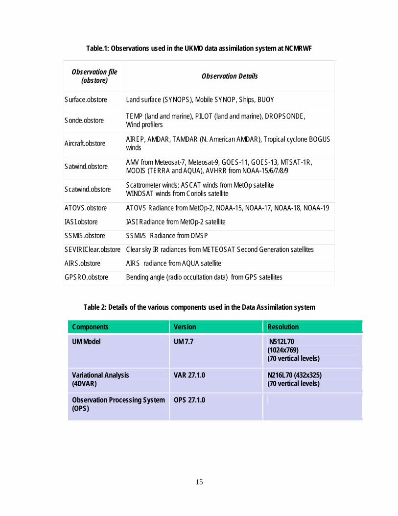
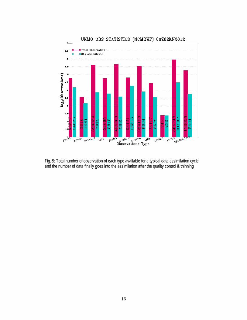
At NCMRWF “obstore” files are the observation input. Each observation type is available in a separate obstore file (namely, Surface.obstore, Scatwind.obstore, Aircraft.obstore, Sonde.obstore, Satwind.obstore, ATOVS.obstore, IASI.obstore, AIRS.obstore, SSMIS.obstore, GPSRO.obstore and SEVIRIClear.obstore) The details of the observations available in each obstore is given in Table.1. Total number of observation of each type available for a typical data assimilation cycle and the number of data finally goes into the

7

assimilation after the quality control and thinning of that cycle is given in Fig.5. OPS carries out conversion of observed quantities (if required), to do quality control of the observation. In some instances this conversion may require significant amounts of processing as in the case with satellite radiance data where a 1D-VAR retrieval is carried out. OPS also apply corrections, if required, to the observational data. Quality control of the observations includes internal consistency check, checks against model background and checks against near neighboring observations. The processed observations are written in files known as “varobs”, corresponding to each observation type. The background (first guess) processing is also a part of the OPS “extract and process”. The observation processing is targeted at a particular UM configuration. Thus the processing for alternate configurations (domain, resolution etc) is completely different. When background field (first guess) processing is done in “extract and process” along with the observation processing, resulting columns of model data are interpolated to the observation location and are passed to the data assimilation system as “varcx” files.

Prior statistics relating to the observations such as details of the observing system,

observations errors, initial probability of gross error, satellite information, fast radiative model coefficients (RTTOV coefficients), satellite biases etc. are being provided to the OPS system. Some of these statistics are updated at regular intervals. OPS also generate a “background error” using the “Background Error Create” component before processing any observation, since the “background error” is an input for the “Extract and Process” step. These geographical varying model errors are determined using model tendency, model gradient and background wind speed information taken from the background (first guess) file.

The OPS software is written in F90 and is designed to be portable across different platforms. At NCMRWF, the OPS system is installed on the IBM HPC (Fig.6). The user interface of the OPS, known as OPSUI, resides in the local machine in a client-server configuration whereas the computational code (OPS executables) resides on the IBM HPC. All OPS jobs are created and processed in the local machine using OPSUI. These jobs are then submitted to the IBM HPC.

Main Inputs to OPS: Observations: Respective obstore file (all observations including radiance) Model background: Three hourly model forecast fields over the assimilation cycle Background error: Prepared by OPS system based on model forecast (background) and the previous cycle’s background error file Fixed files: RTTOV coefficients, SatRad coefficients, SatRad biases, Station list, Sonde coefficient etc.

Main Outputs from OPS:

Varobs: pre-processed observations (“extract and process” output) Varcx: guess model columns at the observation positions (“extract and process” output) Background error: Prepared by “background error create” of OPS system based on model forecast (background) and the previous cycle’s background error file

8

7. Description of the 4D-VAR System

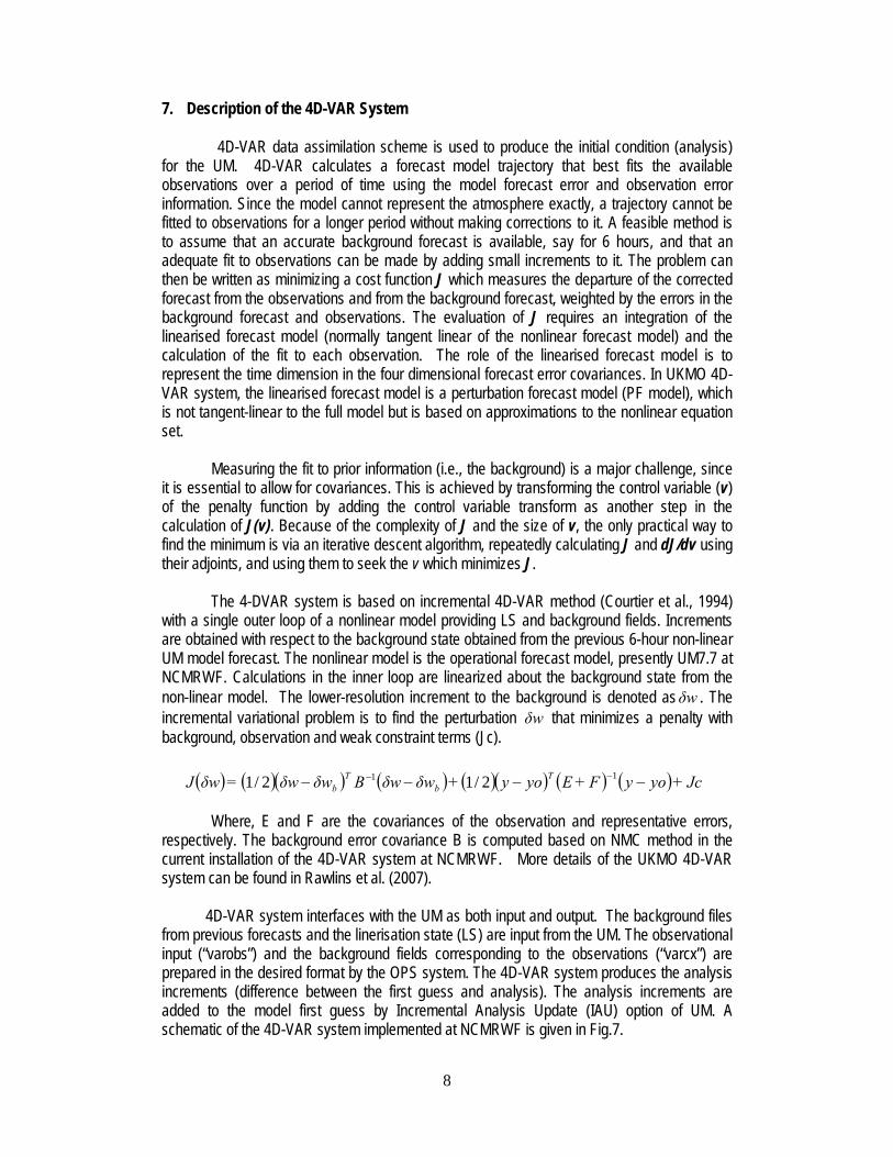
4D-VAR data assimilation scheme is used to produce the initial condition (analysis) for the UM. 4D-VAR calculates a forecast model trajectory that best fits the available observations over a period of time using the model forecast error and observation error information. Since the model cannot represent the atmosphere exactly, a trajectory cannot be fitted to observations for a longer period without making corrections to it. A feasible method is to assume that an accurate background forecast is available, say for 6 hours, and that an adequate fit to observations can be made by adding small increments to it. The problem can then be written as minimizing a cost function J which measures the departure of the corrected forecast from the observations and from the background forecast, weighted by the errors in the background forecast and observations. The evaluation of J requires an integration of the linearised forecast model (normally tangent linear of the nonlinear forecast model) and the calculation of the fit to each observation. The role of the linearised forecast model is to represent the time dimension in the four dimensional forecast error covariances. In UKMO 4D-VAR system, the linearised forecast model is a perturbation forecast model (PF model), which is not tangent-linear to the full model but is based on approximations to the nonlinear equation set.

Measuring the fit to prior information (i.e., the background) is a major challenge, since it is essential to allow for covariances. This is achieved by transforming the control variable (v) of the penalty function by adding the control variable transform as another step in the calculation of J(v). Because of the complexity of J and the size of v, the only practical way to find the minimum is via an iterative descent algorithm, repeatedly calculating J and dJ/dv using their adjoints, and using them to seek the v which minimizes J. The 4-DVAR system is based on incremental 4D-VAR method (Courtier et al., 1994) with a single outer loop of a nonlinear model providing LS and background fields. Increments are obtained with respect to the background state obtained from the previous 6-hour non-linear UM model forecast. The nonlinear model is the operational forecast model, presently UM7.7 at NCMRWF. Calculations in the inner loop are linearized about the background state from the non-linear model. The lower-resolution increment to the background is denoted as δw . The incremental variational problem is to find the perturbation δw that minimizes a penalty with background, observation and weak constraint terms (Jc).

( ) ( )( ) ( ) ( )( ) ( ) ( ) Jc+yoyF+Eyoy+δwδwBδwδw=δwJ Tb

Tb −−−− −− 11 2/12/1

Where, E and F are the covariances of the observation and representative errors, respectively. The background error covariance B is computed based on NMC method in the current installation of the 4D-VAR system at NCMRWF. More details of the UKMO 4D-VAR system can be found in Rawlins et al. (2007). 4D-VAR system interfaces with the UM as both input and output. The background files from previous forecasts and the linerisation state (LS) are input from the UM. The observational input (“varobs”) and the background fields corresponding to the observations (“varcx”) are prepared in the desired format by the OPS system. The 4D-VAR system produces the analysis increments (difference between the first guess and analysis). The analysis increments are added to the model first guess by Incremental Analysis Update (IAU) option of UM. A schematic of the 4D-VAR system implemented at NCMRWF is given in Fig.7.

9

Similar to OPS system, 4D-VAR jobs are prepared and submitted through a GUI known as VARUI. This user interface is residing at the local machine where as 4D-VAR executables and input/output resides on the IBM HPC.

Main Inputs to 4D-VAR: Varobs: pre-processed observations from the OPS. Varcx: guess (background) field columns at the observation positions (prepared by OPS). LS: guess model state (time-sequence of states spanning the 4D-VAR time-window) reconfigured to resolution chosen for 4D-VAR increments. Covariance: file of coefficients for the background error covariance model. Vguess increment (optional): control variable saved from a previous run. Main Outputs from 4D-VAR: Analysis increments (anal_inc) reconfigured within 4D-VAR to UM model resolution. Optionally, either reconfigured PF increments or Vguess for the next outer loop

Configure_LS - Creation of an LS from a UM dump

UM and 4D-VAR formulation are based on the same grid structure i.e. Arakawa C/Charney-Phillips grid structure. However, UM model and 4D-VAR are run normally at different resolution. At NCMRWF presently UM model is run at N512 horizontal resolution (1024x769) with 70 vertical levels and the 4D-VAR at N216 horizontal resolution (432x325) with 70 vertical levels. So it is necessary to prepare the LS state in the 4DVAR resolution from the UM forecast (UM dump/UMBACK). In 4D-VAR, “Configure_LS” step does this process. The GUI for “Configure_LS” is part of the VARUI. The “Configure_LS” step uses the reconfigure program (executable) of the UM. 8. Time-Line of Implementation OPS and 4D-VAR at NCMRWF The OPS and VAR (4D-VAR) version 25.2 and corresponding user interfaces (OPSUI and VARUI) were installed at NCMRWF in May, 2010. OPS jobs for all types of observation were prepared. The jobs were “Surface and Scatterometer”, “Aircraft and Sonde”, “Satwind”, “ATOVS”, “IASI”, “AIRS”, “SSMIS” and “GPSRO”. The reconfiguration (Configure_LS) and the 4D-VAR job (Analysis_PF) were also tested during the same period. Subsequently in August, 2010 the OPS and VAR were upgraded to version 26.1. The SEVIRI IR radiance data assimilation was possible with this version of VAR. SEVIRI satellite radiance “extract and process” job was also added to the OPS system. The next up-gradation of OPS and VAR to version 27.1 was undertaken in September, 2011. Corresponding OPS and VAR jobs were prepared and tested. The current analysis-forecast system is based on OPS & VAR of version 27.1 and version 7.7 of UM (Details are given in Table.2). (For further details of the OPS and 4D-VAR system, please refer UK Met Office OPS and VAR scientific and technical documentation of version number 27.1)

The UM is reconfigured with daily updated analysis of Snow ,SST, Sea-Ice and 6 hourly updated fields of soil moisture while making the short forecast (first guess/background for the analysis cycle). A detailed schematic of a data assimilation cycle of the system implemented at NCMRWF is given in Fig. 7. Different tasks of data assimilation cycle like

10

different OPS tasks, 4DVAR and Recon tasks, UM forecast task etc are run through SCS at UKMO (SCS is a collection of control scripts run via a GUI designed to enable users to run a series of tasks). However at NCMRWF a UNIX script which controls and run all the components in the data assimilation cycle in the desired fashion (Appendix-III) was developed and implemented. Several parallel runs were carried out to study the performance of all components of data assimilation system at NCMRWF and compared the results with the UKMO prepared observation, analysis and forecast. The performance of the data assimilation system is quite satisfactory and is matching well with those produced at Met Office, UK. 9. Discussions

Experimental real time forecasts were made daily from 15 May 2010 onwards, from the initial conditions provided by UKMO. The forecasts were evaluated for the monsoon season of 2010. Fig. 9 shows the bias score for day1, day3 and day5 rainfall forecasts. The upper and lower panels show the forecasts from model runs at NCMRWF and UKMO respectively. The bias score indicates whether the forecast system has a tendency to under predict (BIAS<1) or over predict (BIAS>1) events. The forecasts from the two systems are comparable and show over prediction over northwest parts of India, Gangetic plains and eastern parts of the southern peninsula. The forecasts show under prediction over the west coast of India.

The 4D-VAR data assimilation scheme with Unified Model (Version 7.7) and observations

downloaded from UKMO is running in parallel from 07 March 2012. In addition, surface observations from India have also been assimilated. The performance of the trial runs for the month of March 2012 has been evaluated and compared with the operational forecasts downloaded from the UKMO. The Fig. 10 shows the RMSE of day-3 forecasts of 850 hPa Zonal Wind (m/s) for 12-31 March 2012 from the trial runs made at NCMRWF and the forecasts downloaded from the UKMO. The RMSE values are comparable.

10. Concluding Remarks

Efforts have been going on at NCMRWF to convert raw observations received through GTS network, and other sources (like NESDIS/NOAA, EUMETCAST) into Obstore format (Prasad, 2012). In the near future it will be possible to make this analysis forecast system run with data decoded at NCMRWF.

11

Fig. 1: The main navigation window of the UMUI. Nodes in the tree (left) may be expanded and collapsed. In this example, the atmospheric model node is expanded. Selected nodes are opened up to display windows (right).

12

Fig.2: Currently available subversion repositories on the server

13

Fig.3: Set up of Primary and Backup UI servers

14

Fig.4: Schematic of FCM System Components

15

Table.1: Observations used in the UKMO data assimilation system at NCMRWF

Table 2: Details of the various components used in the Data Assimilation system Components Version Resolution

UM Model UM 7.7 N512L70 (1024x769) (70 vertical levels)

Variational Analysis (4DVAR)

VAR 27.1.0 N216L70 (432x325) (70 vertical levels)

Observation Processing System (OPS)

OPS 27.1.0

Observation file (obstore) Observation Details

Surface.obstore Land surface (SYNOPS), Mobile SYNOP, Ships, BUOY

Sonde.obstore TEMP (land and marine), PILOT (land and marine), DROPSONDE, Wind profilers

Aircraft.obstore AIREP, AMDAR, TAMDAR (N. American AMDAR), Tropical cyclone BOGUS winds

Satwind.obstore AMV from Meteosat-7, Meteosat-9, GOES-11, GOES-13, MTSAT-1R, MODIS (TERRA and AQUA), AVHRR from NOAA-15/6/7/8/9

Scatwind.obstore Scattrometer winds: ASCAT winds from MetOp satellite WINDSAT winds from Coriolis satellite

ATOVS.obstore ATOVS Radiance from MetOp-2, NOAA-15, NOAA-17, NOAA-18, NOAA-19

IASI.obstore IASI Radiance from MetOp-2 satellite

SSMIS.obstore SSMI/S Radiance from DMSP

SEVIRIClear.obstore Clear sky IR radiances from METEOSAT Second Generation satellites

AIRS.obstore AIRS radiance from AQUA satellite

GPSRO.obstore Bending angle (radio occultation data) from GPS satellites

16

Fig. 5: Total number of observation of each type available for a typical data assimilation cycle and the number of data finally goes into the assimilation after the quality control & thinning

17

Fig. 6: Input and Outputs of OPS system (extract and process)

OPS 4DVAR UM

Configure LS

varobs files

varcx files anal_inc

LS files

Umback files

OPS

Observations (obstore)

4DVAR

Modelbackground

Background Error

varcx varobs

Fig. 7: Schematic of 4D-VAR system

18

4DVAR

OPS (Create Background

error)

Background error

Observation (obstore files)

qwqg (cycle-1) .pp_006

OPS (extract & Process)

qwqg (cycle).var_cx

qwqg (cycle).varobs

LS_N108 LS_N216

anal_inc

UM

6 hr forecast file (_da003)

UMBACK (*_ca006 to *_ca011)

Configure_LS

Input_da003

Climatology/fixed files

Fig.8: Schematic of one cycle of UKMO Data Assimilation System implemented at NCMRWF

19

Fig. 9: Bias score for day1, day3 and day5 rainfall forecasts. The upper and lower panels show the forecasts from model runs at NCMRWF and UKMO respectively.

20

Fig. 10: RMSE of day-3 forecasts of 850 hPa Zonal Wind (m/s) for 12-31 March 2012 (a) from the trial runs made at NCMRWF and (b) the forecasts downloaded from the UKMO

21

Appendix-I Description of the Unified Model

1. Overview

The Unified Model (UM) is the name given to the suite of atmospheric and oceanic numerical modelling software developed and used at the Met Office, UK. The formulation of the model supports global and regional domains and is applicable to a wide range of temporal and spatial scales that allow it to be used for both numerical weather prediction and climate modelling as well as a variety of related research activities. The Unified Model was introduced into operational service in 1991. Since then, both its formulation and capabilities have been substantially enhanced.

The modelling system is designed so that it can be run in atmosphere-only, ocean-only or coupled mode. A number of sub-models are also available which may be used in place of or in addition to the main models. These include a simplified model of the ocean, known as the slab model, and models to simulate the thermodynamic and dynamic motion of sea ice. A typical run of the system consists of an optional period of data assimilation followed by a prediction phase. Forecasts from a few hours to a few days ahead are required for numerical weather prediction, while for seasonal forecasting the prediction phase may be few months and while for climate modelling the prediction phase may be for tens, hundreds or even thousands of years. The choice of horizontal and vertical resolution is arbitrary and may be varied by the user. In practice, the resolution is constrained by the available computing power and a number of standard resolutions tend to be used. A separate reconfiguration module allows atmosphere model data to be optionally interpolated to a new grid or area prior to the start of a run.

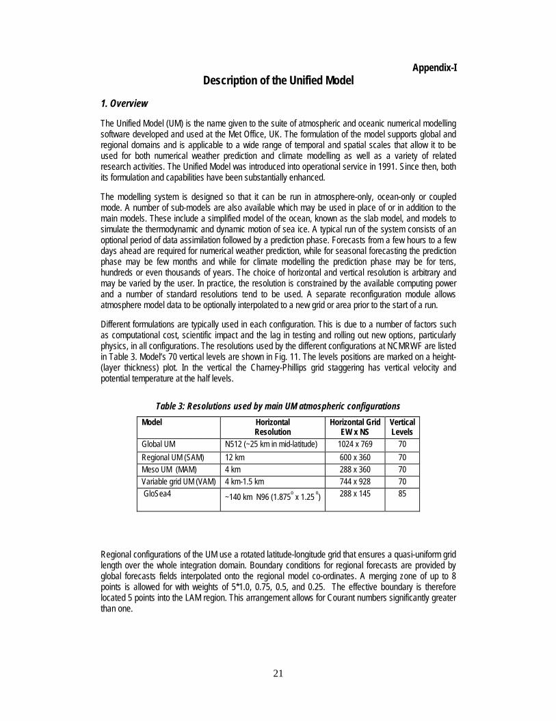
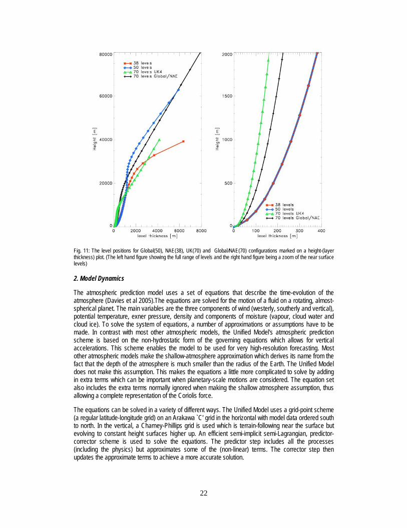
Different formulations are typically used in each configuration. This is due to a number of factors such as computational cost, scientific impact and the lag in testing and rolling out new options, particularly physics, in all configurations. The resolutions used by the different configurations at NCMRWF are listed in Table 3. Model’s 70 vertical levels are shown in Fig. 11. The levels positions are marked on a height-(layer thickness) plot. In the vertical the Charney-Phillips grid staggering has vertical velocity and potential temperature at the half levels.

Table 3: Resolutions used by main UM atmospheric configurations Model Horizontal

Resolution Horizontal Grid

EW x NS Vertical Levels

Global UM N512 (~25 km in mid-latitude) 1024 x 769 70 Regional UM (SAM) 12 km 600 x 360 70 Meso UM (MAM) 4 km 288 x 360 70 Variable grid UM (VAM) 4 km-1.5 km 744 x 928 70 GloSea4 ~140 km N96 (1.875o x 1.25 o) 288 x 145 85

Regional configurations of the UM use a rotated latitude-longitude grid that ensures a quasi-uniform grid length over the whole integration domain. Boundary conditions for regional forecasts are provided by global forecasts fields interpolated onto the regional model co-ordinates. A merging zone of up to 8 points is allowed for with weights of 5*1.0, 0.75, 0.5, and 0.25. The effective boundary is therefore located 5 points into the LAM region. This arrangement allows for Courant numbers significantly greater than one.

22

Fig. 11: The level positions for Global(50), NAE(38), UK(70) and Global/NAE(70) configurations marked on a height-(layer thickness) plot. (The left hand figure showing the full range of levels and the right hand figure being a zoom of the near surface levels)

2. Model Dynamics

The atmospheric prediction model uses a set of equations that describe the time-evolution of the atmosphere (Davies et al 2005).The equations are solved for the motion of a fluid on a rotating, almost-spherical planet. The main variables are the three components of wind (westerly, southerly and vertical), potential temperature, exner pressure, density and components of moisture (vapour, cloud water and cloud ice). To solve the system of equations, a number of approximations or assumptions have to be made. In contrast with most other atmospheric models, the Unified Model's atmospheric prediction scheme is based on the non-hydrostatic form of the governing equations which allows for vertical accelerations. This scheme enables the model to be used for very high-resolution forecasting. Most other atmospheric models make the shallow-atmosphere approximation which derives its name from the fact that the depth of the atmosphere is much smaller than the radius of the Earth. The Unified Model does not make this assumption. This makes the equations a little more complicated to solve by adding in extra terms which can be important when planetary-scale motions are considered. The equation set also includes the extra terms normally ignored when making the shallow atmosphere assumption, thus allowing a complete representation of the Coriolis force.

The equations can be solved in a variety of different ways. The Unified Model uses a grid-point scheme (a regular latitude-longitude grid) on an Arakawa `C' grid in the horizontal with model data ordered south to north. In the vertical, a Charney-Phillips grid is used which is terrain-following near the surface but evolving to constant height surfaces higher up. An efficient semi-implicit semi-Lagrangian, predictor-corrector scheme is used to solve the equations. The predictor step includes all the processes (including the physics) but approximates some of the (non-linear) terms. The corrector step then updates the approximate terms to achieve a more accurate solution.

23

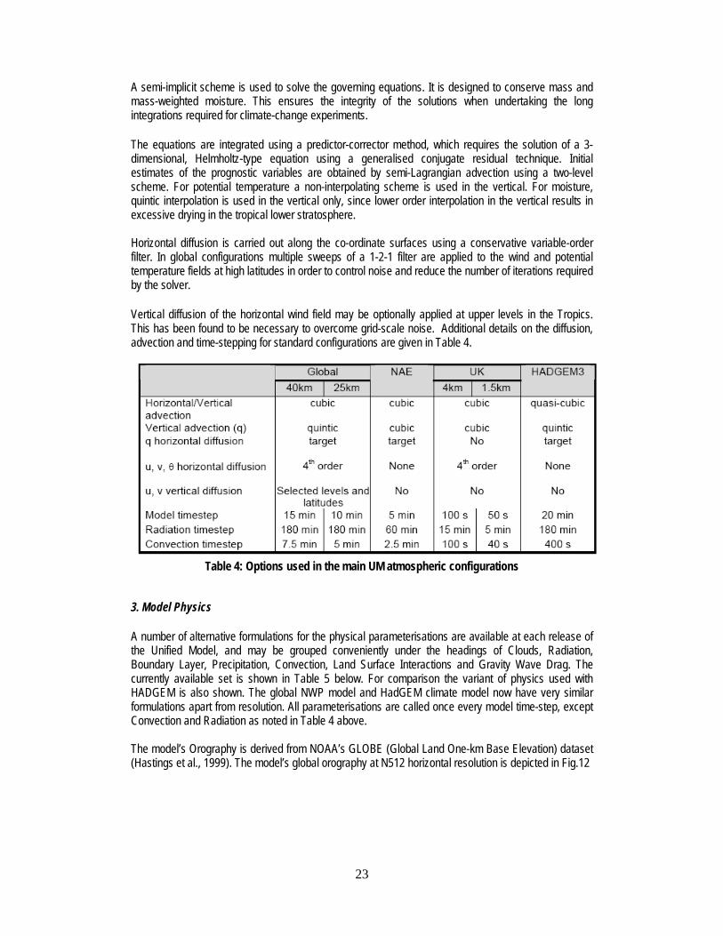
A semi-implicit scheme is used to solve the governing equations. It is designed to conserve mass and mass-weighted moisture. This ensures the integrity of the solutions when undertaking the long integrations required for climate-change experiments. The equations are integrated using a predictor-corrector method, which requires the solution of a 3-dimensional, Helmholtz-type equation using a generalised conjugate residual technique. Initial estimates of the prognostic variables are obtained by semi-Lagrangian advection using a two-level scheme. For potential temperature a non-interpolating scheme is used in the vertical. For moisture, quintic interpolation is used in the vertical only, since lower order interpolation in the vertical results in excessive drying in the tropical lower stratosphere. Horizontal diffusion is carried out along the co-ordinate surfaces using a conservative variable-order filter. In global configurations multiple sweeps of a 1-2-1 filter are applied to the wind and potential temperature fields at high latitudes in order to control noise and reduce the number of iterations required by the solver. Vertical diffusion of the horizontal wind field may be optionally applied at upper levels in the Tropics. This has been found to be necessary to overcome grid-scale noise. Additional details on the diffusion, advection and time-stepping for standard configurations are given in Table 4.

Table 4: Options used in the main UM atmospheric configurations

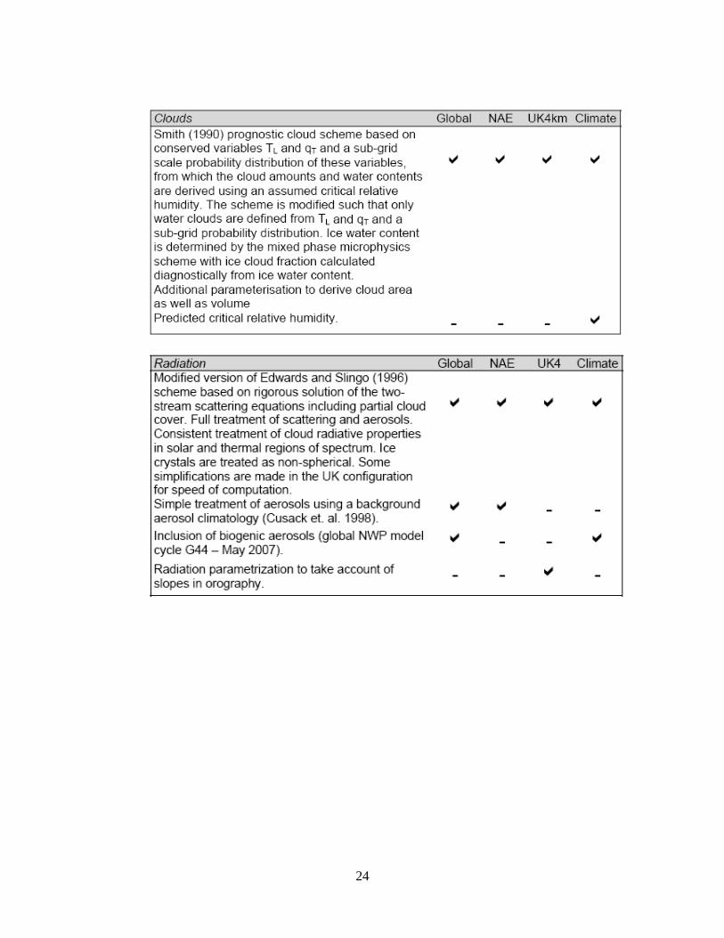
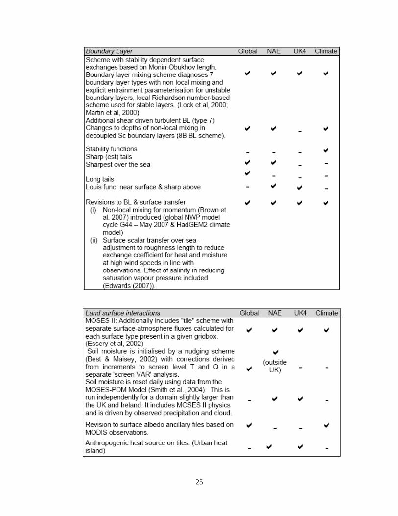
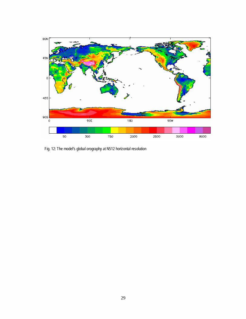
3. Model Physics A number of alternative formulations for the physical parameterisations are available at each release of the Unified Model, and may be grouped conveniently under the headings of Clouds, Radiation, Boundary Layer, Precipitation, Convection, Land Surface Interactions and Gravity Wave Drag. The currently available set is shown in Table 5 below. For comparison the variant of physics used with HADGEM is also shown. The global NWP model and HadGEM climate model now have very similar formulations apart from resolution. All parameterisations are called once every model time-step, except Convection and Radiation as noted in Table 4 above. The model’s Orography is derived from NOAA’s GLOBE (Global Land One-km Base Elevation) dataset (Hastings et al., 1999). The model’s global orography at N512 horizontal resolution is depicted in Fig.12

24

25

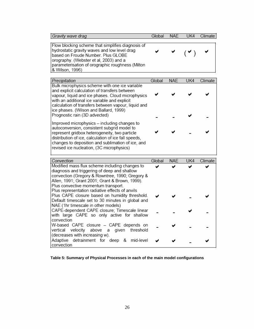
26

Table 5: Summary of Physical Processes in each of the main model configurations

27

Reconfiguration

The reconfiguration stage processes the model's initial data. For the atmosphere mode, it allows the horizontal or vertical resolution of the data to be changed or the creation of a limited area region. Ancillary data may also be incorporated into the initial data. Fields such as the specification of the height of orography or the land-sea mask, for example, may be overwritten by more appropriate values if the horizontal resolution has been changed. Other facilities available within the reconfiguration include the ability to incorporate ensemble perturbations, tracer fields and the transplanting of prognostic data.

Tracers

The atmospheric component supports the advection of passive tracers using a semi-Lagrangian advection scheme. This facility may be used to examine dispersion from point sources or as the basis for more involved chemical modelling by the addition of extra code. For example, atmospheric forecast configurations of the model include an aerosol variable which is advected using the tracer scheme, and may optionally have sources and sinks applied. This is used to estimate visibility, and may be adjusted by the assimilation of visibility data. For the ocean model, tracers provide a useful means of examining the model's representation of physical, dynamical, chemical and biological processes. A range of numerical schemes is available to enable advection both horizontally and vertically.

Ancillary Data

New ancillary data may be incorporated as integration proceeds to allow for the effects of temporally varying quantities such as surface vegetation, snow cover or wind-stress. The choice of whether to include ancillary data will depend on the application. For example, the system supports daily updating of sea-surface temperatures based on climatological or analysed data - but this facility is not needed in ocean-only or coupled ocean-atmosphere runs of the model. In fact options exist to allow most boundary forcing variables to be predicted. However, it is often necessary to constrain such fields to observed or climatological values for reasons of computational economy or scientific expediency.

OASIS Coupler

The aim of the OASIS (Ocean Atmosphere Sea Ice Soil) coupler, developed at the European Centre for Research and Advanced Training in Scientific Computation (CERFACS), is to provide a tool for coupling independent GCMs of atmosphere and ocean as well as other climate modules. It is possible for the models to run on different platforms. Work is in progress to enable the Atmosphere, Ocean (NEMO) and Sea-Ice (CICE) sub-models to be coupled via the OASIS3 and OASIS4 couplers from UM version 7.0.

Diagnostic Processing

Diagnostic data output from the model may be defined and output on a time-step by time-step basis. Horizontal fields, sub-areas or time series may be requested, along with the accumulation, time meaning or spatial meaning of fields. The output may also be split across a number of files in order to facilitate the separate post-processing of classes of diagnostics. UM Storage handling and diagnostic system (STASH) is to be set up inside the job beforehand itself for this purpose. Initially unit numbers 60, 62 and 64 were set up with minimum parameters for operational forecast visualization. A more detailed list of diagnostics available in UM was prepared in consultation with experts and incorporated later to be written in unit

28

numbers 61 (single level instantaneous fields), 63 (multilevel instantaneous fields) and 65 (time averaged fields).

Output

The results of model integration are stored in a format compatible with other file types used within the Unified Model system. Several utilities exist which will convert them into a format suitable for further processing. These formats include GRIB--the WMO standard for storing fields of meteorological data in a machine independent format. This facility is not yet provided as standard in the ported UM. Utilities to print out and compare the contents of Unified Model files are available. These, coupled with the bit reproducibility facility (see below), offer a powerful development and debugging aid.

Computing Requirements The code was originally written in FORTRAN 77 and from UM version 6.3 onwards FORTRAN 90 is used. A small number of low-level service routines are written in ANSI C to facilitate portability. The model will normally require a powerful supercomputer for time critical production work. It is written to be efficient on distributed memory massively parallel processing (MPP) computers such as the Cray T3E, but will also run on ``clustered" shared memory computers, such as the IBM p690, as well as on a single node of a parallel machine. The code is bit reproducible independently of the number of processing elements used. The code may also be run on workstation systems and desktop PCs running the Linux operating system using the IEEE standard for representing floating point numbers. Workstations and Linux PCs are particularly suited to development work or research activities requiring the use of low resolution configurations of the model.

29

Fig. 12: The model’s global orography at N512 horizontal resolution

30

Appendix-II UM Upgradation to UM7.7

Backup of UM repos cd $HOME/SVN_HOTCOPY UM_repos UM_repos_Aug11 svnadmin hotcopy /home/moum/weather/UM_repos $HOME/SVN_HOTCOPY/UM_repos cd $HOME/SVN_DUMPS backup_UM_repos.svn.gz backup_UM_repos.svn.gz_Aug11 svnadmin dump /home/moum/weather/UM_repos >backup_UM_repos.svn gzip backup_UM_repos.svn cd $HOME/BACKUP_Repos mv UM_repos UM_repos_Aug11 cp -rp $HOME/weather/UM_repos UM_repos ### Start the upgradations process cd /home/moum/um_packages/UM/vn7.7 tar -xzf Patchfiles.tgz cd Patchfiles tar –xzf GCOM_vn3.6-vn3.7_patch.tgz GCOM_vn3.6-vn3.7_patch/fcm-import-patch file:///home/moum/weather/UM_repos/GCOM/trunk Committed revision 477 tar –xzf Admin_vn7.6-vn7.7_patch.tgz Admin_vn7.6-vn7.7_patch/fcm-import-patch file:///home/moum/weather/UM_repos/Admin/trunk Committed revision 483 tar –xzf UM_vn7.6-vn7.7_patch.tgz UM_vn7.6-vn7.7_patch/fcm-import-patch file:///home/moum/weather/UM_repos/UM/trunk Committed revision 600 tar -xzf Exported_DRHOOK_vn1.1.tgz svn import Exported_DRHOOK_vn1.1 file:///home/moum/weather/UM_repos -m 'Initial Import of DRHOOK code' Committed revision 601 fcm branch --create --name ncm_gcom3.7_changes --revision head svn://UMRS/UM_repos/GCOM/trunk Committed revision 602 cd $HOME/UM_vn7.7 fcm co svn://UMRS/UM_repos/GCOM/branches/dev/moum/r477_ncm_gcom3.7_changes GCOM.wc cd GCOM.wc/build/ext_scripts/ fcm copy $HOME/UM_vn7.6/GCOM.wc/build/ext_scripts/ncm_ibmp6.scr ncm_ibmp6.scr replace 7.6 with 7.7 in ncm_ibmp6.scr fcm commit Committed revision 603 cd $HOME/UM_vn7.7/GCOM.wc/build/configs/machines fcm copy /home/moum/UM_vn7.6/GCOM.wc/build/configs/machines/ncm_ibm_pwr6_serial.cfg ncm_ibm_pwr6_serial.cfg fcm copy /home/moum/UM_vn7.6/GCOM.wc/build/configs/machines/ncm_ibm_pwr6_mpp.cfg ncm_ibm_pwr6_mpp.cfg made changes to make them similar to meto_ibm_pwr6*.cfg fcm commit Committed revision 604 To extract GCOM source files to IBM HPC

31

/home/moum/UM_vn7.7/GCOM.wc/build/ext_scripts/ncm_ibmp6.scr ## Do the following on IBM HPC to build & test GCOM cd /gpfs1/home/moum/UM/vn7.7/GCOM/ncm_ibm_pwr6_mpp fcm build cd /gpfs1/home/moum/UM/vn7.7/GCOM/ncm_ibm_pwr6_serial fcm build cd /gpfs1/home/moum/UM/vn7.7/GCOM/ncm_ibm_pwr6_mpp_mpl_test fcm build cd /gpfs1/home/moum/UM/vn7.7/GCOM/ncm_ibm_pwr6_mpp_gcom_test fcm build cd /gpfs1/home/moum/UM/vn7.7/GCOM/ncm_ibm_pwr6_mpp_mpl_test cp -p /gpfs1/home/moum/UM/vn7.6/GCOM/ncm_ibm_pwr6_mpp_mpl_test/poe.sh . cp -p /gpfs1/home/moum/UM/vn7.6/GCOM/ncm_ibm_pwr6_mpp_mpl_test/hostfile_6 . poe.sh cd /gpfs1/home/moum/UM/vn7.7/GCOM/ncm_ibm_pwr6_mpp_gcom_test cp -p /gpfs1/home/moum/UM/vn7.6/GCOM/ncm_ibm_pwr6_mpp_gcom_test/poe.sh . cp -p /gpfs1/home/moum/UM/vn7.6/GCOM/ncm_ibm_pwr6_mpp_gcom_test/hostfile_8 . poe.sh ## Installation of UM Admin fcm branch --create --name ncm_um7.7_admin --revision head svn://UMRS/UM_repos/Admin/trunk Committed revision 605 cd $HOME/UM_vn7.7 fcm co svn://UMRS/UM_repos/Admin/branches/dev/moum/r483_ncm_um7.7_admin Admin.wc cd Admin.wc/Install_scripts/Configs fcm copy $HOME/UM_vn7.6/Admin.wc/Install_scripts/Configs/IBM-pwr6-32-ncm . fcm copy $HOME/UM_vn7.6/Admin.wc/Install_scripts/Configs/IBM-pwr6-ncm . vi IBM-pwr6-ncm --- replace 7.6 with 7.7 vi IBM-pwr6-32-ncm -- replace 7.6 with 7.7 cd /home/moum/UM_vn7.7/Admin.wc/Install_scripts fcm copy UmBuildSmllExecs UmBuildSmllExecs_original vi UmBuildSmllExecs Removed "rdest:remote shell" line from UmBuildSmllExecs fcm commit Committed revision 606 ---->create um_conf file cd /home/moum/UM_vn7.7/Admin.wc/Install_scripts UmSetup -f Configs/IBM-pwr6-ncm *** UM Branch creation etc. ... fcm branch --create --name ncm_UM7.7_branch --revision head svn://UMRS/UM_repos/UM/trunk branch: svn://UMRS/UM_repos/UM/branches/dev/moum/r600_ncm_UM7.7_branch Committed revision 607 cd /home/moum/UM_vn7.7/ fcm co svn://UMRS/UM_repos/UM/branches/dev/moum/r600_ncm_UM7.7_branch UM.wc Checked out revision 607 cd /home/moum/UM_vn7.7/UM.wc/src/configs/machines fcm cp ibm-pwr6-meto ibm-pwr6-ncm

32

++++ => svn copy ibm-pwr6-meto ibm-pwr6-ncm ++++ A ibm-pwr6-ncm cd /home/moum/UM_vn7.7/UM.wc/src/configs/machines/ibm-pwr6-ncm vi machine.cfg --> included gcpp & -berok cd /home/moum/UM_vn7.7/UM.wc/src/configs/machines/ibm-pwr6-ncm/ext_libs vi gcom_mpp.cfg vi gcom_serial.cfg vi netcdf.cfg vi drhook.cfg ==> made changes to path in all above files cd /home/moum/UM_vn7.7/UM.wc/src/configs/bindings vi container.cfg ---> commented out "rdest:remote_shell" line ... fcm commit Committed revision 608 cd /home/moum/UM_vn7.7/UM.wc/src/configs/machines/ibm-pwr6-ncm/ext_libs vi default_paths.cfg ----> Inserted the correct paths & removed path of DRHOOK fcm commit Committed revision 611 cd /home/moum/UM_vn7.7/Admin.wc/Install_scripts UmInstall -f Configs/IBM-pwr6-ncm -v 7.7 UmBuildSmllExecs -r svn://UMRS/UM_repos/UM/branches/dev/moum/r600_ncm_UM7.7_branch -f Configs/IBM-pwr6-ncm -v head --vnpath vn7.7 --envver 7.7 cd /home/moum/UM_vn7.7/Admin.wc/Install_scripts UmBuildSmllExecs -r svn://UMRS/UM_repos/UM/branches/dev/moum/r600_ncm_UM7.7_branch -f Configs/IBM-pwr6-ncm -v head --vnpath vn7.7 --envver 7.7 ---> All small executable builds completed on remote machine Thu Sep 1 14:26:31 2011 ---> All small executable wrapper extractions completed Thu Sep 1 14:27:03 2011. ***************************************************************************** UMUI upgradation ------ cd $HOME/um_packages/UM/vn7.7 tar -zxf umui_package.tgz cd umui_package tar -xzf umui2.0.main.tar.gz cd $HOME/umui_package/umui2.0 cp -rp /home/moum/um_packages/UM/vn7.7/umui_package/umui2.0.main/vn7.7 . cd $HOME/umui_package/umui2.0/updates cp -rp /home/moum/um_packages/UM/vn7.7/umui_package/umui2.0.main/updates/7.6-7.7.tcl . chmod 755 7.6-7.7.tcl cd $HOME/umui_package/umui2.0/vn7.7/processing cp -p nds_bld_gencmd nds_bld_gencmd_original vi nds_bld_gencmd -->comment out 2 lines containing "prg" cd $HOME/umui_package/ghui2.0/apps vi umui.def ---> Introduce line containing "vn7.7"

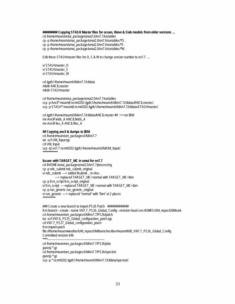
33

######### Copying STASH Master files for ocean, Wave & Slab models from older versions ... cd /home/moum/umui_package/umui2.0/vn7.7/variables cp -p /home/moum/umui_package/umui2.0/vn7.6/variables/*O . cp -p /home/moum/umui_package/umui2.0/vn7.6/variables/*S . cp -p /home/moum/umui_package/umui2.0/vn7.6/variables/*W . Edit these STASHmaster files for O, S & W to change version number to vn7.7 ... vi STASHmaster_O vi STASHmaster_S vi STASHmaster_W cd /gpfs1/home/moum/UM/vn7.7/ctldata mkdir ANCILmaster mkdir STASHmaster cd /home/moum/umui_package/umui2.0/vn7.7/variables scp -p Ancil* moum@ncmr0202:/gpfs1/home/moum/UM/vn7.7/ctldata/ANCILmaster/. scp -p STASH* moum@ncmr0202:/gpfs1/home/moum/UM/vn7.7/ctldata/STASHmaster/. cd /gpfs1/home/moum/UM/vn7.7/ctldata/ANCILmaster ## >>>on IBM mv AncilFields_A ANCILfields_A mv AncilFiles_A ANCILfiles_A ## Copying ancil & dumps to IBM cd /home/moum/um_packages/UM/vn7.7 tar -xzf UM_Input.tgz cd UM_Input scp -rp vn7.7 ncmr0202:/gpfs1/home/moum/UM/UM_Input/. ************* Issues with TARGET_MC in umui for vn7.7 cd $HOME/umui_package/umui2.0/vn7.7/processing cp -p nds_submit nds_submit_original vi nds_submit ---> added llsubmit .. in else.. ---> replaced TARGET_MC=normal with TARGET_MC=ibm cp -p fcm_script fcm_script_original vi fcm_script --- replaced TARGET_MC=normal with TARGET_MC=ibm cp -p run_generic run_generic_original vi run_generic ----> replaced "normal" with "ibm" at 2 places *********** ### Create a new branch to import PS26 Patch ############# fcm branch --create --name VN7.7_PS26_Global_Config --revision head svn://UMRS/UM_repos/UM/trunk cd /home/moum/um_packages/UM/vn7.7/PS26/patch tar -xzf VN7.6_PS25_Global_configuration_patch.tgz cd VN7.7_PS27_Global_configuration_patch fcm-import-patch file:///home/moum/weather/UM_repos/UM/branches/dev/moum/r600_VN7.7_PS26_Global_Config Committed revision 646 ****---------------------------------------------------------- cd /home/moum/um_packages/UM/vn7.7/PS26/jobs gunzip *.gz cd /home/moum/um_packages/UM/vn7.7/PS26/spectral gunzip *.gz scp -p * ncmr0202:/gpfs1/home/moum/UM/vn7.7/ctldata/spectral/.

34

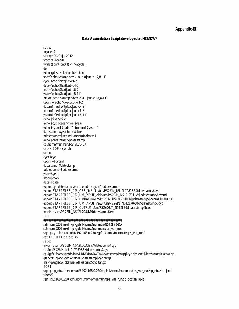
Appendix-III

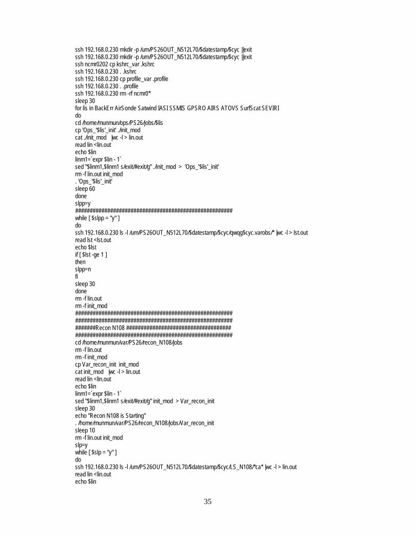
Data Assimilation Script developed at NCMRWF set -x ncycle=4 stamp='00z01jan2012' typeset -i cnt=0 while (( (cnt=cnt+1) <= $ncycle )) do echo 'gdas cycle number ' $cnt fext=ècho $stamp|adv.x -n -a 0|cut -c1-7,8-11` cyc=ècho $fext|cut -c1-2` date=ècho $fext|cut -c4-5` mon=ècho $fext|cut -c6-7` year=ècho $fext|cut -c8-11` pfext=ècho $stamp|adv.x -n -r 1|cut -c1-7,8-11` cycm1=ècho $pfext|cut -c1-2` datem1=ècho $pfext|cut -c4-5` monm1=ècho $pfext|cut -c6-7` yearm1=ècho $pfext|cut -c8-11` echo $fext $pfext echo $cyc $date $mon $year echo $cycm1 $datem1 $monm1 $yearm1 datestamp=$year$mon$date pdatestamp=$yearm1$monm1$datem1 echo $datestamp $pdatestamp cd /home/munmun/N512L70-DA cat << EOF > cyc.sh set -x cyc=$cyc cycm1=$cycm1 datestamp=$datestamp pdatestamp=$pdatestamp year=$year mon=$mon date=$date export cyc datestamp year mon date cycm1 pdatestamp export STARTFILES_DIR_OBS_INPUT=/um/PS26IN_N512L70/OBS/$datestamp/$cyc export STARTFILES_DIR_UM_INPUT_old=/um/PS26IN_N512L70/UM/$pdatestamp/$cycm1 export STARTFILES_DIR_UMBACK=/um/PS26IN_N512L70/UM/$pdatestamp/$cycm1/UMBACK export STARTFILES_DIR_UM_INPUT_new=/um/PS26IN_N512L70/UM/$datestamp/$cyc export STARTFILES_DIR_OUTPUT=/um/PS26OUT_N512L70/$datestamp/$cyc mkdir -p /um/PS26IN_N512L70/UM/$datestamp/$cyc EOF ############################################### ssh ncmr0202 mkdir -p /gpfs1/home/munmun/N512L70-DA ssh ncmr0202 mkdir -p /gpfs1/home/munmun/ops_var_run scp -p cyc.sh [email protected]:/gpfs1/home/munmun/ops_var_run/. cat << EOF1 > cp_obs.sh set -x mkdir -p /um/PS26IN_N512L70/OBS/$datestamp/$cyc cd /um/PS26IN_N512L70/OBS/$datestamp/$cyc cp /gpfs1/home/prod/idata/UKMOInit/DATA/$datestamp/qwqg$cyc.obstore.$datestamp$cyc.tar.gz . gtar -xzf qwqg$cyc.obstore.$datestamp$cyc.tar.gz rm -f qwqg$cyc.obstore.$datestamp$cyc.tar.gz EOF1 scp -p cp_obs.sh [email protected]:/gpfs1/home/munmun/ops_var_run/cp_obs.sh ||exit sleep 5 ssh 192.168.0.230 ksh /gpfs1/home/munmun/ops_var_run/cp_obs.sh ||exit

35

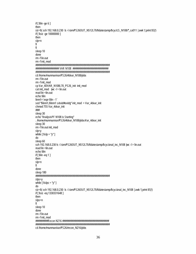
ssh 192.168.0.230 mkdir -p /um/PS26OUT_N512L70/$datestamp/$cyc ||exit ssh 192.168.0.230 mkdir -p /um/PS26OUT_N512L70/$datestamp/$cyc ||exit ssh ncmr0202 cp kshrc_var .kshrc ssh 192.168.0.230 . .kshrc ssh 192.168.0.230 cp profile_var .profile ssh 192.168.0.230 . .profile ssh 192.168.0.230 rm -rf ncmr0* sleep 30 for lis in BackErr AirSonde Satwind IASI SSMIS GPSRO AIRS ATOVS SurfScat SEVIRI do cd /home/munmun/ops/PS26/jobs/$lis cp 'Ops_'$lis'_init' ./init_mod cat ./init_mod |wc -l > lin.out read lin <lin.out echo $lin linm1=èxpr $lin - 1` sed "$linm1,$linm1 s/exit/#exit/g" ./init_mod > 'Ops_'$lis'_init' rm -f lin.out init_mod . 'Ops_'$lis'_init' sleep 60 done slpp=y ###################################################### while [ $slpp = "y" ] do ssh 192.168.0.230 ls -l /um/PS26OUT_N512L70/$datestamp/$cyc/qwqg$cyc.varobs/* |wc -l > lst.out read lst <lst.out echo $lst if [ $lst -ge 1 ] then slpp=n fi sleep 30 done rm -f lin.out rm -f init_mod ###################################################### ###################################################### #######Recon N108 #################################### ###################################################### cd /home/munmun/var/PS26/recon_N108/jobs rm -f lin.out rm -f init_mod cp Var_recon_init init_mod cat init_mod |wc -l > lin.out read lin <lin.out echo $lin linm1=èxpr $lin - 1` sed "$linm1,$linm1 s/exit/#exit/g" init_mod > Var_recon_init sleep 30 echo "Recon N108 is Starting" . /home/munmun/var/PS26/recon_N108/jobs/Var_recon_init sleep 10 rm -f lin.out init_mod slp=y while [ $slp = "y" ] do ssh 192.168.0.230 ls -l /um/PS26OUT_N512L70/$datestamp/$cyc/LS_N108/*ca* |wc -l > lin.out read lin <lin.out echo $lin

36

if [ $lin -ge 6 ] then siz=$( ssh 192.168.0.230 ls -l /um/PS26OUT_N512L70/$datestamp/$cyc/LS_N108/*_ca011 | awk '{ print $5}') if [ $siz -ge 10000000 ] then slp=n fi fi sleep 10 done rm -f lin.out rm -f init_mod ###################################################### ################# VAR N108 ########################## ###################################################### cd /home/munmun/var/PS26/4dvar_N108/jobs rm -f lin.out rm -f init_mod cp Var_4DVAR_N108L70_PS26_init init_mod cat init_mod |wc -l > lin.out read lin <lin.out echo $lin linm1=èxpr $lin - 1` sed "$linm1,$linm1 s/exit/#exit/g" init_mod > Var_4dvar_init chmod 755 Var_4dvar_init ### sleep 30 echo "AnalysisPF N108 is Starting" . /home/munmun/var/PS26/4dvar_N108/jobs/Var_4dvar_init sleep 30 rm -f lin.out init_mod slp=y while [ $slp = "y" ] do sleep 60 ssh 192.168.0.230 ls -l /um/PS26OUT_N512L70/$datestamp/$cyc/anal_inc_N108 |wc -l > lin.out read lin <lin.out echo $lin if [ $lin -eq 1 ] then slp=n fi done sleep 180 ###################################################### slps=y while [ $slps = "y" ] do siz=$( ssh 192.168.0.230 ls -l /um/PS26OUT_N512L70/$datestamp/$cyc/anal_inc_N108 | awk '{ print $5}') if [ $siz -eq 1330331648 ] then slps=n fi sleep 10 done rm -f lin.out rm -f init_mod #########Recon N216 ################################## ###################################################### cd /home/munmun/var/PS26/recon_N216/jobs

37

rm -f lin.out rm -f init_mod cp Var_recon_init init_mod cat init_mod |wc -l > lin.out read lin <lin.out echo $lin linm1=èxpr $lin - 1` sed "$linm1,$linm1 s/exit/#exit/g" init_mod > Var_recon_init sleep 30 echo "Recon N216 is Starting" . /home/munmun/var/PS26/recon_N216/jobs/Var_recon_init sleep 10 rm -f lin.out init_mod slp=y while [ $slp = "y" ] do ssh 192.168.0.230 ls -l /um/PS26OUT_N512L70/$datestamp/$cyc/LS/*ca* |wc -l > lin.out read lin <lin.out echo $lin if [ $lin -ge 6 ] then siz=$( ssh 192.168.0.230 ls -l /um/PS26OUT_N512L70/$datestamp/$cyc/LS/*_ca011 | awk '{ print $5}') if [ $siz -eq 443678720 ] then slp=n fi fi sleep 10 done rm -f lin.out rm -f init_mod ##################################################### ############## VAR N216 ############################# ##################################################### cd /home/munmun/var/PS26/4dvar_N216/jobs rm -f lin.out rm -f init_mod cp Var_4DVAR_N216L70_PS26_init init_mod cat init_mod |wc -l > lin.out read lin <lin.out echo $lin linm1=èxpr $lin - 1` sed "$linm1,$linm1 s/exit/#exit/g" init_mod > Var_4dvar_init chmod 755 /home/munmun/var/PS26/4dvar_N216/jobs/* echo "AnalysisPF N216 is Starting" . /home/munmun/var/PS26/4dvar_N216/jobs/Var_4dvar_init sleep 30 rm -f lin.out init_mod slp=y while [ $slp = "y" ] do sleep 60 ssh 192.168.0.230 ls -l /um/PS26OUT_N512L70/$datestamp/$cyc/anal_inc |wc -l > lin.out read lin <lin.out echo $lin if [ $lin -eq 1 ] then slp=n fi done

38

sleep 180 #################### slps=y while [ $slps = "y" ] do siz=$( ssh 192.168.0.230 ls -l /um/PS26OUT_N512L70/$datestamp/$cyc/anal_inc | awk '{ print $5}') if [ $siz -eq 1330331648 ] then slps=n fi sleep 10 done ###################################################### ###################################################### ###################################################### ###################################################### ##Observation Statistics Preperation cat << EOF6 > ncmr_stat.sh ksh /um/ncmr_obs/stat/ops-stat.sh $cyc $datestamp ksh /um/ncmr_obs/stat/plot.sh $stamp $cyc $date $mon $year EOF6 scp -p ncmr_stat.sh [email protected]:/gpfs1/home/munmun/ops_var_run/. ||exit ssh 192.168.0.230 ksh /gpfs1/home/munmun/ops_var_run/ncmr_stat.sh ||exit ###################################################### ###################################################### ###################################################### ################################################## if [ $cyc -eq 00 ] then cycm6=06 fi if [ $cyc -eq 06 ] then cycm6=12 fi if [ $cyc -eq 12 ] then cycm6=18 fi if [ $cyc -eq 18 ] then cycm6=00 fi ###################################################### cd /home/munmun/N512L70-DA cat << EOF2 > cp_surf.sh set -x mkdir -p /um/PS26_SURF/SURF cd /um/PS26_SURF/SURF cp /gpfs1/home/prod/idata/UKMOInit/DATA/$datestamp/qwqu$cyc.$datestamp$cycm6'.smc.gz' .||exit gzip -d qwqu$cyc.$datestamp$cycm6'.smc.gz' cp qwqu$cyc.$datestamp$cycm6'.smc' daily.smc ###################################################### rm -f *.gz EOF2 ###################################################### cat << EOF9 > cp_surf_06.sh set -x mkdir -p /um/PS26_SURF/SURF cd /um/PS26_SURF/SURF

39

cp /gpfs1/home/prod/idata/UKMOInit/DATA/$datestamp/qwgl.daily.$datestamp'12.sst.gz' .||exit cp /gpfs1/home/prod/idata/UKMOInit/DATA/$datestamp/qwgl.daily.$datestamp'12.ice.gz' .||exit gzip -d qwgl.daily.$datestamp'12.sst.gz' gzip -d qwgl.daily.$datestamp'12.ice.gz' mv ./qwgl.daily.$datestamp'12.sst' ./daily.sst mv ./qwgl.daily.$datestamp'12.ice' ./daily.seaice cp /gpfs1/home/prod/idata/UKMOInit/DATA/$datestamp/qwgl.daily.$datestamp'12.snow.gz' .||exit gzip -d qwgl.daily.$datestamp'12.snow.gz' cp qwgl.daily.$datestamp'12.snow' daily.snow ########################### cp /gpfs1/home/prod/idata/UKMOInit/DATA/$datestamp/qwqu$cyc.$datestamp$cycm6'.smc.gz' .||exit gzip -d qwqu$cyc.$datestamp$cycm6'.smc.gz' cp qwqu$cyc.$datestamp$cycm6'.smc' daily.smc ########################### ##cp /gpfs1/home/prod/idata/UKMOInit/DATA/$datestamp/qwqu$cycm6.$datestamp$cyc'.smc' .||exit ##gzip -d qwqu$cycm6.$datestamp$cyc'.smc.gz' ##cp qwqu$cycm6.$datestamp$cyc'.smc' daily.smc ########################### rm -f *.gz EOF9 ################################################## ################################################## if [ $cyc -ne 06 ] then scp -p /home/munmun/N512L70-DA/cp_surf.sh [email protected]:/gpfs1/home/munmun/ops_var_run/. sleep 5 ssh 192.168.0.230 ksh /gpfs1/home/munmun/ops_var_run/cp_surf.sh ||exit sleep 30 fi ################################################## if [ $cyc -eq 06 ] then scp -p /home/munmun/N512L70-DA/cp_surf_06.sh [email protected]:/gpfs1/home/munmun/ops_var_run/. sleep 5 ssh 192.168.0.230 ksh /gpfs1/home/munmun/ops_var_run/cp_surf_06.sh ||exit sleep 30 fi ################################################## ################################################## if [ $cyc -eq 00 ] then cycm3=21 fi if [ $cyc -eq 06 ] then cycm3=03 fi if [ $cyc -eq 12 ] then cycm3=09 fi if [ $cyc -eq 18 ] then cycm3=15 fi ######################################## jdatem1=èxpr $datem1 + 0` jyearm1=èxpr $yearm1 + 0` jmonm1=èxpr $monm1 + 0` jcycm3=èxpr $cycm3 + 0`

40

######################################## ######################################## ######################################## JN1=xajza cd /home/munmun/umui_jobs/$JN1 cp INITHIS_old in_1 echo $pdatestamp $datestamp $cycm1 $cyc $cycm3 sed "64,64 s/PDATEM1/$pdatestamp/g" in_1 > in_2 sed "64,64 s/CYCM1/$cycm1/g" in_2 > in_5 sed "119,119 s/PDATE/$datestamp/g" in_5 > in_6 sed "119,119 s/CYC/$cyc/g" in_6 > INITHIS rm -f in* cp CNTLALL_old in_1 sed "9,9 s/DDD/$jdatem1/g" in_1 > in_2 sed "9,9 s/YYY/$jyearm1/g" in_2 > in_3 sed "9,9 s/MMM/$jmonm1/g" in_3 > in_4 sed "9,9 s/CYCM3/$jcycm3/g" in_4 > CNTLALL rm -f in* cp CONTCNTL_old in_1 sed "9,9 s/DDD/$jdatem1/g" in_1 > in_2 sed "9,9 s/YYY/$jyearm1/g" in_2 > in_3 sed "9,9 s/MMM/$jmonm1/g" in_3 > in_4 sed "9,9 s/CYCM3/$jcycm3/g" in_4 > CONTCNTL ssh ncmr0202 cp /gpfs1/home/munmun/profile_um .profile ssh ncmr0202 cp /gpfs1/home/munmun/kshrc_um .kshrc ssh ncmr0202 . .profile ssh ncmr0202 . .kshrc ./NDS_MAIN_SCR ######################################## slp=y while [ $slp = "y" ] do sleep 100 siz=$( ssh ncmr0202 ls -l /gpfs1/home/munmun/UM/vn7.7/output/$JN1/*.astart | awk '{ print $5}') if [ $siz -ge 9000000000 ] then slp=n sleep 100 fi done ssh ncmr0202 mv /um/PS26IN_N512L70/UM/$pdatestamp/$cycm1/input_da003 /um/PS26IN_N512L70/UM/$pdatestamp/$cycm1/input_ori sleep 180 ssh ncmr0202 mv /gpfs1/home/munmun/UM/vn7.7/output/$JN1/*.astart /um/PS26IN_N512L70/UM/$pdatestamp/$cycm1/input_da003 ######################################## if [ $cyc -ne 00 ] then JN2=xajzy fi if [ $cyc -eq 00 ] then JN2=xajzy fi ######################################## cd /home/munmun/umui_jobs/$JN2 cp INITHIS_old in_1 echo $pdatestamp $datestamp $cycm1 $cyc $cycm3 sed "64,64 s/PDATEM1/$pdatestamp/g" in_1 > in_2 sed "64,64 s/CYCM1/$cycm1/g" in_2 > in_5

41

sed "119,119 s/PDATE/$datestamp/g" in_5 > in_6 sed "119,119 s/CYC/$cyc/g" in_6 > INITHIS rm -f in* cp CNTLALL_old in_1 sed "9,9 s/DDD/$jdatem1/g" in_1 > in_2 sed "9,9 s/YYY/$jyearm1/g" in_2 > in_3 sed "9,9 s/MMM/$jmonm1/g" in_3 > in_4 sed "9,9 s/CYCM3/$jcycm3/g" in_4 > CNTLALL rm -f in* cp CONTCNTL_old in_1 sed "9,9 s/DDD/$jdatem1/g" in_1 > in_2 sed "9,9 s/YYY/$jyearm1/g" in_2 > in_3 sed "9,9 s/MMM/$jmonm1/g" in_3 > in_4 sed "9,9 s/CYCM3/$jcycm3/g" in_4 > CONTCNTL ssh ncmr0202 cp /gpfs1/home/munmun/profile_um .profile ssh ncmr0202 cp /gpfs1/home/munmun/kshrc_um .kshrc ssh ncmr0202 . .profile ssh ncmr0202 . .kshrc ./NDS_MAIN_SCR ################################################### slp=y while [ $slp = "y" ] do sleep 100 siz=$( ssh ncmr0202 ls -l /gpfs1/home/munmun/UM/vn7.7/output/$JN2/*_ca011 | awk '{ print $5}') if [ $siz -ge 4871159808 ] then slp=n sleep 100 fi done cat << EOF7 > cp_um.sh set -x mkdir -p /um/PS26IN_N512L70/UM/$datestamp/$cyc/UMBACK mv /gpfs1/home/munmun/UM/vn7.7/output/$JN2/*.cxbkgerr /um/PS26IN_N512L70/UM/$datestamp/$cyc/qwqg$cyc.pp_006 mv /gpfs1/home/munmun/UM/vn7.7/output/$JN2/*_da003 /um/PS26IN_N512L70/UM/$datestamp/$cyc/input_da003 mv /gpfs1/home/munmun/UM/vn7.7/output/$JN2/*atmanl /um/PS26IN_N512L70/UM/$datestamp/$cyc/atmanl mv /gpfs1/home/munmun/UM/vn7.7/output/$JN2/*_ca* /um/PS26IN_N512L70/UM/$datestamp/$cyc/UMBACK/. EOF7 scp -p cp_um.sh [email protected]:/gpfs1/home/munmun/ops_var_run/. sleep 10 ssh 192.168.0.230 ksh /gpfs1/home/munmun/ops_var_run/cp_um.sh ||exit sleep 30 slp1=y while [ $slp1 = "y" ] do sleep 30 siz=$( ssh ncmr0202 ls -l /um/PS26IN_N512L70/UM/$datestamp/$cyc/UMBACK/*_ca011 | awk '{ print $5}') if [ $siz -ge 4871159808 ] then slp1=n sleep 30 fi done ####################################################### if [ $cyc -eq 12 ] then cat << EOF3 > obs_surf.sh

42

cd /um/N512L70/SURF gtar -cvf surf.$datestamp$cyc'.tar' ./* mv *.tar /um/N512L70/. rm -f /um/N512L70/SURF/qwgl* rm -f /um/N512L70/SURF/qwqu* EOF3 scp -p obs_surf.sh [email protected]:/gpfs1/home/munmun/ops_var_run/. ||exit ssh 192.168.0.230 ksh /gpfs1/home/munmun/ops_var_run/obs_surf.sh || exit #####ssh ncmr0202 tar -cvf /um/N512L70/surf.$datestamp$cyc'.tar' /um/N512L70/SURF fi ############## advancing date here ################### cd /home/munmun/N512L70-DA stamp=ècho $stamp|adv.x -a 1` done exit

43

Acknowledgements Authors gratefully acknowledge Met Office, UK for their constant continued support for making this implementation possible. Authors acknowledge the encouragement and support provided by Director, NCMRWF for fulfilment of this task.

References Best, M.J., and P.E. Maisey, 2002: A physically based soil moisture nudging scheme. Met

Office Hadley Centre Technical Note no. 35. http://www.metoffice.gov.uk/research/hadleycentre/pubs/HCTN/HCTN_35.pdf

Bloom S. C., L. L Takaks., A. M. DeSilva and D.Ledvina, 1996: Data assimilation using

incremental analysis updates. Mon. Wea. Rev, 124, 1256-1271. Brown, A.R., Beare, R.J., Edwards, J.M, Lock, A.P., Keogh, S.J., Milton, S.F., and Walters,

D.N., 2007: Upgrades to the boundary layer scheme in the Met Office NWP model. Bound. Lay. Meteorol., 118, 117-132.

Clark P.A., Harcourt, S.A., Macpherson, B., Mathison, C.T., Cusack, S. and Naylor, M., 2008:

Prediction of visibility and aerosol within the operational Met Office Unified Model Part 1: model formulation and variational assimilation. Q. J. R. Met. Soc., 134, 1801-1816.

Courtier P., J.-N. Thépaut, and Hollingsworth A., 1994: A strategy for operational

implementation of 4DVAR, using an incremental approach. Q. J. R. Met. Soc., 120, 1367–1387.

Davies T., M.J.P. Cullen, A.J. Malcolm, M.H. Mawson, A. Staniforth, A.A. White and N. Wood,

2005: A new dynamical core for the Met Office's global and regional modelling of the atmosphere Q. J. R. Met. Soc., 131, 1759-1782.

Edwards J.M. and A. Slingo, 1996: Studies with a flexible new radiation code Part I. Choosing a

configuration for a large-scale model. Q. J. R. Met. Soc., 122, 689-719. Edwards, J. M., 2007: Oceanic latent heat fluxes: Consistency with the atmospheric

hydrological and energy cycles and general circulation modelling. J. Geophys. Res., 112, D06115

Essery R.L.H, Best M.J., Betts R.A., Cox P.M., and Taylor C.M. 2002: Explicit representation of

subgrid heterogeneity in a GCM land-surface scheme. Journal of Hydrology, 4, 530-543.

Gauthier, P. and J.-N. Thépaut, 2001: Impact of the Digital Filter as a Weak Constraint in the

Pre-operational 4DVAR Assimilation System of Météo-France. Mon. Wea. Rev., 129, 2089-2102.

Grant, A.L.M. and A.R. Brown, 1999: A similarity hypothesis for cumulus transports. Q. J. R.

Met. Soc., 125, 1913-1935

44

Grant, A.L.M., 2001: Cloud base mass fluxes in the cumulus capped boundary layer. Q. J. R. Met. Soc. 127, 407-421

Gregory, D. and S. Allen, 1991: The effect of convective scale downdraughts upon NWP and

Climate. Proc. 9th AMS conf on NWP, Denver, USA, 122-123. Gregory, D. and P.R. Rowntree, 1990: A mass flux convection scheme with representation of

cloud ensemble characteristics and stability-dependent closure. Mon. Wea. Rev., 118, 1483-1506.

Hastings, David A., Paula K. Dunbar, Gerald M. Elphingstone, Mark Bootz, Hiroshi Murakami,

Hiroshi Maruyama, Hiroshi Masaharu, Peter Holland, John Payne, Nevin A. Bryant, Thomas L. Logan, J.-P. Muller, Gunter Schreier, and John S. MacDonald, 1999: The Global Land One-kilometer Base Elevation (GLOBE) Digital Elevation Model, Version 1.0. National Oceanic and Atmospheric Administration, National Geophysical Data Center, 325 Broadway, Boulder, Colorado 80305-3328, U.S.A. Digital data base on the World Wide Web (URL: http://www.ngdc.noaa.gov/mgg/topo/globe.html)

Haywood, J., Bush, M., Osborne, S., Abel, S., Claxton, B., Macpherson, B., Naylor, M.,

Harrison, M., Crosier, J., Coe, H., 2008: Prediction of visibility and aerosol within the operational Met Office Unified Model. Part 2: validation of model performance using observational data. Q. J. R. Met. Soc. 134, 1817-1832

Lock A.P., A.R. Brown, M.R Bush., G.M. Martin and R.N.B. Smith, 2000: A new boundary layer

mixing scheme Part I: Scheme description and SCM tests. Mon. Wea. Rev., 128, 3187-3199.

Lorenc, A. C., S. P. Ballard, R. S. Bell, N. B. Ingleby, P. L. F. Andrews, D. M. Barker, J. R.

Bray, A. M. Clayton, T. Dalby, D. Li, T. J. Payne and F. W. Saunders., 2000: The Met. Office Global 3-Dimensional Variational Data Assimilation Scheme. Q. J. R. Met. Soc., 126, 2991-3012.

Macpherson, B., Bruce J. Wright, William H. Hand, and Adam J. Maycock, 1996: "The impact

of MOPS moisture data in the UK Meteorological Office mesoscale data assimilation scheme", Mon. Wea. Rev., 124, 1746-1766

Martin, G.M., M.R.Bush, A.R.Brown, A.P.Lock and R.N.B.Smith, 2000: A new boundary layer

mixing scheme Part II: Tests in climate and Mesoscale models, Mon. Wea. Rev., 128, 3200-3217

Milton S. F. and C.A. Wilson 1996: The impact of parametrized subgrid-scale orographic

forcing on systematic errors in a global NWP model, Mon. Wea. Rev., 124, 2023-2045. Prasad V.S. 2012: Report on Conversion of NCEP decoded data to UK Met Office Obstores,

NCMRWF Technical Report No. NMRF/TR/1/2012, 32 p. Rawlins F, S. P. Ballard, K.J. Bovis, A. M. Clayton, D. Li, G.W. Inverarity, A.C. Lorenc and T.J.

Payne, 2007: The Met Office global four-dimensional variational data assimilation scheme, Q. J. R. Met. Soc., 133, 347–362

45

Smith, R.N.B., 1990: A scheme for predicting layer clouds and their water contents in a GCM.

Q. J. R. Met. Soc., 116, 435-460. Smith, R.N.B, E.M. Blyth, J. W. Finch,S. Goodchild, R. L. Hall and S. Madry, 2004: Soil state

and surface hydrology diagnosis based on MOSES in the Met Office Nimrod nowcasting system. Forecasting Research Technical Report No. 428.

Webster S., A.R. Brown, D. Cameron and C.P.Jones, 2003: Improvements to the

representation of orography in the Met Office Unified Model. Q. J. R. Met. Soc., 126, 1989-2010

Wilson D. R. and Ballard S., P., 1999: A microphysical based precipitation scheme for the U.K.

Meteorological Office Unified Model. Q. J. R. Met. Soc., 125, 1607-1636.

Documents

Implementation of Unified Model based Analysis-Forecast System … · 2012-07-12 · which is a special one used at Met Office. Proprietary software IDL (Interactive Data Language)