1

Skript zur Vorlesung

Datenbanksysteme Iim Wintersemester 2017/18

Vorlesung: Christian Böhm

Übungen: Dominik Mautz

http:/dmm.dbs.ifi.lmu.de

Ludwig Maximilians Universität MünchenInstitut für InformatikLehr- und Forschungseinheit für Datenbanksysteme

Kapitel 11: Clustering

2

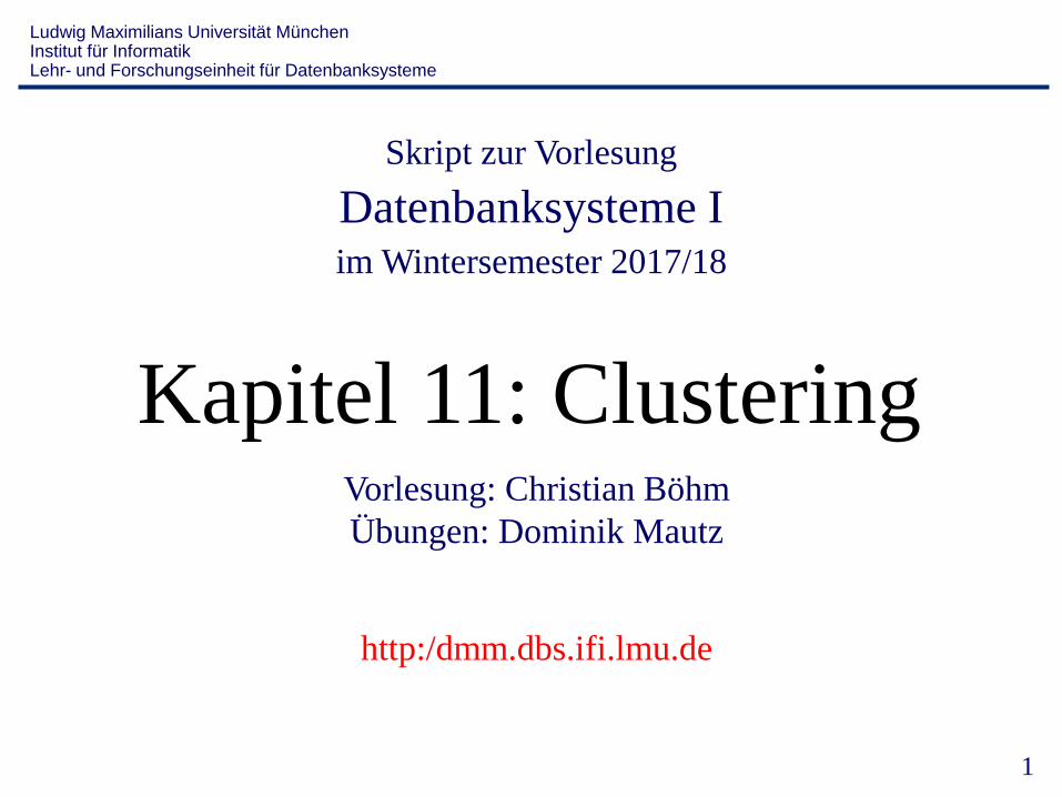
Motivation

Phone Company Astronomy

Credit Card Retail

• Big data sets are collected in databases

• Manual analysis is no more feasable

Medical Imaging

Big Data

• The buzzword “Big Data” dates back to a report by McKinsey (May 2011) (http://www.mckinsey.com/insights/business_technology/big_data_the_next_frontier_for_innovation)

• “The amount of data in our world has been exploding, and analyzing large data

sets—so-called big data—will become a key basis of competition, underpinning

new waves of productivity growth, innovation, and consumer surplus […]”

• “Data have swept into every industry and business function and are now an

important factor of production, alongside labor and capital”

– Potential Revenue in US Healthcare: > $300 Million

– Potential Revenue in public sector of EU: > €100 Million

• “There will be a shortage of talent necessary for organizations to take advantage

of big data. By 2018, the United States alone could face a shortage of 140,000 to

190,000 people with deep analytical skills as well as 1.5 million managers and

analysts with the know-how to use the analysis of big data to make effective

decisions.”

Big Data

• Data Mining is obviously an important technology to cope with Big Data

• Caution: “Big Data” does not only mean “big”

=> Three V’s (the three V’s characterizing big data)

– Volume Many objects but also huge represenations of single objects

– Velocity Data arriving in fast data streams

– Variety Not only one type of data, but different types, semi- or unstructured

4

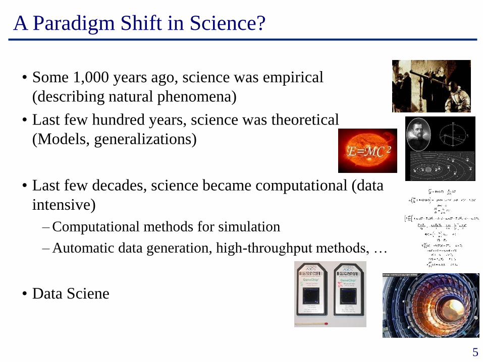
A Paradigm Shift in Science?

• Some 1,000 years ago, science was empirical

(describing natural phenomena)

• Last few hundred years, science was theoretical

(Models, generalizations)

• Last few decades, science became computational (data

intensive)

– Computational methods for simulation

– Automatic data generation, high-throughput methods, …

• Data Sciene

5

6

Definition KDD

[Fayyad, Piatetsky-Shapiro & Smyth 1996]

„Knowledge Discovery in Databases (KDD) is the nontrivial process

of identifying patterns in data which are

• valid

• novel

• potentially useful

• and ultimately understandable“

7

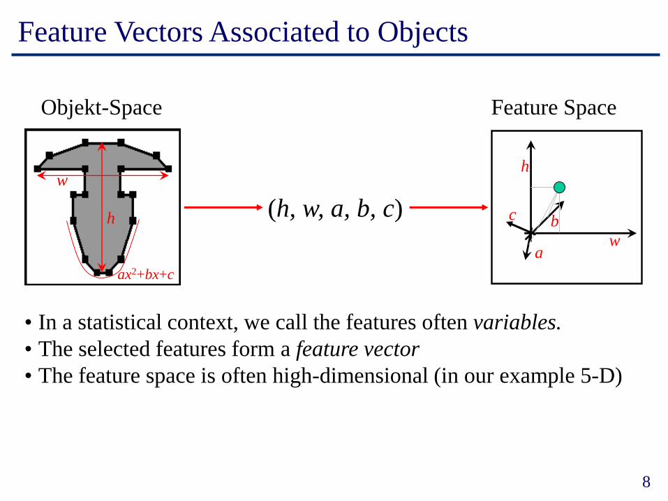
Feature Vectors Associated to Objects

• Objects of an application are often complex

• It is the task of the KDD expert to define or select suitable features

which are relevant for the distinction between various objects

Example: CAD-drawings:

Possible features:

• height h

• width w

• Curvature parameters

(a,b,c)ax2+bx+c

8

Feature Vectors Associated to Objects

(h, w, a, b, c)

ax2+bx+c

h

wh

wa

bc

Objekt-Space Feature Space

• In a statistical context, we call the features often variables.

• The selected features form a feature vector

• The feature space is often high-dimensional (in our example 5-D)

9

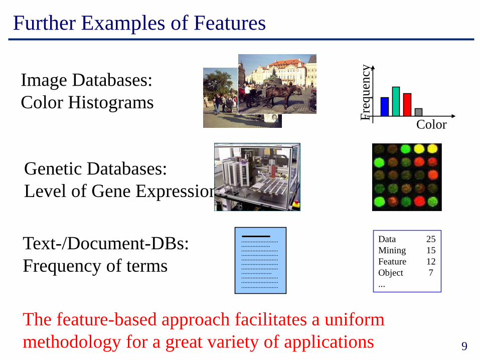
Further Examples of Features

Image Databases:

Color HistogramsColor

Fre

qu

ency

Genetic Databases:

Level of Gene Expression

Text-/Document-DBs:

Frequency of terms

The feature-based approach facilitates a uniform

methodology for a great variety of applications

Data 25

Mining 15

Feature 12

Object 7

...

10

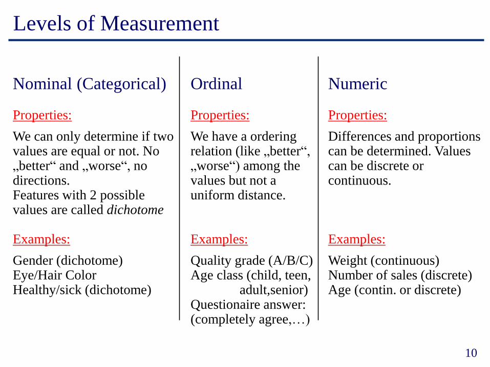
Levels of Measurement

Nominal (Categorical)

Properties:

We can only determine if twovalues are equal or not. No„better“ and „worse“, nodirections.Features with 2 possiblevalues are called dichotome

Examples:

Gender (dichotome)Eye/Hair ColorHealthy/sick (dichotome)

Ordinal

Properties:

We have a orderingrelation (like „better“, „worse“) among thevalues but not a uniform distance.

Examples:

Quality grade (A/B/C)Age class (child, teen,

adult,senior)Questionaire answer:(completely agree,…)

Numeric

Properties:

Differences and proportionscan be determined. Values can be discrete orcontinuous.

Examples:

Weight (continuous)Number of sales (discrete)Age (contin. or discrete)

11

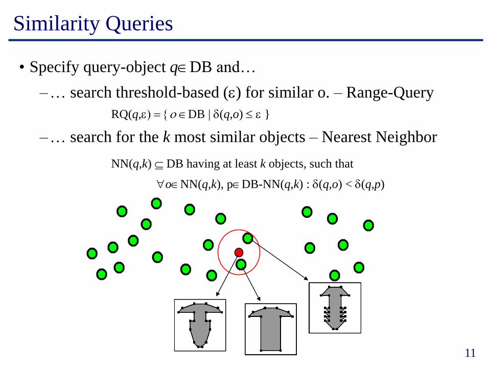
Similarity Queries

• Specify query-object qDB and…

–… search threshold-based (e) for similar o. – Range-Query

RQ(q,e) = {o DB | (q,o) e }

–… search for the k most similar objects – Nearest Neighbor

NN(q,k) DB having at least k objects, such that

oNN(q,k), pDB-NN(q,k) : (q,o) < (q,p)

12

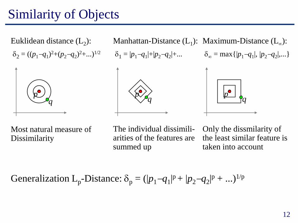
Similarity of Objects

Euklidean distance (L2):

2 = ((p1-q1)2+(p2-q2)

2+...)1/2

qp

Manhattan-Distance (L1):

1 = |p1-q1|+|p2-q2|+...

qp

Maximum-Distance (L):

= max{|p1-q1|, |p2-q2|,...}

pq

The individual dissimili-arities of the features aresummed up

Only the dissmilarity ofthe least similar feature istaken into account

Most natural measure ofDissimilarity

Generalization Lp-Distance: p = (|p1-q1|p + |p2-q2|

p + ...)1/p

13

Adaptable Similarity Measures

Weighted Euklidean distance: = (w1(p1-q1)

2 + w2(p2-q2)2+...)1/2

qp

Often the features have (heavily) varying

value ranges:

Example: Feature F1 [0.01 .. 0.05]

Feature F2 [3.1 .. 22.2]

We need a high weight for F1

(otherwise would ignore F1)

Sometimes we need a common weighting

of different features to capture

dependencies,

e.g. in color histograms to

take color similarities into account

qp

Quadratic form distance: = ((p - q) M (p - q)T )1/2

Some methods do not work with distance measures (where =0 means

equality) but with positive similarity measures (=1 means equality)

14

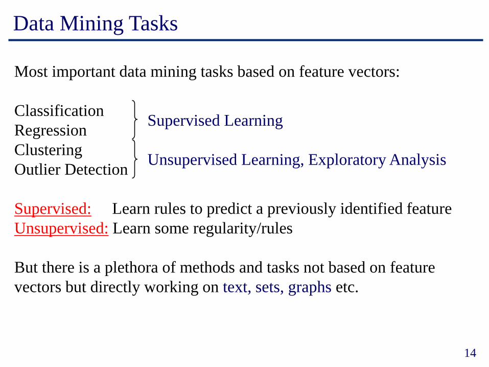
Data Mining Tasks

Most important data mining tasks based on feature vectors:

Classification

Regression

Clustering

Outlier Detection

Supervised: Learn rules to predict a previously identified feature

Unsupervised: Learn some regularity/rules

But there is a plethora of methods and tasks not based on feature

vectors but directly working on text, sets, graphs etc.

Supervised Learning

Unsupervised Learning, Exploratory Analysis

15

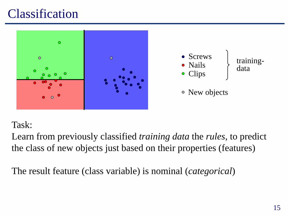
Classification

ScrewsNailsClips

Task:

Learn from previously classified training data the rules, to predict

the class of new objects just based on their properties (features)

The result feature (class variable) is nominal (categorical)

training-data

New objects

16

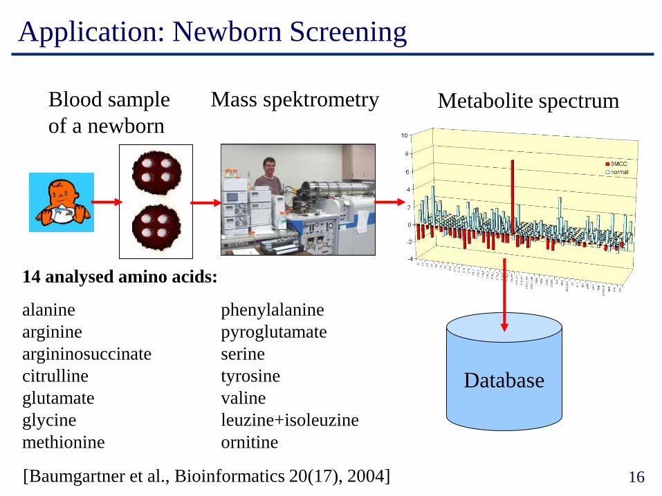
Application: Newborn Screening

Blood sample

of a newborn

Mass spektrometry Metabolite spectrum

Database

14 analysed amino acids:

alanine phenylalanine

arginine pyroglutamate

argininosuccinate serine

citrulline tyrosine

glutamate valine

glycine leuzine+isoleuzine

methionine ornitine

[Baumgartner et al., Bioinformatics 20(17), 2004]

17

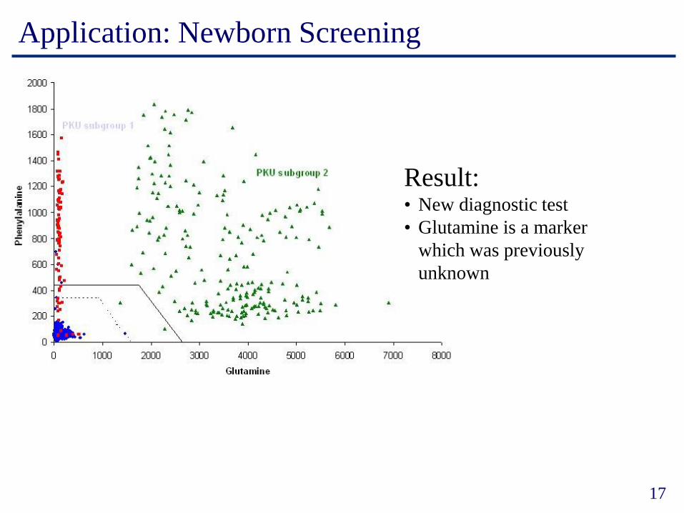
Application: Newborn Screening

Result:• New diagnostic test

• Glutamine is a marker

which was previously

unknown

18

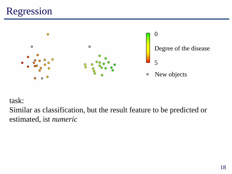
Regression

0

5

Degree of the disease

New objects

task:

Similar as classification, but the result feature to be predicted or

estimated, ist numeric

19

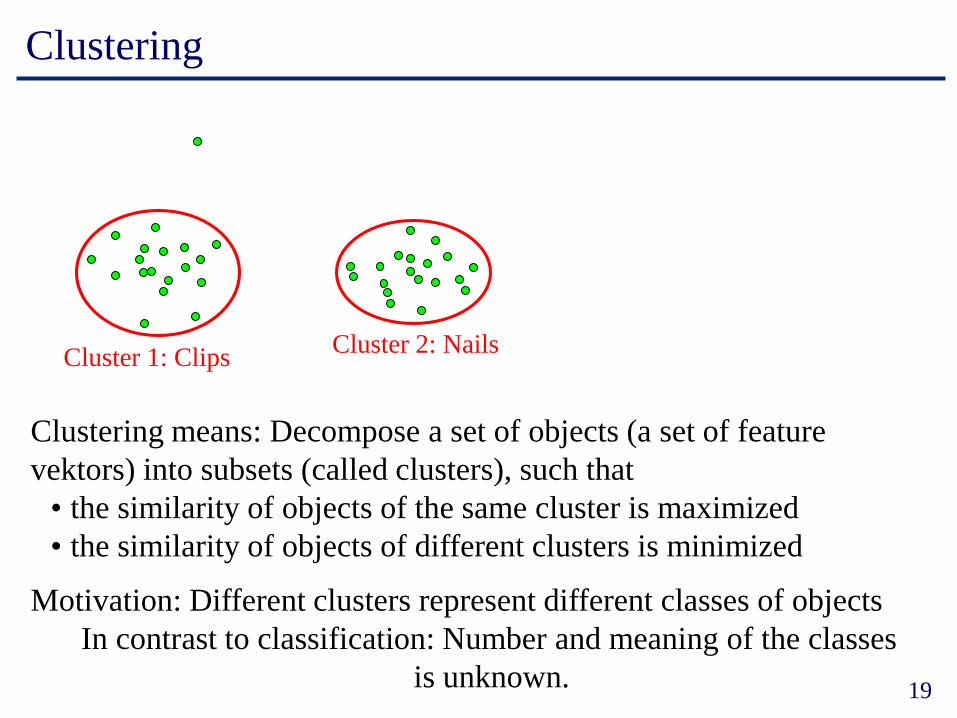
Clustering

Cluster 1: ClipsCluster 2: Nails

Clustering means: Decompose a set of objects (a set of feature

vektors) into subsets (called clusters), such that

• the similarity of objects of the same cluster is maximized

• the similarity of objects of different clusters is minimized

Motivation: Different clusters represent different classes of objects

In contrast to classification: Number and meaning of the classes

is unknown.

20

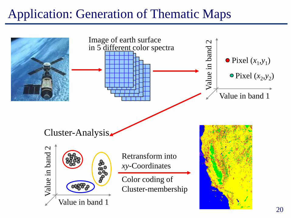
Application: Generation of Thematic Maps

Image of earth surfacein 5 different color spectra

Pixel (x1,y1)

Pixel (x2,y2)

Value in band 1

Val

ue

in b

and

2Value in band 1

Val

ue

in b

and

2

Cluster-Analysis

Retransform into

xy-Coordinates

Color coding of

Cluster-membership

21

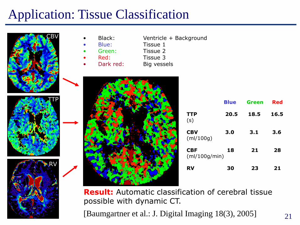
Application: Tissue Classification

RV

Result: Automatic classification of cerebral tissuepossible with dynamic CT.

• Black: Ventricle + Background• Blue: Tissue 1• Green: Tissue 2• Red: Tissue 3• Dark red: Big vessels

Blue Green Red

TTP 20.5 18.5 16.5 (s)

CBV 3.0 3.1 3.6(ml/100g)

CBF 18 21 28(ml/100g/min)

RV 30 23 21

CBV

TTP

RV

[Baumgartner et al.: J. Digital Imaging 18(3), 2005]

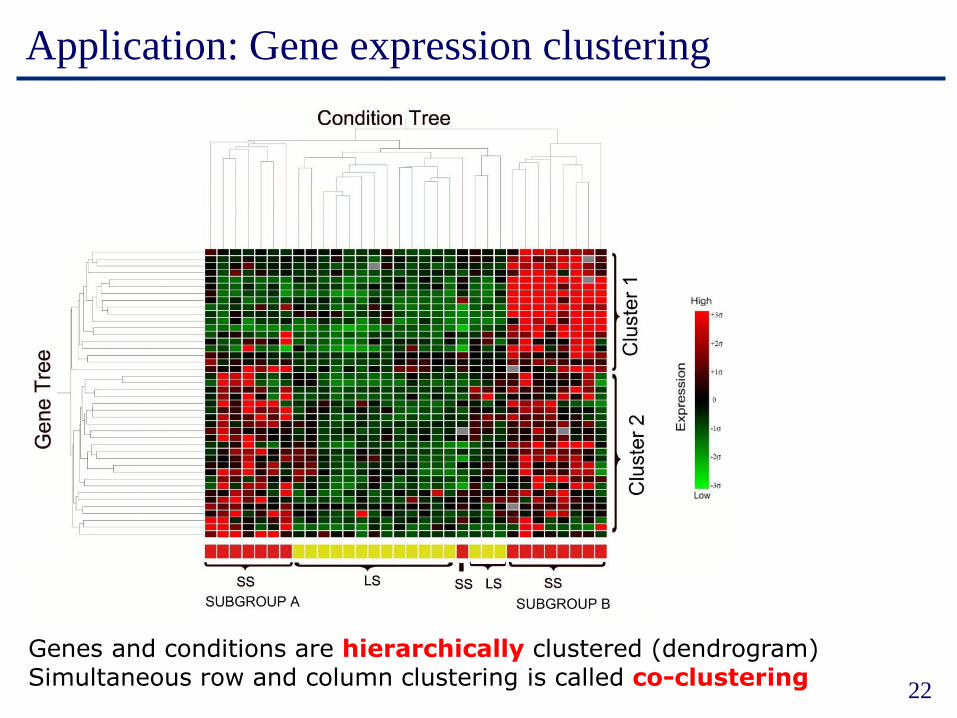
Application: Gene expression clustering

22

Genes and conditions are hierarchically clustered (dendrogram)Simultaneous row and column clustering is called co-clustering

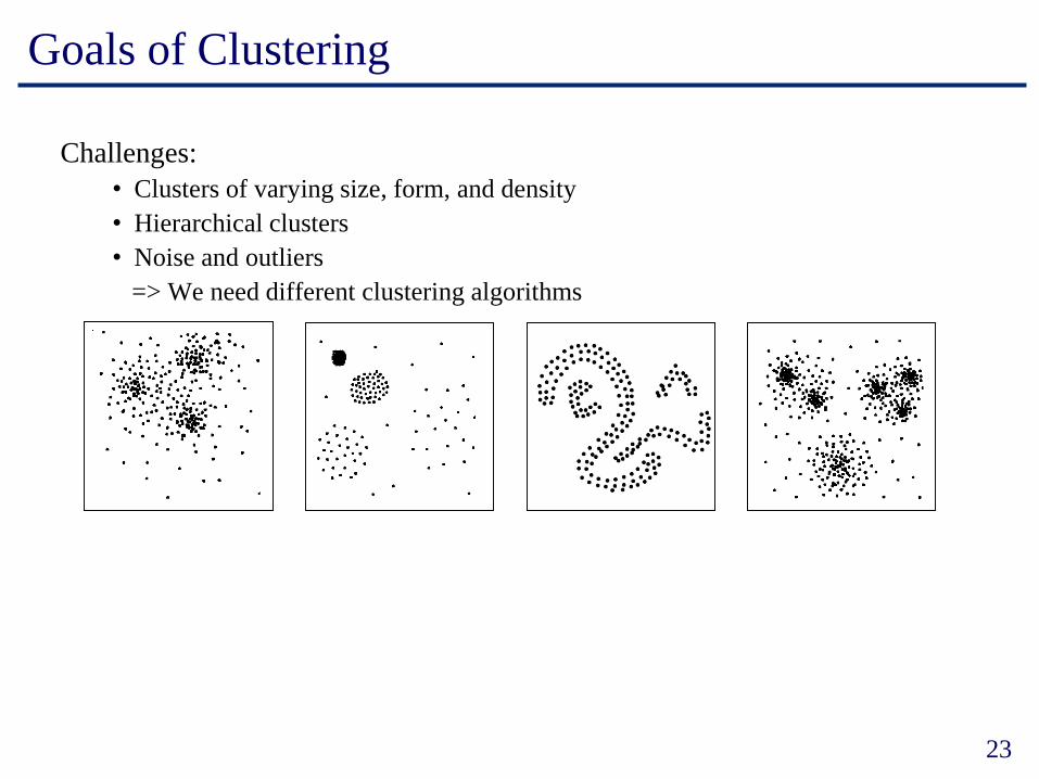
Goals of Clustering

Challenges:

• Clusters of varying size, form, and density

• Hierarchical clusters

• Noise and outliers

=> We need different clustering algorithms

23

K-Means

• Goal

– Partitioning into k clusters such that a cost function (to measure the quality) is minimized

– k is a parameter of the method (specified by user).

• Locally optimizing method

– Choose k initial cluster representatives

– Optimize these representatives iteratively

– Assign each object to its closest or most probable representative

– Repeat optimization and assignment until no more change (convergence)

• Types of cluster representants

– Center (mean, centroid) of each cluster k-means clustering

– Most central data object assinged to cluster (medoid) k-medoid clusteing

– Probability distribution of the cluster expectation maximization

[Duda, Hart: Pattern Classification and Scene Analysis, 1973]

24

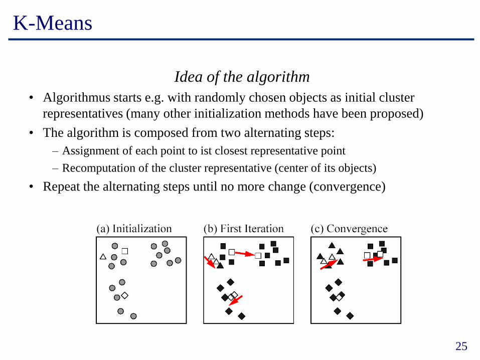
K-Means

Idea of the algorithm

• Algorithmus starts e.g. with randomly chosen objects as initial cluster

representatives (many other initialization methods have been proposed)

• The algorithm is composed from two alternating steps:

– Assignment of each point to ist closest representative point

– Recomputation of the cluster representative (center of its objects)

• Repeat the alternating steps until no more change (convergence)

25

K-Means

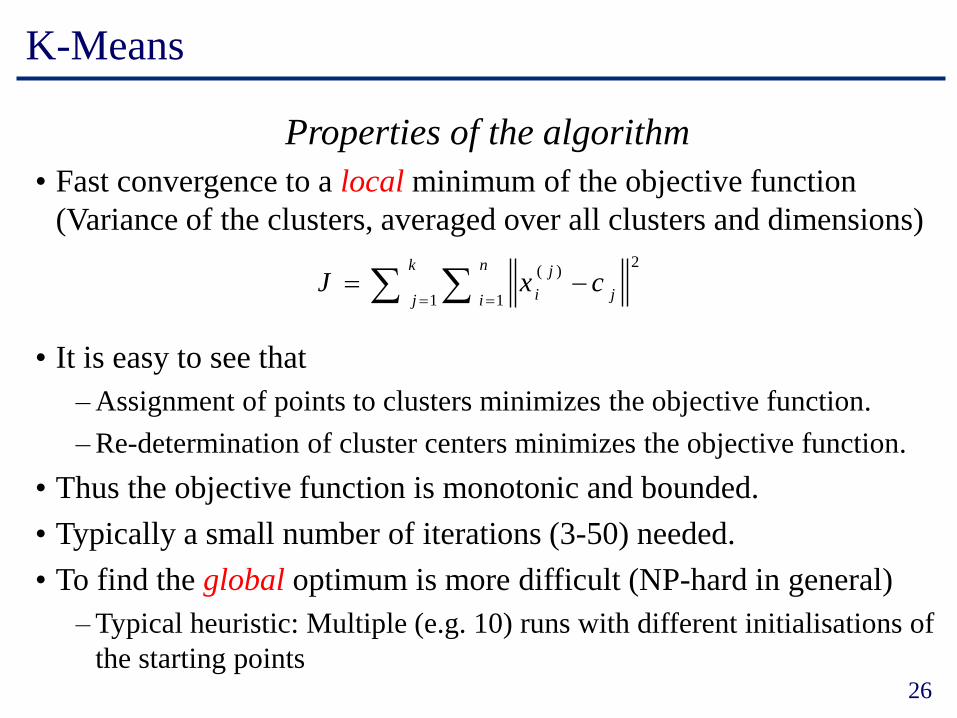
Properties of the algorithm

• Fast convergence to a local minimum of the objective function

(Variance of the clusters, averaged over all clusters and dimensions)

• It is easy to see that

– Assignment of points to clusters minimizes the objective function.

– Re-determination of cluster centers minimizes the objective function.

• Thus the objective function is monotonic and bounded.

• Typically a small number of iterations (3-50) needed.

• To find the global optimum is more difficult (NP-hard in general)

– Typical heuristic: Multiple (e.g. 10) runs with different initialisations of

the starting points26

2

1 1

)(

j

k

j

n

i

j

icxJ = =

-=

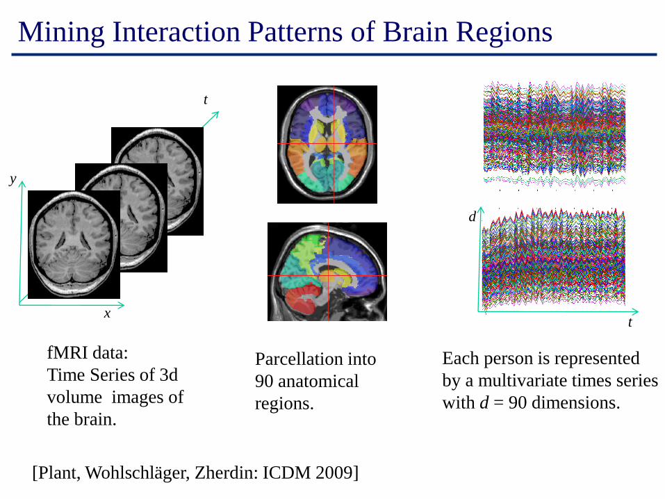
Mining Interaction Patterns of Brain Regions

Parcellation into

90 anatomical

regions.

y

fMRI data:

Time Series of 3d

volume images of

the brain.

x

t

Each person is represented

by a multivariate times series

with d = 90 dimensions.

t

d

[Plant, Wohlschläger, Zherdin: ICDM 2009]

Clustering Multivariate Time Series

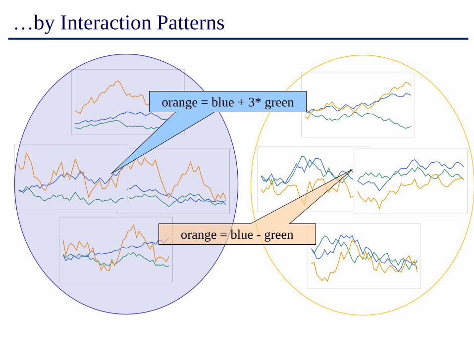
…by Interaction Patterns

orange = blue + 3* green

orange = blue - green

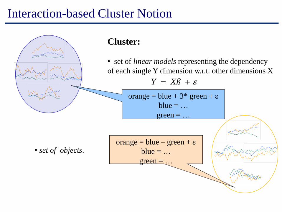
Interaction-based Cluster Notion

Cluster:

• set of linear models representing the dependency

of each single Y dimension w.r.t. other dimensions X

orange = blue + 3* green + e

blue = …

green = …

• set of objects.

e= XßY

orange = blue – green + e

blue = …

green = …

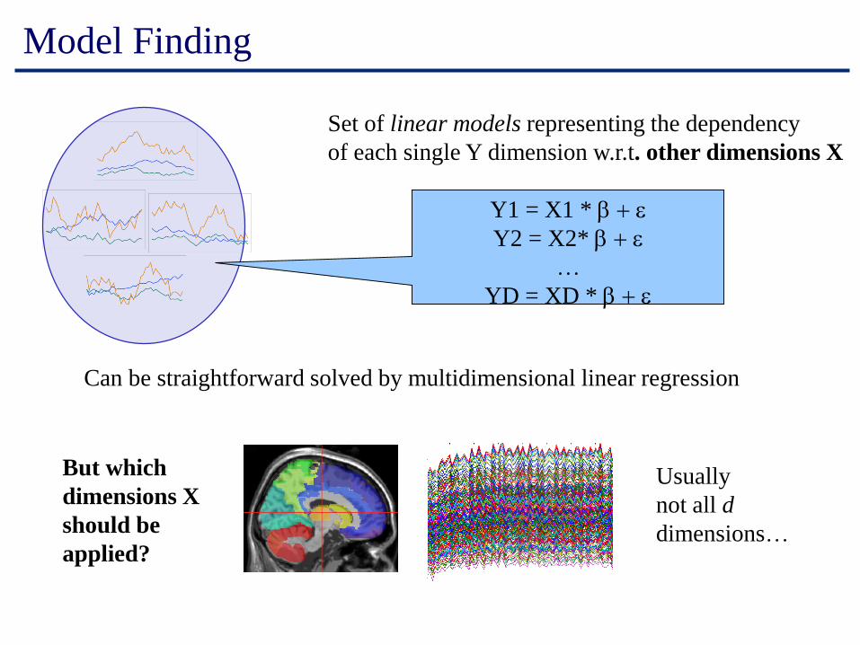
Model Finding

Set of linear models representing the dependency

of each single Y dimension w.r.t. other dimensions X

Y1 = X1 * b e

Y2 = X2* b e

…

YD = XD * b e

Can be straightforward solved by multidimensional linear regression

But which

dimensions X

should be

applied?

Usually

not all d

dimensions…

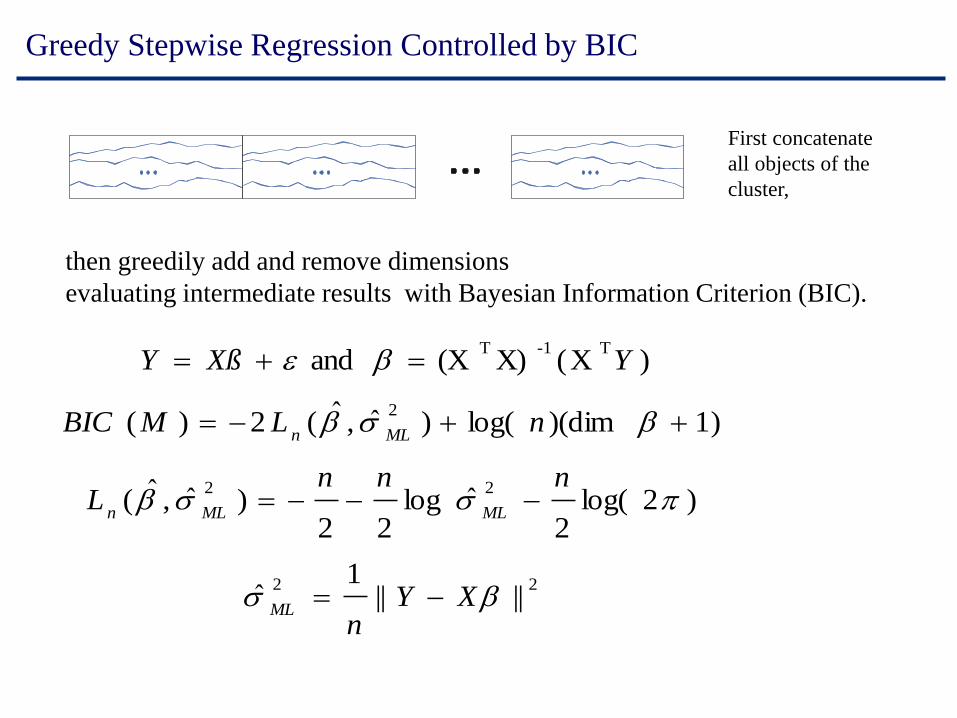
Greedy Stepwise Regression Controlled by BIC

then greedily add and remove dimensions

evaluating intermediate results with Bayesian Information Criterion (BIC).

22

22

2

T1-T

||||1

ˆ

)2log(2

ˆlog22

)ˆ,ˆ(

)1)(dimlog()ˆ,ˆ(2)(

)X(X)(X and

b

b

bb

be

XYn

nnnL

nLMBIC

YXßY

ML

MLMLn

MLn

-=

---=

-=

==

First concatenate

all objects of the

cluster,

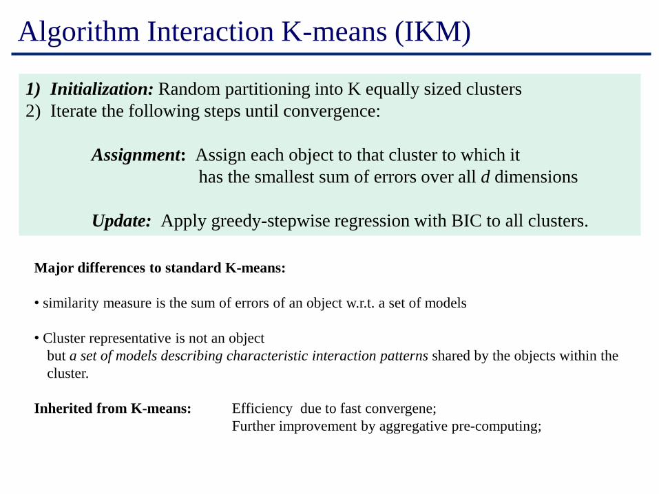
Algorithm Interaction K-means (IKM)

1) Initialization: Random partitioning into K equally sized clusters

2) Iterate the following steps until convergence:

Assignment: Assign each object to that cluster to which it

has the smallest sum of errors over all d dimensions

Update: Apply greedy-stepwise regression with BIC to all clusters.

Major differences to standard K-means:

• similarity measure is the sum of errors of an object w.r.t. a set of models

• Cluster representative is not an object

but a set of models describing characteristic interaction patterns shared by the objects within the

cluster.

Inherited from K-means: Efficiency due to fast convergene;

Further improvement by aggregative pre-computing;

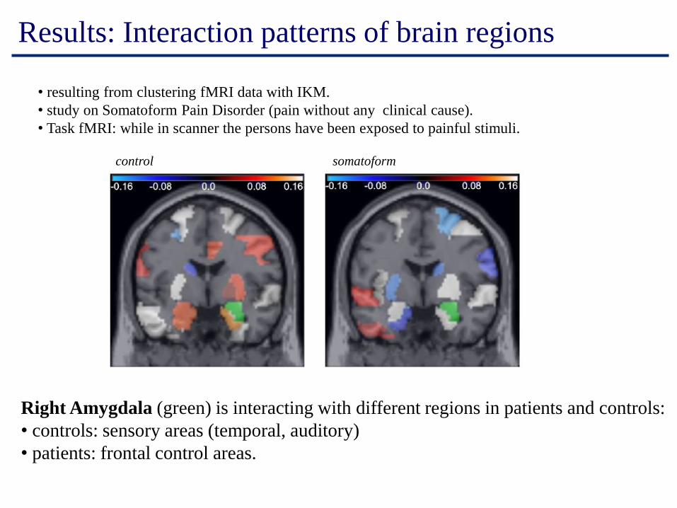
Results: Interaction patterns of brain regions

control somatoform

• resulting from clustering fMRI data with IKM.

• study on Somatoform Pain Disorder (pain without any clinical cause).

• Task fMRI: while in scanner the persons have been exposed to painful stimuli.

Right Amygdala (green) is interacting with different regions in patients and controls:

• controls: sensory areas (temporal, auditory)

• patients: frontal control areas.

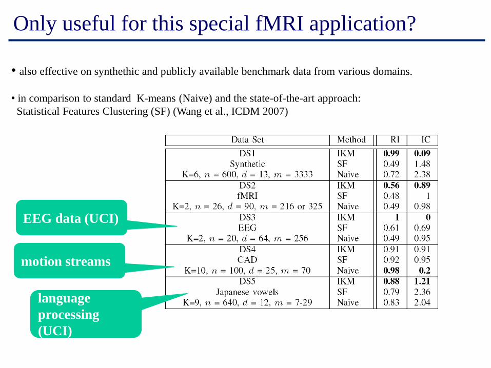
Only useful for this special fMRI application?

• also effective on synthethic and publicly available benchmark data from various domains.

• in comparison to standard K-means (Naive) and the state-of-the-art approach:

Statistical Features Clustering (SF) (Wang et al., ICDM 2007)

EEG data (UCI)

motion streams

language

processing

(UCI)

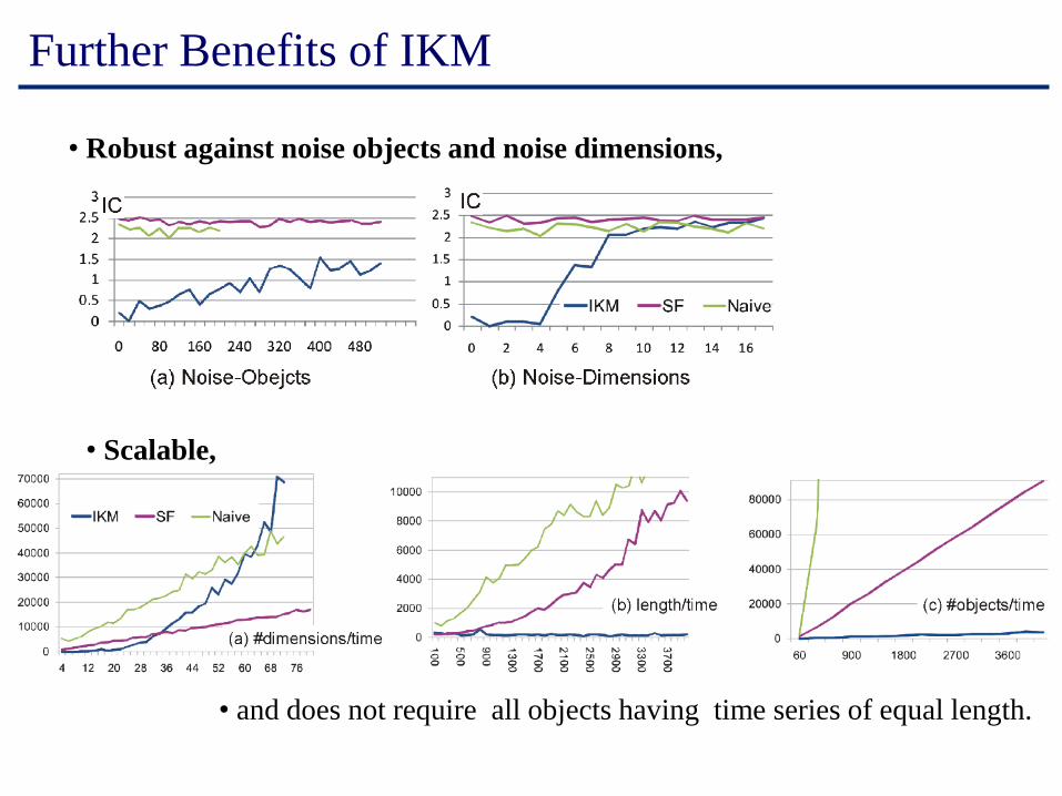
Further Benefits of IKM

• Robust against noise objects and noise dimensions,

• Scalable,

• and does not require all objects having time series of equal length.

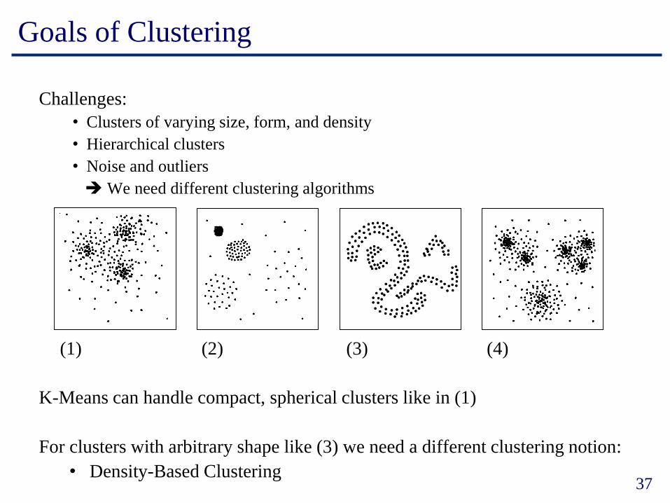
Goals of Clustering

Challenges:

• Clusters of varying size, form, and density

• Hierarchical clusters

• Noise and outliers

We need different clustering algorithms

37

K-Means can handle compact, spherical clusters like in (1)

For clusters with arbitrary shape like (3) we need a different clustering notion:

• Density-Based Clustering

(1) (2) (3) (4)

O

Q

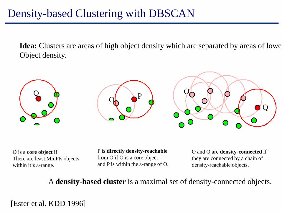
Density-based Clustering with DBSCAN

Idea: Clusters are areas of high object density which are separated by areas of lower

Object density.

O is a core object if

There are least MinPts objects

within it‘s e-range.

OO

P

P is directly density-reachable

from O if O is a core object

and P is within the e-range of O.

O and Q are density-connected if

they are connected by a chain of

density-reachable objects.

A density-based cluster is a maximal set of density-connected objects.

[Ester et al. KDD 1996]

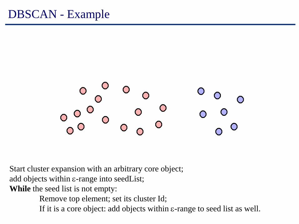
DBSCAN - Example

Start cluster expansion with an arbitrary core object;

add objects within e-range into seedList;

While the seed list is not empty:

Remove top element; set its cluster Id;

If it is a core object: add objects within e-range to seed list as well.

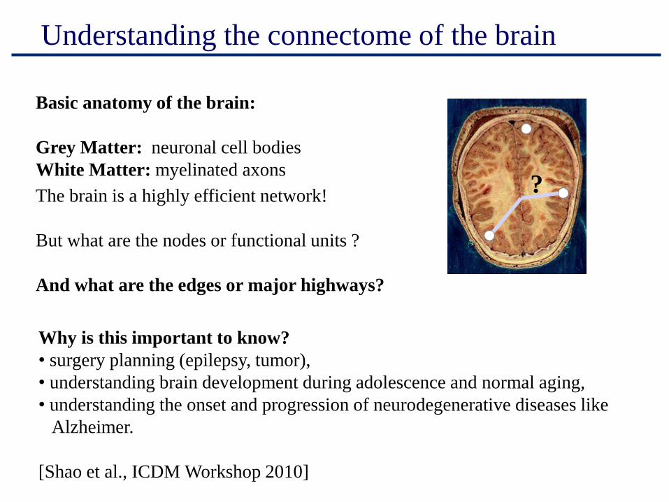
Understanding the connectome of the brain

Basic anatomy of the brain:

Grey Matter: neuronal cell bodies

White Matter: myelinated axons

The brain is a highly efficient network!

But what are the nodes or functional units ?

And what are the edges or major highways?

?

Why is this important to know?

• surgery planning (epilepsy, tumor),

• understanding brain development during adolescence and normal aging,

• understanding the onset and progression of neurodegenerative diseases like

Alzheimer.

[Shao et al., ICDM Workshop 2010]

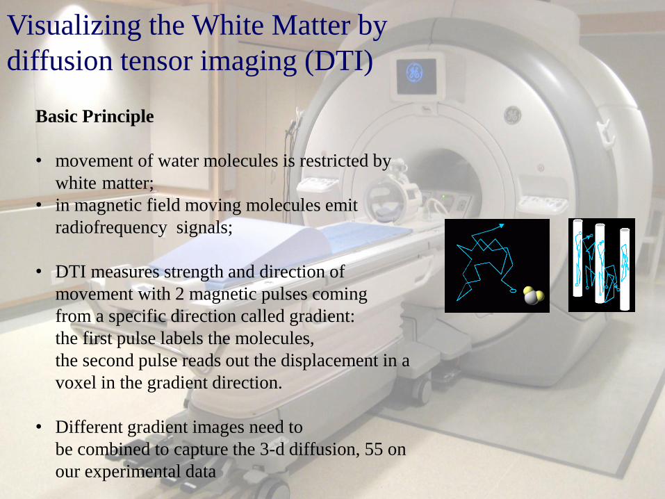
Visualizing the White Matter by

diffusion tensor imaging (DTI)

Basic Principle

• movement of water molecules is restricted by

white matter;

• in magnetic field moving molecules emit

radiofrequency signals;

• DTI measures strength and direction of

movement with 2 magnetic pulses coming

from a specific direction called gradient:

the first pulse labels the molecules,

the second pulse reads out the displacement in a

voxel in the gradient direction.

• Different gradient images need to

be combined to capture the 3-d diffusion, 55 on

our experimental data

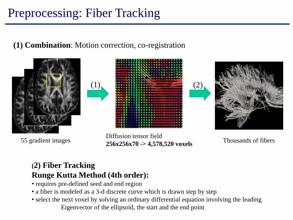
(1) Combination: Motion correction, co-registration

(2) Fiber Tracking

Runge Kutta Method (4th order):• requires pre-defined seed and end region

• a fiber is modeled as a 3-d discrete curve which is drawn step by step

• select the next voxel by solving an ordinary differential equation involving the leading

Eigenvector of the ellipsoid, the start and the end point

(1)

55 gradient imagesDiffusion tensor field

256x256x70 -> 4,578,520 voxels

(2)

Thousands of fibers

Preprocessing: Fiber Tracking

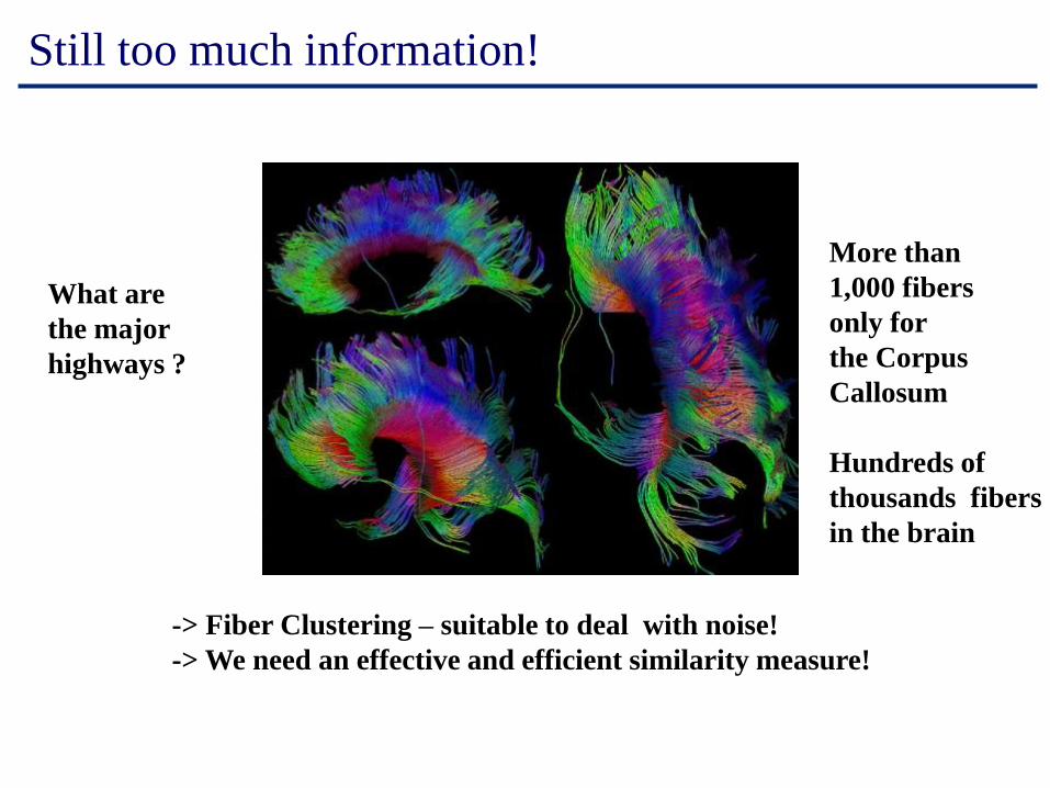
Still too much information!

What are

the major

highways ?

More than

1,000 fibers

only for

the Corpus

Callosum

Hundreds of

thousands fibers

in the brain

-> Fiber Clustering – suitable to deal with noise!

-> We need an effective and efficient similarity measure!

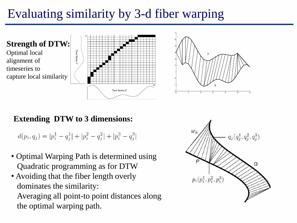
Evaluating similarity by 3-d fiber warping

Strength of DTW:Optimal local

alignment of

timeseries to

capture local similarity

Extending DTW to 3 dimensions:

• Optimal Warping Path is determined using

Quadratic programming as for DTW

•Avoiding that the fiber length overly

dominates the similarity:

Averaging all point-to point distances along

the optimal warping path.

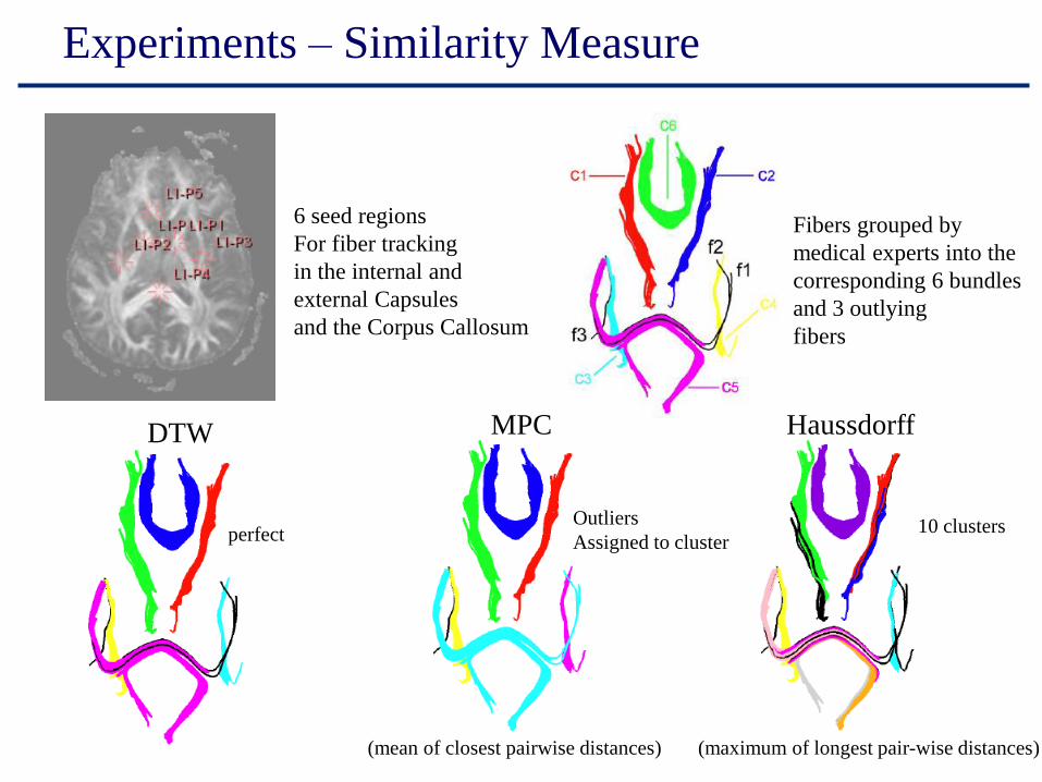
Experiments – Similarity Measure

6 seed regions

For fiber tracking

in the internal and

external Capsules

and the Corpus Callosum

Fibers grouped by

medical experts into the

corresponding 6 bundles

and 3 outlying

fibers

DTW MPC Haussdorff

Outliers

Assigned to cluster10 clustersperfect

(mean of closest pairwise distances) (maximum of longest pair-wise distances)

Effective detection of clusters of different size and

separation of noise DBSCAN is good!

Data Set 2: 973 fibers

Results

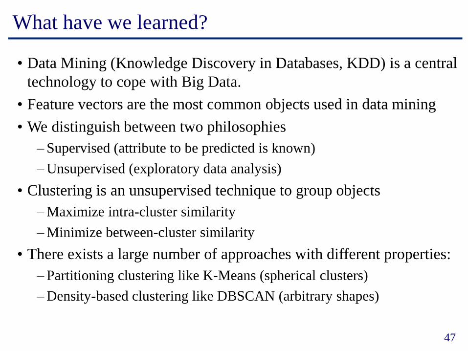
What have we learned?

• Data Mining (Knowledge Discovery in Databases, KDD) is a central

technology to cope with Big Data.

• Feature vectors are the most common objects used in data mining

• We distinguish between two philosophies

– Supervised (attribute to be predicted is known)

– Unsupervised (exploratory data analysis)

• Clustering is an unsupervised technique to group objects

– Maximize intra-cluster similarity

– Minimize between-cluster similarity

• There exists a large number of approaches with different properties:

– Partitioning clustering like K-Means (spherical clusters)

– Density-based clustering like DBSCAN (arbitrary shapes)

47