Embed Size (px)
Citation preview

PhD Thesis:Passive Fluid Management in
Micro Direct Methanol Fuel Cells
Christian Litterst
18. Mai 2009
Dissertation zur Erlangung des Doktorgradesder Technischen Fakultat der Albert-Ludwigs Universitat
Freiburg im Breisgau.


DekanProf. Dr. Hans Zappe (Freiburg)
ReferentenProf. Dr. Roland Zengerle (Freiburg)Prof. Dr. Holger Reinecke (Freiburg)
Tag der Prufung13. Januar 2010
Institut fur Mikrosystemtechnik (IMTEK)Lehrstuhl fur AnwendungsentwicklungTechnische FakultatAlbert-Ludwigs-Universitat Freiburg
I

Summary
This thesis describes the development of a passive micro direct methanolfuel cell (µDMFC) with stable runtime over 15 hours. The passive µDMFCis a combination of a state-of-the-art passive cathode design with a newlydeveloped passive anode fuel supply method. This method is based on aliquid flow rate generated by passive gas bubble removal. Starting froma theoretical evaluation of active and passive anode methanol supply andgas bubble removal methods, four different flow field channel designs aredeveloped and studied using analytical, numerical and experimental methods.Based on the presented results, a new fuel cell system design is proposedthat allows long term passive operation while providing small overall systemdimensions.
A unit single cell is identified as best architecture for the studies in thiswork. A theoretical evaluation of fuel supply and waste removal concepts ofthe anode side is presented in Chapter 2. Based on the presented concepts,four different flow field channel designs are manufactured: one reference (typeR) with rectangular channel layout and three designs (types A, B and C )with different tapered profiles. Tapered channel designs are chosen sinceelongated gas bubbles start to move towards the wider part of a taperedchannel. This movement is a consequence of different capillary pressures atthe distant ends of a gas bubble and allows to passively remove the gas bubblefrom the anode. Channel type A is tapered along its length axis; type B isT-shaped and tapered along its axis and symmetric at its cross-section andtype C is a planar channel geometry tapered along its cross-section.
A reference fuel cell design with continuous active fuel supply and waste re-moval was used as reference for all experiments. Its mean power density wasmeasured and yields Pref,lrr = 1.5mWcm−2. The step to a newly proposeddiscontinuous pump operation with regular intervals of 0.5min active pump-ing and 9.5min passive fuel cell operation over a period of 15 intervals yields
III

Summary
a significant mean performance improvement for all three channel types by1.7–2.9× against the reference cell. This new approach can be implementedinto persisting active fuel cell systems to improve their performance. Thepassive pumping by capillary forces is verified by studying single flow fieldchannels in simulation and experiments. This is done by artificial bubblecreation and comparing the results with the theoretical minimum requiredpump efficiency of ηpump = φMeOH ,sol
φCO2= 1%. Flow rate measurements in pas-
sive µDMFC operation proof that passive removal of CO2 gas bubbles andpumping of methanol can be achieved. In the experiments all three chan-nel types show pumping efficiencies of ηpump,R = 16%, ηpump,A = 13% andηpump,B = 5% which are significantly above the minimum required efficiency.
Since in the experiments with passive fuel cell operation all provided methanolis utilized, the fuel cells energy efficiency as ratio of the gathered electrical en-ergy and the provided chemical energy can be determined. In the experimentswith 2.0mL, 3.1mL and 9.1mL reservoir filling volume energy efficiencies of6–13% are achieved with increased mean power densities of 1.2–2× againstthe reference. Furthermore, a linear correlation between the runtime of thefuel cell and the provided amount of fuel is demonstrated. This correlationindicates that the fuel amount is the limiting factor of the runtime and vali-dates that the bubble induced fuel recirculation is a long term stable processwhich results in a runtime of more than 15 hours for 9.1mL of 4M methanolsolution. A further increase of the system energy density can be achievedby re-dosing pure methanol at intervals into a small reservoir. The meanpower densities measured with this approach exceed the reference value by1.5–1.9×.
IV

Zusammenfassung
Diese Arbeit beschreibt die Entwicklung einer passiven Mikro-Direktmetha-nolbrennstoffzelle (µDMFC) mit einer kontinuierlichen, stabilen Laufzeit uber15 Stunden. Der Aufbau der passiven µDMFC besteht aus der Kombinationeines passiven Anodenaufbaus nach dem Stand der Technik und einer neuar-tigen anodenseitigen Brennstoffversorgung. Mit Hilfe einer durch die passiveEntfernung von Gasblasen erzeugten Flussrate wird der Brennstoffzelle fri-sches Methanol zugefuhrt. Ausgehend von einer theoretischen Betrachtungverschiedener Methoden zur Brennstoffversorgung und Entfernung der Gas-blasen werden vier verschiedene Kanalformen fur das anodenseitige Flowfieldentwickelt und analytisch, numerisch und experimentell untersucht. Auf-bauend auf die erzielten Erkenntnisse wird ein neues Design eines µDMFC-Systems vorgeschlagen, das einen stabilen Betrieb uber einen langen Zeitraumerlaubt und gleichzeitig die benotigte Systembaugroße reduziert.
Fur den Systemaufbau wird in dieser Arbeit eine einzelne Brennstoffzelle(Unit Singel Cell) gewahlt. Verschiedene Konzepte zu ihrer Brennstoffversor-gung und zum Entfernen der Gasblasen werden dazu in Kapitel 2 theoretischbetrachtet. Aus dieser Untersuchung hervorgehend werden vier verschiedeneKanalformen entwickelt und hergestellt: ein Referenzkanal (Typ R) mit recht-eckigem Querschnitt und drei weitere Kanale (Typ A, B und C ) mit unter-schiedlichen Keilformen entlang ihrer Langsachse. Der keilformige Kanalauf-bau fuhrt bei ausgedehnten Gasblasen zu einer Bewegung in Richtung desgroßeren Kanalquerschnitts. Die Bewegung resultiert aus den unterschied-lichen Kapillardrucken an den Enden der Gasblase und diese konnen somitpassiv von der Anode entfernt werden. Die Kanalformen unterscheiden sichfolgendermaßen: Bei Typ A nimmt die Hohe des rechteckigen Querschnittsuber die Kanallange zu. Typ B hat ein T-formigen Querschnitt dessen Sei-tenarme ein keilformiges Profil aufweisen. Die Hohe nimmt ebenfalls mit derKanallange zu. Typ C ist ein flacher Kanal, dessen Breite uber die Langezunimmt.
V

Zusammenfassung
Ein Systemaufbau mit kontinuierlich gepumpter Brennstoffzufuhr und Ent-fernung der Gasblasen dient als Referenz fur alle weiteren Versuche. Die mitt-lere Leistungsdichte dieses Referenzaufbaus betragt Pref,lrr = 1.5mWcm−2.Mit dem neu vorgeschlagenen Betriebsmodus des diskontinuierlichen Pum-pens mit regelmaßigen 0.5 minutigen Pumpintervallen und 9.5 minutigempassiven Betrieb der µDMFC uber einen Zeitraum von 15 Intervallen wirdeine deutliche Verbesserung der mittleren Leistungsdichte um das 1.7–2.9-fache im Vergleich zum Referenzwert erzielt. Dieser neue Betriebsmoduskann auch in existierenden System eingesetzt werden um deren Effizienz zuverbessern. Das passive Pumpen mit Hilfe der Kapillarkrafte wird zunachstmit Simulationen und Experimenten an einem einzelnen Kanal des Flow-fields nachgewiesen. In diesen Experimenten werden die Gasblasen in denKanal injiziert und die resultierende Flussrate mit dem minimal benotig-ten Pumpwirkungsgrad ηpump = φMeOH,sol
φCO2= 1% verglichen. Messungen der
Flussrate wahrend des passiven Brennstoffzellenbetriebs zeigen, dass die pas-sive Entfernung der CO2 Gasblasen und das gleichzeitige Pumpen der Me-thanollosung auch im realen Brennstoffzellensystem funktioniert. Der Pump-wirkungsgrad ist fur alle drei Kanaltypen mit ηpump,R = 16%, ηpump,A = 13%und ηpump,B = 5% deutlich uber dem minimal benotigten Pumpwirkungsgradvon 1%.
Fur den passiven Systemaufbau kann der Wirkungsgrad der Brennstoffzelleals Verhaltnis der generierten elektrischen Energy und der zur Verfugung ge-stellten chemischen Energie bestimmt werden, da theoretisch das kompletteVolumen an Methanol in elektrische Energie umgesetzt werden kann. Inden Experimenten mit 2.0ml, 3.1ml and 9.1ml Methanollosung werden Wir-kungsgrade im Bereich von 6–13% erreicht. Dabei ubersteigen die mittlerenLeistungsdichten den Referenzwert um das 1.2–2-fache. Zudem besteht einlinearer Zusammenhang zwischen der Laufzeit der DMFC und der Mengean Methanollosung. Dieser Zusammenhang zeigt, dass die Menge an Metha-nollosung die Laufzeit der Zelle limitiert und das passive Pumpen mit Hilfeder Gasblasen ein uber lange Zeit stabiler Prozess ist. Mit 9.1ml einer 4molaren Methanollosung werden stabile Laufzeiten uber 15 Stunden erreicht.Eine Steigerung der Energiedichte des Systems kann durch intervallweisesnachdosieren von Methanol in ein kleines Reservoir mit Methanollosung er-zielt werden. Experimente, die dieses Vorgehen nutzen fuhren zu mittlerenLeistungsdichten die den Referenzwert um 1.5–1.9× ubersteigen.
VI
Patents and publications
Parts of this work have been published in patents, journals and conferencesor are related to it. These publications are indicated by a leading *-symbol.
Patents
[I] *S. Eccarius, C. Litterst, and P. Koltay. (EN) Method for operat-ing a direct oxidation fuel cell and corresponding arrangement; (DE)Verfahren zum Betreiben einer Direktoxidationsbrennstoffzelle und ent-sprechende Anordnung. Nov 2007. Pub. No.: WO/2007/060020; In-ternational Application No.: PCT/EP2006/011421.
[II] *S. Eccarius, C. Litterst, and P. Koltay. Direct-oxidation fuel cellwith passive fuel supply and method for its operation; (DE) Direktoxi-dationsbrennstoffzelle mit passiver Brennstoffzufuhrung und Verfahrenzu deren Betreiben. Jan 2007. Pub. No.: WO/2007/085402; Interna-tional Application No.: PCT/EP2007/000518.
[III] *P. Koltay, C. Litterst, and S. Eccarius. Device comprising a channelcarrying a medium and method for removing inclusions; (DE) Vor-richtung mit einem ein Medium fuhrenden Kanal und Verfahren zurEntfernung von Einschlussen. Jan 2006. Pub. No.: WO/2006/082087;International Application No.: PCT/EP2006/000990.
Journal publications
[IV] *N. Paust, C. Litterst, T. Metz, M. Eck, C. Ziegler, R. Zengerle,and P. Koltay. Capillary-driven pumping for passive degassing and fuelsupply in direct methanol fuel cells. Microfluidics and Nanofluidics,2009. DOI 10.1007/s10404-009-0414-9.
VII

Patents and publications
[V] *C. Litterst, T. Metz, R. Zengerle, and P. Koltay. Static and dynamicbehaviour of gas bubbles in T-shaped non-clogging micro-channels. Mi-crofluidics and Nanofluidics, 5(6)775–784, 2008. DOI 10.1007/s10404-008-0279-3.
[VI] *T. Glatzel, C. Cupelli, T. Lindemann, C. Litterst, Ch. Moosmann,R. Niekrawietz, W. Streule, R. Zengerle, and P. Koltay. Computationalfluid dynamics (CFD) software tools for microfluidic applications - Acase study. Computers & Fluids, 37(3):218-235, 2008.
[VII] *C. Litterst, S. Eccarius, C. Hebling, R. Zengerle, and P. Koltay. In-creasing µDMFC efficiency by passive CO2 bubble removal and discon-tinuous operation. Journal of Micromechanics and Microengineering,16(9):S248-S253, 2006.
Conference publications
[VIII] *N. Paust, C. Litterst, T. Metz, R. Zengerle, and P. Koltay. Fullypassive degassing and fuel supply in direct methanol fuel cells. In Pro-ceedings of the 21st IEEE International Conference on Micro ElectroMechanical Systems, MEMS, pages 34-37. 2008.
[IX] *N. Paust, C. Litterst, T. Metz, M. Eck, R. Zengerle, and P. Koltay.Capillary driven fuel supply in direct methanol fuel cells with doubletapered T-shaped channel flow fields. In Proceedings of PowerMEMS2007, pages 185-188. 2007.
[X] *N. Paust, C. Litterst, T. Metz, R. Zengerle, and P. Koltay. Gas-blasengetriebene Pumpe fur Mikroreaktoren. In VDI-VDE-IT, edi-tor, Proceedings of Mikrosystemtechnik-Kongress, pages 481-484. VDEVerlag, Oct 2007.
[XI] *C. Litterst, S. Eccarius, C. Hebling, R. Zengerle, and P. Koltay.Novel Structure for Passive CO2 Degassing in µDMFC. In Proceedingsof IEEE MEMS 2006, pages 102–105. Istanbul, Turkey, 2006.
VIII

[XII] *C. Litterst, S. Eccarius, C. Hebling, R. Zengerle, and P. Koltay.Novel Structure for Passive CO2 Degassing in µDMFC. In Proceedingsof PowerMEMS 2005, pages 194–197. Tokyo, 2005.
[XIII] *S. Eccarius, C. Litterst, A. Wolff, M. Tranitz, P. Koltay, and C.Agert. Systemaspekte in planaren Mikrobrennstoffzellensystemen. InProceedings of Mikrosystemtechnik-Kongress 2005, pages 713–716.Freiburg, 2005.
[XIV] C. Litterst, W. Streule, P. Koltay, and R. Zengerle. Simulation Toolkitfor Micro-Fluidic Pumps using Lumped Models. In Technical Proceed-ings of the 2005 Nanotechnology Conference and Trade Show, pages736–739. Anaheim, 2005.
[XV] *C. Litterst, J. Kohnle, H. Ernst, S. Messner, H. Sandmaier, R.Zengerle, and P. Koltay. Improved gas bubble mobility in CHIC-typeflow channels. In Hubert Borgmann, editor, ACTUATOR, pages 541–544. 2004.
[XVI] P. Koltay, S. Taoufik, C. Litterst, J. Hansen-Schmidt, and R. Zengerle.Simulation of micro dispensing devices. In Proceedings of 20th CAD-FEM Users’ Meeting, International Congress on FEM-Technology.Friedrichshafen, 2002.
[XVII] P. Koltay, C. Moosmann, C. Litterst, W. Streule, B. Birkenmaier,and R. Zengerle. Modelling free jet ejection on a system level - anapproach for microfluidics. In Proceedings of Fifth International Con-ference on Modeling and Simulation of Microsystems (MSM), pages170–173. April 22–25, San Juan, Puerto Rico, USA, 2002.
[XVIII] P. Koltay, C. Moosmann, C. Litterst, W. Streule, and R. Zengerle.Simulation of a micro dispenser using lumped models. In Proceed-ings of Fifth International Conference on Modeling and Simulation ofMicrosystems (MSM), pages 112–115. April 22–25, San Juan, PuertoRico, USA, 2002.
IX

Contents
Summary III
Zusammenfassung V
Patents and publications VII
1 Introduction 11.1 Working principle of Direct Methanol Fuel Cells . . . . . . . 31.2 State-of-the-art in µDMFC development . . . . . . . . . . . . 91.3 Aim and structure of the thesis . . . . . . . . . . . . . . . . . 17
2 Concepts for passive fluid management 212.1 Active versus passive fuel cell systems . . . . . . . . . . . . . 222.2 Flow field design for passive systems . . . . . . . . . . . . . . 252.3 Concepts for gas bubble removal based on capillary forces . . 262.4 Diffusion driven concepts for fuel supply . . . . . . . . . . . . 32
3 Experimental setup and reference fuel cell 373.1 Fuel cell manufacturing and assembly . . . . . . . . . . . . . 373.2 Assembly for bubble induced pumping studies . . . . . . . . . 443.3 Experimental setup . . . . . . . . . . . . . . . . . . . . . . . . 443.4 Experimental results with active pumping . . . . . . . . . . . 49
4 Passive pumping in simulation and experiment 634.1 CFD-modeling . . . . . . . . . . . . . . . . . . . . . . . . . . 634.2 Required methanol flow for continuous passive fuel cell operation 694.3 Flow rate studies in simulations . . . . . . . . . . . . . . . . . 714.4 Flow rate studies in experiments . . . . . . . . . . . . . . . . 774.5 Bubble induced methanol supply of µDMFC . . . . . . . . . . 83
XI

Contents
5 Passive fuel cell designs driven by capillary forces 915.1 Passive flow field design / Experimental setup . . . . . . . . . 915.2 Experiments with capillary fuel supply . . . . . . . . . . . . . 94
6 Summary and outlook 1096.1 Design guidelines . . . . . . . . . . . . . . . . . . . . . . . . . 112
Bibliography 113
A Glossary 125
B Design parameters and dimensions 129
C Picture sequences 133
Acknowledgements 139
XII

1 Introduction
This first chapter of the thesis comprises an introduction to the direct meth-anol fuel cell (DMFC), the class of energy source it belongs to, the recentdevelopments and market analysis in this field especially focussed on theuse as energy source for portable applications. Furthermore the chemicalreactions in a DMFC and typical system architectures are discussed. Thisknowledge is used as basis for the development of a passive micro directmethanol fuel cell (µDMFC) system outlined at the end of this chapter anddiscussed in detail in the following chapters.
The µDMFC as alternative energy source to batteries for portableapplications
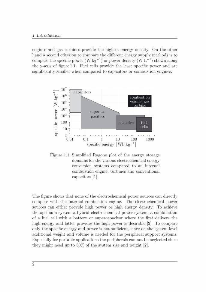
Throughout the recent years there have been a lot of new products in the fieldof portable consumer electronics like mobile phones, MP3-players and GPS-receivers, among others. All these devices have to be supplied with electricalenergy which is commonly done via Lithium-Ion batteries. These batter-ies belong to the family of power sources that are based on electrochemicalreactions. The same family includes electrochemical capacitors, like superca-pacitors. Besides this classical kind of energy supply there are attempts todevelop alternative energy sources. One of the most promising types of al-ternative energy source for portable electronics is the fuel cell, especially thedirect methanol fuel cell [1, 2]. Whereas batteries are well established in themarkets and cover a very wide range of products, fuel cells for portable elec-tronics are basically still in the development stage and so far few applicationshave been found where they can compete with or even replace batteries. Oncein mass production, it is expected that the costs for fuel cells will be in thesame order as batteries but with a higher specific energy density. As shown infigure 1.1, which is known as Ragone plot, fuel cells, conventional combustion
1
1 Introduction
engines and gas turbines provide the highest energy density. On the otherhand a second criterion to compare the different energy supply methods is tocompare the specific power (W kg−1) or power density (W L−1) shown alongthe y-axis of figure 1.1. Fuel cells provide the least specific power and aresignificantly smaller when compared to capacitors or combustion engines.
spec
ific
pow
er[ W
kg−1
]
specific energy[Wh kg−1
]0.01 0.1 1 10 100 10001
10
100
103
104
105
106
107
capacitors
super ca-pacitors
batteries fuelcells
combustionengine, gas
turbine
Figure 1.1: Simplified Ragone plot of the energy storagedomains for the various electrochemical energyconversion systems compared to an internalcombustion engine, turbines and conventionalcapacitors [1].
The figure shows that none of the electrochemical power sources can directlycompete with the internal combustion engine. The electrochemical powersources can either provide high power or high energy density. To achievethe optimum system a hybrid electrochemical power system, a combinationof a fuel cell with a battery or supercapacitor where the first delivers thehigh energy and latter provides the high power is desirable [2]. To compareonly the specific energy and power is not sufficient, since on the system leveladditional weight and volume is needed for the peripheral support systems.Especially for portable applications the peripherals can not be neglected sincethey might need up to 50% of the system size and weight [2].
2

1.1 Working principle of Direct Methanol Fuel Cells
Market studies by Fuel Cell Today
Since 2002 there are annual market surveys performed by Fuel Cell Today[3] reporting on the state of commercialization of portable fuel cells [4–7]. Ingeneral in 2002 the report [4] lists a lot of companies all over the world thatare involved in fuel cell development and were close to present first prototypesat that time. The second survey, published in 2003 [5] mentions that the firstcompany will start commercialization in 2004. However, although there havebeen some systems on sale in 2004 [6] the numbers are lower than anticipatedbefore. The market for those systems is seen to be in niches, e.g. as replace-ment for power generators (systems in the range of some hundred Watts), inmilitary devices, as battery chargers and finally consumer portable electron-ics (Laptops, PDAs, etc.). While some products are available in the first twomarkets, the later are expected to be starting in 2006 for the military devicesand for the first consumer portable electronics in 2005. These first systemsare expected to be limited in numbers and at relatively high costs and thusnot very competitive to standard energy sources. A competitive system isexpected to be commercialized in a significant number, by the end of thisdecade. The fourth survey [7], published in 2005, states that the numberof companies involved in fuel cell development is still growing as well as therange of technologies investigated in. But on the other hand, the develop-ment of the market had not quite the pace that was hoped for in the previoussurveys. Thus there are only cautious expectations for the next years con-cerning mass products. But since there is a lot of development ongoing inlots of companies it is expected that there will be large quantities of com-mercial products within the next years, albeit it can not be predicted when.Although the fuel cell community expects a time to market for portable elec-tronics where the fuel cell should replace battery-type applications within thenext few years, the battery community expects the earliest ready for seriesproduction and worldwide acceptance in 7–12 years [8]. The reality might besomewhere between both expectations.
1.1 Working principle of Direct Methanol Fuel Cells
The DMFC belongs to the same type of systems for electrochemical energystorage and conversion as batteries and electrochemical capacitors. Although
3

1 Introduction
the energy conversion and storage mechanisms are quite different there areseveral similarities like separated electron and ion transport and the locationof the energy providing processes, which is always at the phase boundary ofthe electrode/electrolyte interface. Basically the electrical energy in a fuel cellis provided by conversion of chemical energy via redox reactions at the anodeand cathode. The negative electrode is called the anode since the reactionstake place at a lower electrode potential compared to the cathode, the positiveelectrode. The open system design where the anode and cathode are justcharge transfer media and the active masses or reactants are delivered fromoutside is unique in fuel cells when compared to batteries or electrochemicalcapacitors. In case of the DMFC the reaction products undergoing the redoxreaction are oxygen either from the surrounding air or from forced convectiveflow and methanol provided from a fuel storage tank. The basic structure ofa DMFC is sketched in figure 1.2 with the anode and cathode in the centreand the reactants and products denoted besides.
CH3OHH2O
CO2
CH3OHH2O
O2
O2
H2O
Pel
anode membrane cathode
H+ O2
H2OCH3OHH2OCO2
methanoloxidation
oxygen re-duction
Figure 1.2: Schematic diagram of an ideal DMFC [9]
Overall reaction
As shown in figure 1.2 the reactants in the DMFC are methanol at the anodeand oxygen at the cathode. In common a methanol water mixture is fed at
4
1.1 Working principle of Direct Methanol Fuel Cells
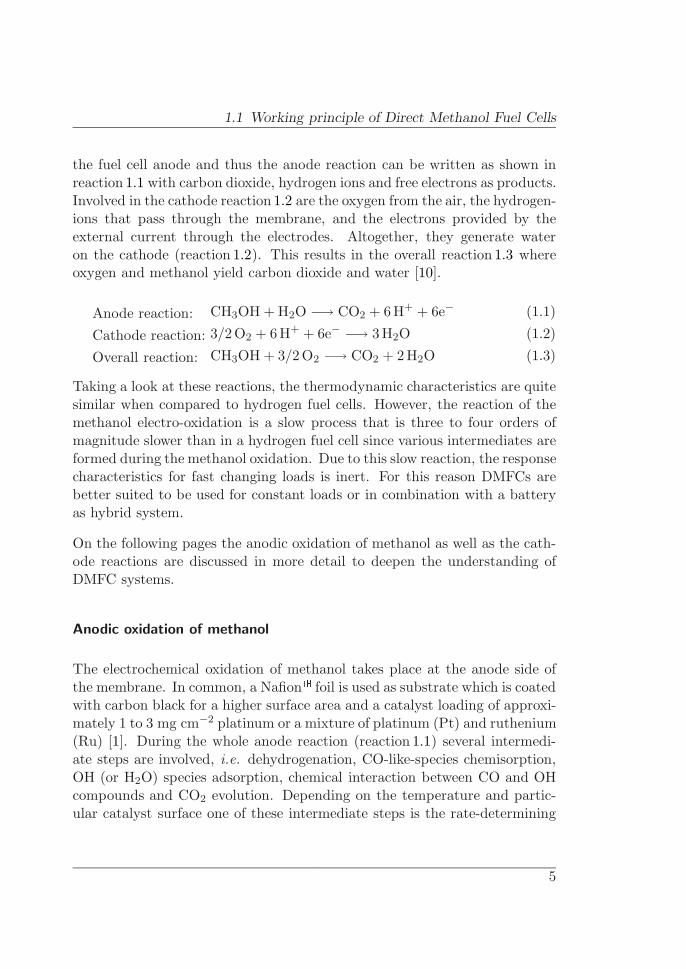
the fuel cell anode and thus the anode reaction can be written as shown inreaction 1.1 with carbon dioxide, hydrogen ions and free electrons as products.Involved in the cathode reaction 1.2 are the oxygen from the air, the hydrogen-ions that pass through the membrane, and the electrons provided by theexternal current through the electrodes. Altogether, they generate wateron the cathode (reaction 1.2). This results in the overall reaction 1.3 whereoxygen and methanol yield carbon dioxide and water [10].
Anode reaction:Cathode reaction:Overall reaction:
CH3OH + H2O −→ CO2 + 6H+ + 6e−
3/2O2 + 6H+ + 6e− −→ 3H2OCH3OH + 3/2O2 −→ CO2 + 2H2O
(1.1)(1.2)(1.3)
Taking a look at these reactions, the thermodynamic characteristics are quitesimilar when compared to hydrogen fuel cells. However, the reaction of themethanol electro-oxidation is a slow process that is three to four orders ofmagnitude slower than in a hydrogen fuel cell since various intermediates areformed during the methanol oxidation. Due to this slow reaction, the responsecharacteristics for fast changing loads is inert. For this reason DMFCs arebetter suited to be used for constant loads or in combination with a batteryas hybrid system.
On the following pages the anodic oxidation of methanol as well as the cath-ode reactions are discussed in more detail to deepen the understanding ofDMFC systems.
Anodic oxidation of methanol
The electrochemical oxidation of methanol takes place at the anode side ofthe membrane. In common, a Nafion� foil is used as substrate which is coatedwith carbon black for a higher surface area and a catalyst loading of approxi-mately 1 to 3 mg cm−2 platinum or a mixture of platinum (Pt) and ruthenium(Ru) [1]. During the whole anode reaction (reaction 1.1) several intermedi-ate steps are involved, i.e. dehydrogenation, CO-like-species chemisorption,OH (or H2O) species adsorption, chemical interaction between CO and OHcompounds and CO2 evolution. Depending on the temperature and partic-ular catalyst surface one of these intermediate steps is the rate-determining
5

1 Introduction
step (rds). A combination of several methods to analyse the anode reactionrevealed that the electro-oxidation of the methanol on Pt-based catalysts pro-ceeds through the mechanism which is a sequence of non-elementary reactionsteps as described below [10]:
CH3OH + 3Pt −→ Pt3−COH (1.4)Pt3COH −→ Pt−CO + H+ + 2Pt (1.5)Pt + H2O −→ Pt−OH + H+ + 1e− (1.6)Pt−OH + Pt−CO −→ 2Pt + CO2 (1.7)
In case of a catalyst plating with platinum and ruthenium the catalyticactivity and thus the methanol reaction can be increased, dependent on theworking temperature of the fuel cell and the amount of ruthenium. Theruthenium is involved in two reaction steps: First, water discharging occursat the ruthenium sites, resulting in the formation of Ru-OH groups and thusreaction 1.6 is substituted by the reaction 1.8. Second, the final reaction 1.7is changed to reaction 1.9 where the Ru-OH groups with the neighbouringmethanolic residues are adsorbed to give carbon dioxide [10].
Ru + H2O −→ Ru−OH + H+ + 1e− (1.8)Ru−OH + Pt−CO −→ Ru + Pt + CO2 + H+ + 1e− (1.9)
Due to the better performance, a membrane with a platinum-ruthenium cat-alyst loading is used in this work.
Cathodic reduction of oxygen
On the cathode side of low temperature fuel cells the most widely used elec-trocatalysts are based on platinum due to their intrinsic activity and stabilityin acidic solutions. Nevertheless there is still great interest in the develop-ment of more active, selective and inexpensive electrocatalysts for oxygenreduction.
6

1.1 Working principle of Direct Methanol Fuel Cells
There are only limited options to investigate in to reduce costs and improvethe electrocatalytic activity of platinum. This is based on the fact that thecathode catalytst is the same as on the anode and for the proton conductivitythe membrane has to take up water. In addition to the water, methanolis taken up and crosses through the membrane to the catalyst sites at thecathode and reacts to CO2 and H2O there. This phenomenon is denoted asmethanol cross-over, a parasitic effect that leads to significant losses.
Nafion�, the most common membrane material, is a sulfonated tetrafluo-roethylene based fluoropolymer-copolymer that rapidly transports methanol.This yields methanol reactions on the cathode and thus a significant currentloss of 10% to 20% [10]. The cross-over is influenced by membrane character-istics, membrane temperature and the operating current density [11, 12]. Anincrease in temperature yields an increase of the methanol diffusion coefficientand a further swelling of the membrane, leading to a higher cross-over. In-cluded in the cross-over are both, the methanol permeability due to a gradientin methanol concentration and molecular transport caused by electro-osmoticdrag. As the current membranes have to take up water and the methanolcross-over can not be avoided the objective is to identify methanol tolerantcatalyst alternatives to platinum for the oxygen reduction. An alternative forplatinum could have the disadvantage that the permeated methanol wouldnot be oxidized at the cathode surface to CO2 and thus contaminate the wa-ter at the cathode side, which could cause environmental problems. However,the great advantage would be the enhanced oxygen reduction since methanoloxidation and oxygen reduction compete for the same catalytic sites andin addition the methanol oxidation yields a mixed potential at the cathodewhich reduces the cell open circuit voltage.
To clarify that the methanol and the oxygen do compete for the same sites,the potential reaction mechanisms for the oxygen reduction and the methanoloxidation at the cathode are shown next [10].
Oxygen reduction:
O2 + Pt −→ Pt−O2 (1.10)Pt−O2 + H+ + 1e− −→ Pt−HO2 (1.11)Pt−HO2 + Pt −→ Pt−OH + Pt−O (1.12)Pt−OH + Pt−O + 3H+ + 3e− −→ 2Pt + 2H2O (1.13)
7

1 Introduction
Since it has been observed that the platinum particle size and orientationaffects the activity of the particle and thus the reaction rate, it can be con-cluded that the dual site reaction 1.12 represents the rate determining stepduring the oxygen reduction [10].
The parasitic methanol oxidation corresponds with the anode reactions 1.4to 1.7. For the methanol oxidation at the cathode, the methanol chemisorp-tion will be favoured by three neighbouring platinum sites that occupy theproper crystallographic arrangement. At high cathodic potentials the waterdischarging reaction (reaction 1.6) is largely favoured and thus oxidation ofthe methanolic residues adsorbed on the surface proceeds quickly, producinga parasitic anodic current on the cathode electrode, which generates extraheat [10, 13].
Conclusion
Concluding the investigation of the working principle of DMFCs, the mostbasic reactions have been explained and should be considered during the de-velopment of a DMFC system for both, the anode and the cathode side. Atthe anode side of the membrane a mixed catalyst plating with platinum andruthenium should be used. Furthermore during the reaction of the methanol,the product CO2 typically forms gas bubbles that block parts of the mem-brane and thus catalyst sites. These bubbles have to be removed from themembrane surface either by using active peripherals or passively like stud-ied in this work. On the cathode side, however, the methanol cross-over,that yields parasitic methanol reaction and thus loss of electrical power, hasto be minimized by finding the optimum between membrane thickness andmethanol concentration.
8

1.2 State-of-the-art in µDMFC development
1.2 State-of-the-art in µDMFC development
Presently there exists a large variety of possible µDMFC architectures. Ingeneral they vary in terms of:
� fuel supply methods
� complete system assembly
� layout of a single cell or fuel cell stack
� layout of the single flow field
All of these four can be freely combined. Besides the large variety of fuelcell setups all have to deal with the same problems that can be more or lesssevere, depending on the system design. These issues are discussed in thefollowing.
System design: fuel supply
The architecture of a µDMFC does not only have to meet particular ap-plication requirements such as a compact size and ease of handling. It hasto ensure the desired performance, reliability and moderate fabrication costs.The system architecture as considered here includes the fuel cell and all addi-tional components to ensure reactant supply and to deliver a required poweroutput. One can classify the system architectures into two main categories:active and passive µDMFC systems [13, 14].
Active systems are using extra components, electrically supplied by the fuelcell, such as pumps for methanol supply or fans for cooling, humidification,reactant and product control. The additional components, although using apart of the energy provided by the fuel cell, allow for operating the system atfavourable conditions in terms of temperature, pressure, reactant concentra-tion and flow rate. In general, the active systems are better suited for largerfuel cell systems where additional costs and greater system complexity areaffordable.
9
1 Introduction
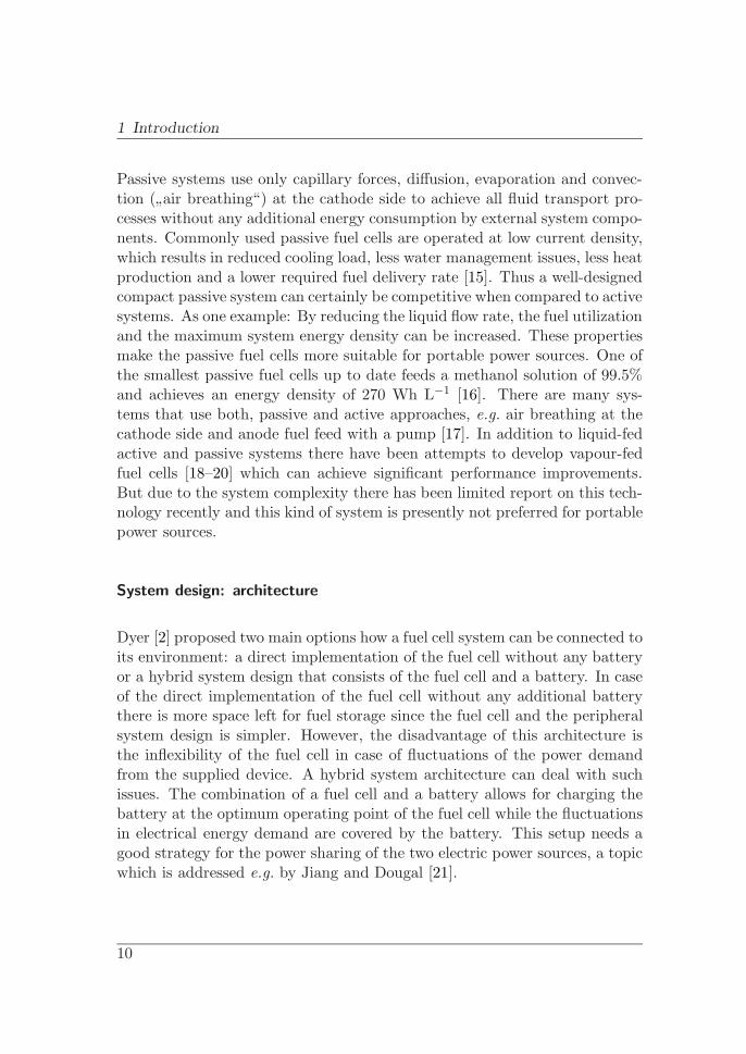
Passive systems use only capillary forces, diffusion, evaporation and convec-tion (”air breathing“) at the cathode side to achieve all fluid transport pro-cesses without any additional energy consumption by external system compo-nents. Commonly used passive fuel cells are operated at low current density,which results in reduced cooling load, less water management issues, less heatproduction and a lower required fuel delivery rate [15]. Thus a well-designedcompact passive system can certainly be competitive when compared to activesystems. As one example: By reducing the liquid flow rate, the fuel utilizationand the maximum system energy density can be increased. These propertiesmake the passive fuel cells more suitable for portable power sources. One ofthe smallest passive fuel cells up to date feeds a methanol solution of 99.5%and achieves an energy density of 270 Wh L−1 [16]. There are many sys-tems that use both, passive and active approaches, e.g. air breathing at thecathode side and anode fuel feed with a pump [17]. In addition to liquid-fedactive and passive systems there have been attempts to develop vapour-fedfuel cells [18–20] which can achieve significant performance improvements.But due to the system complexity there has been limited report on this tech-nology recently and this kind of system is presently not preferred for portablepower sources.
System design: architecture
Dyer [2] proposed two main options how a fuel cell system can be connected toits environment: a direct implementation of the fuel cell without any batteryor a hybrid system design that consists of the fuel cell and a battery. In caseof the direct implementation of the fuel cell without any additional batterythere is more space left for fuel storage since the fuel cell and the peripheralsystem design is simpler. However, the disadvantage of this architecture isthe inflexibility of the fuel cell in case of fluctuations of the power demandfrom the supplied device. A hybrid system architecture can deal with suchissues. The combination of a fuel cell and a battery allows for charging thebattery at the optimum operating point of the fuel cell while the fluctuationsin electrical energy demand are covered by the battery. This setup needs agood strategy for the power sharing of the two electric power sources, a topicwhich is addressed e.g. by Jiang and Dougal [21].
10

1.2 State-of-the-art in µDMFC development
Unit cell and stack architecture
For the fuel cell itself one has to distinguish between the unit cell and theassembly of multiple cells to a stack. The unit cell can be set up in threedifferent configurations [13, 22]. A so called unit single cell is the most simpledesign that consists of a cathode current collector where the oxidant is deliv-ered, a diffusion layer, a membrane coated on both sides with the catalysts,also named membrane electrode assembly (MEA), a second diffusion layerand the anode current collector with the implemented flow field for methanolfeed. This configuration is depicted in figure 1.3(a) and is the classical fuelcell setup, where the fuel/oxidant delivery is separated and avoids that thefuel and oxidant can come into contact before the reaction.
(a) (b) (c)
MEA cathode
anode air
air
air
methanol
membrane catalyst
diffusionlayer
Figure 1.3: Three basic fuel cell designs: unit single cell (a), unit bi-cell (b)and planar cell (c) [13, 22]
In the second configuration, the unit bi-cell, the reactants are also separatedbut in this arrangement, shown in figure 1.3(b), two unit single cells are shar-ing the central anode current collector and the fuel feed. The anode layeris sandwiched in-between the diffusion layers, the MEAs and the cathodecurrent collectors.
The third possible configuration is called planar design since all feed channels(fuel and oxidant) are located at the same side of a substrate that has to bean insulator. The feed channels are interdigitated (see figure 1.3(c)) so thatthe reaction can occur between them. Placed on top of the substrate is thediffusion layer, the MEA and finally the interdigitated anode and cathodecurrent collectors. This allows for a monolithic integration especially in very
11
1 Introduction
small chip-based systems. The drawback of this two dimensional configura-tion is the large surface area that is required to achieve the same performanceas the other two setups.
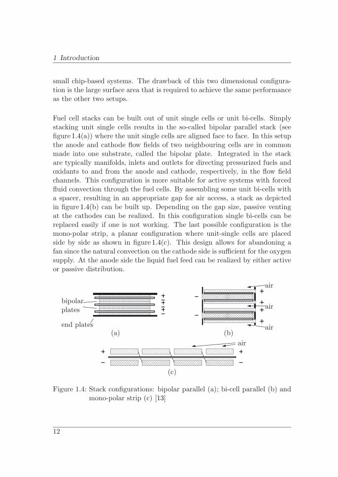
Fuel cell stacks can be built out of unit single cells or unit bi-cells. Simplystacking unit single cells results in the so-called bipolar parallel stack (seefigure 1.4(a)) where the unit single cells are aligned face to face. In this setupthe anode and cathode flow fields of two neighbouring cells are in commonmade into one substrate, called the bipolar plate. Integrated in the stackare typically manifolds, inlets and outlets for directing pressurized fuels andoxidants to and from the anode and cathode, respectively, in the flow fieldchannels. This configuration is more suitable for active systems with forcedfluid convection through the fuel cells. By assembling some unit bi-cells witha spacer, resulting in an appropriate gap for air access, a stack as depictedin figure 1.4(b) can be built up. Depending on the gap size, passive ventingat the cathodes can be realized. In this configuration single bi-cells can bereplaced easily if one is not working. The last possible configuration is themono-polar strip, a planar configuration where unit-single cells are placedside by side as shown in figure 1.4(c). This design allows for abandoning afan since the natural convection on the cathode side is sufficient for the oxygensupply. At the anode side the liquid fuel feed can be realized by either activeor passive distribution.
(a) (b)
(c)
air
air
air
air
end plates
bipolarplates
Figure 1.4: Stack configurations: bipolar parallel (a); bi-cell parallel (b) andmono-polar strip (c) [13]
12

1.2 State-of-the-art in µDMFC development
Flow field layout
As mentioned before the anode as well as the cathode are structured to supplythe fuel cell with fuel and oxidant. The oxidant, usually air, can be deliveredby pumps, fans or compressors or driven by natural convection only, called selfbreathing. For small portable systems it is preferred to use a self breathingconfiguration and renounce external accessories. In this case the flow fielddesign is usually kept simple and the cathode substrate has slots, round orsquare holes and no distinct flow field channels [22–24].
The situation at the anode side is somewhat different: on the one hand thefuel has to be delivered to the fuel cell but at the same time the gas bubbles,formed during the methanol reaction, have to be removed. In literature sev-eral different designs can be found like shown in figure 1.5. The designs rangefrom direct supply, pillar like structures, parallel and serpentine structuresto interdigitated structures.
(a) (b) (c) (d)
(e) (f) (g) (h)
Figure 1.5: Typical flow field designs according to [22]:(a) direct supply, (b) distribution pillars,(c) parallel channels, (d) serpentine chan-nels, (e) parallel/serpentine channels, (f) spi-ral channel, (g) interdigitated channel, (h) spi-ral/interdigitated channels
The first fuel supply design waives channels, but to ensure electrical con-tact and increase pressure a conducting layer like a metal foam is required
13

1 Introduction
[25] which can be used for a diffusion based methanol supply through theporous media [26–28]. A flow field with conducting pillars, also called pinor grid design, yields a little pressure drop for the fuel feed but the sharpedges may damage the membrane already at little contact pressures. In ad-dition the low contact pressure on the membrane leads to a higher electricalcontact resistance. One of the most prominent designs is the parallel de-sign (cf. figure 1.5(c)) [22, 23, 29–32] which reduces the supplying pressureand at the same time decreases the mean fuel velocity sufficiently by keepingan almost homogeneous flow in all the channels. The lower velocity yieldsa longer fuel residence time and thus a higher fuel utilization. The secondvery popular design is the serpentine channel as shown in figure 1.5(d). Thechannel length and thus the pressure drop is increased in this design forcingthe methanol into the diffusion layer and leading to a better fuel perme-ability and system performance. In addition, developing gas bubbles areforced downstream toward the outlet of the fuel cell by the single channel de-sign. As a negative consequence a non-uniform current density distributionappears since the methanol concentration decreases with the channel length[33]. To reduce the non-uniform current density distribution and the pressuredrop along the channel a combination of parallel and serpentine structures(figure 1.5(e)) is sometimes used [34, 35]. A spiral design [36] has the sameadvantage as the serpentine design but keeps the area with the lower fuel con-centration, the channels end, closer to the channel inlet with the higher fuelconcentration. Finally there exist interdigit designs as shown in figure 1.5(g)and (h) where the inlet and outlet channel are separated, i.e. the inlet chan-nel has a dead end design. The methanol is forced through the diffusion layertoward the outlet channel. The interdigit design exhibits the highest pressuredrop and the fuel is almost depleted when flowing through the exit side. Theadvantages and disadvantages of the flow field designs discussed above aresummarized in table 1.1 together with some references for their applicationin active and passive fuel cell architectures.
14

1.2 State-of-the-art in µDMFC development
Table 1.1: Flow field designs used in µDMFCs according to [13]
Flow fieldlayout
Advantages Disadvantages DMFCliterature
Straight(parallel)
Lower pressure drop Prone to inhomoge-neous reactant dis-tribution and prod-uct removal
Active[37–40]Passive [41]
Serpentine(meander)
Helpful to removegas product at theanode and water atthe cathode, and toenhance two-phasemass transport
Higher pressuredropsMore peripheral en-ergy required
Active[38, 42–44]
Spot (pinor grid)
Similar to straightflow fields as above
Similar to straightflow fields as above
Active [44]
Inter-digitated
Enhanced local masstransport by bothdiffusion and forcedconvection
High-pressure differ-ence between chan-nels requiredHigh peripheral en-ergy required
Active[44, 45]
Porousmediadiffusion
Simple, low cost andcompact
Lower mass transferrates dependent onporous mediaSeparate current col-lector needed
Passive[26–28]
15

1 Introduction
Common issues
Apart from the architecture of the fuel cell there are further topics discussedin literature regarding single parts of the fuel cell and the reaction process.The four most prominent topics are the membrane and the cross-over throughit (1), the water management at the cathode (2), the reaction temperature(3) as well as the reaction product CO2 as gas bubbles in the cathode liquidphase (4).
The membrane and its coating is one of the most important topics since thisis the central element of the fuel cell. On the one hand the membrane hasto swell and saturate with water for a better proton transport, on the otherhand methanol transport through the membrane has to be reduced or, inthe ideal case, should be eliminated. To reduce cross-over, the methanolconcentrations used at the membrane are usually low. According to thereview article of Nguyen and Chan [22] the methanol concentrations used incommon are in the range of 0.5M to 6.0M.
Water management is another important aspect for the fuel cell develop-ment since the membrane relies on proton transport and a too high waterproduction rate can cause flooding of the cathode side and reduce the fuelcell’s efficiency to take up oxygen. To gain a higher energy density a highermethanol concentration is preferred but this also leads to increased cross-over[10]. For this reason a water control is necessary that prevents flooding andtransfers water from the cathode to the anode side to dilute the methanol.However, in small systems an active water control is not feasible and passivewater transport is the more likely solution, since water can diffuse from theanode to the cathode side.
The temperature also plays an important role since it influences the systemperformance in various ways. Vapour pressure at the cathode and anode aswell as the reaction kinetics depend on the temperature. If the temperatureis too high, the evaporation is accelerated and the membrane dries out in ad-dition to a higher methanol cross-over, resulting in a lower system efficiency.When the temperature is too low, water droplets form at the cathode sidedue to the low evaporation rate and the fuel cell can be flooded. Furthermore,at low temperatures the membrane conductivity is reduced. Thus water and
16

1.3 Aim and structure of the thesis
temperature management are inter-related. Though temperature control isnecessary for a stable operation, an active system architecture with temper-ature control and heating elements is required. Due to the demand of activeelements it is difficult to implement this in small portable fuel cell systems[13, 15].
The CO2 bubbles are formed at the anode side of the fuel cell since the CO2 isonly partially dissolved in the methanol solution. These gas bubbles consistof CO2, water and methanol vapour and block parts of the membrane area.Therefore, the gas bubbles have to be removed from the system.
1.3 Aim and structure of the thesis
Aim of the present work is the development of a passive micro direct methanolfuel cell with a stable operation over a long time. The key issue that has tobe solved to enable passive operation is the fluid management at the anodeside of the fuel cell. Starting from an active fuel cell system design, thesystem is transformed into a fully passive system where the methanol solutionis recirculated by using the CO2 gas bubbles which are removed from themembrane area due to capillary forces.
While this first chapter was used to introduce the basic working principleand typical architectures for µDMFCs, the remaining chapters deal with thedevelopment of the passive system. As basic system, the unit single cell(cf. figure 1.3) has been identified as best architecture to develop an experi-mental fuel cell that can easily be operated in an active and passive experi-mental setup.
A theoretical evaluation how the system energy density can be increased bycombining different concepts for fuel supply (methanol feed) and waste (CO2
bubble) removal at the anode side is performed in Chapter 2. The state-of-the-art-system combines an active, continuously pumped fuel supply andCO2 removal. This system has the lowest system energy density since theperipherals are active all the time. Further combinations with increasingsystem energy density studied in this work are: discontinuous pumping ofmethanol with discontinuous pumped and capillary CO2 removal, capillary
17

1 Introduction
based fuel supply and CO2 removal and diffusion based fuel supply withcapillary CO2 removal. The combination of capillary based fuel supply andCO2 removal is based on the idea that the movement of gas bubbles in taperedchannel designs can be used to generate a liquid flow in the channels whichcan be used to recirculate the methanol solution within a suitable fuel cellassembly. To further increase the system energy density, a diffusion basedapproach for methanol supply combined with a passive gas bubble removal ispresented and an analytical model to determine the required design for thefuel cell setup is developed.
Chapter 3 describes the manufacturing of the fuel cell assembly, the experi-mental setups used in this thesis and the experiments with actively pumpedmethanol supply and CO2 removal. The reference values for all succeedingexperiments are determined by experiments with a state-of-the-art contin-uous pumped fuel supply. These reference experiments are performed withall flow field designs studied in this thesis. Furthermore, a first approach toincrease the system energy density is studied by activating the pump at in-tervals. With this approach the energy demand of the peripherals is reduced,since the fuel cell runs passively most of the time.
For tapered channels it is validated in Chapter 4 that the passively removedCO2 gas bubbles generate a high enough liquid flow rate to supply the fuelcell with fresh methanol. First, it is demonstrated that gas bubble movementwithin tapered structures can be simulated by CFD with reasonable accuracy.Second, the simulation of a single flow field channel plus reservoir shows thata liquid flow rate is generated which exceeds the minimum required methanolflow rate for passive fuel cell operation. These simulation results are comparedto experiments with single flow field channels and artificial bubble generationas well as to flow rates measured in fuel cell experiments.
Succeeding the validation that the generated liquid flow rate is high enough tosupport passive long term fuel cell operation, the corresponding experimentsare performed in Chapter 5. The experiments show a stable, passive longterm fuel cell operation of more than 15 hours at efficiencies of about 10%.A series of experiments is performed in order to find a correlation betweenthe amount of methanol supplied to the fuel cell and its runtime which canbe used for the system design. An approach to further reduce the size of a
18

1.3 Aim and structure of the thesis
passive system is performed by re-dosing pure methanol at intervals into asmall reservoir filled with methanol solution.
The different fuel cell setups and flow field designs explored in this thesis proofthat a fuel cell system with a stable and fully passive operation over severalhours can be realized. Based on these results and observations gatheredthroughout this work an improved fuel cell design is suggested in Chapter 6.
19


2 Concepts for passive fluid management
In the first chapter various system concepts for portable fuel cells as well asthe current research topics have been introduced in brief. The objective ofthis thesis is to study possible architectures for fluid management in µDMFCsystems. Therefore, the possible methods for the fuel supply and the carbondioxide removal have to be categorized first. After identifying the differentoptions, possible solutions will be studied. This is performed with focus onpassive system architectures. In this chapter an approach for passive gasbubble removal as well as diffusion based methanol supply will be discussed.
Table 2.1 shows the three main topics that have to be discussed: fuel supplywith methanol and oxygen and waste removal of CO2 for active and pas-sive µDMFC systems. Active systems can be considered as state-of-the-artsystems. Thus these approaches are not discussed in detail although someconcepts in this thesis belong to this category. Passive systems can still beconsidered as current research topics.
Table 2.1: Anode and cathode fluid management in µDMFC
Fuel supply CO2 degassing Oxygen supply
active state-of-the-art state-of-the-art state-of-the-arte.g. [36, 43]
passive current researchtopics
current researchtopics
state-of-the-arte.g. [26, 27]
21

2 Concepts for passive fluid management
2.1 Active versus passive fuel cell systems
The oxygen supply solutions for active and passive are state-of-the-art andthus they are not discussed furthermore. The methanol fuel supply and CO2
degassing can still be considered as one of the key items for the developmentof µDMFC systems for portable applications. There are two different fluidicunit operations at the anode side that can be considered separately as shownon the X and Y-axis of figure 2.1. Sub-dividing the two unit operations intothe four most discussed categories found in literature, active pumping contin-uously or discontinuously and passive by capillary forces or diffusion, yieldsa matrix with 16 combinations for fuel supply and CO2 degassing.
As shown in figure 2.1 some of the combinations do not have examples or alink to this work. These combinations are not applicable, although the fuelcell itself can be operated but the effects can not be separated. For exampleone of these combinations is the capillary methanol feed in combination withactive pumped CO2 removal. Since the amount of CO2 produced during fuelcell operation is above the saturation limit for CO2 in a water solution [47] gasbubbles grow and there is a two-phase regime in the flow field. Thus pumpingthe gas while only having passive liquid flow is logically not possible as theactive pumping of CO2 can not be decoupled from pumping methanol. Forthe other combinations indicated in light grey, similar explanatory statementscan be found why they are not applicable. The other sets of combinationsare briefly explained below and in more detail in later sections.
The first set of applicable options to discuss are those described as activesystems for fuel feed and bubble removal. By using a state-of-the-art activelyand continuously pumped [37, 38, 40, 42–45] or discontinuously operatedsystem [46], the gas bubbles are flushed out of the flow field during the time,the pump is activated. These approaches have previously been described asstate-of-the-art and are discussed in section 3.4. In these cases, the fuel feedand the CO2 degassing can not be decoupled and thus the combinations ofa continuous pumped fuel feed with discontinuous CO2 degassing and viceversa are not applicable.
Taking a look at the combination of an actively pumped fuel feed and passivegas bubble removal, possible solutions can be found for both types of active
22

2.1 Active versus passive fuel cell systems
CO
2de
gass
ing
(bub
ble
rem
oval
)
fuel supply (methanol feed)
pump(external,
continuous)
pump(external,
continuous)
pump(external,discontinu-
ous)
pump(external,discontinu-
ous)
capillary
capillary
diffusionbased
diffusionbased
section 3.4 section 3.4 section 5.2theoreticalmodel insection 2.4
section 3.4and
e.g. [46]
notconsidered
in thiswork
section 3.4and e.g.
[37, 38, 40,42–45]
notconsidered
in thiswork
pass
ive
passive
passive
active
active
active
mixed
mixed
Figure 2.1: Matrix with applicable ( ) and not applicable ( ) configurationsfor anode fuel feed and carbon dioxide removal. The dotted linesindicate the transition from active to passive system concepts.The text gives reference to literature or to work done within thisthesis.
23

2 Concepts for passive fluid management
pumping, continuous as well as discontinuous. For the two options of passivegas bubble removal, only the capillary method is possible. In a continuouslypumped fuel cell with very low flow rate the gas bubbles can be removedby capillary forces by appropriately designed flow field channels as discussedlater in section 3.4. The same can be realized for discontinuously pumpedfuel feed (see section 3.4). In this setup, the gas bubbles are flushed out ofthe flow field channels while the pump is activated and removed based oncapillary forces while the pump is inactive. To achieve this an appropriateflow field channel design is necessary.
The focus of this work is set on the last combination with passive fuel feedand passive CO2 removal. The CO2 removal by capillary forces is possible incombination with both options for passive fuel feed: capillary and diffusionbased. The combination of the capillary based fuel supply together with thecapillary removal of the CO2 gas bubbles is the most promising combinationfor a completely passive fuel cell setup and thus discussed in detail in thechapters 4 and 5. The second option by using a diffusion based methanolsupply is studied as model only in section 2.4 and not in the experimentalpart.
Although most of the architectures can be categorized by the matrix depictedin figure 2.1 some additional variants of passive cells with passive fuel feedand passive carbon dioxide removal are possible and discussed in literature[13]. In common they are based on a vertically oriented fuel cell where thebubbles are removed from the cell due to buoyancy [48]. Furthermore thereexist cells that recirculate the fuel due to buoyancy in a vertical fuel cell withserpentine flow field structure [49] or self-pressurization of the fuel reservoir[50].
Summarizing the last paragraphs yields that for passive supplied systemsone can distinguish between buoyancy/hydrostatic, capillary and diffusivesupplied fuel cell systems, depending on the dominating driving force theyare based on. All these passive systems have to ensure a self-sustaining supplyrate to prevent the fuel cell from starving. Furthermore, a sufficient degassingrate has to be guaranteed to prevent the active surface from being blockedby carbon dioxide gas bubbles.
24

2.2 Flow field design for passive systems
2.2 Flow field design for passive systems
From a technical point of view the methanol supply and CO2 removal can befurther split up as depicted in figure 2.2. Prior to the system design, one hasto decide whether a central or decentral supply and/or degassing is preferred.
CO2
methanol· · ·
...
centralsupply
decentralsupply
centraldegassing
decentraldegassing
fuelinlets
fuelinlets
CO2 /disposaloutlets
disposaloutlets
CO2
out-lets
Figure 2.2: Sketches of the different methods to supply (black arrows) a pas-sive fuel cell system and to remove the CO2 (gray arrows). Thefuel can be supplied via capillary forces or by diffusion througha membrane. Removal of the CO2 can be realized by capillarypumping or through a hydrophobic membrane. However the tran-sition between the different setups can be smooth.
A central supply is the commonly used approach of one or more dedicatedfeed channels, e.g. [41], while decentral supply is characterized by supplyingthe membrane evenly over the complete area as done for example by Kimet al [27]. The same differentiation can be done with respect to the CO2
removal. Examples for these system designs are:
� Liu et al [41] (central MeOH, central CO2)
� Meng et al [51](central MeOH, decentral CO2)
25

2 Concepts for passive fluid management
� Guo and Cao [48] (decentral MeOH, central CO2)
� Kim et al [27] (decentral MeOH, decentral CO2)
The decentral design approach with an ubiquitous fuel supply and carbondioxide removal yields the need for membrane technologies that allow gastransfer and methanol diffusion as well as providing the necessary electricalcontact and contact pressure to the membrane. The central approaches arefavourable, since they allow an easy integration of the fuel cell system.
Conclusion
Amongst the wide field of possible system designs that exist and have beendiscussed in this section the central approach for the fuel supply and CO2
removal yields the benefits of high flexibility in terms of system design andmanufacturing technology of the parts. Thus this concept has been chosenfor the system studied in this thesis.
2.3 Concepts for gas bubble removal based on capillary forces
Other than in an active system where the CO2 is flushed out, in a passivesystem buoyancy [48, 49] or capillary forces can be used to separate thecarbon dioxide from the methanol solution [51, 52]. The approach of Menget al [53] is based on hydrophobic holes that are etched in the backplate ofthe anode flow field and directly remove the bubbles from the fuel cell in adecentral way.
Another approach is to use a flow field design, that forces the gas bubblesto move away from the active area. To achieve this, first a channel designhas to be found that shapes the gas bubbles due to the channel geometry,enhances bubble mobility and allows to control the ratio between bubblesand methanol coverage on the active surface. The T-shaped channel designas shown in the publications of Kohnle et al [54], Waibel et al [55] andLitterst et al [56, 57] meets the requirements mentioned above. Figure 2.3depicts the three different bubble shapes that can be achieved in a T-shaped
26

2.3 Concepts for gas bubble removal based on capillary forces
(a) (b) (c)
liquid gas bubble
Figure 2.3: Gas bubble positions in a T-shaped micro-channel design as topand cross-sectional view: (a) vertical, (b) blocking and (c) hori-zontal [56, 57]
channel design: vertical, blocking and horizontal. However, in this design agas bubble is only moving due to buoyancy if the channel is inclined oriented.
To achieve a bubble movement in a horizontal oriented channel, the bubblescan be forced to move by tapering the channel along its length axis. Sucha tapered channel design generates a non-uniform capillary pressure alongthe gas bubble’s length as sketched in figure 2.4. This is due to the differentcurvatures r an elongated gas bubble exhibits at its distant ends in a taperedchannel. Since the capillary pressure Pcap is a function of r, an elongatedbubble in a tapered channel has different capillary pressures at the distantends resulting in a force that moves the bubble towards the wider channelpart in case of small contact angles (Θ � 90�). The movement �v of the bubbleproceeds until the capillary pressures are in equilibrium, e.g. a spherical cross-section along the tapered channel is attained.
(a) (b) (c)
Pcap,1(r1) � Pcap,2(r2) Pcap,1(r1) > Pcap,2(r2) Pcap,1(r1) = Pcap,2(r2)
�v � 0 �v > 0 �v = 0
Figure 2.4: Two-dimensional sketch of gas bubble movement in a taperedchannel driven by capillary pressures (a) and (b). Equilibriumstate with no bubble movement (c).
27

2 Concepts for passive fluid management
In total four different channel types as shown in table 2.2 have been consideredin this work. The different channel geometries are denoted as R-type, A-type,B-type and C -type channels. The channels are arranged in a parallel channellayout, since this flow field design can be used for active and passive systems.
Table 2.2: Classification of the different studied channel geometries with theMEA always placed the bottom side of the channel
Type Sketch Description
R
h
wl
Reference geometry as astraight channel without anytapering angles
A α
h
wl
Straight channel geometrytapered along its length axis
B α
β
h wl
H
W T-shaped channel geometrytapered along its axis and sym-metrically at its cross-section
C α
h
wl
Planar channel geometrytapered along its cross-section.
The R-type channel is used as reference in all simulations and experiments,discussed in the following chapters. It has been chosen as reference due to tworeasons: First, this kind of channel is a standard channel geometry used inmost µDMFC-systems throughout literature and second, the R-type channelis expected to exhibit no capillary driven gas bubble movement.
In an A-type channel that is tapered along its length axis, the growing gasbubbles will expand over the whole cross-section of the channel and start
28

2.3 Concepts for gas bubble removal based on capillary forces
to move towards the wider channel part. The tapered geometry alreadyintroduces a preferred direction of the bubble movement.
The B-type channel has a T-shaped cross section and is tapered along itslength axis as well as symmetrically at its cross-section. It is expected that agas bubble that starts to grow in the side arms of the T-shape moves towardsthe central channel first. The channel layout is chosen according to theinitial idea of a T-shaped channel for improved bubble mobility presentedin [17] and designed based on the design rules presented in [57] to resultin a vertical bubble position (cf. figure 2.3(a)). The gas bubble will attendthis position once it reaches the middle channel and move to the end ofthe channel if the bubble size is large enough. This channel layout providesblockage of the whole channel cross-section and implies an intrinsic passivemechanism to transport and guide a gas bubble out of the system as describedin the patent application ”Device comprising a channel carrying a mediumand method for removing inclusions“ [58]. Furthermore, the vertical bubbleorientation provides the least coverage of the active surface by gas bubblesas the majority of the gas bubbles are located in the central channel, whilethe side channels remain almost free of bubbles.
The third tapered design (C -type), tapered along its cross-section, is expectedto yield a bubble movement towards the wider part of the cross-section. Al-though these channels have been manufactured, the first fuel cells experi-ments proofed that this channel type does not work, neither in an active norin a passive setup. Reasons for the malfunction of this channel type is theswelling of the membrane, reducing the channel height and the gas bubbleswhich completely block the flow field and do not move out of the channel.
First, a B-type channel has been manufactured as shown in [59] and com-putational fluid dynamics (CFD) simulations of this channel type have beenperformed to show the capillary pressure based removal of gas bubbles. Inthe simulation a typical gas flow rate based on the estimation that a typicalcurrent density of j = 100mA cm−2 generates 0.26mL min−1 cm−2 of carbondioxide has been used. This gas flow rate φCO2 can be calculated by
φCO2 =j Vm,MeOH 60
eNA ne, (2.1)
29

2 Concepts for passive fluid management
where the current density/fuel cell load j and the molecular volume of meth-anol Vm,MeOH are divided by the elementary charge e, Avogadros constantNA and the number of electrons ne. Since it can be assumed that the bubblesdevelop randomly or at some distributed spots at the MEA a method thatmimics the same behaviour has been used. During the simulation time theboundary conditions at the MEA of the simulation model have been switchedrandomly after every 0.5 s for 10 out of 1000 small MEA areas from wall toinlet boundary and vice versa [17]. At the inlet boundaries, the mass flowrate φCO2 (equation 2.1) has been applied. However, to ensure gas bubbledevelopment and to keep the simulation time low, the gas flow rate wasincreased artificially by a factor of 1000. To keep the simulation comparableto the real system, the pulse where the inlet is active has been shortenedaccordingly to keep the overall flow rate comparable to the real fuel cellsystem. Thus it is ensured that the gas bubbles develop within reasonablesimulation time and the qualitative bubble behaviour in the flow field channelcan be studied which is the objective of the simulation. To further decreasethe simulation time the symmetry of the problem has been used as depictedin the first picture of figure 2.5. The inlet area is placed between two wallboundary surfaces to avoid non-physical effects due to gas bubbles cominginto contact with one of the outlets placed at the ends of the channel. Sucha contact would cause the bubble to be sucked out of the simulation domain.All these actions yield simulation times of several days, which is typical forsimulations with free surfaces as described more detailed in chapter 4.
The result of this simulation exhibits the anticipated bubble behaviour asdisplayed in figure 2.5. The bubbles grow randomly in the channel and oncethey touch the upper wall they start to move towards the central channel partof the channel due to the difference in the capillary pressures at the distantends of the bubble. On their way they wipe off other bubbles and merge withthem. Once the bubble has grown to a sufficient size in the central channel,where it adopts a vertical position, the bubble starts to move towards theoutlet of the channel. Thus the simulation shows that passive bubble removalin this type of double tapered channels is possible and that this mechanismis independent of the position where the bubble is growing.
30

2.3 Concepts for gas bubble removal based on capillary forces
symmetry
random inlets
t = 0.0ms t = 0.5ms t = 1.0ms
t = 1.25ms t = 1.5ms t = 1.75ms
Figure 2.5: Simulation of distributed gas bubbles in type B-channels as pre-sented in [17]
Conclusion
Although, in this section it has been shown by simulation that a passive bub-ble removal in a type B-channel, it still has to be determined which channeltype R, A, B or C yields the most suitable bubble removal for µDMFCs.Furthermore the bubble movement can induce a convective flow inside thechannel that has not been studied before. In addition to this convective flowinside the channel an overall flow along the channel is supposed to be gener-ated by the moving bubbles. This yields a passive pumping of liquid fuel intothe fuel cell and it has to be determined if this pumping method is sufficientfor a self sustaining fuel supply based on capillary forces only. This topic willbe further discussed in chapter 4.
31

2 Concepts for passive fluid management
2.4 Diffusion driven concepts for fuel supply
There have been several attempts to realize totally passive direct methanolfuel cells systems, as for example published by McLean [15], Toshiba Corpo-ration [16] and Guo and Cao [48]. If the system should be totally passive,one can only use the natural capillary forces as discussed above, convection(air breathing and methanol), evaporation (methanol) and finally diffusion.As addressed in section 1.2 a passive, diffusion based system has some smartadvantages compared to active systems.
To achieve a well designed diffusion based system, one has to know the factorsinfluencing the fuel cell performance. For this reason a 2-dimensional modelto study the most important geometrical parameters can be set up for a designas sketched in figure 2.6. A well defined diffusion distance d between themethanol source and the membrane has to be determined to gain a balancebetween fuel supply and methanol conversion that provides the optimummethanol concentration for the fuel cell system right at the MEA. On the onehand it must be secured that during the fuel cell operation the concentrationdoes not drop to much and no energy output is generated. On the otherhand, the concentration should not be too high, since the methanol crossoverthrough the membrane should be minimized.
methanol water/methanol-solution
CMeOH(d, t)
MEA
Figure 2.6: Model for a passive, diffusion based directmethanol fuel cell system with dilution of thehigh concentrated methanol due to diffusion(not to scale)
32

2.4 Diffusion driven concepts for fuel supply
The parameters influencing the passive, diffusion based fuel delivery are givenin table 2.3. These parameters can be used to determine the size of methanolfeed holes with methanol feed concentration Ca out of an infinite sourceat a given distance d to the membrane. The methanol concentration at agiven distance between source and drain can then be determined by using thediffusion equation. The analytical approach is based on a one-dimensional,stationary diffusion model with a point source and a drain in the distanced (cf. figure 2.7(a)). In the model the source is approximated by the cross-sectional area a = π r2 of the drill and the drain which is the area A ofthe membrane that has to be fed with methanol at a concentration CA. Themembrane area is approximated by a calotte of the size A = 2 π d2. Thus apoint source is imaged on the target area, modelled as calotte.
(a) (b)
A = 2π d2
a = π r2
dd
2 r
cover layerwith sources
2 d
MEA
Figure 2.7: (a) Draft used for the analytical approachto determine the necessary source area toachieve the necessary methanol concentrationof e.g. 2mol at a given source-drain spacing d.(b) Resulting system layout for the calculatedvalues of d = 100µm and r = 49.1µm
33

2 Concepts for passive fluid management
Table 2.3: Parameters of the analytical approach to determine the layout ofa passive, diffusion-based fuel cell system with exemplary values.
Symbol Value Alternative Descriptionvalue
d 100µm Distance between source andmembrane as well as the halfdistance between the sourceholes
A Membrane area to be pro-vided with methanol
a Source area
CA 2mol 1.224 1021 MeOHcm3 Target concentration at the
membrane
Ca 100 % 1.483 1022 MeOHcm3 Methanol concentration at
the infinite source
η 10 % Efficiency of the fuel cell
j 0.1 Acm2 Current density in the fuel
cell
T 300K Operation temperature
D 17.83 10−6 cm2
s Diffusion constantof methanol in liq-uid [60]; DMeOH
l =10−5.4163−999.778/T m2 s−1
Φ MeOHcm2 s
Methanol consumption
ne 6 e−MeOH Number of available elec-
trons per methanol molecule
∆C MeOHcm2 Concentration difference
r Radius of the source hole
34

2.4 Diffusion driven concepts for fuel supply
The diffusion equation 2.2 can be solved with the target area A, the methanolconsumption rate Φ, the diffusion constant of methanol at temperature T =300K of DMeOH = 17.83 10−6 cm2 s−1 and the concentration difference ∆Cbetween source and drain.
A Φ = D ∆C (2.2)
The methanol consumption rate Φ (equation 2.3) can be determined by thecurrent density j in the fuel cell, its efficiency η and the number of avail-able electrons per methanol molecule ne. The concentration difference ∆C(equation 2.4) can be described as a function of the source area a withmethanol concentration Ca and the drain area A with target concentrationCA scaling with the distance d (cf. figure 2.7(a)).
Φ =j
η ne(2.3)
∆C =a Ca − A CA
d(2.4)
By using the methanol consumption Φ (equation 2.3) and the concentrationdifference ∆C (equation 2.4) and applying it to the diffusion equation 2.2, theequation yields:
A j
η ne= D
a Ca − A CA
d(2.5)
Scaling equation 2.5 now by the area of the point source a = π r2 and thecalotte shaped drain A = 2 π d2 the radius r of the source yields:
r =√
2
√CA d2 D + d2 Φ√
Ca D(2.6)
Using the exemplary values given in table 2.3 a radius of r = 49.1µm canbe calculated that yields a constant diffusion based supply for a layout assketched in figure 2.7(b). Such a layout can be realized e.g. by using a per-forated steel plate with the given dimensions, porous structure or by drillingthe holes into the planar flow fields like type C (cf. table 2.2).
35

2 Concepts for passive fluid management
Conclusion
Although the hole array can be manufactured with given dimensions, therealization of a working fuel cell with this kind of setup is still not likely.This is due to the membrane swelling of unmodified Nafion� membraneswhich typically have a methanol uptake of ∼60wt% and a swelling ratio of 1.8[61]. The membrane swelling yields an even thinner spacing between the highconcentration methanol source and the membrane itself. Thus the distance dis reduced by a non-controllable amount and the membrane tends to curl dueto the swelling, making a well designed system setup very difficult. To reducethe curling of the membrane a very thin and stiff gas diffusion layer could beused, accepting a further reduction of the free channel space. Furthermorethe small spacing d yields that a growing CO2 gas bubble rapidly coversthe complete membrane area. To remove a gas bubble occupying the wholechannel is not easy to realize, especially with a non-controllable membranesurface. To overcome this problem a combination of the approach discussedabove and the degassing method proposed by Meng et al [52] seems to betheoretically favourable. From a technical point of view this is not feasiblewithout major difficulties. Therefore this approach is not further studied anymore during this work, although the type C flow fields dedicated for this kindof fuel cell setup have been designed and manufactured.
36

3 Experimental setup and reference fuel cell
In this chapter a description of the manufacturing and assembly process ofthe test cell for optical characterization and the fuel cell used for electricalexperiments within this work is given. First, the fabrication of the flow fieldswith type R, A and B-channels is explained. Second, the complete fuel cellassembly process which includes the assembly of the core layer consisting ofthe membrane, the gas diffusion layers and the PDMS sealing is discussed.Finally, the differences of the assembly process for test cells to study bubbleinduced pumping as used in chapter 4 are explained.
Afterwards, the active system setup will be characterized experimentally,since common fuel cells are active, continuously pumped systems. Thus,they are the reference systems to compete with. The first experimental re-sults given in this chapter show the characteristic curves as well as the powerdensity over time in the reference channel. By repeating this experimentwith the other channels, the variation based on the assembly process and theexperimental setup is determined. Furthermore a first approach to reducethe energy demand of the system is proposed by the discontinuous pump-ing mode. These results are compared to the results achieved by activelysupplying the channel types A and B.
3.1 Fuel cell manufacturing and assembly
In this section the manufacturing and assembly of the fuel cells is described.This includes the manufacturing of the flow fields by hot embossing andmilling (cf. page 38), the preparation of the core layer with the membrane(cf. page 41), the gas diffusion layers and the PDMS-sealing as well as theassembly of the fuel cell system (cf. page 42).
37

3 Experimental setup and reference fuel cell
Flow field manufacturing
The different steps of the sample preparation are shown in figure 3.1. First,the used PMMA blanks (b) with a thickness of 6mm have been tailored to fitinto the moulding frame of 65mm times 43mm. Then, the flow field samplesare moulded into PMMA. The moulding tools have been manufactured by theproject partner FWB GmbH [62] (for tool dimensions see annex figureB.1and tableB.1). The hot embossing process was performed in cooperationwith the Fraunhofer Institute for Solar Energy Systems (ISE) [63]. The hotembossing machine from Collin, type P 300 P [64], was set to the parametersgiven in table 3.1.
Table 3.1: Parameters for the hot embossing process
Phase Duration Pressure Temperature [�C] Note[s] [Pa] Upper Lower
1 0 0 30 30 Initial state2 0 0 200 190 Heat up3 60 0 200 190 Close tool4 240 100000 190 180 Embossing5 420 400000 30 30 Cool down6 0 0 30 30 Demould
After the hot embossing of the PMMA, the sample blank has a thickness ofabout 5mm. As shown in figure 3.1(c), the burr was removed and the fluidiccontacts were milled for the two different sample types as shown in annexBfor active and passive fuel supply experiments. Figure 3.1(d) shows a readyto use sample for a passive fluel cell assembly. The cathode flow fields wasmilled out of PMMA with slotted holes right opposite to the anode flow fieldchannels, i.e. three openings per fuel cell of 3 × 20mm2.
38

3.1 Fuel cell manufacturing and assembly
(a) (b)
(c) (d)
Figure 3.1: (a) Master mould and (b) PMMA blank leading to the (c)moulded sample with burrs. After removing the burrs and millingthe fluid supply the final (d) flow field samples are ready to use
39

3 Experimental setup and reference fuel cell
Fuel cell core layer assembly
After manufacturing the flow field test samples, the core layer containingthe membrane (SolviCore pMembrain�, 100µm thickness, anode catalystloading: 1.5mg cm−2, cathode catalyst loading: 1.8mg cm−2 [65]) and thegas diffusion layer (SGL �SIGRACET GDL31-BA [66]) was prepared. Toseal the fuel cell casted PDMS seals (Elastosil� RT 607 from WACKERSILICONES [67]) are used. The two different moulds used for the casting ofPDMS were milled in PMMA. Both of the moulds had three openings for thegas diffusion layer and one of them had a second layer where the membranewas pasted into. The whole assembly process of the seals, the membrane andthe gas diffusion layers is shown in table 3.2. To fix the membrane and thegas diffusion layer as well as to achieve a proper sealing of the anode andthe cathode a silicone rubber compound [68] was used. After assembling thiscore layer as shown in figure 3.2 the whole fuel cell was stacked together.
cell 1
cell 2
cell 3PDMS sealing
gas diffusionlayers
Figure 3.2: Photograph of the assembled fuel cells sealing,membrane and gas diffusion layer
40

3.1 Fuel cell manufacturing and assembly
Table 3.2: Assembly process of the fuel cells core layer consisting of the seal-ing, membrane and gas diffusion layer (not to scale)
Step Sketch Description
1 Place the two-layered PDMS seal on aglass-slide with the wide opening point-ing upward
2 Insert the anode gas diffusion layers intothe recesses
3 Apply a thin layer of silicon rubber com-pound onto the rim of the PDMS’ firstlayer by using a scalpel
4 Paste the membrane with the anode fac-ing downward into the recess. Cure therubber compound afterwards
5 Apply silicone rubber compound alongthe edges of the membrane to avoidleakage between the membrane and thePDMS-bars. Cure the rubber compoundafterwards
6 Apply a thin layer of silicone compoundonto the whole PDMS-area
7 Paste the second PDMS seal with a prop-er alignment onto the assembly
8 Insert the cathode gas diffusion layers
9 P Place a second glass-slide onto the assem-bly and let the rubber compound curewhile the assembly is weighted down by250 g
10 If necessary place some additional rub-ber compound on the edges of the gasdiffusion layers to fix them properly
41

3 Experimental setup and reference fuel cell
Fuel cell system assembly
The whole fuel cell assembly consists of a lower aluminium mounting plate,the PMMA-cathode flow field, the cathode current collectors, the core layer,the anode current collectors, the anode flow field and finally the upper alu-minium mounting frame as depicted in figure 3.3. Both, the anode and cath-ode current collectors are laser cut stainless steel foils of 50µm thickness andelectroplated with a 5µm gold layer for an improved electrical contact to thegas diffusion layers. To ensure a proper sealing of the whole system, it isfixed by six screws, shown in the exploded view (figure 3.4).
(a) (b) (c)
1
2
3
45
6cell R
cell A
cell B
Figure 3.3: Photographs of the assembled fuel cell as top view (a) onto theanode flow field and the cathode flow field (b). The projection (c)shows the single layers of the assembly: top aluminium plate (1),PMMA anode flow field (2), PDMS layer with the gas diffusionlayers and the membrane indicated by the dashed line (3), PMMAcathode flow field (4), bottom aluminium plate (5) and cathodecurrent collectors (6)
42

3.1 Fuel cell manufacturing and assembly
DIN 7991 M3×40 screws
upper aluminium mounting platePMMA anode flow field
anode current collectorstwo-layer PDMS sealing
anode gas diffusion layermembrane
washers
cathode gas diffusion layerone-layer PDMS sealing
cathode current collectorsPMMA cathode flow fieldlower aluminium mounting plate
M3 nuts
Figure 3.4: Exploded view of the fuel cell assembly with all parts.
43

3 Experimental setup and reference fuel cell
3.2 Assembly for bubble induced pumping studies
Passive pumping of methanol solution induced by the movement of gas bub-bles is studied by CFD-simulations of a single tapered channel in chapter 4.To perform the corresponding experiments two channels of each flow field fora passive setup were blocked. This has been achieved by producing casts ofthe whole flow field channels with PDMS. After curing the PDMS in the cen-tral channel was removed. These modified flow fields were then mounted on aPMMA plate with three drilled holes where the gas was induced into the sys-tem. On top of the flow field plates two reservoirs were mounted as depictedin figure 3.5. The reservoirs were mounted above the slotted holes, leavingthe space directly on top of the channel open for optical characterisation ofthe gas bubble behaviour.
reservoirs
flow fieldgas inlet holes
lower mounting plate
PDMS cast
Figure 3.5: Exploded view of the assembly used to study the bubble inducedpumping in a single channel with pumped in gas. PDMS castsblock two of three channels of each flow field and no membraneor gas diffusion layers were used.
3.3 Experimental setup
In this section, the fully assembled fuel cell will be implemented into theexperimental setup. As the behaviour of the gas bubbles inside the fuel cellis one of the main aspects of this work, first the different possibilities to
44

3.3 Experimental setup
generate the gas bubbles will be discussed. In the second part of this sectionthe chosen gas generation method as part of the complete experimental setupthat builds the framework for all fuel cell experiments is explained whereas thedetails for the different experiments will be explained later in the accordingsections.
Experimental setup for bubble generation/dynamics experiments
In section 1.1 the reaction path in a direct methanol fuel cell has alreadybeen described. The generated CO2 forms spatially extended gas bubblesthat have to be removed from the fuel cell. For the purpose of studying thebehaviour of gas bubbles in a flow field it can be of advantage to use otherbubble generation methods compared to regular fuel cell operation. Some ofthese methods are described in table 3.3.
Table 3.3: Possible methods to study the bubble development in a fuel cell.
Method Description Source
fuel cell opera-tion
The bubble development is studiedduring normal fuel cell operation.In the experimental setup, the load isapplied via a current source.
[27, 42, 43,69–72] andchapters 3,4 and 5
Aqueous H2O2
solutionThe method is based on the decompo-sition of a hydrogen peroxide solutionH2O2 to oxygen and water in aqueousmedia at the presence of a catalyst.
[73]
Pumped gas The gas is pumped with a known gasflow rate through drilled wholes ina supporting substrate located under-neath a gas diffusion layer.
[74–76] andsection 4.2
To study the bubble removal process the first option is to use a current sourceas load as proposed by Litterst et al [17]. The current source as load is an
45
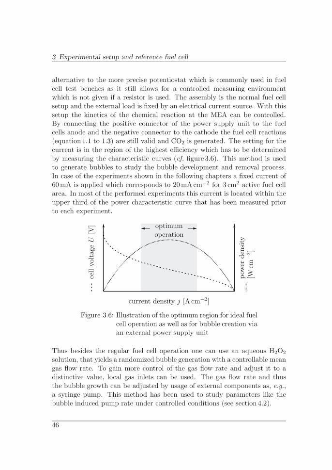
3 Experimental setup and reference fuel cell
alternative to the more precise potentiostat which is commonly used in fuelcell test benches as it still allows for a controlled measuring environmentwhich is not given if a resistor is used. The assembly is the normal fuel cellsetup and the external load is fixed by an electrical current source. With thissetup the kinetics of the chemical reaction at the MEA can be controlled.By connecting the positive connector of the power supply unit to the fuelcells anode and the negative connector to the cathode the fuel cell reactions(equation 1.1 to 1.3) are still valid and CO2 is generated. The setting for thecurrent is in the region of the highest efficiency which has to be determinedby measuring the characteristic curves (cf. figure 3.6). This method is usedto generate bubbles to study the bubble development and removal process.In case of the experiments shown in the following chapters a fixed current of60mA is applied which corresponds to 20mAcm−2 for 3 cm2 active fuel cellarea. In most of the performed experiments this current is located within theupper third of the power characteristic curve that has been measured priorto each experiment.
optimumoperation
current density j [A cm−2]
pow
erde
nsity
[Wcm
−2]
cell
voltag
eU
[V]
Figure 3.6: Illustration of the optimum region for ideal fuelcell operation as well as for bubble creation viaan external power supply unit
Thus besides the regular fuel cell operation one can use an aqueous H2O2
solution, that yields a randomized bubble generation with a controllable meangas flow rate. To gain more control of the gas flow rate and adjust it to adistinctive value, local gas inlets can be used. The gas flow rate and thusthe bubble growth can be adjusted by usage of external components as, e.g.,a syringe pump. This method has been used to study parameters like thebubble induced pump rate under controlled conditions (see section 4.2).
46
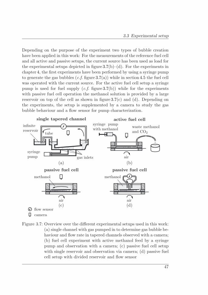
3.3 Experimental setup
Depending on the purpose of the experiment two types of bubble creationhave been applied in this work: For the measurements of the reference fuel celland all active and passive setups, the current source has been used as load forthe experimental setups depicted in figure 3.7(b)–(d). For the experiments inchapter 4, the first experiments have been performed by using a syringe pumpto generate the gas bubbles (c.f. figure 3.7(a)) while in section 4.5 the fuel cellwas operated with the current source. For the active fuel cell setup a syringepump is used for fuel supply (c.f. figure 3.7(b)) while for the experimentswith passive fuel cell operation the methanol solution is provided by a largereservoir on top of the cell as shown in figure 3.7(c) and (d). Depending onthe experiments, the setup is supplemented by a camera to study the gasbubble behaviour and a flow sensor for pump characterization.
(a) (b)
(c) (d)flow sensorcamera
single tapered channel active fuel cell
passive fuel cell passive fuel cell
tube
infinitereservoir
syringepump gas inlets
air air
air
syringe pumpwith methanol waste methanol
and CO2
methanol methanol
Figure 3.7: Overview over the different experimental setups used in this work:(a) single channel with gas pumped in to determine gas bubble be-haviour and flow rate in tapered channels observed with a camera;(b) fuel cell experiment with active methanol feed by a syringepump and observation with a camera; (c) passive fuel cell setupwith single reservoir and observation via camera; (d) passive fuelcell setup with divided reservoir and flow sensor
47

3 Experimental setup and reference fuel cell
Description of electrical fuel cell experiments
For the fuel cell performance measurements a setup consisting of a computercontrolled power supply with internal current measurement instrument (TTiPL330DP [77]) and an AD-card to acquire the voltage data as depicted infigure 3.8 were used. During the experiments, the data for the characteristiccurves and the long run measurement was logged every two seconds.
AV
anode
cathode
e−
current sourcefuel cell
Rfc Rwire
Rwire
Rwire
Figure 3.8: Diagram of the electrical experimental setupwith the fuel cell and the current source asload.
After fuelling the cell the first, the measurement of the characteristic curvefor an increasing current was performed. Together with the readout thenew current for the current source was set where the value is increased by∆ I = 2mA until the retrieved voltage is below zero. In the second part ofthe experiment the characteristic curve for decreasing current was measured.Identically to the first part, the current was decreased by ∆ I = 2mA everytwo seconds until I = 0mA is applied. For all experiments, the long runmeasurement was started after ten minutes. Starting the long run measure-ments after ten minutes ensured enough time to reach a stable open-circuitvoltage at zero applied current. This has been required since measuring timeof the characteristic curves were different for each fuel cell. The long runmeasurement was started by applying a current load of of I = 60mA. Thislast part of the measurement was automatically stopped when the voltagedropped below zero.
48
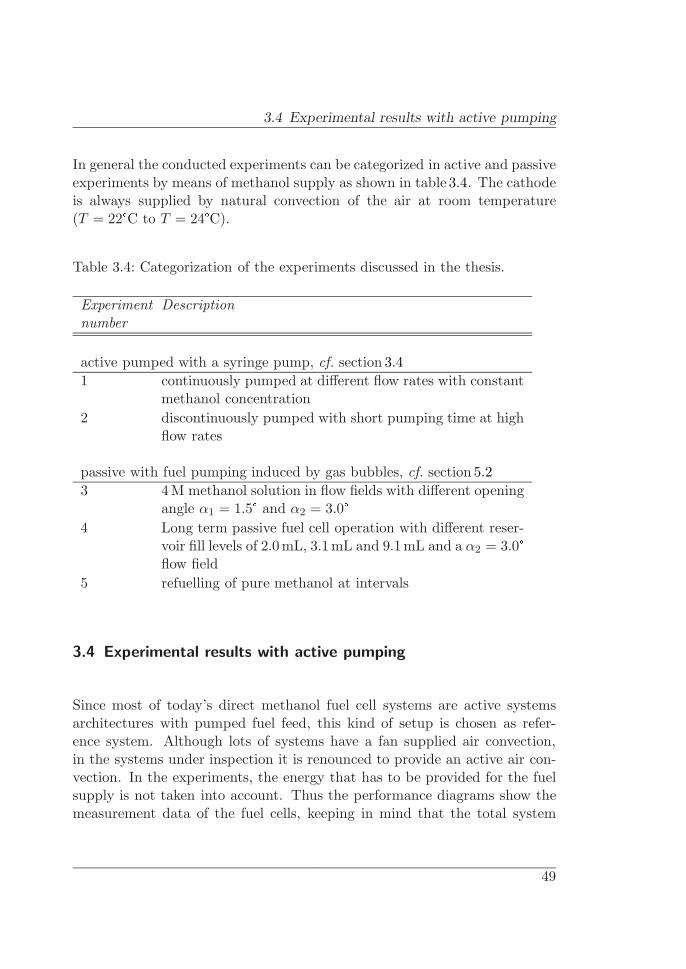
3.4 Experimental results with active pumping
In general the conducted experiments can be categorized in active and passiveexperiments by means of methanol supply as shown in table 3.4. The cathodeis always supplied by natural convection of the air at room temperature(T = 22�C to T = 24�C).
Table 3.4: Categorization of the experiments discussed in the thesis.
Experimentnumber
Description
active pumped with a syringe pump, cf. section 3.41 continuously pumped at different flow rates with constant
methanol concentration2 discontinuously pumped with short pumping time at high
flow rates
passive with fuel pumping induced by gas bubbles, cf. section 5.23 4M methanol solution in flow fields with different opening
angle α1 = 1.5� and α2 = 3.0�4 Long term passive fuel cell operation with different reser-
voir fill levels of 2.0mL, 3.1mL and 9.1mL and a α2 = 3.0�flow field
5 refuelling of pure methanol at intervals
3.4 Experimental results with active pumping
Since most of today’s direct methanol fuel cell systems are active systemsarchitectures with pumped fuel feed, this kind of setup is chosen as refer-ence system. Although lots of systems have a fan supplied air convection,in the systems under inspection it is renounced to provide an active air con-vection. In the experiments, the energy that has to be provided for the fuelsupply is not taken into account. Thus the performance diagrams show themeasurement data of the fuel cells, keeping in mind that the total system
49

3 Experimental setup and reference fuel cell
performance would be less when including internal energy consumption of anactive system architecture.
In the experiments a 4M methanol solution is provided through tubes bythe use of a syringe/perfusor pump of Braun Melsungen [78]. The schematicexperimental setup depicted in figure 3.9 shows the two tubes casted to thedrilled flow field samples. The methanol solution is pumped into the flowfield through the left tube and the unconsumed methanol together with thegas bubbles is flushed out through the tube on the right side. During theexperiment, the bubble development and removal can be inspected from thetop through the PMMA flow field.
air
methanolsolution
methanol solutionand CO2-bubbles
anode currentcollector
cathode cur-rent collector
membrane and gasdiffusion layers
flow field
upper mount-ing plate
lower mount-ing plate
Figure 3.9: Experimental setup for an active pumped sys-tem with tubes for fuel delivery and wasteremoval
Performance parameters in fuel cell experiments
To compare the different fuel cells in the experiment, the energy efficiency ηas ratio of the gained electrical energy Eel and the provided chemical energyWc,provided will be used.
η =Eel
Wc,provided(3.1)
50
3.4 Experimental results with active pumping
Eel can be determined by integrating P [W] over the runtime t [s]. In thiscalculation the energy consumption of peripherals is not included. To cal-culate the efficiency of the full system ηtotal the energy consumption of theperipherals Eel,peripherals has to be subtracted from Eel:
ηtotal =Eel − Eel,peripherals
Wc,provided(3.2)
As the syringe pump used for the active pumped system setups is not adedicated pump for portable fuel cell system Eel,peripheral is not included inthe calculation of η. Thus in the active system setups η is higher than ηtotal
would calculate.
In case of a passive system as depicted in figure 3.7(c) and (d) where a fixedamount of methanol is provided through the reservoir and all methanol isutilized by the fuel cell, the provided chemical energy Wc,provided can easilybe calculated. First, one has to calculate the energy contents Wc,MeOH [J L−1]of one litre methanol solution. Part of this equation is the number of electronsthat are provided during the reaction nel = 6e−, the Avogadro constant NA,the methanol concentration CMeOH [mol L−1] of the solution as well as theelementary charge e:
Wc,MeOH = CMeOH · NA · nel · e (3.3)
Now, the volume of pure methanol that is fed to the system needs to be cal-culated based on the molar volume of methanol vm,MeOH = 0.04051L mol−1
and the methanol concentration CMeOH [mol L−1] of the solution:
VMeOH = vm, MeOH · CMeOH (3.4)
In case of the passive system as depicted in figure 3.7(c) and (d) this equationis valid, as the methanol is fed to the reservoir and completely utilized duringthe fuel cell operation.
51

3 Experimental setup and reference fuel cell
For the active system as shown in figure 3.7(a), the situation is different sincethe methanol solution is pumped through the system and not all methanolis utilized while passing the membrane area. Thus, for the calculation of theprovided chemical energy one has to replace CMeOH in equation 3.3 by theinitial methanol concentration CMeOH,source subtracted by the concentrationat the outlet of the fuel cell CMeOH,outlet. In this case Wc,MeOH yields:
Wc,MeOH,active = (CMeOH,source − CMeOH,outlet) · NA · nel · e (3.5)
A similar replacement has to be done in equation 3.4 and in addition, theamount of methanol solution that is provided during the fuel cell operationhas to be calculated, using the flow rate φ and the runtime of the systemtrun. The volume of methanol in this case yields:
VMeOH,active = φ · trun · (CMeOH,source − CMeOH,outlet) · vm, MeOH (3.6)
Then, the chemical energy Wc,provided for a passive system and an activesystem can be calculated by multiplying Wc,provided with VMeOH,active:
Wc,provided,passive = C2MeOH · NA · nel · e · vm, MeOH (3.7)
Wc,provided,active = (CMeOH,source − CMeOH,outlet)2
·NA · nel · e · φ · trun · vm, MeOH (3.8)
With these formulas, the energy efficiency of a passive and an active systemsetup can be calculated. To determine the energy efficiency of active systemsthe methanol concentration of the outgoing flow has to be monitored andsubtracted. For the passive systems in chapter 5 the energy efficiency is cal-culated. Since the methanol concentration CMeoh,outlet in the outgoing flowwas not monitored, a comparison of the energy efficiencies between the activeand the passive systems in this work is only possible by the average powerdensity Pmean achieved during the experiments. Furthermore, the short andlong term reference values which are the performance of the active fuel cell
52
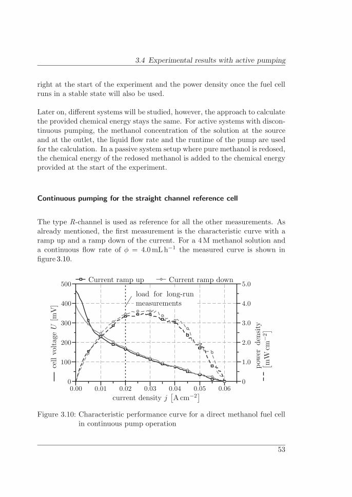
3.4 Experimental results with active pumping
right at the start of the experiment and the power density once the fuel cellruns in a stable state will also be used.
Later on, different systems will be studied, however, the approach to calculatethe provided chemical energy stays the same. For active systems with discon-tinuous pumping, the methanol concentration of the solution at the sourceand at the outlet, the liquid flow rate and the runtime of the pump are usedfor the calculation. In a passive system setup where pure methanol is redosed,the chemical energy of the redosed methanol is added to the chemical energyprovided at the start of the experiment.
Continuous pumping for the straight channel reference cell
The type R-channel is used as reference for all the other measurements. Asalready mentioned, the first measurement is the characteristic curve with aramp up and a ramp down of the current. For a 4M methanol solution anda continuous flow rate of φ = 4.0mL h−1 the measured curve is shown infigure 3.10.
current density j[Acm−2
]
cell
voltag
eU
[mV
]
pow
erde
nsity
[ mW
cm−2
]
load for long-runmeasurements
0.00 0.01 0.02 0.03 0.04 0.05 0.060
100
200
300
400
500
0
1.0
2.0
3.0
4.0
5.0Current ramp up Current ramp down
Figure 3.10: Characteristic performance curve for a direct methanol fuel cellin continuous pump operation
53

3 Experimental setup and reference fuel cell
The power performance is almost identical in both parts of the measurement.This is due to the continuous flow of the methanol solution where the bubblesare flushed out of the fuel cell. Only in the region of 0 ≤ j ≤ 0.01A cm−2
the measured voltage differs notably. The difference can be explained by thedifferent times where the data is collected during the experiment, which is atthe beginning and the end of the data acquisition for the performance curve.At the start of the experiment, the system is primed with fresh methanol so-lution and no gas bubbles are inside the flow field. Furthermore, there is nogeneration of gas bubbles since no methanol is consumed. During the currentramp up and the following ramp down, gas bubbles are generated and mostof them are flushed out immediately. However, at the end of the performancecurve measurement, there are still some gas bubble in the flow field. Hence,the active area is still partly covered with gas and thus the resulting perfor-mance is worse. At the peak performance, both curves are almost identicaland minor differences can be traced back to the bubble generation on theMEA which is not an absolutely regular event.
In case of higher liquid flow rates these differences and the performance donot change significantly. For lower flow rates, however, the gas bubbles arenot rinsed out that fast and thus the performance decreases continuously overtime.
For the long term measurement starting after 10min, the power density de-creases from a start value of Pstart = 3.7mW cm−2 and stabalizes at a value ofPstable = 1.6mW cm−2 as shown in figure 3.11. In the continuously pumpedexperiments, the fuel cell shows a decreasing performance curve during thefirst hours of the measurement. Since the methanol is continuously pumpedthrough the fuel cell at a flow rate that ensures sufficient methanol at themembrane, the reason for the performance drop can be ascribed to the cath-ode side of the fuel cell. As passive air convection is used at the cathode,the produced water or water vapour at this side is not sufficiently removed.During the reaction on the cathode side water droplets form in the cathodeflow field. These water droplets block parts of the membrane area and theblocked area increases over time and yields a decreasing power performance ofthe cell. Once the droplets have grown to a certain size, they tear off and thefree active area increases again resulting in a power increase. Those tear offevents are responsible for the sudden performance increases after t = 0.5 h,
54

3.4 Experimental results with active pumping
t = 1.75 h and t = 3.5 h. After t = 3.5 h runtime, the performance curvestabilized at the value of about Pstable = 1.6mW cm−2 until the experimenthas been stopped after four hours.
type R
pow
erde
nsity
[ mW
cm−2
]
t [h]
0
1
2
3
4
5
1 2 3 4 5 6 7 8 9 10
Figure 3.11: Long time performance curve of a pumped type R fuel cell start-ing at Pstart = 3.7mW cm−2 and reaching a stable power outputof Pstable = 1.6mW cm−2 after t = 3.5 h runtime.
Continuous pumping in passive flow field structures
The same type of measurement as discussed in the previous section has beenperformed on the channel types A and B. All three fuel cells are in the samemounting and the experiments have been conducted successively by connect-ing the syringe pump to the next fuel cell. Since the flow rate, methanolconcentration and the measurement setup are identical, it can be expectedthat the resulting power density for all three channel types are identical.Thus this experiment can be used as measure for the repeatability of theexperiments performed in this work.
The curves for type A and B start at values of PA,start = 4.1mW cm−2 andPB,start = 3.7mW cm−2 as shown in figure 3.12. In general the curve shapes
55

3 Experimental setup and reference fuel cell
for these two channels show the same distribution as the type R-channel. Thestart value under load of I = 60mA is the same as the previously measuredvalue from the characteristic curve. The average short term power densityPref,str of these three curves is 3.8mWcm−2 with a standard deviation of0.23mWcm−2. All curves first decrease, showing some sudden performanceincreases when a water droplet tears of at the cathode side. This effect hasbeen observed in most of the experiments. After three hours of measurementthey stabilize at values of PA = 1.65mW cm−2 and PB = 1.32mW cm−2.Some performance peaks above these limit values can be identified. Thus forthe continuously pumped mode all channels show basically the same perfor-mance behaviour with a decreasing power during the first two to three hoursand a stable limit value. The variation between the different curves is maxi-mum 1mW cm−2 which will be used as measure whether differences betweenthe channels in the experiments can be considered as significant. The meanlong run power density Pref,lrr for the three pumped fuel cell experimentswith the channels R, A and B is 1.5mWcm−2 with a standard deviation of0.2. This value of Pref,lrr will be used as reference and all experiments willbe compared to this value. Parameters that can affect the variation betweenthe different channels are the temperature in the fuel cell, the location andthe amount of different water droplets that form on the cathode as well asminor geometrical differences of the fuel cells due to the assembly process.
Conclusion
As all three fuel cells initially start at Pstart = 3.7–4.1mW cm−2 and thenstabilize over time in the range of Plong term = 1.32–1.65mWcm−2 it can beconcluded that the three channel types are acting identically with a varia-tion of maximum ±0.5mW cm−2 around the long run reference of Pref,lrr =1.5mWcm−2, as anticipated. The measurements show that the results arerepeatable with a certain range of variation due to water formation, temper-ature differences and geometrical differences due to the assembly process.
56

3.4 Experimental results with active pumping
type R type A type B
pow
erde
nsity
[ mW
cm−2
]
t [h]
short term refer-ence Pref,str
long run refer-ence Pref,lrr
0
1
2
3
4
5
1 2 3 4 5 6 7 8 9 10
Figure 3.12: Long term performance for continuous pumped fuel cells withflow field channels of the type R, A and B and the limit values ofPR = 1.6mW cm−2, PA = 1.65mW cm−2 and PB =1.32mW cm−2.
Discontinuous pumping in passive flow field structures
One approach to increase the performance of an active fuel cell system can beby intelligent supply methods. Since the fuel cells are commonly supplied byan integrated continuously running pump, this is one possible part where thesystem energy demand can be reduced. One approach is to run the pump ina discontinuous mode where the pump is deactivated most of the time, whichhas already been shown as an early experiment in [17, 46].
This has been done for a flow rate of 40.0mL h−1 at intervals of 0.5min activepumping and 9.5min passive operation with a 4M methanol solution in a flowfield with an opening angle of α2 = 3� for the channel types A and B. Bychoosing this flow-rate and pumping interval, the amount of methanol thatis pumped through the fuel cell is equivalent to the continuously pumpedsystem, studied before. The measurement results in figure 3.13 show theperformance curve over 17 pump intervals for the channels of type R and
57
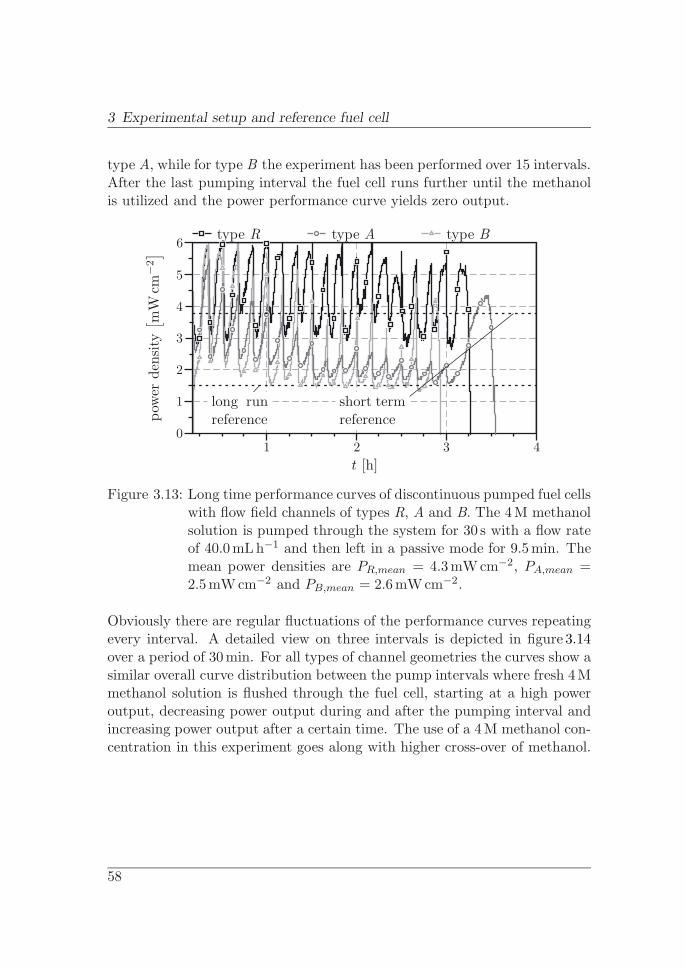
3 Experimental setup and reference fuel cell
type A, while for type B the experiment has been performed over 15 intervals.After the last pumping interval the fuel cell runs further until the methanolis utilized and the power performance curve yields zero output.
type R type A type B
pow
erde
nsity
[ mW
cm−2
]
t [h]
long runreference
short termreference
0
1
2
3
4
5
6
1 2 3 4
Figure 3.13: Long time performance curves of discontinuous pumped fuel cellswith flow field channels of types R, A and B. The 4M methanolsolution is pumped through the system for 30 s with a flow rateof 40.0mL h−1 and then left in a passive mode for 9.5min. Themean power densities are PR,mean = 4.3mWcm−2, PA,mean =2.5mWcm−2 and PB,mean = 2.6mWcm−2.
Obviously there are regular fluctuations of the performance curves repeatingevery interval. A detailed view on three intervals is depicted in figure 3.14over a period of 30min. For all types of channel geometries the curves show asimilar overall curve distribution between the pump intervals where fresh 4Mmethanol solution is flushed through the fuel cell, starting at a high poweroutput, decreasing power output during and after the pumping interval andincreasing power output after a certain time. The use of a 4M methanol con-centration in this experiment goes along with higher cross-over of methanol.
58

3.4 Experimental results with active pumping
type R type A type B
pow
erde
nsity
[ mW
cm−2
]
t [min]
long runreference
short termreference
pumpinginterval
0
1
2
3
4
5
6
60 70 80 90
Figure 3.14: 30min excerpt of the discontinuous pumped experiment to clar-ify the influence of the pumping onto the system.
This effect can be observed when the pump is activated as shown in figure 3.15as slope 1. The high methanol concentration yields higher cross-over andtherefore the performance of the fuel cell is reduced significantly within 2minof the experiment after the activation of the pump. In addition all the gasbubbles are flushed out of the fuel cell during the pumping interval leading toa completely liquid filled flow field with high methanol concentration. A lowerflow rate would slow down the effects that cause the performance decreaseand the slope will be less steep. In the actual case the slope is identical forall three channels, according to the identical flow rate.
After deactivation of the pump the liquid convection is only induced by thedeveloping gas bubbles that move towards the liquid outlet. This yields anincreased coverage of the active area by gas bubbles. Furthermore duringthe fuel cell operation the local concentration of the methanol solution in theflow-field decreases, going along with a decrease of methanol cross-over. Inconsequence the performance increases until either the methanol is consumedor the next pumping interval supplies new methanol. This is indicated byslope 2 of figure 3.15 where the time between t1 and t2 is determined by thevolume of the methanol solution in the channel and the slope is proportionalto the coverage of the active area with methanol/CO2.
59

3 Experimental setup and reference fuel cell
power density curvepo
wer
dens
ity
t
slope 1 ∝ pump rate
slope 2 ∝MeOH/CO2
coverage
0t0 t1 t2 t3
Figure 3.15: Schematic diagram of the power density curve and the typicalslopes after the pumping (t0–t1), when the MEA is covered withmethanol/CO2 (t1–t2) and the run-out of the fuel cell (t2–t3).
When proceeding with a new pump cycle, a sharp performance peak can beobserved prior to the significant decrease of the performance related to theincreased cross-over. The performance peak is caused by the combination ofa sudden increase of methanol concentration while the methanol cross-overis still low. In case no new fuel is delivered, the performance decreases withdecreasing methanol concentration until P = 0.
Although the overall curve distribution is comparable for the three chan-nel types, the curves differ in detail. In case of the flow field types A andB the pumping interval already delivers new fuel while the performance isstill increasing as shown in figure 3.14. The performance of the type R flowfield reaches its maximum performance between the pump intervals or evendecreases already. This is due to the fact, that characteristic performance(U -I-curve) is different for the different cell types such that the operatingpoints are different in the experiment. In consequence this means that theeffective power generation is smaller and the fuel utilization is lower for cellsA and B and thus they are refuelled too early.
Furthermore the three channel types differ in the amount of methanol con-tained in the flow field which affects the performance curves. The type
60
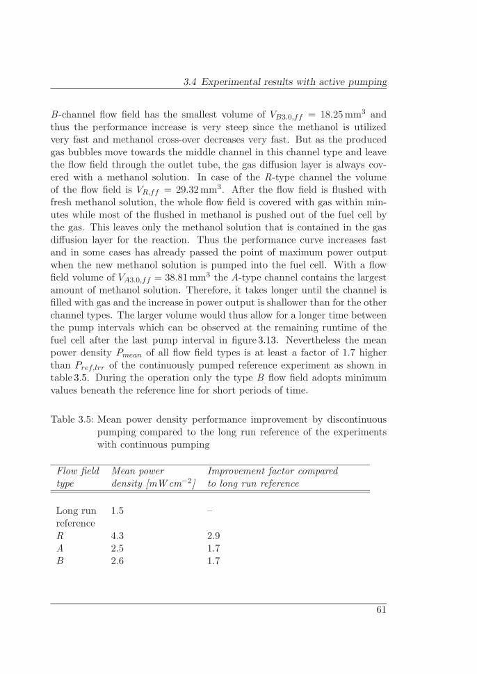
3.4 Experimental results with active pumping
B-channel flow field has the smallest volume of VB3.0,ff = 18.25mm3 andthus the performance increase is very steep since the methanol is utilizedvery fast and methanol cross-over decreases very fast. But as the producedgas bubbles move towards the middle channel in this channel type and leavethe flow field through the outlet tube, the gas diffusion layer is always cov-ered with a methanol solution. In case of the R-type channel the volumeof the flow field is VR,ff = 29.32mm3. After the flow field is flushed withfresh methanol solution, the whole flow field is covered with gas within min-utes while most of the flushed in methanol is pushed out of the fuel cell bythe gas. This leaves only the methanol solution that is contained in the gasdiffusion layer for the reaction. Thus the performance curve increases fastand in some cases has already passed the point of maximum power outputwhen the new methanol solution is pumped into the fuel cell. With a flowfield volume of VA3.0,ff = 38.81mm3 the A-type channel contains the largestamount of methanol solution. Therefore, it takes longer until the channel isfilled with gas and the increase in power output is shallower than for the otherchannel types. The larger volume would thus allow for a longer time betweenthe pump intervals which can be observed at the remaining runtime of thefuel cell after the last pump interval in figure 3.13. Nevertheless the meanpower density Pmean of all flow field types is at least a factor of 1.7 higherthan Pref,lrr of the continuously pumped reference experiment as shown intable 3.5. During the operation only the type B flow field adopts minimumvalues beneath the reference line for short periods of time.
Table 3.5: Mean power density performance improvement by discontinuouspumping compared to the long run reference of the experimentswith continuous pumping
Flow field Mean power Improvement factor comparedtype density [mWcm−2] to long run reference
Long run 1.5 –referenceR 4.3 2.9A 2.5 1.7B 2.6 1.7
61

3 Experimental setup and reference fuel cell
Conclusion
As shown in the experiment with fixed time intervals, there is an improve-ment of the power performance independent of the flow field geometry whencompared to the reference experiment of more than 1.7× for the mean powerperformance. This denotes that a performance improvement can be achievedfor most persisting active DMFC systems by using a discontinuous pumpingmethod while delivering the equivalent amount of methanol. The improvedperformance is resulting from the decreasing methanol cross-over during thepassive interval. In this interval, the methanol concentration continuouslydecreases until new methanol solution is pumped into the fuel cell.
By adapting the duration of active and passive intervals, the pump can beoperated in the point of its maximum energy and pump efficiency. Furtherimprovement can be expected by changing from fix time intervals betweenthe pumping to fuel cell power performance driven intervals, e.g., by startingthe pump at the fuel cells peak power density. Nevertheless, these measure-ments already led to a power density performance improvement of more than1.7× compared to the reference experiment. After having shown that a per-formance improvement by discontinuous pumping is feasible, further studiesof the way of operating the fuel cell can be an objective for future work.Especially to determine the correlation between the gradient of slope 2 asfunction of the coverage of the active area by methanol/CO2 can help tooptimize the fuel cell operation. The balance between the passive operationand the pumping intervals and high output power performance due to a fastperformance increase after the pump interval has to be found in order to gainmaximum system power performance.
62

4 Passive pumping in simulation and experiment
In this chapter it is shown by simulation and experiments that methanol so-lution can be passively pumped at a flow rate sufficient for passive long termfuel cell operation. The first part of this chapter deals with the modelling offuel cells and how computational fluid dynamics simulations (CFD) can beused to study bubble dynamics in tapered structures. Then the minimumrequired methanol flow rate required for passive long term fuel cell operationis determined based on the boundary conditions of the methanol concentra-tion, the fuel cell’s load and active area. With the known required theoreticalminimum flow rate simulations and experiments with single type A and Bchannels and a reservoir that allows fuel recirculation outside the flow fieldare studied. The gas flow rate to grow the CO2 bubbles was generated byusing mass source terms in the simulation model and a syringe pump in theexperiments. Succeeding the studies with single channels the liquid flow rategenerated during fuel cell operation in R, A and B-type flow fields is measuredwith a flow sensor and compared to the required minimum flow rate.
4.1 CFD-modeling
Modelling a complete direct methanol fuel cell system is rather complex sincea huge variety of parameters affect the system, e.g. temperature, chemical re-actions, surface effects and liquid-gas-flow. Thus the system can be modelledby dividing it into different problems, while keeping the other parameters inmind to set the correct boundary conditions. For modelling the gas bubble de-velopment, movement and the bubble induced convection, the computationalfluid dynamics software package CFD-ACE+ [79] was used. Like many otherCFD-software packages the code of CFD-ACE+ is based on the finite-volumemethod (FVM)[80] to solve the Navier-Stokes equations. The velocity pres-sure coupling is generally accomplished by the SimpleC algorithm [80] which
63

4 Passive pumping in simulation and experiment
was original proposed by Vandoormaal and Raithby [81] or slight variations ofit like the so called SOLA algorithm [82–85]. Furnished with these algorithmstypical problems of incompressible laminar viscous flow can be addressed.
For modelling free surface flows the Volume of Fluid (VOF) method as pro-posed first by Hirt and Nichols [86] and refined later on by various authors[87–91] is applied. It is based on tracking a scalar field variable F whichstands for the distribution of the second fluid in the computational grid. Fspecifies the fraction of the volume of each computational cell in the gridoccupied by the second fluid. All cells containing only fluid two will takethe value F = 1, and cells completely filled with fluid one are represented byF = 0. Cells containing an interface between fluid one (e.g. air) and fluid two(e.g. water) take on a value of F between 0 and 1. For a given flow-field withthe velocity vector �v and an initial distribution of F on a grid, the volumefraction distribution F (and hence the distribution of fluid two) is determinedby the passive transport equation:
∂F
∂t+ ∇�v F = 0 (4.1)
This equation must be solved together with the fundamental equations of con-servation of mass and momentum, to achieve computational coupling betweenthe velocity field solution and the liquid distribution. From the F distribu-tion the interface between the two fluid phases has to be reconstructed atevery time step. CFD-ACE+ uses the piecewise linear interface construction(PLIC) scheme [88] for this purpose.
The position, shape and especially the curvature of the free surface are re-quired to determine the capillary forces given by the Young-Laplace equation[80, 92–95]. Typically these surface forces are included into the algorithmas body forces in those cells containing the interface i.e. having F -valuesbetween 1 and 0 [86, 88]. Contact angles at the fluid/solid interface areaccounted for in a similar way [96].
For solving the numerical equation systems two types of solvers are availablein CFD-ACE+: The adaptive multi grid solver (AMG) and the conjugategradient solver (CGS) [97, 98].
64

4.1 CFD-modeling
In CFD-ACE+ the VOF-method offers some additional features like an algo-rithm to remove the so called flotsam and jetsam. This is an artefact causedby numerical errors, and is characterized by the generation of tiny isolateddroplets of liquids or gas in the regions of the other medium, especially inregions of high swirl. A further feature is given by the capillary wave dampingwhich allows for locally increasing the viscosity in the vicinity of the interfaceenabling larger time steps since tangential velocities are reduced.
Modelling approach
Modelling two phase flow with liquid and gas on the anode side of a DMFCwith a CFD-code, one has to face several problems: First, the channeldimensions and the methanol reaction rate versus the time needed for a bub-ble to exit the channel yields a spatial and temporal multi-scale problem:On the one hand a single fuel cell channel has a length of 20mm versus thesmallest length of the channel 0.3mm (see tableB.1 of the annex) that hasto be covered with minimum 10 grid cells to sufficiently describe the bubbledevelopment and movement in the channel. This yields a large simulationmodel due to the geometry. On the other hand, the bubbles develop withinless than a second leading to simulation time steps in the order of microsec-onds. But to drive a bubble out of one fuel cell channel takes more thanseveral seconds yielding a large number of time steps for the simulation thattakes up to several weeks of simulation time. Second, the physics involvedis rather complex in terms of flow through a porous media (GDL), dynamiccontact angle, contact angle hysteresis or pinning, influence of the bubblecoalescence behaviour and thin film dynamics. All these aspects are no stan-dard problems for CFD and one has to consider carefully whether they havea significant influence on the fluid dynamics or when they can be neglected.
Figure 4.1 shows a sketch of the anode side of a methanol fuel cell with all theelements that influence the system, the membrane, the gas diffusion layer, theflow-field channel with the fuel and waste, the gas outlet and the recirculationloop coupled to the reservoir with a constant methanol concentration. Theseelements have to be modelled in different ways for an effective simulationstudy of a direct methanol fuel cell. The membrane electrode assembly andits electro kinetics is often modelled as 1-D or 2-D model [99–103]. Since
65

4 Passive pumping in simulation and experiment
this is a research field of its own and far beyond the scope of this thesis,no detailed modelling of the membrane is performed and the volume of gasproduced during the methanol reaction is provided as a boundary condition.The gas diffusion layer can be modelled in CFD by a porous media volumetricboundary condition where the gas can pass through. However, as CFD-ACE+does not allow to combine a porous media model with VOF, one has to omiteffects like methanol flow through the gas diffusion layer and pinning effectsof the gas bubbles. The flow-field channel itself can be modelled with CFDto cover fuel transportation, bubble development and movement as well asseparation of the gas from the liquid by applying the according boundaryconditions. As in the used models the methanol consumption out of thesolution is not implemented, only the inlet and outlet boundary conditionscan be applied. In case the methanol consumption at the membrane wouldbe modelled as well, a reservoir with constant methanol concentration couldbe coupled to the system by using a network model approach.
1
2
345a 5b
6
Figure 4.1: Modelling of a direct methanol fuel cell where the channel struc-ture (2) is modelled by CFD. The boundary conditions for thegas diffusion layer (3), the inlet (5a), the outlet (5b), and thegas outlet (1) are modelled as a network. The MEA (4) with itselectrokinetics is given as boundary condition for the GDL (3).The infinite reservoir with constant methanol concentration (6)determines the boundary condition for the liquid inlet (5a) andoutlet (5b).
66

4.1 CFD-modeling
Verification of bubble movement in tapered structures
One example for the impact of the details of the CFD-model on the agreementbetween simulations and experiments can be given by the movement of gasbubbles in tapered channels as shown as sketch of the experimental setup infigure 4.2(a) [104]. A camera is used to monitor the dynamics of gas bubblesmoving between two planes in a tapered configuration with an opening angleα. The gas is induced through a small pipe into a liquid filled tapered slitformed by two microscope slides arranged in a defined angle α. The liquiditself stays in the slit due to capillary forces (θ � 90 �). Since the slit is toosmall to allow the gas bubble to adopt a spherical shape, which correspondsto the minimum energy, it is deformed. This yields a lenticular shape withdifferent radii at the distant ends of the gas bubble. The different radii yielddifferent capillary forces and thus a pressure gradient along the bubble. Oncethe bubble has grown to a critical size it detaches from the pipe as depicted infigure 4.2(b) and moves along the widening channel, in the figure from left tothe right. The velocity of the bubble decreases the further it moves towardsits equilibrium position. In this position the liquid-gas interface has a uniformcurvature, a spherical shape, and thus reached its equilibrium state.
With the aid of the camera it is possible to determine the distance betweenthe bubble and the intersection line of the two planes, formed by the glassslides. Figure 4.2(c) shows the comparison of the experimental data withCFD-simulations [104]. By using the standard CFD-model with constantcontact angle, i.e. the simplest possible simulation setup, the bubble velocityis overestimated by the CFD-solver with approximately 20%. The large quan-titative deviation can be traced back to three main causes: The disregard ofdynamic contact angles, surface roughness and liquid thin films.
The dynamic contact angle is disregarded and the contact angle θ of theliquid-gas-interface with the wall is given as static parameter. This yields thatadvancing and receding contact angles are not modelled accurately within theused models. Thus the dynamics at the three-phase boundary is not reflectedcompletely in the CFD-code which results in a reduced pressure gradient overthe gas bubbles length.
The surface roughness is disregarded as the wall of the simulation model isassumed to be ideally plain. A real wall always shows surface roughness that
67

4 Passive pumping in simulation and experiment
(a)
cameraslide
pipe
pipe
liquid
α
l
(b)
0.0 s0.02 s0.06 s0.09 s0.12 s0.16 s0.29 s0.78 s
1 mm
(c)t [s]
x[m
m]
0.00 0.05 0.10 0.15 0.20 0.25 0.30 0.35 0.400
2
4
6
8
10
12
14
exp. data mean exp. data
CFD reference
Figure 4.2: Experimental setup to determine the bubble movement betweentwo glass slides arranged to form a tapered slit (a) and a framesequence of the experiment as top view (b). Accumulating theexperimental data of the bubble centre positions x over the timeyields the a curve that can be benchmarked against by CFD-simulations (c) [104]
plays a significant role in sub-millimetre dimensions [105, 106]. The dynamicsof the interfacial surface is reduced as the surface roughness influences pinningeffects.
Liquid thin films that can be observed in experiments between the moving gasbubble and the channel walls are disregarded as well. This thin liquid filmsexhibit large shear forces due to the bubble movement and thus the bubbledynamics is reduced. This film is not accounted for by the CFD simulations.
Each of the phenomena mentioned above are separate fields of research and of-ten addressed by different simulation approaches, e.g., by moleculardynamics simulations [107].
68

4.2 Required methanol flow for continuous passive fuel cell operation
Conclusion
The study of bubble movement in tapered channels by using CFD-methodsreveals that modelling of this class of problems with low driving forces inducedby differences in the capillary pressure is still challenging for CFD-softwaretools which was a conclusion made in [108]. Thus it is a prerequisite thatfor problems like this careful modelling and validation of the simulations hasto be carried out before quantitative results can be expected. Nevertheless,although the results cannot be expected to yield quantitative values, theycan be assumed to be qualitatively correct. To further increase the accuracydoes not necessarily yield further basic findings. By knowledge that the wallroughness can not be modelled in detail, the overestimated velocities can beaccepted if the main task is to proof the working principle of e.g. a bubblepump. Proceeding to the modelling of bubbles in channels as done in thenext section, one has to keep in mind that the overestimated velocities mightinfluence the quantitative results there, whereas the qualitative results interms of bubble dynamics can be expected to be correct.
4.2 Required methanol flow for continuous passive fuel celloperation
Whether it is possible to realize a pumping mechanism, driven by the CO2
produced during the fuel cells operation, has been a central question duringthis work. To achieve a directed convective liquid flow it is essential to controlthe movement of the gas bubbles. Another way of directing the flow and, inaddition, implementing the driving mechanism is to use tapered channels,in the present case the channel types A and B. Prior to implementing thisdriving mechanism into a fuel cell, it has been studied in simulations andexperiments.
Once it has been proven, that pumping in general is possible, the next step isto proof that the generated flow rate is high enough to sustain long term fuelcell operation. The minimum flow rate of the methanol solution φmin, MeOH, sol
to enable continuous fuel supply can be determined by calculating the
69
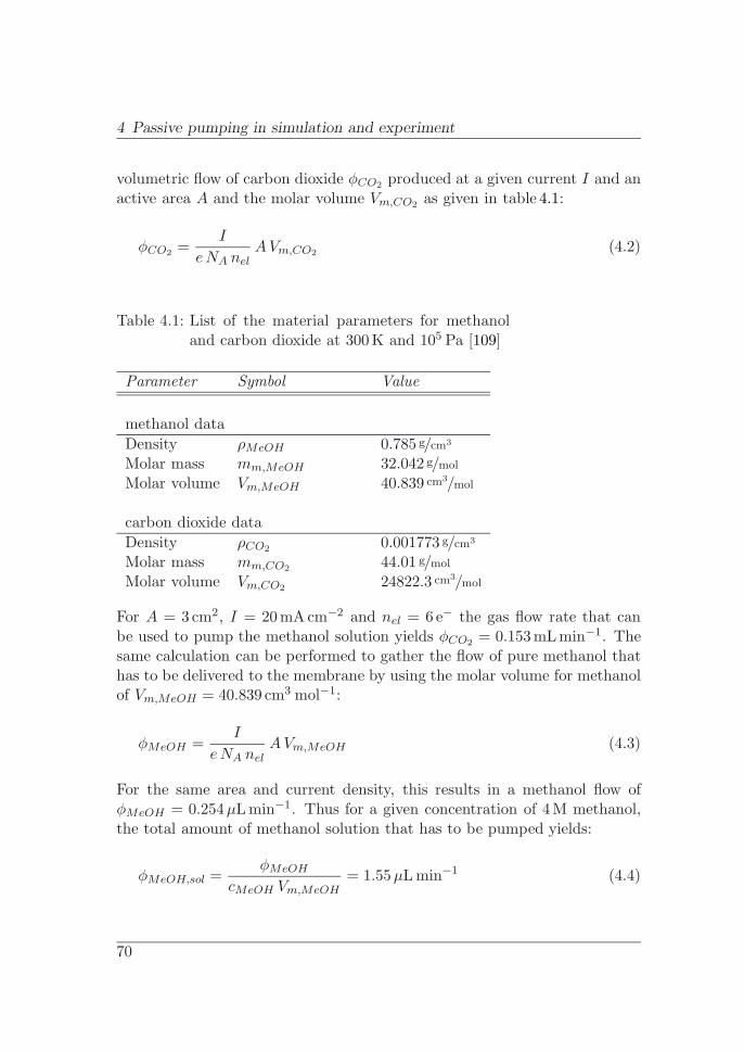
4 Passive pumping in simulation and experiment
volumetric flow of carbon dioxide φCO2 produced at a given current I and anactive area A and the molar volume Vm,CO2 as given in table 4.1:
φCO2 =I
eNA nelAVm,CO2 (4.2)
Table 4.1: List of the material parameters for methanoland carbon dioxide at 300K and 105 Pa [109]
Parameter Symbol Value
methanol dataDensity ρMeOH 0.785 g/cm3
Molar mass mm,MeOH 32.042 g/mol
Molar volume Vm,MeOH 40.839 cm3/mol
carbon dioxide dataDensity ρCO2 0.001773 g/cm3
Molar mass mm,CO2 44.01 g/mol
Molar volume Vm,CO2 24822.3 cm3/mol
For A = 3cm2, I = 20mAcm−2 and nel = 6e− the gas flow rate that canbe used to pump the methanol solution yields φCO2 = 0.153mL min−1. Thesame calculation can be performed to gather the flow of pure methanol thathas to be delivered to the membrane by using the molar volume for methanolof Vm,MeOH = 40.839 cm3 mol−1:
φMeOH =I
eNA nelAVm,MeOH (4.3)
For the same area and current density, this results in a methanol flow ofφMeOH = 0.254µL min−1. Thus for a given concentration of 4M methanol,the total amount of methanol solution that has to be pumped yields:
φMeOH,sol =φMeOH
cMeOH Vm,MeOH= 1.55µL min−1 (4.4)
70

4.3 Flow rate studies in simulations
This yields a required pump efficiency for a 4M methanol solution of ηpump =φMeOH,sol
φCO2= 0.01. In terms of continuous fuel cell operation, the flow of 4M
methanol solution has to be minimum 1% of the generated gas volume.
Conclusion
The minimum required flow rate of the methanol solution φMeOH,sol thatis required to achieve a sustaining long term operation of the passive fuelcell has been derived. In case of a 4M methanol solution this flow rate isφMeOH,sol = 1.55µL min−1 and corresponds to a pump efficiency ηpump =φMeOH ,sol
φCO2= 0.01 that has to be achieved in fuel cell operation.
4.3 Flow rate studies in simulations
In this section the objective of the CFD simulation is to proof that withthe chosen channel designs A and B a liquid flow rate can be generated bymoving bubbles. Standard VOF methods have been applied to track the freeinterfaces with a static contact angle of θ = 35� taken from measurements of a4M methanol solution on PMMA. With respect to symmetry, only half of onesingle channel was simulated. The flow-field channel has been modelled witha partially liquid filled reservoir on top to allow recirculation of the liquidas shown in figure 4.3. To model the gas development the following electro-chemical model has been used: A constant current density of 120mAcm−2
was assumed for the simulation. Based on this current density and accordingto equation 1.1, where for every six charge pairs one CO2 molecule is gener-ated, the CO2 flow rate results in 307µL min−1 cm−2. It is assumed that theliquid is saturated with CO2, therefore, all generated CO2 will form bubbles.As discussed in the previous section the required pump efficiency yields aminimum required liquid flow rate of φliq ≥ 0.01φCO2 and yields for this sim-ulation a minimum liquid flow rate of 3.07µL min−1 for a channel that covers1 cm2 of the membrane. As material data for the simulation the propertiesof CO2 have been used as given in table 4.1. In case of the methanol solutionthe properties of water have been used as given in the material database of
71

4 Passive pumping in simulation and experiment
CFD-ACE+ [79]. The methanol fraction in the solution has been omittedsince it is only 16 percent by volume and it is assumed that liquid propertiesremain similar to water.
liquid
gas bubbles
partially liquidfilled reservoir
supply channels
flow-field channel
Figure 4.3: Simulation model of a single flow-field channelconnected to the partially liquid filled reservoirvia supply channels.
In comparison to the gas bubble generation method used in the simulationshown in figure 2.5 the gas bubbles in this model are generated by using masssource terms. Since the objective of the simulation is the study of the be-haviour of the grown gas bubbles and the liquid flow rate they generate overa few seconds simulation time, a method had to be found allowing genera-tion of sufficiently big gas bubbles within a short time while reducing thecomputational time required. Based on simulation studies by Paust [110] theapproach to use mass source terms for the gas bubble nucleation yields areduction of computational time by a factor of ten and the gas bubbles couldbe generated within milliseconds while not causing errors in the final result.
To comply with the real situation, the gas bubbles must be generated at thechannel bottom with a dynamic fulfilling equation 4.2. A gas bubble has to fillat least 83 grid cells as required by the Continuum Surface Force (CSF) model[96] in combination with PLIC; otherwise the calculated surface curvatureswithin the CSF model are inaccurate and cause instabilities. Smaller bubbles,≤ 83 grid cells, are of minor importance as their liquid gas interfaces do notcontribute to the capillary induced pump mechanism.
Within this modelling approach of the speed to grow the initial bubble is themost critical part, since growing the gas bubble at too high speed yields high
72

4.3 Flow rate studies in simulations
velocities in the surrounding liquid. Growing at too low speed results in anunstable simulation as the growing bubble is not calculated correctly in theCFS model. The best time scale for the initial bubble growth out of 2×4×4source cells to the minimum size of 83 cells has been identified iterativelyand is in the order of 40 time steps. By using a higher dynamic, where83 cells are filled with gas in less than 10 time steps, the strong velocitiesof rapidly growing bubbles cause divergence. Using a low growth rate of≥ 80 time steps to fill 83 cells in the other hand yield strong curvatures ofbubbles filling the 2×4×4 cells. This causes divergence as well, now becauseof the high capillary pressures. The developed method is used exclusivelyto generate gas bubbles in a channel avoiding divergence in the momentumequation and does not concur with the physics of bubble nucleation. Thedisplacement of liquid by these artificially growing bubbles certainly causessome errors within the simulation. However, this error is comparably smallwhen analysing the integral value of liquid, pumped by the movement of gasbubbles. Once a control volume contains a gas bubble, all generated CO2
calculated by equation 4.2 is added directly to the bubble through sourceterms in the continuity equation [111], now evenly distributed across theliquid gas interfaces occurring in each control volume.
In the model with a typical grid cell size of 30 × 30 × 30µm3, four discretevolumes of 4×4×4 grid cells defined as mass sources have been defined at themembrane side of the channel. Each of these volumes is used to generate a gasbubble. The CO2 generation is defined high enough to grow the bubble. Oncethe gas bubble has grown enough and touches the upper channel wall it getsdeformed and starts to move as described earlier. Although this model usesdiscrete bubble sources and thus does not fully represent a fuel cell modelit allows to quickly asses the gas bubble behaviour and their effect on theliquid flow rate in different channel types. Furthermore it allows the directcomparison of the results to experimental studies on the pumping potentialof different channels by using discrete bubble sources as well (cf. section 4.4).
One result of the simulations shown in figure 4.4 is the passive way of removingthe gas bubbles out of the channel. Furthermore the liquid flow inducedduring the bubble movement is sufficient to feed the fuel cell with new watermethanol solution. The necessary liquid flow of a 4M methanol solutioncorresponds with 1% of the volumetric gas flow of CO2. In the simulation
73
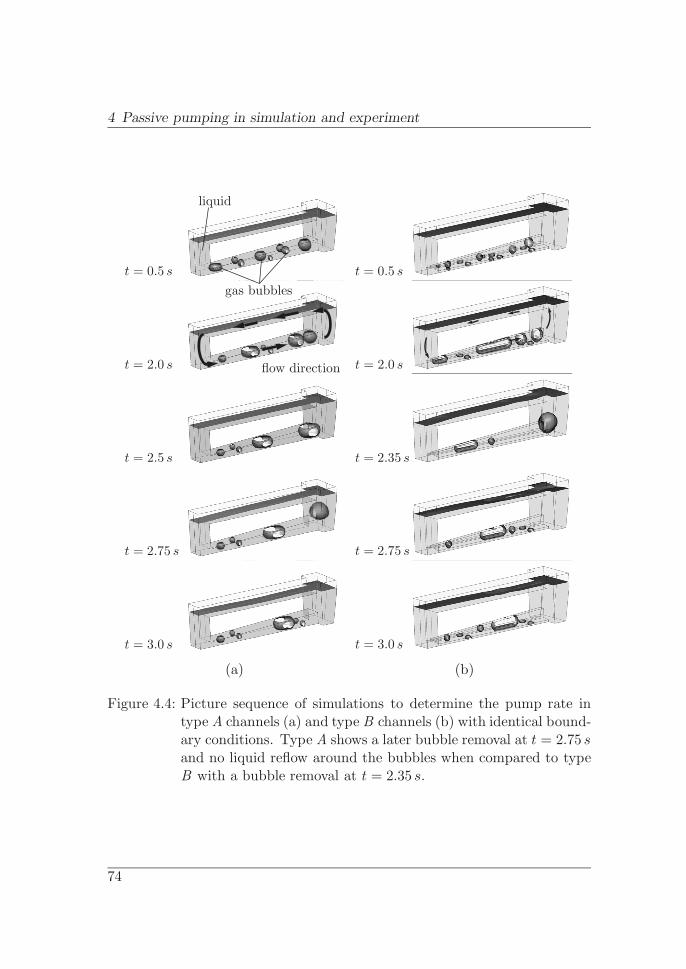
4 Passive pumping in simulation and experiment
(a) (b)
liquid
gas bubbles
flow direction
t = 0.5 s
t = 2.0 s
t = 2.5 s
t = 2.75 s
t = 3.0 s
t = 0.5 s
t = 2.0 s
t = 2.35 s
t = 2.75 s
t = 3.0 s
Figure 4.4: Picture sequence of simulations to determine the pump rate intype A channels (a) and type B channels (b) with identical bound-ary conditions. Type A shows a later bubble removal at t = 2.75 sand no liquid reflow around the bubbles when compared to typeB with a bubble removal at t = 2.35 s.
74
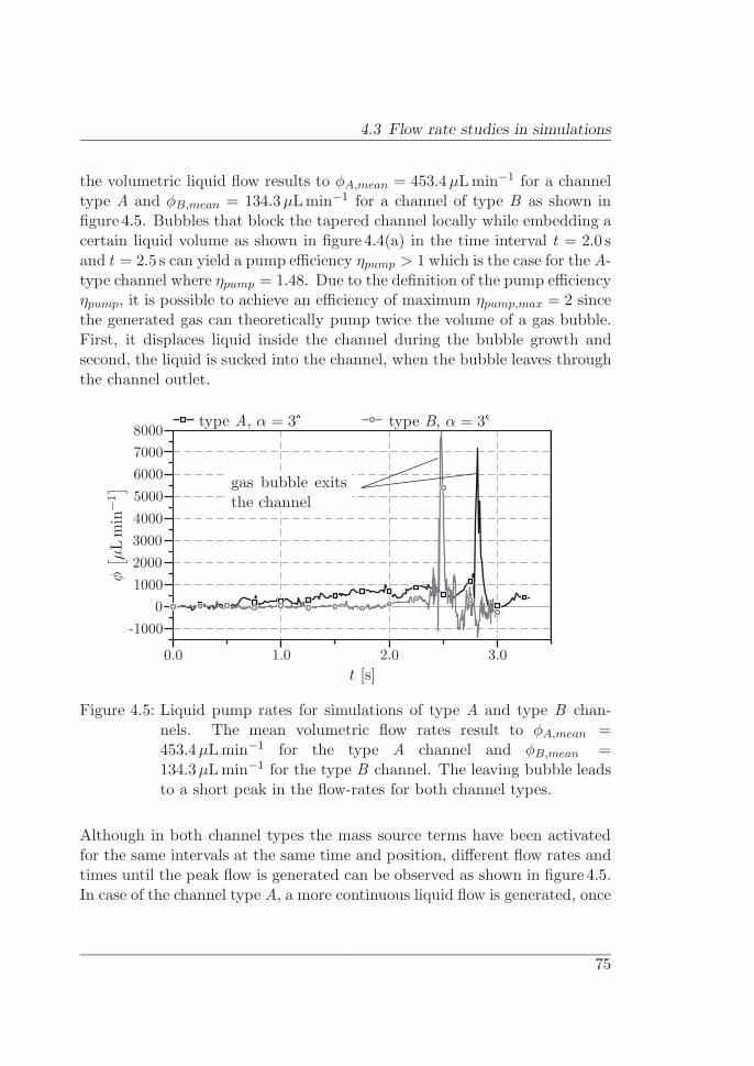
4.3 Flow rate studies in simulations
the volumetric liquid flow results to φA,mean = 453.4µL min−1 for a channeltype A and φB,mean = 134.3µL min−1 for a channel of type B as shown infigure 4.5. Bubbles that block the tapered channel locally while embedding acertain liquid volume as shown in figure 4.4(a) in the time interval t = 2.0 sand t = 2.5 s can yield a pump efficiency ηpump > 1 which is the case for the A-type channel where ηpump = 1.48. Due to the definition of the pump efficiencyηpump, it is possible to achieve an efficiency of maximum ηpump,max = 2 sincethe generated gas can theoretically pump twice the volume of a gas bubble.First, it displaces liquid inside the channel during the bubble growth andsecond, the liquid is sucked into the channel, when the bubble leaves throughthe channel outlet.
type A, α = 3� type B, α = 3�
φ[ µ
Lm
in−1
]
t [s]
-10000
10002000300040005000600070008000
0.0 1.0 2.0 3.0
gas bubble exitsthe channel
Figure 4.5: Liquid pump rates for simulations of type A and type B chan-nels. The mean volumetric flow rates result to φA,mean =453.4µL min−1 for the type A channel and φB,mean =134.3µL min−1 for the type B channel. The leaving bubble leadsto a short peak in the flow-rates for both channel types.
Although in both channel types the mass source terms have been activatedfor the same intervals at the same time and position, different flow rates andtimes until the peak flow is generated can be observed as shown in figure 4.5.In case of the channel type A, a more continuous liquid flow is generated, once
75
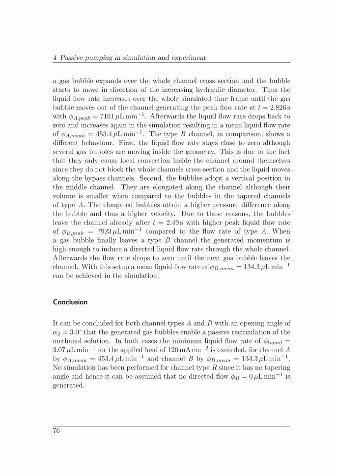
4 Passive pumping in simulation and experiment
a gas bubble expands over the whole channel cross section and the bubblestarts to move in direction of the increasing hydraulic diameter. Thus theliquid flow rate increases over the whole simulated time frame until the gasbubble moves out of the channel generating the peak flow rate at t = 2.826 swith φA,peak = 7161µL min−1. Afterwards the liquid flow rate drops back tozero and increases again in the simulation resulting in a mean liquid flow rateof φA,mean = 453.4µL min−1. The type B channel, in comparison, shows adifferent behaviour. First, the liquid flow rate stays close to zero althoughseveral gas bubbles are moving inside the geometry. This is due to the factthat they only cause local convection inside the channel around themselvessince they do not block the whole channels cross-section and the liquid movesalong the bypass-channels. Second, the bubbles adopt a vertical position inthe middle channel. They are elongated along the channel although theirvolume is smaller when compared to the bubbles in the tapered channelsof type A. The elongated bubbles attain a higher pressure difference alongthe bubble and thus a higher velocity. Due to these reasons, the bubblesleave the channel already after t = 2.49 s with higher peak liquid flow rateof φB,peak = 7923µL min−1 compared to the flow rate of type A. Whena gas bubble finally leaves a type B channel the generated momentum ishigh enough to induce a directed liquid flow rate through the whole channel.Afterwards the flow rate drops to zero until the next gas bubble leaves thechannel. With this setup a mean liquid flow rate of φB,mean = 134.3µL min−1
can be achieved in the simulation.
Conclusion
It can be concluded for both channel types A and B with an opening angle ofα2 = 3.0� that the generated gas bubbles enable a passive recirculation of themethanol solution. In both cases the minimum liquid flow rate of φliquid =3.07µL min−1 for the applied load of 120mAcm−2 is exceeded, for channel Aby φA,mean = 453.4µL min−1 and channel B by φB,mean = 134.3µL min−1.No simulation has been performed for channel type R since it has no taperingangle and hence it can be assumed that no directed flow φR = 0µL min−1 isgenerated.
76

4.4 Flow rate studies in experiments
4.4 Flow rate studies in experiments
The previously shown simulations described the fluidic behaviour in idealchannel systems with small fluidic resistors. The resulting pump efficienciesof ηpump, A = 1.74 for an A-type channel and ηpump, B = 0.26 for an B-typechannel were well above the theoretical minimum of ηpump, min = 0.01. Otherthan in the simulation the pump efficiency in the real system is expectedto differ because of contact angle hysteresis and pinning effects of the gasbubbles in the channels. In addition, the fluidic resistance in the real system isexpected to differ compared to the simulation, due to different geometry andliquid level in the connecting reservoir that works as outer loop. Furthermore,for the sake of comparability first experiments for the pumping mechanismhave been accomplished by using only one of the channels of each flow-fieldand controlled gas bubble development. The first experiment is performed todetermine the stagnation pressure of the pump and in the second experimentthe pump rate is measured in situ with a flow sensor.
The bubble development was realized with three gas inlets and a syringepump with three mounted syringes, one for each inlet. In a first test, thestagnation pressure of a type A channel has been determined by using abalance as depicted in figure 4.6, a 4M methanol solution and air as media.The volumetric gas flow rate accumulated for all three syringes was set toφair = 159µL min−1. In this setup the gas has been separated from the liquiddue to buoyancy of the gas bubbles out of the reservoir. The flow-field hasbeen mounted on a plate made out of PMMA with the three gas inlet ports.As no membrane, gas diffusion layer and recirculation loop are used, effectsdue to these parts of the fuel cell are not taken into account. The stagnationpressure the pump can withstand is determined by the mass increase at thebalance as the resulting stagnation pressure ∆P is proportional to the massincrease ∆m at the channel outlet side.
Compared to the simulation with a tapered channel and an opening angleof α2 = 3.0 � where a stagnation pressure of ∆Pmean, sim = 6.2Pa has beenachieved, the experiment shows a lower mean stagnation pressure of only∆Pmean, exp = 3.2Pa determined by the weight increase when the liquid ispumped into the reservoir at the outlet side of the channel. In the simulationthe bubbles are generated within short time intervals due to the modelling
77
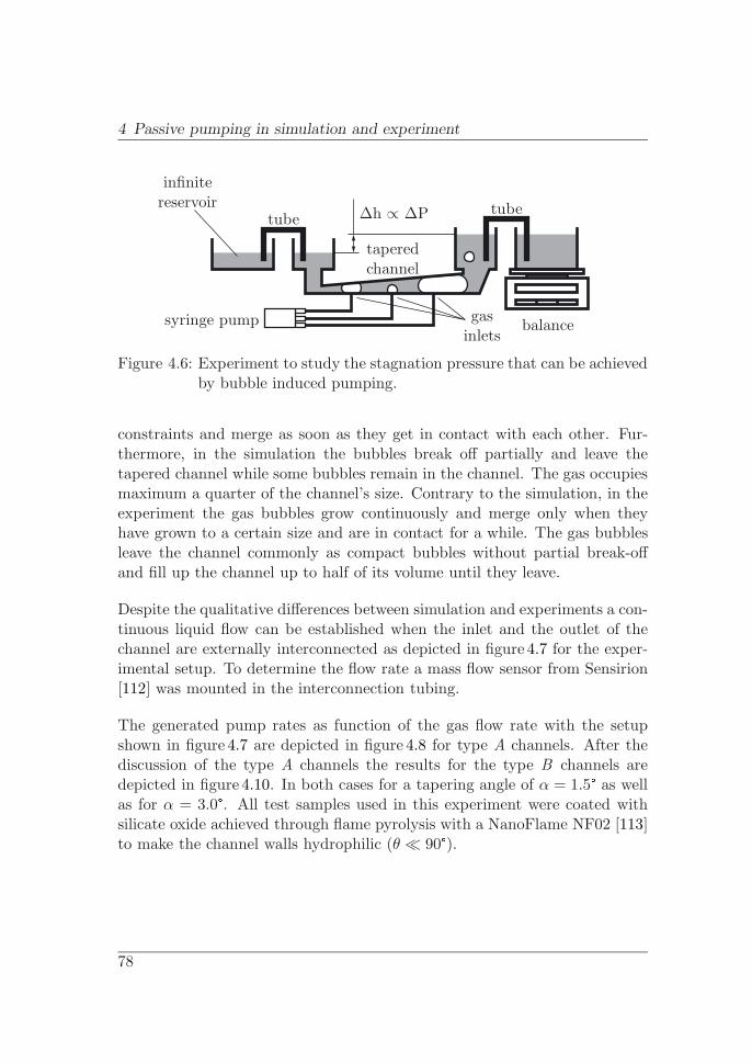
4 Passive pumping in simulation and experiment
infinitereservoir
∆h ∝ ∆P tubetube
taperedchannel
balancesyringe pump gasinlets
Figure 4.6: Experiment to study the stagnation pressure that can be achievedby bubble induced pumping.
constraints and merge as soon as they get in contact with each other. Fur-thermore, in the simulation the bubbles break off partially and leave thetapered channel while some bubbles remain in the channel. The gas occupiesmaximum a quarter of the channel’s size. Contrary to the simulation, in theexperiment the gas bubbles grow continuously and merge only when theyhave grown to a certain size and are in contact for a while. The gas bubblesleave the channel commonly as compact bubbles without partial break-offand fill up the channel up to half of its volume until they leave.
Despite the qualitative differences between simulation and experiments a con-tinuous liquid flow can be established when the inlet and the outlet of thechannel are externally interconnected as depicted in figure 4.7 for the exper-imental setup. To determine the flow rate a mass flow sensor from Sensirion[112] was mounted in the interconnection tubing.
The generated pump rates as function of the gas flow rate with the setupshown in figure 4.7 are depicted in figure 4.8 for type A channels. After thediscussion of the type A channels the results for the type B channels aredepicted in figure 4.10. In both cases for a tapering angle of α = 1.5� as wellas for α = 3.0�. All test samples used in this experiment were coated withsilicate oxide achieved through flame pyrolysis with a NanoFlame NF02 [113]to make the channel walls hydrophilic (θ � 90�).
78
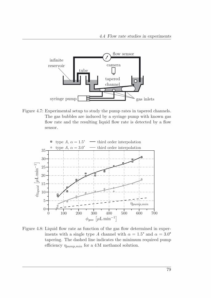
4.4 Flow rate studies in experiments
infinitereservoir camera
tube
taperedchannel
flow sensor
syringe pump gas inlets
Figure 4.7: Experimental setup to study the pump rates in tapered channels.The gas bubbles are induced by a syringe pump with known gasflow rate and the resulting liquid flow rate is detected by a flowsensor.
type A, α = 1.5� third order interpolationtype A, α = 3.0� third order interpolation
φli
quid
[ µL
min
−1]
φgas
[µL min−1
]
ηpump,min
0
5
10
15
20
25
30
35
0 100 200 300 400 500 600 700
Figure 4.8: Liquid flow rate as function of the gas flow determined in exper-iments with a single type A channel with α = 1.5� and α = 3.0�tapering. The dashed line indicates the minimum required pumpefficiency ηpump,min for a 4M methanol solution.
79

4 Passive pumping in simulation and experiment
The liquid flow rates determined for type A channels show values that are 1.5to 2.5-fold higher for the smaller tapering angle. This is due to the differentpumping modes that can be observed in the used channels with a width of3mm, a blocking mode and a non-blocking mode as sketched in figure 4.9[74, 76, 114]. In the channel with the small tapering angle the blocking modeis observed. Apart from corner flow, all liquid displaced by the growing andmoving bubbles is directed towards the channels wider end and thus does fullycontribute to the pump rate. In the non-blocking mode, as observed in thechannel with the larger tapering angle, the gas bubble does only fill a part ofthe channel and the major amount of the displaced liquid recirculates directlyaround the gas bubble. Thus the outer liquid flow rate is much smaller as inthe blocking mode. This yields that the channel width, although not variedin this work, is a further key parameter for the pumping mode, as an infinitechannel width would yield no outer liquid flow rate at all.
gas liquid gas-liquid interface
α1 = 1.5� α2 = 3.0�
3.0
mm
3.0
mm
(a) (b)
Figure 4.9: Schematic top view of moving bubbles in a tapered channel (typeA) in (a) blocking mode for a small tapering angle α1 and in (b)non-blocking mode for a large tapering angle α2
The flow rates gathered in the simulation are significantly higher than in theexperiment since in the simulation, the fluidic resistance in the outer circuit islower and the surface properties are idealized. Nevertheless the experimentsshow that the liquid flow rate is still larger than 1% of the gas flow rate. Thusthe liquid flow rate is still high enough to generate enough convection to feedmore methanol to the fuel cell than actually consumed at the correspondingbubble generation rate.
80

4.4 Flow rate studies in experiments
type B, α = 1.5� third order interpolationtype B, α = 3.0� third order interpolation
φli
quid
[ µL
min
−1]
φgas
[µL min−1
]
ηpump,min
0
0.2
0.4
0.6
0.8
1.0
1.2
1.4
0 100 200 300 400 500 600 700
Figure 4.10: Liquid flow rate as function of the gas flow determined in exper-iments with a single type B channel with α = 1.5� and α = 3.0�tapering. The dashed line indicates the minimum required pumpefficiency ηpump,min for a 4M methanol solution.
In the experiment as well as in the simulation the liquid flow rates of a typeB-channel (figure 4.10) are lower compared to a channel of type A (figure 4.8).In the experiments as depicted in figure 4.10 the resulting flow rates are evenbelow the minimum required flowrate for both tapering angles which has notbeen observed in the simulation. The main reason for this significantly lowerflow rate is based on the experimental setup. In this experiment the gasbubbles are generated at three inlets which are located directly beneath thecentral channel. In consequence the gas bubbles immediately adopt the verti-cal position in the central channel and do not block parts of the side channel.Due to this, most of the liquid recirculates around the gas bubble withoutcontributing to the flow through the reservoir. In case of the simulation aswell as in the fuel cell operation parts of the side channels are blocked andthus a higher flow rate is achieved (see figure 4.4 or figureC.3). In case ofthe type B-channel, the channel with the larger tapering angle shows thehigher liquid flow rate. As for both channel types the gas bubble completely
81
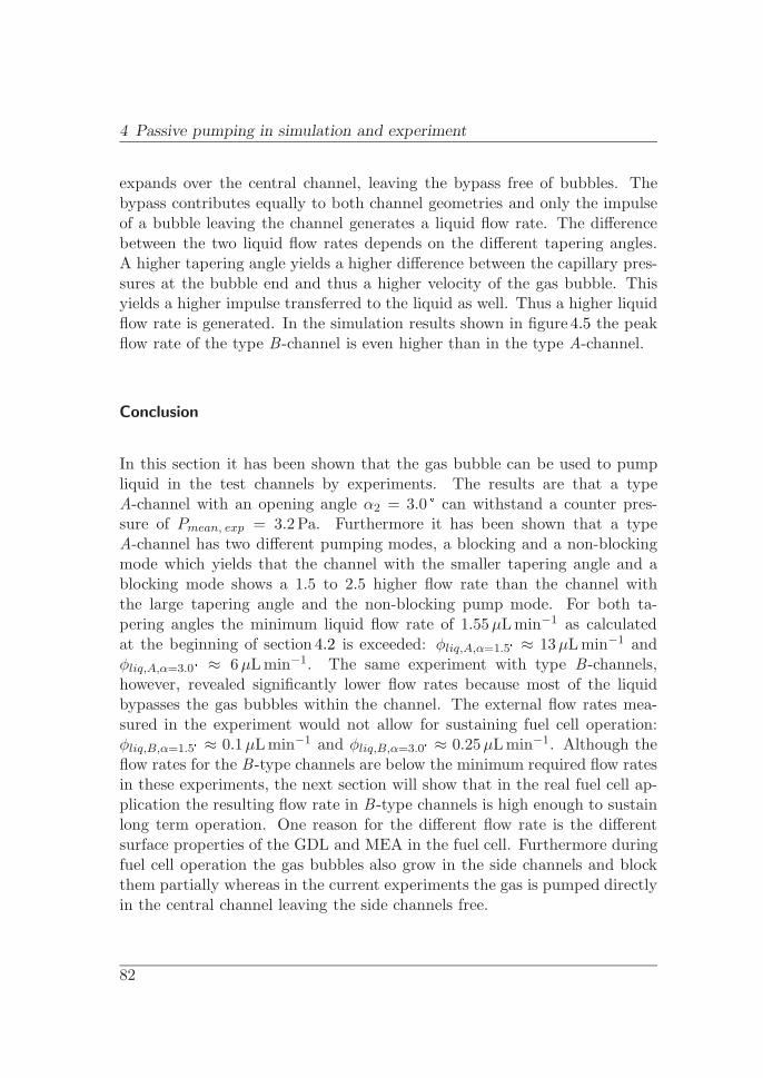
4 Passive pumping in simulation and experiment
expands over the central channel, leaving the bypass free of bubbles. Thebypass contributes equally to both channel geometries and only the impulseof a bubble leaving the channel generates a liquid flow rate. The differencebetween the two liquid flow rates depends on the different tapering angles.A higher tapering angle yields a higher difference between the capillary pres-sures at the bubble end and thus a higher velocity of the gas bubble. Thisyields a higher impulse transferred to the liquid as well. Thus a higher liquidflow rate is generated. In the simulation results shown in figure 4.5 the peakflow rate of the type B-channel is even higher than in the type A-channel.
Conclusion
In this section it has been shown that the gas bubble can be used to pumpliquid in the test channels by experiments. The results are that a typeA-channel with an opening angle α2 = 3.0 � can withstand a counter pres-sure of Pmean, exp = 3.2Pa. Furthermore it has been shown that a typeA-channel has two different pumping modes, a blocking and a non-blockingmode which yields that the channel with the smaller tapering angle and ablocking mode shows a 1.5 to 2.5 higher flow rate than the channel withthe large tapering angle and the non-blocking pump mode. For both ta-pering angles the minimum liquid flow rate of 1.55µL min−1 as calculatedat the beginning of section 4.2 is exceeded: φliq,A,α=1.5� ≈ 13µL min−1 andφliq,A,α=3.0� ≈ 6µL min−1. The same experiment with type B-channels,however, revealed significantly lower flow rates because most of the liquidbypasses the gas bubbles within the channel. The external flow rates mea-sured in the experiment would not allow for sustaining fuel cell operation:φliq,B,α=1.5� ≈ 0.1µL min−1 and φliq,B,α=3.0� ≈ 0.25µL min−1. Although theflow rates for the B-type channels are below the minimum required flow ratesin these experiments, the next section will show that in the real fuel cell ap-plication the resulting flow rate in B-type channels is high enough to sustainlong term operation. One reason for the different flow rate is the differentsurface properties of the GDL and MEA in the fuel cell. Furthermore duringfuel cell operation the gas bubbles also grow in the side channels and blockthem partially whereas in the current experiments the gas is pumped directlyin the central channel leaving the side channels free.
82

4.5 Bubble induced methanol supply of µDMFC
4.5 Bubble induced methanol supply of µDMFC
After measuring the liquid flow rate in the experiments as described in theprevious section, now it has to be verified that this principle works in a fuelcell setup. To show that self-sustaining fuel cell operation is possible, firstthe performance of a fuel cell with no bubble development is compared toone with bubble development and second a setup with a flow sensor is usedto show that the fuel recirculation flow rate φliq is larger than the minimumnecessary flow rate of φmin = 1.55µL min−1.
As a first indication for convection in a passive fuel cell setup the perfor-mance measurement of a fuel cell with bubble development and one with-out bubble development is considered. The two different operation modesshow completely different curves for the long-run measurement as depictedin figure 4.11. The setup of the experiment is described in detail in section 5.2.The characteristic curves of both cells, see figure 4.11(a), are almost identicalbut when the load of 20mAcm−2 is applied only one of the cells produces gasbubbles. Pinholes in the membrane or microscopic leakage in the core layerare likely to be the reason for the absence of visible gas bubbles in the secondfuel cell. Although pinholes or microscopic leakage seem to be the reason forthe absence of gas bubbles, the almost identical performance curves indicatethat no increased cross-over can be observed because this would lead to anasymetric power curve in figure 4.11(a).
In the long-run measurement the curve of the bubble-free fuel cell (light greyline) continuously drops from its maximum power of Pmax = 2.98mW cm−2
until after 67min under load the measurement is stopped at P = 0mW cm−2.Since there is no convection due to gas bubbles it can be assumed that onlythe methanol inside the flow-field and some minute amounts supplied bydiffusion is consumed. Subsequently the power decreases with the decreasinglocal methanol concentration at the membrane. The second curve (blackline) is typical for a passive fuel cell with bubble development. Such curvesas observed in this work can be subdivided into three characteristic intervals:
The first time interval shows a performance decreases from the initial load-free starting point of the measurement. As discussed in section 1.1 the fuel cellhas the highest methanol concentration and methanol cross-over in this part
83

4 Passive pumping in simulation and experiment
(a)
(b)
current density j[Acm−2
]
cell
voltag
eU
[mV
]
pow
erde
nsity
[ mW
cm−2
]
load for long-runmeasurements
0.00 0.01 0.02 0.03 0.040
100
200
300
400
0
1.0
2.0
3.0
4.0bubbles
bubbles
no bubbles
no bubbles
pow
erde
nsity
[ mW
cm−2
]
t [h]
long runreference
short termreference
1 2 3
4
0
1
2
3
4
5
0.5 1.0 1.5 2.0 2.5
Figure 4.11: Comparison of the characteristic performance curves (a) of twofuel cells, one with bubble development and one without as wellas (b) the power performance over time. The long time powerperformance curve can typically be subdivided in three sectionsas described in the text and marked in the figure. The powerperformance improvement (4) is typical when a water droplettears of at the cathode, increasing the air breathing area again.
84

4.5 Bubble induced methanol supply of µDMFC
of the experiment. The cross-over starts to increase when the load is appliedand then yields a reduced performance due to the increasing temperature.The higher temperature increases the methanol diffusion coefficient and leadsto a higher membrane swelling. The molecular transport caused by electro-osmotic drag which is directly related to the current density is increased[10–12, 115].
The second time interval is characterized by an almost constant level oreven increasing performance over a longer period [10]. During this time, theperformance increasing effect of decreasing methanol cross-over dominates theeffect of performance reduction due to depletion of methanol (cf. section 3.4).
During the third time interval the depletion of methanol dominates the sys-tem and yields a typical starving behaviour comparable to the characteristicsof the curve of the bubble-free cell (figure 4.11(b)) before the power drops tozero.
Although for both experiments shown in figure 4.11 the characteristic perfor-mance curves are almost identical and both experimental setups are identical,their runtime differs significantly, 67min without bubbles and 133min withbubbles. The longer run time can be attributed to the CO2 gas bubblesthat are only present in one of both fuel cells. Assuming the gas bubblesgenerate a liquid flow rate that yields a continuous fuel recirculation duringthe whole experiment, all supplied methanol is utilized at a power efficiencyof η = 7.35%. The bubble-free fuel cell only shows a power efficiency ofη = 2.9%. It has to be suspected that almost only the methanol in thechannels of the flow-field is utilized due to diffusion and convection of thesolution. The convection is caused by the increased temperature at the fuelcell membrane only.
To further study the influence of the gas bubbles and the generated flow,a setup as depicted in figure 4.12 is used. In parallel to the normal fuelcell operation, the generated convection induced by the gas bubbles can bemeasured with the flow sensor. The setup consists of the fuel cell with tworeservoirs mounted on top. The two reservoirs are connected with each otherwith a tube and the Sensirion [112] flow sensor. As the methanol solution hasto be transferred through the tube and flow sensor, a fluidic resistor is addedto the recirculation loop when compared to a system with a single reservoir.
85

4 Passive pumping in simulation and experiment
By using a single reservoir one can assume to have very small fluidic resistancethat can be neglected. By using the setup as depicted in figure 4.12, the flowrate generated by the gas bubbles can be measured. At the same time, ahigher fluidic resistance of the system because of the additional tubes has tobe accepted.
air
methanolsolution
risingCO2-bubble
anode currentcollector
cathode cur-rent collector
membrane and gasdiffusion layers
flow field
upper mount-ing plate
lower mount-ing plate
φflow sensor
Figure 4.12: Experimental setup with two separate reser-voirs interconnected via a flow sensor todetermine the pump rate due to bubblemovement.
The experimental setup described above has been used in fuel cell experimentsfor channels of the types R, A and B. In comparison to the experimentsof single channel, the fuel cell consists of three parallel channels. One ofthe channel walls is formed by the gas diffusion layer and the PMMA flowfield with a tapering angle of α = 3� has a contact angle θ � 0�. At aload of I = 20mA cm−2 mean flow rates of φR = −24.8µL min−1, φA =20.4µL min−1 and φB = 8.2µL min−1 have been measured which correspondto pump efficiencies of ηpump,R = 16%, ηpump,A = 13% and ηpump,B = 5%.The corresponding curves of the flow rates as an excerpt of 1min are shownin figure 4.13.
With a flow rate of φR = −24.8µL min−1 the type R channel has the highestabsolute value for the flow which is depicted opposite to the flow of the othersamples. By theory one would expect no or only little flow in this kind ofchannel design since the bubbles can randomly leave the flow field channelsthrough both ends. But in case of a crack in the gas diffusion layer a piningbarrier can be created acting as a ”check valve“, leaving only one direction
86
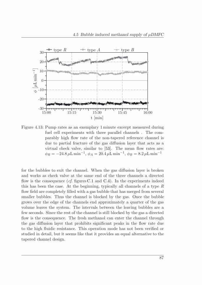
4.5 Bubble induced methanol supply of µDMFC
type R type A type B
φ[ µ
Lm
in−1
]
t [min]
-30
-20
-10
0
10
20
30
15:00 15:15 15:30 15:45 16:00
Figure 4.13: Pump rates as an exemplary 1minute excerpt measured duringfuel cell experiments with three parallel channels . The com-parably high flow rate of the non-tapered reference channel isdue to partial fracture of the gas diffusion layer that acts as avirtual check valve, similar to [53]. The mean flow rates are:φR = −24.8µL min−1, φA = 20.4µL min−1, φB = 8.2µL min−1
for the bubbles to exit the channel. When the gas diffusion layer is brokenand works as check valve at the same end of the three channels a directedflow is the consequence (cf. figuresC.1 and C.4). In the experiments indeedthis has been the case. At the beginning, typically all channels of a type Rflow field are completely filled with a gas bubble that has merged from severalsmaller bubbles. Thus the channel is blocked by the gas. Once the bubblegrows over the edge of the channels end approximately a quarter of the gasvolume leaves the system. The intervals between the leaving bubbles are afew seconds. Since the rest of the channel is still blocked by the gas a directedflow is the consequence. The fresh methanol can enter the channel throughthe gas diffusion layer that prohibits significant peaks in the flow rate dueto the high fluidic resistance. This operation mode has not been verified orstudied in detail, but it seems like that it provides an equal alternative to thetapered channel design.
87

4 Passive pumping in simulation and experiment
In a tapered channel (type A) the mean flow rate of φA = 20.4µL min−1 hasbeen measured. In comparison to the results of the type R flow field, the flowrate shows an irregular curve form. It increases continuously over a periodof several seconds from φmin = 16µL min−1 to φmax = 25µL min−1. Thenit drops down within a few seconds and starts to increase again. Basicallythe bubble growth in the channels is similar to type R channels, the bubblesstart to grow in a random distribution inside the channel and merge whenthey get into contact with each other until they are large enough to block thewhole channel cross-section. By the tapering, their further growth is directedtowards the wider channel part. Thus a directed positive flow is generated.Once the bubble has grown to the outlet either the complete bubble leavesthe channel or a large part of it tears of and up to a third of it stays inthe channel (cf. figuresC.2 and C.4). Likewise to the simulation shown infigure 4.5 the flow rate decreases after the bubble left the channel. Sincethree of the channels act in parallel, there is a superposition of the flow rategenerated in each of the three channels. This yields a positive flow that isalways larger than φ ≥ 16µL min−1 in this experimental setup.
The B-type channel shows a significantly lower flow rate when compared tothe other two channel types. With a mean flow rate of φB = 8.2µL min−1 itis only approximately half the flow rate of the other channels. Neverthelessthe flow rate is still high enough to achieve sufficient fuel convection for longterm operation. The characteristics of the curve shows a wave form within arange of 7µL min−1 ≤ φB ≤ 11µL min−1. The lower flow rate is due to thepossible liquid flow around the bubbles through the bypass channels. The gasbubbles that develop in the bypass channels first move towards the middlechannel, when they have grown to a certain size. Since the surface roughnessof the gas diffusion layer pins the bubbles, their residence time is longer thanin the simulation. Thus they grow to a bigger size and partially block theside channels, increasing the fluidic resistance. This is the main reason whythe ratio of φB/φA is 0.41 in the experiments and only 0.3 in the simulation,where the influence of the surfaces is neglected. Due to the channel geometryand the smaller bubbles volume the events of bubble emission are every 10 sto 15 s (cf. figuresC.3 and C.4). The higher emission rate and the smallerbubble volumes when compared to the type A channel yields a smoothercurve of the flow rate.
88

4.5 Bubble induced methanol supply of µDMFC
Conclusion
Finally, it has successfully been demonstrated in this section that once bub-bles are generated in a fuel cell with type A-channels and type B-channels,the methanol solution is pumped through the fuel cell to sustain long termfuel cell operation. The measured mean recirculation flow rates of φA =20.4µL min−1 (ηpump,A = 13%) and φB = 8.2µL min−1 (ηpump,B = 5%) aresignificantly larger than the minimum flow rate φmin = 1.55µL min−1 that isrequired to sustain fuel cell operation. Furthermore it has been demonstratedthat if no gas bubbles are generated, no fuel recirculation occurs either. Inthis case the fuel cell power performance decreases continuously once theexperiment is started since only the methanol next to the membrane is uti-lized. Although expected not to recirculate the methanol solution, it hasbeen shown that type R-channels are able to pump the liquid. The measuredaverage flow rate of φR = 24.8µL min−1 (ηpump,R = 16%) is sufficient forcontinuous supply. The deformed gas diffusion layer and pinning effects atthe transition between the gas diffusion layer and the anode current contacthave been identified as reasons for the directed gas bubble removal in thischannel type. The deformation and the pinning effect yield an effect similarto a check-valve for the gas bubbles.
89

5 Passive fuel cell designs driven by capillary forces
In comparison to the previously discussed active fuel cells in chapter 3 thischapter focuses on a completely passive fuel cell setup. It comprises theapplication of the bubble induced pumping method of chapter 4 in the fuelcell. Therefore, the flow field design and the experimental setup as usedin this chapter are introduced first. In the experimental part, the long runmeasurements and its results as well as the stability of the power output are ofspecial interest. Furthermore the scaling behaviour of the reservoir contentsversus the run time is studied and possible improvements to increase theruntime while using higher methanol concentrations.
5.1 Passive flow field design / Experimental setup
While the flow fields used for the active fuel cell setup had a tube at theinlet and outlet for the fuel supply the flow field used for the experimentsin this chapter are connected to the reservoir via a slotted hole as shown infigure 5.1. The fuel feed and outlet are the only constructional differences ofthe flow fields. The channels themselves are of the same dimensions. Whenobserved in a cross-sectional view, the flow field is immersed in the reservoiras depicted in figure 5.2. Thus, the maximum run time of the fuel cell isdelimited by the reservoir in terms of volume and methanol concentration.Once the methanol solution has been pipetted into the reservoir, it has beencovered with Parafilm M� [116] to reduce evaporation. The method to ac-quire the experimental data is identical to the method previously describedin section 3.3.
91
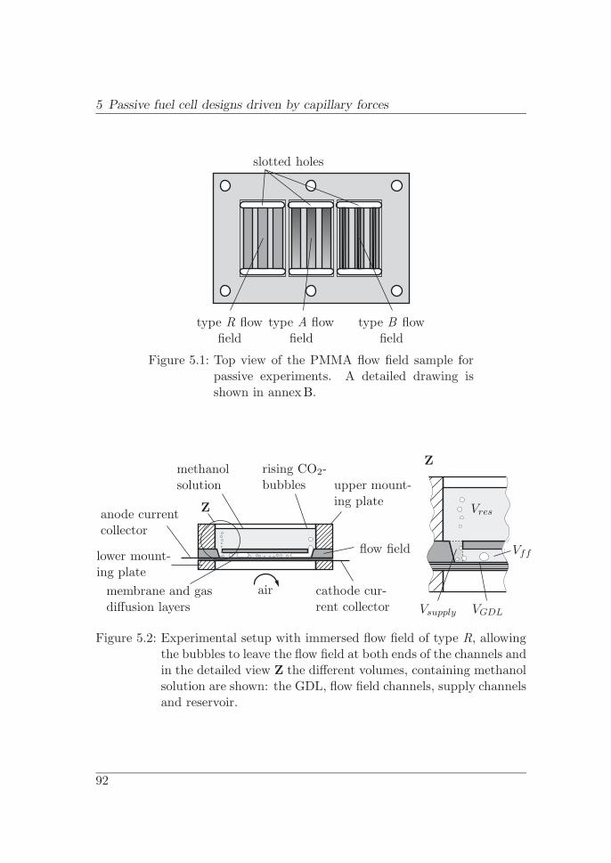
5 Passive fuel cell designs driven by capillary forces
slotted holes
type R flowfield
type A flowfield
type B flowfield
Figure 5.1: Top view of the PMMA flow field sample forpassive experiments. A detailed drawing isshown in annexB.
air
methanolsolution
rising CO2-bubbles
anode currentcollector
cathode cur-rent collector
membrane and gasdiffusion layers
flow field
upper mount-ing plate
lower mount-ing plate
Z
Z Vres
Vff
Vsupply VGDL
Figure 5.2: Experimental setup with immersed flow field of type R, allowingthe bubbles to leave the flow field at both ends of the channels andin the detailed view Z the different volumes, containing methanolsolution are shown: the GDL, flow field channels, supply channelsand reservoir.
92

5.1 Passive flow field design / Experimental setup
Provided chemical energy by fuel cell volumes
In the studies of the passive fuel cells it is of special interest whether all theprovided methanol is utilized during the experiment and a fuel recirculationis achieved. Therefore, the energy contents of each volume at the fuel cellsanode side is calculated. The different volumes are the gas diffusion layerVGDL with a porosity of 50 %, the flow field channels Vff , the fuel supplyVsupply and the reservoir Vres. With a given volume of the methanol solutionV = 2.0mL and concentration cMeOH = 4mol L−1 the resulting values forthe different parts of the assembly are given in table 5.1. These values areused to compare the resulting electrical energy generated during the fuelcell operation with the energy contents of the different volumes. When theresulting energy output during one experiment exceeds the energy providedin the flow field and the gas diffusion layer, a further proof for a passivetransport of the fuel is given.
Table 5.1: Volumes of the different parts of the fuel cells anode side, the gasdiffusion layer, flow field, supply channels and reservoir. For eachvolume the corresponding chemical energy Wc for 2.0mL of a 4Mmethanol solution is given. The total energy in the solution isWc,2 mL,4 M = 750 J.
Cell type VGDL [mL] Vff [mL] Vsupply [mL] Vres [mL]Wc,GDL [J] Wc,ff [J] Wc,supply [J] Wc,res [J]
R 0.05 0.18 0.36 1.4120 68 135 527
A 1.5� 0.05 0.19 0.36 1.3920 72 135 523
A 3.0� 0.05 0.24 0.36 1.3520 89 135 506
B 1.5� 0.05 0.1 0.36 1.4920 37 135 558
B 3.0� 0.05 0.11 0.36 1.4720 42 135 553
93

5 Passive fuel cell designs driven by capillary forces
5.2 Experiments with capillary fuel supply
In the previous chapter 4 it has been shown that the gas bubbles can be usedas an intrinsic pump for the fuel delivery in the fuel cell. Using this fuel deliv-ery method, the different channel types are now studied regarding their per-formance. First, the reference channel (type R-channel) is studied. Second,the performance of type A-channels and B-channels with different openingangles are compared. Finally, two different options for run time extension arestudied, the enlargement of the fuel cell reservoir and the re-dosage of highconcentrated methanol into the reservoir at certain time intervals.
Capillary fuel supply for reference cell
The layout of R-type channels are non-tapered and thus this system is ex-pected not to pump any liquid. However, it is well known that changes ofthe surface, e.g. material changes, or geometry changes can influence the be-haviour of a moving capillary interfaces, e.g. Ducree et al [117], and thusbubble movement.
As already discussed in section 4.5 the transition between the anode currentcollector and the gas diffusion layer which in addition has been partiallyfractured acts as a virtual check-valve like proposed as system design byMeng et al [53]. Due to the fractured gas diffusion layer the growing gasbubbles can not exit through both sides of the channel ends and a directedflow is established. The runtime and power performance with a 4M methanolsolution and a volume of 2.0mL are depicted in figure 5.3. The providedchemical energy of this setup is Wc = 750 J and the achieved electrical energyoutput is Eel = 64J.
By comparing the mean power performance of Pmean = 2.5mWcm−2 at anefficiency of this fuel cell ηR = 8% with the mean performance achieved inthe active reference experiment (section 3.4) of Pref,lrr = 1.5mWcm−2. Theperformance improvement is about 1.7× against the reference.
94
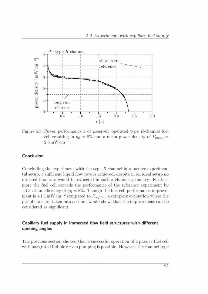
5.2 Experiments with capillary fuel supply
type R-channel
pow
erde
nsity
[ mW
cm−2
]
t [h]
long runreference
short termreference
0
1
2
3
4
5
0.5 1.0 1.5 2.0 2.5 3.0
Figure 5.3: Power performance a of passively operated type R-channel fuelcell resulting in ηR = 8% and a mean power density of Pmean =2.5mWcm−2.
Conclusion
Concluding the experiment with the type R-channel in a passive experimen-tal setup, a sufficient liquid flow rate is achieved, despite in an ideal setup nodirected flow rate would be expected in such a channel geometry. Further-more the fuel cell exceeds the performance of the reference experiment by1.7× at an efficiency of ηR = 8%. Though the fuel cell performance improve-ment is +1.1mWcm−2 compared to Pref,lrr, a complete evaluation where theperipherals are taken into account would show, that the improvement can beconsidered as significant.
Capillary fuel supply in immersed flow field structures with differentopening angles
The previous section showed that a successful operation of a passive fuel cellwith integrated bubble driven pumping is possible. However, the channel type
95

5 Passive fuel cell designs driven by capillary forces
R is by its layout not dedicated to pump, whereas the type A and B-channelsare expected to pump due to their design. Their ability to pump liquid hasbeen proven and discussed in chapter 4. By using the same experimentalsetup as depicted in figure 5.2 with 2.0mL of a 4M methanol solution, thesechannels are studied now in a flow field with three parallel channels anda GDL as bottom surface. Furthermore the influence of different taperingangles of α1 = 1.5� and α2 = 3.0� are studied.
Figure 5.4 (a) shows the power performance of the type A-channels with dif-ferent tapering angles. Both fuel cells have a runtime of over 2.5 hours anda power output of Eel,A,1.5� = 64J for the tapering angle of α1 = 1.5�and Eel,A,3.0� = 54J for the tapering angle α2 = 3.0�. During the experi-ment the mean power output of both fuel cells is at values of Pmean,A,1.5� =2.3mWcm−2 and Pmean,A,3.0� = 1.9mWcm−2. These mean values are afactor of 1.5× for α1 and 1.27× for α2 higher than the long run referencewith Pref = 1.5mWcm−2. Furthermore efficiencies of ηA,1.5� = 8% andηA,3.0� = 7% have been achieved. The performance of the fuel cell with thesmall tapering angle shows a higher mean power output but also a runtimethat is shorter than the runtime of the fuel cell with the higher opening an-gle. According to the measurements of the liquid flow rate in the previouschapter, both tapering angles show a flow rate high enough for sufficient fuelrecirculation which is now proven in a fuel cell setup as well.
The long term performance curves of the type B-channel fuel cells with thetwo opening angles α1 and α2 are depicted in figure 5.4 (b). The runtime ofthe two cells is around 2.5 hours. For the opening angle α1 the power outputis Pmean,B,1.5� = 2.7mWcm−2. This exceeds the long run reference of theactively fuel cells by a factor of 1.8. This fuel cell shows the best efficiency ofthe experiments discussed in this section of ηB,1.5� = 10%. In comparison tothis performance curve, the power output of the type B-channel with α2 con-tinuously decreases over its runtime. The reason for the continuous decreaseof the power density output during the experiment could not be determined..Nevertheless, the mean power output of Pmean,B,3.0� = 1.8mWcm−2 at an ef-ficiency of ηB,3.0� = 6% is still 1.2× larger than the efficiency of the referencefuel cell.
96

5.2 Experiments with capillary fuel supply
(a)
(b)
type A, α1 = 1.5� type A, α2 = 3.0�
type B, α1 = 1.5� type B, α2 = 3.0�
pow
erde
nsity
[ mW
cm−2
]po
wer
dens
ity
[ mW
cm−2
]
t [h]
t [h]
long runreference
long runreference
short termreference
short termreference
0
0
1
1
2
2
3
3
4
4
5
5
0.5
0.5
1.0
1.0
1.5
1.5
2.0
2.0
2.5
2.5
3.0
3.0
Figure 5.4: Comparison of passive fuel cell operation in type A-channels (a)and type B-channels (b) at different channel tapering angles α1 =1.5% and α2 = 3.0%. The efficiencies of the type A-channels areηA,1.5� = 8% and ηA,3.0� = 7% while for the type B-channels areηB,1.5� = 10% and ηB,3.0� = 6%.
97

5 Passive fuel cell designs driven by capillary forces
Conclusion
In the previous section it is proven that for both channel designs (A and B)and tapering angles (α1 = 1.5� and α2 = 3.0�) a reliable and almost constantpower output over 1.5 h at a total runtime of more than 2.5 h is possible withbubble induced recirculation of methanol. Thereby the mean power densitiesof all four fuel cell setups are 1.2× to 1.8× higher than the efficiency of thereference fuel cell. The mean power densities for both fuel cells with thetapering angle α1 are in the same order of magnitude or higher than thepassively operated type R-channel fuel cell and their efficiencies are about8%.
The mean power density as well as the efficiency for the B-type channel withan opening angle of α2 = 1.5� shows the highest value with Pmean,B,1.5� =2.7mWcm−2 and ηB,1.5� = 10%. The same channel type with the taperingangle α1 = 3.0� has the lowest values for power density and efficiency but isstill better than mean power density Pref of the reference experiments.
But same as for the active system, no significant differences between thedifferent channel types can be observed. This includes the R-type channelwhere also a flow rate can be measured although the flow direction is notgeometrically defined like in the A and B-type channels. As the runtime ofonly 2.5 hours is not long enough for portable systems it needs to be enhanced.Thus to increase the runtime, either the fuel volume has to be increased,which will be discussed in the following part of section 5.2 or pure methanolhas to be re-dosed into the reservoir as discussed in the last part of section 5.2.
Long term fuel cell operation with capillary fuel supply
One option to extend the runtime of a passive fuel cell is by increasing thevolume of methanol solution provided. For this reason a larger reservoirhas been mounted on the flow field with an α = 3� tapering angle. Thislarger reservoir has been used for two different volumes of methanol solution:3.1mL and 9.1mL. These two volumes have been chosen to study how theruntime of the fuel cell depends on the provided methanol volume and if therecirculation of fuel is stable over a longer period of time.
98

5.2 Experiments with capillary fuel supply
Since all types of channel designs (R, A and B) proved to be pumping themethanol solution all three types were used in this experiment. The long termperformance curves of all three channel types for 9.1mL of a 4M methanolsolution are shown in figure 5.5. All of the measured fuel cells show a runtimeof more than 15 hours and a constant or slightly decreasing power output over10 hours with an efficiency of ηR = 12%, ηA,3.0� = 10% and ηB,3.0� = 11%.When compared to the efficiencies of the previous experiment with 2.0mLreservoir filling volume, the efficiency increases by 3% which can be explainedby the longer period of constant power output relative to the run-in and run-out periods of the fuel cell.
type R type A type B
pow
erde
nsity
[ mW
cm−2
]
t [h]
long runreference
short termreference
0
1
2
3
4
5
2.5 5.0 7.5 10.0 12.5 15.0 17.5
Figure 5.5: Long term performance measurements with a passive fuel cellsetup for the channel types R, A and B and 9.1mL of a 4Mmethanol solution in the reservoir. The mean energy densitiesand efficiencies are:Pmean,R = 2.4mWcm−2 with ηR = 12%Pmean,A,3.0� = 1.9mWcm−2 with ηA,3.0� = 10%Pmean,B,3.0� = 2.2mWcm−2 with ηB,3.0� = 11%
This experiment verifies the recirculation of the methanol since for all threechannel types more electrical energy is generated compared to the chemicalenergy provided in the gas diffusion layer VGDL, the flow field Vff and thesupply channels Vsupply. As listed in table 5.1 the chemical energy provided
99

5 Passive fuel cell designs driven by capillary forces
in these three fuel cell parts equates to Wc,R = 223 J for the R-type channel.In case no fuel is recirculated, the electrical energy generated in the experi-ment can not exceed this value. But the generated electrical energy in thisexperiment was Eel,R = 405 J and thus chemical energy has been transportedto the membrane by gas bubble induced pumping. The same comparisonwas done for the two other channel types. For the A-type channel flow fieldthe chemical energy provided in VGDL + Vff + Vsupply was Wc,A,3.0� = 244 Jand the generated electrical energy was Eel,A = 336 J. In the B-type channelflow fields, the values were Wc,B,3.0� = 197 J for VGDL + Vff + Vsupply andEel,B = 360 J for the generated electrical energy.
type R type A type B
t[h
]
reservoir contents [mL]
0.0
2.5
5.0
7.5
10.0
12.5
15.0
17.5
0 1 2 3 4 5 6 7 8 9 10
Figure 5.6: Linear scaling of the run time as function of the reservoir con-tents for the channel types R, A and B. The linearity indicates acomplete convective mixing due to the bubble induced pumping.Linear fitting of the curves yield:trun,R = 1.861 · V4 M, MeOH, sol − 1.204trun,B = 1.899 · V4 M, MeOH, sol − 1.087trun,B = 1.798 · V4 M, MeOH, sol − 1.214
In addition to the 2.0mL and 9.1mL reservoir filling volume the same exper-iment has been made for a volume of 3.1mL as well. The runtime of thesecells is about 4.5 hours as shown in figure 5.6 where the runtime of the fuel
100

5.2 Experiments with capillary fuel supply
cells is plotted against the reservoir filling volume of the 4M methanol solu-tion. This data indicates a linear correlation between the filling volume andthe runtime of the fuel cell. It shows that a certain amount of the providedmethanol solution can be indicated as losses since the linear fit has an offsetto the origin. Possible reasons for these losses, although not further studiedin this work, are the cross-over and evaporation from the reservoir.
Since there is a linear correlation between filling volume and runtime of thefuel cells, the efficiencies can be expected to be almost constant for all threechannel types during the variation of the filling volume. In table 5.2 the elec-trical energy Eel that has been provided by the system during the experimentsas well as the efficiencies are listed. It can be observed that the efficiencies ofall three types of fuel cells increase for a higher fuel volumes in the reservoir.The average values of the efficiencies are ηmean,R = 11%, ηmean,A,3.0� = 10%and ηmean,B,3.0� = 9%. In addition, the mean power output of Pmean,R =2.4mWcm−2, Pmean,A,3.0� = 1.9mWcm−2 and Pmean,B,3.0� = 2.2mWcm−2
are more than 1.2× higher than Pref = 1.5mWcm−2.
Table 5.2: Mean power densities of the system for a 4M methanol solu-tion at different reservoir filling volumes VMeOH,sol. The ef-ficiency η is calculated with respect to the theoretically pro-vided chemical energy of Wc = 750 J for VMeOH,sol = 2.0mL,Wc = 1163 J for VMeOH,sol = 3.1mL and Wc = 3414 J forVMeOH,sol = 9.1mL.
Channel Pmean [mWcm−2] and η [%] Averagetype at VMeOH,sol of efficiency η [%]
2.0mL 3.1mL 9.1mL
R 2.5 3.0 2.4η = 8 η = 13 η = 12 ηmean = 11
A, α2 = 3.0� 1.9 2.7 1.9η = 7.2 η = 12 η = 10 ηmean,A,3.0� = 10
B, α2 = 3.0� 1.8 2.6 2.2η = 6 η = 10 η = 11 ηmean,B,3.0� = 9
101

5 Passive fuel cell designs driven by capillary forces
Conclusion
The long term experiments with a run time of over 15 hours proofs that thefuel recirculates inside the fuel cell. This is proven by the generated electricalenergy during these experiments since fuel recirculation is required to gener-ate more electrical energy than provided in the gas diffusion layer, the flowfield and the fuel supply only (see table 5.1). In case, there is no recirculationonly the chemical energy provided in these volume close to the membranecan be utilized. For example in the R-type flow field, the generated electricalenergy was Eel,R = 405 J while the chemical energy in the gas diffusion layer,the flow field and the supply channels equates Wc,R = 223 J. Furthermore thelinear correlation of the run time versus the reservoir contents indicates thatthe amount of fuel is limiting the runtime of the fuel cell. Even the efficiencyof the long term experiments is increased by more than 3% compared to theexperiments with 2.0mL, e.g. for the R-type channel from ηR,2.0 mL = 8% toηR,9.1 mL = 12% for the experiment with 9.1mL methanol solution. It showsthat this type of fuel cell as studied in this work is better suited for continuouslong term operation. These experiments proof that the fuel recirculation bygas bubbles is a stable process as the fuel cells run with similar performanceover several hours.
Long term fuel cell operation with capillary fuel supply and re-dosage ofconcentrated methanol at intervals
As already shown for the active pumping fuel cell setup in section 3.4 discon-tinuous pumping increases the efficiency of the active cell. A similar approachcan be used for the passive fuel cell setup where pure methanol is re-dosedafter a certain period into the reservoir.
Compared to the approach studied in the previous section, the reservoir sizecan be reduced due to the higher energy density of pure methanol. Only avalve that opens periodically in a system layout has to be implemented. Butin comparison to the continuously or discontinuously pumped active systemonly the methanol concentration in the reservoir is increased and the mixingand recirculation of the solution is achieved by the passive, bubble inducedpumping.
102

5.2 Experiments with capillary fuel supply
type R type A type B
pow
erde
nsity
[ mW
cm−2
]
t [h]
long runreference
short termreference
methanolre-dosage
0
1
2
3
4
5
1 3 4 4 5 6
Figure 5.7: Long term experiment with a passive fuel cell setup with taperingangle of α = 3.0� and re-dosage of pure methanol after 60min ofoperation. The initial start volume was 3mL of 4M methanol.After 60min 162µL of pure methanol are re-dosed into the reser-voir. The mean energy densities and efficiencies are:Pmean,R = 2.4mWcm−2 with ηR = 6%Pmean,A,3.0� = 2.2mWcm−2 with ηA,3.0� = 6%Pmean,B,3.0� = 2.3mWcm−2 with ηB,3.0� = 6%
The experiment starts with a 4M methanol solution at a reservoir fill volumeof 3.0mL. After 60min 162µL methanol is pipetted into the reservoir toincrease the methanol concentration in the reservoir again. The performancecurves achieved during this experiment for all three types of fuel cells is shownin figure 5.7, where the tapered channels have an opening angle of α2 = 3.0�.All three curves start at the level of the short term reference and first showa declining curve. Then the curve starts to increase until the methanol isdosed into the reservoir. As the volume that is pumped through the fuel cellconsists of the flow field and the reservoir, the curve form is stretched whencompared to the active re-dosage with pumping at intervals (see figure 3.14).Pure methanol has been re-dosed three times in this experiment and thecurve form is basically the same during each period. However, it is obvious
103
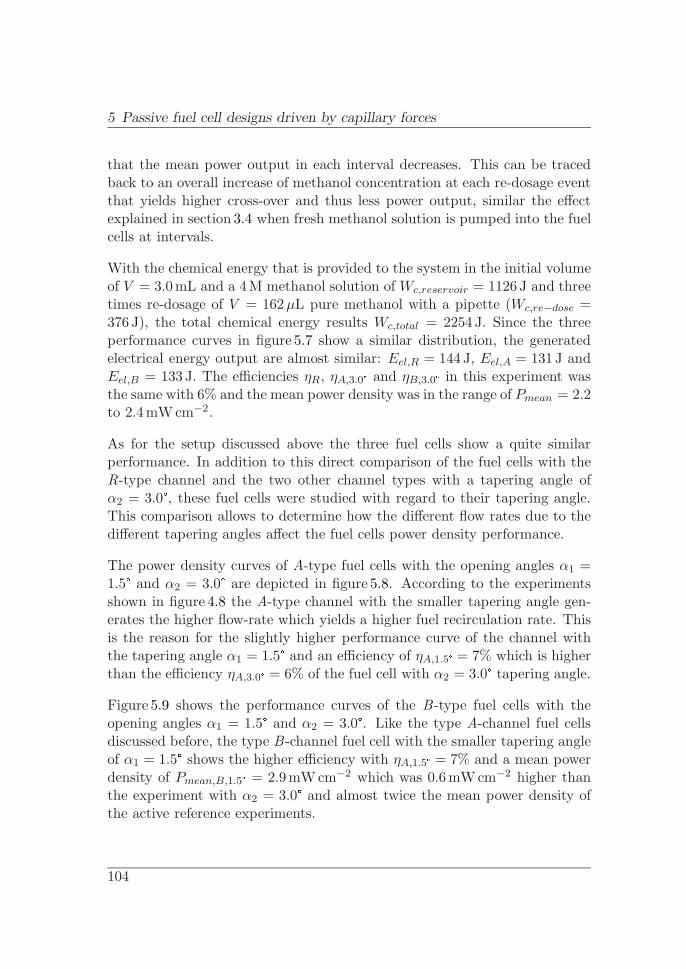
5 Passive fuel cell designs driven by capillary forces
that the mean power output in each interval decreases. This can be tracedback to an overall increase of methanol concentration at each re-dosage eventthat yields higher cross-over and thus less power output, similar the effectexplained in section 3.4 when fresh methanol solution is pumped into the fuelcells at intervals.
With the chemical energy that is provided to the system in the initial volumeof V = 3.0mL and a 4M methanol solution of Wc,reservoir = 1126 J and threetimes re-dosage of V = 162µL pure methanol with a pipette (Wc,re−dose =376 J), the total chemical energy results Wc,total = 2254 J. Since the threeperformance curves in figure 5.7 show a similar distribution, the generatedelectrical energy output are almost similar: Eel,R = 144 J, Eel,A = 131 J andEel,B = 133 J. The efficiencies ηR, ηA,3.0� and ηB,3.0� in this experiment wasthe same with 6% and the mean power density was in the range of Pmean = 2.2to 2.4mWcm−2.
As for the setup discussed above the three fuel cells show a quite similarperformance. In addition to this direct comparison of the fuel cells with theR-type channel and the two other channel types with a tapering angle ofα2 = 3.0�, these fuel cells were studied with regard to their tapering angle.This comparison allows to determine how the different flow rates due to thedifferent tapering angles affect the fuel cells power density performance.
The power density curves of A-type fuel cells with the opening angles α1 =1.5� and α2 = 3.0� are depicted in figure 5.8. According to the experimentsshown in figure 4.8 the A-type channel with the smaller tapering angle gen-erates the higher flow-rate which yields a higher fuel recirculation rate. Thisis the reason for the slightly higher performance curve of the channel withthe tapering angle α1 = 1.5� and an efficiency of ηA,1.5� = 7% which is higherthan the efficiency ηA,3.0� = 6% of the fuel cell with α2 = 3.0� tapering angle.
Figure 5.9 shows the performance curves of the B-type fuel cells with theopening angles α1 = 1.5� and α2 = 3.0�. Like the type A-channel fuel cellsdiscussed before, the type B-channel fuel cell with the smaller tapering angleof α1 = 1.5� shows the higher efficiency with ηA,1.5� = 7% and a mean powerdensity of Pmean,B,1.5� = 2.9mWcm−2 which was 0.6mWcm−2 higher thanthe experiment with α2 = 3.0� and almost twice the mean power density ofthe active reference experiments.
104

5.2 Experiments with capillary fuel supply
α = 1.5� α = 3.0�
pow
erde
nsity
[ mW
cm−2
]
t [h]
long runreference
short termreference
0
1
2
3
4
5
1 3 4 4 5 6
Figure 5.8: Comparison of long term experiment with a passive fuel cell setupand re-dosage of pure methanol in type A-channels where themean power density and the efficiencies were:Pmean,A,1.5� = 2.6mWcm−2 with ηA,1.5� = 7%Pmean,A,3.0� = 2.2mWcm−2 with ηA,3.0� = 6%
α = 1.5� α = 3.0�
pow
erde
nsity
[ mW
cm−2
]
t [h]
long runreference
short termreference
0
1
2
3
4
5
1 3 4 4 5 6
Figure 5.9: Comparison of long term experiment with a passive fuel cell setupand re-dosage of pure methanol in type B-channels where themean power density and the efficiencies were:Pmean,B,1.5� = 2.9mWcm−2 with ηB,1.5� = 7%Pmean,B,3.0� = 2.3mWcm−2 with ηB,3.0� = 6%
105

5 Passive fuel cell designs driven by capillary forces
When comparing the performance curves for the active setup that has beenpumped at intervals and the passive setup with manual methanol re-dosage,it can be observed that the curve form of the run out shows the same char-acteristics (cf. figure 5.10). The performance of the discontinuously pumpedfuel cell instantaneously decreases when the fresh methanol is flushed into theflow field while the performance decrease of the re-dosed fuel cell is delayedas the higher concentrated methanol is slowly pumped into the flow field.While the methanol concentration is fixed to the 2M solution for the activesystem, the methanol concentration in the passive system is very likely higherthan 2M after the re-dosage. Thus a higher cross-over results in a strongerperformance decrease for the passive fuel cell. For both fuel cells, the perfor-mance starts to increase again over the run-time as the methanol solution isutilized and the concentration decreases until almost all methanol is used up.What differs for the two performance curves is the total run-time after thelast pumping interval/re-dose of methanol. The active system delivers powerfor 33minutes while the passive system has a run-out-time of 110minutes.This difference is due to the different volumes of methanol solution and theability of the passive system to recirculate inside the fuel cells flow field andreservoir. The active system does only provide the chemical energy that isstored in the volume of the methanol solution inside the flow field and the dis-tribution channels. In addition the recirculation of methanol inside the flowfield is obstructed by the gas bubbles that first block the flow field channelsand can only exit through the outlet channel. During this time, a part of themethanol solution is pushed out of the fuel cell by the exiting gas bubbles.In contrast to this, the gas bubbles lead to a better mixing and recirculationof the methanol in addition to the larger volume of the methanol solution.
Conclusion
The strategy to re-dosage methanol into a running passive fuel system withbubble induced recirculation of the methanol solution allows long term oper-ation of the fuel cell for more than the shown 5.5 h. This approach benefits ofthe higher methanol concentration that can be re-dosed into a reservoir withdiluted methanol and thus increases the overall system energy density. Addi-tionally, the energy demand of an active dosage unit (e.g. pump or normally
106
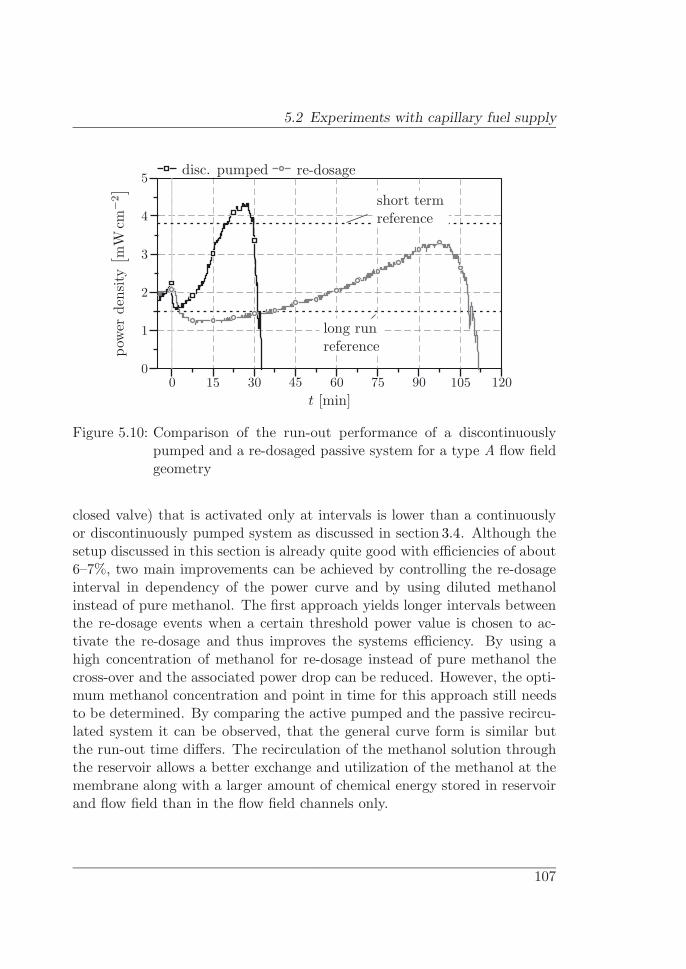
5.2 Experiments with capillary fuel supply
disc. pumped re-dosage
pow
erde
nsity
[ mW
cm−2
]
t [min]
long runreference
short termreference
0
1
2
3
4
5
0 15 30 45 60 75 90 105 120
Figure 5.10: Comparison of the run-out performance of a discontinuouslypumped and a re-dosaged passive system for a type A flow fieldgeometry
closed valve) that is activated only at intervals is lower than a continuouslyor discontinuously pumped system as discussed in section 3.4. Although thesetup discussed in this section is already quite good with efficiencies of about6–7%, two main improvements can be achieved by controlling the re-dosageinterval in dependency of the power curve and by using diluted methanolinstead of pure methanol. The first approach yields longer intervals betweenthe re-dosage events when a certain threshold power value is chosen to ac-tivate the re-dosage and thus improves the systems efficiency. By using ahigh concentration of methanol for re-dosage instead of pure methanol thecross-over and the associated power drop can be reduced. However, the opti-mum methanol concentration and point in time for this approach still needsto be determined. By comparing the active pumped and the passive recircu-lated system it can be observed, that the general curve form is similar butthe run-out time differs. The recirculation of the methanol solution throughthe reservoir allows a better exchange and utilization of the methanol at themembrane along with a larger amount of chemical energy stored in reservoirand flow field than in the flow field channels only.
107


6 Summary and outlook
During the previous chapters active and passive fuel cell systems have beenstudied with focus on the anode side flow field. In a first step, a referencecell has been studied and an approach how this continuously pumped systemcan be improved by changing to an operation with pumping at intervals.The results showed that an improvement of the mean power performance by1.7–2.9× compared to the reference measurements is possible. This denotesthat a performance improvement can be achieved for most persisting activeDMFC systems by using a discontinuous pumping method while deliveringthe equivalent amount of methanol. CFD-simulations have been used toverify that the channel design of the flow fields can be used to pump thefuel by using the movement of the developing carbon dioxide gas bubbles.The simulation results were compared to experiments with single flow fieldchannel and artificial bubble generation, using syringe pumps. Though thesimulations proofed qualitatively that fuel recirculation is feasible, the flowrates measured in the experiments for the A and B-type channels are muchlower. But also these experiments do not reflect the real fuel cell properly asthe flow rates for the B-type channels are even below the minimum requiredmethanol flow rate. By measuring the flow rate during fuel cell operation theminimum required flow rate for long term fuel cell operation of 1.55µL min−1
at a load of 20mAcm−2 is exceeded by 5–16× for all channel types, includingthe R-type channel. Therefore a stable long term operation of the fuel cellis possible. In the experiments with the passive fuel cell setup it has beenshown that the achieved mean power density of each flow field type is higherthan the reference power density achieved in the active fuel cell setup. Thisis valid for both studied fuel supply methods: supplying a certain volumeof methanol solution and re-dosage of methanol at intervals. By increasingthe volume of the supplied 4M methanol solution from 2.0mL to 9.1mL, anoperation of over 15 hours for each of the flow field channel types in a passive
109
6 Summary and outlook
setup has been achieved. The efficiency η has been about 10% in these longterm experiments and the run time was limited by the amount of providedfuel.
The following paragraphs give an outlook for future work based on the resultspresented in this thesis. Starting with the active, continuous pumped systemstudied in Chapter 3, the next step is to identify a pump with low energydemand and overall size that is able to deliver a flow rate of 4mL h−1. Theapproach to pump at intervals showed that an improvement of the meanpower density of the reference Pref = 1.6mWcm−2 to 2.5–4.3mWcm−2 ispossible. It is expected that changing from a regular pumping interval to aperformance driven approach will yield a further performance improvementdue to the following reasons: First, the pump is only activated when fresh fuelis required and therefore energy for peripherals can be reduced. Second, ahigh fuel utilization is achieved due to long fuel residence time in the flow field.Third, reducing the amount of methanol solution that is pumped through thesystem to the volume of the flow field and the supply channels reduces theenergy required for the pump and waste amount.
The simulation models used in Chapter 4 show that bubble dynamics intapered structures can be modelled with a deviation of about 20% for thegas bubble movement. The model with the flow field channel and the reservoirgives qualitative correct results but overestimates the generated liquid flowrate when compared to the single channel experiments. Nevertheless it allowsto study the different pumping mechanisms and the effects of the differentbubble shapes on the liquid flow. By relocating the gas injection points in thesingle channel experiments to the sides of the channels, especially the B-typechannel, should result in a better agreement with the flow rates measured inthe fuel cell, since gas bubbles block parts of the side channels and increasethe fluidic resistance inside the channel resulting in a higher outer flow rate.
Regarding the passive system experiments in chapter 5, it has been shownthat although the flow rates differ for the three channel types, the long termperformance is almost identical, as long as there is a virtual check valve inthe R-type channel. This yields that the flow rate does not influence thepower performance of the fuel cell. Except of further increasing the reservoirsize there is no immediate possibility to improve the performance of the fuel
110

cell as studied here. For a new setup with type A or B channels, downscalingof the flowfield channels to reduce effects due to gravity might be consid-ered. This will allow a fuel cell setup that is independent of its operation asalready proposed in [114]. But as discussed in section 2.4, the channel sizestill has to provide enough space for fluid flow when the membrane is wettedand swollen. First experiments showing this improved and downscaled flowfield are shown in [118]. The approach of re-dosing methanol into the reser-voir with a methanol solution has been studied. This setup showed a lowerefficiency than the results achieved with the fully passive setup and for thesystem design an active re-dosage unit like a pump is required. Neverthelessthere is the potential to improve this setup significantly and it will probablybe even better than the passive system: First, like in the setup with pump-ing at intervals, the re-dosage could be triggered by a threshold value of thepower output instead of regular intervals resulting in less re-dosage events.Second, in order to avoid too high water loss and increase of methanol con-centration at the anode, a methanol solution with high concentration insteadof pure methanol should be used. Third, when targeting at longer run-timesthis method becomes more attractive since the energy density of the sys-tem is significantly increased compared to a large reservoir with a pre-mixedmethanol solution and comparably low methanol concentration.
Some of the observations made during the different experiments in this workare relevant for the cathode design or the overall system design. During theexperiments water droplet formation has been observed at the cathode sideof the fuel cell, blocking parts of the active area there. To better control thewater droplets and remove them from the cathode active area an adaptedapproach for water removal could be used based on the results from Metzet al [119–121] who used it for a hydrogen fuel cell. The cathode designthen comprises a non-clogging flow field that supports passive water removaland still allows for diffusive oxygen supply. Another possibility to achievethe same result is the use of a microstructured hydrophilic porous carbonmaterial as proposed by Paust et al [118]. In this approach, a liquid waterdroplet is sucked into the porous material as soon as it gets into contact withthe flow field and is then passively transported away from the membranedue to capillarity. The combination of an improved, downscaled anode anda water removing cathode will increase the fuel cell power performance.
111

6 Summary and outlook
6.1 Design guidelines
For the improvement of the overall system and its energy density a hybrid,semi-passive system with a tapered channel design and re-dosage of methanolinto the reservoir is the best approach because:
� As shown in the previous chapter, a passive system yields a betterperformance than the active reference system and enables a long termstable operation with passive fuel recirculation.
� A tapered channel design yields a predetermined flow direction whilein a straight channel design the flow direction can differ in each of theflow field channels.
� Re-dosage of pure methanol or a solution with high methanol concen-tration increases the overall energy density of the system although theperformance shown in the previous chapter is below the completelypassive system.
� The fuel cell can be run under optimum performance condition whilethe secondary battery is used to drive the load and the re-dosage unit,e.g. a micropump
� A performance dependent re-dosage interval keeps the energy demandof the peripherals low.
Some of the topics addressed above are covered in the enhanced fuel cellsystem developed by Nils Paust at the Laboratory of MEMS Applications,University of Freiburg, Germany.
112
Bibliography
[1] M. Winter and R. J. Brodd. What are batteries, fuel cells, and super-capacitors? Chemical Reviews, 104(10):4245–4269, 2004.
[2] C. K. Dyer. Fuel cells for portable applications. Journal of PowerSources, 106(1-2):31–34, 2002.
[3] Fuel Cell Today. www.fuelcelltoday.com, 2006.
[4] M. Cropper. Fuel cell market survey: Portable applications. Report,2002.
[5] M. Cropper. Fuel cell market survey: Portable applications. Report,2003.
[6] D. Jollie. Fuel cell market survey: Portable applications. Report, 2004.
[7] A. Baker, D. Jollie, and K.-A. Adamson. Fuel Cell Today market sur-vey: Portable applications. Report, 2005.
[8] D. Ilic, K. Holl, P. Birke, T. Wohrle, F. Birke-Salam, A. Perner, andP. Haug. Fuel cells and batteries: Competition or separate paths?Journal of Power Sources, 155(1):72–76, 2006.
[9] H. Dohle, J. Divisek, and R. Jung. Process engineering of the directmethanol fuel cell. Journal of Power Sources, 86(1-2):469–477, 2000.
[10] A. S. Arico, S. Srinivasan, and V. Antonucci. DMFCs: From funda-mental aspects to technology development. Fuel Cells, 1(2):133–161,2001.
[11] X. Ren, P. Zelenay, S. Thomas, J. Davey, and S. Gottesfeld. Recent ad-vances in direct methanol fuel cells at Los Alamos National Laboratory.Journal of Power Sources, 86(1-2):111–116, 2000.
113

Bibliography
[12] S. Cleghorn, X. Ren, S. Thomas, and S. Gottesfeld. In Book of ExtendedAbstracts, pages 218–219. ISE-ECS Joint Symposium, 1997.
[13] W. M. Qian, D. P. Wilkinson, J. Shen, H. J. Wang, and J. J. Zhang.Architecture for portable direct liquid fuel cells. Journal of PowerSources, 154(1):202–213, 2006.
[14] E. Sakaue. Micromachining / Nanotechnology in direct methanol fuelcell. In IEEE MEMS 2005, pages 600–605. 2005.
[15] G. McLean. Fuel cell architectures for portable power applications. InSmall Fuel Cells 2005, The Knowledge Foundations Seventh AnnualInternational Symposium. 27–29.4.2005.
[16] Toshiba announces world’s smallest direct methanol fuel cell with en-ergy output of 100 milliwatts. Toshiba: Press Releases, 24.6.2004.http://www.toshiba.co.jp/about/press/2004 06/pr2401.htm.
[17] C. Litterst, S. Eccarius, C. Hebling, R. Zengerle, and P. Koltay. In-creasing µDMFC efficiency by passive CO2 bubble removal and discon-tinuous operation. Journal of Micromechanics and Microengineering,16(9):S248–S253, 2006.
[18] A. K. Shukla, P. A. Christensen, A. Hamnett, and M. P. Hogarth. Avapor-feed direct-methanol fuel-cell with proton-exchange membraneelectrolyte. Journal of Power Sources, 55(1):87–91, 1995.
[19] J. Kallo, W. Lehnert, and R. von Helmolt. Conductance and methanolcrossover investigation of Nafion membranes in a vapor-fed DMFC. J.Electrochem. Soc., 150(6):A765–A769, 2003.
[20] J. Kallo, J. Kamara, W. Lehnert, and R. von Helmolt. Cell voltagetransients of a gas-fed direct methanol fuel cell. Journal of PowerSources, 127(1-2):181–186, 2004.
[21] Z. H. Jiang and R. A. Dougal. Real-time strategy for active power shar-ing in a fuel cell powered battery charger. Journal of Power Sources,142(1-2):253–263, 2005.
114

Bibliography
[22] N. T. Nguyen and S. H. Chan. Micromachined polymer electrolytemembrane and direct methanol fuel cells - a review. Journal of Mi-cromechanics and Microengineering, 16(4):R1–R12, 2006.
[23] R. Hahn, S. Wagner, A. Schmitz, and H. Reichl. Development of aplanar micro fuel cell with thin film and micro patterning technologies.Journal of Power Sources, 131(1-2):73–78, 2004.
[24] D. Modroukas, V. Modi, and L. G. Frechette. Micromachined siliconstructures for free-convection PEM fuel cells. J. Micromech. Microeng.,15(9):S193–S201, 2005.
[25] A. Kumar and R. G. Reddy. Materials and design development forbipolar�end plates in fuel cells. Journal of Power Sources, 129(1):62–67, 2004.
[26] T. Shimizu, T. Momma, M. Mohamedi, T. Osaka, and S. Sarangapani.Design and fabrication of pumpless small direct methanol fuel cells forportable applications. Journal of Power Sources, 137(2):277–283, 2004.
[27] D. J. Kim, E. A. Cho, S. A. Hong, I. H. Oh, and H. Y. Ha. Recentprogress in passive direct methanol fuel cells at KIST. Journal of PowerSources, 130(1-2):172–177, 2004.
[28] J. G. Liu, T. S. Zhao, R. Chen, and C. W. Wong. The effect of methanolconcentration on the performance of a passive DMFC. ElectrochemistryCommunications, 7(3):288–294, 2005.
[29] S. W. Cha, R. O’Hayre, and F. B. Prinz. The influence of size scaleon the performance of fuel cells. Solid State Ionics, 175(1-4):789–795,2004.
[30] K. Wozniak, D. Johansson, M. Bring, A. Sanz-Velasco, and P. Enoks-son. A micro direct methanol fuel cell demonstrator. Journal of Mi-cromechanics and Microengineering, 14(9):S59–S63, 2004.
[31] M. Muller, C. Muller, F. Gromball, M. Wolfle, and W. Menz. Micro-structured flow fields for small fuel cells. Microsyst. Technol., 9(3):159–162, 2003.
115

Bibliography
[32] M. A. Muller, C. Muller, R. Forster, and W. Menz. Carbon paperflow fields made by WEDM for small fuel cells. Microsyst. Technol.,11(4):280–281, 2005.
[33] S. W. Cha, R. O’Hayre, Y. Saito, and F. B. Prinz. The scaling behaviorof flow patterns: a model investigation. Journal of Power Sources,134(1):57–71, 2004.
[34] T. J. Yen, N. Fang, X. Zhang, G. Q. Lu, and C. Y. Wang. A micromethanol fuel cell operating at near room temperature. Applied PhysicsLetters, 83(19):4056–4058, 2003.
[35] S. S. Hsieh, J. K. Kuo, C. F. Hwang, and H. H. Tsai. A novel designand microfabrication for a micro PEMFC. Microsystem Technologies-Micro-and Nanosystems-Information Storage and Processing Systems,10(2):121–126, 2004.
[36] S. H. Chan, N. T. Nguyen, Z. T. Xia, and Z. G. Wu. Development of apolymeric micro fuel cell containing laser-micromachined flow channels.Journal of Micromechanics and Microengineering, 15(1):231–236, 2005.
[37] C. Xie, J. Bostaph, and J. Pavio. Development of a 2W direct methanolfuel cell power source. J. Power Sources, 136(1):55–65, 2004.
[38] K. Tuber, A Oedegaard, M. Herrmann, and C. Hebling. Investigationof fractal flow-fields in portable proton exchange membrane and directmethanol fuel cells. J. Power Sources, 131(1-2):175–181, 2004.
[39] H. Dohle, T. Bewer, J. Mergel, R. Neitzel, and D. Stolten. Evaluationof flow field designs for use in PEM and DMFC fuel cells. In Abstractsof the 2000 Fuel Cell Seminar, pages 130–133. 2000.
[40] S. Q. Song, Z. X. Liang, W. J. Zhou, G. Q. Sun, Q. Xin, V. Ster-giopoulos, and P. Tsiakaras. Direct methanol fuel cells: The effect ofelectrode fabrication procedure on meas structural properties and cellperformance. J. Power Sources, 145(2):495–501, 2005.
[41] J. G. Liu, T. S. Zhao, Z. X. Liang, and R. Chen. Effect of membranethickness on the performance and efficiency of passive direct methanolfuel cells. J. Power Sources, 153(1):61–67, 2006.
116

Bibliography
[42] H. Yang and T. S. Zhao. Effect of anode flow field design on theperformance of liquid feed direct methanol fuel cells. ElectrochimicaActa, 50(16-17):3243–3252, 2005.
[43] H. Yang, T. S. Zhao, and Q. Ye. Pressure drop behavior in the anodeflow field of liquid feed direct methanol fuel cells. Journal of PowerSources, 142(1-2):117–124, 2005.
[44] A Oedegaard, S. Hufschmidt, R. Wilmshoefer, and C. Hebling. PortableSize DMFC-Stack. Fuel Cells, 4(3):219–224, 2004.
[45] A. S. Arico, P. Creti, V. Baglio, E. Modica, and V. Antonucci. Influenceof flow field design on the performance of a direct methanol fuel cell.J. Power Sources, 91(2):202–209, 2008.
[46] ROBERT BOSCH GMBH, M. Ruoff, M. Nau, M. Bareis, H. Harn-dorf, and F. Ilgner. (EN) Device for supplying the consumers of a fuelcell system with liquid media; (DE) Vorrichtung zur Zufuhr flussigerMedien zu Verbrauchern einer Brennstoffzellenanlage. Patent, Sep2001. Pub. No.: WO/2001/024294; International Application No.:PCT/DE2000/003340.
[47] R. Zengerle, M. Leitner, S. Kluge, and A. Richter. Carbon dioxidepriming of micro liquid systems. In Proceedings of IEEE-MEMS 1995,pages 340–343. 1995.
[48] Z. Guo and Y. Cao. A passive fuel delivery system for portable directmethanol fuel cells. Journal of Power Sources, 132(1-2):86–91, 2004.
[49] Q. Ye and T. S. Zhao. A natural-circulation fuel delivery system fordirect methanol fuel cells. Journal of Power Sources, 147(1-2):196–202,2005.
[50] J. Zhang, K. Colbow, A. Lee, and B. Lin. Reactant feed apparatus fordirect feed fuel cells and methods related thereto. Patent, Jan 2004.
[51] D-S. Meng, T. Cubaud, C-M Ho, and C. J. Kim. A membrane breatherfor micro fuel cells with high concentration methanol. In Hilton Head2004: A Solid State Sensor, Actuator and Microsystems Workshop.2004.
117

Bibliography
[52] D. D. S. Meng, J. Kim, and C. J. Kim. A degassing plate with hy-drophobic bubble capture and distributed venting for microfluidic de-vices. Journal of Micromechanics and Microengineering, 16(2):419–424,2006.
[53] D. D. Meng and C.-J. Kim. Embedded self-circulation of liquid fuel fora micro direct methanol fuel cell. In Proceedings of IEEE MEMS 2007,pages 85–88. 2007.
[54] J. Kohnle, G. Waibel, R. Cernosa, M. Storz, H. Ernst, H. Sandmaier,T. Strobelt, and R. Zengerle. A unique solution for preventing cloggingof flow channels by gas bubbles. In IEEE MEMS, pages 77–80. The 15thinternational ieee micro electro mechanical conference edition, 2002.
[55] G. Waibel, J. Kohnle, R. Cernosa, M. Storz, M. Schmitt, H. Ernst,H. Sandmaier, R. Zengerle, and T. Strobelt. Highly integrated au-tonomous microdosage system. Sensors and Actuators A-Physical,103(1-2):225–230, 2003.
[56] C. Litterst, J. Kohnle, H. Ernst, S Messner, H. Sandmaier, R. Zengerle,and P. Koltay. Improved gas bubble mobility in CHIC-type flow chan-nels. In Hubert Borgmann, editor, ACTUATOR, pages 541–544. 2004.
[57] C. Litterst, T. Metz, R. Zengerle, and P. Koltay. Static and dynamicbehaviour of gas bubbles in T-shaped non-clogging micro-channels. Mi-crofluidics and Nanofluidics, 5(6):775–784, 2008. DOI 10.1007/s10404-008-0279-3.
[58] P. Koltay, C. Litterst, and S. Eccarius. (EN) Device compris-ing a channel carrying a medium and method for removing inclu-sions; (DE) Vorrichtung mit einem ein Medium fuhrenden Kanalund Verfahren zur Entfernung von Einschlussen. Patent, Jan2006. Pub. No.: WO/2006/082087; International Application No.:PCT/EP2006/000990.
[59] C. Litterst, S. Eccarius, C. Hebling, R. Zengerle, and P. Koltay. Novelstructure for passive CO2 degassing in µDMFC. In Proceedings of Pow-erMEMS 2005, pages 194–197. 2005.
118

Bibliography
[60] C. L. Yaws. Handbook of Transport Property Data: Viscosity, ThermalConductivity, and Diffusion Coefficients of Liquids and Gases (Libraryof Physico-Chemical Property Data). Gulf Pub Co, Houston, TX, 1995.
[61] Y. Daiko, L. C. Klein, and M. Nogami. Modifying Nafion with nanos-tructured inorganic oxides for proton exchange membrane fuel cells. InE. M. Kelder, E. R. Leite, J.-M. Tarascon, and Y.-M. Chiang, editors,Nanostructured Materials in Alternative Energy Devices, volume 822of Proceedings of Materials Research Society Symposium, pages S8.4.1–S8.4.6. 2004.
[62] FWB - Kunststofftechnik GmbH. Blocksberg 175, D-66955 Pirmasens,Germany, 2006. http://www.fwb-gmbh.de.
[63] Fraunhofer Institute for Solar Energy Systems (ISE). Heidenhofstr. 2,D-79110 Freiburg, Germany, 2006. www.ise.fraunhofer.de.
[64] Dr. Collin GmbH. Sportparkstr. 2, D-85560 Ebersberg, Germany,11.07.2006. http://www.drcollin.de.
[65] SolviCore GmbH & Co. KG. Rodenbacher Chaussee 4, 63457 Hanau-Wolfgang, Germany, 2007. http://www.solvicore.umicore.com.
[66] SGL CARBON AG. Rheingaustr. 182–184, 65203 Wiesbaden, Ger-many, 2004. http://www.sglgroup.com.
[67] Elastosil� RT 607. Wacker Chemie AG, http://www.wacker.com,2007.
[68] Silicone rubber compound - flowable liquid, RS 692-542. RS Compo-nents GmbH, http://www.rsonline.de, 2002.
[69] P. Argyropoulos, K. Scott, and W. M. Taama. Carbon dioxide evolutionpatterns in direct methanol fuel cells. Electrochimica Acta, 44(20):3575–3584, 1999.
[70] G. Q. Lu and C. Y. Wang. Electrochemical and flow characterizationof a direct methanol fuel cell. Journal of Power Sources, 134(1):33–40,2004.
119
Bibliography
[71] H. Yang, T. S. Zhao, and Q. Ye. In situ visualization study of CO2 gasbubble behavior in DMFC anode flow fields. Journal of Power Sources,139(1-2):79–90, 2005.
[72] C. W. Wong, T. S. Zhao, Q. Ye, and J. G. Liu. Transient capillaryblocking in the flow field of a micro-DMFC and its effect on cell per-formance 1. J. Electrochem. Soc., 152(8):A1600–A1605, 2005.
[73] T. Bewer, T. Beckmann, H. Dohle, J. Mergel, and D. Stolten. Novelmethod for investigation of two-phase flow in liquid feed direct methanolfuel cells using an aqueous H2O2 solution. Journal of Power Sources,125(1):1–9, 2004.
[74] N. Paust, C. Litterst, T. Metz, R. Zengerle, and P. Koltay. Gasblasen-getriebene Pumpe fur Mikroreaktoren. In VDI-VDE-IT, editor, Pro-ceedings of MikroSystemTechnik Kongress, pages 481–484. VDE Verlag,Oct 2007.
[75] N. Paust, C. Litterst, T. Metz, M. Eck, R. Zengerle, and P. Koltay.Capillary driven fuel supply in direct methanol fuel cells with doubletapered T-shaped channel flow fields. In Proceedings of PowerMEMS2007, pages 185–188. 2007.
[76] N. Paust, C. Litterst, T. Metz, R. Zengerle, and P. Koltay. Fully passivedegassing and fuel supply in direct methanol fuel cells. In Proceedings ofthe 21st IEEE International Conference on Micro Electro MechanicalSystems, MEMS, pages 34–37. 2008.
[77] TTi - Thurlby Thandar Instruments. 2007.
[78] B. Braun Melsungen AG. Carl-Braun-Straße, 134212 Melsungen, Ger-many, 2008. http://www.bbraun.de.
[79] CFD-ACE+, ESI CFD, Inc., Huntsville, AL., 2006. Version 2006.0.14,http://www.cfdrc.com.
[80] J. D. Anderson. Computational Fluid Dynamics. McGraw-Hill Sci-ence/Engineering/Math, 1 edition, 1995.
120

Bibliography
[81] J. P. Vandoormaal and G. D. Raithby. Enhancements of the sim-ple method for predicting incompressible fluid-flows. Numerical HeatTransfer, 7(2):147–163, 1984.
[82] C. W. Hirt, B. D. Nichols, and N. C. Romero. SOLA - A numeri-cal solution algorithm for transient fluid flows. Los Alamos NationalLaboratory Report, LA-5852, 1975.
[83] B. D. Nichols, C. W. Hirt, and R. S. Hotchkiss. SOLA-VOF: A solutionalgorithm for transient fluid flow with multiple free boundaries. LosAlamos National Laboratory Report, LA-8355, 1980.
[84] M. R. Barkhudarov and S. B. Chin. Stability of a numerical algorithmfor gas bubble modeling. International Journal for Numerical Methodsin Fluids, 19(5):415–437, 1994.
[85] M. R. Barkhudarov. Semi-Lagrangian VOF advection method forFLOW-3D. Flow Science Technical Note, (FSI-03-TN63), 2003.
[86] C. W. Hirt and B. D. Nichols. Volume of fluid (VOF) method forthe dynamics of free boundaries. Journal of Computational Physics,39(1):201–225, 1981.
[87] W. J. Rider, D. B. Kothe, S. J. Mosso, J. H. Cerutti, and J. I. Hochstein.Accurate solution algorithms for incompressible multiphase flows. Re-port, 1994.
[88] D. B. Kothe and W. J. Rider. Comments on modeling interfacial flowswith Volume-of-Fluid methods. Report, 1995.
[89] J. E. Pilliod and E. G. Puckett. Second-order accurate volume-of-fluidalgorithms for tracking material interfaces. Journal of ComputationalPhysics, 199(2):465–502, 2004.
[90] D. Lorstad and L. Fuchs. High-order surface tension VOF-model for3D bubble flows with high density ratio. Journal of ComputationalPhysics, 200(1):153–176, 2004.
[91] M. V. Annaland, N. G. Deen, and J. A. M. Kuipers. Numerical sim-ulation of gas bubbles behaviour using a three-dimensional volume offluid method. Chemical Engineering Science, 60(11):2999–3011, 2005.
121

Bibliography
[92] J. Eggers. Theory of drop formation. Physics of Fluids, 7(5):941–953,1995.
[93] H. K. Versteeg and M. Malalasekera. An Introduction to ComputationalFluid Dynamics. The Finite Volume Method. Prentice Hall, 1996.
[94] S. Anghaie and G. Chen. Adoption of single-phase CFD to two-phaseflow and heat transfer problems. In Proceedings of Workshop on Com-puting Methods for Two-Phase Flow, 2000.
[95] S. J. Cummins, M. M. Francois, and D. B. Kothe. Estimating curvaturefrom volume fractions. Computers & Structures, 83(6-7):425–434, 2005.
[96] J. U. Brackbill, D. B. Kothe, and C. Zemach. A continuum methodfor modeling surface-tension. Journal of Computational Physics,100(2):335–354, 1992.
[97] P. Sonneveld. CGS, a fast Lanczos-type solver for nonsymmetriclinear-systems. Siam Journal on Scientific and Statistical Computing,10(1):36–52, 1989.
[98] U. Trottenberg, C. W. Oosterlee, and A. Schuller. Multigrid. AcademicPress, 2001.
[99] Z. H. Wang and C. Y. Wang. Mathematical modeling of liquid-feeddirect methanol fuel cells. J. Electrochem. Soc., 150(4):A508–A519,2003.
[100] X. Li, E. P. L. Roberts, and S. M. Holmes. Evaluation of compositemembranes for direct methanol fuel cells. J. Power Sources, 154(1):115–123, 2006.
[101] K. W. Lum and J. J. McGuirk. Three-dimensional model of a completepolymer electrolyte membrane fuel cell - model formulation, validationand parametric studies. J. Power Sources, 143(1-2):103–124, 2005.
[102] J. P. Meyers and J. Newman. Simulation of the direct methanol fuel cell- ii. modeling and data analysis of transport and kinetic phenomena.J. Electrochem. Soc., 149(6):A718–A728, 2002.
122
Bibliography
[103] J. Divisek, J. Fuhrmann, K. Gartner, and R. Jung. Performance mod-eling of a direct methanol fuel cell. J. Electrochem. Soc., 150(6):A811–A825, 2003.
[104] T. Metz and N. Paust. Experiments and simulation of gas bubblesmoving in tapered channels. Personal communication, Laboratory forMEMS applications, University of Freiburg, Germany, 2007.
[105] H. L. Wang and Y. Wang. Flow in microchannels with rough walls:flow pattern and pressure drop. Journal of Micromechanics and Micro-engineering, 17(3):586–596, 2007.
[106] A. S. Rawool, S. K. Mitra, and S. G. Kandlikar. Numerical simulationof flow through microchannels with designed roughness. Microfluidicsand Nanofluidics, 2(3):215–221, 2006.
[107] M. J. de Ruijter, T. D. Blake, and J. De Coninck. Dynamic wettingstudied by molecular modeling simulations of droplet spreading. Lang-muir, 15(22):7836–7847, 1999.
[108] T. Glatzel, C. Cupelli, T. Lindemann, C. Litterst, Ch. Moosmann,R. Niekrawietz, W. Streule, R. Zengerle, and P. Koltay. Computationalfluid dynamics (CFD) software tools for microfluidic applications - Acase study. Computers & Fluids, 37(3):218–235, 2008.
[109] E. W. Lemmon, M. O. MacLinden, and D. G. Friend. Thermophysicalproperties of fluid systems. In P. J. Linstrom and W. G. Mallard,editors, NIST Chemistry WebBook, NIST Standard Reference DatabaseNumber 69. National Institute of Standards and Technology, 2005.
[110] N. Paust, 2007. Personal communication, Laboratory for MEMS ap-plications, University of Freiburg, Germany.
[111] J. H. Ferziger and M. Peric. Computational Methods for Fluid Dynam-ics. Springer, 3rd rev. ed. edition, 2002.
[112] Sensirion AG - ASL1430. http://www.sensirion.com, 2006.
[113] Polytec PT GmbH. Polymere Technologien, Polytec-Platz 1-7, D-76337Waldbronn, Germany, 2008. http://www.polytec-pt.com.
123

Bibliography
[114] N. Paust, C. Litterst, T. Metz, M. Eck, C Ziegler, R. Zengerle, andP. Koltay. Capillary-driven pumping for passive degassing and fuelsupply in direct methanol fuel cells. Microfluidics and Nanofluidics,2009. published online Feb. 20, 2009.
[115] X. Ren, T. E. Springer, and S. Gottesfeld. In S. Gottesfeld and T. F.Fuller, editors, Proton Conducting Membrane Fuel Cells – Second In-ternational Symposium, volume 98-27, pages 341–357. ElectrochemicalSociety, 1999.
[116] Alcan Inc. 1188 Sherbrooke Street West, Montreal, Quebec H3A 3G2,Canada, 2009. www.alcan.com.
[117] J. Ducree, S. Haeberle, S. Lutz, S. Pausch, F. von Stetten, andR. Zengerle. The centrifugal microfluidic Bio-Disk platform. J. Mi-cromech. Microeng., 17:S103–S115, 2007.
[118] N. Paust, S. Krumbholz, S. Munt, C. Muller, R. Zengerle, C Ziegler,and P. Koltay. Design of a passive and portable DMFC operating in allorientations. In Proceedings of IEEE MEMS 2009, pages 1091–1094.2009.
[119] T. Metz, N. Paust, C. Muller, R. Zengerle, and P. Koltay. Micro struc-tured flow field for passive water management in miniaturized PEMfuel cells. In Proceedings of the 20th IEEE International Conference onMicro Electro Mechanical Systems, MEMS, 2007.
[120] T. Metz, N. Paust, C. Muller, R. Zengerle, and P. Koltay. Passivewater removal in fuel cells by capillary droplet actuation. Sensors &Actuators: A. Physical, Special Issue MEMS 2007, 2007.
[121] T. Metz, S. Kerzenmacher, N. Paust, C. Muller, R. Zengerle, andP. Koltay. Passive water management system for pem fuelcells usingmicrostructures. In Proceedings of PowerMEMS 2007, pages 177–180.2007.
124

Annex A
Glossary
Parameter Description
A AreaCx Concentration of the substance xCa Capillary numberD Diffusion constantEel Electrical energyF Scalar field variable in VOF simulations;
Specifies the fraction of the volume of eachcomputational cell in the grid occupied bythe second fluid
I Electrical currentj Current densityNA Avogadro constant; NA = 6.02214 1023 mol−1
P PowerPcap Capillary pressurePref,lrr Long run reference power densityPref,str Short term reference power densityR ResistorT TemperatureU VoltageVm Molar Volume
Continued on next page
125

Annex A Glossary
Parameter Description
Wc Chemical energy∆C Concentration differenceΦ Methanol consumption in diffusion
model (c.f. section 2.4)Θ Contact angleη Efficiencyλ Solubility coefficient for a gas in
a water solutionφ Liquid flow rateπ 3.142ρ Densitya cross-sectional area; source area in diffusion
model (c.f. section 2.4)d Diameter or distance between two pointse Elementary charge; e = 1.6021892 10−19 As
j Current densitymm Molar massne Number of available electrons per methanol
moleculer Radius or curvature radiust Time�v Velocity vector
126
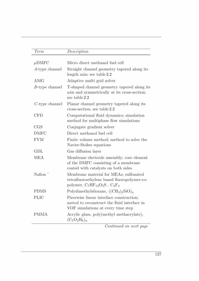
Term Description
µDMFC Micro direct methanol fuel cellA-type channel Straight channel geometry tapered along its
length axis; see table 2.2AMG Adaptive multi grid solverB-type channel T-shaped channel geometry tapered along its
axis and symmetrically at its cross-section;see table 2.2
C -type channel Planar channel geometry tapered along itscross-section; see table 2.2
CFD Computational fluid dynamics; simulationmethod for multiphase flow simulations
CGS Conjugate gradient solverDMFC Direct methanol fuel cellFVM Finite volume method; method to solve the
Navier-Stokes equationsGDL Gas diffusion layerMEA Membrane electrode assembly; core element
of the DMFC consisting of a membranecoated with catalysts on both sides
Nafion� Membrane material for MEAs; sulfonatedtetrafluoroethylene based fluoropolymer-co-polymer, C7HF13O5S . C2F4
PDMS Polydimethylsiloxane, ((CH3)2SiO)nPLIC Piecewise linear interface construction;
metod to reconstruct the fluid interface inVOF simulations at every time step
PMMA Acrylic glass, poly(methyl methacrylate),(C5O2H8)n
Continued on next page
127

Annex A Glossary
Term Description
R-type channel Reference geometry as a straight channelwithout any tapering angles; see table 2.2
rds Rate determining step; step in a chemicalreaction that delimits the overall reactionspeed
VOF Volume of fluid; method to model freesurface flows in CFD-simulations
128

Annex B
Design parameters and dimensions
Table B.1: Design parameters and dimensions of the different channels R, A,B and C described in the thesis
Type Sketch Dimension
R
h
wl
h = 1.0mmw = 3.0mml = 20.0mm
Aα
h
wl
h = 0.8mmw = 3.0mml = 20.0mmα = 1.5 � or 3.0 �
B α
β
h wl
H
Wh = 0.3mmH = 0.8mmw = 3.0mmW= 0.8mml = 20mmα = 1.5 � or 3.0 �β = 7.0 �
C α
h
wl
h = 0.2mmw = 1.49mm or 1.17mml = 20mmα = 1.5 � or 3.0 �
129

Annex B Design parameters and dimensions
AA
4.0
65.0
4.0
M3
43.0
A–A
M6
6.0
13.013.013.03.03.0
10.0
2.02.
02.
024
.0
1.0
3�
Figure B.1: Dimensions of the moulding tool used for the hot embossing.For the detailed dimensions of the evenly spaced channels seetableB.1
130

A A
A–A
5.0
�3.5×2
2.0
2.0
2.0
2.020.0
4.0
4.0�3.4
�1.5
3.0
43.0
10.0
13.0
65.0
Figure B.2: Dimensions of the test samples for activesystem setups. This samples are connectedthrough the drilled wholes shown in the sec-tional view A–A. For the detailed dimensionsof the evenly spaced channels see tableB.1
131

Annex B Design parameters and dimensions
A A
A–A
5.0
10�
2.0
2.0
2.020.0
4.0
4.0�3.4
3.0
43.0
10.0
13.0
65.0
Figure B.3: Dimensions of the test samples for passivesystem setups. The fuel cells are suppliedthrough the slotted wholes as depicted inthe sectional view A–A. For the detailed di-mensions of the evenly spaced channels seetableB.1
132

Annex C
Picture sequences
The picture sequences on the following pages show:
� FigureC.1: Bubble development in a passive type R flow field over 60 sat a load of I = 60mA with a 4M methanol solution
� FigureC.2: Bubble development in a passive type A flow field over 60 sat a load of I = 60mA with a 4M methanol solution
� FigureC.3: Bubble development in a passive type B flow field over 60 sat a load of I = 60mA with a 4M methanol solution
� FigureC.4: Comparison of a single type R, A and B-channel in a pas-sively operated fuel cell at a load of I = 60mA with a 4M methanolsolution over a period of 60 s.
133

Annex C Picture sequences
t = 0 s
t = 2 s
t = 4 s
t = 6 s
t = 8 s
t = 10 s
t = 12 s
t = 14 s
t = 16 s
t = 18 s
t = 20 s
t = 22 s
t = 24 s
t = 26 s
t = 28 s
t = 30 s
t = 32 s
t = 34 s
t = 36 s
t = 38 s
t = 40 s
t = 42 s
t = 44 s
t = 46 s
t = 48 s
t = 50 s
t = 52 s
t = 54 s
t = 56 s
t = 58 s
Figure C.1: Bubble development in a type R channel over a period of t = 60 sat a load of I = 60mA with a 4M methanol solution
134

FD t = 0 s
t = 2 s
t = 4 s
t = 6 s
t = 8 s
t = 10 s
t = 12 s
t = 14 s
t = 16 s
t = 18 s
t = 20 s
t = 22 s
t = 24 s
t = 26 s
t = 28 s
t = 30 s
t = 32 s
t = 34 s
t = 36 s
t = 38 s
t = 40 s
t = 42 s
t = 44 s
t = 46 s
t = 48 s
t = 50 s
t = 52 s
t = 54 s
t = 56 s
t = 58 s
Figure C.2: Bubble development in a type A channel over a period of t = 60 sat a load of I = 60mA with a 4M methanol solution
135

Annex C Picture sequences
FD t = 0 s
t = 2 s
t = 4 s
t = 6 s
t = 8 s
t = 10 s
t = 12 s
t = 14 s
t = 16 s
t = 18 s
t = 20 s
t = 22 s
t = 24 s
t = 26 s
t = 28 s
t = 30 s
t = 32 s
t = 34 s
t = 36 s
t = 38 s
t = 40 s
t = 42 s
t = 44 s
t = 46 s
t = 48 s
t = 50 s
t = 52 s
t = 54 s
t = 56 s
t = 58 s
Figure C.3: Bubble development in a type B channel over a period of t = 60 sat a load of I = 60mA with a 4M methanol solution
136

Channel R Channel A Channel B
t = 0 st = 2 st = 4 st = 6 st = 8 st = 10 st = 12 st = 14 st = 16 st = 18 st = 20 st = 22 st = 24 st = 26 st = 28 st = 30 st = 32 st = 34 st = 36 st = 38 st = 40 st = 42 st = 44 s
t = 46 st = 48 s
t = 50 st = 52 st = 54 st = 56 st = 58 s
Figure C.4: Picture sequence over t = 60 s of all channel types (R, A, B) witha 4M methanol solution at a load of I = 60mA
137


Acknowledgements
Many people deserve recognition for supporting me in the completion of thisthesis.
First, I want to express my sincere gratitude to Prof. Dr. Roland Zengerlewho gave me the chance to carry out this first methanol fuel cell relatedproject at his Laboratory for MEMS Applications. During the time I spendat his laboratory it has steadily grown to a diverse and interdisciplinary teamof excellent people. To me, it has constantly been an amazing place to workand learn in a challenging field of MEMS topics, the microfluidics.
I thank Prof. Dr. Holger Reinecke for his kind acceptance to co-referee thiswork.
Many thanks to Dr. Peter Koltay for being my tutor, for his valuable inspi-ration and discussions throughout my work.
Thanks to all the project partners of the PlanarFC project and the GermanFederal Ministry of Economics and Labour (BMWA) who supported thisproject within the VDI/VDE InnoNet-program. I have to thank especiallyMr. Georg Siewert from the company FWB for manufacturing and providingthe moulds, Dr. Christian Eickes from the company SolviCore for providingthe membranes and Dr. Steffen Eccarius from FhG-ISE for the good co-workand for spending some days with me at the hot embossing machine of theFhG-ISE.
I want to acknowledge the work of Melanie and Ulrike who both do a lot ofwork behind the scenes. I always enjoyed the breaks and how you encouragedme during hard times.
Thanks to my peers in the fluidics simulations group, Tobias Metz and NilsPaust, for the discussions and support with the proof of principle measure-
139

Acknowledgements
ments. With their projects they continued to grow the knowledge and thegroup of people working in the field of fuel cells at the lab.
Big cheers to Wolfgang Streule who was always a big aid when it came toIT-problems and one of my long time colleagues and friends since I joinedthe lab in 2001.
I have to thank all the members and former staff members of the Laboratoryfor MEMS Applications department who I had the chance to work with forthe friendly and warm atmosphere.
Thanks to Christian Moosmann for being a good friend and colleague for along time. He was a great support during the time I finalized this thesis.
A special thank you is extended to Thomas Steiner who has not only been afantastic workmate but is still one of my best friends. We shared some upsand downs during our time at the IMTEK but we figured out how a goodbottle of red wine and discussion in the evening can change a lot of things.
Sincere gratitude goes to my mother Claudia and my sister Franziska for theirlove and support throughout my personal and professional live.
Last but not least I have to thank Stefanie Wolf for her love, her belief in me,and constant support. Her guidance, patience and understanding helped meto finalize this project.
140