Fahrmeir, Lang, Wolff, Bender:

Semiparametric Bayesian Time-Space Analysis ofUnemployment Duration

Sonderforschungsbereich 386, Paper 211 (2000)

Online unter: http://epub.ub.uni-muenchen.de/

Projektpartner

Semiparametric Bayesian Time-Space Analysis of

Unemployment Duration

Ludwig FahrmeirUniversitat MunchenInstitut fur Statistik

Ludwigstr. 3380539 Munchen

email: fahrmeir@stat.uni-muenchen.deTel: 089 2180 6253

Stefan Lang (Institut fur Statistik, Universitat Munchen)Joachim Wolff (Volkswirtschaftliches Institut, Universitat Munchen)

Stefan Bender (Institut fur Arbeitsmarkt- und Berufsforschung, Nurnberg)

Summary

In this paper, we analyze unemployment duration in Germany with official data

from the German Federal Employment Office for the years 1980-1995. Conven-

tional hazard rate models for leaving unemployment cannot cope with simul-

taneous and flexible fitting of duration dependence, nonlinear covariate effects,

trend and seasonal calendar time components and a large number of regional ef-

fects. We apply a semiparametric hierarchical Bayesian modelling approach that

is suitable for time-space analysis of unemployment duration by simultaneously

including and estimating effects of several time scales, regional variation and fur-

ther covariates. Inference is fully Bayesian and uses recent Markov chain Monte

Carlo techniques.

JEL classification: C11, C41 and J64

Keywords: MCMC, Semiparametric Bayesian Inference, Smoothness priors

1

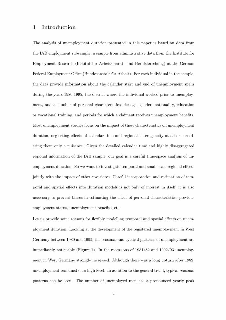
1 Introduction

The analysis of unemployment duration presented in this paper is based on data from

the IAB employment subsample, a sample from administrative data from the Institute for

Employment Research (Institut fur Arbeitsmarkt- und Berufsforschung) at the German

Federal Employment Office (Bundesanstalt fur Arbeit). For each individual in the sample,

the data provide information about the calendar start and end of unemployment spells

during the years 1980-1995, the district where the individual worked prior to unemploy-

ment, and a number of personal characteristics like age, gender, nationality, education

or vocational training, and periods for which a claimant receives unemployment benefits.

Most unemployment studies focus on the impact of these characteristics on unemployment

duration, neglecting effects of calendar time and regional heterogeneity at all or consid-

ering them only a nuisance. Given the detailed calendar time and highly disaggregated

regional information of the IAB sample, our goal is a careful time-space analysis of un-

employment duration. So we want to investigate temporal and small-scale regional effects

jointly with the impact of other covariates. Careful incorporation and estimation of tem-

poral and spatial effects into duration models is not only of interest in itself, it is also

necessary to prevent biases in estimating the effect of personal characteristics, previous

employment status, unemployment benefits, etc.

Let us provide some reasons for flexibly modelling temporal and spatial effects on unem-

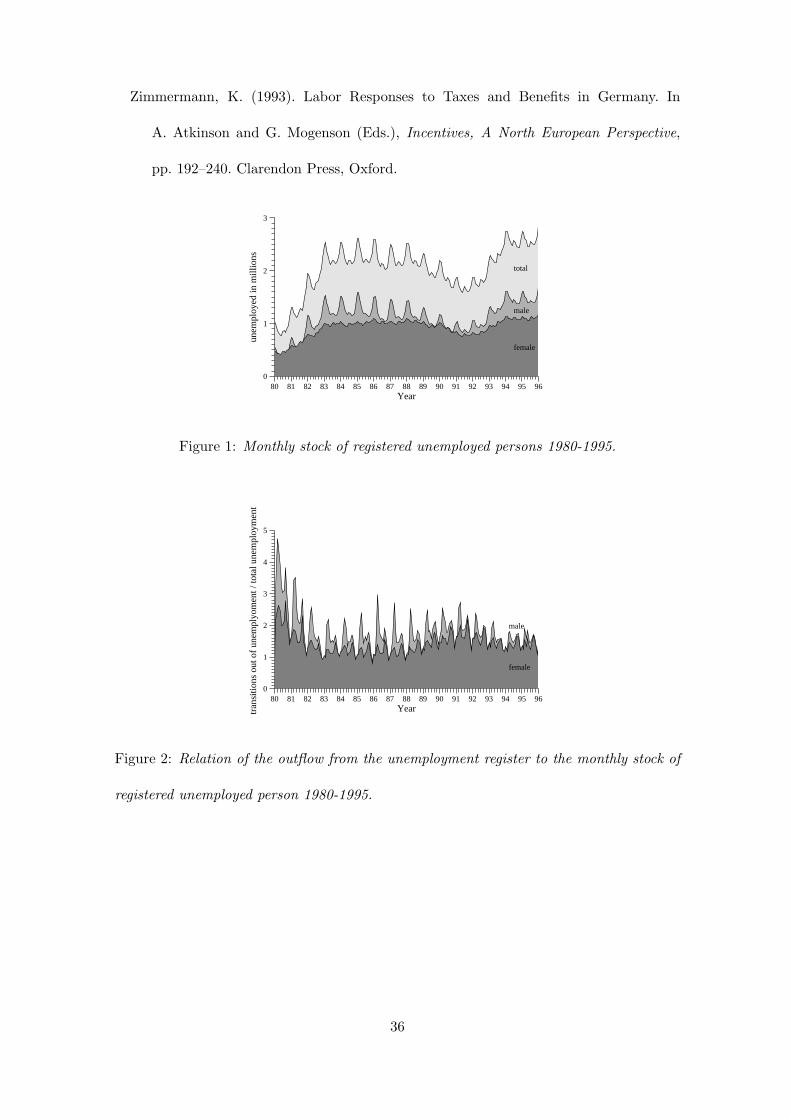
ployment duration. Looking at the development of the registered unemployment in West

Germany between 1980 and 1995, the seasonal and cyclical patterns of unemployment are

immediately noticeable (Figure 1). In the recessions of 1981/82 and 1992/93 unemploy-

ment in West Germany strongly increased. Although there was a long upturn after 1982,

unemployment remained on a high level. In addition to the general trend, typical seasonal

patterns can be seen. The number of unemployed men has a pronounced yearly peak

2

in December. A small rise of the unemployed male population appears in the summer

months. For women there is not such a great peak during the winter months, so that the

”summer high” is just as pronounced as the ”winter high”.

The transitions from unemployment into work also depend on cyclical and seasonal effects

(Schmidt, 1999). The outflow rates from unemployment are plotted against time in Figure

2. During the two recessions the fluctuation out of unemployment decreases. For males

there is an absolute seasonal peak in spring and a smaller one in autumn. For females we

also observe seasonal peaks in autumn and in spring, but only the peak in spring is nearly

as large as for men. The seasonal pattern of the transitions out of unemployment is hence

inverse to that for the stocks in Figure 1.

The monthly stock of persons receiving unemployment benefits shows similar temporal

behaviour. Consequently, trend and seasonal effects of calendar time have to be adequately

incorporated into duration models of unemployment.

Regional differences in unemployment rates and durations are a well known fact, too. In

West Germany there are some regions with sunset industries (e.g., the Saar and the Ruhr

area), that are characterised by considerable structural adjustment. As a general trend

for West Germany, a so-called north-south divide exists, with particularly low unemploy-

ment rates for Bavaria and Baden-Wurttemberg. In addition to this overall pattern, there

are further local spatial effects in special regions, often caused by high or low economic

activity due to concentration effects. Firms of the same region are specialized in the same

industry and use the advantages of a joint regional labor-force pool, the availability of

intermediate products, the technological spill-over effects and the easy transfer of infor-

mation by personal contacts. Though regional aspects of the labor market are investigated

by various authors (for example, Moller, 1995, Borsch-Supan, 1990), regional effects have

not been adequately included in unemployment duration models. Apart from method-

3

ological problems, a main reason has also been the lack of available small-scale regional

information in many unemployment data sets such as the German Socio-economic Panel

(GSOEP). In contrast, our IAB employment sample includes identifiers for small regional

units. Therefore, we develop a model that allows to incorporate spatial effects on durations

of unemployment where correlations among regions are considered appropriately.

Typical methodological questions that arise in such a study are: How can we include and

estimate trends and seasonal components of calendar time in duration models without

imposing too restrictive and rigid parametric forms, instead allowing the same flexibility

as with modern semiparametric methods for Gaussian time series data such as state space

modelling, local regression or spline smoothing? Can calendar time effects and duration

time effects be analyzed jointly, that is how can multiple time scales be incorporated?

Are there nonlinear effects of metrical covariates, for example age? How can we include

regional effects of districts or labor market regions and account for spatial correlation with

neighbouring districts? It is obvious that complex models are needed for simultaneously

analyzing these questions.

Traditional parametric duration models are not flexible enough for exploring and answering

these questions. Without any rather informative prior knowledge about specific forms of

nonlinear or spatial effects, a very large number of parameters has to be introduced, making

estimation either very unreliable or even impossible due to divergence or nonexistence

of estimates. In this situation, non- or semiparametric approaches that do not assume

certain parametric forms of various nonlinear, temporal and spatial effects, are needed.

More parsimonious parametric forms may then be postulated in a second step.

In this paper, we use a semiparametric Bayesian method that allows a unified treatment

of multiple time scales, linear and nonlinear effects of covariates and of spatially corre-

lated random effects. It has been developed in the context of generalized additive mixed

4

regression models in Fahrmeir and Lang (2001a, b) and Lang and Brezger (2001). Since

unemployment duration is measured in months, we choose discrete-time duration mod-

els. In this paper we model only the transition of leaving unemployment for full-time

employment. The approach is an extension of dynamic discrete-time duration models

developed in Fahrmeir and Wagenpfeil (1996) and Fahrmeir and Knorr-Held (1997) to

models with multiple time scales and unstructured or spatial random effects. Inference

is done through recent Markov chain Monte Carlo simulations. We prefer this Bayesian

method to more conventional semiparametric methods like spline smoothing via penalized

likelihood (Hastie and Tibshirani, 1990) or local regression (Fan and Gijbels, 1996) for the

following reasons:

(i) In contrast to the latter methods, spatial effects can be conveniently modelled and

estimated using Markov random field priors.

(ii) Estimation of unknown smoothing parameters is automatically incorporated.

(iii) No approximations based on asymptotic normality assumptions or conjectures have

to be made.

(iv) MCMC simulation techniques provide a rich output for flexible and sophisticated

inference based on posterior samples.

(v) Predictive distributions can be computed without ”plug in” methods.

After some descriptive statistics and preliminary exploratory data analysis in Section 2,

we apply the Bayesian semiparametric method outlined in Section 3 for a space-time

analysis of unemployment duration in West Germany from 1980-1995. The analyses are

carried out separately for men and women since they show different behaviour on the

labor market under several aspects. The results provide some new and refined insights

5

compared to previous studies. In particular, effects of time and space can be investigated

more thoroughly.

2 Descriptive and exploratory examination of the data

2.1 The IAB employment sample

Our analysis is based on official register data from the German Federal Labor Office,

the so-called IAB employment subsample. It covers the years 1975 to 1995. A detailed

description of the IAB employment subsample can be found in Bender et al. (2000). The

sample contains data of one percent of all employees registered by the social insurance

system within the given period of 21 years. Supplementary information on establishments

and on unemployment periods in which a claimant received benefits is added to the sample.

This version contains exact daily employment history of persons as recorded by the social

insurance system and on periods of benefit receipt (unemployment benefit, unemployment

assistance and maintenance or subsistence allowance). The basis of the IAB employment

subsample is the integrated notifying procedure for health insurance, statutory pension

scheme and unemployment insurance. The procedure requires that employers report all

information of their employees registered by the social security system to the social security

agencies. Hence, the data set allows to reproduce employment careers without the typical

problems of longitudinal surveys arising in social research (e.g. panel mortality, memory

gaps). Compared to unemployment spell data from the GSOEP, the data set covers

a longer observation period and is much larger. Moreover, recordings on duration and

calendar time of unemployment spells are more reliable, since they are not based on

retrospective interviews. Thus, no heaping should arise (Kraus and Steiner 1998).

The IAB employment subsample includes workers, salaried employees and all trainees, as

6

long as they are not exempt from the obligation to pay social insurance contributions.

The characteristics sex, year of birth, nationality, marital status, number of children and

qualifications, are collected for each employee recorded by social insurance. The data on

employment contains information on the occupational code, the occupational status, the

gross earnings, an establishment number issued by the Employment Service, the industry

and the size of the establishment. In the annual averages, the IAB employment subsample

includes about 200000 people in Western Germany.

The IAB employment subsample is usually only available in an anonymised version. One

of the anonymisation procedures is a shift of the complete employment history of each

person on the calendar time axis. This may destroy the seasonal pattern, so we use the

original version of the data set. Small-scale regional information is given by the district

where employed persons works, but is only available in the original version, too.

2.2 The sample of unemployment benefit recipients

Our analysis will be based on a subsample of unemployment benefit recipients of West

Germany excluding West-Berlin from 1980 to 1995. Only the transition from unemploy-

ment to full-time employment will be analyzed. Men and women are always considered

separately, since different behaviour on the labor market has to be expected. Only persons

receiving benefits are included.

We now state some basic facts about the German unemployment benefits scheme needed

later. It distinguishes between unemployment insurance benefit and unemployment as-

sistance. To be eligible for unemployment insurance benefit, the applicant must have

contributed for at least 12 months over the preceding three years to the unemployment

insurance scheme. Unemployment insurance benefits can be received for up to 32 months

(since July 1987), with the duration of the entitlement period depending on age and the

7

length of contributions to the scheme. If unemployment insurance benefit is exhausted,

or if the employee is not eligible for unemployment insurance benefit, he can claim unem-

ployment assistance, which are means-tested. More details on the German compensation

scheme can be found in Zimmermann (1993).

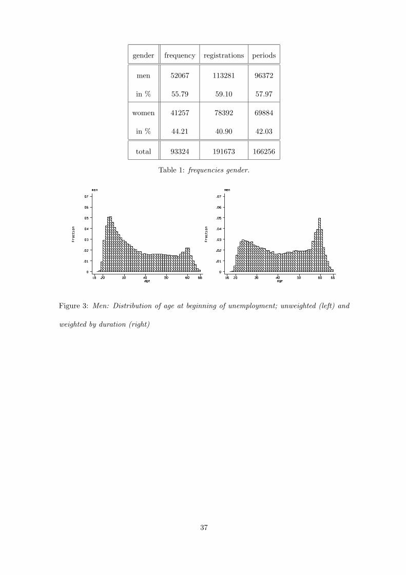
Table 1 shows absolute and relative frequencies of men and women, and of the numbers of

unemployment periods and registrations, stratified by gender. Unemployment periods are

defined by beginning and end of unemployment. Since additional registration of certain

events like change of unemployment benefits can occur within a period, the number of

registrations is higher than the number of periods. We note that there are about 59%

male and 41% female registrations in the data set, and about 58% and 42% unemployment

periods of men and women, respectively. The number of spells is lower than the number

of people in the sample, since some people became unemployed for several times over the

observation period.

Figures 3 and 4 display the age distribution of unemployment registrations for each gen-

der, separately. The figures on the left display these distribution without weighting for

the duration of unemployment. The distribution peaks for both men and women in their

early/mid 20s and then decreases considerably until their late 30s. Each age cohort be-

tween 40 and 55 years makes up for a low percentage (somewhat less than 2 percent) of

the sample. For age cohorts of people aged 55 to 60 years this proportion is not much

higher. It becomes extremely low for cohorts above the age of 60. However, these distri-

butions did not reflect the duration of unemployment. So let us see how much the age

cohorts contribute to the sample in terms of spell length. We display the age distribution

of the registrations weighted by their unemployment duration on the right-hand side of

the Figures 3 and 4. Both for men and women these distributions differ a lot from the

unweighted distributions: Men in their mid 20s now contribute much less to the sample,

8

since their spell lengths are relatively short, while men aged 55 to 60 make up for a much

larger share as they face particularly long unemployment spells. The weighted age distri-

bution of women differs in a similar way from the unweighted one, though the differences

are less pronounced.

This is in agreement with mean duration of unemployment periods classified by gender

and age groups in Table 2. It becomes obvious that the younger ones, although more

often unemployed, leave unemployment or change jobs significantly faster, while older

unemployed have problems of finding a new job or perhaps rely on financial support from

employers or the social security system and wait for early retirement.

Table 3 contains the percentages of unemployment spells cross-classified by gender and

nationality. The share of foreigners is about 12% for men and 10% for women.

Figure 5 shows the distribution of the two categories of unemployment benefits for men and

women. A small share of men and women receive unemployment assistance, while roughly

80 percent receive unemployment insurance. The latter share is higher for women than

for men, while the opposite is true for the share of unemployment assistance recipients.

This could be explained by the fact that women are more inclined to become a housewife

after a period of unemployment with support from unemployment insurance.

Figure 6 displays the mean duration of unemployment for men and women in the fed-

eral states of West Germany. The horizontal straight line marks the overall mean. This

indicates heterogeneity, which will be analyzed in more detail in Section 4. For males,

lower mean durations in Bavaria (BAY), Baden-Wurttemberg (BW) and Rheinland-Pfalz

(RLP) and higher mean durations in Saarland (SAL), Nordrhein-Westfalen (NRW), Bre-

men (BRE) and Hamburg (HAM) seem to be consistent with the so called north-south

divide. For females, however, this regional heterogeneity pattern is less pronounced.

Similarly Figure 7 displays the average duration of unemployment for different sectors of

9

the economy. Particularly striking is the low mean duration for the agricultural sector and

for construction (for men only), probably caused by a large share of seasonally unemployed

workers. There are also obvious differences between men and women in the sectors energy

(including water supply and mining), construction and social service. Again, duration of

unemployment by sector varies less for women than for men.

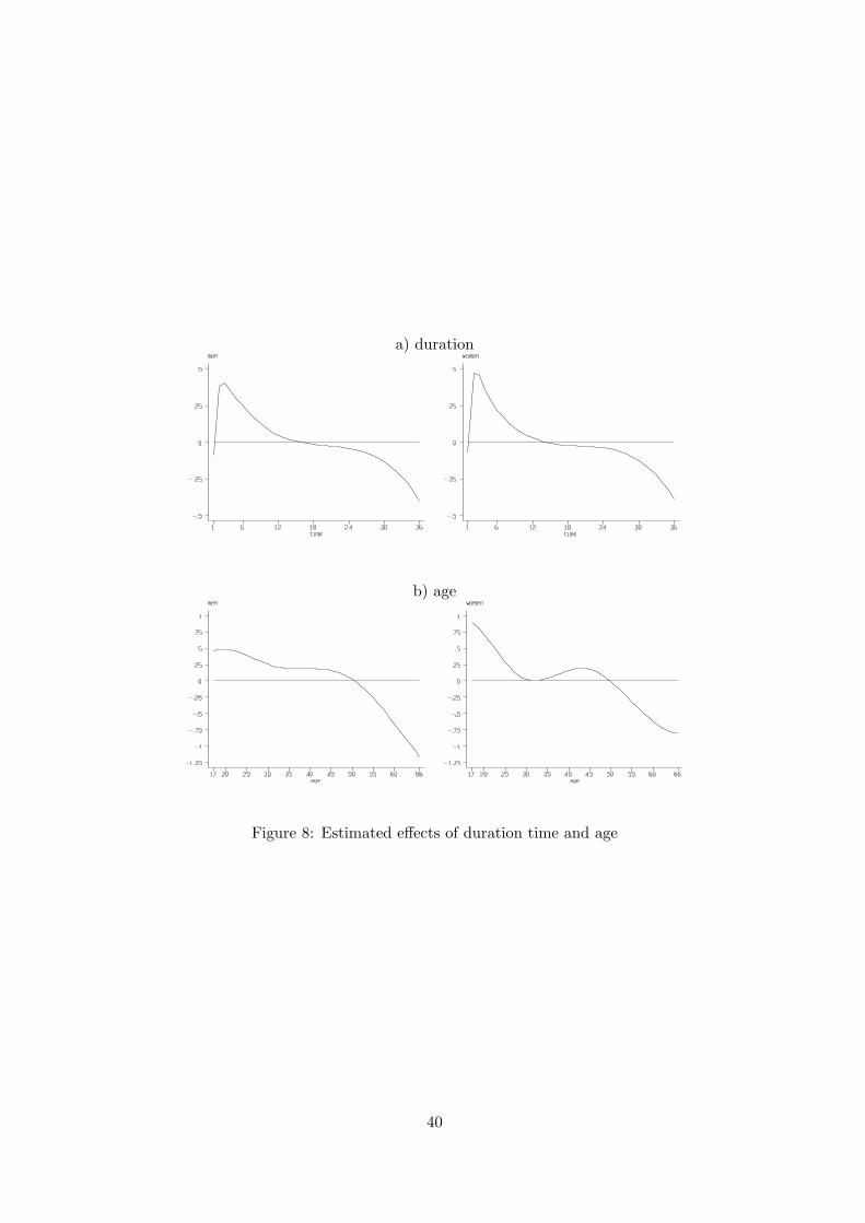
A first exploratory data analysis using STATA was carried out with a parametric probit

model for the probability of leaving unemployment. The effects of duration time and age

were modelled as smooth functions by cubic regression splines with two carefully selected

knots, while calendar time was included in categorized form with a fixed seasonal pattern.

Covariates like nationality, unemployment benefits etc. entered the model in effect coding.

Figure 8 gives a first impression of the effects of duration time and age. While the effect

of duration of the current unemployment spell looks rather similar for men and women,

age effects show some difference but reflect the descriptive finding described before quite

well.

Though simple parametric models are useful for a first analysis, specification of more

complex models including unknown functional forms of duration time, calendar time and

spatial effects as well as other continuous covariates like age is usually difficult if not

impossible. Already for the simple probit model above, fitting of nonlinear effects of

duration time and age requires a careful choice for the number and location of knots.

With only a small number of knots, location of the knots has great influence on the

fitted functional form. For the fitted curves in Figures 7 and 8, knots where chosen as

quantiles to assure that about the same number of observations lies in each of the intervals

defined by the knots. With more nonlinear functions, like trend and seasonal component

of calendar time, and with the inclusion of effects of different sectors of the economy and a

large number of spatially correlated effects of countries or districts, such a ”fixed effects”

10

parametric approach is not feasible. The next section describes a flexible semiparametric

Bayesian approach for data analysis with more complex models.

3 Semiparametric Bayesian modelling and estimation of

discrete-time duration models

3.1 Observation model

Since duration of unemployment as well as calendar time are measured in months, we use a

discrete-time duration model, as described for example in Fahrmeir and Tutz (2001, Ch.9).

Let the discrete duration time D ∈ {1, . . . , d, . . .} denote the end of duration in month d

after beginning of unemployment. In addition to duration D, a sequence of possibly time-

varying covariate vectors xd = (xd1, . . . , xdk) is observed. Let x∗d = (x1, . . . , xd) denote the

history of covariates up to month d. Then the discrete hazard function is given by

λ(d, x∗d) = P (D = d|D ≥ d, x∗

d), d = 1, 2, . . . ,

that is the conditional probability for the end of duration being in interval d, given the

interval is reached and given the history of covariates.

In economic terms, the hazard may be regarded a reduced form of the neoclassical job

search model (Kiefer, 1988). It represents the product of the probability that an unem-

ployed person receives a job offer (arrival rate, α) and the probability that this person

accepts it. The latter is the probability that the offered wage (w) exceeds the individuals

reservation wage (wr)

λ(d, x∗d) = α(1 − F (wr))

where F (w) represents the distribution function of the wage offers.

For a sample of individuals i, i = 1, . . . , n, let Di denote duration times and Ci right

11

censoring times. Duration data are usually given by (di, δi, x∗idi

), i = 1, . . . , n, where

di = min(Di, Ci) is the observed discrete duration time, δi = 1 if Di < Ci, δi = 0 else,

is the censoring indicator, and x∗idi

= (xid, d = 1, . . . , di) is the covariate sequence. We

assume that censoring is noninformative and occurs at the end of the interval, so that the

risk set Rd includes all individuals who are censored in the interval d.

We define binary event indicators yid, i ∈ Rd, d = 1, . . . , di, by

yid =

⎧⎪⎪⎪⎨⎪⎪⎪⎩

1 if d = di and δi = 1

0 else.

For i ∈ Rd, the hazard function for individual i can then be modeled by binary response

models

pr(yid = 1|x∗id) = h(ηid), (1)

with appropriate predictor ηid and response function h : R → (0, 1). In other words,

we model the conditional probability of leaving unemployment, given current duration d

of unemployment in months, calendar time t, the region where the unemployed worked

before, and other, possibly time-varying covariates. Common choices for binary response

models are the grouped Cox model and probit or logit models. We prefer a probit model,

because in this case the binary response model (1) can be written equivalently in terms of

latent Gaussian utilities

Uid = ηid + εid

with Gaussian errors εid ∼ N(0, 1). Following the principle of random utility, yid = 1 is

equivalent to Uid > 0 and yid = 0 is equivalent to Uid < 0. We will see below that the

formulation of the model in terms of latent Gaussian utilities can be utilized for estimation

leading to very efficient estimation algorithms.

The traditional form of the predictor is

ηid = f1(d) + z′idγ, (2)

12

where the sequence f1(d), d = 1, 2, . . . , of parameters represents the baseline effect, and

the design vector zid is some appropriate function of covariates. In general, nonparametric

modelling of the function f1(d) will be required to detect and explore unknown patterns of

the baseline hazard. Then (1) and (2) can be considered as the basic form of a semipara-

metric predictor. In many applications however, additional flexibility is needed to account

for nonlinear or time-varying covariate effects and, as in our application, for further time

scales, such as trend and season in calendar time, and for spatial effects of districts or

labor market regions.

Based on the results of Section 2, we extend the predictor (2) to a more general semipara-

metric form by including effects of calendar time t, of the metrical covariate age a at the

beginning of unemployment and of the labour market region s, where the unemployed has

his/her domicile. This leads to a predictor of the form

ηid = f1(d) + f2(ai) + fT3 (tid) + fS

4 (tid) + f5(si) + z′idγ. (3)

Here f2(a) is a possibly nonlinear effect of age a, fT3 and fS

4 are a decomposition of

the effect of calendar time into a time trend and seasonal component, f5 represents the

effect of labour market regions, and the term z′idγ contains the usual fixed effects of

mostly categorical covariates, such as nationality, education, indicators for entitlement to

unemployment benefits, etc. Note that calendar time is formally treated like a time-varying

covariate.

Models with predictor (3) form the basis of our analysis. Therefrom we will discuss

several extensions based on the varying coefficients framework introduced by Hastie and

Tibshirani (1993). Here, the effect of a particular covariate z, say, is assumed to vary

smoothly over the range of a second covariate x leading to a predictor of the form

η = · · · + f(x)z + · · · .

13

In other words, the term f(x)z models an interaction between z and x. Covariate x

is called the effect modifier of z. In a first extension of our basic model (3) the varying

coefficients framework is used to model possible time-space interactions. More specifically,

we subdivide calendar time into the two distinct intervals 1980 to 1990/6 and 1990/7 to

1995 and define the indicator variable t90/7−95 whose values are one if an observation falls

into the particular time period and zero otherwise. The two intervals are chosen such that

we may identify possible structural breaks due to the German unification. A time space

interaction is then modelled by a predictor of the form

ηid = . . . + fT3 (tid) + fS

4 (tid) + f5(si) + f6(si)t90/7−95id + · · · .

The function f5 corresponds now to the regional effect for the time period between 1980

and 1990/6, and f6 can be considered as deviations from the effect in the first time

period. More details can be found in Section 4.2. A second extension is based on similar

methodology, see Section 4.3.

3.2 Prior assumptions

From a classical perspective, unknown functions f1(·), f2(·), f3(·) and f4(·) as well as the

effects γ = (γ1, . . . , γr) are considered as fixed and unknown, while f5(s) s = 1, . . . , S

is considered as a spatially correlated random effect. Therefore the model (3) together

with the binary response model (1), define a generalized additive mixed model (GAMM).

Conventional non- or semiparametric methods like spline smoothing or local regression

allow flexible modelling and estimation of the functions fj(·), j = 1, 2, 3, 4 together with

fixed effects γ, but are far less developed for GAMM’s, where random effects, in particular

correlated spatial random effects, are included.

In a Bayesian approach, as the one we will follow, all functions, more exactly the vectors

f1 = {f1(d), d = 1, 2, . . .}, f2 = {f2(a), a = 1, 2, . . .} etc. of function evaluations and

14

parameters γ = (γ1, . . . , γr) are considered as random variables. The observation model

(1) together with (3), is understood as conditional upon these random variables, and has

to be supplemented by appropriate prior distributions. For the fixed effect parameters,

we will usually assume independent diffuse priors

p(γj) ∝ const, j = 1, . . . , r.

Another choice would be highly dispersed Gaussian priors.

Priors for the unknown functions fj depend upon the type of covariate. We will distinguish

between metrical covariates, time scales and spatial covariates.

Consider first the effect of a metrical covariate like age a. For the moment we may

distinguish roughly two main approaches for Bayesian semiparametric modelling. These

are base functions approaches with adaptive knot selection (e.g. Denison et al., 1998

, Biller, 2000 and Smith and Kohn, 1996) and approaches based on smoothness priors.

In the following we will focus on the latter one. Several alternatives are possible for

specifying a smoothness prior for the effect of a metrical covariate. Among others, these

are random walk priors (Fahrmeir and Lang, 2001a), Bayesian smoothing splines (Hastie

and Tibshirani, 2000) and Bayesian P-splines (Lang and Brezger, 2001). In the following

we will focus on P-splines. The basic assumption behind the P-splines approach is that an

unknown smooth function f of a particular covariate x can be approximated by a spline of

degree l defined on a set of equally spaced knots ζ0 = xmin < ζ1 < . . . < ζr−1 < ζr = xmax

within the domain of x. It is well known that such a spline can be written in terms of a

linear combination of m = r + l B-spline basis functions Bt, i.e.

f(x) =m∑

t=1

βtBt(x).

The Basis functions Bt are defined locally in the sense that they are nonzero only on

a domain spanned by 2 + l knots. It would be beyond the scope of this paper to go

15

into the details of B-splines and their properties, see e.g. de Boor (1978). The vector

β = (β1, . . . , βm) is unknown and must be estimated from the data. In a simple regression

spline approach the unknown regression coefficients are estimated using standard methods

for fixed effects parameters. However, a crucial point with simple regression splines is the

choice of the number and the position of knots. For a small number of knots the resulting

spline space may be not flexible enough to capture the variability of the data. For a large

number of knots estimated curves may tend to overfit the data. As a remedy to these

problems Eilers and Marx (1996) suggest a moderately large number of knots (usually

between 20 and 40) to ensure enough flexibility, and to define a roughness penalty based

on differences of adjacent regression coefficients to guarantee sufficient smoothness of the

fitted curves. In a Bayesian approach, we replace difference penalties by their stochastic

analogues, i.e. first and second order random walk models for the regression coefficients

βt = βt−1 + ut, βt = 2βt−1 − βt−2 + ut (4)

with Gaussian errors ut ∼ N(0, τ2) and diffuse priors β1 ∝ const, or β1 and β2 ∝ const,

for initial values, respectively. A first order random walk penalizes abrupt jumps βt−βt−1

between successive states and a second order random walk penalizes deviations from the

linear trend 2βt−1 − βt−2. Random walk priors may be equivalently defined in a more

symmetric form by specifying the conditional distributions of parameters βt given its left

and right neighbours, e.g. βt−1 and βt+1 in the case of a first order random walk. Then,

random walk priors may be interpreted in terms of locally polynomial fits. A first order

random walk corresponds to a locally linear and a second order random walk to a locally

quadratic fit to the nearest neighbours, see e.g. Besag et al. (1995).

The amount of smoothness is controlled by the additional variance parameter τ2, which

corresponds to the smoothing parameter in a frequentist approach. The larger (smaller)

the variance, the rougher (smoother) are the estimated functions.

16

Consider now time scales like duration or calendar time. Depending on the particular

situation we may estimate only a nonlinear time trend as for duration time, or may further

split up the effect into a trend and a seasonal component as for calendar time. For the

trend components we can choose the same priors as for metrical covariates. A common

smoothness prior in Gaussian time series analysis for a monthly seasonal component is

fS(t) = fS(t − 1) + . . . + fS(t − 11) = uSt ∼ N(0, τ2). (5)

In contrast to conventional parametric modelling of seasonal effects by dummy variables

for quarters or months, (5) allows for a flexible monthly seasonal pattern that may change

over the years.

Let us now turn our attention to the labour market region indicator s. For the spatial effect

f5(s) = (f5(s), s = 1, . . . , S)′ we choose Markov random field priors common in spatial

statistics (Besag, et al. 1991). These priors reflect spatial neighbourhood relationships.

For geographical data one usually assumes that two sites or regions s and r are neighbours

if they share a common boundary. Then a spatial extension of random walk models leads

to the conditional, spatially autoregressive specification

f5(s)|f5(r), r �= s ∼ N(∑r∈∂s

f5(r)/Ns, τ25 /Ns),

where Ns is the number of adjacent regions, and r ∈ ∂s denotes that region r is a neighbour

of region s. Thus the (conditional) mean of f5(s) is an average of function evaluations

f5(r) of neighbouring regions. Again the variance τ25 controls the degree of smoothness.

For a fully Bayesian analysis, variance or smoothing parameters τ2j , j = 1, 2, . . ., are also

considered as unknown and estimated simultaneously with unknown functions or random

effects. Therefore, hyperpriors are assigned to them in a second stage of the hierarchy by

inverse gamma distributions

p(τ2j ) ∼ IG(aj , bj), j = 1, 2, . . . , .

17

A common choice for aj and bj is very small aj = bj , for example aj = bj = 0.0001 leading

to almost diffuse priors for the variance parameters. An alternative proposed, for example,

in Besag et al. (1995) is aj = 1 and a small value for bj , such as bj = 0.005.

Since the variances τ2j act as smoothing parameters, the degree of smoothness is incor-

porated into a joint model together with other parameters. Posterior estimates for the

smoothness are automatically provided by MCMC simulation. We consider this as a

distinct advantage compared to other semiparametric approaches. For example, with a

regression spline approach as in our explanatory data analysis in Section 2, the number

and location of knots determines the degree of smoothness, and appropriate choice of these

parameters is a delicate and nontrivial issue.

In the following, let f = (f1, f2, . . . , ) τ = (τ2j , j = 1, 2, . . . , ) and γ denote parameter

vectors for function evaluations, variances and fixed effects. Then the Bayesian model is

completed by the following conditional independence assumptions:

(i) For given covariates and parameters observations yid are conditionally independent

(ii) Priors p(fj |τ2j ) are conditionally independent.

(iii) Priors for fixed effects, and hyperpriors for τ2j are mutually independent.

3.3 Bayesian inference

Bayesian inference is based on the posterior

p(f, τ, γ|y) ∝ p(y|f, γ) · p(f |τ) · p(τ) · p(γ)

where the right hand side is defined by the model assumptions.

Posterior means together with confidence intervals and other characteristics are obtained

by drawing samples from the posterior by Markov chain Monte Carlo (MCMC) techniques.

MCMC simulation is based on drawings from full conditionals of blocks of parameters,

18

given the rest and the data. In a direct sampling scheme the vectors fj , j = 1, 2, . . ., of

function evaluations are partitioned into smaller blocks fj [u, v] = (fj(u), . . . , fj(v)) and

Markov chain samples from the unnormalized full conditionals p(fj [u, v]|·) are generated by

Metropolis-Hastings (MH) steps with conditional prior proposals as suggested by Knorr-

Held (1999). Drawings from p(γ|·) can be obtained by MH steps with a random walk

proposal or the weighted least squares proposal of Gamerman (1997). Updating of variance

parameters τ2j is done by Gibbs steps, drawing directly from inverse gamma densities.

Details of the updating scheme is described in Fahrmeir and Lang (2001a). For a probit

model, as considered in this paper, a useful sampling scheme can be developed on the

basis of the latent variable mechanism described above, augmenting the observables yid by

corresponding latent utilities Uid = ηid + εid with Gaussian errors εid ∼ N(0, 1). Posterior

analysis is then based on

p(f, γ, τ, U |y) ∝ p(y|U) · p(U |f, γ) · p(f |τ) · p(τ) · p(γ),

with p(Y |U) =∏i,d

p(Yid|Uid). Compared to the direct sampling scheme, additional draw-

ings from full conditionals for the latent variables are necessary. However, updating of the

utilities Uid is easy and fast, because their full conditionals are truncated standard nor-

mals, i.e. Uid is generated from N(ηid, 1) with mean ηid evaluated at current values fj and

γ, subject to the constraints Uid > 0 for yid = 1 and Uid < 0 for yid = 0. As an advantage,

full conditionals for nonlinear functions and fixed effects parameters become Gaussian,

allowing computationally very efficient Gibbs sampling by updating parameter vectors of

each effect in the model in one large block. Numerical efficiency is guaranteed by applying

Cholesky decompositions for band matrices. The resulting MCMC scheme for generating

posterior samples is then defined by drawing from the following full conditionals:

(i) Update the latent utilities Uid by generating samples from their truncated standard

normal full conditionals.

19

(iii) Function evaluations fj , j = 1, 2, . . . and fixed effects γ are generated from Gaussian

full conditionals.

(iv) Samples for variances τ2j are generated from inverse Gamma full conditionals.

More details on the sampling scheme can be found in Fahrmeir and Lang (2001b).

4 Time-space analysis of unemployment duration in West

Germany

Based on preliminary examination of the data in Section 2, we analyse the spells of men

and women separately. Only persons with full time jobs are considered. Only a small

fraction of individuals is unemployed for more than 36 months. We therefore consider

only durations up to 36 months, longer durations are regarded as censored. Throughout

this section, the probability of leaving unemployment is being specified by probit models.

We first consider a basic model with purely additive effects of space and calendar time

(Section 4.1). Based on the results, we consider a model with time-space interactions

(Section 4.2) and a model that allows a closer look at the effect of previous unemployment

experience (Section 4.3).

4.1 The basic model

For our basic model, we choose a probit model

pr(yid = 1|ηid) = φ(ηid)

for the probability of leaving unemployment at month d, with an additive predictor

ηid = f1(d) + f2(ai) + fT3 (tid) + fS

4 (tid) + f5(si) + z′idγ. (6)

20

We assume cubic P-splines with second order random walk penalties for f1, f2 and fT3 ,

the seasonal prior (5) for fS4 , a Markov random field prior for f5 and diffuse priors for

fixed effects.

The following categorical covariates are included in the vector zit (in effect coding):

• Nationality N:

German, Foreign (reference category)

• Education E:

no vocational training, vocational training (reference category), university degree

• Unemployment Bd (in month d of current unemployment period):

unemployment insurance benefit (reference category), unemployment assistance ben-

efit

• Previous unemployment periods Pt (in month t of calendar time):

0 (reference category), 1 or 2, 3 or more

• Economic sectors:

Agriculture

Manufacturing (reference category).

Energy, water supply and mining

Construction

Trade

Transport and communications

Financial sector

Service industry

21

Non-profit organizations and private households

Territorial authorities and social insurance

Results for Fixed effects

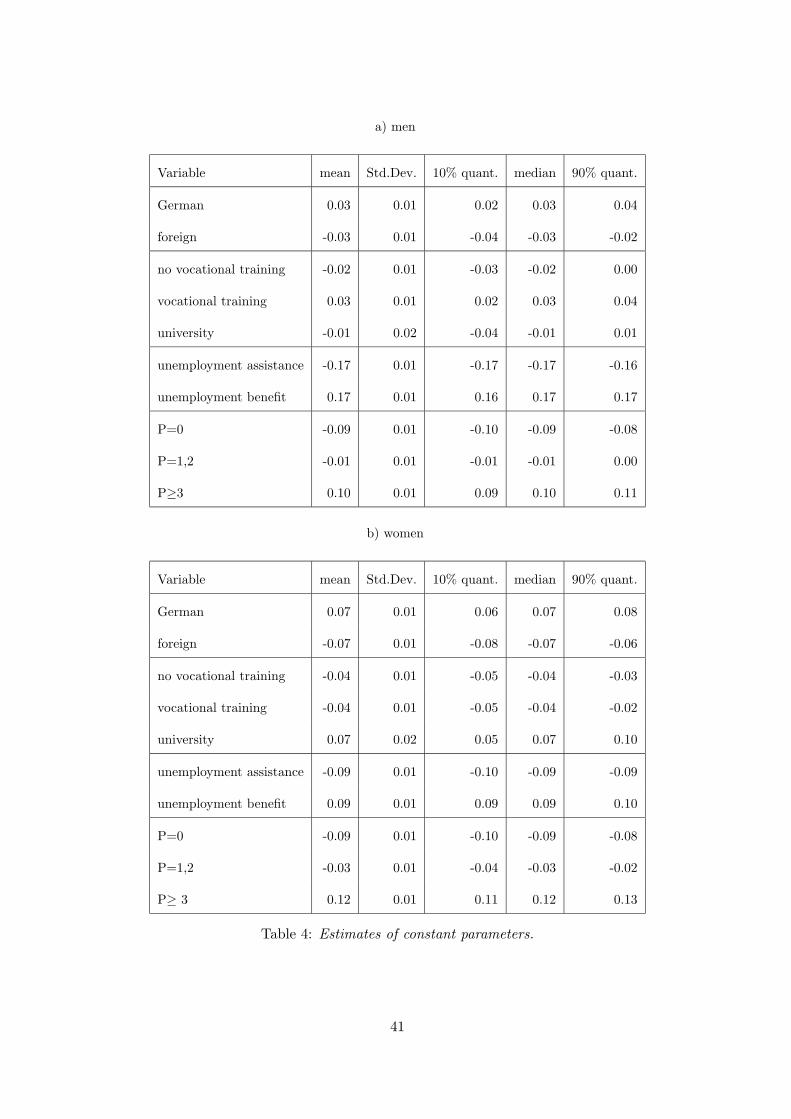
Table 4 contains posterior means, standard deviations, medians and quantiles of fixed

effects of the categorical covariates for men and women, respectively. They confirm some

facts already known from previous analyses with more conventional methods.

Chances for reemployment are better for Germans, and this effect is even stronger for

women. The effect of education differs for men and women: Women with a university

degree have significantly higher reemployment chances compared to women with vocational

training and particularly with no vocational training. For men the effect is insignificant.

A likely explanation is that in contrast to men, for women a higher educational attainment

signals a stronger attachment to the labour market. Thus the higher their human capital,

the more likely they are to stick to their job and so the lower the expected costs of turnover

for the employer. For that reason the arrival rate of job offers may vary positively with

the human capital of women.

The number of previous unemployment periods may signal to employers the (otherwise

unobserved) talents of unemployed people. An adverse performance in the labour market

signals low abilities. Moreover, people who were unemployed many times in the past may

also put less effort into job search than people with no or only a few past unemployment

spells. They may be discouraged as they already did not find suitable jobs in the past.

For both reasons a higher number of past unemployment spells should lead to a lower

arrival rate of job offers and hence has a negative effect on the hazards. However, there

are other considerations that suggest that the opposite may be true: A larger number of

past unemployment periods may increase the need to achieve some earnings and hence

22

reduce the reservation wages of unemployed job searches. Furthermore, the longer peo-

ple have been unemployed in the past the less time they have paid contributions to the

unemployment insurance system prior to their current spell. As the entitlement length

depends positively on this contribution period, a larger number of past unemployment

spells is associated with shorter entitlement lengths to unemployment insurance benefits.

Therefore, a larger number of past unemployment spells may be associated with lower

reservation wages and so a higher probability to accept job offers. Finally, another issue

are workers on recall and/or seasonally unemployed workers. In contrast to other unem-

ployed workers, they regularly loose their jobs so that they are characterised by many past

unemployment spells. Next, they are likely to return to work quickly either to their old

employer or a different employer in the same sector during the next seasonal upturn. This

is another reason to expect a positive association of the number of past spells and the

hazard rate. Our results in the basic model suggest that the hazards rise with the number

of unemployment spells. We investigate in more detail in Section 4.3 whether this is due

to seasonally unemployed workers.

Positive effects of unemployment benefits compared to negative effects of unemployment

assistance are in agreement with findings in previous studies, even with data from the

German Socioeconomic Panel, see Fahrmeir and Knorr-Held (1997). A possible expla-

nation is that individuals with unemployment insurance benefits had regular jobs earlier

and thus get offers for a new job more easily. Next unemployment assistance benefits are

means-tested. Thus the people who receive those benefits are those who are most in need.

These are people who most likely concentrate characteristics that have an adverse impact

on labour market performance. As far as these are unobserved like individual talents,

we would expect the coefficient of the unemployment assistance receipt to pick up their

negative effect on the hazards. Next, while unemployment insurance is paid only for a

23

limited period of time, unemployment assistance may be received indefinitely. So, the

incentives to leave unemployment are lower for the unemployment assistance recipients

than for unemployment insurance recipients.

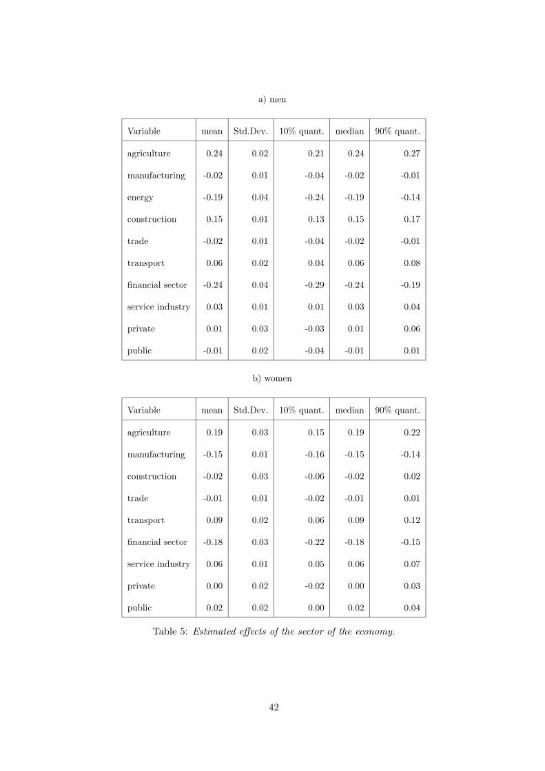
Table 5 shows the effects of economic sectors, where the sector energy, water supply

and mining has been omitted for women, because only a small fraction of women is

working there. There are significant differences between economic sectors. For both

men and women transport and service sectors and particularly agriculture and con-

struction are associated with higher reemployment chances than manufacturing. On the

other side the financial sectors show negative effects for men and, in particular, for women.

Duration dependence effects

Let us first describe some recent findings on duration dependence effects by other authors.

Hujer and Schneider (1996) and Steiner (1997) estimated coefficients of a set of dummies

for the baseline hazard using unemployment spell data of the GSOEP-West. Hujer and

Schneider find the hazards of male unemployment benefit recipients to peak in the fourth

month. They decrease thereafter. Steiner cannot find any negative duration dependence

for the male hazards but for female ones. Our results shed some more light on the issue.

The size of the data set contributes to more precise estimates of the baseline hazard

function. Moreover, in contrast to the studies above the sample size and the specific

semiparametric method allows us to leave the baseline hazard flexible even for duration

times that are longer than one year.

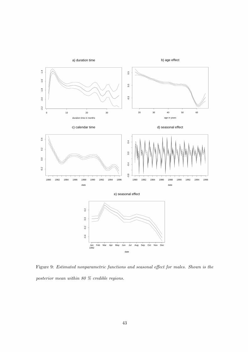
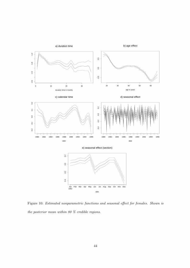
Figures 9 a) and 10 a) plot the estimated nonparametric function of duration. They

demonstrate that the baseline hazards peak in the first two to three months. Thereafter

the hazards tend to fall with duration. The decline is relatively steep up to the tenth

month. Even after ten months of unemployment, the baseline hazards for men and women

24

alike tend to fall. The pattern differs somewhat from other studies on unemployment

duration in Germany. They suggest a negative duration dependence pattern. This may

be due to supply side effects, since unemployed people may become discouraged and

reduce their search effort the longer their spell lasts. It may also be due to demand

side effects: people loose more and more human capital or employers regard long-term

unemployment as an adverse signal of the applicant’s ability. Both is associated with a

lower arrival rate of job offers the longer spells last. This line of reasoning though cannot

explain that the baseline hazard rises considerably during the first two to three months of

duration. Maybe there is a large number of workers on recall in the sample. These may

be mainly seasonally unemployed workers, who are regularly laid off and return after two

to three months of unemployment to their previous employer or an employer in the same

sector. Wolff (1998) showed that a similar peak of the baseline hazard of unemployment

spells in Hungary is mainly caused by such workers.

Age effects

Age should influence the hazards for various reasons. The older a person gets, the shorter

is the time horizon in which he/she may benefit from the offered wage (Fallon and Verry,

1988). So, older workers would have reason to accept more easily a given wage offer than

younger workers. There are other considerations that would lead to opposing conclusions.

For example, if employers invest in firm-specific skills of entrants, they would prefer them

to stay as long as possible in the firm. Therefore, the arrival rate of job offers may decrease

with age. Furthermore, since we include only a limited set of covariates the coefficients of

age most likely capture the effects of some omitted covariates like the number of children

or marital status. This is particularly true for women who do the bulk of housework.

First, the value of one hour household production relative to one hour market work is

25

higher for a mother than for a childless individual, and so is the reservation wage. Second,

institutional constraints as the limited availability of places in creches and kindergardens as

well as their opening hours may adversely affect the hazards of mothers. Third, employers

may be reluctant to hire women, who they regard at risk of becoming mothers, as they

presumably will be less attached to a firm than other workers. So, the arrival rate of job

offers may be very low for the childbearing age-groups.

Figures 9 and 10 b) display the age effects of men and women. The function for men

declines slowly and nearly linearly up to the age of 54. Then it falls rapidly up to the

age 60. Thereafter the hazards rise. The slow linear decline of the hazards with age may

well reflect the fact that employers prefer younger workers to older ones for the reasons

discussed above. However, the age pattern for men older than 54 is certainly related to

institutional rules of retirement for unemployed people. 15 years of waiting time1 and at

least 52 weeks of unemployment during the 18 months before reaching the age of 61 are

necessary to retire already at this age (Lampert, 1998). There is an additional eligibility

criterion of 8 years of contributory employment during the ten year period prior to reaching

the age of 61. So, the incentive of unemployed people to find a job, once they are close

to this retirement age should decrease substantially. This may also explain the increase

in the hazards after the age of 60. Let us consider people who are still unemployed at the

age of 61. These are presumably people who for some reason do not want to retire early

or who do not qualify for an early old age pension. So, their incentives to find a job are

higher than for the average unemployed person who is still a little younger than 61.

Not surprisingly for women older than 50 the age effects are similar to those of men2. In1The waiting time is the sum of years of contributory employment and periods (e.g., military service)

that are treated as equivalent to contributory employment.2Women may retire at the age of 61 even if they have not been unemployed in the 18 months prior to

reaching this age. In order to become eligible, they must have worked in contributory employment for at

26

sharp contrast to men though the hazards of young women decline fairly rapidly until

that age of 30. Between 30 and 50 years, the age function is flat. This pattern is certainly

in line with the hypothesis that the age effect captures the role of children. The likelier it

is that women have children, the lower the hazard. Once that likelihood does not increase

any longer the hazards are relatively stable.

Calendar time and seasonal effects

In the case of women the estimated calendar time effects (Figure 10 c) reflect fairly well

and without much lag the German business cycle. Their hazards are pro-cyclical. We

find a sharp decline in the transition rates to employment of unemployed women at the

beginning of the 80s. They reach their trough at the start of 1983, the year in which the

economy started its upturn. During the first phase of the upturn from 1983 to 1987 GDP

growth never exceeded 3 percent. In that period the hazards increase somewhat. In 1988

GDP growth accelerated. It reached even more than five percent at the beginning of the

90’s as a consequence of the demand shock due to German unification. By that time the

female transition rates increased further and reached their pre-recession levels. The next

downturn started in 1992 and again led to a sharp fall in the transition rates until the

mid of 1993. The following upturn did not last for much longer than one year, so that the

transition rates increased only temporarily.

The male time function (Figure 9 c) declines much more rapidly during the recessions at

the start of the 80s and in 92/93 than that of women. However, the accelerated GDP

growth at the end of the 80s and beginning of the 90s left the male transition rates nearly

unaltered. Presumably there is a negative time trend in the transition rates of men, which

does not characterise that of women. One reason for this may be the general shift of the

least 10 years after reaching the age of 41. Next, a total waiting period of 15 years is required.

27

economy towards service sector and the decline of some industrial sectors like mining and

steel. Male workers who are dismissed in the latter industries even in boom times hardly

find a job in other manufacturing, trade, transport or other service sectors.

Figures 9 and 10 d) display the seasonal effects over the entire observation period. To

gain more insights about the seasonal variation during a single year Figures 9 and 10

e) show a section of the seasonal effects for 1992. For men we observe similar seasonal

patterns year by year. However, the variation of the effects clearly decreased after the

1980’s. In contrast to men, the size of peaks and troughs are much lower for women. This

result is not very surprising, as women less frequently than men work in sectors that are

affected by seasonal demand fluctuations. Moreover, apart from the troughs the seasonal

pattern is less stable over time than for men.

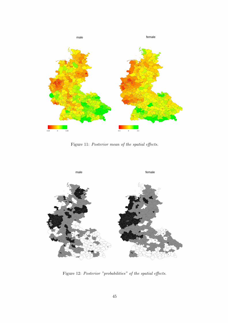
Spatial effects

Estimated posterior means of spatial effects are shown in Figure 11. Since on average

the spatial variation for women is only half of the variation for men we plotted both

maps in different scales, otherwise interpretation of the effects would be difficult. Both

maps show a strong spatial pattern. Chances are improved in the south and become

worse in the middle and the northern part of West Germany. Particularly striking are the

red spots in the west, corresponding to the Saar and the Ruhr area. These regions are

known for their massive structural adjustment problems during the last two decades that

are still ongoing. This becomes even more obvious with Figure 12 showing ”probability

maps”. For a nominal level of 80 % the levels correspond to ”significantly negative” (black

coloured), ”nonsignificant” (grey coloured), i.e. zero is within the credible interval around

the estimate, and ”significantly positive” (white coloured).

28

4.2 Time-space interactions

The basic model (6) allows to specify and to analyze the main effects of calendar time and

labor market regions by an additive decomposition. To investigate non-additive spatio-

temporal effects, interaction terms between calendar time and labor market regions have

to be included. In this section, we specify interaction terms in form of a varying coefficient

model as already mentioned at the end of Section 3.1. The entire observation period is

divided into the two intervals 1980 - 1990/6 and 1990/7 - 1995. The intervals are chosen

such that we may identify structural breaks due to the economic integration and unification

between West-Germany and the former German Democratic Republic. We chose as the

start of this process July 1990, when the German Economic, Social and Monetary Union

came into force.

A model with time-space interaction is then defined by extending (6) to

ηid = f1(d) + f2(ai) + fT3 (tid) + fS

4 (tid)+

f5(si) + f6(si)t90/7−95id + z′idγ,

(7)

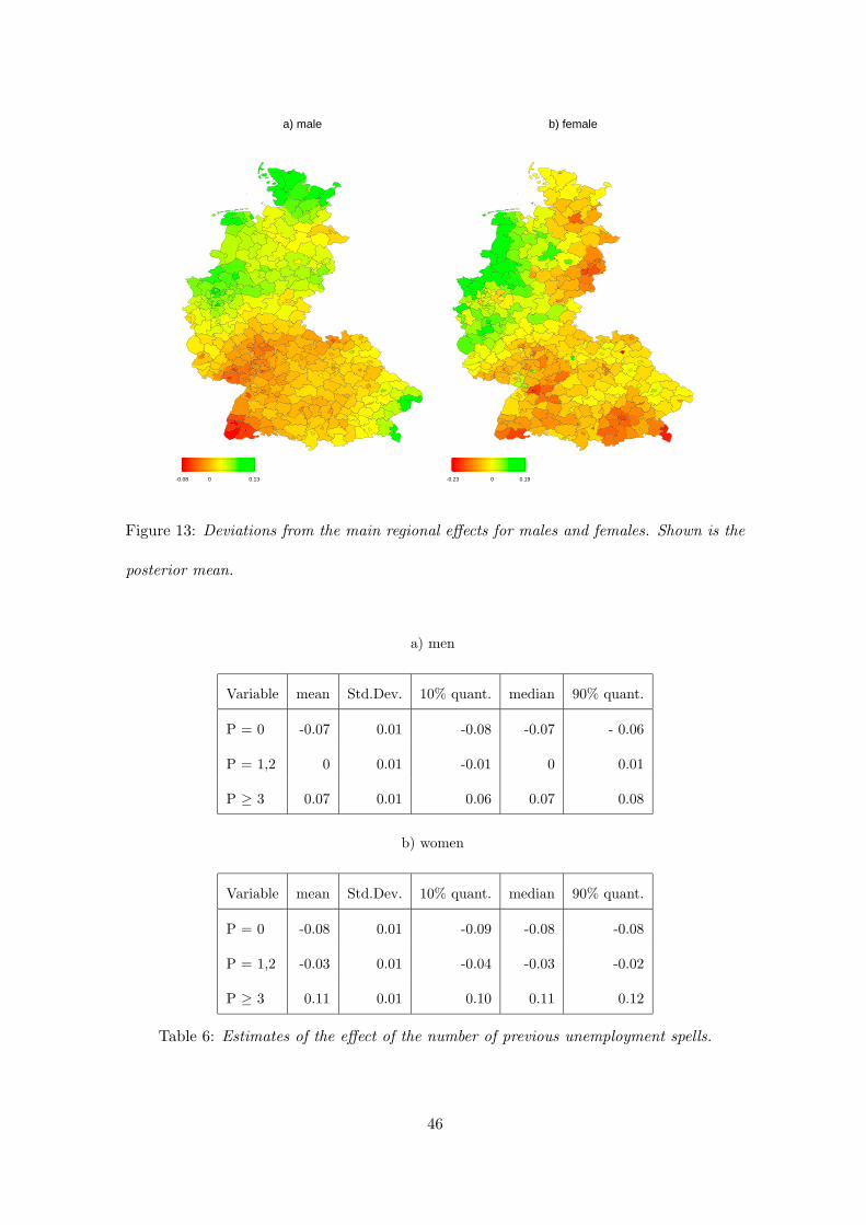
where t90/7−95 is a 0/1 indicator which is 1 for observations after June 1990 and zero

otherwise. The additional spatial effect f6 is the deviation from the main regional effects

f5. These time-space interactions are displayed in Figure 13 for both gender. Note that

these effects do not display whether regions did better or worse than before July 1990.

The reason is that we also modelled a general time trend, which is not reflected in the

figure. The time-space interactions are rather deviations from this general time trend.

Let us first turn to the time-space interactions for men. Figure 13 a) shows an improvement

in male exit to employment for most of the northern regions. The opposite applies to

many of the southern ones. One may expect that the economic integration between West-

and East-Germany had a particular impact on the regions that are close to the former

German Democratic Republic. These are the border regions in the northeast and mideast.

29

However, their performance neither generally worsened nor improved. One reason why

one might have expected an adverse effect for these areas is the high unemployment in the

new federal states that emerged during the transition process. The male unemployment

rate in East Germany achieved a level of more 10 percent in January 1992. Until the

end of 1995 it stayed most of the time above this level. For women in East Germany the

unemployment rate was about twice as high as for men. Next, wages in West-Germany

were considerably higher than in East-Germany. For both reasons East-Germans may have

competed with West-Germans for vacancies in the former border districts. Now regard

Figure 13 b) for women. There is some indication that this competition had an adverse

effect on the hazards. For nearly all districts at the former border between East- and

West-Germany the interaction-effect is below average. It is not very surprising that the

effect occurs for women but not for men. There are male and female dominated segments

in the labour market and female unemployment rates in East Germany were twice as high

as male ones. So, competition for female jobs may have increased far more than for male

jobs in the former border areas.

Estimates of the remaining covariates are practically the same as in the preceding section

and are therefore not presented.

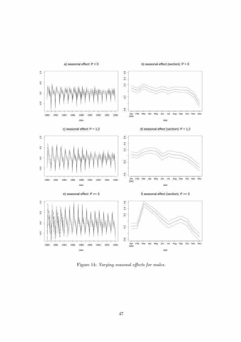
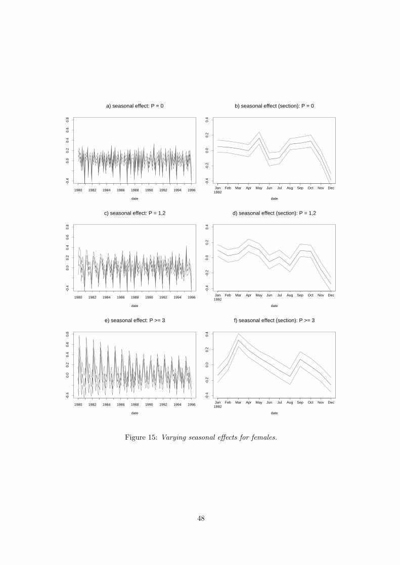
4.3 Seasonality revisited

As already remarked in Section 4.1, the positive effect of higher numbers of previous un-

employment periods may be caused by individuals employed in sectors with high seasonal

effects such as construction or the agricultural sector. To investigate this question, we

modify the influence of seasonal effects in our basic model (6) as follows. We split up

the global additive seasonal component fS4 (t) into three seasonal components interacting

with corresponding categories of the number of previous unemployment periods. Thus,

30

the predictor is now

ηid = f1(d) + f2(ai) + fT3 (tid) + fS1

4 (tid) · P 1i + fS2

4 (tid) · P 2i + fS3

4 (tid) · P 3i

+f5(si) + z′itγ.

Here P 1id, P 2

id and P 3id are 1/0 indicators for the three categories 0, 1 or 2, 3 or more

previous unemployment periods of individual i. The functions fSj

4 (t), j = 1, 2, 3, are

seasonally varying effects of individuals falling into one of these categories. The main

effects for these categories (in effect coding) are still included in the covariate vector zit.

This model allows to investigate if the positive effect of 3 or more previous unemployment

periods is mainly caused by effects of seasonality.

We only report on results for the variable P ”previous unemployment” and the seasonal

components. All other effects remain practically unchanged. The main effects for P are

given in Table 6. They are more or less the same as in the basic model as the hazards

rise with the number of previous spells. This implies that a larger number of previous

unemployment spells is not that much a signal to employers for an adverse performance in

the labour market. The reasons for the result are rather the need of such workers to renew

their eligibility to unemployment insurance benefits and the fact that they are likely to

be on recall. A related argument for such an outcome was that previous unemployment is

also highly associated with seasonal unemployment. Our results for the interaction effects

of the number of previous unemployment spells with seasonality favour this interpretation.

For males and females Figures 14 a-c and 15 a-c show that the seasonality in the hazards

increases considerably, the larger the number of previous spells.

5 Summary and conclusions

This paper presents a Bayesian approach for semiparametric modelling of the dependence

of reemployment chances on covariates with particular emphasis on the spatio-temporal

31

development of the labor market. Our results demonstrate that the approach is a use-

ful and flexible tool for estimating realistically complex models. In contrast to previous

studies on the duration of unemployment in West Germany, our results suggest a negative

duration dependence effect. Besides, the non-parametric estimates of the age effects on

the hazard also provided us with more insights than previous studies like the one of Hujer

and Schneider (1996) or Steiner (1997). These studies and many others model the age

effects by the coefficients of a few dummies representing age-groups or of age-polynomials

of a small degree. By non-parametrically estimating such effects, we can show more clearly

how retirement rules for the unemployed lead to changes in the job exit behaviour, when

unemployed people come closer to the age of retirement. Moreover, we identify a rapid

decline of the hazards with age for women aged younger than 30. This presumably re-

flects that these women become more and more likely to have young children. It may also

reflect that employers are reluctant to offer jobs to these women. Previous studies also

neglected cyclical effects. Our nonparametric estimates of calendar time effects show that

the transition rates to full-time jobs of women are pro-cyclical and follow relatively closely

the economic cycle. This is less so for men.

As has already been mentioned in the introduction, the appropriate consideration of non-

linear effects of time scales, metrical covariates and spatial heterogeneity may be also

important for studies with a different focus. An example are studies about the influence

of unemployment benefits on reemployment chances.

In this paper possible time-space interactions are estimated through varying coefficient

models. However, this approach has some limitations and can be regarded as a first step

for estimating these kind of models. For example, the partition of the observed time period

in the two intervals 1980-1990/6 and 1990/7-1995 is somewhat arbitrary. A more refined

approach could be based on Markov random fields in space and time. Such an approach

32

poses immense computational and methodological challenges. We intend to investigate

this and other possible approaches in future research.

References

Bender, S., A. Haas, and C. Klose (2000). The IAB Employment Subsample 1975-1995.

Opportunities for Analysis Provided by the Anonymised Subsample. IZA Discussion

Paper 177, Bonn.

Besag, J., Y. York, and A. Mollie (1991). Bayesian Image Restoration with two Appli-

cations in Spatial Statistics (with discussion). Annals of the Institute of Statistical

Mathematics 43, 1–59.

Besag, J. E., P. J. Green, D. Higdon, and K. Mengersen (1995). Bayesian Computation

and Stochastic Systems (with Discussion). Statistical Science 10, 3–66.

Biller, C. (2000). Adaptive Bayesian Regression Splines in Semiparametric Generalized

Linear Models. Journal of Computational and Graphical Statistics 12, 122–140.

Borsch-Supan, A. (1990). Regionale und sektorale Arbeitslosigkeit: Durch hohere Mo-

bilitat reduzierbar? Zeitschrift fur Wirtschafts- und Sozialwissenschaften 110, 55–

82.

De Boor, C. (1978). A Practical Guide to Splines. Springer–Verlag, New York.

Denison, D., B. Mallick, and A. Smith (1998). Automatic Bayesian Curve Fitting. Jour-

nal of the Royal Statistical Society B 60, 333–350.

Eilers, P. and B. Marx (1996). Flexible Smoothing using B-splines and Penalized Like-

lihood (with comments and rejoinder). Statistical Science 11, 89–121.

Fahrmeir, L. and L. Knorr-Held (1997). Dynamic Discrete Time Duration Models. So-

ciological Methodology 27, 417–452.

33

Fahrmeir, L. and S. Lang (2001a). Bayesian Inference for Generalized Additive Mixed

Models Based on Markov Random Field Priors. Applied Statistics (JRSS C) 50,

201–220.

Fahrmeir, L. and S. Lang (2001b). Bayesian Semiparametric Regression Analysis of Mul-

ticategorical Time-Space Data. Annals of the Institute of Statistical Mathematics 53,

11–30.

Fahrmeir, L. and G. Tutz (2001). Multivariate Statistical Modelling Based on General-

ized Linear Models (2 ed.). Springer, New York.

Fahrmeir, L. and S. Wagenpfeil (1996). Smoothing Hazard Functions and Time–Varying

Effects in Discrete Duration and Competing Risks. Journal of the American Statis-

tical Association 91, 1584–1594.

Fallon, P. and D. Verry (1988). The Economics of Labour Markets. Phillip Allan Pub-

lishers, Oxford.

Fan, J. and I. Gijbels (1984). Local Polynomial Modelling and Its Applications. Chapman

and Hall, London.

Gamerman, D. (1997). Efficient Sampling from the Posterior Distribution in Generalized

Linear Models. Statistics and Computing 7, 57–68.

Hastie, T. and R. Tibshirani (1990). Generalized Additive Models. Chapman and Hall,

London.

Hastie, T. and R. Tibshirani (1993). Varying-coefficient Models. Journal of the Royal

Statistical Society B 55, 757–796.

Hastie, T. and R. Tibshirani (2000). Bayesian Backfitting. Statistical Science (to ap-

pear).

Hujer, R. and H. Schneider (1996). Institutionelle und strukturelle Determinanten

34

der Arbeitslosigkeit in Westdeutschland: Eine mikrookonometrische Analyse mit

Paneldaten. In B. Gahlen, H. Hesse, and J. Ramser (Eds.), Arbeitslosigkeit und

Moglichkeiten zu ihrer Uberwindung, pp. 53–76. Mohr, Tubingen.

Kiefer, N. (1988). Economic Duration Data and Hazard Functions. Journal of Economic

Literature, 646–679.

Knorr-Held, L. (1999). Conditional Prior Proposals in Dynamic Models. Scandinavian

Journal of Statistics 26, 129–144.

Kraus, F. and V. Steiner (1998). Modelling Heaping Effects in Unemployment Duration

Models - With an Application to Retrospective Event Data in the German Socio-

Economic Panel. Jahrbucher fur Nationalokonomie und Statistik 217, 550–573.

Lampert, H. (1998). Lehrbuch der Sozialpolitik. Springer Verlag, Berlin.

Lang, S. and A. Brezger (2001). Bayesian P-splines. SFB 386 Discussion Paper 236,

University of Munich.

Moller, J. (1995). Empirische Regionalentwicklung. In B. Gahlen, H. Hesse, and

H. Ramser (Eds.), Standort und Region - Neue Ansatze zur Regionalokonomik (Band

24), pp. 197–230. Mohr, Tubingen.

Schmidt, C. (1999). The Heterogeneity and Cyclical Sensitivity of Unemployment: An

Exploration of German Labor Market Flows. IZA Discussion Paper 84, Bonn.

Smith, M. and R. Kohn (1996). Nonparametric Regression using Bayesian Variable

Selection. Journal of Econometrics 75, 317–343.

Steiner, V. (1997). Extended Benefit-Entitlement Periods and the Duration of Unem-

ployment in West Germany. ZEW-Discussion Paper 14, Mannheim.

Wolff, J. (1998). Essays in Unemployment Duration in Two Economies in Transition:

East Germany and Hungary. Ph. D. thesis, Florence.

35

Zimmermann, K. (1993). Labor Responses to Taxes and Benefits in Germany. In

A. Atkinson and G. Mogenson (Eds.), Incentives, A North European Perspective,

pp. 192–240. Clarendon Press, Oxford.

80 81 82 83 84 85 86 87 88 89 90 91 92 93 94 95 960

1

2

3

total

male

female

Year

unem

ploy

ed in

mill

ions

Figure 1: Monthly stock of registered unemployed persons 1980-1995.

80 81 82 83 84 85 86 87 88 89 90 91 92 93 94 95 960

1

2

3

4

5

male

female

Yeartran

sitio

ns o

ut o

f un

empl

yom

ent /

tota

l une

mpl

oym

ent

Figure 2: Relation of the outflow from the unemployment register to the monthly stock of

registered unemployed person 1980-1995.

36

gender frequency registrations periods

men 52067 113281 96372

in % 55.79 59.10 57.97

women 41257 78392 69884

in % 44.21 40.90 42.03

total 93324 191673 166256

Table 1: frequencies gender.

Figure 3: Men: Distribution of age at beginning of unemployment; unweighted (left) and

weighted by duration (right)

37

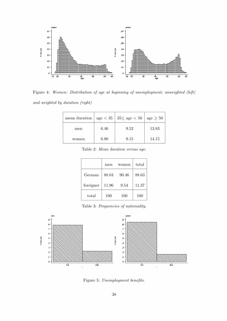
Figure 4: Women: Distribution of age at beginning of unemployment; unweighted (left)

and weighted by duration (right)

mean duration age < 35 35≤ age < 50 age ≥ 50

men 6.46 9.52 13.83

women 6.90 9.15 14.15

Table 2: Mean duration versus age.

men women total

German 88.04 90.46 88.63

foreigner 11.96 9.54 11.37

total 100 100 100

Table 3: Frequencies of nationality.

Figure 5: Unemployment benefits.

38

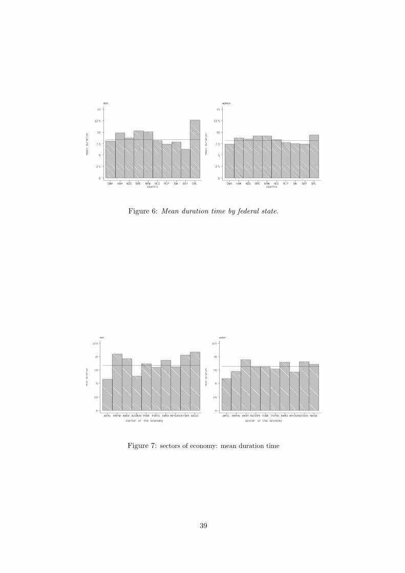
Figure 6: Mean duration time by federal state.

Figure 7: sectors of economy: mean duration time

39

a) duration

b) age

Figure 8: Estimated effects of duration time and age

40

a) men

Variable mean Std.Dev. 10% quant. median 90% quant.

German 0.03 0.01 0.02 0.03 0.04

foreign -0.03 0.01 -0.04 -0.03 -0.02

no vocational training -0.02 0.01 -0.03 -0.02 0.00

vocational training 0.03 0.01 0.02 0.03 0.04

university -0.01 0.02 -0.04 -0.01 0.01

unemployment assistance -0.17 0.01 -0.17 -0.17 -0.16

unemployment benefit 0.17 0.01 0.16 0.17 0.17

P=0 -0.09 0.01 -0.10 -0.09 -0.08

P=1,2 -0.01 0.01 -0.01 -0.01 0.00

P≥3 0.10 0.01 0.09 0.10 0.11

b) women

Variable mean Std.Dev. 10% quant. median 90% quant.

German 0.07 0.01 0.06 0.07 0.08

foreign -0.07 0.01 -0.08 -0.07 -0.06

no vocational training -0.04 0.01 -0.05 -0.04 -0.03

vocational training -0.04 0.01 -0.05 -0.04 -0.02

university 0.07 0.02 0.05 0.07 0.10

unemployment assistance -0.09 0.01 -0.10 -0.09 -0.09

unemployment benefit 0.09 0.01 0.09 0.09 0.10

P=0 -0.09 0.01 -0.10 -0.09 -0.08

P=1,2 -0.03 0.01 -0.04 -0.03 -0.02

P≥ 3 0.12 0.01 0.11 0.12 0.13

Table 4: Estimates of constant parameters.

41

a) men

Variable mean Std.Dev. 10% quant. median 90% quant.

agriculture 0.24 0.02 0.21 0.24 0.27

manufacturing -0.02 0.01 -0.04 -0.02 -0.01

energy -0.19 0.04 -0.24 -0.19 -0.14

construction 0.15 0.01 0.13 0.15 0.17

trade -0.02 0.01 -0.04 -0.02 -0.01

transport 0.06 0.02 0.04 0.06 0.08

financial sector -0.24 0.04 -0.29 -0.24 -0.19

service industry 0.03 0.01 0.01 0.03 0.04

private 0.01 0.03 -0.03 0.01 0.06

public -0.01 0.02 -0.04 -0.01 0.01

b) women

Variable mean Std.Dev. 10% quant. median 90% quant.

agriculture 0.19 0.03 0.15 0.19 0.22

manufacturing -0.15 0.01 -0.16 -0.15 -0.14

construction -0.02 0.03 -0.06 -0.02 0.02

trade -0.01 0.01 -0.02 -0.01 0.01

transport 0.09 0.02 0.06 0.09 0.12

financial sector -0.18 0.03 -0.22 -0.18 -0.15

service industry 0.06 0.01 0.05 0.06 0.07

private 0.00 0.02 -0.02 0.00 0.03

public 0.02 0.02 0.00 0.02 0.04

Table 5: Estimated effects of the sector of the economy.

42

a) duration time

duration time in months

-2.2

-2.0

-1.8

-1.6

-1.4

0 10 20 30

b) age effect

age in years

-0.5

0.0

0.5

20 30 40 50 60

c) calendar time

date

-0.2

0.0

0.2

0.4

1980 1982 1984 1986 1988 1990 1992 1994 1996

d) seasonal effect

date

-0.8

-0.4

0.0

0.4

1980 1982 1984 1986 1988 1990 1992 1994 1996

e) seasonal effect

date

-0.4

-0.2

0.0

0.2

Jan Feb Mar Apr May Jun Jul Aug Sep Oct Nov Dec1992

Figure 9: Estimated nonparametric functions and seasonal effect for males. Shown is the

posterior mean within 80 % credible regions.

43

a) duration time

duration time in months

-2.6

-2.2

-1.8

-1.4

0 10 20 30

b) age effect

age in years

-0.5

0.0

0.5

20 30 40 50 60

c) calendar time

date

-0.2

-0.1

0.0

0.1

0.2

1980 1982 1984 1986 1988 1990 1992 1994 1996

d) seasonal effect

date

-0.4

-0.2

0.0

0.2

1980 1982 1984 1986 1988 1990 1992 1994 1996

e) seasonal effect (section)

date

-0.4

-0.2

0.0

0.2

Jan Feb Mar Apr May Jun Jul Aug Sep Oct Nov Dec1992

Figure 10: Estimated nonparametric functions and seasonal effect for females. Shown is

the posterior mean within 80 % credible regions.

44

0-0.35 0.35

male

0-0.3 0.3

female

Figure 11: Posterior mean of the spatial effects.

male female

Figure 12: Posterior ”probabilities” of the spatial effects.

45

0-0.08 0.13

a) male

0-0.23 0.19

b) female

Figure 13: Deviations from the main regional effects for males and females. Shown is the

posterior mean.

a) men

Variable mean Std.Dev. 10% quant. median 90% quant.

P = 0 -0.07 0.01 -0.08 -0.07 - 0.06

P = 1,2 0 0.01 -0.01 0 0.01

P ≥ 3 0.07 0.01 0.06 0.07 0.08

b) women

Variable mean Std.Dev. 10% quant. median 90% quant.

P = 0 -0.08 0.01 -0.09 -0.08 -0.08

P = 1,2 -0.03 0.01 -0.04 -0.03 -0.02

P ≥ 3 0.11 0.01 0.10 0.11 0.12

Table 6: Estimates of the effect of the number of previous unemployment spells.

46

a) seasonal effect: P = 0

date

-0.5

0.0

0.5

1.0

1980 1982 1984 1986 1988 1990 1992 1994 1996

b) seasonal effect (section): P = 0

date

-0.6

-0.2

0.2

0.4

0.6

Jan Feb Mar Apr May Jun Jul Aug Sep Oct Nov Dec1992

c) seasonal effect: P = 1,2

date

-0.5

0.0

0.5

1.0

1980 1982 1984 1986 1988 1990 1992 1994 1996

d) seasonal effect (section): P = 1,2

date

-0.6

-0.2

0.2

0.4

0.6

Jan Feb Mar Apr May Jun Jul Aug Sep Oct Nov Dec1992

e) seasonal effect: P >= 3

date

-0.5

0.0

0.5

1.0

1980 1982 1984 1986 1988 1990 1992 1994 1996

f) seasonal effect (section): P >= 3

date

-0.6

-0.2

0.2

0.4

0.6

Jan Feb Mar Apr May Jun Jul Aug Sep Oct Nov Dec1992

Figure 14: Varying seasonal effects for males.

47

a) seasonal effect: P = 0

date

-0.4

0.0

0.2

0.4

0.6

0.8

1980 1982 1984 1986 1988 1990 1992 1994 1996

b) seasonal effect (section): P = 0

date

-0.4

-0.2

0.0

0.2

0.4

Jan Feb Mar Apr May Jun Jul Aug Sep Oct Nov Dec1992

c) seasonal effect: P = 1,2

date

-0.4

0.0

0.2

0.4

0.6

0.8

1980 1982 1984 1986 1988 1990 1992 1994 1996

d) seasonal effect (section): P = 1,2

date

-0.4

-0.2

0.0

0.2

0.4

Jan Feb Mar Apr May Jun Jul Aug Sep Oct Nov Dec1992

e) seasonal effect: P >= 3

date

-0.4

0.0

0.2

0.4

0.6

0.8

1980 1982 1984 1986 1988 1990 1992 1994 1996

f) seasonal effect (section): P >= 3

date

-0.4

-0.2

0.0

0.2

0.4

Jan Feb Mar Apr May Jun Jul Aug Sep Oct Nov Dec1992

Figure 15: Varying seasonal effects for females.

48