Signal- und Bildverarbeitung, 323.014 Image Analysis and Processing Arjan Kuijper 30.11.2006

1/31Johann Radon Institute for Computational and Applied Mathematics: www.ricam.oeaw.ac.at

Signal- und Bildverarbeitung, 323.014

Image Analysis and Processing

Arjan Kuijper

30.11.2006

Johann Radon Institute for Computational and Applied Mathematics (RICAM)

Austrian Academy of Sciences Altenbergerstraße 56A-4040 Linz, Austria

[email protected]


Last week

• Total variation minimizing models have become one of the most popular and successful methodology for image restoration.

• ROF (Rudin-Osher-Fatemi) is one of the earliest and best known examples of PDE based edge preserving denoising.

• It was designed with the explicit goal of preserving sharp discontinuities (edges) in images while removing noise and other unwanted fine scale detail.

• However, it has some drawbacks:– Loss of contrast – Loss of geometry – Stair casing– Loss of texture


Today

• Mean curvature motion– Curve evolution– Denoising– Edge preserving– Implementation– Isophote vs. image implementation

Taken from:


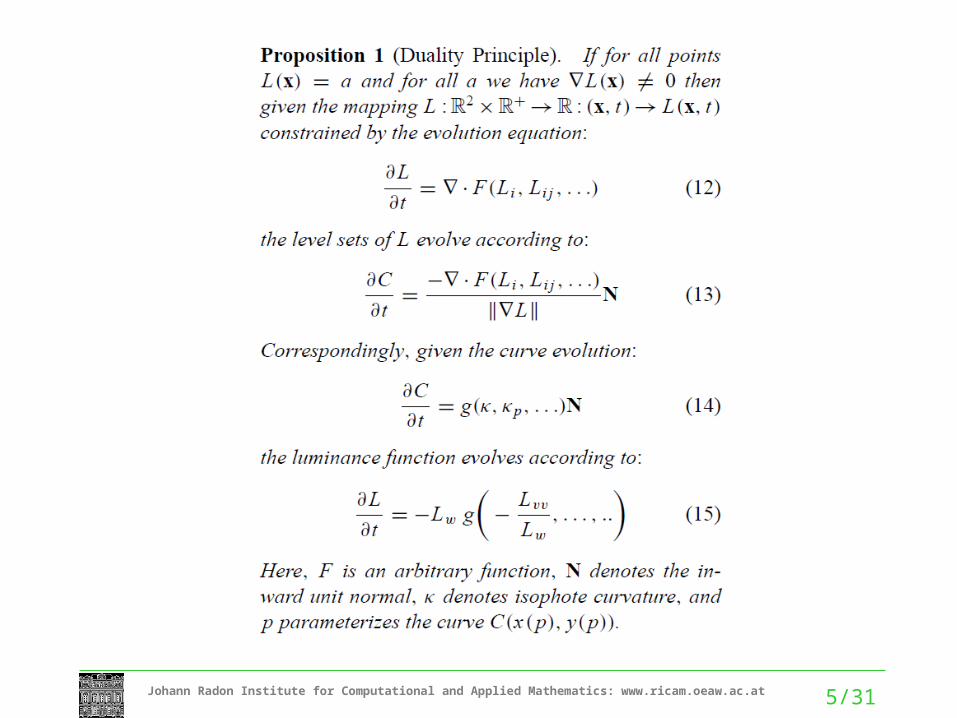
Overview of Evolution Equations

• We start with a generalized framework for a number of nonlinear evolution equations that have appeared in the literature.

• In Alvarez et al. (1993) the interested reader can find an extensive treatment on evolution equations of the general form:

• Imposing various axioms on a multi-scale analysis the authors derive a number of evolution equations that are listed here.

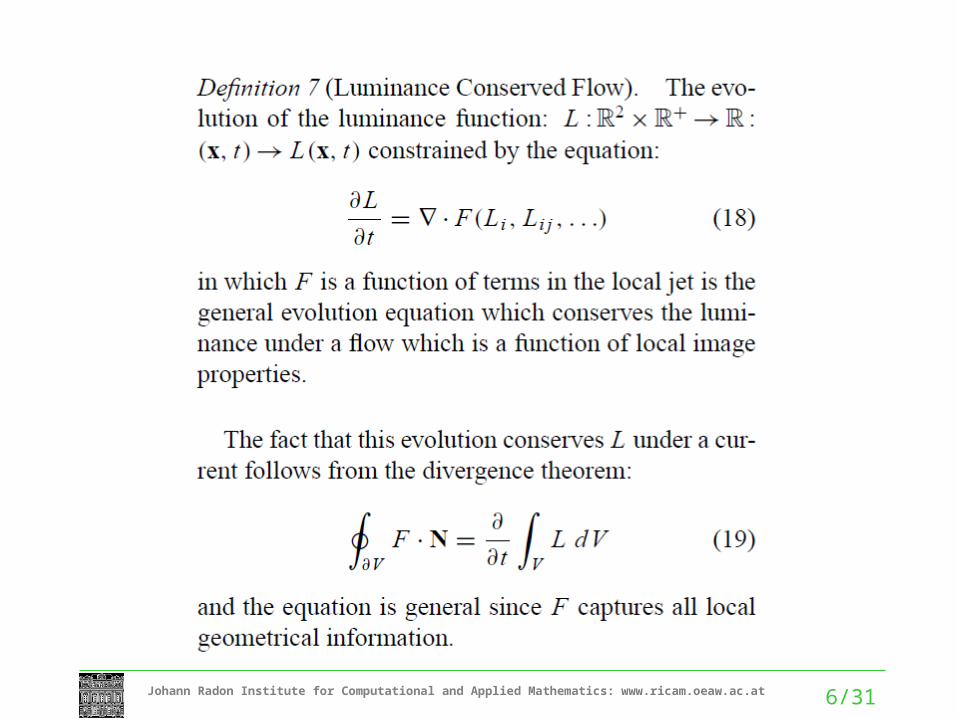
• Here, we distinguish two approaches: – i) evolution of the luminance function and – ii) evolution of the level sets of the image.

• These approaches are dual in the sense that one determines the other

Alvarez, L., Guichard, F., Lions, P.L., and Morel, J.M. 1993. Axioms and fundamental equations of image processing. Arch. for Rational Mechanics, 123(3):199–257.




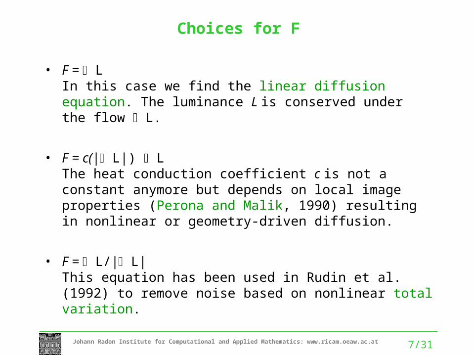
Choices for F

• F = LIn this case we find the linear diffusion equation. The luminance L is conserved under the flow L.

• F = c(| L|) LThe heat conduction coefficient c is not a constant anymore but depends on local image properties (Perona and Malik, 1990) resulting in nonlinear or geometry-driven diffusion.

• F = L/| L|This equation has been used in Rudin et al. (1992) to remove noise based on nonlinear total variation.


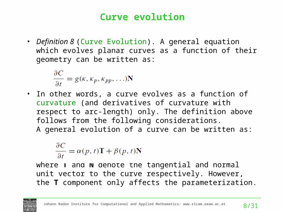
Curve evolution

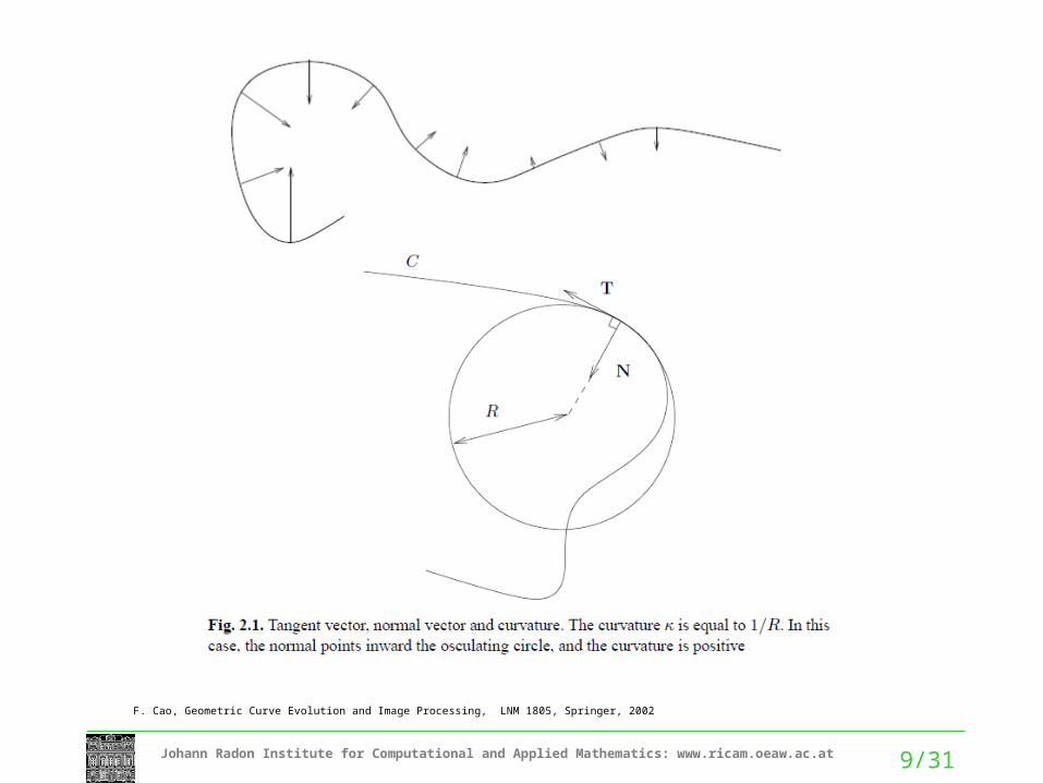
• Definition 8 (Curve Evolution). A general equation which evolves planar curves as a function of their geometry can be written as:

• In other words, a curve evolves as a function of curvature (and derivatives of curvature with respect to arc-length) only. The definition above follows from the following considerations. A general evolution of a curve can be written as:

where T and N denote the tangential and normal unit vector to the curve respectively. However, the T component only affects the parameterization.


F. Cao, Geometric Curve Evolution and Image Processing, LNM 1805, Springer, 2002


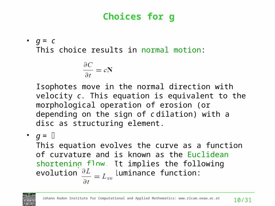
Choices for g

• g = cThis choice results in normal motion:

Isophotes move in the normal direction with velocity c. This equation is equivalent to the morphological operation of erosion (or depending on the sign of c dilation) with a disc as structuring element.

• g = This equation evolves the curve as a function of curvature and is known as the Euclidean shortening flow. It implies the following evolution of the luminance function:


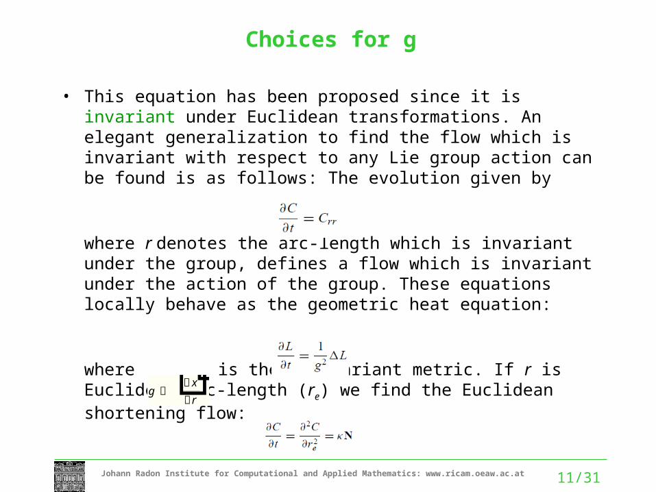
Choices for g

• This equation has been proposed since it is invariant under Euclidean transformations. An elegant generalization to find the flow which is invariant with respect to any Lie group action can be found is as follows: The evolution given by

where r denotes the arc-length which is invariant under the group, defines a flow which is invariant under the action of the group. These equations locally behave as the geometric heat equation:

where is the G-invariant metric. If r is Euclidean arc-length (re) we find the Euclidean shortening flow:

g xr


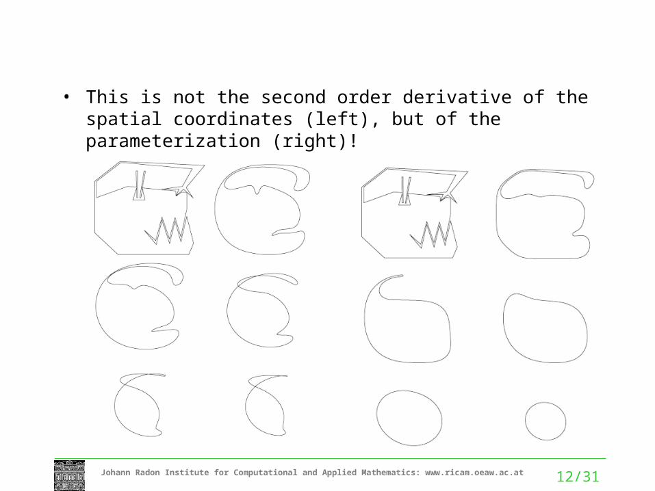
• This is not the second order derivative of the spatial coordinates (left), but of the parameterization (right)!


Choices for g

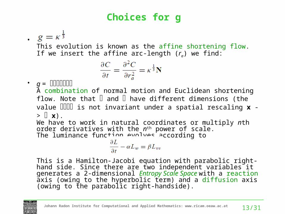
•This evolution is known as the affine shortening flow. If we insert the affine arc-length (ra) we find:

• g = A combination of normal motion and Euclidean shortening flow. Note that and have different dimensions (the value is not invariant under a spatial rescaling x -> x). We have to work in natural coordinates or multiply nth order derivatives with the nth power of scale. The luminance function evolves according to

This is a Hamilton-Jacobi equation with parabolic right-hand side. Since there are two independent variables it generates a 2-dimensional Entropy Scale Space with a reaction axis (owing to the hyperbolic term) and a diffusion axis (owing to the parabolic right-handside).


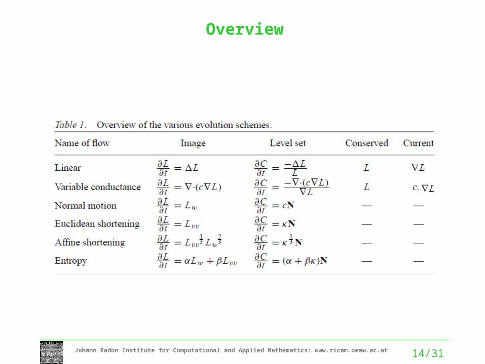
Overview


Numerical stability

• When we approximate a partial differential equation with finite differences in the forward Euler scheme, we want to make large steps in evolution time (or scale) to reach the final evolution in the fastest way, with as little iterations as possible.

• How large steps are we allowed to make? In other words, can we find a criterion for which the equation remains stable?

• A famous answer to the question of stability was derived by Von Neumann, and is called the Von Neumann stability criterion.

• Alternative names:– Courant stability criterion– CFL condition (Courant-Friedrichs-Lewy condition) – …


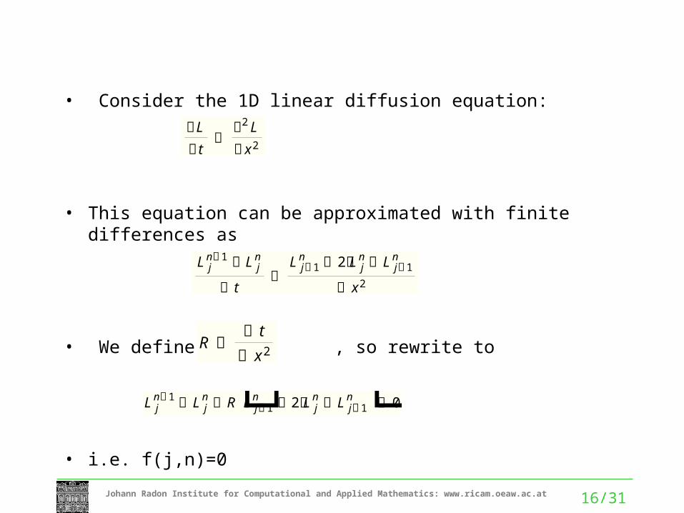
• Consider the 1D linear diffusion equation:

• This equation can be approximated with finite differences as

• We define , so rewrite to

• i.e. f(j,n)=0

Lt

2Lx2

L jn1 L j

n

tL j1n 2L j

n L j1n

x2

R t x2

L jn1 L j

n RL j1n 2L j

n L j1n 0


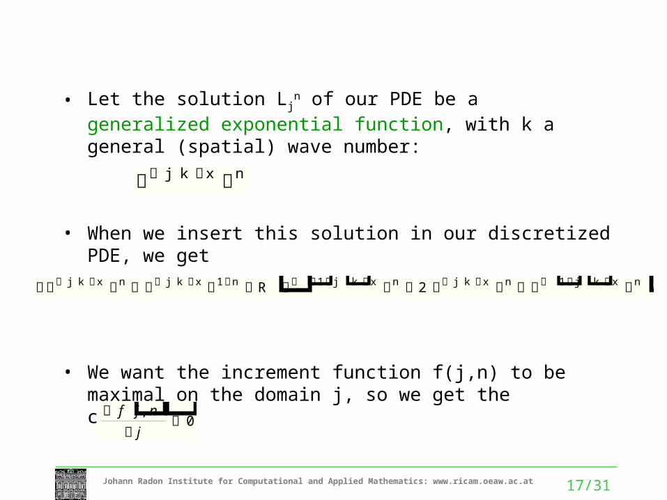
• Let the solution Ljn of our PDE be a generalized

exponential function, with k a general (spatial) wave number:

• When we insert this solution in our discretized PDE, we get

• We want the increment function f(j,n) to be maximal on the domain j, so we get the condition

j k x n

j k x n j k x 1n R1jk x n 2 j k x n 1jk x n fj, n

j 0


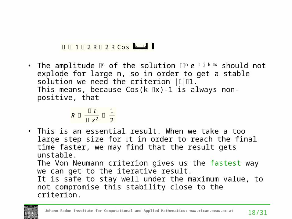
• The amplitude n of the solution n e j k x should not explode for large n, so in order to get a stable solution we need the criterion ||1. This means, because Cos(k x)-1 is always non-positive, that

• This is an essential result. When we take a too large step size for t in order to reach the final time faster, we may find that the result gets unstable. The Von Neumann criterion gives us the fastest way we can get to the iterative result. It is safe to stay well under the maximum value, to not compromise this stability close to the criterion.

R t x2

12

1 2 R 2 R Cosk x


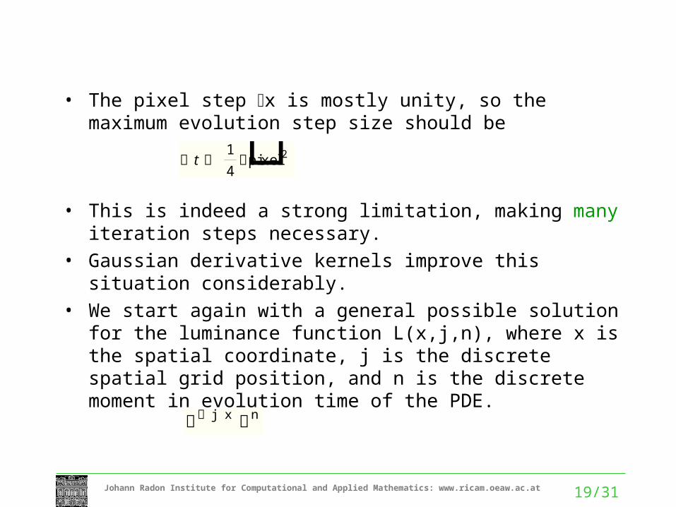
• The pixel step x is mostly unity, so the maximum evolution step size should be

• This is indeed a strong limitation, making many iteration steps necessary.

• Gaussian derivative kernels improve this situation considerably.

• We start again with a general possible solution for the luminance function L(x,j,n), where x is the spatial coordinate, j is the discrete spatial grid position, and n is the discrete moment in evolution time of the PDE.

t 14

pixel2

j x n


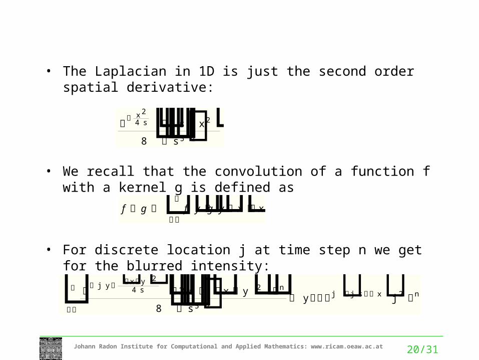
• The Laplacian in 1D is just the second order spatial derivative:

• We recall that the convolution of a function f with a kernel g is defined as

• For discrete location j at time step n we get for the blurred intensity:

x24 s2 s x28 s52

f g

fygy x x

j yxy24 s 2 s x y2n

8 s52 yjj s xj2 n


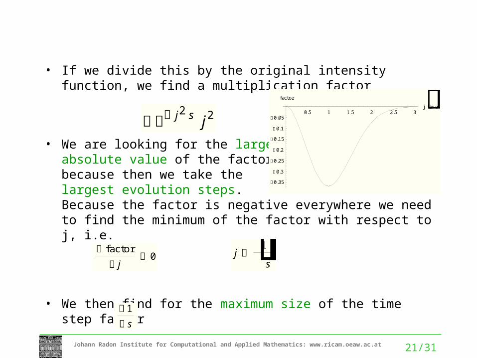
• If we divide this by the original intensity function, we find a multiplication factor

• We are looking for the largest absolute value of the factor, because then we take the largest evolution steps. Because the factor is negative everywhere we need to find the minimum of the factor with respect to j, i.e.

->

• We then find for the maximum size of the time step factor

j2 s j20.5 1 1.5 2 2.5 3

jtime

0.35

0.3

0.25

0.2

0.15

0.1

0.05

factor

factor j

0 j 1s

1s


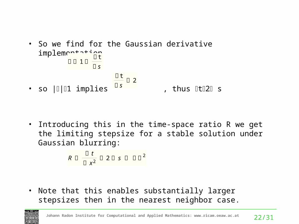
• So we find for the Gaussian derivative implementation

• so ||1 implies , thus t2 s

• Introducing this in the time-space ratio R we get the limiting stepsize for a stable solution under Gaussian blurring:

• Note that this enables substantially larger stepsizes then in the nearest neighbor case.

1 ts

ts

2

R t x2 2 s 2


s 12

2

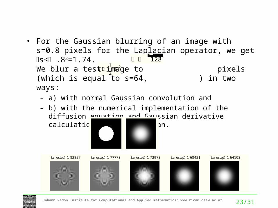
• For the Gaussian blurring of an image with s=0.8 pixels for the Laplacian operator, we get s< .82=1.74. We blur a test image to pixels (which is equal to s=64, ) in two ways: – a) with normal Gaussian convolution and – b) with the numerical implementation of the diffusion

equation and Gaussian derivative calculation of the Laplacian.

128

timestep 1.82857 timestep 1.77778 timestep 1.72973 timestep 1.68421 timestep 1.64103


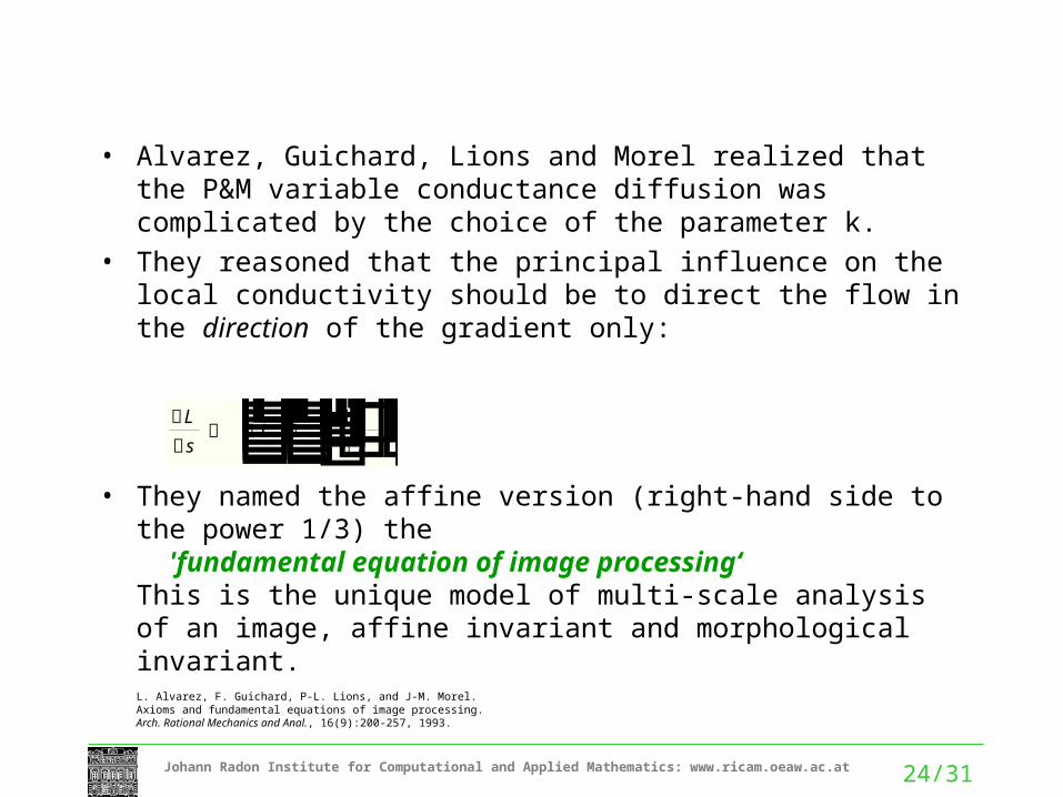
• Alvarez, Guichard, Lions and Morel realized that the P&M variable conductance diffusion was complicated by the choice of the parameter k.

• They reasoned that the principal influence on the local conductivity should be to direct the flow in the direction of the gradient only:

• They named the affine version (right-hand side to the power 1/3) the 'fundamental equation of image processing‘This is the unique model of multi-scale analysis of an image, affine invariant and morphological invariant. L. Alvarez, F. Guichard, P-L. Lions, and J-M. Morel. Axioms and fundamental equations of image processing. Arch. Rational Mechanics and Anal., 16(9):200-257, 1993.

Ls

L.

LL


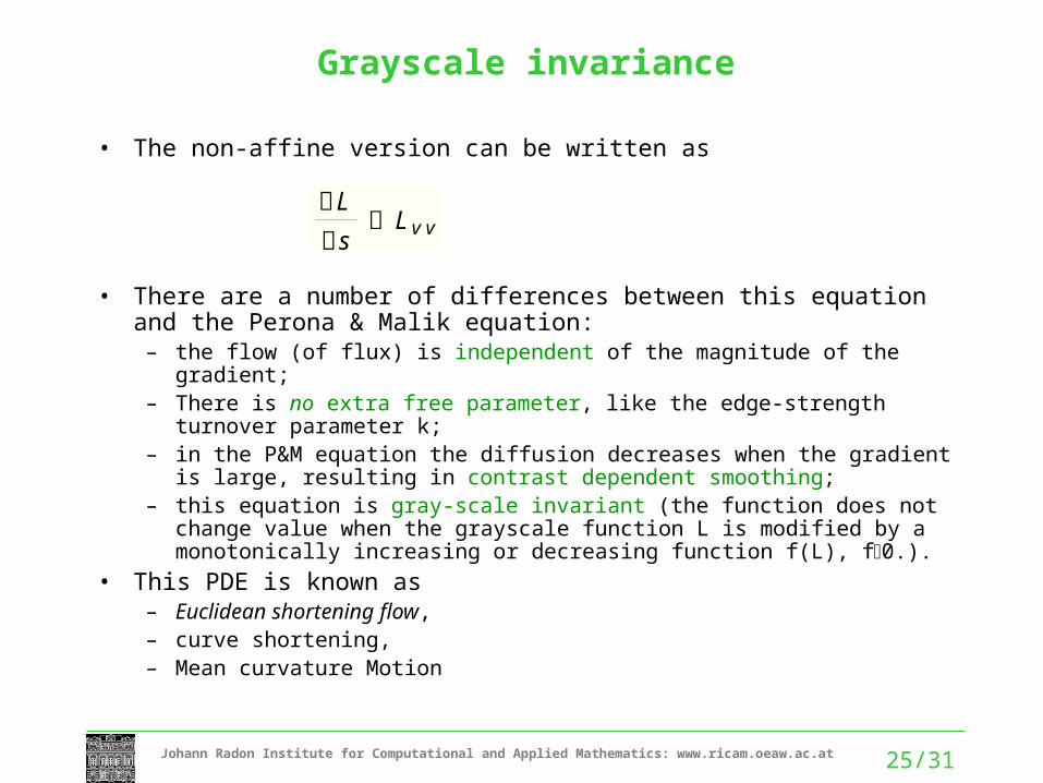
Grayscale invariance

• The non-affine version can be written as

• There are a number of differences between this equation and the Perona & Malik equation: – the flow (of flux) is independent of the magnitude of the gradient; – There is no extra free parameter, like the edge-strength turnover

parameter k; – in the P&M equation the diffusion decreases when the gradient is

large, resulting in contrast dependent smoothing; – this equation is gray-scale invariant (the function does not change

value when the grayscale function L is modified by a monotonically increasing or decreasing function f(L), f0.).

• This PDE is known as – Euclidean shortening flow, – curve shortening, – Mean curvature Motion

Ls

Lv v


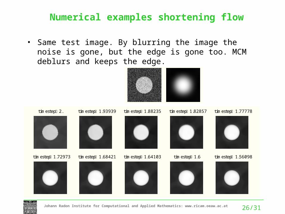
Numerical examples shortening flow

• Same test image. By blurring the image the noise is gone, but the edge is gone too. MCM deblurs and keeps the edge.

timestep 1.72973 timestep 1.68421 timestep 1.64103 timestep 1.6 timestep 1.56098

timestep 2. timestep 1.93939 timestep 1.88235 timestep 1.82857 timestep 1.77778


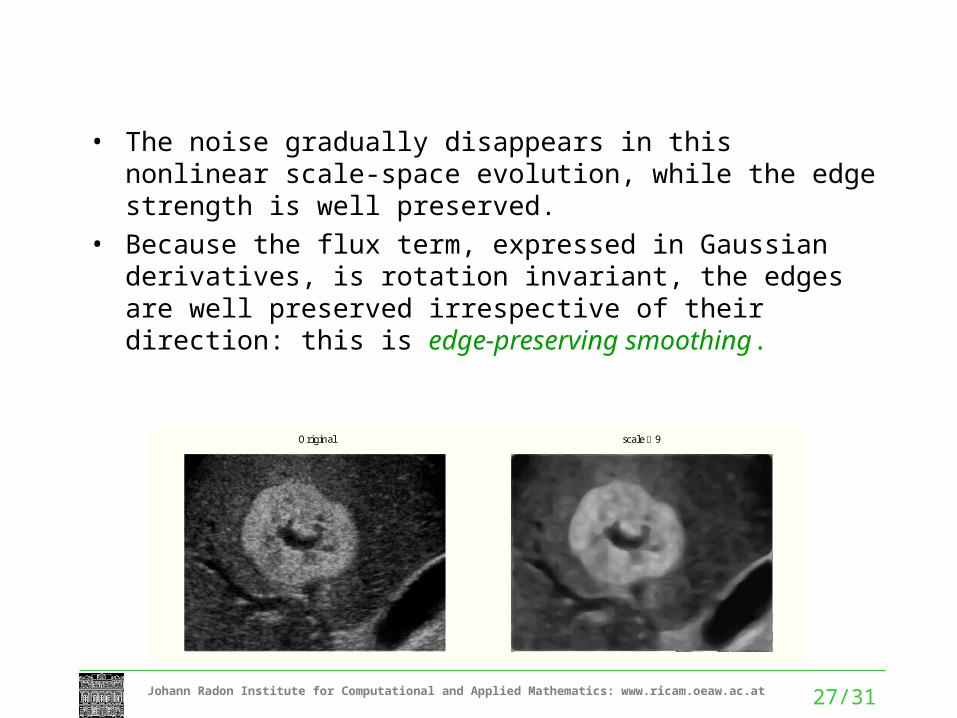
• The noise gradually disappears in this nonlinear scale-space evolution, while the edge strength is well preserved.

• Because the flux term, expressed in Gaussian derivatives, is rotation invariant, the edges are well preserved irrespective of their direction: this is edge-preserving smoothing.

Original scale 9


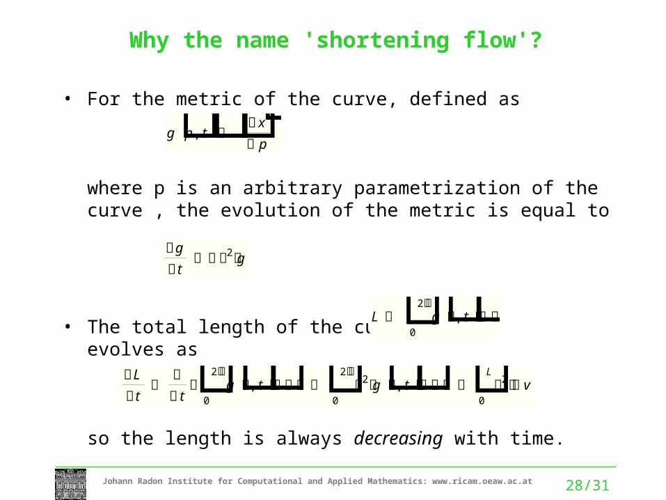
Why the name 'shortening flow'?

• For the metric of the curve, defined as

where p is an arbitrary parametrization of the curve , the evolution of the metric is equal to

• The total length of the curve evolves as

so the length is always decreasing with time.

gt

2g

gp, tx p

L 0

2g, t

Lt

t

0

2g, t

0

22g, t

0

L2v


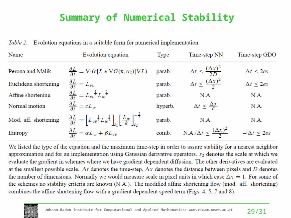
Summary of Numerical Stability


Summary

• There is a strong analogy between curve evolution and PDE based schemes. They can be related directly to one another.

• Euclidean shortening flow involves the diffusion to be limited to the direction perpendicular to the gradient only.

• The divergence of the flow in the equation is equal to the second order gauge derivative Lvv with respect to v, the direction tangential to the isophote.

• Implementation with Gaussian derivatives may allow larger time steps


Next week

• Non-linear diffusion:

Mumford Shah– Diffusion - reaction equations– Energy functional– Edge set

• …

Documents

Signal- und Bildverarbeitung, 323.014 Image Analysis and Processing Arjan Kuijper 30.11.2006