Embed Size (px)
Citation preview

Vom Fachbereich Mathematik der Technischen Universitat Kaiserslautern zur Verleihungdes akademischen Grades Doktor der Naturwissenschaften (Doctor rerum naturalium,Dr. rer. nat.) genehmigte Dissertation
Signature standard bases overprincipal ideal rings
Adrian Popescu
1. Gutachter: Prof. Dr. Gerhard Pfister2. Gutachter: Prof. Dr. Martin Kreuzer
Vollzug der Promotion: 28 September 2016
D 386

Page
Abstract i
Acknowledgments v
Preface vii
A Standard bases over rings 1
1 Buchberger’s Algorithm 3A:1.1 Basic definitions and notations . . . . . . . . . . . . . . . . . . . . . . . 3A:1.2 Buchberger’s algorithm blueprint . . . . . . . . . . . . . . . . . . . . . . 7A:1.3 ALL vs. JUST . . . . . . . . . . . . . . . . . . . . . . . . . . . . . . . . . 12A:1.4 Huge coefficients over the integers . . . . . . . . . . . . . . . . . . . . . 14A:1.5 Strong pairs in the reduction procedure . . . . . . . . . . . . . . . . . . 16
2 Signature standard bases over the integers 21A:2.1 Definitions and notations . . . . . . . . . . . . . . . . . . . . . . . . . . 21A:2.2 Criteria: Syzygy, Rewrite and F5C . . . . . . . . . . . . . . . . . . . . . 25A:2.3 SigDrops . . . . . . . . . . . . . . . . . . . . . . . . . . . . . . . . . . . 35A:2.4 Timings . . . . . . . . . . . . . . . . . . . . . . . . . . . . . . . . . . . . 40A:2.5 Finite rings − Zm . . . . . . . . . . . . . . . . . . . . . . . . . . . . . . . 41
B Depth, Stanley Depth and Hilbert Depth 45
1 Definitions and Notations 49B:1.1 Cohen−Macaulay Modules . . . . . . . . . . . . . . . . . . . . . . . . . 49B:1.2 Hilbert Function and Hilbert Polynomial . . . . . . . . . . . . . . . . . . 50
2 Hilbert Depth 55B:2.1 Hilbert Series and Hilbert Depth . . . . . . . . . . . . . . . . . . . . . . 55B:2.2 Computational Experiments . . . . . . . . . . . . . . . . . . . . . . . . . 60B:2.3 The hdepth procedure . . . . . . . . . . . . . . . . . . . . . . . . . . . . 62
3 The Stanley Conjecture 63B:3.1 The present stay of Stanley’s Conjecture and its impact in Commutative
Algebra . . . . . . . . . . . . . . . . . . . . . . . . . . . . . . . . . . . . 63B:3.2 The Stanley Conjecture on intersections of three monomial prime ideals. 65B:3.3 The Stanley Conjecture for factors of monomial ideals . . . . . . . . . . 74B:3.4 A special case of r = 4 . . . . . . . . . . . . . . . . . . . . . . . . . . . . 77
B:3.5 Proof of Theorem B:3.3.7 . . . . . . . . . . . . . . . . . . . . . . . . . . 78
4 Stanley depth of factors of monomial ideals 85B:4.1 The canonical form of a factor of monomial ideals . . . . . . . . . . . . 86B:4.2 The canonical form algorithm . . . . . . . . . . . . . . . . . . . . . . . . 91
C Constructive General Neron Desingularization 95
1 Artin approximation and General Neron Desingularization 99
2 A method to compute a General Neron Desingularization in the frame ofone dimensional local domains 103
3 The implementation in SINGULAR and some examples 115
Appendix 127
Examples used in Part A 129Examples for ALL vs JUST strategies . . . . . . . . . . . . . . . . . . . . . . . 131Example 18 . . . . . . . . . . . . . . . . . . . . . . . . . . . . . . . . . . . . . 133Examples for Signature Algorithm . . . . . . . . . . . . . . . . . . . . . . . . . 137
Programming in SINGULAR ’s kernel 141Introduction . . . . . . . . . . . . . . . . . . . . . . . . . . . . . . . . . . . . . 143Git, Compilation and Building . . . . . . . . . . . . . . . . . . . . . . . . . . . 145Internal structures . . . . . . . . . . . . . . . . . . . . . . . . . . . . . . . . . 149Searching functions from the interpreter . . . . . . . . . . . . . . . . . . . . . 157Adding new features . . . . . . . . . . . . . . . . . . . . . . . . . . . . . . . . 161
ABSTRACT
By using Grobner bases of ideals of polynomial algebras over a field, many imple-mented algorithms manage to give exciting examples and counter examples in Com-mutative Algebra and Algebraic Geometry. Part A of this thesis will focus on extendingthe concept of Grobner bases and Standard bases for polynomial algebras over the ringof integers and its factors Zm[x]. Moreover we implemented two algorithms for thiscase in SINGULAR which use different approaches in detecting useless computations,the classical Buchberger algorithm and a F5 signature based algorithm.
Part B includes two algorithms that compute the graded Hilbert depth of a gradedmodule over a polynomial algebra R over a field, as well as the depth and the multi-graded Stanley depth of a factor of monomial ideals of R. The two algorithms providefaster computations and examples that lead B. Ichim and A. Zarojanu to a counter ex-ample of a question of J. Herzog. A. Duval, B. Goeckner, C. Klivans and J. Martin haverecently discovered a counter example for the Stanley Conjecture. We prove in thisthesis that the Stanley Conjecture holds in some special cases.
Part C explores the General Neron Desingularization in the frame of Noetherianlocal domains of dimension 1. We have constructed and implemented in SINGULAR andalgorithm that computes a strong Artin Approximation for Cohen−Macaulay local ringsof dimension 1.
Technische Universitat Kaiserslautern i

Fur Polynomringe uber Korpern sind Grobnerbasen ein wichtiges Hilfsmittel furBerechnungen in der kommutativen Algebra und der algebraischen Geometrie. Teil Adieser Dissertation behandelt die Verallgemeinerung des Konzepts der Grobnerbasis undStandardbasis fur Polynomringen uber dem Ring der ganzen Zahlen und seinen Faktor-ringen. Hierbei haben wir theoretische Aspekte untersucht und eine Vielzahl neuerStrategien entwickelt. Darauf aufbauend haben wir zwei verschiedene Algorithmen imComputeralgebrasystem SINGULAR implementiert, die sich durch ihre Kriterien zumFinden unnotiger Berechnungen grundlegend unterscheiden, den Buchberger Algorith-mus und den signaturbasierte F5 Algorithmus.
Der Teil B beinhaltet zwei Algorithmen zum Berechnen der graduierten Hilberttiefevon graduierten Moduln uber einer polynomialen Algebra R uber einem Korper, sowieder Tiefe und der multigraduierten Stanleytiefe eines Faktors eines monomialen Ide-als von R. Die beiden Algorithmen bieten schnellere Berechnungsverfahren, die zuBeispielen gefuhrt haben, die B. Ichim und A. Zarojanu nutzen konnten ein Gegen-beispiel fur eine Frage von J. Herzog zu finden. Vor Kurzem erst haben A. Duval, B.Goeckner, C. Klivans und J. Martin ein Gegenbeispiel zur Stanley Vermutung gefunden.Wir zeigen in dieser Arbeit, dass die Stanley Vermutung in speziellen Fallen richtig ist.
Der Teil C ist der allgemeinen Neron Desingularisierung im Fall von Noetherschen,lokalen Bereichen der Dimension 1 gewidmet. Hier wurde ein Algorithmus zur Berech-nung der Artinsche Approximation fur lokale Cohen−Macaulay Ringe der Dimension 1entwickelt.
Technische Universitat Kaiserslautern iii


ACKNOWLEDGMENTS
I would like to thank Gerhard Pfister for being much more than a professor;Christian Eder for always having time for my standard bases questions and for workingon them together; Hans Schonemann for been able to answer all my SINGULAR -relatedquestions; Wolfram Decker and Christoph Lossen for finding financial support withoutwhich this thesis would not have been possible; Anne Fruhbis-Kruger for the help in de-veloping new strategies used in solving integer related bugs, Jakob Kroker for sendingmany bugs regarding the standard bases over rings and to Petra Basell for helping mein any other problem.
I would also like to thank Natalie for spending lots of time correcting my Englishmistakes and special thanks to my parents, Adriana and Dorin, who supported andmotivated me.
Danke :)
Technische Universitat Kaiserslautern v

PREFACE
This thesis is structured into three parts that approach different branches inComputer Algebra and Commutative Algebra and Programming in SINGULAR ’s sources.The preface will provide the reader a brief history of the main concepts used in each ofthese parts and an overall description of this papers structure.
PART A − Standard Bases over Rings
The notion of Grobner bases was first introduced in 1965 by Buchberger in his PhDthesis [Bu]. Independently, Grauert and Hironaka introduced the notion of standardbases, a generalization of the Grobner bases. This concept proves to be useful in a widerange of fields like Commutative Algebra, Singularity Theory and Algebraic Geometry.They are used in solving system of polynomial equations, ideal intersection problemsand even resolving Sudoku puzzles. The standard bases serve as a stepping stone ofa relatively new mathematical field: Computer Algebra. Although the main idea ofBuchberger’s algorithm still remains the same, many new strategies and criteria weredeveloped to speed up the algorithm.
O. Wienand has modified the Grobner basis algorithm to work well over base ringsthat are not necessarily fields and may have zero divisors. The author has extendedWienand’s implementation of the algorithm in SINGULAR also for local and mixed or-derings in his Master thesis. Here we review the algorithm and add some strategies tospeed up the computations, especially when working over the integers.
In 2002 Faugere introduced the F5 algorithm. A lot of the computations in Buch-berger’s algorithm give no new information for the standard basis. The F5 algorithmprovides strategies to detect and eliminate some of these useless computations by usingsignatures. A very interesting survey on the F5 algorithms and variants can be foundin [EF]. C. Eder studied and implemented a variant of F5 in SINGULAR . This paperprovides a generalization of this algorithm over rings that are not necessarily fields.
PART B − Depth, Stanley Depth and Hilbert Depth
In 1982, Richard Stanley has conjectured an upper bound for the depth of a multi-graded module (see [St]). Nowadays this is known as the Stanley Conjecture and itsurprisingly connects two notions: depth − a homological invariant and the Stanleydepth − a combinatorial concept defined by Stanley Decompositions. At a first glanceno connection between these can be established, but after a closer look similarities can
Technische Universitat Kaiserslautern vii
be established: if the Stanley depth is 0, then the depth is 0. Rinaldo published analgorithm that computes the Stanley depth of a quotient of monomial ideals and im-plemented it in [CoCoA]. After the introduction of the canonical form we were able tospeed up this algorithm (see [AP2]).
The conjecture has been open for more than 30 years and in the last 10 years manypapers prove particular cases of it. However, in 2016 a counterexample was publishedin [DuGo]. A survey concerning the Stanley depth has been published by J. Herzog;before this counterexample was found and contains an overview of most of the knownresults up to 2011 (see [H]).
Stanley decompositions prove to be very useful in describing finitely generatedgraded algebras, e.g. rings of invariants under some group action (see Sturmfels andWhite [SW]), and in applications of the normal form theory for systems of differentialequations with nilpotent linear part (see Murdock and Sanders [MS]). Another aston-ishing result concerning the Stanley conjecture is the following result from [HSY] stat-ing that if the conjecture holds for the Stanley-Reisner of a certain simplicial complexthen it is partitionable.
Herzog, Vladoiu and Zheng proved in [HVZ] that the module structure is alreadygiven by the Hilbert series and therefore the Stanley depth may be computed from this.Based on this idea, Bruns, Krattenthaler and Uliczka introduced in [BKU] the Hilbertdepth − a similar notion to the Stanley depth. We introduce a first algorithm thatcomputes the Hilbert depth and implemented it in SINGULAR .
PART C − Constructive General Neron Desingularization
The Implicit Mapping Theorem plays an important role in Singularity Theory andAnalytic Geometry. A Noetherian local ring (R,m) has the Artin Approximation Propertyif each finite system of polynomials equations over R has a solution in R iff it has a solutionin the completion R. This can be formulated as follows: for every c ∈ N, each solution ofthis system y from R can be approximated with a solution y in R modulo mc. M. Artinproved in 1969 that the algebraic power series over a field has the Artin ApproximationProperty (see [Artin1]). In 1986, D. Popescu proved that each excellent Henselian localring has this property (see [DP2]) by using the existence of a so-called General NeronDesingularization. D. Popescu and the author gave an algorithmic proof of the existenceof a General Neron Desingularization in the frame of one dimensional local domains(see [APDP2]) and implemented this algorithm in SINGULAR . A generalization of thisalgorithm was later published by G. Pfister and D. Popescu (see [PfPo2]).
Many applications of the Artin Approximation Property in Singularity theory andCommutative Algebra have been presented in a series of conferences hosted in Luminy,Marseilles, France organized by H. Hauser and G. Rond at the beginning of 2015.
viii Adrian Popescu
THE STRUCTURE
In Chapter A:1 we introduce the reader to a series of basic definitions and notationsfrom the standard bases theory together with the classic Buchberger Algorithm to com-pute a Grobner basis. We continue by expanding the above mentioned concepts to thecase when the ground ring is a principal ideal ring that is not a field (as an extensionof O. Wienands PhD Thesis [W]). This chapter also provides a description of severalstrategies that will decrease the run time and memory of the algorithm.
Chapter A:2 consists of Faugere’s F5 algorithm, optimized and implemented inSINGULAR by C. Eder over fields, and a generalization of the strategy for principalideal rings. We also describe the difficulties that arise on this approach together witha couple of ideas that will overcome these obstacles. At the very end we compare theBuchberger Algorithm with this version of F5 over the ring of integers on some randomexamples.
Chapter B:1 introduces the basic definitions and notations used throughout Part Band explores in details concepts like the depth of a module, Hilbert Series and Stanleyand Hilbert decomposition.
Chapter B:2 consists of a procedure that computes the Hilbert depth of a mod-ule. This is the first in a line of algorithms that recently appeared in order to computehdepth. This chapter was published in the Journal of Symbolic Computation [AP2].
In Chapter B:3 we take an in depth look of the Stanley Conjecture. After a shortintroduction of the conjecture, we present some new results in which the conjectureholds. This chapter was partially published in several papers (see [AP1], [AP3] and[APDP1]).
Chapter B:4 introduces the new notion of canonical form that is later used to op-timize Rinaldo’s algorithm for the Stanley depth computation. This chapter was pub-lished in Bulletin Mathematique de la Societe des Sciences Mathematiques de Roumanie([AP3]).
Part C starts with a small introduction on Artin Approximation and the GeneralNeron Desingularization. It also contains an algorithmic proof in the case of Noethe-rian local domains of dimension 1. The algorithm for this case was implemented inSINGULAR . This part has also been published (see [APDP2]).
At the very end the Appendix contains several important examples used throughoutthe thesis together with a part exploring the source code of SINGULAR on page 143.
Technische Universitat Kaiserslautern ix

PART A
STANDARD BASES OVER RINGS
Technische Universitat Kaiserslautern 1

CHAPTER A:1
BUCHBERGER’S ALGORITHM
In this chapter we introduce the basic notions for standard bases and the additionalstrategies needed when the polynomial algebra is defined over a ring that is not neces-sarily a field.
A:1.1 Basic definitions and notations
DEFINITION A:1.1.1.Let Mon(x1, . . . , xn) be the set of monomials in n ∈ N variables x1, . . . , xn. We denote
by x the set of all variables and for α = (α1, . . . , αn) ∈ Nn we set xα := xα11 · . . . · xαnn .
A monomial ordering < is a total ordering on Mon(x) satisfying the following prop-erty
xα < xβ =⇒ xγ · xα < xγ · xβ for all α, β, γ ∈ Nn.
A monomial ordering is called global if 1 = x0 ≤ xα for all α ∈ Nn.A monomial ordering is called local if 1 = x0 ≥ xα for all α ∈ Nn.A monomial ordering is called mixed if there is α, β ∈ Nn such that xα < 1 < xβ.
DEFINITION A:1.1.2.Let < be a monomial ordering on Mon(x), R be a ring and f ∈ R[x] := R[x1, . . . , xn]
a polynomial. We can write f in a unique way
f =L∑i=1
ci · xα(i)
,
0 6= ci ∈ R and α(i) ∈ Nn for 1 ≤ i ≤ L such that xα(1)< . . . < xα
(L). We define
◦ the length of f denoted by `(f) = L,
◦ the leading term denoted by LT(f) = cL · xα(L),
◦ the leading coefficient denoted by LC(f) = cL,
◦ the leading monomial denoted by LM(f) = xα(L),
◦ the tail of f denoted by tail(f) = f − LT(f),
Technische Universitat Kaiserslautern 3
◦ the degree of f denoted by deg(f) = max1≤i≤L
{α(i)1 + . . .+ α(i)
n
}and
◦ the ecart of f denoted by ecart(f) = deg(f)− deg(
LT(f)).
In the following we define some common monomial orderings and provide a smallexample to see the differences between them.
DEFINITION A:1.1.3.
◦ negative degree reverse lexicographical ordering (called ds in SINGULAR ). Thislocal ordering is defined on R[x] as follows:
xα <ds xβ ⇐⇒
n∑i=1
αi =: deg(xα) > deg(xβ) or
deg(xα) = deg(xβ) and ∃1 ≤ i ≤ n s.t. αn = βn, . . . , αi+1 = βi+1, αi > βi.(A:1.1)
◦ negative lexicographical ordering (called ls in SINGULAR ). This local orderingis defined on R[x] as follows:
xα <ls xβ ⇐⇒ ∃ 1 ≤ i ≤ n s.t. α1 = β1, . . . , αi−1 = βi−1, αi > βi. (A:1.2)
◦ degree reverse lexicographical ordering (called dp in SINGULAR ). This globalordering is defined on R[x] as follows:
xα <dp xβ ⇐⇒
n∑i=1
αi =: deg(xα) < deg(xβ) or
deg(xα) = deg(xβ) and ∃1 ≤ i ≤ n s.t. αn = βn, . . . , αi+1 = βi+1, αi < βi.(A:1.3)
◦ lexicographical ordering (called lp in SINGULAR ). This global ordering is definedon R[x] as follows:
xα <lp xβ ⇐⇒ ∃ 1 ≤ i ≤ n s.t. α1 = β1, . . . , αi−1 = βi−1, αi < βi. (A:1.4)
◦ weighted orderings. All the above degree orderings can be enhanced by introduc-ing weights. For a vector w =
(w1, . . . , wn
)∈ Zn we define the weighted degree of
xα byw-deg(xα) = w1α1 + . . .+ wnαn.
4 Adrian Popescu
We define the weighted reverse lexicographic ordering, denoted by wp(w1, . . . , wn),by replacing deg by w-deg in the Equation A:1.3.
Similarly we define the weighted negative reverse lexicographic ordering, de-noted by ws(w1, . . . , wn), by changing Equation A:1.1.
EXAMPLE A:1.1.4. Consider f = xyz + x2 + z2 + y ∈ R[x, y, z]. Below we write f in itsunique form for each of the monomial orderings from Definition A:1.1.3.
<dp: xyz + x2 + z2 + y
<lp: x2 + xyz + y + z2
<ls: z2 + y + xyz + x2
<ds: y + x2 + z2 + xyz
We notice that in this example, each of the 4 monomials can be seen as the leading termdepending on the monomial ordering.
REMARK A:1.1.5. Unfortunately, this is not true in general. Consider f = x2 +xy+ y2 ∈R[x, y]. There is no monomial ordering such that xy is the leading monomial of f .
Proof.Let < be a monomial ordering. There are two cases:
◦ x < y. In this case multiplying by x, respectively y gives us that LT(f) = y2.
◦ x > y. Similarly, LT(f) = x2.
DEFINITION A:1.1.6.Let I ⊆ R[x] be an ideal.The leading ideal of I is L<(I) = 〈{LT(f) | f ∈ I}〉.The leading monomial ideal of I is LM<(I) = 〈{LM(f) | f ∈ I}〉.The leading ideal for a set of polynomials S := {f1, . . . , fm} is defined to be the
leading ideal of the ideal generated by S.From now on, if the monomial ordering is clear from the context, we will only write
L(I) (respectively LM(I)) instead of L<(I) (respectively LM<(I)).
REMARK A:1.1.7. When R is a field it is easy to see that L<(I) = LM<(I) for any idealI ⊂ R[x]. This is not true overR[x] ifR is a ring that is not a field. For instance over Z[x],L<(〈2x〉
)= 〈2x〉 ( 〈x〉 = LM<
(〈2x〉
). In general L<(I) ⊆ LM<(I), but the converse
does not always hold for rings that are no fields, as shown in the example above. Asone would expect, the leading coefficients play an important role.
Throughout Part A when speaking about rings, we will refer in fact to rings that areno fields.
Technische Universitat Kaiserslautern 5
DEFINITION A:1.1.8 (Standard Bases).A standard basis of an ideal I ⊂ R[x] with respect to a fixed monomial ordering <
is a finite set S ⊂ I such that L(I) = L(S).S is a strong standard basis if additionally it satisfies the following property:
∀f ∈ I,∃ g ∈ S such that LT(g) | LT(f).
REMARK A:1.1.9. Note that in the case of fields all standard bases S are strong sincewe can always set the leading coefficient of a polynomial g ∈ S to be 1 by multiplying gwith its inverse LC(g)−1. Over rings this is not true, as shown in the following example.
EXAMPLE A:1.1.10. Consider the ideal I = 〈4x, 13x〉 = 〈x〉 over Z[x]. It is easy to seethat S = {4x, 13x} is a standard basis for I. Take f = 2x ∈ I and since 4x nor 13xdivides f , S is not a strong standard basis of I. A strong standard basis for I is S ′ = {x}.
DEFINITION A:1.1.11.A ring R is a principal ideal ring if each ideal I of R can be generated using a single
element.
DEFINITION A:1.1.12.Let I ⊂ R be an ideal. The annihilator (or annulator) of I, denoted by Ann(I), is
Ann(I) = {c ∈ R | c ·m = 0,∀m ∈ I} .
For an element c ∈ R, we will shortly denote by Ann(c) = Ann(〈c〉).
We extend the previous definitions and notations over modules. Let I = 〈f1, . . . , fs〉
an ideal in R[x] and R[x]s be the free R[x] modules⊕i=1
R[x] · εi, where εi is the canonical
basis.
DEFINITION A:1.1.13.A monomial in the module case is an element of the formm·εi =
(0, . . . , 0,m, 0, . . . , 0
)∈ R[x]s where m is a monomial in R[x] and it is located on the i−th component whileall the others components are 0.
DEFINITION A:1.1.14.A module monomial ordering (or simply called module ordering) is a total order-
ing ≺ on the set of monomials of R[x]s compatible with the monomial ordering < onR[x], i.e.
◦ mα < mβ =⇒ mα · εi ≺ mβ · εi,
◦ mα · εi ≺ mβ · εj =⇒ mαmγ · εi ≺ mβmγ · εj,
6 Adrian Popescu
for all monomials mα, mβ, mγ in R[x] and for each i, j = 1, . . . , s.
Definition A:1.1.2 simply extends to the module case.There are 4 canonical ways to naturally extend the ring ordering < to a module
ordering by regarding the components as shown in the example below.
EXAMPLE A:1.1.15 (Module orderings). We define the following module orderings:
◦ ≺(c,<)
mα · εi ≺(c,<) mβ · εj ⇐⇒ i > j ori = j and mα < mβ.
◦ ≺(C,<)
mα · εi ≺(C,<) mβ · εj ⇐⇒ i < j ori = j and mα < mβ.
◦ ≺(<,c)
mα · εi ≺(<,c) mβ · εj ⇐⇒ mα < mβ ormα = mβ and i > j.
◦ ≺(<,C)
mα · εi ≺(<,C) mβ · εj ⇐⇒ mα < mβ ormα = mβ and i < j.
DEFINITION A:1.1.16 (syzygy).Let I = 〈f1, . . . , fs〉 be an ideal in R[x]. Consider the map
π :s⊕i=1
R[x] · εi // R[x]
εi� // fi
A syzygy is an element s ∈ kerπ.
A:1.2 Buchberger’s algorithm blueprint
This section presents a simple Buchberger algorithm blueprint for computing stan-dard bases in polynomial rings over principal ideal rings. For this we introduce somemore basic notions.
In the following, let R be a ring. Usually we will take R to be Z or Zr := Z/rZ wherer ∈ Z is not a prime number. Let f, g ∈ R[x] be two polynomials such that
f = cf ·mf + . . .
Technische Universitat Kaiserslautern 7
g = cg ·mg + . . .
with LT(f) = cf ·mf and LT(g) = cg ·mg.
DEFINITION A:1.2.1.We define several important polynomials used in the strong standard bases theory.
◦ The s−polynomial (or s−pair) of f and g, denoted by
s-poly(f, g) =lcm(cf , cg) lcm (mf ,mg)
cfmf
· f − lcm(cf , cg) lcm (mf ,mg)
cgmg
· g.
Note that the leading terms will cancel out.
◦ Since R is a principal ideal ring, we have that 〈cf , cg〉 = 〈c〉. Let c = df · cf + dg · cg.The strong polynomial (or the gcd polynomial, gcd−pair, strong pair) of f andg denoted by
gcd-poly(f, g) =df lcm(mf ,mg)
mf
· f +dg lcm(mf ,mg)
mg
· g.
Notice that LT(
gcd-poly(f, g))
= c · lcm(mf ,mg).
◦ In case of rings with zero divisors, the extended s−polynomial of f denoted by
ext-poly(f) = Ann(cf ) · f = Ann(cf ) · tail(f).
Note that if LC(f) is not a zero divisor then ext-poly(f) = 0.
REMARK A:1.2.2. Note that in the definition of gcd−pairs df and dg are not uniquelydetermined. For instance, 〈3, 5〉 = 〈1〉 and we can consider several df and dg:
2 · 3 + (−1) · 5 = 1(−3) · 3 + 2 · 5 = 1
7 · 3 + (−4) · 5 = 1
However, it is easy to prove that we can randomly choose one of them, since theywill give dependent polynomials with respect to the s−polynomial. For this, see thenext lemma.
LEMMA A:1.2.3.Let two polynomials f, g ∈ R[x],
f = cf ·mf + . . . ,
g = cg ·mg + . . . ,
such that 〈c〉 = 〈cf , cg〉. Let df 6= d′f , dg 6= d′g such that
df · cf + dg · cg = c = d′f · cF + d′g · cg.
Denote by P and Q the gcd−polynomial constructed with df ,dg, respectively d′f and d′g.Then P = Q+ α · s-poly(f, g) for an α ∈ R.
8 Adrian Popescu
Proof.By definition,
s-poly(f, g) =L
cf· lcm(mf ,mg)
mf
· f − L
cg· lcm(mf ,mg)
mg
· g,
where L = lcm(cf , cg),
P = df ·lcm(mf ,mg)
mf
· f + dg ·lcm(mf ,mg)
mg
· g,
and
Q = d′f ·lcm(mf ,mg)
mf
· f + d′g ·lcm(mf ,mg)
mg
· g.
One can easily see that
P −Q = (df − d′f ) ·lcm(mf ,mg)
mf
· f + (dg − d′g) ·lcm(mf ,mg)
mg
· g.
Using the choice of df , d′f , dg and d′g, we know that
(df − d′f ) · cf = −(dg − d′g) · cg,
and thereforedf − d′fL
cf
= −dg − d′gL
cg
=: α.
This is the α we needed and hence we are done.
EXAMPLE A:1.2.4. Consider two polynomials f = 5x3 + 5xy + 3y and g = 3y2 + 2x inZ10[x, y] and the dp (degree reverse lexicographical) ordering. Then
◦ s-poly(f, g) = 3y2 · f − 5x3 · g = 5xy3 + 9y3,
◦ gcd-poly(f, g) = −y2 · f + 2x3 · g = x3y2 + 4x4 + 5xy3 + 7y3,
◦ ext-poly(f) = 2 · f = 6y and
◦ ext-poly(g) = 0 · g = 0.
REMARK A:1.2.5. Note that if 〈cf , cg〉 = 〈cf〉, then we can take df = 1 and dg = 0.
Therefore gcd-poly (f, g) = m · f , for the monomial m =lcm(mf ,mg)
mf
. In other words if
one of the leading coefficients divides the other, then the gcd-poly is equal to a multipleof the initial polynomial and, as we will later see, it brings no new information. We callsuch a gcd−polynomial redundant.
Technische Universitat Kaiserslautern 9
DEFINITION A:1.2.6.Let S = {f ∈ R[x] | LM(f) = 1 and LC(f) is a unit in R}. Denote by
R[x]< := S−1R[x].
Note that if < is a global ordering, R[x]< = R[x] and when < is a local or mixedordering, R[x]< = R[x]〈x〉.
DEFINITION A:1.2.7.Let G be the set of all finite subsets G ⊂ R[x]<. The map
NF : R[x]< × G // R[x]
(f,G) � // NF(f | G)
is called a weak normal form if for each f ∈ R[x]< and each finite set of polynomialsG ⊂ R[x]<, the following properties hold:
◦ NF(0 | G) = 0,
◦ if NF(f | G) 6= 0, then LT(
NF(f | G))6∈ L(G) and
◦ for f 6= 0, there exists a unit u ∈ R[x]< such that either u · f = NF(f | G) or theremainder r = u · f − NF(f | G) has a standard representation w.r.t. G, that is
r =∑g∈G
cg · g, where cg ∈ R,
LM(r) ≥ LM(cg) · LM(g) for all g s.t. cg · g 6= 0.
A weak normal form is simply called a normal form if one can always choose u = 1in the standard representation.
An algorithm to compute the weak normal form over fields can be found in theSINGULAR book [GP, Algorithm 1.7.6]. The algorithm will look as below, if the mono-mial ordering is global.
Algorithm reduce(poly f, ideal G)Input: f ∈ R[x] and a finite subset G ⊂ R[x] on which we consider a global orderingOutput: h ∈ R[x], a weak normal form of f w.r.t. G
1: h = f ;2: while exists g ∈ G s.t. LT(g) | LT(h) do3: h = s-poly(h, g);4: return h
Note that on line 3 of the algorithm, with each s-poly computation, the leadingmonomial of h will decrease. This algorithm only works for global orderings. If the
10 Adrian Popescu
orderings are local or mixed, we need to also consider the ecart of h. This is explainedin Section A:1.5.
The normal form plays an important role in the standard basis computation becauseof Buchberger’s Criterion described below.
LEMMA A:1.2.8(Buchberger Criterion,[GP, Theorem 1.7.3]
).
Let I and ideal in R[x] and a set G = {g1, . . . , gs} ⊂ I. Let NF(·|G) be a weak normalform on R[x] with respect to G. Then the following are equivalent:
1. G is a standard basis of I
2. NF(f | G) = 0 for all f ∈ I
3. each f ∈ I has a standard representation with respect to G
4. G generates I and NF(
s-poly(gi, gj) | G)
= 0 for 1 ≤ i, j ≤ s.
REMARK A:1.2.9. Note that the elements of a standard basis generate not just the lead-ing ideal but the ideal itself. Therefore, one can view the standard bases as a set ofgenerators of an ideal with special properties.
We are now ready to show the algorithm’s blueprint.
ALGORITHM A:1.2.10 (Buchberger’s blueprint).LetR be a principal ideal ring,< a monomial ordering onR[x] and I = 〈f1, . . . , fr〉 ⊂
R[x] be an ideal. The following algorithm returns a strong standard basis S = {g1, . . . , gt}of I.
1: S = {f1, . . . , fr};2: L = {s-poly(fi, fj) | i < j} ∪ {gcd-poly(fi, fj) | i < j} ∪ {ext-poly(fi)};3: while L 6= ∅ do4: choose h ∈ L and reduce it with S;5: if h 6= 0 then6: S = S ∪ {h};7: L = L ∪ {s-poly(g, h) | g ∈ S} ∪ {gcd-poly(g, h) | g ∈ S} ∪ {ext-poly(h)};8: return S
The set L will be called the pair list. Through the reduction on line 4 we understandcomputing a normal form as in the algorithm described earlier.
REMARK A:1.2.11. When working with a polynomial ring over a field, we just add of thes−polynomials in line 7 of the algorithm. If R is a ring, the following natural questionsarise:
Technische Universitat Kaiserslautern 11
Why do we need extended s−polynomials?
Let I = 〈f〉 ⊂ Z10[x, y] be an ideal, where f = 5x3 + 5xy + 3y and consider the dp
ordering. Algorithm A:1.2.10 without adding the extended s-polynomial yields S = {f}as a strong standard basis with L(S) = 〈5x3〉. But since I is an ideal and f ∈ I, then2f ∈ I implying LT(2f) = 6y ∈ L(I) = L(S). Therefore, S should also contain 2f , andhence the extended s−polynomial of f , ext-poly(f). This is the reason why we need toadd ext-poly(f) in the case of zero divisors.
Why do we need strong / gcd polynomials?
Example A:1.1.10 gives us a quick answer. If we compute the strong standard basiswith Algorithm A:1.2.10 without considering the strong pairs, then we would get S =〈4x, 13x〉 as a strong standard basis, which is false. If we add gcd-poly (4x, 13x) = x toS, then we get a correct result. This is the reason why we need to add gcd-poly(f, g)in the case of rings to obtain a strong standard basis. We need a strong standard basissince most of the useful properties of a standard basis over fields come from the factthat it is also a strong standard basis.
In the last couple of years we improved existing strategies, developed and imple-mented new tricks in ring standard bases computations in the SINGULAR source code.In the next sections, we present some of them.
A:1.3 ALL vs. JUST
In this section let R = Z. Looking back at Remark A:1.2.5 we see that we do notalways need to construct gcd-polys. D. Lichtblau proved in [Li, Theorem 2] that inAlgorithm A:1.2.10 is in fact enough to take for a pair (g, h) either the s-poly or thegcd-poly. Note line 7 of the pseudo-code where we add s-poly(g, h) and gcd-poly(g, h)to the pair list L. Instead of this, if gcd-poly(g, h) is not redundant then we only addgcd-poly(g, h) and if gcd-poly(g, h) is redundant then we only add s-poly(g, h).
We name the usual strategy in which we consider all pairs by ALL and the one inwhich we consider just one pair simply by JUST.
At a first glance fewer pairs could be interpreted as a faster computation and lessused memory. This turns out to be wrong. We have compared the timings of the twodifferent strategies for random examples.
In most cases, ALL strategy was faster than JUST. We found examples for which ALLwas 38 000 times faster than JUST and examples where JUST was 2 300 times fasterthan ALL. In the tables below we present the different timings we obtained for ourexamples. All of the timings are represented in milliseconds. The input ideals can befound in the Appendix on page 131.
12 Adrian Popescu
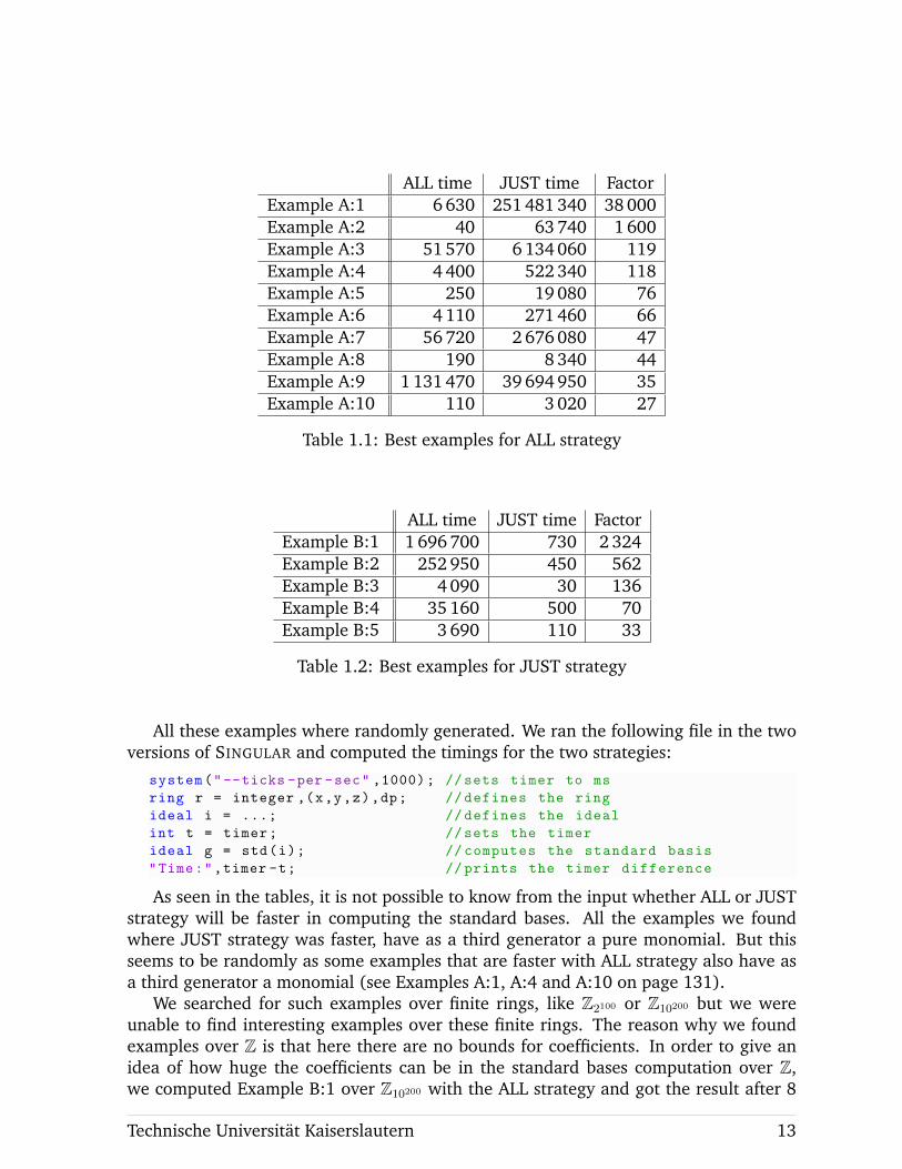
ALL time JUST time FactorExample A:1 6 630 251 481 340 38 000Example A:2 40 63 740 1 600Example A:3 51 570 6 134 060 119Example A:4 4 400 522 340 118Example A:5 250 19 080 76Example A:6 4 110 271 460 66Example A:7 56 720 2 676 080 47Example A:8 190 8 340 44Example A:9 1 131 470 39 694 950 35Example A:10 110 3 020 27
Table 1.1: Best examples for ALL strategy
ALL time JUST time FactorExample B:1 1 696 700 730 2 324Example B:2 252 950 450 562Example B:3 4 090 30 136Example B:4 35 160 500 70Example B:5 3 690 110 33
Table 1.2: Best examples for JUST strategy
All these examples where randomly generated. We ran the following file in the twoversions of SINGULAR and computed the timings for the two strategies:
system("--ticks -per -sec" ,1000); //sets timer to ms
ring r = integer ,(x,y,z),dp; // defines the ring
ideal i = ...; // defines the ideal
int t = timer; //sets the timer
ideal g = std(i); // computes the standard basis
"Time:",timer -t; // prints the timer difference
As seen in the tables, it is not possible to know from the input whether ALL or JUSTstrategy will be faster in computing the standard bases. All the examples we foundwhere JUST strategy was faster, have as a third generator a pure monomial. But thisseems to be randomly as some examples that are faster with ALL strategy also have asa third generator a monomial (see Examples A:1, A:4 and A:10 on page 131).
We searched for such examples over finite rings, like Z2100 or Z10200 but we wereunable to find interesting examples over these finite rings. The reason why we foundexamples over Z is that here there are no bounds for coefficients. In order to give anidea of how huge the coefficients can be in the standard bases computation over Z,we computed Example B:1 over Z10200 with the ALL strategy and got the result after 8
Technische Universitat Kaiserslautern 13
seconds; over Z101000 we obtained the result after 648 seconds (10 minutes) and over Zwe got the result after almost 30 hours. One can imagine how big the coefficients arewhen computing over Z[x]. This is the main reason why in some cases, the computationof a standard basis over Z will be slow.
A:1.4 Huge coefficients over the integers
One of the most common problems when computing over Z[x] is that the coefficientswill rapidly increase. If during the algorithm we have two polynomials with big coeffi-cients, when computing their s−polynomial (or strong polynomials) we multiply themwith the corresponding monomials, and hence the coefficients will become larger. Thiswill slow down the algorithm and increase the memory usage. In order to keep thecoefficients as small as possible we have implemented some easy tricks.
SINGULAR ’s polynomial reduction procedure reduce(f, g) only reduces f by g ifLT(g) divides LT(f). So, if f and g are equal to
f = 78 234 678 956 783 785 656 788 689 · x13y19 + 987 237 527 429 289 · x5y11
g = 1 024 · x2y10,
then the result of reduce(f, g) will be equal to f . But that is a huge waste of memorysince we could simply use f mod g = x13y19 − 423 · x5y11 afterwards. Not only thisaffects the coefficients of f but will also cause smaller coefficients of s-poly(f,−) andgcd-poly(f,−).
We examined several examples for which SINGULAR hanged before, most of the timebecause it ran out of memory, and tested them against the new strategies with positiveresults. Despite that, the most interesting one of them (we will refer to this as Example18 − can be found in the Appendix on page 133), the resulting standard basis wassmall enough (9 polynomials with maximum length 3 and 2 digit coefficients) and evencontained a constant. After checking Example 18 we observed that it took a lot of timeuntil a monomial (or constant) would have entered the partial standard basis (line 6 inAlgorithm A:1.2.10). As before, this gave rise to big coefficients filling the memory up.With the help of G. Pfister and D. Popescu, we implemented a way to access a constant(or a monomial) early in the algorithm. This we explain in the following.
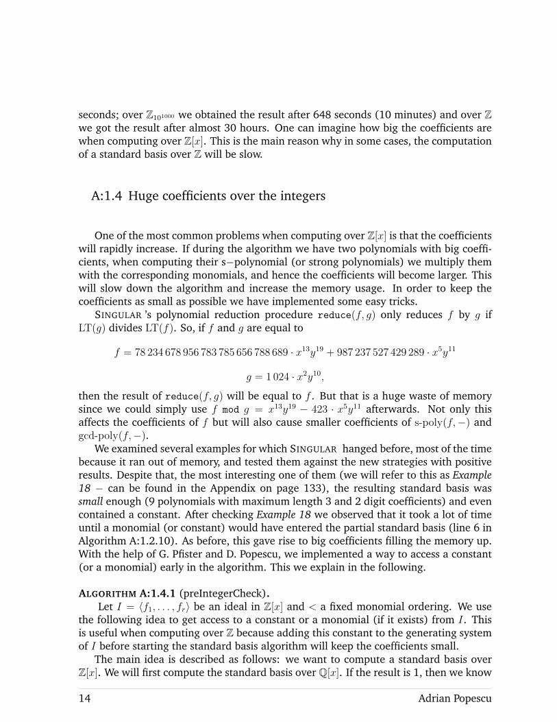
ALGORITHM A:1.4.1 (preIntegerCheck).Let I = 〈f1, . . . , fr〉 be an ideal in Z[x] and < a fixed monomial ordering. We use
the following idea to get access to a constant or a monomial (if it exists) from I. Thisis useful when computing over Z because adding this constant to the generating systemof I before starting the standard basis algorithm will keep the coefficients small.
The main idea is described as follows: we want to compute a standard basis overZ[x]. We will first compute the standard basis over Q[x]. If the result is 1, then we know
14 Adrian Popescu
there is a constant in the ideal and we can get access to it by using some SINGULAR
tricks.
Algorithm preIntegerCheck(ideal I)1: J = {1, f1, . . . , fr}2: compute S, a standard basis of I over Q[x]
3: compute the syzygies Z ⊂r⊕i=0
Q[x] · εi of J
4: if S = 〈1〉 then5: search in Z for a syzygy where the 0 component consists of just a constant c · ε06: return I ∪ {c}7: else8: search in Z for a syzygy where the 0 component consists of just a term c ·m · ε09: if such monomial is found then
10: return I ∪ {c ·m}11: return I
Note that Algorithm A:1.4.1 is very costly and in the case when the algorithm doesn’tfind a constant or monomial, it increases the standard basis run-time without bringingany new information. However in the other cases, the algorithms run-time will improvebecause we have a bound on the coefficients. This is very useful over Z since the biggestproblem proves to be the size of the coefficients that appear during the standard basiscomputation.
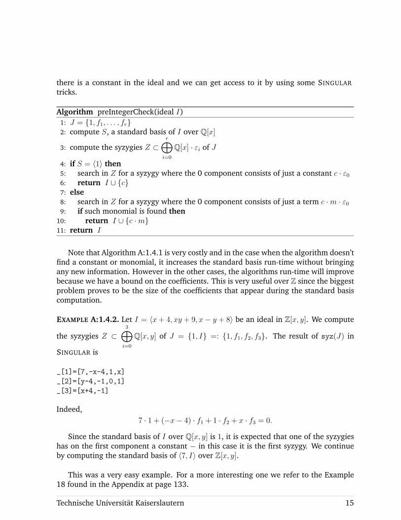
EXAMPLE A:1.4.2. Let I = 〈x+ 4, xy + 9, x− y + 8〉 be an ideal in Z[x, y]. We compute
the syzygies Z ⊂3⊕i=0
Q[x, y] of J = {1, I} =: {1, f1, f2, f3}. The result of syz(J) in
SINGULAR is
_[1]=[7,-x-4,1,x]
_[2]=[y-4,-1,0,1]
_[3]=[x+4,-1]
Indeed,7 · 1 + (−x− 4) · f1 + 1 · f2 + x · f3 = 0.
Since the standard basis of I over Q[x, y] is 1, it is expected that one of the syzygieshas on the first component a constant − in this case it is the first syzygy. We continueby computing the standard basis of 〈7, I〉 over Z[x, y].
This was a very easy example. For a more interesting one we refer to the Example18 found in the Appendix at page 133.
Technische Universitat Kaiserslautern 15
A:1.5 Strong pairs in the reduction procedure
During testing, another interesting example came to our attention. Recall the defi-nition of a normal form A:1.2.7.
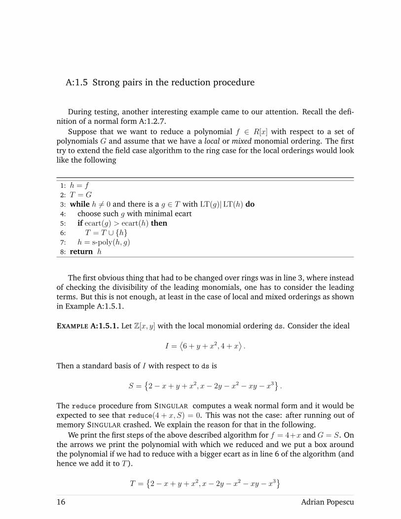
Suppose that we want to reduce a polynomial f ∈ R[x] with respect to a set ofpolynomials G and assume that we have a local or mixed monomial ordering. The firsttry to extend the field case algorithm to the ring case for the local orderings would looklike the following
1: h = f2: T = G3: while h 6= 0 and there is a g ∈ T with LT(g)|LT(h) do4: choose such g with minimal ecart5: if ecart(g) > ecart(h) then6: T = T ∪ {h}7: h = s-poly(h, g)8: return h
The first obvious thing that had to be changed over rings was in line 3, where insteadof checking the divisibility of the leading monomials, one has to consider the leadingterms. But this is not enough, at least in the case of local and mixed orderings as shownin Example A:1.5.1.
EXAMPLE A:1.5.1. Let Z[x, y] with the local monomial ordering ds. Consider the ideal
I =⟨6 + y + x2, 4 + x
⟩.
Then a standard basis of I with respect to ds is
S ={
2− x+ y + x2, x− 2y − x2 − xy − x3}.
The reduce procedure from SINGULAR computes a weak normal form and it would beexpected to see that reduce(4 + x, S) = 0. This was not the case: after running out ofmemory SINGULAR crashed. We explain the reason for that in the following.
We print the first steps of the above described algorithm for f = 4+x and G = S. Onthe arrows we print the polynomial with which we reduced and we put a box aroundthe polynomial if we had to reduce with a bigger ecart as in line 6 of the algorithm (andhence we add it to T ).
T ={
2− x+ y + x2, x− 2y − x2 − xy − x3}
16 Adrian Popescu
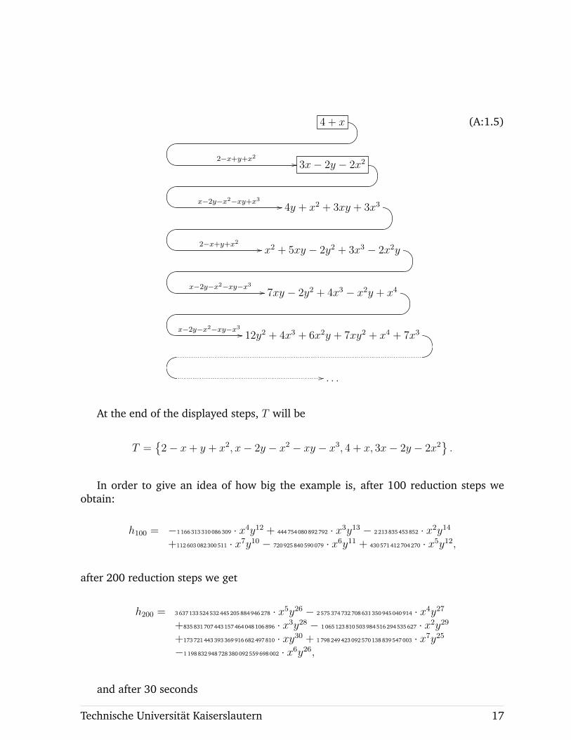
4 + x
2−x+y+x2 // 3x− 2y − 2x2
x−2y−x2−xy+x3 // 4y + x2 + 3xy + 3x3
2−x+y+x2 // x2 + 5xy − 2y2 + 3x3 − 2x2y
x−2y−x2−xy−x3 // 7xy − 2y2 + 4x3 − x2y + x4
x−2y−x2−xy−x3 // 12y2 + 4x3 + 6x2y + 7xy2 + x4 + 7x3
// . . .
(A:1.5)
At the end of the displayed steps, T will be
T ={
2− x+ y + x2, x− 2y − x2 − xy − x3, 4 + x, 3x− 2y − 2x2}.
In order to give an idea of how big the example is, after 100 reduction steps weobtain:
h100 = −1 166 313 310 086 309 · x4y12 + 444 754 080 892 792 · x3y13 − 2 213 835 453 852 · x2y14+112 603 082 300 511 · x7y10 − 720 925 840 590 079 · x6y11 + 430 571 412 704 270 · x5y12,
after 200 reduction steps we get
h200 = 3 637 133 524 532 445 205 884 946 278 · x5y26 − 2 575 374 732 708 631 350 945 040 914 · x4y27+835 831 707 443 157 464 048 106 896 · x3y28 − 1 065 123 810 503 984 516 294 535 627 · x2y29+173 721 443 393 369 916 682 497 810 · xy30 + 1 798 249 423 092 570 138 839 547 003 · x7y25−1 198 832 948 728 380 092 559 698 002 · x6y26,
and after 30 seconds
Technische Universitat Kaiserslautern 17
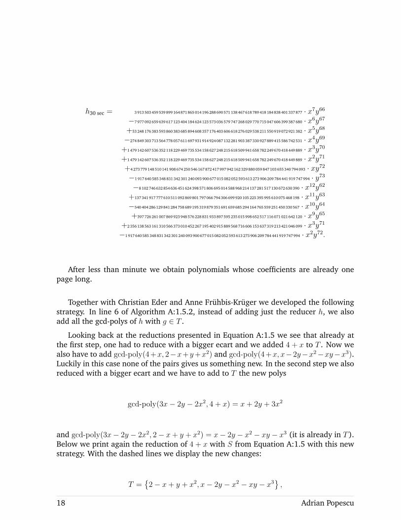
h30 sec = 3 913 503 459 539 899 164 871 865 014 196 288 690 571 138 467 618 789 418 184 838 401 337 877 · x7y66−7 977 092 659 639 617 123 404 184 624 123 573 036 579 747 268 029 770 715 047 606 399 387 680 · x6y67+53 248 176 383 593 860 383 685 894 608 357 176 403 606 618 276 029 538 211 550 919 072 921 382 · x5y68−274 849 303 713 564 778 057 611 697 931 914 924 087 132 281 903 387 330 927 889 415 586 742 531 · x4y69
+1 479 142 607 536 352 118 229 469 735 534 158 627 248 215 618 509 941 658 782 249 670 418 449 889 · x3y70+1 479 142 607 536 352 118 229 469 735 534 158 627 248 215 618 509 941 658 782 249 670 418 449 889 · x2y71+4 273 779 148 510 141 908 674 250 546 167 872 417 997 942 162 329 880 059 847 103 655 340 794 093 · xy72−1 917 640 585 348 831 342 301 240 093 900 677 015 082 052 593 613 273 906 209 784 441 919 747 994 · y73−8 102 746 632 854 636 451 624 398 571 806 695 014 588 968 214 137 281 517 130 672 630 390 · x12y62
+137 341 917 777 610 511 092 869 801 797 066 794 306 699 920 105 225 395 995 610 075 468 198 · x11y63−540 404 286 129 841 284 758 689 195 319 879 351 691 659 685 294 164 765 559 251 450 330 567 · x10y64+397 726 261 007 869 923 948 576 228 831 933 897 595 235 015 998 652 517 116 071 021 642 120 · x9y65
+2 356 138 563 161 310 566 373 010 452 267 195 402 915 889 568 716 606 153 637 319 213 421 046 099 · x3y71−1 917 640 585 348 831 342 301 240 093 900 677 015 082 052 593 613 273 906 209 784 441 919 747 994 · x2y72.
After less than minute we obtain polynomials whose coefficients are already onepage long.
Together with Christian Eder and Anne Fruhbis-Kruger we developed the followingstrategy. In line 6 of Algorithm A:1.5.2, instead of adding just the reducer h, we alsoadd all the gcd-polys of h with g ∈ T .
Looking back at the reductions presented in Equation A:1.5 we see that already atthe first step, one had to reduce with a bigger ecart and we added 4 + x to T . Now wealso have to add gcd-poly(4+x, 2−x+y+x2) and gcd-poly(4+x, x−2y−x2−xy−x3).Luckily in this case none of the pairs gives us something new. In the second step we alsoreduced with a bigger ecart and we have to add to T the new polys
gcd-poly(3x− 2y − 2x2, 4 + x) = x+ 2y + 3x2
and gcd-poly(3x− 2y − 2x2, 2− x+ y + x2) = x− 2y − x2 − xy − x3 (it is already in T ).Below we print again the reduction of 4 + x with S from Equation A:1.5 with this newstrategy. With the dashed lines we display the new changes:
T ={
2− x+ y + x2, x− 2y − x2 − xy − x3},
18 Adrian Popescu
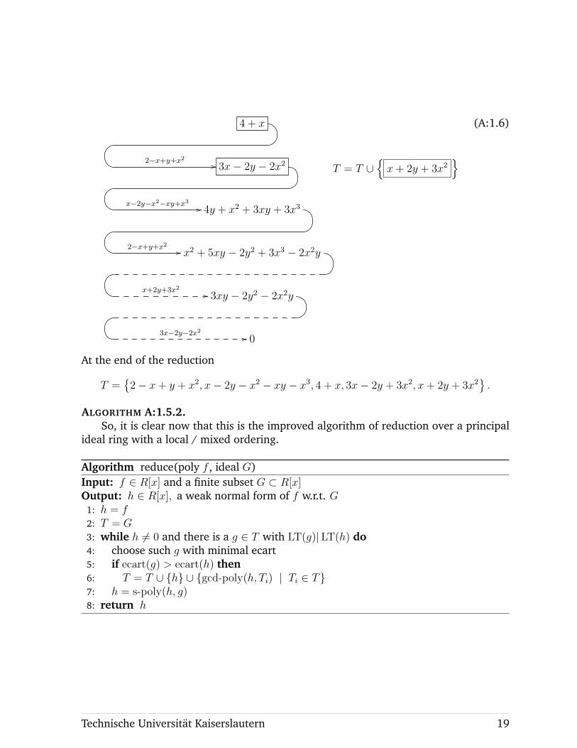
4 + x
2−x+y+x2 // 3x− 2y − 2x2
x−2y−x2−xy+x3 // 4y + x2 + 3xy + 3x3
2−x+y+x2 // x2 + 5xy − 2y2 + 3x3 − 2x2y
x+2y+3x2 // 3xy − 2y2 − 2x2y
3x−2y−2x2 // 0
T = T ∪{x+ 2y + 3x2
}(A:1.6)
At the end of the reduction
T ={
2− x+ y + x2, x− 2y − x2 − xy − x3, 4 + x, 3x− 2y + 3x2, x+ 2y + 3x2}.
ALGORITHM A:1.5.2.So, it is clear now that this is the improved algorithm of reduction over a principal
ideal ring with a local / mixed ordering.
Algorithm reduce(poly f , ideal G)Input: f ∈ R[x] and a finite subset G ⊂ R[x]Output: h ∈ R[x], a weak normal form of f w.r.t. G
1: h = f2: T = G3: while h 6= 0 and there is a g ∈ T with LT(g)|LT(h) do4: choose such g with minimal ecart5: if ecart(g) > ecart(h) then6: T = T ∪ {h} ∪ {gcd-poly(h, Ti) | Ti ∈ T}7: h = s-poly(h, g)8: return h
Technische Universitat Kaiserslautern 19

CHAPTER A:2
SIGNATURE STANDARD BASES OVER THE INTEGERS
This chapter is a joint work with Christian Eder. Here we extend a variant of theF5 Algorithm (see [F]) by first considering the field case as a foundation and thengeneralizing it for rings.
Looking at Buchberger’s Algorithm for computing Grobner bases in Algorithm A:1.2.10,we see that one computes many s-polynomials and not all of these bring new informa-tion to our standard basis. In fact, just a small percentage of these computations willend with a non-zero polynomial. F5 uses several criteria to detect some of these uselesscomputation. To be more specific, this criteria detects if some s−polynomial will reduceto 0 before computing. The idea proves to be very useful because it doesn’t just avoidconstructing new s−polynomials but also prevents the reduction to 0 of these uselesspairs − which is a very time consuming process.
Christian Eder has successfully implemented in SINGULAR a variant of F5 for fieldsby using the Syzygy Criterion, Rewrite Criterion and F5C (see [EP]).
The following sections consist of the problems that arise over principal ideal ringsand their resolution. At the end the resulted algorithm proves to be not as optimal as inthe field case, but we still managed to find some interesting examples.
Throughout this chapter we have to think of the F5 algorithm as being the Grobnerbasis algorithm presented in Algorithm A:1.2.10 to which we add signatures for eachpolynomial in the computation.
A:2.1 Definitions and notations
Faugere had the idea (see [F]) to add to each polynomial a so-called signature − amodule monomial − in order to detect irrelevant s−polynomials before even construct-ing them. This will theoretically increase the memory usage (with the size of a modulemonomial for each polynomial occurring in the computations), but the running timewill decrease in most of the field examples.
As before, let R be a ring, R[x] the polynomial ring in n variables x1, . . . , xn shortlydenoted by x and I = 〈f1, . . . , fm〉 a finitely generated ideal in R[x]. Let R[x]m be thefree module generated by ε1, . . . , εm and π the projection
π : R[x]m // R[x]
εi� // fi
(A:2.1)
Technische Universitat Kaiserslautern 21
REMARK A:2.1.1.
1. For each element f in I, there is a element F ∈ R[x]m such that π(F ) = f . This is
easily proven by taking the linear combination f =m∑i=1
pi · fi and lifting it to get
F =m∑i=1
pi · εi. Note that F is not necessarily unique, since f can be represented
in multiple linear combinations.
2. The elements of ker(π) are syzygies of I.
In this chapter we use as the module ordering ≺:= (C,<) (see Example A:1.1.15)for a global monomial ordering < on R[x]. We extend the module ordering ≺ to modulemonomials with coefficients:
c1 · xα1 ≺ c2 · xα2 ⇐⇒ xα1 ≺ xα2 orxα1 = xα2 and |c1| < |c2|,
where by |c| we denote the absolute value for c ∈ R.Our purpose is to compute a Grobner basis for I.
DEFINITION A:2.1.2 (Signatures).Let f ∈ R[x] be a polynomial that appears in the Grobner basis algorithm (Algorithm
A:1.2.10). We enhance f by giving it a signature, denoted by sig(f). This is a modulemonomial with coefficient defined as follows:
• for an input polynomial fi, we set
sig(fi) = 1 · εi,
• for a s−polynomial of f, g ∈ R[x] denoted by
p := s-poly(f, g) = cfmf · f − cgmg · g,
where cf , cg ∈ R and mf ,mg are monomials in R[x] corresponding to the s-polycomputation, we define the signature as
sig(p) = LT≺(cfmf · sig(f)− cgmg · sig(g)),
• we define it similarly for the gcd−polynomials.
The details concerning the signature of the extended s−polynomials will follow inSection A:2.5. For now, let us consider R = Z.
In the following example we consider Buchberger’s blueprint (Algorithm A:1.2.10)while adding these signature. It is very important for the termination and future criteria
22 Adrian Popescu
to consider each time the polynomial with the smallest signature w.r.t. ≺. In fact, weassume that at each step, the partial standard basis is a standard basis up to the currentsignature. This means that if we added to our partial standard basis S a polynomial fi,all polynomials p with sig(p) ≺ sig(fi) will reduce to 0 with respect to S. In other words,the signature of each newly added polynomial to the standard basis will be greater (orequal) to the previous one. This is crucial for the criteria, without which the algorithmwill significantly slow down. We revisit this subject in Section A:2.3.
When working with signatures, the first problem that arises is in the reduction step.We defined the signature for the initial elements, the s−polynomials and the gcd−polynomials. Because of the need to have increasing signature, the reduce procedurefrom Algorithm A:1.5.2 will have to be updated.
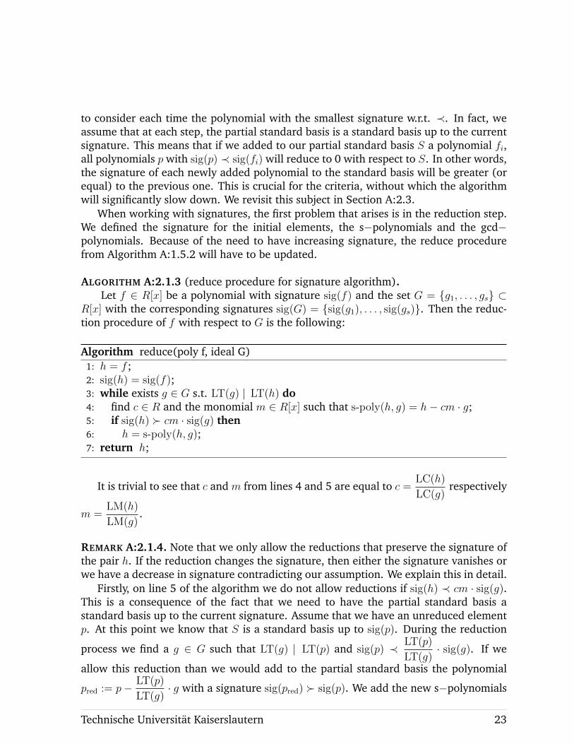
ALGORITHM A:2.1.3 (reduce procedure for signature algorithm).Let f ∈ R[x] be a polynomial with signature sig(f) and the set G = {g1, . . . , gs} ⊂
R[x] with the corresponding signatures sig(G) = {sig(g1), . . . , sig(gs)}. Then the reduc-tion procedure of f with respect to G is the following:
Algorithm reduce(poly f, ideal G)1: h = f ;2: sig(h) = sig(f);3: while exists g ∈ G s.t. LT(g) | LT(h) do4: find c ∈ R and the monomial m ∈ R[x] such that s-poly(h, g) = h− cm · g;5: if sig(h) � cm · sig(g) then6: h = s-poly(h, g);7: return h;
It is trivial to see that c and m from lines 4 and 5 are equal to c =LC(h)
LC(g)respectively
m =LM(h)
LM(g).
REMARK A:2.1.4. Note that we only allow the reductions that preserve the signature ofthe pair h. If the reduction changes the signature, then either the signature vanishes orwe have a decrease in signature contradicting our assumption. We explain this in detail.
Firstly, on line 5 of the algorithm we do not allow reductions if sig(h) ≺ cm · sig(g).This is a consequence of the fact that we need to have the partial standard basis astandard basis up to the current signature. Assume that we have an unreduced elementp. At this point we know that S is a standard basis up to sig(p). During the reduction
process we find a g ∈ G such that LT(g) | LT(p) and sig(p) ≺ LT(p)
LT(g)· sig(g). If we
allow this reduction than we would add to the partial standard basis the polynomial
pred := p− LT(p)
LT(g)· g with a signature sig(pred) � sig(p). We add the new s−polynomials
Technische Universitat Kaiserslautern 23
and gcd−polynomials (with signature greater or equal than sig(p′)). It may happen thatthere is already in the pair list L an earlier element s with sig(p) � sig(s) ≺ sig(p′).If we cannot reduce this element it would be added to the partial standard basis andcontradict the assumption of our algorithm − that the signature of the new element hasto be greater or equal than the signature of the previous element.
Secondly, it may happen that the signatures on line 5 are equal. Then the signatureswill cancel out and our new element will not have a proper signature. We call this asigdrop.
The first idea we had to overcome this second case was instead of considering justthe leading term of the module element (i.e. the signature) we have stored the wholemodule element. We have implemented this strategy in SINGULAR and we noticed thatthis strategy proves to be ineffective. For once, it is used much more memory − insteadof saving just the leading term, we save the whole module element (which can bearbitrary big). Moreover, as in the previous case, the assumption of the partial standardbasis being a standard basis up to the current signature would be violated. Indeed, letthe module element corresponding to h be
H := cm · sig(g) + c1m1 · εi + . . . ∈ R[x]m
and the module element corresponding to g be
G := sig(g) + c2m2 · εj + . . . ∈ R[x]m.
Then the module element corresponding to the reduced h, denoted by h′ = h− c · g, is
H ′ = c2cm2m · εj + c1m1 · εi + . . . .
Assume now that sig(h′) = c2cm2m ·εj ≺ sig(h) and we add h′ to the partial standardbasis and build the s−pairs. The next element that will be added to S (or even this one)may have a smaller signature as the previous one, contradicting our assumption.
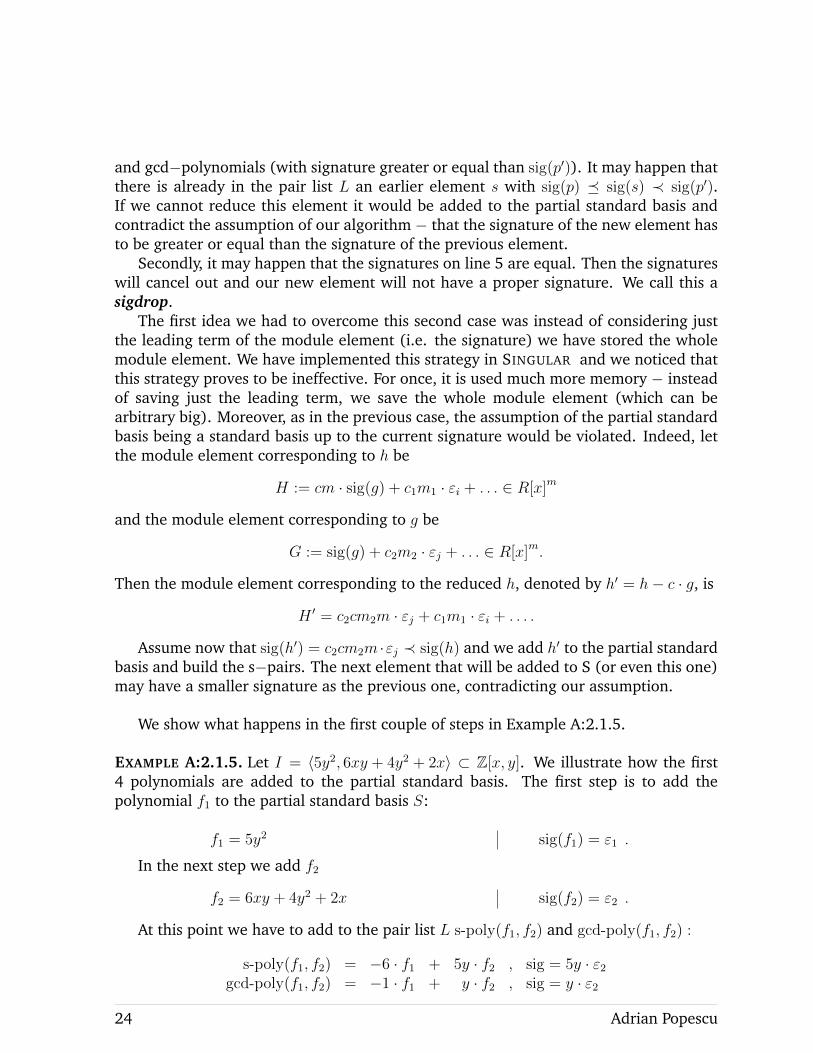
We show what happens in the first couple of steps in Example A:2.1.5.
EXAMPLE A:2.1.5. Let I = 〈5y2, 6xy + 4y2 + 2x〉 ⊂ Z[x, y]. We illustrate how the first4 polynomials are added to the partial standard basis. The first step is to add thepolynomial f1 to the partial standard basis S:
f1 = 5y2 sig(f1) = ε1 .
In the next step we add f2
f2 = 6xy + 4y2 + 2x sig(f2) = ε2 .
At this point we have to add to the pair list L s-poly(f1, f2) and gcd-poly(f1, f2) :
s-poly(f1, f2) = −6 · f1 + 5y · f2 , sig = 5y · ε2gcd-poly(f1, f2) = −1 · f1 + y · f2 , sig = y · ε2
24 Adrian Popescu
Since the signature of the gcd−polynomial is smaller, gcd-poly(f1, f2) will be consid-ered in the next step:
f3 := gcd-poly(f1, f2) = xy2 + 4y3 + 2xy sig(f3) = y · ε2 .
Hence we have to add s-poly(f3, f1), gcd-poly(f3, f1), s-poly(f3, f2) and gcd-poly(f3, f2)to the pair list L. Since both of the gcd−polynomials are redundant we only need toadd the polynomials below to the pair list:
s-poly(f3, f1) = 5 · f3 − x · f1 , sig = 5yε2s-poly(f3, f2) = 6 · f3 − y · f2 , sig = 6y · ε2 − y · ε2 = 5y · ε2
(A:2.2)
At this point the pair list L contains three pairs, all having the same signature 5y · ε2.In fact all three polynomials are equal to 20y3 + 10xy and therefore it doesn’t actuallymatter which we consider first. After we reduce it with f1, we add it to the partialstandard basis:
f4 := s-poly(f2, f3) = 10xy sig(f4) = 5y · ε2 .
REMARK A:2.1.6. When working over a field, the signature of a s−polynomials-poly(f, g) is set to be max {cfmf · sig(f), cgmg · sig(g)}. Unfortunately, this isn’t trueover rings (see Equation A:2.2 from Example A:2.1.5). The reason is that over fields wedo not need coefficients in the signature since we can always set the leading coefficientto be 1 by multiplying with it’s inverse.
A:2.2 Criteria: Syzygy, Rewrite and F5C
This section contains several criteria used over fields in SINGULAR ’s source code andhow we can extend them to rings.
A very useful criteria over fields is the syzygy criterion. This will take advantageof the already zero−reductions and delete further pairs. The proof over fields extendsautomatically over rings. The difficult problem over rings is to assure that the partialstandard basis is a standard basis up to the current signature. We show the difficulty inExample A:2.2.19.
LEMMA A:2.2.1(Syzygy Criterion
).
Assume that in Algorithm A:2.1.3 we have reduced a polynomial s to 0 withsig(s) = cm · εi 6= 0. Let f a polynomial from the pair set L with sig(f) � sig(s). Ifsig(s) | sig(f), then f will reduce to 0.
Technische Universitat Kaiserslautern 25
Proof.Since sig(s) | sig(f) it implies sig(f) = cm · sig(s). Denote the modules elements
corresponding to s and f by S = sig(s) + . . . respectively F = sig(f) + . . . and let themodule element P := F − cm · S with LT(P ) ≺ sig(f). Because the partial standardbasis is a standard basis up to sig(f) and since LT(P ) is strictly smaller than sig(f),we know that π(P ) will reduce to 0 via the partial standard basis. Since S is a syzygy,π(P ) = π(F − cm · S) = π(F ) = f . Therefore we proved that f reduces to 0.
REMARK A:2.2.2. Note that we can use the Syzygy Criterion when building thes−polynomial or the gcd−polynomial. We can first compute it’s signature and if wefind a syzygy that divides this signature, then we can delete the pair.
REMARK A:2.2.3. The Syzygy Criterion proves to be very useful, as we already knowsome initial syzygies. Assume in our partial standard basis we have two elements f1 andf2, with sig(f1) = ε1 and sig(f2) = ε2. In this case a natural syzygy is LT(f1) · ε2. This isbecause π(f1 · ε2 − f2 · ε1) = f1 · f2 − f2 · f1 = 0.
In general, if the polynomials fi have the signatures sig(fi) = εi for 1 ≤ i ≤ n, thenwe can add to the initial syzygies the following set
{LT(fj) · εk | j = 1, . . . , n− 1 and j < k ≤ n} .
We explain this in the following example.
EXAMPLE A:2.2.4. This example represents a continuation of Example A:2.1.5. Denoteby Syz the set consisting in the leading terms of the found syzygies. At this point wehave the initial syzygy (see Remark A:2.2.3):
Syz ={
5y2 · ε2}.
Recall the first steps from Example A:2.1.5:
f1 = 5y2 sig(f1) = ε1f2 = 6xy + 4y2 + 2x sig(f2) = ε2f3 := gcd-poly(f1, f2) = xy2 + 4y3 + 2xy sig(f3) = y · ε2f4 := s-poly(f2, f3) = 10xy sig(f4) = 5y · ε2
We previously added f4 and the pair list L consists in the new s-poly(f4, fi) andgcd-poly(f4, fi) for i = 1, 2, 3:
gcd-poly(f4, f2) = −2 · f2 + f4 , sig = 5y · ε2s-poly(f4, f1) = −10xy · f1 + 5y2 · f4 , sig = 25y3 · ε2s-poly(f4, f2) = −5 · f2 + 3 · f4 , sig = 15y · ε2s-poly(f4, f3) = −10 · f3 + y · f4 , sig = 5y2 · ε2
The first element deleted with the syzygy criterion is s-poly(f4, f1), since it has signa-ture sig = 25y3 ·ε2 and we have one syzygy with the leading term dividing the signature.In this case the s-poly(f4, f1) is trivially already 0.
26 Adrian Popescu
However, we cannot delete s-poly(f4, f3) that has signature sig = 5y2 · ε2 because wein the proof we needed that the syzygy’s signature is strictly smaller than the signatureof the considered pair.
The pair with the smallest signature in the pair list is gcd-poly(f4, f2) and hence weadd it to the partial standard basis:
f5 := gcd-poly(f2, f4) = −2xy − 8y2 − 4x sig(f5) = 5y · ε2 .
With f5 being added to the partial standard basis, we have to add the correspondingnew pairs to the pair list:
gcd-poly(f1, f5) = x · f1 + 2y · f5 , sig = 10y2 · ε2s-poly(f1, f5) = 2x · f1 + 5y · f5 , sig = 25y2 · ε2s-poly(f2, f5) = f2 + 3 · f5 , sig = 15y · ε2s-poly(f3, f5) = 2 · f3 + y · f5 , sig = 5y2 · ε2s-poly(f4, f5) = f4 + 5 · f5 , sig = 30y · ε2
Note that we can already delete gcd-poly(f1, f5) and s-poly(f1, f5) because of thesyzygy criterion.
For the next step, we consider the pair with smallest signature in L. In our case15y · ε2 and after we reduce it with f1, we add it to the partial standard basis.
f6 := s-poly(f2, f5) = −10x sig(f5) = 15y · ε2 .
Note that all the new pairs will be deleted by the syzygy criterion:
gcd-poly(f2, f6) = 2 · f2 + y · f6 , sig = 15y2 · ε2s-poly(f1, f6) = 10x · f1 + 5y2 · f6 , sig = 75y3 · ε2s-poly(f2, f6) = 5 · f2 + 3y · f6 , sig = 45y2 · ε2s-poly(f3, f6) = 10 · f3 + y2 · f6 , sig = 15y3 · ε2s-poly(f4, f6) = f4 + y · f6 , sig = 15y2 · ε2s-poly(f5, f6) = −5 · f5 + y · f6 , sig = 15y2 · ε2
Now the pair list consists of:
L = {s-poly(f3, f5), s-poly(f4, f5), s-poly(f2, f4), s-poly(f3, f4)} .
But all of these will reduce to 0.
REMARK A:2.2.5. Over fields, it can be easily proven that each signature appears onlyonce, i.e. if there are two pairs having the same signature, then we can randomlypick one of them. This is not true over rings, as shown in Example A:2.2.4: f4 andf5 have the same signature. We need f5 in our standard basis. In this case f5 is thegcd−polynomial of f4 and f2. One suspects that this may happen just for the gcd−pairs.The next examples illustrates that this is false. Also completely independent pairs canhave the same signature over integers.
Technische Universitat Kaiserslautern 27
EXAMPLE A:2.2.6. Let I = 〈4x4, 4x3 + 2x2 + 4x〉 ⊂ Z[x] be an ideal. These are all poly-nomials added to S in the signature based algorithm:
f1 = 4x4 sig = ε1f2 = 4x3 + 2x2 + 4x sig = ε2f3 = s-poly(f1, f2) = 2x3 + 4x2 sig = x · ε2f4 = s-poly(f2, f3) = 6x2 − 4x sig = 2x · ε2f5 = s-poly(f1, f3) = −4x2 − 8x sig = 2x2 · ε2f6 = s-poly(f3, f4) = −16x2 sig = 2x2 · ε2f7 = s-poly(f2, f4) = −10x2 − 4x sig = 2x2 · ε2f8 = gcd-poly(f4, f5) = 2x2 − 12x sig = 2x2 · ε2f9 = s-poly(f2, f4) = −14x2 − 12x sig = 4x2 · ε2f10 = gcd-poly(f4, f9) = −2x2 − 20x sig = 4x2 · ε2f11 = s-poly(f4, f5) = −32x sig = 6x2 · ε2
Note that f5, f6, f7 and f8 have the same signature.After we complete reduce the standard basis we obtain G = {2x2 − 12x, 32x} =
{f8,−f11} and see that the standard basis consists just of the s-poly and gcd-poly of thesame two polynomials. This is unusual and shows once again that we need both pairsin the signature based algorithm even if they may have the same signature.
A method for the F5 algorithm that we can extend with ease to the ring case is theF5C strategy developed by Eder and Perry in [EP]. This is a step in the incrementalapproach in computing standard basis when using the position over terms ordering(C,<). We present this in the following algorithm.
ALGORITHM A:2.2.7 (F5C).Let I = 〈f1, . . . , fn〉 ⊂ R[x] be an ideal. We can compute a standard basis S of I
incrementally by using this algorithm.
Algorithm F5C(f1, . . . , fn)1: S = {f1, ext-poly(f1)}; //partial standard basis2: L = ∅; //pair list3: i=2;4: while i < n do5: L = {s-poly(fi, g) | g ∈ S} ∪ {gcd-poly(fi, g) | g ∈ S} ∪ {ext-poly(fi)};6: compute the standard basis of S ∪ {fi} by starting F5 with the pair-set L;7: completely reduce S without considering signatures;8: i = i+ 1;9: return G;
By completely reduce it is understood that we only consider those elements fromthe standard basis whose leading terms are not divisible by other leading terms (i.e.
28 Adrian Popescu
a minimal standard basis is computed). As stated before the signatures block someof the reductions and for instance we may obtain at the end of F5 the following twopolynomials: 10x2y and 2xy with some signatures that will block the zero-reduction. Itis clear that the first one brings no new information for the standard basis.
Because of line 7, many polynomials will be deleted from S and therefore fewerpairs will be considered in the next loop of the algorithm.
We continue by explaining the algorithm in detail. After computing the standardbasis S on line 6 with F5, we reduce it to Sred without considering the signatures. Afterthis step the old signatures become unusable and therefore we need to reset them.
Assume that we are in the i−th loop of the algorithm. Denote the previous S fromline 5 by Si−1 = {g1, . . . , gn}. Then we would add fi to Si−1 and compute a signaturestandard basis of Si−1 ∪ {fi} by adding just the pairs as seen in line 5. At the end of thiscomputation the current partial standard basis will be Si = {g1, . . . , gn, fi, h1, . . . , hs}.After the reduction from line 7, Sred
i = {g′1, . . . , g′t} and we set S = Sredi with the reseted
signatures sig(g′i) = εi.We show how the strategy works in the following example.
EXAMPLE A:2.2.8. We continue with an enhanced version of Example A:2.2.6. We addto the ideal I the polynomial 14x5 + 3x, and we compute the standard basis of
I =⟨4x4, 4x3 + 2x2 + 4x, 14x5 + 3x
⟩= 〈F1, F2, F3〉 .
This new element gets a new signature ε3, and hence the order of the polynomialsfrom Example A:2.2.6 will remain unmodified. Next we show the differences caused byF5C. We print a table with the standard basis S and the pair list L. On the left columnis the next step without F5C and on the right side we can see the benefits of F5C.
without F5C with F5C
S
f1 = F1 = 4x4 sig = ε1f2 = F2 = 4x3 + 2x2 + 4x sig = ε2f3 = 2x3 + 4x2 sig = x · ε2f4 = 6x2 − 4x sig = 2x · ε2f5 = −4x2 − 8x sig = 2x2 · ε2f6 = −16x2 sig = 2x2 · ε2f7 = −10x2 − 4x sig = 2x2 · ε2f8 = 2x2 − 12x sig = 2x2 · ε2f9 = −14x2 − 12x sig = 4x2 · ε2f10 = −2x2 − 20x sig = 4x2 · ε2f11 = −32x sig = 6x2 · ε2f12 = F3 = 14x5 + 3x sig = ε3
f1 = 2x2 − 12x sig = ε1f2 = −32x sig = ε2f3 = F3 = 14x5 + 3x sig = ε3
Technische Universitat Kaiserslautern 29
From this we can immediately see the advantages of F5C even for such a smallexample. Instead of adding 11 s−polynomials and 7 gcd−polynomials to the pair set Lwe only add 2 s-poly and 1 gcd-poly.
REMARK A:2.2.9. Looking back at Example A:2.2.8 we see another advantage of theF5C: better syzygies are added.
In the run without F5C, after adding F3 to our standard basis, we have the initialsyzygies:
Syzno F5C ={
4x4 · ε2, 4x4 · ε3, 4x3 · ε3},
and in the variant with F5C we obtain
Syzwith F5C ={
2x2 · ε2, 2x2 · ε3, 32x · ε3}.
One can immediately see that Syzwith F5C are better since they delete more pairs thanSyzno F5C.
An easy trick in optimizing F5 over rings that we have implemented is the following.
LEMMA A:2.2.10(Gcd Pair Replace
).
Assume that in the F5 algorithm we consider a pair p with signature sig(p). Let S ={f1, . . . , fs} be the partial standard basis up to this step. If there exists a polynomialf ∈ S such that gcd-poly(p, f) has signature equal to sig(p), then we can replace p withgcd-poly(p, f).
Proof.First of all, note that if such an fi exists and we would add p to S, then gcd-poly(p, fi)
would be the pair considered in the next step in the algorithm because it has the samesignature as p. Since gcd-poly(p, f) has the same signature as p, then gcd-poly(p, f) =p− cm · f , for c ∈ R and m a monomial in R[x].
Next we prove that all s−polynomials and gcd−polynomials q between p and an-other element g ∈ S can be reduced using gcd-poly(p, f) to 0. Then q could be writtenas
q := cpmp · p− cgmg · g.
But we can also consider the pair between g and gcd-poly(p, f) of the form
q′ := cpmp · gcd-poly(p, f)− cgmg · g = cpmp · (p− cm · f)− cgmg · g = q − cpcmpm · f.
Note that it is obvious that we can consider only q′.
This idea can be integrated in the reduction procedure for the signature based algo-rithm F5 (Algorithm A:2.1.3).
30 Adrian Popescu
ALGORITHM A:2.2.11.The following procedure will search if for a polynomial p there exists f ∈ S as in
Lemma A:2.2.10.
Algorithm sbaCheckGcdReplace(poly p, ideal S)1: for f ∈ S do2: if sig
(gcd-poly(p, f)
)= sig(p) then
3: return gcd-poly(p, f)4: return p
Now the reduction procedure for the signature algorithm (Algorithm A:2.1.3) canbe updated to the following.
◦ On the first line, we replace f by sbaCheckGcdReplace(f , S)
◦ Before returning h, (i.e. no more reductions found), we replace h bysbaCheckGcdReplace(h,S), and if this is a new polynomial, try again the reductionprocedure.
In fact, we can add to the reduction procedure the strategy presented in SectionA:1.4 where pure monomials were used to shorten the coefficients of polynomials. Be-cause we are working with signatures, we only allow the reductions where the signaturewill not change.
The following example illustrates the benefits of the strategy presented in LemmaA:2.2.10.
EXAMPLE A:2.2.12. Let I = 〈28y2, 16x2 + 7xy〉 =: {F1, F2} ⊂ Z[x, y] be an ideal. Thebox contains the element that vanishes during the run of the algorithm with the strategyfrom Lemma A:2.2.10 enabled.
f1 = F1 = 28y2 sig = ε1f2 = F2 = 16x2 + 7xy sig = ε2f3 = gcd-poly(f1, f2) = 4x2y2 + 14xy3 sig = 2y2 · ε2f4 = s-poly(f1, f2) = 21xy3 sig = 7y2 · ε2f5 = gcd-poly(f4, f1) = −7xy3 sig = 7y2 · ε2f6 = s-poly(f1, f3) = 14xy3 sig = 14y2 · ε2f7 = gcd-poly(f4, f3) = x2y3 sig = 7xy2 · ε2f8 = gcd-poly(f2, f6) = −2x2y3 sig = 14xy2 · ε2f9 = gcd-poly(f4, f2) = −x2y3 sig = 21xy2 · ε2
In this case the only element that can be replaced is f4, and therefore all pairs with f4are irrelevant. This is a small example, in larger examples the benefits of this approachby shortening the pair list L and the partial standard basis S are more obvious. Thisexample also illustrates the main disadvantage in working with signatures: when using
Technische Universitat Kaiserslautern 31
the normal Buchberger Algorithm, instead of f7, f8, f9 we would simply have f7, butwith the F5 Algorithm, we cannot reduce f8 with f7. If we allow this reduction theresult would look like
f8 + 2 · f7
with signature 28xy2 · ε2, and hence the signature would increase, contradicting ourassumption. For the same reason we cannot reduce f9 with f7.
REMARK A:2.2.13. An idea that comes in mind to avoid adding irrelevant elements tothe partial standard bases such as f8, f9 in the previous example would be to reducealways reduce them without considering the signature.
Another important criteria that deletes useless pairs in the field case is the RewriteCriterion. In this we use the signature of the polynomial that have been already addedto the partial standard basis. The proof in the field case can be found in [EP].
LEMMA A:2.2.14(Rewrite Criterion
).
Let S = {f1, . . . , fs} be a partial signature standard basis and p := s-poly(fi, fj).Assume that there exists a fk ∈ S such that sig(fk) | sig(p) and i, j ≤ k. Then p containsno new information since we can rewrite it using the actual standard basis. In other words,we can delete this pair from L.
The proof uses the fact that the signature of a s−polynomial s-poly(f, g) is either amultiple of sig(f) or a multiple of sig(g). But over rings, as seen in Remark A:2.1.6, thisdoes not hold, and will cause the deletion of critical pairs needed by the algorithm asshown in the following example.
EXAMPLE A:2.2.15. Let I = 〈8y2, 4x2y + 5y3 + 7y2 + 9x〉 be an ideal in Z[x, y] with thedp ordering. Assume that we use the Rewrite Criterion also over rings. In the followingwe show each polynomial that is added to the standard basis.
f1 = 8y2 sig = ε1f2 = 4x2y + 5y3 + 7y2 + 9x sig = ε2f3 = gcd-poly
(s-poly(f1, f2), f1
)= 2y4 + 14y3 + 18xy sig = 2y · ε2
f4 = s-poly(f3, f1) = 72xy sig = 8y · ε2f5 = gcd-poly
(s-poly(f2, f4), f1
)= −2y3 − 126y2 − 162x sig = 8xy · ε2
f6 = s-poly(f1, f5) = −648x sig = 32xy · ε2f7 = gcd-poly
(s-poly(f2, f3), f3
)= −y6 + 28x2y3 + 5y5 + 36x3y + 27xy3 sig = 4x2y · ε2
The next critical pair that should go in the standard basis would be
f8 = s-poly(f2, f5) = 5y5 − 252x2y2 + 7y4 − 324x3 + 9xy2 sig = 16x3y · ε2,
32 Adrian Popescu
but this is deleted by the Rewrite Criterion: sig(f7) | sig(f8), 2 < 7 and 5 < 7; andtherefore leads to an incorrect standard basis, instead of the correct one:
648 · x,8 · y2,72 · xy,2 · y3 + 126 · y2 + 162 · x,4 · x2y + 5 · y3 + 7 · y2 + 9 · x,y5 − 324 · x3 − 315 · xy2 − 3 969 · y3 − 5 103 · xy.
Because of the deleted polynomial, we cannot reconstruct the last polynomial, whichwould be gcd-poly(f8, f3) with sig = 16x3y · ε2.
Unfortunately we were unable to develop a version of Rewrite Criterion that wouldcorrectly function over rings.
We are now ready to continue the idea from Remark A:2.1.4 concerning the sigdrop.When working over a field, Rewrite Criterion deletes the pairs before they would comeinto a situation where the signature would vanish. Therefore in the case of fields, thereare no signature drops.
REMARK A:2.2.16. Recall that in the field case, all the polynomials and signature havethe leading coefficient 1.
In fact, the field version of the Rewrite Criterion is the following:Let fi, fj ∈ S be two polynomials in the partial standard basis, mi = LM(fi), mj =
LM(fj), L = lcm(mi,mj) such that
s-poly(fi, fj) =L
mi
· fi −L
mj
· fj =: λi · fi − λj · fj.
If there is an fk with k ≥ i, j such that sig(fk) | λi · sig(fi) or sig(fk) | λj · sig(fj), thenwe can delete s-poly(fi, fj).
LEMMA A:2.2.17.Over fields, the signature of a s−polynomial will never vanish.
Proof.Assume we have a s−polynomial for which the signature vanishes. Using the nota-
tion from the previous remark,
s-poly(fi, fj) = λi · fi − λj · fj,
andλi · sig(fi) = λj · fj.
Assume that sig(fi) ≺ sig(fj) (i.e. i < j). Then we can apply the Rewrite Criterion forfi and delete the pair.
Technische Universitat Kaiserslautern 33
In the ring case this does not hold, as the following easy example reveals.
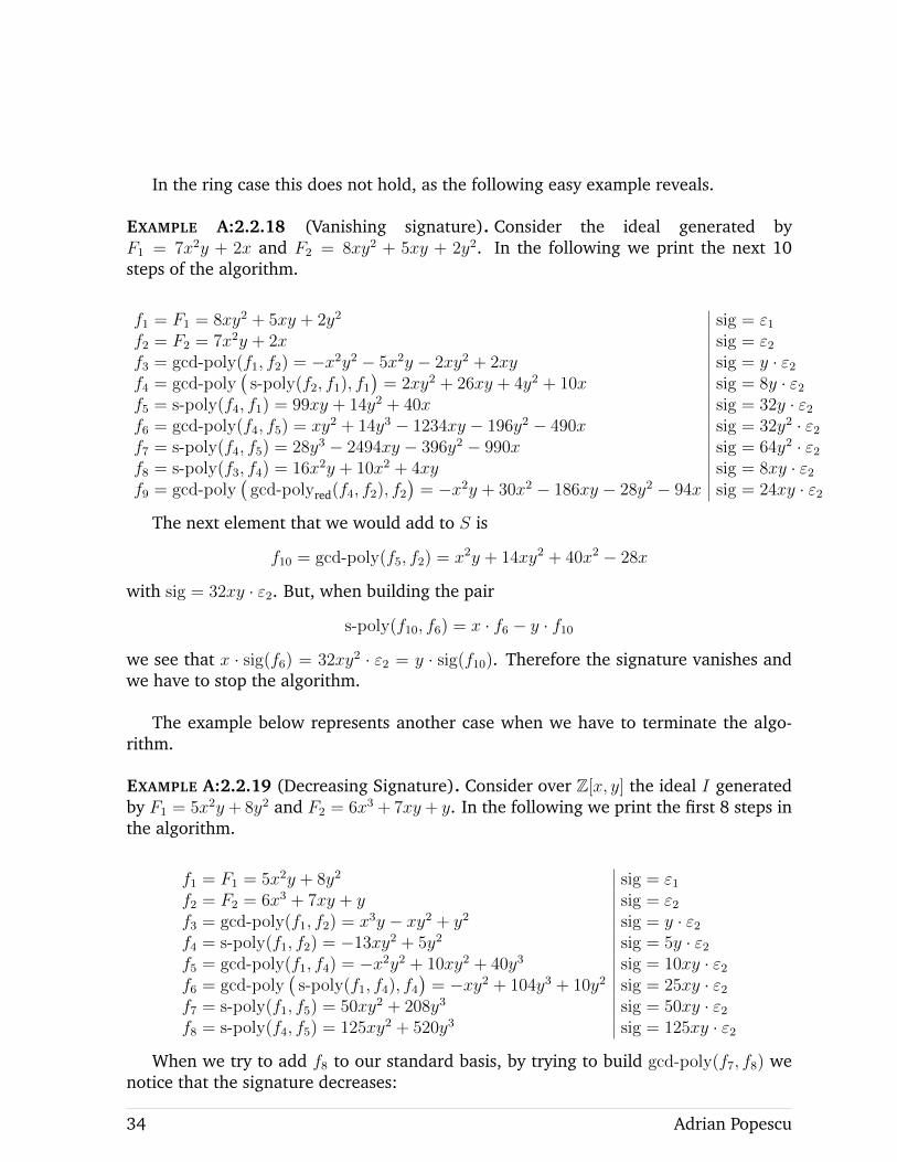
EXAMPLE A:2.2.18 (Vanishing signature). Consider the ideal generated byF1 = 7x2y + 2x and F2 = 8xy2 + 5xy + 2y2. In the following we print the next 10steps of the algorithm.
f1 = F1 = 8xy2 + 5xy + 2y2 sig = ε1f2 = F2 = 7x2y + 2x sig = ε2f3 = gcd-poly(f1, f2) = −x2y2 − 5x2y − 2xy2 + 2xy sig = y · ε2f4 = gcd-poly
(s-poly(f2, f1), f1
)= 2xy2 + 26xy + 4y2 + 10x sig = 8y · ε2
f5 = s-poly(f4, f1) = 99xy + 14y2 + 40x sig = 32y · ε2f6 = gcd-poly(f4, f5) = xy2 + 14y3 − 1234xy − 196y2 − 490x sig = 32y2 · ε2f7 = s-poly(f4, f5) = 28y3 − 2494xy − 396y2 − 990x sig = 64y2 · ε2f8 = s-poly(f3, f4) = 16x2y + 10x2 + 4xy sig = 8xy · ε2f9 = gcd-poly
(gcd-polyred(f4, f2), f2
)= −x2y + 30x2 − 186xy − 28y2 − 94x sig = 24xy · ε2
The next element that we would add to S is
f10 = gcd-poly(f5, f2) = x2y + 14xy2 + 40x2 − 28x
with sig = 32xy · ε2. But, when building the pair
s-poly(f10, f6) = x · f6 − y · f10
we see that x · sig(f6) = 32xy2 · ε2 = y · sig(f10). Therefore the signature vanishes andwe have to stop the algorithm.
The example below represents another case when we have to terminate the algo-rithm.
EXAMPLE A:2.2.19 (Decreasing Signature). Consider over Z[x, y] the ideal I generatedby F1 = 5x2y + 8y2 and F2 = 6x3 + 7xy + y. In the following we print the first 8 steps inthe algorithm.
f1 = F1 = 5x2y + 8y2 sig = ε1f2 = F2 = 6x3 + 7xy + y sig = ε2f3 = gcd-poly(f1, f2) = x3y − xy2 + y2 sig = y · ε2f4 = s-poly(f1, f2) = −13xy2 + 5y2 sig = 5y · ε2f5 = gcd-poly(f1, f4) = −x2y2 + 10xy2 + 40y3 sig = 10xy · ε2f6 = gcd-poly
(s-poly(f1, f4), f4
)= −xy2 + 104y3 + 10y2 sig = 25xy · ε2
f7 = s-poly(f1, f5) = 50xy2 + 208y3 sig = 50xy · ε2f8 = s-poly(f4, f5) = 125xy2 + 520y3 sig = 125xy · ε2
When we try to add f8 to our standard basis, by trying to build gcd-poly(f7, f8) wenotice that the signature decreases:
34 Adrian Popescu
gcd-poly(f7, f8) = −2 · f7 + f8 = 25xy2 + 104y3,
sig(
gcd-poly(f7, f8))
= 25xy · ε2 ≺ 125xy · ε2 = sig(f8).
This decreasing signature, from now on referred to as a sigdrop, will cause us to endthe algorithm, because we would contradict the assumption that the partial standardbasis is a standard basis up to the current signature.
A:2.3 SigDrops
In the previous section we have seen that over rings, sigdrops occur and that theylead to the termination of the algorithm since otherwise it could return an incorrectresult. This section describes what can be done after a sigdrop occurs.
We give a trivial example that happens often in a signature standard basis compu-tation over rings. Assume that we added to S a polynomial fp := s-poly(fi, fj) withsignature sig(fp) and that in the next step we consider the same polynomial with thesame signature but from a different pair s-poly(fk, fl) = fp. We do not want to addthe same polynomial with the same signature in the partial standard basis, but usingthe reduction procedure shown in Algorithm A:2.1.3, we see that we cannot reduces-poly(fk, fl) by fp since they have the same signature and it would vanish causing asigdrop. A solution to this would be to also let reduction when the signatures are equaland whenever we have sigdrops (caused by vanishing signature as in Example A:2.2.18or a decreased signature as in Example A:2.2.19), we reduce the polynomial with thereduction procedure from the normal Buchberger Algorithm without considering thesignatures. If after this reduction the polynomial is 0, we can continue with the algo-rithm − since it was an irrelevant element. However, if after the reduction the elementis still non zero, then we have to terminate the algorithm.
After these sigdrops, we have to restart the algorithm with the partial standard basisbut with reinitialized new signatures. As we saw sigdrops can happen either in thereduction step or when building the s−polynomials and gcd−polynomials.
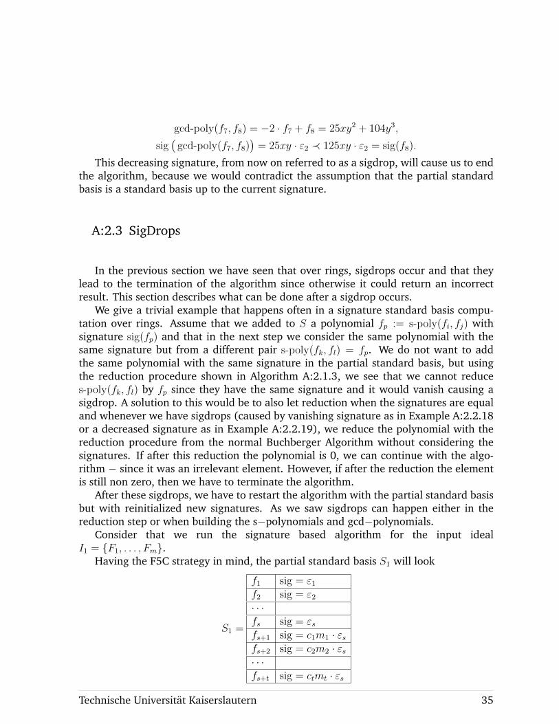
Consider that we run the signature based algorithm for the input idealI1 = {F1, . . . , Fm}.
Having the F5C strategy in mind, the partial standard basis S1 will look
S1 =
f1 sig = ε1f2 sig = ε2· · ·fs sig = εsfs+1 sig = c1m1 · εsfs+2 sig = c2m2 · εs· · ·fs+t sig = ctmt · εs
Technische Universitat Kaiserslautern 35
Assume for the moment that the sigdrop was caused in the easier case − in the re-duction step− and that after trying to reduce the polynomial fs+t+1 without consideringsignatures, it still remains nonzero.
Looking at F5C (or using the idea behind the incremental computation) it is clearthat fs = Fu ∈ I1.
A natural way to continue after this sigdrop is to start again the algorithm with thenew input I2 = {f1, . . . , fs+t+1, Fu+1, . . . , Fm} with new signatures as in F5C and deletemost of the elements in the pair list L1 − since the signatures will change and we willhave to also recompute the signatures of the pairs. The only pairs from L1 that we donot delete are the unused initial polynomials Fu+1, . . . , Fm. These elements have to goagain as initial elements.
REMARK A:2.3.1. Note that we can already add f1, . . . , fs−1 to the partial standard basisS2 since in the previous run all of the pairs between them were either added to S1 orreduced to 0. This holds due to our module ordering (C,<) − all the remaining pairsin L1 have the signature non zero on the s component, and hence it originally had tocome from a pair with fs.
Now we assume that the sigdrop was caused in a pair computation p (s-poly orgcd-poly) between the newly added polynomial fs+t and an fi from the partial standardbasis. In this case, we have to add to I2 also p.
The hard step is to choose an ordering for the elements of I2. This ordering affectsthe new signatures of the polynomials. If we sort them simply by increasing ring mono-mial ordering, as one normally does at a beginning of the signature algorithm, then itmay be possible that we would get to the same sigdrop, and hence the algorithm willbe stuck in an infinite loop. We show in detail such an example.
EXAMPLE A:2.3.2. Consider the ideal I generated by F1 = 5y3 + 8y2 + 6y andF2 = 8x2y+ 9x2 in Z[x, y] with the dp ordering. We print the first steps in the following.
f1 = F1 = 5y3 + 8y2 + 6y sig = ε1f2 = F2 = 8x2y + 9x2 sig = ε2f3 = gcd-poly(f1, f2) = x2y3 − 6x2y2 − 18x2y sig = 2y2 · ε2f4 = s-poly(f1, f2) = −19x2y2 + 54x2 sig = 5y2 · ε2f5 = gcd-poly
(s-poly(f1, f3), f2
)= 2x2y2 − 51x2y sig = 10y2 · ε2
f6 = gcd-poly(
s-poly(f2, f3), f2)
= −x2y2 − 81x2y sig = 15y2 · ε2f7 = s-poly(f2, f4) = 171x2y + 432x2 sig = 40y2 · ε2f8 = s-poly(f2, f5) = −213x2y sig = 40y2 · ε2
The next element considered is
gcd-poly(f4, f5) = −x2y2 − 459x2y + 54x2∣∣ sig = 95y2 · ε2.
We would like to reduce this by f6 to −378x2y + 54x2 which has signature 80y2 · ε2.This would cause a sigdrop since the signature decreased. After reducing as much as we
36 Adrian Popescu
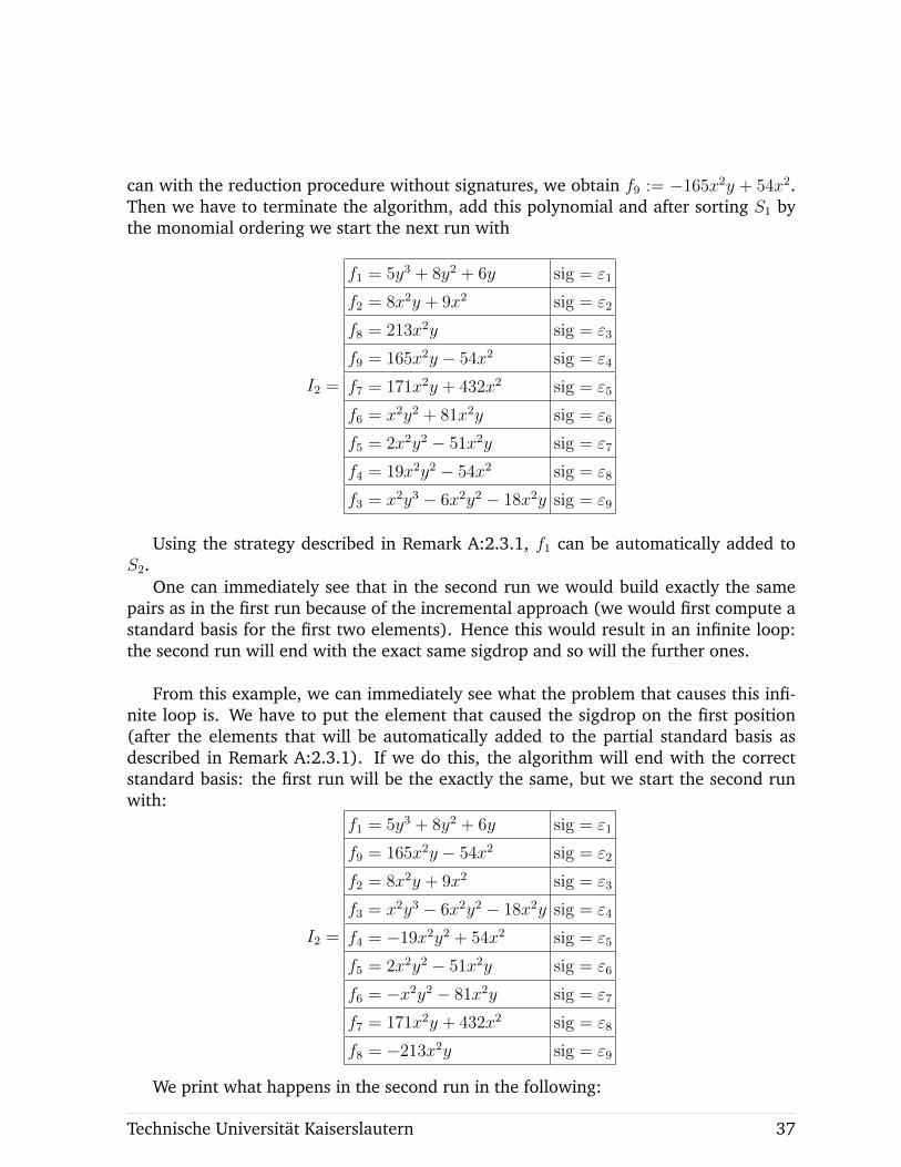
can with the reduction procedure without signatures, we obtain f9 := −165x2y + 54x2.Then we have to terminate the algorithm, add this polynomial and after sorting S1 bythe monomial ordering we start the next run with
I2 =
f1 = 5y3 + 8y2 + 6y sig = ε1
f2 = 8x2y + 9x2 sig = ε2
f8 = 213x2y sig = ε3
f9 = 165x2y − 54x2 sig = ε4
f7 = 171x2y + 432x2 sig = ε5
f6 = x2y2 + 81x2y sig = ε6
f5 = 2x2y2 − 51x2y sig = ε7
f4 = 19x2y2 − 54x2 sig = ε8
f3 = x2y3 − 6x2y2 − 18x2y sig = ε9
Using the strategy described in Remark A:2.3.1, f1 can be automatically added toS2.
One can immediately see that in the second run we would build exactly the samepairs as in the first run because of the incremental approach (we would first compute astandard basis for the first two elements). Hence this would result in an infinite loop:the second run will end with the exact same sigdrop and so will the further ones.
From this example, we can immediately see what the problem that causes this infi-nite loop is. We have to put the element that caused the sigdrop on the first position(after the elements that will be automatically added to the partial standard basis asdescribed in Remark A:2.3.1). If we do this, the algorithm will end with the correctstandard basis: the first run will be the exactly the same, but we start the second runwith:
I2 =
f1 = 5y3 + 8y2 + 6y sig = ε1
f9 = 165x2y − 54x2 sig = ε2
f2 = 8x2y + 9x2 sig = ε3
f3 = x2y3 − 6x2y2 − 18x2y sig = ε4
f4 = −19x2y2 + 54x2 sig = ε5
f5 = 2x2y2 − 51x2y sig = ε6
f6 = −x2y2 − 81x2y sig = ε7
f7 = 171x2y + 432x2 sig = ε8
f8 = −213x2y sig = ε9
We print what happens in the second run in the following:
Technische Universitat Kaiserslautern 37
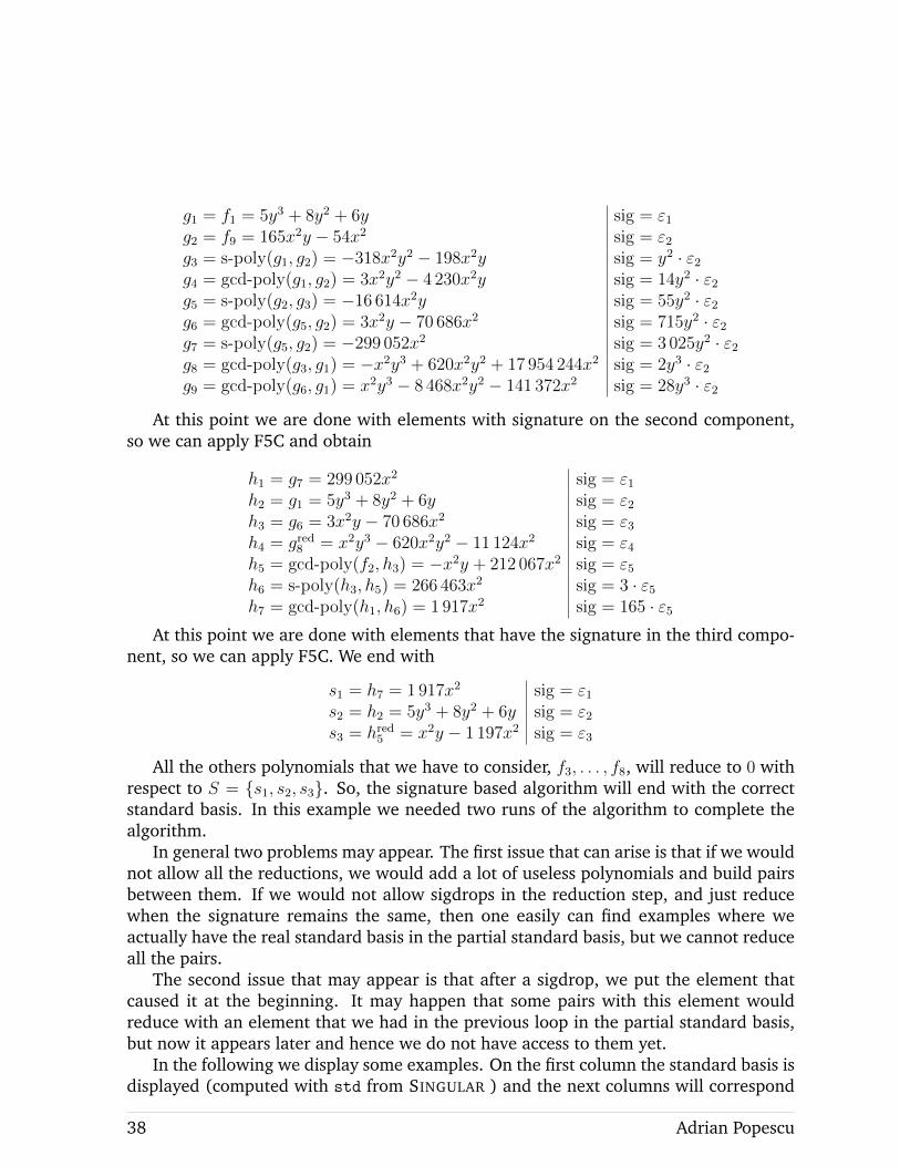
g1 = f1 = 5y3 + 8y2 + 6y sig = ε1g2 = f9 = 165x2y − 54x2 sig = ε2g3 = s-poly(g1, g2) = −318x2y2 − 198x2y sig = y2 · ε2g4 = gcd-poly(g1, g2) = 3x2y2 − 4 230x2y sig = 14y2 · ε2g5 = s-poly(g2, g3) = −16 614x2y sig = 55y2 · ε2g6 = gcd-poly(g5, g2) = 3x2y − 70 686x2 sig = 715y2 · ε2g7 = s-poly(g5, g2) = −299 052x2 sig = 3 025y2 · ε2g8 = gcd-poly(g3, g1) = −x2y3 + 620x2y2 + 17 954 244x2 sig = 2y3 · ε2g9 = gcd-poly(g6, g1) = x2y3 − 8 468x2y2 − 141 372x2 sig = 28y3 · ε2
At this point we are done with elements with signature on the second component,so we can apply F5C and obtain
h1 = g7 = 299 052x2 sig = ε1h2 = g1 = 5y3 + 8y2 + 6y sig = ε2h3 = g6 = 3x2y − 70 686x2 sig = ε3h4 = gred8 = x2y3 − 620x2y2 − 11 124x2 sig = ε4h5 = gcd-poly(f2, h3) = −x2y + 212 067x2 sig = ε5h6 = s-poly(h3, h5) = 266 463x2 sig = 3 · ε5h7 = gcd-poly(h1, h6) = 1 917x2 sig = 165 · ε5
At this point we are done with elements that have the signature in the third compo-nent, so we can apply F5C. We end with
s1 = h7 = 1 917x2 sig = ε1s2 = h2 = 5y3 + 8y2 + 6y sig = ε2s3 = hred5 = x2y − 1 197x2 sig = ε3
All the others polynomials that we have to consider, f3, . . . , f8, will reduce to 0 withrespect to S = {s1, s2, s3}. So, the signature based algorithm will end with the correctstandard basis. In this example we needed two runs of the algorithm to complete thealgorithm.
In general two problems may appear. The first issue that can arise is that if we wouldnot allow all the reductions, we would add a lot of useless polynomials and build pairsbetween them. If we would not allow sigdrops in the reduction step, and just reducewhen the signature remains the same, then one easily can find examples where weactually have the real standard basis in the partial standard basis, but we cannot reduceall the pairs.
The second issue that may appear is that after a sigdrop, we put the element thatcaused it at the beginning. It may happen that some pairs with this element wouldreduce with an element that we had in the previous loop in the partial standard basis,but now it appears later and hence we do not have access to them yet.
In the following we display some examples. On the first column the standard basis isdisplayed (computed with std from SINGULAR ) and the next columns will correspond
38 Adrian Popescu
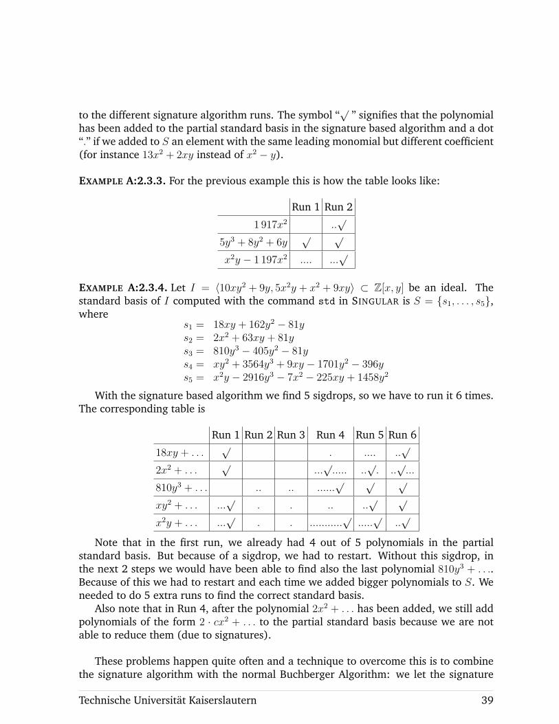
to the different signature algorithm runs. The symbol “√
” signifies that the polynomialhas been added to the partial standard basis in the signature based algorithm and a dot“.” if we added to S an element with the same leading monomial but different coefficient(for instance 13x2 + 2xy instead of x2 − y).
EXAMPLE A:2.3.3. For the previous example this is how the table looks like:
Run 1 Run 2
1 917x2 ..√
5y3 + 8y2 + 6y√ √
x2y − 1 197x2 .... ...√
EXAMPLE A:2.3.4. Let I = 〈10xy2 + 9y, 5x2y + x2 + 9xy〉 ⊂ Z[x, y] be an ideal. Thestandard basis of I computed with the command std in SINGULAR is S = {s1, . . . , s5},where
s1 = 18xy + 162y2 − 81ys2 = 2x2 + 63xy + 81ys3 = 810y3 − 405y2 − 81ys4 = xy2 + 3564y3 + 9xy − 1701y2 − 396ys5 = x2y − 2916y3 − 7x2 − 225xy + 1458y2
With the signature based algorithm we find 5 sigdrops, so we have to run it 6 times.The corresponding table is
Run 1 Run 2 Run 3 Run 4 Run 5 Run 6
18xy + . . .√
. .... ..√
2x2 + . . .√
...√..... ..
√. ..√...
810y3 + . . . .. .. ......√ √ √
xy2 + . . . ...√
. . .. ..√ √
x2y + . . . ...√
. . ...........√
.....√
..√
Note that in the first run, we already had 4 out of 5 polynomials in the partialstandard basis. But because of a sigdrop, we had to restart. Without this sigdrop, inthe next 2 steps we would have been able to find also the last polynomial 810y3 + . . ..Because of this we had to restart and each time we added bigger polynomials to S. Weneeded to do 5 extra runs to find the correct standard basis.
Also note that in Run 4, after the polynomial 2x2 + . . . has been added, we still addpolynomials of the form 2 · cx2 + . . . to the partial standard basis because we are notable to reduce them (due to signatures).
These problems happen quite often and a technique to overcome this is to combinethe signature algorithm with the normal Buchberger Algorithm: we let the signature
Technische Universitat Kaiserslautern 39
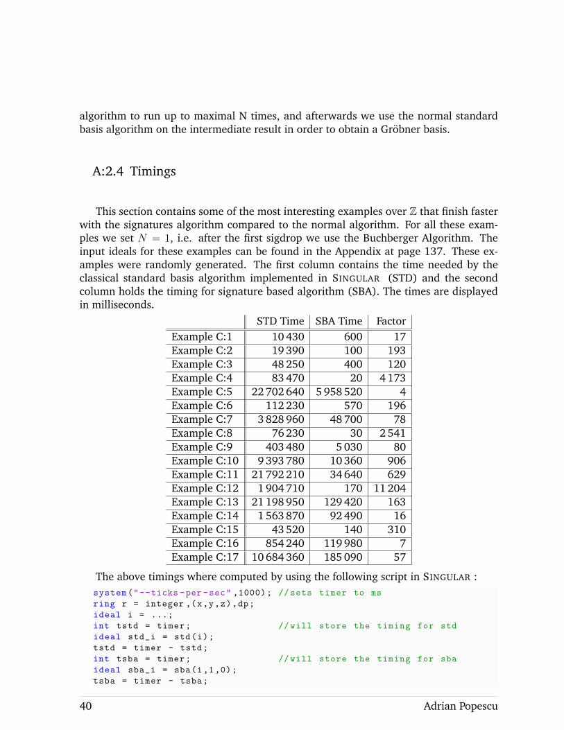
algorithm to run up to maximal N times, and afterwards we use the normal standardbasis algorithm on the intermediate result in order to obtain a Grobner basis.
A:2.4 Timings
This section contains some of the most interesting examples over Z that finish fasterwith the signatures algorithm compared to the normal algorithm. For all these exam-ples we set N = 1, i.e. after the first sigdrop we use the Buchberger Algorithm. Theinput ideals for these examples can be found in the Appendix at page 137. These ex-amples were randomly generated. The first column contains the time needed by theclassical standard basis algorithm implemented in SINGULAR (STD) and the secondcolumn holds the timing for signature based algorithm (SBA). The times are displayedin milliseconds.
STD Time SBA Time FactorExample C:1 10 430 600 17Example C:2 19 390 100 193Example C:3 48 250 400 120Example C:4 83 470 20 4 173Example C:5 22 702 640 5 958 520 4Example C:6 112 230 570 196Example C:7 3 828 960 48 700 78Example C:8 76 230 30 2 541Example C:9 403 480 5 030 80Example C:10 9 393 780 10 360 906Example C:11 21 792 210 34 640 629Example C:12 1 904 710 170 11 204Example C:13 21 198 950 129 420 163Example C:14 1 563 870 92 490 16Example C:15 43 520 140 310Example C:16 854 240 119 980 7Example C:17 10 684 360 185 090 57
The above timings where computed by using the following script in SINGULAR :system("--ticks -per -sec" ,1000); //sets timer to ms
ring r = integer ,(x,y,z),dp;
ideal i = ...;
int tstd = timer; //will store the timing for std
ideal std_i = std(i);
tstd = timer - tstd;
int tsba = timer; //will store the timing for sba
ideal sba_i = sba(i,1,0);
tsba = timer - tsba;
40 Adrian Popescu
In these examples SBA proves to perform much better. The reason for this is thatuntil the sigdrop, we get access to a polynomial that without signatures will take muchmore pairs to obtain. After the sigdrop we continue with STD.
However, in the case when we set N = 1 (just one SBA run is allowed), most exam-ples will finish almost equally fast for the two algorithms. If we set N > 1, then SBAwill become much slower than the STD algorithm for reasons illustrated in ExampleA:2.3.4.
A:2.5 Finite rings − Zm
In the previous sections we have considered R = Z. The strategies, however, holdfor Zm, for a m ∈ N, as well, provided we set also the signature for an extendeds−polynomial. There are two different natural ways to define them.
The first one would be to consider them as completely new elements and assignthem a new signature.
DEFINITION A:2.5.1.For each extended s−polynomial of a polynomial f we enlarge our module with one
more component εm+1 and we set
sig(
ext-poly(f))
= 1 · εm+1.
The second one, takes into consideration the definition of a extended s−polynomial.
DEFINITION A:2.5.2.We set the signature of an extended s−polynomial of a polynomial f = cf ·mf + . . .
bysig(
ext-poly(f))
= Ann(cf ) · sig(f).
Over Zm[x] we will often have sigdrops since we take also coefficients in signaturesin consideration, this signature may become 0 as the next example shows. Because ofthis, the algorithm does not perform well for ideals in Zm[x].
EXAMPLE A:2.5.3. Let R = Z6[x], f = 3x with sig(f) = 3x · ε2 and g = 4x3 + 3x withsig(g) = x · ε2. We want to compute sig
(s-poly(f, g)
). Then
s-poly(f, g) = 4x2 · f − 3 · g = 3x,
and therefore
sig(
s-poly(f, g))
= LT(4x2 · 3x · ε2 + 3 · x · ε2) = LT(3x · ε2) = 3x · ε2.
Technische Universitat Kaiserslautern 41
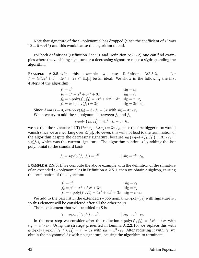
Note that signature of the s−polynomial has dropped (since the coefficient of x3 was12 ≡ 0 mod 6) and this would cause the algorithm to end.
For both definitions (Definition A:2.5.1 and Definition A:2.5.2) one can find exam-ples where the vanishing signature or a decreasing signature cause a sigdrop ending thealgorithm.
EXAMPLE A:2.5.4. In this example we use Definition A:2.5.2. LetI = 〈x5, x4 + x3 + 5x2 + 3x〉 ⊂ Z6[x] be an ideal. We show in the following the first4 steps of the algorithm.
f1 = x5 sig = ε1f2 = x4 + x3 + 5x2 + 3x sig = ε2f3 = s-poly(f1, f2) = 4x3 + 4x2 + 3x sig = x · ε2f4 = ext-poly(f3) = 3x sig = 3x · ε2
Since Ann(4) = 3, ext-poly(f3) = 3 · f3 = 3x with sig = 3x · ε2.When we try to add the s−polynomial between f4 and f3,
s-poly(f4, f3
)= 4x2 · f4 − 3 · f3,
we see that the signature is LT(12x3·ε2−3x·ε2) = 3x·ε2, since the first bigger term wouldvanish since we are working over Z6[x]. However, this will not lead to the termination ofthe algorithm despite the decreasing signature, because sig
(s-poly(f3, f4)
)= 3x · ε2 =
sig(f4), which was the current signature. The algorithm continues by adding the lastpolynomial to the standard basis:
f5 = s-poly(f2, f3) = x2 sig = x2 · ε2,
EXAMPLE A:2.5.5. If we compute the above example with the definition of the signatureof an extended s−polynomial as in Definition A:2.5.1, then we obtain a sigdrop, causingthe termination of the algorithm:
f1 = x5 sig = ε1f2 = x4 + x3 + 5x2 + 3x sig = ε2f3 = s-poly(f1, f2) = 4x3 + 4x2 + 3x sig = x · ε2
We add to the pair list L, the extended s−polynomial ext-poly(f3) with signature ε3,so this element will be considered after all the other pairs.
The next element that will be added to S is
f4 = s-poly(f2, f3) = x2 sig = x2 · ε2,In the next step we consider after the reduction s-poly(f1, f3) = 5x3 + 4x2 with
sig = x3 · ε2. Using the strategy presented in Lemma A:2.2.10, we replace this withgcd-poly
(s-poly(f1, f3), f3
)= x3 + 3x with sig = x3 · ε2. After reducing it with f4, we
obtain the polynomial 3x with no signature, causing the algorithm to terminate.
42 Adrian Popescu

Technische Universitat Kaiserslautern 43


PART B
DEPTH, STANLEY DEPTH AND HILBERT
DEPTH
Technische Universitat Kaiserslautern 45

INTRODUCTION
PART B starts recalling some preliminaries on Cohen−Macaulay Modules, HilbertFunctions and Hilbert Polynomials. Chapter 2 introduces the multigraded Stanley depthand the graded Hilbert depth (shortly sdepthn and hdepth1) presenting also the Stan-ley Conjecture. Afterwards we present an implemented algorithm in SINGULAR thatcomputes the Hilbert Depth published in Journal Symbolic Computation ([AP2]). Sev-eral computational experiments are included. In particular, these show that if R =K[x1, . . . , x6], for a field K, and m = 〈x1, . . . , x6〉, then hdepth1(R ⊕ m) = 4 > 3 =hdepth1(m) (see Remark B:2.2.4). This hints that it might holds also sdepthn(R⊕m) >sdepthn(m), which is a negative solution for a question of J. Herzog. This is indeed thecase as it was stated by B. Ichim and A. Zarojanu in [IZ].
Chapter 3 starts recalling some cases when the multigraded Stanley Conjecture holdsobtained by D. Popescu, A. Zarojanu and Y.H. Shen ([DP5], [PZ],[DP6], [Sh]) in theframe of monomial squarefree ideals. Unfortunately, the multigraded Stanley Conjec-ture does not hold in general as [DuGo] shows (see here Example B:3.1.8). The com-puter algebra system NORMALIZ ([BIS]) uses the multigraded Stanley decomposition tocompute the Hilbert Series. The case when the multigraded Stanley Conjecture failsmakes difficult to find the best multigraded Stanley decomposition and so the compu-tation by NORMALIZ is harder.
Theorem B:3.2.13 (see [AP1]) shows that the Stanley Conjecture holds for intersec-tions of three monomial prime ideals. The proof uses a special decomposition extendedlater by others (see [DP7], [HPV]) under the name of splitting of variables and used forexample in [RTU] and [Ta].
Let J ( I ⊂ R = K[x1, . . . , xn] be monomial square free ideals generated by mono-
mials of degree ≥ d. Then depthI
J≥ d. If among the minimal set of monomial genera-
tors of I there exist at most 3 squarefree monomials of degree d and sdepthnI
J= d+ 1
we show that depthI
J≤ d+ 1 (see Theorem B:3.1.7).
Let G(I), G(J) be the sets of minimal monomial generators of I, respectively J ,where J ( I ⊂ R and di, i ∈ {1, . . . , n} the maximum degree of xi which appearsin a monomial from G(I) ∪ G(J). We say that I/J is in the canonical form if for anyi ∈ {1, . . . , n} and t < di, there exist a monomial from G(I) ∪ G(J) of degree t inxi. In Chapter 4 we introduced a factor of monomial ideals I/J associated to I/J −the canonical form. We have sdepthn I/J = sdepthn I/J by [IKM, Proposition 5.1] (seehere Proposition B:4.0.1) and depthn I/J = depthn I/J by Theorem B:4.1.11. Using thecanonical form, we were able to extend Rinaldo’s Stanley depth algorithm to optimize
Technische Universitat Kaiserslautern 47

the computation of depth and sdepth of I/J using its canonical form. Example B:4.1.13shows that the algorithm is much quicker than the other known ones.
48 Adrian Popescu
CHAPTER B:1
DEFINITIONS AND NOTATIONS
In this chapter we give the definitions and notations that we use throughout thispart. We also try to present examples to better understand notions like Stanley andHilbert depth.
B:1.1 Cohen−Macaulay Modules
In this section we present some connections between the Hilbert functions andCohen−Macaulay rings.
DEFINITION B:1.1.1.We say that an ideal Q ⊂ R is primary if x · y ∈ Q, then x ∈ Q or yn ∈ Q for a
certain n ∈ N. If Q is a primary ideal, then the radical of Q is necessarily a prime idealP , and this ideal is called the associated prime ideal of Q. In this situation, Q is said tobe P−primary.
DEFINITION B:1.1.2.An R−module M is flat if the tensor product functor M ⊗R − is exact. For example
the projective modules, in particular the free ones, are flat modules.
DEFINITION B:1.1.3.Let R be a ring and M a R−module. A sequence x := x1, . . . , xn, xi ∈ R ∀i is called
a M−regular sequence if
◦ xi is not a zero divisor inM
(x1, . . . , xi−1)for i = 1, . . . , n
◦ M
xM6= 0.
In this case n is called the length of x.
REMARK B:1.1.4. If R is a polynomial ring over a field then a regular sequence x of Ris the algebraic analogue of the geometric notion of the complete intersection. Moreprecisely, R/(x) defines a complete intersection if and only if x is regular.
Technische Universitat Kaiserslautern 49
DEFINITION B:1.1.5.Let (R,m) be a Noetherian local ring with m the maximal ideal. The length of a
maximal M−regular sequence x := x1, . . . , xn, for xi ∈ m ∀i is called the depth of M .
REMARK B:1.1.6. If M is a finite R−module then one can define depth by using somenotions from Homological Algebra [BH, Theorem 1.2.5]:
depthM = inf
{n
∣∣∣∣ Extn(R
m,M
)6= 0
}PROPOSITION B:1.1.7
([BH, Propositions 1.2.12, 1.2.13]
).
Let (R,m) be a local Noetherian ring and M a finite generated R−module. ThendepthM ≤ dimM . Moreover, depthM ≤ dim R/P for all P ∈ AssM .
DEFINITION B:1.1.8.Let (R,m) be a local Noetherian ring, and M a R−module. M is called Cohen −
Macaulay module if dimM = depthM or if M = 0.A Noetherian ringR is called a Cohen−Macaulay ring if (R,m) is Cohen−Macaulay
for any maximal ideal m ∈ Max(R).
B:1.2 Hilbert Function and Hilbert Polynomial
The Hilbert function of a graded module associates to an integer n the dimensionof the n−th graded part of a given module. For sufficiently large n, the values of thisfunction can be given by a polynomial, the Hilbert polynomial. To show this, we use theHilbert−Poincare series, a formal power series in t with coefficients being values of theHilbert function.
Throughout this chapter let K be a field.
DEFINITION B:1.2.1.A graded ring R is a ring together with a direct sum decomposition
R =⊕i≥0
Ri,
where the Ri are abelian groups satisfying RiRj ⊂ Ri+j for any i, j ≥ 0.A graded K−algebra is a K−algebra which is a graded ring such that Ri is a
K−vector space for all i ≥ 0 and R0 = K.The Ri are called the homogeneous components and the elements of Ri are called
homogeneous element of degree i.A R−module M , together with a direct sum decomposition
M =⊕i≥0
Mi
50 Adrian Popescu
into abelian groups is called a graded R−module if RiMj ⊂ Mi+j for all i ≥ 0 andj ∈ Z.
LetM =⊕i≥0
Mi be a gradedR−module and defineM(d) :=⊕i∈Z
M(d)i withM(d)i :=
Md+i. Then M(d) is a graded R−module and it is called the d−th shift of M .A submodule N ⊂ M is called a graded submodule if it is generated by ho-
mogeneous elements, or equivalently, if N is graded with the induced grading, i.e.
N =⊕i∈Z
(Mi ∩N).
Let R =⊕i≥0
Ri be a graded ring, M =⊕i∈Z
Mi and N =⊕i∈Z
Ni be two graded
R−modules. A homomorphism ϕ : M → N is called graded of degree d if ϕ(Mi) ⊂ Ni+d
for all i. If ϕ is graded of degree zero, we call ϕ just graded.
DEFINITION B:1.2.2.Let R =
⊕i≥0
Ri be a Noetherian graded K−algebra and let M =⊕i∈Z
Mi be a finitely
generated graded R−module.The Hilbert function HM : Z −→ Z of M is defined by
HM(n) := dimK(Mn).
The Hilbert-Poincare series HPM of M is defined by
HPM(t) :=∑i∈Z
HM(i) · ti ∈ Z JtK[t−1].
Note that the definition of HM and HPM depend only on the graded structure of M .Hence if ϕ : R′ −→ R is a graded K−algebra map, then it does not matter whether weconsider M as a R−module or as a R′−module.
The next results are proven in [BH, Chapter 4].
LEMMA B:1.2.3.Let R =
⊕i≥0
Ri be a Noetherian graded K−algebra and let M be a finitely generated
graded R−module.
1. Let N ⊂M be a graded submodule. Then
HM(n) = HN(n) + HM/N(n)
for all n. In particular HPM(t) = HPN(t) + HPM/N(t).
2. Let d be an integer. ThenHM(d)(n) = HM(n+ d)
for all n. In particular HPM(d)(t) = t−d · HPM(t).
Technische Universitat Kaiserslautern 51
3. Let d be a non-negative integer, let f ∈ Rd and let ϕ : M(−d) −→ M be defined byϕ(m) := f ·m. Then Ker(ϕ) and Coker(ϕ) are graded R/〈f〉−module with the inducedgradings and
HM(n)− HM(n− d) = HCoker(ϕ)(n)− HKer(ϕ)(n− d)
for all n. In particular HPM(t)− td · HPM(t) = HPCoker(ϕ)(t)− td · HPKer(ϕ)(t).
THEOREM B:1.2.4.Let R =
⊕i≥0
Ri be a graded K−algebra and assume that R is generated, as K−algebra,
by x1, . . . , xr ∈ R1. Then for any finitely generated graded R−module M =⊕i≥0
Mi,
HPM(t) =Q(t)
(1− t)r, for some Q(t) ∈ Z[t]. (B:1.1)
With the notations of Theorem B:1.2.4, canceling all common factors from the equa-tion (B:1.1) we obtain
HPM(t) =G(t)
(1− t)s, 0 ≤ s ≤ r, G(t) =
d∑i=0
giti ∈ Z[t], (B:1.2)
such that gd 6= 0 and G(1) 6= 0, that is s is the pole order of HPM(t).
THEOREM B:1.2.5.Let R be a polynomial ring over a field and M 6= 0 be a finite graded R−module of
dimension d. Assume that M is Cohen−Macaulay. Let GM(t) be as in Equation (B:1.2),
GM(t) =∑i
giti. Then gi ≥ 0 for all i.
DEFINITION B:1.2.6.Let R =
⊕i≥0
Ri be a Noetherian graded K−algebra, and let M =⊕i≥0
Mi be a finitely
generated graded R−module.
◦ The polynomials Q(t) and G(t) defined in (B:1.1) and (B:1.2) are called the firstand the second Hilbert series of M .
◦ Let d be the degree of the second Hilbert series G(t) and let s be the pole order ofthe Hilbert-Poincare series HPM(t) at t = 1. Then
PM(n) :=d∑i=0
gi ·(s− 1 + n− i
s− 1
)∈ Q[n], (B:1.3)
where(nk
)= 0 for k < 0, is called the Hilbert polynomial of M .
52 Adrian Popescu
DEFINITION B:1.2.7.Recall Equation (B:1.2). We define the multiplicity of the module M as
e(M) = G(1).
One can prove that e(M) > 0(
see [BH]).
DEFINITION B:1.2.8.Let R be a ring and M be a R−module. The dimension of M is defined by dimM =
dimR
Ann(M).
The length of M , denoted by `(M), is defined to be the largest number n suchthat there exists a chain of submodules of length n, i.e. N0 ( N1 ( . . . ( Nn, for Ni
submodules of M .
REMARK B:1.2.9. Note that in the case of the Hilbert function definition (DefinitionB:1.2.2), Mn were seen as K−vector spaces and then `(Mn) is the dimension of thevectorial space Mn over K.
DEFINITION B:1.2.10.An associated prime of a module M over a ring R is a prime ideal of R of the form
AnnR z for some nonzero z ∈ M . The set of all associated prime ideals is denoted byAssM .
THEOREM B:1.2.11(Hilbert’s Theorem
).
Let M be a finite graded R−module of dimension d. Then HPM(n) is of polynomialtype of degree d− 1.
REMARK B:1.2.12. Theorem B:1.2.11 tells us that the s from (B:1.2) is in fact dimM :
HPM(t) =G(t)
(1− t)dimM.
Recall that e(M) = G(1) > 0.
PROPOSITION B:1.2.13.With the above assumptions, PM is a polynomial in n with rational coefficients, of
degree s − 1, and satisfies PM(n) = HM(n) for n ≥ d. Moreover, there exists ai ∈ Z suchthat
PM(n) =s−1∑i=0
ai ·(n
i
)=
as−1(s− 1)!
· ns−1 + lower terms in n,
where as−1 = G(1) > 0.
Technische Universitat Kaiserslautern 53

CHAPTER B:2
HILBERT DEPTH
B:2.1 Hilbert Series and Hilbert Depth
The results of this chapter are published in [AP2].Let K be a field and R = K[x1 . . . , xn] be the polynomial algebra over K in n vari-
ables. On R consider the following two grading structures:
• the Z−grading in which each xi has degree 1 and
• the multigraded structure, i.e. the Zn−grading, in which each xi has degree thei−th vector ei of the canonical basis.
DEFINITION B:2.1.1.After Bruns-Krattenthaler-Uliczka [BKU] (see also [Sh]), a Hilbert decomposition
of a Z−graded R−module M is a finite family
H = (Ri, si)i∈I
in which si ∈ Z and Ri is a Z−graded K−algebra retract of R for each i ∈ I such that
M ∼=⊕i∈I
Ri(−si)
as a graded K−vector space.
The Hilbert depth ofH denoted by hdepth1H is the depth of theR−module⊕i∈I
Ri(−si).
The Hilbert depth of M is defined as
hdepth1(M) = max{hdepth1H | H is a Hilbert decomposition of M}.
We set hdepth1(0) =∞.It is known that hdepth1(M) ≥ depth(M) (see [BKU]).
DEFINITION B:2.1.2.A Laurent series in Z Jt, t−1K is called positive if it has only non-negative coefficients.
Technische Universitat Kaiserslautern 55
THEOREM B:2.1.3(Uliczka [Uli]
).
hdepth1(M) = max{e | (1− t)e HPM(t) is positive}, where HPM(t) is the Hilbert −Poincare series of M .
If M is a multigraded Zn−module, then one can define hdepthn(M) as above byconsidering the Zn−grading instead of the standard one. There exists an algorithm forcomputing the hdepthn of a finitely generated multigraded module M over the standardmultigraded polynomial ringK[x1, . . . , xn] in Ichim and Moyano-Fernandez’s paper [IM](see also [IZ]).
The main purpose of this chapter is to provide an algorithm to computehdepth1(M), where M is a graded R−module (see Algorithm B:2.1.7). We mentionthat later another such algorithm appeared in [BMU] and containing ours at the refer-ences.
DEFINITION B:2.1.4.A Stanley decomposition (see [St]) of a Z−graded (resp. Zn−graded) R−module
M is a finite familyD = (Ri, ui)i∈I
in which ui are homogeneous elements of M and Ri is a graded (resp. Zn−graded)K−algebra retract of R for each i ∈ I such that Ri ∩ Ann(ui) = 0 and
M =⊕i∈I
Riui
as a graded K−vector space.
The Stanley depth of D denoted by sdepthD is the depth of the R−module⊕i∈I
Riui.
The Stanley depth of M is defined as
sdepth(M) = max{sdepthD | D is a Stanley decomposition of M}.
We set sdepth(0) =∞.The Stanley Conjecture claims that sdepth(M) ≥ depth(M).
We talk about sdepth1(M) and sdepthn(M) if we consider the Z−grading respec-tively the Zn−grading of M . The Hilbert depth of M is greater than the Stanley depthof M and can be strictly greater (an example can be found in [BKU]).
Herzog posed the following question (see also [BGS, Problem 1.67]):
Is sdepthn(R⊕m) = sdepthn(m), where m is the maximal ideal in R?
Since we implemented an algorithm to compute hdepth1, we have tested whetherhdepth1(R⊕m) = hdepth1(m) and as a consequence when sdepthn(R⊕m) = sdepthn(m).
Proposition B:2.2.6 says that Herzog’s question holds for n ∈ {1, . . . , 5, 7, 9, 11}, butRemark B:2.2.4 says that for n = 6 it holds hdepth1(R ⊕ m) > hdepth1m, which is a
56 Adrian Popescu
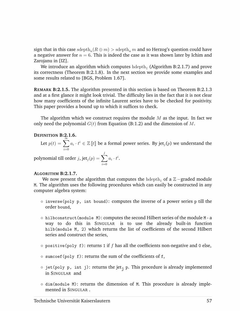
sign that in this case sdepthn(R⊕m) > sdepthnm and so Herzog’s question could havea negative answer for n = 6. This is indeed the case as it was shown later by Ichim andZarojanu in [IZ].
We introduce an algorithm which computes hdepth1 (Algorithm B:2.1.7) and proveits correctness (Theorem B:2.1.8). In the next section we provide some examples andsome results related to [BGS, Problem 1.67].
REMARK B:2.1.5. The algorithm presented in this section is based on Theorem B:2.1.3and at a first glance it might look trivial. The difficulty lies in the fact that it is not clearhow many coefficients of the infinite Laurent series have to be checked for positivity.This paper provides a bound up to which it suffices to check.
The algorithm which we construct requires the module M as the input. In fact weonly need the polynomial G(t) from Equation (B:1.2) and the dimension of M .
DEFINITION B:2.1.6.
Let p(t) =∞∑i=0
ai · ti ∈ Z JtK be a formal power series. By jetj(p) we understand the
polynomial till order j, jetj(p) =
j∑i=0
ai · ti.
ALGORITHM B:2.1.7.We now present the algorithm that computes the hdepth1 of a Z−graded module
M. The algorithm uses the following procedures which can easily be constructed in anycomputer algebra system:
◦ inverse(poly p, int bound): computes the inverse of a power series p till theorder bound,
◦ hilbconstruct(module M): computes the second Hilbert series of the module M - away to do this in SINGULAR is to use the already built-in functionhilb(module M, 2) which returns the list of coefficients of the second Hilbertseries and construct the series,
◦ positive(poly f): returns 1 if f has all the coefficients non-negative and 0 else,
◦ sumcoef(poly f): returns the sum of the coefficients of f,
◦ jet(poly p, int j): returns the jetj p. This procedure is already implementedin SINGULAR and
◦ dim(module M): returns the dimension of M. This procedure is already imple-mented in SINGULAR .
Technische Universitat Kaiserslautern 57
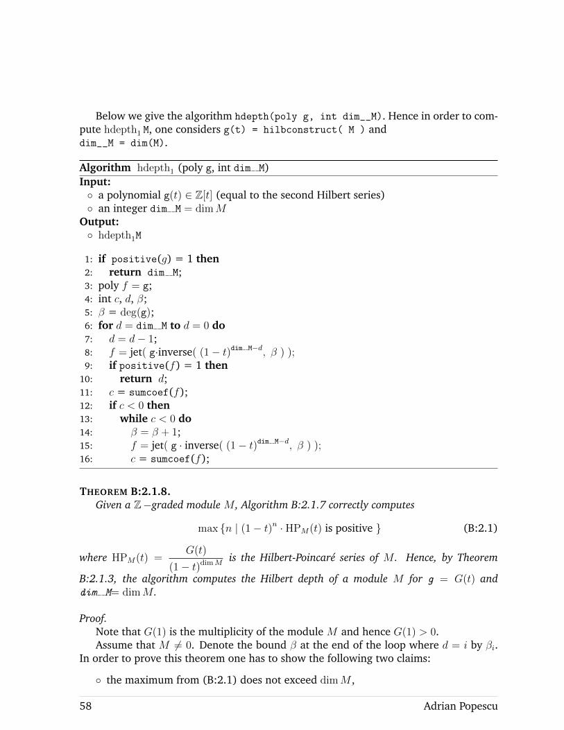
Below we give the algorithm hdepth(poly g, int dim__M). Hence in order to com-pute hdepth1 M, one considers g(t) = hilbconstruct( M ) anddim__M = dim(M).
Algorithm hdepth1 (poly g, int dim M)Input:◦ a polynomial g(t) ∈ Z[t] (equal to the second Hilbert series)◦ an integer dim M = dimM
Output:◦ hdepth1M
1: if positive(g) = 1 then2: return dim M;3: poly f = g;4: int c, d, β;5: β = deg(g);6: for d = dim M to d = 0 do7: d = d− 1;8: f = jet( g·inverse( (1− t)dim M−d, β ) );9: if positive(f) = 1 then
10: return d;11: c = sumcoef(f);12: if c < 0 then13: while c < 0 do14: β = β + 1;15: f = jet( g · inverse( (1− t)dim M−d, β ) );16: c = sumcoef(f);
THEOREM B:2.1.8.Given a Z−graded module M , Algorithm B:2.1.7 correctly computes
max {n | (1− t)n · HPM(t) is positive } (B:2.1)
where HPM(t) =G(t)
(1− t)dimMis the Hilbert-Poincare series of M . Hence, by Theorem
B:2.1.3, the algorithm computes the Hilbert depth of a module M for g = G(t) anddim M= dimM .
Proof.Note that G(1) is the multiplicity of the module M and hence G(1) > 0.Assume that M 6= 0. Denote the bound β at the end of the loop where d = i by βi.
In order to prove this theorem one has to show the following two claims:
◦ the maximum from (B:2.1) does not exceed dimM ,
58 Adrian Popescu
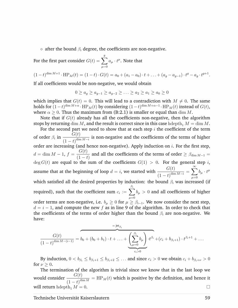
◦ after the bound βi degree, the coefficients are non-negative.
For the first part consider G(t) =
g∑µ=0
aµ · tµ. Note that
(1− t)dimM+1 ·HPM(t) = (1− t) ·G(t) = a0 + (a1− a0) · t+ . . .+ (ag− ag−1) · tg− ag · tg+1.
If all coefficients would be non-negative, we would obtain
0 ≥ ag ≥ ag−1 ≥ ag−2 ≥ . . . ≥ a2 ≥ a1 ≥ a0 ≥ 0
which implies that G(t) = 0. This will lead to a contradiction with M 6= 0. The sameholds for (1− t)dimM+α ·HPM(t) by considering (1− t)dimM+α−1 ·HPM(t) instead of G(t),where α ≥ 0. Thus the maximum from (B:2.1) is smaller or equal than dimM .
Note that if G(t) already has all the coefficients non-negative, then the algorithmstops by returning dimM , and the result is correct since in this case hdepth1M = dimM .
For the second part we need to show that at each step i the coefficient of the term
of order βi inG(t)
(1− t)dimM−i is non-negative and the coefficients of the terms of higher
order are increasing (and hence non-negative). Apply induction on i. For the first step,
d = dimM − 1, f =G(t)
(1− t)and all the coefficients of the terms of order ≥ βdimM−1 =
degG(t) are equal to the sum of the coefficients G(1) > 0. For the general step i,
assume that at the beginning of loop d = i, we started withG(t)
(1− t)dimM−i =∞∑µ=0
bµ · tµ
which satisfied all the desired properties by induction: the bound βi was increased (if
required), such that the coefficient sum ci :=
βi∑µ=0
bµ > 0 and all coefficients of higher
order terms are non-negative, i.e. bµ ≥ 0 for µ ≥ βi−1. We now consider the next step,d = i − 1, and compute the new f as in line 9 of the algorithm. In order to check thatthe coefficients of the terms of order higher than the bound βi are non-negative. Wehave:
G(t)
(1− t)dimM−(i−1) =
= jetβi︷ ︸︸ ︷b0 + (b0 + b1) · t+ . . .+
(βi∑µ=0
bµ
)︸ ︷︷ ︸
ci>0
·tβi +(ci + bβi+1) · tβi+1 + . . .
By induction, 0 < bβi ≤ bβi+1 ≤ bβi+2 ≤ . . . and since ci > 0 we obtain ci + bβi+ν > 0for ν ≥ 0.
The termination of the algorithm is trivial since we know that in the last loop we
would considerG(t)
(1− t)dimM= HPM(t) which is positive by the definition, and hence it
will return hdepth1M = 0.
Technische Universitat Kaiserslautern 59
REMARK B:2.1.9. The maximum from the statement of [Uli, Theorem 3.2] (see hereTheorem B:2.1.3) is always smaller than dimM . This was not shown in Uliczka’s proofand it has to be proved in Theorem B:2.1.8.
B:2.2 Computational Experiments
The following examples illustrate the usage of the implementation of the algorithmin SINGULAR , which can be found in the Section B:2.3. Note that in the outputs weprint exactly the jet we considered in our computations followed by “+...”.
EXAMPLE B:2.2.1. Let I = (x) ∩ (y1, . . . , y5) be an ideal in Q[x, y1, . . . , y5]. In orderto compute hdepth1(I) we type the following in SINGULAR after loading the libraryhdepth.lib.
ring R=0,(x,y(1..5)),ds;
ideal i=intersect(x,ideal(y(1..5)));
module m=i;
"dim M = ",dim(m);
// dim M = 5
hdepth( hilbconstruct( m ), dim(m) );
// G(t)= 1+t-4t2+6t3-4t4+t5
// G(t)/(1-t)^ 1 = 1+2t-2t2+4t3+t5 +...
// G(t)/(1-t)^ 2 = 1+3t+t2+5t3+5t4+6t5 +...
// hdepth= 3
EXAMPLE B:2.2.2. Consider a module M for which HPM(t) =2− 3t− 2t2 + 2t3 + 4t4
(1− t)dimM.
Denote by dim__M the dimension of M .
ring R = 0, t, ds;
poly g = 2-3*t-2*t^2+2*t^3+4*t^4;
hdepth( g, dim__M);
// G(t)= 2-3t-2t2+2t3+4t4
// G(t)/(1-t)^ 1 = 2-t-3t2-t3+3t4+3t5 +...
// G(t)/(1-t)^ 2 = 2+t-2t2-3t3+3t5 +...
// G(t)/(1-t)^ 3 = 2+3t+t2-2t3-2t4+t5 +...
// G(t)/(1-t)^ 4 = 2+5t+6t2+4t3+2t4+3t5 +...
Hence, it results hdepth1M = dimM − 4.As seen in the proof, we had to increase our bound if the coefficient sum was ≤ 0.
Note that in this example, the coefficient sum of jet4
(G(t)
(1− t)
)is zero and thus we
increase the bound to 5 (the coefficient sum of the jet5 will be equal to 3 > 0).
60 Adrian Popescu
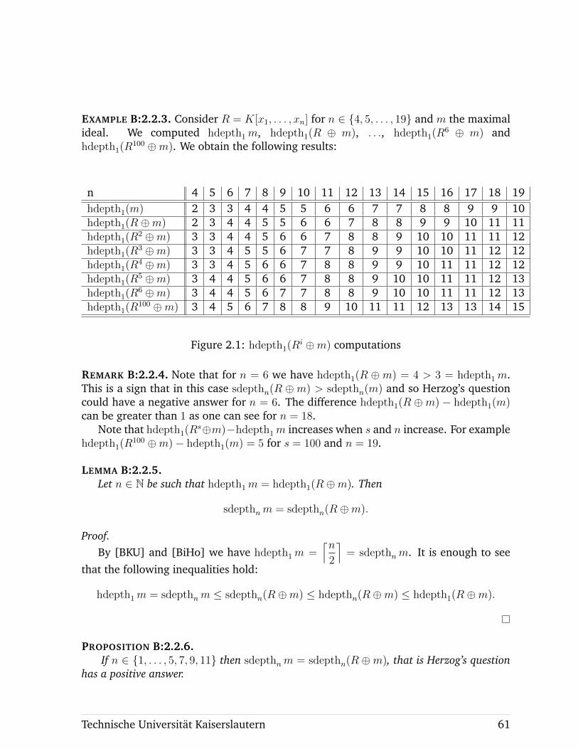
EXAMPLE B:2.2.3. Consider R = K[x1, . . . , xn] for n ∈ {4, 5, . . . , 19} and m the maximalideal. We computed hdepth1m, hdepth1(R ⊕ m), . . ., hdepth1(R
6 ⊕ m) andhdepth1(R
100 ⊕m). We obtain the following results:
n 4 5 6 7 8 9 10 11 12 13 14 15 16 17 18 19hdepth1(m) 2 3 3 4 4 5 5 6 6 7 7 8 8 9 9 10hdepth1(R⊕m) 2 3 4 4 5 5 6 6 7 8 8 9 9 10 11 11hdepth1(R
2 ⊕m) 3 3 4 4 5 6 6 7 8 8 9 10 10 11 11 12hdepth1(R
3 ⊕m) 3 3 4 5 5 6 7 7 8 9 9 10 10 11 12 12hdepth1(R
4 ⊕m) 3 3 4 5 6 6 7 8 8 9 9 10 11 11 12 12hdepth1(R
5 ⊕m) 3 4 4 5 6 6 7 8 8 9 10 10 11 11 12 13hdepth1(R
6 ⊕m) 3 4 4 5 6 7 7 8 8 9 10 10 11 11 12 13hdepth1(R
100 ⊕m) 3 4 5 6 7 8 8 9 10 11 11 12 13 13 14 15
Figure 2.1: hdepth1(Ri ⊕m) computations
REMARK B:2.2.4. Note that for n = 6 we have hdepth1(R ⊕m) = 4 > 3 = hdepth1m.This is a sign that in this case sdepthn(R ⊕m) > sdepthn(m) and so Herzog’s questioncould have a negative answer for n = 6. The difference hdepth1(R ⊕m) − hdepth1(m)can be greater than 1 as one can see for n = 18.
Note that hdepth1(Rs⊕m)−hdepth1m increases when s and n increase. For example
hdepth1(R100 ⊕m)− hdepth1(m) = 5 for s = 100 and n = 19.
LEMMA B:2.2.5.Let n ∈ N be such that hdepth1m = hdepth1(R⊕m). Then
sdepthnm = sdepthn(R⊕m).
Proof.By [BKU] and [BiHo] we have hdepth1m =
⌈n2
⌉= sdepthnm. It is enough to see
that the following inequalities hold:
hdepth1m = sdepthnm ≤ sdepthn(R⊕m) ≤ hdepthn(R⊕m) ≤ hdepth1(R⊕m).
PROPOSITION B:2.2.6.If n ∈ {1, . . . , 5, 7, 9, 11} then sdepthnm = sdepthn(R ⊕m), that is Herzog’s question
has a positive answer.
Technische Universitat Kaiserslautern 61
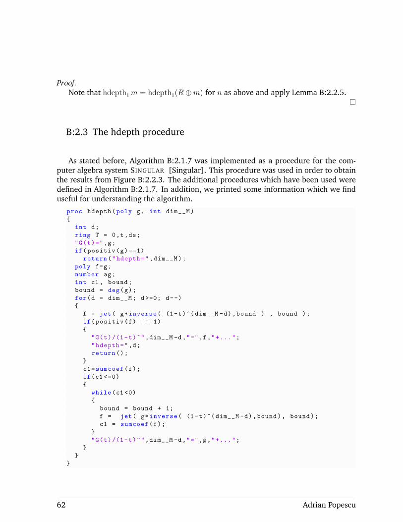
Proof.Note that hdepth1m = hdepth1(R⊕m) for n as above and apply Lemma B:2.2.5.
B:2.3 The hdepth procedure
As stated before, Algorithm B:2.1.7 was implemented as a procedure for the com-puter algebra system SINGULAR [Singular]. This procedure was used in order to obtainthe results from Figure B:2.2.3. The additional procedures which have been used weredefined in Algorithm B:2.1.7. In addition, we printed some information which we finduseful for understanding the algorithm.
proc hdepth(poly g, int dim__M)
{
int d;
ring T = 0,t,ds;
"G(t)=",g;
if(positiv(g)==1)
return("hdepth=",dim__M);
poly f=g;
number ag;
int c1 , bound;
bound = deg(g);
for(d = dim__M; d>=0; d--)
{
f = jet( g*inverse( (1-t)^(dim__M -d),bound ) , bound );
if(positiv(f) == 1)
{
"G(t)/(1-t)^",dim__M -d,"=",f,"+...";
"hdepth=",d;
return ();
}
c1=sumcoef(f);
if(c1 <=0)
{
while(c1 <0)
{
bound = bound + 1;
f = jet( g*inverse( (1-t)^(dim__M -d),bound), bound);
c1 = sumcoef(f);
}
"G(t)/(1-t)^",dim__M -d,"=",g,"+...";
}
}
}
62 Adrian Popescu
CHAPTER B:3
THE STANLEY CONJECTURE
B:3.1 The present stay of Stanley’s Conjecture and its impact in Com-mutative Algebra
For more than 30 years the Stanley Conjecture was a dream for many people workingin combinatorics and commutative algebra. Many people believed that this conjectureholds and tried to prove directly some of its consequences. For example in this way alower bound of depth given by Lyubeznik [Ly] was extended by Herzog et al. [HPV] forsdepth.
Some numerical upper bounds of sdepth give also upper bounds of depth, which areindependent of char K. More precisely, let S = K[x1, . . . , xn], n ∈ N, be a polynomialring over a field K and I ) J two squarefree monomial ideals of S. Then denote byρj(I \ J) for the number of all squarefree monomials of degrees j in I \ J .
THEOREM B:3.1.1([DP6, Theorem 1.3]
).
Assume that depthS(I/J) ≥ t, where t ∈ Z such that d ≤ t < n. If
ρt+1(I \ J) < αt :=t−d∑i=0
(−1)t−d+iρd+i(I \ J), then depthS(I/J) = t independently of
the characteristic of K.
An extension is given below.
THEOREM B:3.1.2(Shen [Sh, Theorem 2.4]
).
Assume that depthS(I/J) ≥ t, where t is an integer such that d ≤ t < n. If for some
k with d + 1 ≤ k ≤ t + 1 it holds ρk(I \ J) <k−1∑j=d
(−1)k−j+1
(t+ 1− jk − j
)ρj(I \ J), then
depthS(I/J) = t independently of the characteristic of K.
Shen’s proof is very short, based on a strong tool, namely the Hilbert depth consid-ered by Bruns-Krattenhaler-Uliczka [BKU] (see also [Uli], [IM]) that was introduced inSection B:2.1.
Let r be the number of the squarefree monomials of degrees d of I and B (resp. C)be the set of the squarefree monomials of degrees d+1 (resp. d+2) of I \J . Set s = |B|,
Technische Universitat Kaiserslautern 63
q = |C|. Theorems B:3.1.1 and B:3.1.2 lead to the following:
THEOREM B:3.1.3(D. Popescu, [DP2]
).
If s > q + r then depthS I/J ≤ d+ 1.
THEOREM B:3.1.4(Shen, [Sh]
).
If s < 2r then depthS I/J ≤ d+ 1.
If r > s then Theorem B:3.1.1 says that depthS I/J = d, namely the minimumpossible.
THEOREM B:3.1.5(D. Popescu, [DP5, Theorem 4.3]
).
If sdepthS I/J = d, then depthS I/J = d, that is Stanley’s Conjecture holds in thiscase.
The next step in proving Stanley’s Conjecture is the following weaker case.
CONJECTURE B:3.1.6.Suppose that I ⊂ S is minimally generated by some squarefree monomials f1, . . . , fk of
degrees d, and a set H of squarefree monomials of degrees ≥ d+ 1. If sdepthS I/J = d+ 1,then depthS I/J ≤ d+ 1.
A partial answer is the following theorem which is the subject of Section B:3.3.
THEOREM B:3.1.7(A. Popescu and D. Popescu [APDP1, Theorem 0.6]
).
Let C be the set of the squarefree monomials of degree d+2 of I \J . Conjecture B:3.1.6holds in each of the following two cases:
1. r ≤ 3,
2. r = 4, E = ∅ and there exists c ∈ C such that supp c 6⊂4⋃i=1
supp fi.
However, Conjecture B:3.1.6 is false in general as shows an example similar to theone given in [DuGo].
EXAMPLE B:3.1.8 (Stanley Conjecture Counterexample). Let n = 6, r = 5, E = ∅,I = (yt, yz, xy, xu, xv) ⊂ K[x, y, z, t, u, v], J = (ytv, xtv, yzv, xtu). Then
sdepthS I/J < depthS I/J.
We should point out that the examples from [DuGo] do not say that Stanley’s Conjec-ture is false in the frame of ideals. On the other hand, as we saw, there exist many casesin which Stanley’s Conjecture holds. We should mention also that Katthan proved in
64 Adrian Popescu
[Ka] that if J is an ideal (not necessarily squarefree) generated by at most 6 generatorsthen Stanley’s Conjecture holds for S/J .
Why is important to know the cases when Stanley’s Conjecture holds? We recall that ifthis is the case for the Stanley-Reisner of a certain simplicial complex then this is par-titionable (see [HSY]). Another reason is explained in [BIS]. More precisely, the com-puter algebra system NORMALIZ uses Stanley decompositions to compute the Hilbertseries. Thus if Stanley’s Conjecture holds, then we have an idea about how “good”could this decomposition be, i.e. how big could its sdepth be. We should recall thathere we speak about multigraded Stanley’s Conjecture which sometime could fail, butthe graded Stanley’s Conjecture always holds (see [BKU, Theorem 2.5]). The fact thatmultigraded Stanley’s Conjecture fails sometimes implies that it is harder to find thebest existing multigraded Stanley decomposition in order to compute the multigradedHilbert series.
B:3.2 The Stanley Conjecture on intersections of three monomial primeideals.
This section contains results published in [AP1]. These ideas were often used in pa-pers like [HPV], [RTU] and [Ta]. Let S = K[x1, . . . , xn], I be an ideal inK[x1, . . . , xr] = S ′ and J be an ideal in K[xr+1, . . . , xn] = S ′′, where 1 < r < n. Thefollowing two lemmas are elementary, their proofs being suggested by [Vi, Theorem2.2.21] and [PQ, Lemma 4.1]. We include these for the sake of our completeness.
LEMMA B:3.2.1.With the notations as above, the following equality holds:
depthS(IS ∩ JS) = depthS′(I) + depthS′′(J).
Proof.Let us consider the following exact sequence of S-modules:
0→ S
IS ∩ JS→ S
IS⊕ S
JS→ S
IS + JS→ 0.
By [Vi, Theorem 2.2.21] it follows that
depthS
(S
IS + JS
)= depthS′
(S ′
I
)+ depthS′′
(S ′′
J
).
But since depth(S/IS) = depthS′(S′/I) + (n − r) and depth(S/JS) = depthS′′(S
′′/J) +
r, we obtain depth
(S
IS⊕ S
JS
)> depth
(S
IS + JS
). Applying Depth Lemma to the
Technische Universitat Kaiserslautern 65
above exact sequence yields
depthS
(S
IS ∩ JS
)= depthS
(S
IS + JS
)+ 1 = depthS′
(S ′
I
)+ depthS′′
(S ′′
J
)+ 1.
We are done since
depthS (IS ∩ JS) = depthS
(S
IS + JS
)+ 2 = depthS′(I) + depthS′′(J).
The following result is analogous to [Ra, Theorem 3.1].
LEMMA B:3.2.2.With the notations from the previous lemma, the following inequality yields:
sdepthS(IS ∩ JS) ≥ sdepthS′(I) + sdepthS′′(J).
Proof.Let M(I) be the monomials from the ideal I and consider two polynomials
f ∈ M(I) and g ∈ M(J). The correspondence (f, g) 7→ f · g defines an injective mapϕ :M(I)×M(J)→M(IS ∩ JS). If w ∈ M(IS ∩ JS), then w = f · g for some mono-mials f ∈ S ′ and g ∈ S ′′; hence f · g ∈ IS, therefore f ∈ IS ∩ S ′ = I since the variablesof g are free over S/IS. Similarly we obtain g ∈ J , and so ϕ becomes surjective sincew = ϕ(f, g).
Let D′ be a Stanley decomposition of I,
D′ : I =s⊕i=1
uiK[Zi],
with sdepthS′(D′) = sdepthS′(I), and let D′′ be a Stanley decomposition of J
D′′ : J =t⊕
j=1
vjK[Ti],
with sdepthS′′(D′′) = sdepthS′′(J). D′ and D′′ induce a Stanley decomposition overIS ∩ JS because ϕ is bijective:
D : IS ∩ JS =t⊕
j=1
s⊕i=1
uivjK[Zi ∪ Tj].
Therefore,
sdepthS(IS ∩ JS) ≥ sdepthS(D) = mini,j(|Zi|+ |Tj|) ≥ mini |Zi|+ minj |Tj| == sdepthS′(D′) + sdepthS′′(D′′) = sdepthS′(I) + sdepthS′′(J).
66 Adrian Popescu
REMARK B:3.2.3. The inequality of the above lemma can be strict as happens in thecase when n = 4, r = 2, I = (x1, x2), J = (x3, x4). Indeed, then sdepthS′(I) = 1,sdepthS′′(J) = 1, and sdepthS(IS ∩ JS) = 3 > 2 = sdepthS′(I) + sdepthS′′(J), as showsthe Stanley decomposition
IS ∩ JS = x1x3K[x1, x3, x4]⊕ x1x4K[x1, x2, x4]⊕x2x3K[x1, x2, x3]⊕ x2x4K[x2, x3, x4]⊕ x1x2x3x4S.
THEOREM B:3.2.4.Let ri ∈ N such that 0 = r0 < r1 < r2 < . . . < rs = n and S = K[x1, . . . , xn]. Denote
by P1 = (x1, . . . , xr1), P2 = (xr1+1, . . . , xr2), . . . , Ps = (xrs−1+1, . . . , xrs) and I =s⋂i=1
Pi.
Then,sdepth (I) ≥ depth (I) = s.
In particular Stanley’s Conjecture holds in this case.
Proof.
Denote by Si = K[xri−1+1, . . . , xri ]. Since depthSi
(Si
Pi ∩ Si
)= 0 we obtain
depthSi(Pi ∩ Si) = 1. By Lemma B:3.2.1 and recurrence we obtain depth(I) = s. Apply-ing Lemma B:3.2.2, by recurrence and [Sh] it results that
sdepthS (I) ≥s∑i=1
sdepthSi(Pi ∩ Si) =s∑i=1
⌈ri − ri−1
2
⌉≥ s,
where dae is the lowest integer number greater or equal to a ∈ R.
REMARK B:3.2.5. If s = 2, then Ishaq [Is, Corollary 2.9, 2.10] proved that
sdepth(I) =
⌈n+ 1
2
⌉if either n is odd, or n is even but r1 is odd, and
n
2≤ sdepth(I) ≤ n
2+ 1 if n and r1 are even.
We need the following two lemmas:
LEMMA B:3.2.6([PQ, Lemma 4.3]
).
Let S = K[x1, . . . , xn] and consider the ideals Q = (x1, . . . , xt) and Q′ = (xr+1, . . . , xn)where 1 ≤ r ≤ t < n. Then
sdepth(Q ∩Q′) ≥⌈r
2
⌉+
⌈n− t
2
⌉.
LEMMA B:3.2.7([HVZ, Lemma 3.6]
).
Let I ⊂ S = K[x1, . . . , xn] be an ideal and S ′ = S[xn+1, . . . , xt], where t > n. Then,
sdepthS′(IS′) = sdepthS(I) + (t− n).
Technische Universitat Kaiserslautern 67
PROPOSITION B:3.2.8.Let P1,P2,P3 be three non-zero monomial prime ideals of S not included one in the
other such that3∑i=1
Pi = (x1, . . . , xn). Let I=P1 ∩ P2 ∩ P3.. Then
depth (I) =
{3, if Pi 6⊂ Pj + Pk for any different i, j, k ∈ {1, 2, 3}n+ 2−max{ht(Pi + Pj), ht(Pi + Pk)}, if Pi ⊂ Pj + Pk .
Proof.Consider the following exact sequence of S-modules:
0→ S
P1 ∩ P2
→ S
P1
⊕ S
P2
→ S
P1 + P2
→ 0. (B:3.1)
We have
depth
(S
P1 + P2
)= n− ht(P1 + P2)
and
depth
(S
P1
⊕ S
P2
)= min
{depth
(S
P1
), depth
(S
P2
)}= n−max {ht(P1), ht(P2)} .
By hypotheses we know that ht(P1 + P2) > max{ht(P1), ht(P2)} and hencen− ht(P1 + P2) < n−max{ht(P1), ht(P2)}. This leads to depth( S
P1+P2) < depth( S
P1⊕ S
P2)
and by applying Depth Lemma to B:3.1 we obtain
depth(S
P1 ∩ P2
) = n− ht(P1 + P2) + 1.
There are two cases:Case 1: Pi 6⊂ Pj + Pk for any different i, j, k ∈ {1, 2, 3}.
Let us consider the following two exact sequences of S-modules:
0→ S
I→ S
P1 ∩ P2
⊕ S
P3
→ S
P3 + (P1 ∩ P2)→ 0, (B:3.2)
0→ S
(P1 + P3) ∩ (P2 + P3)→ S
(P1 + P3)⊕ S
(P2 + P3)→ S
P1 + P2 + P3
→ 0. (B:3.3)
By the hypothesis of this case, we have depth( SP1+P3
) > 0 and depth( SP2+P3
) > 0. Ap-
plying Depth Lemma to (B:3.3) we obtain depth
(S
(P1 + P3) ∩ (P2 + P3)
)= 1 because
P1 + P2 + P3 is the maximal ideal. But (P1 + P3)∩ (P2 + P3) = P3 + (P1 ∩ P2) and there-
fore depth
(S
P3 + (P1 ∩ P2)
)= 1. Using again the hypothesis of this case in (B:3.2) we
can say that depth
(S
P3
)> 1 and depth
(S
P1 ∩ P2
)> 1. By Depth Lemma applied to
68 Adrian Popescu
(B:3.2) we have depth(S/I) = 2. Thus depth (I) = 3.Case 2: There exist different i, j, k ∈ {1, 2, 3} such that Pi ⊂ Pj + Pk.
After a possible renumbering of (Pi)1≤i≤3 we may suppose that P1 ⊂ P2 + P3. Notethat P1 = P1 ∩ P2 + P1 ∩ P3. Consider the next exact sequence of S-modules:
0→ S
I→ S
(P1 ∩ P2)⊕ S
P1 ∩ P3
→ S
P1
→ 0. (B:3.4)
Note that depth
(S
P1 ∩ P2
)and depth
(S
P1 ∩ P3
)are smaller or equal than dim
(S
P1
)(see [BH]). We prove that
depth
(S
I
)= min
{depth
(S
P1 ∩ P2
), depth
(S
P1 ∩ P3
)}.
If
dim
(S
P1
)> min
{depth
(S
P1 ∩ P2
), depth
(S
P1 ∩ P3
)}n− ht(P1) n+ 1−max {ht(P1 + P2), ht(P1 + P3)}
then we are done by Depth Lemma applied to (B:3.4).Otherwise, n−ht(P1) = n+1−max{ht(P1+P2), ht(P1+P3)} and applying again Depth
Lemma we obtain that depth(SI
)≥ min
{depth
(S
P1∩P2
), depth
(S
P1∩P3
)}, the inequality
being equality since
depth
(S
I
)≤ dim
(S
P1
)= n− ht(P1) = min
{depth
(S
P1 ∩ P2
), depth
(S
P1 ∩ P3
)}.
Thus we have proved that
depth(S/I) = n+ 1−max{ht(P1 + P2), ht(P1 + P3)}
and sodepth (I) = n+ 2−max{ht(P1 + P2), ht(P1 + P3)}.
The next lemma presents a decomposition of the above I as a direct sum of its linearsubspaces. These subspaces are “simpler” monomial ideals, for which we already know“good” Stanley decompositions. Substituting them in the above direct sum we get somespecial Stanley decompositions where it is easier to lower bound their Stanley depth.
We may suppose after a possible renumbering of variables that P1 = (x1, . . . , xr). Letus denote the following:
Technische Universitat Kaiserslautern 69
b2 − the number of variables from {xi|1 ≤ i ≤ r} for which xi ∈ P2,b3 − the number of variables from {xi|1 ≤ i ≤ r} for which xi ∈ P3,b1 − the number of variables from {xi|1 ≤ i ≤ r} for which xi ∈ P2 ∪ P3,a23 − the number of variables from {xi|1 ≤ i ≤ r} for which xi ∈ P2 \ P3,a32 − the number of variables from {xi|1 ≤ i ≤ r} for which xi ∈ P3 \ P2,c − the number of variables from {xi|r + 1 ≤ i ≤ n} for which xi ∈ P2 ∩ P3,
A =⌈a32
2
⌉+
⌈ht(P2)− b2
2
⌉+ n− a32 − ht(P2),
B =⌈a23
2
⌉+
⌈ht(P3)− b3
2
⌉+ n− a23 − ht(P3),
C =
⌈r − b1
2
⌉+
⌈ht(P2)− b2 − c
2
⌉+
⌈ht(P3)− b3 − c
2
⌉,
S ′ = K[{xi|1 ≤ i ≤ r, xi 6∈ P3}
],
S ′′ = K[{xi|1 ≤ i ≤ r, xi 6∈ P2}
],
S = K[{xi|1 ≤ i ≤ r, xi 6∈ P2 + P3}, xr+1, . . . , xn
].
LEMMA B:3.2.9.Let S = K[x1, . . . , xn], P1,P2,P3 be three non-zero monomial prime ideals not included
one in the other such that3∑i=1
Pi = (x1, . . . , xn) and I = P1 ∩ P2 ∩ P3. The next sum is a
direct sum of linear subspaces of I:
I = I1 ⊕ I2 ⊕ I3 ⊕ I4,
where:
I1 =(I ∩K[x1, . . . , xr]
)S,
I2 = (P2 ∩ S ′)S ′[xr+1, . . . , xn] ∩(P3 ∩ S ′[xr+1, . . . , xn]
),
I3 = (P3 ∩ S ′′)S ′′[xr+1, . . . , xn] ∩(P2 ∩ S ′′[xr+1, . . . , xn]
),
I4 = I ∩ S.
Proof.Note that I ⊇ I1 + I2 + I3 + I4 is obvious because every Ii ⊆ I. Conversely, let a be a
monomial from I. If a 6∈ I1, then we have the next three disjoint cases:Case 1. a 6∈
(P2 ∩K[x1, . . . , xr]
)S but a ∈
(P3 ∩K[x1, . . . , xr]
)S.
Let a = uv, where u ∈ K[x1, . . . , xr] and v ∈ K[xr+1, . . . , xn] monomials. From thehypothesis of this case we get that u 6∈
(P2 ∩K[x1, . . . , xr]
). But P2 is a prime ideal, so
it follows that v ∈ P2, which leads us to a ∈ I3.
70 Adrian Popescu
Case 2. a ∈(P2 ∩K[x1, . . . , xr]
)S but a 6∈
(P3 ∩K[x1, . . . , xr]
)S.
This case is similar with Case 1.Case 3. a 6∈
(P2 ∩K[x1, . . . , xr]
)S and a 6∈
(P3 ∩K[x1, . . . , xr]
)S.
Let a = uv, where u ∈ K[x1, . . . , xr] and v ∈ K[xr+1, . . . , xn] monomials. From thehypothesis of this case we get that u 6∈ P2 ∩ K[x1, . . . , xr] and u 6∈ P3 ∩ K[x1, . . . , xr].Thus v ∈ P2 ∩ P3 ∩ K[xr+1, . . . , xn] because P2 and P3 are prime ideals. Hence a ∈ I4since u ∈ P1.
Because the cases are disjoint we have obtained that the sum I = I1 + I2 + I3 + I4 isdirect.
PROPOSITION B:3.2.10.Let P1, P2, P3 be three non-zero prime monomial ideals of S such that there exists no
inclusion between any two of them,3∑i=1
Pi = (x1, . . . , xn) and set I = P1 ∩ P2 ∩ P3. With
the above notations we have:
sdepth (I) ≥{
min{A,B,C}, if Pi 6⊂ Pj + Pk for any different i, j, k ∈ {1, 2, 3}min{A,B}, if P1 ⊂ P2 + P3.
The proof follows from Lemma B:3.2.9, but first we explain the idea in the followingexample:
EXAMPLE B:3.2.11. Let S = K[x1, x2, x3, x4] , P1 = (x1, x2), P2 = (x2, x3, x4) andP3 = (x1, x3). Then I = P1 ∩P2 ∩P3 = (x1x2, x1x3, x1x4, x2x3) and the following Stanleydecomposition of I is given by Lemma B:3.2.9:
I = (x1x2) K[x1, x2, x3, x4]⊕ (x2x3) K[x2, x3, x4]⊕ (x1x3, x1x4) K[x1, x3, x4].
Note that the last term of Lemma B:3.2.9 does not appear in this example sinceP1 ⊂ P2 + P3. We see that the first and the third term in the sum are principal ide-als. Therefore sdepth
((x1x2)K[x1, x2, x3, x4]
)= 4 and sdepth
((x2x3)K[x2, x3, x4]
)= 3.
As for the third term we use Lemma B:3.2.6, so
sdepth((x1) ∩ (x3, x4) K[x1, x3, x4]
)=
⌈1
2
⌉+
⌈2
2
⌉= 2.
Thus sdepth (I) ≥ min{4, 2, 3} = 2. The same statement follows fromProposition B:3.2.10 because in this case b2 = 1, b3 = 1, b1 = 2, a23 = 1, a32 = 1,c = 1, A = 2 and B = 3. Therefore sdepth(I) ≥ min{A,B} = 2. Note that depth (I) = 2by Proposition B:3.2.8. Therefore Stanley’s Conjecture holds for this example.
Technische Universitat Kaiserslautern 71
Proof of Proposition B:3.2.10.From Lemma B:3.2.9 we have the direct sum of spaces I = I1 ⊕ I2 ⊕ I3 ⊕ I4 where:
I1 =(I ∩K[x1, . . . , xr]
)S,
I2 = (P2 ∩ S ′)S ′[xr+1, . . . , xn] ∩(P3 ∩ S ′[xr+1, . . . , xn]
),
I3 = (P3 ∩ S ′′)S ′′[xr+1, . . . , xn] ∩(P2 ∩ S ′′[xr+1, . . . , xn]
),
I4 = I ∩ S.
Then sdepth (I) ≥ min1≤i≤4
sdepth(Ii). Note that sdepthS (I1) is greater or equal than
the number of free variables which is n− r = dim(S/P1) ≥ sdepth (I) by [Artin1] (so I1can be always omitted for sdepth computation). By Lemma B:3.2.2 we have
sdepthS′[xr+1,...,xn] (I2) ≥ sdepthS′(P2 ∩ S ′) + sdepthK[xr+1,...,xn]
(P3 ∩K[xr+1, . . . , xn]
)=
=(⌈
a232
⌉+ r − b3 − a23
)+(⌈
ht(P3)−b32
⌉+ (n− r)− (ht(P3)− b3)
)=⌈a23
2
⌉+
⌈ht(P3)− b3
2
⌉+ n− a23 − ht(P3) =
= B,
by also applying [Sh](see [Ci]). Similarly we get
sdepthS′′[xr+1,...,xn] (I3) ≥⌈a32
2
⌉+
⌈ht(P2)− b2
2
⌉+ n− a32 − ht(P2) = A.
Finally,
sdepthS (I4) ≥⌈r − b1
2
⌉+ sdepthK[xr+1,...,xn]
(P2 ∩ P3 ∩K[xr+1, . . . , xn]
).
There are two cases:Case 1. If Pi 6⊂ Pj + Pk for any different i, j, k ∈ {1, 2, 3}Note that P2 ∩ K[xr+1, . . . , xn] 6⊂ P3 ∩ K[xr+1, . . . , xn] (otherwise it would result
that P2 ⊂ P1 + P3, contradicting the hypothesis of this case). In the same idea P3 ∩K[xr+1, . . . , xn] 6⊂ P2∩K[xr+1, . . . , xn]. By applying Lemma B:3.2.6 for r = ht(P2)−b2−cand n− t = ht(P3)− b3 − c we get
sdepthK[xr+1,...,xn]
(P2 ∩ P3 ∩K[xr+1, . . . , xn]
)≥⌈
ht(P2)− b2 − c2
⌉+
⌈ht(P3)− b3 − c
2
⌉.
Note that there are no free variables above. Therefore
sdepthS (I4) ≥⌈r − b1
2
⌉+
⌈ht(P2)− b2 − c
2
⌉+
⌈ht(P3)− b3 − c
2
⌉= C.
Consequently, it followssdepth (I) ≥ min{A,B,C}.
72 Adrian Popescu
Case 2. If P1 ⊂ P2 + P3
Note that in this case S = K[xr+1, . . . , xn] and P1∩ S = 0. Thus I4 does not appear inthe Stanley decomposition of I given by Lemma B:3.2.9. Hence sdepth (I) ≥ min{A,B}.
If one Ii = 0, we consider in both cases that its corresponding integer from {A,B,C}will not appear in the sdepth formula.
REMARK B:3.2.12. In the notations and hypotheses of Proposition B:3.2.10, letS = S[xn+1, . . . , xt] for some t > n. Then
sdepthS (IS) ≥{
min{A,B,C}+ (t− n), if Pi 6⊂ Pj + Pk for any different i, j, kmin{A,B}+ (t− n), if P1 ⊂ P2 + P3,
by the Lemma B:3.2.7 and the Proposition B:3.2.10.
THEOREM B:3.2.13.Let P1, P2 and P3 be three non-zero prime monomial ideals of S not included one in
the other and set I = P1 ∩ P2 ∩ P3. Then,
sdepth (I) ≥ depth (I).
Proof.
By [HVZ] it is enough to suppose the case when3∑i=1
Pi = (x1, . . . , xn). As in
Proposition B:3.2.8 and Proposition B:3.2.10 there are two cases:Case 1. If Pi 6⊂ Pj + Pk for any different i, j, k ∈ {1, 2, 3}.By Propositions B:3.2.8 and B:3.2.10 we have depth(I) = 3 and
sdepth (I) ≥ min{A,B,C}. We have to prove that A ≥ 3, B ≥ 3 and C ≥ 3.By hypothesis of Case 1 we have n ≥ 3 and A ≥ d1
2e+ d1
2e+ 1 = 3. Similarly we get
B ≥ 3. Also it follows C ≥ d12e+ d1
2e+ d1
2e = 3. Therefore, sdepth (I) ≥ depth(I).
Case 2. There exist different 1 ≤ i ≤ j ≤ k ≤ 3 such that Pi ⊂ Pj + Pk.After a possible renumbering of (Pi)1≤i≤3 we may suppose that P1 ⊂ P2 + P3. In this
case depth(I) = n + 2 −max{ht(P1 + P2), ht(P1 + P3)} and sdepth (I) ≥ min{A,B} byPropositions B:3.2.8 and B:3.2.10. Since P1 ⊂ P2 + P3 we have
a32 + ht(P2) = ht(P1 + P2).
As the Pi’s are not included one in the other we get⌈a322
⌉+
⌈ht(P2)− b2
2
⌉+ n− (a32 + ht(P2)) ≥ 1 + 1 + n− ht(P1 + P2),
thus A ≥ depth(I). Similarly it will result that B ≥ depth(I).In conclusion we proved that
sdepth (I) ≥ depth (I).
Technische Universitat Kaiserslautern 73
Next we express the integers A, B, C only in terms of heights of Pi, thus indepen-dently of the numbering of the variables.
PROPOSITION B:3.2.14.With the notations above, the following holds:
A =
⌈3n− ht(P1 + P2)− ht(P2 + P3)− ht(P2)
2
⌉+
⌈ht(P1 + P2)− ht(P1)
2
⌉,
B =
⌈3n− ht(P1 + P3)− ht(P2 + P3)− ht(P3)
2
⌉+
⌈ht(P1 + P3)− ht(P1)
2
⌉,
C =
⌈n− ht(P2 + P3)
2
⌉+
⌈n− ht(P1 + P3)
2
⌉+
⌈n− ht(P1 + P2)
2
⌉.
Proof.By definition we have
r = ht(P1),b2 = ht(P1) + ht(P2)− ht(P1 + P2),b3 = ht(P1) + ht(P3)− ht(P1 + P3),b1 = ht(P1) + ht(P2 + P3)− n,a23 = ht(P1 + P3) + ht(P2 + P3)− ht(P3)− n,a32 = ht(P1 + P2) + ht(P2 + P3)− ht(P2)− n,c = ht(P1 + P2) + ht(P1 + P3)− ht(P1)− n,
and it is enough to replace them into the definition of A,B and C.
B:3.3 The Stanley Conjecture for factors of monomial ideals
The results of this section are published in [APDP1].Let I ) J be two squarefree monomial ideals of S. We assume that I is generated
by squarefree monomials f1, . . . , fr of degrees d for some d ∈ N and a set of squarefreemonomials E of degree ≥ d + 1. We may suppose that either J = 0, or is generatedby some squarefree monomials of degrees ≥ d + 1. B (resp. C) denotes the set of thesquarefree monomials of degrees d+ 1 (resp. d+ 2) of I \ J .
LEMMA B:3.3.1.Let J ⊂ I be square free monomial ideals and j ∈ [n] be such that (J : xj) 6= (I : xj).
Then depthS(I : xj)
(J : xj)≥ depthS
I
J.
74 Adrian Popescu
Proof.We have
pdSI
J≥ pdSxj
(I
J
)⊗ Sxj = pdSxj
((I : xj)
(J : xj)
)⊗ Sxj = pdS
((I : xj)
(J : xj)
)the last equality holds since xj does not appear among the generators of (I : xj) and(J : xj). Now it is enough to apply the Auslander-Buchsbaum Theorem.
LEMMA B:3.3.2.Let t ∈ [n]. Suppose that I 6= J + I ∩ (xt) and depthS
I
J + I ∩ (xt)= d. If
depthS I/J ≥ d+ 1 then depthS I/J = d+ 1.
Proof.In the following exact sequence
0 −→ I : xtJ : xt
xt−−−→ I
J−→ I
J + I ∩ (xt)−→ 0
the first term has depth d+1 by the Depth Lemma. We are done by applying the previouslemma.
Let wij be the least common multiple of fi and fj and set W to be the set of allwij ∈ B.
LEMMA B:3.3.3.If d = 1 and B ⊂ E ∪W then depthS I/J = 1.
Proof.First suppose that E = ∅ and assume that I = (x1, . . . , xr). Set S ′ = K[x1, . . . , xr],
I ′ = I ∩ S ′, J ′ = J ∩ S ′. By hypothesis B ⊂ S ′ and it follows that (xr+1, . . . , xn)I ⊂ J ,leading to the equality depthS I = depthS′ I
′ = 1. But depthS J ≥ 2, if J 6= 0, and sodepthS I/J = 1 by the Depth Lemma.
Now, suppose that E 6= ∅. In the following exact sequence
0 −→ (x1, . . . , xr)
J ∩ (x1, . . . , xr)−→ I
J−→ I
(J, x1, . . . , xr)−→ 0
the first term has depth 1 as above and the last term has depth ≥ d + 1 since it isgenerated by squarefree monomials of degrees ≥ 2 from E. Again the Depth Lemmagives depthS I/J = 1.
LEMMA B:3.3.4.Suppose that I ⊂ S is generated by some squarefree monomials f1, ...fr of degree
d. Assume that for all b ∈ B all divisors of b of degree d are among {f1, . . . , fr}. ThendepthS I/J = d.
Technische Universitat Kaiserslautern 75
Proof.We prove by induction on d ≥ 1. If d = 1 then apply the previous lemma. Assume
that d > 1. We may suppose that n ∈ supp f1. (I : xn) is an extension of a squarefreemonomial ideal I ′ of S ′ = K[x1, . . . , xn−1] which is generated in degree≥ d−1. Similarly(J : xn) is generated by a squarefree monomial ideal J ′ of S ′. Note that the generators ofI ′ of degree d− 1 have the form f ′i = fi/xn for fi ∈ (xn), and the squarefree monomialsB′ of degrees d from I ′ \ J ′ have the form b′ = b/xn for some b ∈ (B ∩ (xn)). Certainlywe must consider also the case when fj 6∈ (xn). If xnfj ∈ J then fj ∈ (J : xn) is notin B′. Otherwise, fj = (xnfj)/xn ∈ B′. Note that all divisors of degree d − 1 of eachb′ ∈ B′ are among f ′i . By induction hypothesis we have depthS′ I
′/J ′ = d − 1 and sodepthS(I : xn)/(J : xn) = d. Now it is enough to apply Lemma B:3.3.1.
An obstruction to improve Lemma B:3.3.3 and the above lemma is given by thefollowing example.
EXAMPLE B:3.3.5. Let n = 5, d = 2, r = 5, I = (x1x2, x1x3, x2x3, x1x4, x3x5),J = (x1x2x5, x1x4x5, x2x3x4, x3x4x5) and B = {x1x2x3, x1x2x4, x1x3x4, x1x3x5, x2x3x5}.We have depthS I/J = 3 because depthS S/J = 3, depthS S/I = 2 and with the help ofDepth Lemma. Note that each b ∈ B is the least common multiple of two generators ofI, but for example b = x1x2x4 has x2x4 6∈ I as a divisor of degree 2.
Let C3 be the set of all c ∈ C having all divisors from B \E in W . In particular eachmonomial of C3 is the least common multiple of three of fi. The converse is not true asshows the following example.
EXAMPLE B:3.3.6. Let n = 4, d = 2, r = 3, f1 = x1x2, f2 = x2x3, f3 = x3x4,I = (f1, f2, f3) and J = 0. Then c = x1x2x3x4 is the least common multiple of f1, f2, f3but has a divisor b = x1x2x4 ∈ B which is not the least common multiple of two fi.
The next theorem is the key result of this section; the proof of it will be presentedlater in this chapter. The main reason that this proof works for r ≤ 3 but not for r = 4is that in the first case |C3| ≤ 1 but in the second one we may have |C3| = 4, whichmakes the things harder. However, for r ≥ 5 will appear a new problem since we mayhave B ⊂ W and s ≥ 2r (for example when r = 5, d = 2 we may have s = 10 = 2r).We remind that by Theorem B:3.1.4 we had to check Stanley’s Conjecture only whens ≥ 2r.
THEOREM B:3.3.7.Conjecture B:3.1.6 holds for r ≤ 3, the case r = 1 being given in [PZ].
EXAMPLE B:3.3.8. Let n = 5, f1 = x1x2, f2 = x1x3, f3 = x1x4, a = x2x3x5, E = {a},I = (f1, f2, f3, a), J = (x4a). We have w12 = f1x3, w13 = f1x4, w23 = f2x4. Set c = w12x4,c1 = w12x5, c2 = w23x5, c3 = w13x5. Then C = {c, c1, c2, c3} and B \ E = B ∩ (∪i[fi, ci]).
76 Adrian Popescu
Thus s = 7, q = 4, r = 3. It is easy to see that sdepthS I/J = 3. Indeed, note thatc1 is the only c′ ∈ C which is multiple of a. Suppose that there exists a partition P onPI/J with sdepth 4. Then we have necessarily in P the interval [a, c1]. If P contains theinterval [f1, c] then it must contain also the intervals [f2, c2] and so [f3, c3], but then w13 ∈[f1, c] ∩ [f3, c3], that is the union is not disjoint. If P contains the interval [f1, c3] thenP contains either [f3, c], [f2, c2], or [f2, c], [f3, c2], in both cases the intersection of thesetwo intervals contains w23, which is false. By Theorem B:3.3.7 we get depthS I/J ≤ 3,this inequality being in fact an equality.
B:3.4 A special case of r = 4
THEOREM B:3.4.1.Suppose that I ⊂ S is minimally generated by some squarefree monomials {f1, . . . , fr}
of degrees d such that there exists c ∈ C such that supp c 6⊂r⋃i=1
supp fi. If Conjecture
B:3.1.6 holds for r′ < r and sdepthS I/J = d+ 1, then depthS I/J ≤ d+ 1.
Proof.By [PZ, Lemma 2.1] we may assume that C ⊂ (W ). By hypothesis, choose t ∈ supp c
such that t 6∈ ∪i∈[r] supp fi. We may suppose that B ∩ (xt) = {xtf1, . . . xtfe} for somee ≤ r. Set It = I ∩ (xt), Jt = J ∩ (xt) and Ut = It/Jt. Then Bt generates It.
First assume that sdepthS Ut ≤ d + 1. It follows that depthS Ut ≤ d + 1 by [DP2,Theorem 4.3]. But Ut ∼= (I : xt)/(J : xt) and so depthS Ut ≥ depthS I/J by LemmaB:3.3.1, which is enough.
Now assume that Ut has sdepth ≥ d+1. Let PUt be a partition on Ut with sdepth d+2and let [bi, ci] be the disjoint intervals starting with bi = xtfi, i ∈ [e]. We have ci = xtwikifor some 1 ≤ ki ≤ r, ki 6= i because C ⊂ (W ). Note that xtfki ∈ B and so ki ≤ e. Weconsider the intervals [fi, ci]. These intervals contain xtfi and wiki. If wiki = wjkj fori 6= j then we get ci = cj which is false. Thus these intervals are disjoint.
Let Ie be the ideal generated by fj for e < j ≤ r and B \ (∪ei=1[fi, ci]). Set Je = Ie ∩ Jand Ue = Ie/Je. Note that ci 6∈ Ie for any i ∈ [e]. In the following exact sequence
0→ Ie/Je → I/J → I/J + Ie → 0
the last term has a partition of sdepth d + 2 given by the intervals [fi, ci] for 1 ≤ i ≤ e.It follows that Ie 6= Je because sdepthS I/J = d + 1. Then sdepthS Ie/Je ≤ d + 1 using[Ra, Lemma 2.2] and so depthS Ie/Je ≤ d+ 1 by Theorem B:3.3.7 applied for k < r. Butthe last term of the above sequence has depth > d because xt does not annihilate fi fori ∈ [e]. With the Depth Lemma we get depthS I/J ≤ d+ 1.
EXAMPLE B:3.4.2. Let n = 5, r = 4, f1 = x2x3, f2 = x1x2, f3 = x3x4, f4 = x3x5and J = (x1x2x4x5). We have w12 = x1x2x3, w13 = x2x3x4, w14 = x2x3x5, w34 =
Technische Universitat Kaiserslautern 77
x3x4x5, w23 = x1x2x3x4, w24 = x1x2x3x5, C2 = {w23, w24}, C = C2 ∪ {x1w34, x2x3x4x5},I1 = {x1f3, x1f4, f2} ⊃ J , I4 = {f3, x4f2} ⊃ J and B∩(x1) = {x1f3, x1f4, x4f2, x5f2, w12},B ∩ (x4) = {w13, w14, w34, x4f2, x1f3}. Note that sdepthS U1 ≤ d + 1 = 3, sdepthS U4 ≤ 3because |B ∩ (x1)| = |B ∩ (x4)| = 5 > |C ∩ (x1)| + 1 = |C ∩ (x4)| + 1 = 4. ThusdepthS U1 = depthS U4 ≤ 3 and so we get depthS I/J ≤ 3 using two different t.
THEOREM B:3.4.3.Suppose that I ⊂ S is minimally generated by four squarefree monomials {f1, . . . , f4}
of degrees d such that there exists c ∈ C such that supp c 6⊂4⋃i=1
supp fi.
If sdepthS I/J = d+ 1 then depthS I/J ≤ d+ 1.
Proof.Apply Theorem B:3.4.1, since Conjecture B:3.1.6 holds for r < 4 by Theorem B:3.3.7.
B:3.5 Proof of Theorem B:3.3.7
Suppose that E 6= ∅ and s ≤ q + r. For b = f1xi ∈ B set Ib = (f2, . . . , fr, B \ {b}),Jb = J ∩ Ib. If sdepthS Ib/Jb ≥ d + 2 then let Pb be a partition on Ib/Jb with sdepthd+ 2. We may choose Pb such that each interval starting with a squarefree monomial ofdegree d, d + 1 ends with a monomial of C. In Pb we have some intervals [fk, fkxikxjk ],1 < k ≤ r and for all b′ ∈ [B \ {b, f2xi2 , f2xj2 , . . . , frxir , frxjr}] an interval [b′, cb′ ]. Wedefine h : [[{f2, . . . , fr}∪B] \ {b, f2xi2 , f2xj2 , . . . , frxir , frxjr}]→ C by fk → fkxikxjk andb′ → cb′. Then h is an injection and | Imh| = s− r ≤ q (if s = r+ q then h is a bijection).Let g be the map Imh → [[B ∪ {f2, . . . , fr}] \ {b, f2xi2 , f2xj2 , . . . , frxir , frxjr}] given byfkxikxjk → fk and h(b′) → b′. We may suppose that all intervals of Pb starting with amonomial v of degree ≥ d+ 2 have the form [v, v].
LEMMA B:3.5.1.Suppose that the following conditions hold:
1. r = 2, s ≤ q + 2.
2. C ⊂((f1) ∩ (f2)
)∪((E) ∩ (f1, f2)
)∪
⋃a,a′∈Ea6=a′
(a) ∩ (a′)
,
3. sdepthS Ib/Jb ≥ d+ 2 for b ∈ (f1) \ (f2).
Then either sdepthS I/J ≥ d+2, or there exists a nonzero ideal I ′ ( I generated by a subsetof {f1, f2}∪B such that sdepthS I
′/J ′ ≤ d+ 1 for J ′ = J ∩ I ′ and depthS I/(J, I′) ≥ d+ 1.
78 Adrian Popescu
Proof.Since sdepthS Ib/Jb ≥ d + 2 we consider h, g as above for a partition Pb with sdepth
d + 2 of Ib/Jb. We have an interval [f2, c′2] in Pb. Suppose that B ∩ [f2, c
′2] = {u, u′}. By
Theorem B:3.1.4 s ≥ 4 and so there exists a1 ∈ B \ {b, u, u′} such that c1 = h(a1).By recurrence choose if possible ap+1 to be a divisor from B of cp which is not in{b, u, u′, a1, . . . , ap} and set cp = h(ap), p ≥ 1. This construction ends at step p = eif all divisors from B of ce−1 are in {b, u, u′, a1, . . . , ae−1}. Suppose that av, 1 ≤ v < e− 1divides ce−1. Then changing in Pb the intervals [ak, ck], v ≤ k ≤ e − 1 with the intervals[av, ce−1], [ak+1, ck], v ≤ k ≤ e−2 we see that the new ce−1 is the old ce−2. If this new ce−1has a divisor ae which is not in {b, u, u′, a1, . . . , ae−1} then we continue our procedurewith ce = h(ae) and so on. After several such steps we arrive at step p = t when one ofthe following situations holds:
1. all divisors from B of any cp, 1 ≤ p < t are among {a1, . . . , at−1},
2. ct−1 ∈ (u, u′), all its divisors from B are in {a1, . . . , at−1, u, u′}, all divisors fromB of any cp, 1 ≤ p < t− 1 are among {a1, . . . , at−2}, but no cp, 1 ≤ p < t is in (b),
3. ct−1 ∈ (b), but no cp, 1 ≤ p < t− 1 is in (b).
In the first case, set T = {a1, . . . , at−1}, G = B \ T and I ′1 = (f1, G), I ′2 = (f2, G),I ′12 = (f1, f2, G), I ′′ = (G), J ′1 = I ′1 ∩ J , J ′2 = I ′2 ∩ J , J ′12 = I ′12 ∩ J , J ′′ = I ′′ ∩ J . Note thatI ′′ 6= 0 because b ∈ I ′′. Consider the following exact sequence
0→ I ′12/J′12 → I/J → I/(J, I ′12)→ 0.
If T ∩ (f1, f2) = ∅ then the last term has depth ≥ d + 1 and sdepth ≥ d + 2 using therestriction of Pb to (T ) since h(b) /∈ I ′12 , for all b ∈ T . When the first term has sdepth≥ d+ 2 then by [Ra, Lemma 2.2] the middle term has sdepth ≥ d+ 2 which is enough.
If T ∩ (f1) = ∅, but let us say av ∈ (f2) for some 1 ≤ v < t, then in the followingexact sequence
0→ I ′1/J′1 → I/J → I/(J, I ′1)→ 0
the last term has sdepth ≥ d + 2 since h(b) /∈ I ′1 and we may substitute the interval[av, cv] from the restriction of Pb by [f2, cv], the second monomial from [f2, cv] ∩B beingalso in T . As above we get either sdepthS I/J ≥ d + 2, or sdepthS I
′1/J
′1 ≤ d + 1,
depthS I/(J, I′1) ≥ d + 1. Similarly, we do when T ∩ (f2) = ∅ but let us say av ∈ (f1) for
some 1 ≤ v < t.Now, suppose that av1 ∈ (f1) and av2 ∈ (f2) for some 1 ≤ v1 < t, 1 ≤ v2 < t. We may
assume that one from cv1 , cv2 is not in (w12), let us say cv1 6∈ (w12). Indeed, if w12 6∈ Bthen necessary v1 6= v2, otherwise av1 = av2 = w12 ∈ B. Thus cv1 6= cv2 and so one ofcvi 6∈ (w12). If w12 ∈ B and cv1 = xjw12 for some j 6∈ suppw12, then let us say av1 = xjf1and we have xjf2 = av for some 1 ≤ v < t by our hypothesis 1). If cv ∈ (w12) thencv = cv1, which is false. If av1 = w12 then again we have xjf2 = av, for some 1 ≤ v < tand cv 6∈ (w12) because otherwise cv = cv1. Take v2 = v.
Technische Universitat Kaiserslautern 79
In the following exact sequence
0→ I ′′/J ′′ → I/J → I/(J, I ′′)→ 0
the last term has sdepth ≥ d+ 2 the last term has sdepth ≥ d+ 2 since we may replacethe intervals [av1 , cv1 ], [av2 , cv2 ] of the restriction of Pb to (T ) with the disjoint intervals[f1, cv1 ], [f2, cv2 ]. Also the last term has depth ≥ d+ 2 because in the exact sequence
0→ (f2)/(J, I′′) ∩ (f2)→ I/(J, I ′′)→ I/(J, I ′′, f2)→ 0
the ends terms have depth ≥ d + 1 since cv1 6∈ (f2), otherwise cv1 ∈ (w12), whichis false. As above we get either sdepthS I/J ≥ d + 2, or sdepthS I
′′/J ′′ ≤ d + 1,depthS I/(J, I
′′) ≥ d+ 1.In the second case, note that c′2 6= ct−1 because h is injective. Then suppose that
u|ct−1, but u′ is not a divisor of any cp, 1 ≤ p < t. If at−1 ∈ (f2) then change in Pb theinterval [at−1, ct−1] by [f2, ct−1]. If av, 1 ≤ v < t is the second divisor of ct−1 from B∩(f2),change in Pb the intervals [ap, cp], v ≤ p < t by [av, ct−1], [ap+1, cp], v ≤ p < t − 1 wesee that now av, u divide the new cv. Changing in Pb the intervals [av, cv], [f2, c
′2] with
[f2, cv], [u′, c′2], we may proceed as above using I ′1 and T ′ = T ∪ {u}.In the third case, let ct−1 = bxi. If at−1 = f1xi then changing in Pb the interval
[at−1, ct−1] by [f1, ct−1] we get a partition on I/J with sdepth d+2. If f1xi ∈ {a1, . . . , at−2},let us say f1xi = av, 1 ≤ v < t − 1 then we may replace in Pb the intervals [ak, ck],v ≤ k ≤ t − 1 with the intervals [av, ct−1], [ak+1, ck], v ≤ k ≤ t − 2. Now we see that wehave in Pb the interval [av, cv] and switching it with the interval [f1, cv] we get a partitionwith sdepth ≥ d+ 2 for I/J .
Thus we may assume that f1xi /∈ {a1, ..., at−1}. Suppose that f1xi 6∈ {u, u′}. Thenset at = f1xi, cp = h(ap), p ≥ t and choose ap+1 6∈ {b, u, u′, at, . . . , ap} to be a divisor ofB of cp, p ≥ t. If ap = av for v < t, p > t then again change in Pb the intervals [ak, ck],v ≤ k ≤ p − 1 with the intervals [av, cp−1], [ak+1, ck], v ≤ k ≤ p − 2. We have in Pb aninterval [f1xi, ct−1] and switching it to [f1, ct−1] we get a partition with sdepth ≥ d+2 forI/J . Thus we may suppose that ap+1 6∈ {b, u, u′, a1, . . . , ap}. If the procedure stops at stepp = t1 because all the divisors from B of {ct, . . . ct1−1} are among T1 = {at, . . . , at1−1}then we do as above with T1 instead T .
If let us say f1xi = u′ = w12 and at−1 ∈ (f2) then replace in Pb the intervals [f2, c′2],
[at−1, ct−1] with [f2, ct−1],[u, c′2]. Take for at the former u which is now not in [f2, c′2] and
proceed as above. If f1xi = u′ = w12 but at−1 ∈ (E) then there exists another divisor a ofct−1 from B ∩ (f2) different of w12. If a ∈ [f2, c
′2] then we get h(at−1) = ct−1 = c′2 = h(f2),
which is false. Thus we may set at = a, ct = h(at) and proceed as above. If theprocedure stops at step p = t1 because all the divisors from B of {ct, . . . ct1−1} are amongT1 = {at, . . . , at1−1} then we do as above with T1 instead T . If ct−1 ∈ (u, u′), but no cp,t ≤ p < t1 is in (b), then we proceed as in case 2) taking T ′1 = T1∪{u}, or T ′1 = T1∪{u′}.
If ct1−1 = bxj we continue as above with at1 = f1xj. After several such steps wemust arrive in the case p = tl when all divisors from B of ctl−1 are already amongTl = {atl−1
, . . . , atl−1}, or T ′l = Tl ∪ {u}, or T ′l = Tl ∪ {u′}. Finally, using Tl as T , or T ′l asT ′ above we are done.
80 Adrian Popescu
LEMMA B:3.5.2.Suppose that the following conditions hold:
1. r = 3, s ≤ q + 3,
2. C ⊂
3⋃i,j=1i 6=j
(fi) ∩ (fj)
∪ ((E) ∩ (f1, f2, f3))∪
⋃a,a′∈Ea6=a′
(a) ∩ (a′)
,
3. There exists b ∈ (f1) \ (f2, f3) such that sdepthS Ib/Jb ≥ d+ 2.
Then either sdepthS I/J ≥ d+2, or there exists a nonzero ideal I ′ ( I generated by a subsetof {f1, f2, f3}∪B such that sdepthS I
′/J ′ ≤ d+1 for J ′ = J∩I ′ and depthS I/(J, I′) ≥ d+1.
Proof.Consider h, g as above for a partition Pb with sdepth d + 2 of Ib/Jb which exists by
(3). We have two intervals [f2, c′2], [f3, c
′3]in Pb. Suppose that B ∩ [fi, c
′i] = {ui, u′i},
1 < i ≤ 3 . By Theorem B:3.1.4 s ≥ 6 and there exists a1 ∈ B \ {b, u2, u′2, u3, u′3} suchthat c1 = h(a1). By recurrence choose if possible ap+1 to be a divisor from B of cp whichis not in {b, u2, u′2, u3, u′3, a1, . . . , ap} and set cp = h(ap), p ≥ 1. This construction ends atstep p = e if all divisors from B of ce−1 are in {b, u2, u′2, u3, u′3, a1, . . . , ae−1}. Suppose thatav, 1 ≤ v < e − 1 divides ce−1. Then changing in Pb the intervals [ap, cp], v ≤ p ≤ e − 1with the intervals [av, ce−1], [ap+1, cp], v ≤ p ≤ e − 2 we see that the new ce−1 is the oldce−2. If this new ce−1 has a divisor ae which is not in {b, u2, u′2, u3, u′3, a1, . . . , ae−1} thenwe continue our procedure with ce = h(ae) and so on. After several such steps we arriveat step p = t when one of the following situations holds:
1. all divisors from B of any cp, 1 ≤ p < t are among {a1, . . . , at−1},
2. ct−1 ∈ (u2, u′2, u3, u
′3), all its divisors from B are in {a1, . . . , at−1, u2, u′2, u3, u′3}, all
divisors from B of any cp, 1 ≤ p < t − 1 are among {a1, . . . , at−2}, but no cp,1 ≤ p < t is in (b),
3. ct−1 ∈ (b), but no cp, 1 ≤ p < t− 1 is in (b).
In the first case, set T = {a1, . . . , at−1}, G = B \ T and for k = (k1, . . . , km),1 ≤ k1 < . . . < km ≤ 3, 0 ≤ m ≤ 3 set I ′k = (fk1 , . . . , fkm , G), J ′k = I ′k ∩ J , andI ′0 = (G), J ′0 = I ′0 ∩ J for m = 0. Note that I ′0 6= 0 because b ∈ I ′0. Consider the followingexact sequence
0→ I ′k/J′k → I/J → I/(J, I ′k)→ 0.
If T ∩(f1, f2, f3) = ∅ then the last term of the above exact sequence given for k = (1, 2, 3)has depth ≥ d + 1 and sdepth ≥ d + 2 using the restriction of Pb to (T ) since h(b) /∈ I ′k,for all b ∈ T . When the first term has sdepth ≥ d + 2 then by [Ra, Lemma 2.2] themiddle term has sdepth ≥ d+ 2 which is enough.
Technische Universitat Kaiserslautern 81
Suppose that T ∩ (fki) = ∅ if and only if i ∈ [m], for some 0 ≤ m < 3 and setk = (1, . . . ,m). We show that in the following exact sequence
0→ I ′k/J′k → I/J → I/(J, I ′k)→ 0
the last term has sdepth ≥ d+2. For all m < i ≤ 3 we find cvi ∈ (fi) for some 1 ≤ vi < t.We claim that we may choose vi such that for all i 6= j, m < i, j ≤ 3 we have vi 6= vj andone from cvi , cvj is not in (wij). Indeed, this is trivial for m = 2. Suppose that m < 2.If wij 6∈ B then necessary vi 6= vj, otherwise avi = avj = wij ∈ B. Contradiction! Ifwij ∈ B then suppose that cvi = xzwij. Then we see that there exists 1 ≤ vj < t suchthat avj = xzfj. If cvj ∈ (wij) then we have cvj = xzwij = cvi, which is false. Thuscvj 6∈ (wij).
Therefore in the worst case, that is m = 0, we may choose cv1 6∈ (w12), cv2 6∈ (w23). Ifcv1 ∈ (w13) then we may also choose cv3 6∈ (w13). In the case when cv1 6∈ (w13), chooseany cv3 ∈ (f3). We conclude that the possible intervals [fi, cvi ], i ∈ [3] are disjoint. Nextwe change the intervals [avi , cvi ], m < i ≤ 3 from the restriction of Pb to (T ) by [fi, cvi ],the second monomial from [fi, cvi ] ∩ B being also in T . Set k = (1, 2, 3). Also I/(J, I ′k)has depth ≥ d+ 1 because in the exact sequence
0→ (f3)/(f3) ∩ (J, I ′k)→ I/(J, I ′k)→ I/(J, I ′k, f3)→ 0
the last term has has depth ≥ d + 2 since cv2 6∈ (w23) and if cv1 ∈ (f3) then cv1 ∈(w13) but we may find a b′ ∈ (B ∩ (f1)) \ (f3) and we may proceed as in the proof ofLemma B:3.5.1. As above we get either sdepthS I/J ≥ d + 2, or sdepthS I
′1/J
′1 ≤ d + 1,
depthS I/(J, I′1) ≥ d+ 1.
In the second case, note that c′2, c′3 6= ct−1 because h is injective. Then suppose that
u2|ct−1, but u′2 is not a divisor of any cp, 1 ≤ p < t. Also suppose for a moment thatct−1 6∈ (u3, u
′3). If at−1 ∈ (f2) then change in Pb the interval [at−1, ct−1] by [f2, ct−1]. If av2,
1 ≤ v2 < t is the second divisor of ct−1 from B ∩ (f2), change in Pb the intervals [ap, cp],v2 ≤ p < t by [av2 , ct−1], [ap+1, cp], v2 ≤ p < t− 1 we see that now av2 , u2 divide the newcv2 . Change in Pb the intervals [av2 , cv2 ], [f2, c
′2] with [f2, cv2 ], [u′2, c
′2], we may proceed as
above using I ′k for k = (1), or k = (13) and T ′ = T ∪ {u2}.If ct−1 is a multiple of u2 and u3 then it is a multiple of w23 and we may suppose
u2 = u3 = w23, the other u′2, u′3 cannot divide ct−1. Then ct−1 have other two divisors
from B one av2 from (f2), the other av3 from (f3). If v2 = t − 1 we change as above[at−1, ct−1] by [f2, ct−1]. If v2 < t − 1 change in Pb the intervals [ap, cp], v2 ≤ p < tby [av2 , ct−1], [ap+1, cp], v2 ≤ p < t − 1 and we see that now av2 , w23 divide the newcv2 . Change in Pb the intervals [av2 , cv2 ], [av3 , cv3 ] by [f2, cv2 ], [f3, cv3 ]. Note that thesecond monomial of B ∩ [f3, cv3 ] is also in T . As above we may proceed with I1, andT ′ = T ∪ {w23}.
In the third case, let ct−1 = bxi. If at−1 = f1xi then changing in Pb the interval[at−1, ct−1] by [f1, ct−1] we get a partition on I/J with sdepth d+2. If f1xi ∈ {a1, . . . , at−2},let us say f1xi = av, 1 ≤ v < t − 1 then we may replace in Pb the intervals [ak, ck], v ≤k ≤ t− 1 with the intervals [av, ct−1], [ak+1, ck], v ≤ k ≤ t− 2. Now we see that we have
82 Adrian Popescu
in Pb the interval [av, cv] and switching it with the interval [f1, cv] we get a partition withsdepth ≥ d+ 2 for I/J .
Thus we may assume that f1xi /∈ {a1, ..., at−1}. Suppose that f1xi 6∈ {u2, u′2, u3, u′3}.Then set at = f1xi, cp = h(ap), p ≥ t and choose ap+1 6∈ {b, u2, u′2, u3, u′3, at, . . . , ap} tobe a divisor from B of cp, p ≥ t. If ap = av for v < t, p > t then again change in Pbthe intervals [ak, ck], v ≤ k ≤ p − 1 with the intervals [av, cp−1], [ak+1, ck], v ≤ k ≤ p − 2.We have in Pb an interval [f1xi, ct−1] and switching it to [f1, ct−1] we get a partition withsdepth ≥ d + 2 for I/J . Thus we may suppose that ap+1 6∈ {b, u2, u′2, u3, u′3, a1, . . . , ap}.If the procedure stops at step p = t1 because all the divisors from B of {ct, . . . ct1−1} areamong T1 = {at, . . . , at1−1} then we do as above with T1 instead T .
If let us say f1xi = u′2 = w12 and at−1 ∈ (f2) then replace in Pb the intervals [f2, c′2],
[at−1, ct−1] with [f2, ct−1],[u2, c′2]. Take for at the former u2 which is now not in [f2, c′2]
and proceed as above. If f1xi = u′2 = w12 but at−1 ∈ (f3) then ct−1 is the least commonmultiple of f1, f2, f3. If ct−1 ∈ C3 then b = w13, which is false by (3). Otherwise, ct−1is also the least common multiple of two fi (see Example B:3.3.5), but in this case ithas at least four divisors from B and so we may find one at 6∈ {b, u2, u′2, u3, u′3}. Iff1xi = u′2 = w12 but at−1 ∈ (E) then there exists another divisor a from B∩(f2) differentof w12. If a ∈ [f2, c
′2] (i.e. a = u2) then we get h(at−1) = ct−1 = c′2 = h(f2), which is false.
If a ∈ (f3) we get as above b ∈ (f3), which is again false. Thus h is defined on a and wemay set at = a, ct = h(at) and proceed as above. If the procedure stops at step p = t1because all the divisors from B of {ct, . . . ct1−1} are among T1 = {at, . . . , at1−1} then wedo as above with T1 instead T . If ct−1 ∈ (u2, u
′2), but no cp, t ≤ p < t1 is in (b), then we
proceed as in case 2) taking T ′1 = T1 ∪ {u2}, or T ′1 = T1 ∪ {u′2}.If ct1−1 = bxj we continue as above with at1 = f1xj. After several such steps we
must arrive in the case p = tl when all divisors from B of ctl−1 are already amongTl = {atl−1
, . . . , atl−1}, or T ′l = Tl ∪ {u2}, or T ′l = Tl ∪ {u′2}, or T ′l = Tl ∪ {u3}, orT ′l = Tl ∪ {u′3}. Finally, using Tl as T , or T ′l as T ′ above we are done.
Proof of Theorem B:3.3.7.By Theorem B:3.1.3 we may suppose that s ≤ q+r. Apply induction on |E|. If E = ∅
we may apply [PZ]. Actually, in this case it is enough to apply as below Lemma [PZ,Lemma 2.1]. Suppose that |E| > 0 and B ∩ (f1, . . . , fr) 6= ∅, r = 2, 3, otherwise we getdepthS I/J ≤ d + 1. Moreover, we see that C 6⊂ C3 because |C3| ≤ 1 and if q = 1 thenwe get s < 2r which gives depthS I/J ≤ d + 1 by Theorem B:3.1.4. Let c ∈ C \ C3.Then there exists b ∈ B dividing c which is not the least common multiple of two fi.Renumbering x we may suppose that b ∈ (f1) \ (f2) if r = 2, or b ∈ (f1) \ (f2, f3) if r = 3.
We may assume that C ⊂ (f1, . . . , fr, B). Apply induction on r ≤ 3. Using the mainresult of [PZ] and induction hypothesis on |E| and r apply [PZ, Lemma 2.1]. Thus wemay suppose that C ⊂
((f1) ∩ (f2)
)∪((E) ∩ (f1, f2
)) ∪(∪a,a′∈E,a 6=a′ (a) ∩ (a′)
), if r = 2,
or C ⊂(∪i,j∈[3],i 6=j (fi) ∩ (fj)
)∪((E) ∩ (f1, f2, f3)
)∪(∪a,a′∈E,a 6=a′ (a) ∩ (a′)
)if r = 3.
Set I ′b = (f2, fr, B \ {b}), J ′b = I ′b ∩ J . Clearly b 6∈ I ′b and so in the following exactsequence
0→ I ′b/J′b → I/J → I/(J, I ′b)→ 0
Technische Universitat Kaiserslautern 83
the last term has depth ≥ d + 1. If the first term has sdepth ≤ d + 1 then it has depth≥ d + 2 by induction hypothesis on r, case r = 1 being done in [PZ]. Thus we maysuppose that sdepthS I
′b/J
′b ≥ d + 2 and we may apply Lemmas B:3.5.1 and B:3.5.2.
Then we get either sdepthS I/J ≥ d + 2 contradicting our assumption, or there exists anonzero ideal I ′ ( I generated by a subset G of B, or by G and a subset of {f1, f2, f3}such that sdepthS I
′/J ′ ≤ d+1 for J ′ = J∩I ′ and depthS I/(J, I′) ≥ d+1. In the last case
we see that depthS I′/J ′ ≤ d+ 1 by induction hypothesis on r and so depthS I/J ≤ d+ 1
by the Depth Lemma applied to the following exact sequence
0→ I ′/J ′ → I/J → I/(J, I ′)→ 0.
84 Adrian Popescu
CHAPTER B:4
STANLEY DEPTH OF FACTORS OF MONOMIAL IDEALS
The results of this chapter are published in [AP3].Let K be a field and S = K[x1, . . . , xn] be the polynomial ring over K in n variables.
Let I ) J be two squarefree monomial ideals of S.Suppose that I is generated by squarefree monomials of degrees ≥ d for some posi-
tive integer d. We may assume either that J = 0, or J is generated in degrees ≥ d + 1after a multigraded isomorphism. We have depthS I ≥ d by [HVZ, Proposition 3.1].Depth of I/J is a homological invariant and depends on the characteristic of the fieldK. The Stanley decompositions of S/J corresponds bijectively to partitions into inter-vals of the simplicial complex whose Stanley-Reisner ring is S/J . If Stanley’s Conjectureholds then the simplicial complexes are partitionable (see [HSY]). Using this idea anequivalent definition of Stanley’s depth of I/J was given in [HVZ].
Let PI\J be the poset of all squarefree monomials of I \ J with the order given bythe divisibility. Let P be a partition of PI\J in intervals [u, v] = {w ∈ PI\J : u|w,w|v},let us say PI\J = ∪i[ui, vi], the union being disjoint. Define sdepthP = mini deg vi. ThensdepthS I/J = maxP sdepthP, where P runs in the set of all partitions of PI\J (see[HVZ], [Sw]).
In [IKM], Ichim et. al. studied the sdepth and depth of the factor I/J under polar-ization and reduced the Stanley’s Conjecture to the case when the ideals are monomialsquarefree. This is one of the best results from the last years concerning Stanley’s depth.It is worth to mention that this result is not very useful for computing sdepth since itintroduces many new variables that will slow down the algorithm.
Another result of [IKM] that helps in the sdepth computing is the following proposi-tion, which extends [Ci, Lemma 1.1], [IsQu, Lemma 2.1].
PROPOSITION B:4.0.1([IKM, Proposition 5.1]
).
Let k ∈ N and I ′′, J ′′ be the monomial ideals obtained from I, J in the following way:
each generator whose degree in xn is at least k is multiplied by xn and all othergenerators are left unchanged.
Then sdepthS I/J = sdepthS I′′/J ′′.
Inspired by this proposition we introduced a canonical form of a factor I/J of mono-mial ideals (see Definition B:4.1.3) and we showed easily that sdepth is invariant undertaking the canonical form (see Theorem B:4.1.7). This leads us to the idea to study also
Technische Universitat Kaiserslautern 85
the depth case (see Theorem B:4.1.11). Theorem B:4.1.12 says that Stanley’s Conjec-ture holds for a factor of monomial ideals if and only if it holds for its canonical form.As a side result, in the depth (respectively sdepth) computation algorithm for I/J, onecan first compute the canonical form and use the algorithm on this new much moresimpler module.
In Example B:4.1.13 we conclude that the depth and sdepth algorithms are fasterwhen considering the canonical form: using COCOA[CoCoA], SINGULAR[Singular] andRinaldo’s sdepth computation algorithm [Ri] we see a small decrease in the depth casetiming, but in the sdepth case the runtime is massively reduced.
Proposition B:4.0.1 and Corollary B:4.1.10 follow from [OY, Theorem 5.2]. How-ever, our proofs of Lemma B:4.1.9 and Corollary B:4.1.10 are completely different fromthose appeared in the quoted paper.
B:4.1 The canonical form of a factor of monomial ideals
Let R = K[x1, . . . , xn−1] be the polynomial K-algebra over a field K and S := R[xn].Consider J ( I ⊂ R two monomial ideals and denote by G(I), respectively G(J), theminimal (monomial) system of generators of I, respectively J .
DEFINITION B:4.1.1.
The power xrn enters in a monomial u if xrn | u and xr+1n - u.
We say that I is of type (k1, . . . , ks) with respect to xn if xkin are all the powers of xnwhich enter in a monomial of G(I) for i ∈ [s] and 1 ≤ k1 < . . . < ks.
I is in the canonical form with respect to xn if I is of type (1, . . . , s) for some s ∈ N.We simply say that I is the canonical form if it is in the canonical form with respect
to all variables x1, . . . , xn.
REMARK B:4.1.2. Suppose that I is of type (k1, . . . , ks) with respect to xn. It is easy toobtain the canonical form I ′ of I with respect to xn: replace xkin by xin whenever xkin entersin a generators of G(I). Applying by recurrence this procedure for other variables weget the canonical form of I, that is with respect to all variables. Note that a squarefreemonomial ideal is of type (1) with respect to each xi and it is in the canonical form withrespect to xi, so in this case I ′ = I.
We extend the above definition for a factor of monomial ideals.
DEFINITION B:4.1.3.Let J ( I ⊂ S be two monomial ideals. We say that I/J is of type (k1, . . . , ks) with
respect to xn if xkin are all the powers of xn which enter in a monomial of G(I) ∪ G(J)for i ∈ [s] and 1 ≤ k1 < . . . < ks.
86 Adrian Popescu
All the terminology presented in Definition B:4.1.1 will extend automatically to thefactor case. Thus we may speak about the canonical form I/J of I/J.
REMARK B:4.1.4. In order to compute the canonical form with respect to xn of the(k1, . . . , ks)−type factor I/J, one will replace xkin by xin whenever xkin enters a generatorof G(I) ∪G(J).
EXAMPLE B:4.1.5. We present some examples where we compute the canonical form ofa monomial ideal, respectively a factor of two monomial ideals.
1. Consider S = Q[x, y] and the monomial ideal I = (x4, x3y7). Then the canonicalform of I is I ′ = (x2, xy).
2. Consider S = Q[x, y, z], I = (x10y5, x4yz7, z7y3) andJ = (x10y20z2, x3y4z13, x9y2z7).
The canonical form of I/J is I/J =(x4y5, x2yz2, y3z2)
(x4y6z, xy4z3, x3y2z2).
The canonical form of a factor of monomial ideals I/J is not usually the factor of thecanonical forms of I and J as shows the following example.
EXAMPLE B:4.1.6. Let S = Q[x, y], I = (x4, y10, x2y7) and J = (x20, y30) be two ideals.The canonical form of I is I ′ = (x2, y2, xy) and the canonical form of J is J ′ = (x, y).
Then J ′ 6⊂ I ′. But the canonical form of the factor I/J is I/J =(x2, y2, xy)
(x3, y3).
Using Proposition B:4.0.1, we see that the Stanley depth of a monomial ideal doesnot change when considering its canonical form.
THEOREM B:4.1.7.Let I, J be monomial ideals in S and I/J the canonical form of I/J. Then
sdepthS I/J = sdepthS I/J.
The proof follows by inductively applying the following lemma.
LEMMA B:4.1.8.Suppose that I/J is of type (k1, . . . , ks) with respect to xn and kj + 1 < kj+1 for some
0 ≤ j < s (we set k0 = 0). Let G(I ′) (resp. G(J ′)) be the set of monomials obtained fromG(I) (resp. G(J)) by substituting xkin by xki−1n for i > j whenever xkin enters in a monomialof G(I) (resp. G(J)). Let I ′ and J ′ be the ideals generated by G(I ′) and G(J ′). Then
sdepthS I/J = sdepthS I′/J ′.
Technische Universitat Kaiserslautern 87
The proof of Lemma B:4.1.8 follows from the proof of [IKM, Proposition 5.1] (seehere Proposition B:4.0.1).
Next we focus on the depth I/J and depth I/J.
LEMMA B:4.1.9.Let I0 ⊂ I1 ⊂ . . . ⊂ Ie ⊂ R, J ⊂ S, U0 ⊂ U1 ⊂ . . . ⊂ Ue ⊂ R, V ⊂ S be some graded
ideals of S, respectively R, such that Ui ⊂ Ii for 0 ≤ i ≤ e, Ie ⊂ J , V ⊂ J and Ue ⊂ V .
Consider Tk =e∑i=0
xinIiS + xknJ and Wk =e∑i=0
xinUiS + xknV for k > e. Then depthSTkWk
is
constant for all k > e.
Proof.
Consider the following linear subspaces of S: I :=e∑i=0
xinIi and U :=e∑i=0
xinUi. Note
that I and U are not ideals in S.If I = U , then the claim follows easily from the next chain of isomorphisms
TkWk
∼=xknJ
xknJ ∩ (I + xknV )S∼=
xknJ
xkn(I + V )S∼=
J
(I + V )Sfor all k > e, and hence depthS
TkWk
is constant for all k > e.Assume now that I 6= U and consider the following exact sequence
0→ J
V
·xkn−−→ TkWk
→ TkWk + xknJ
→ 0,
where the last term we denote by Hk. Note that Hk∼=
IS
IS ∩ (U + xknJ)Sand IS ∩
(U + xknJ)S = US + xknIS. Since xknHk = 0, Hk is a S/(xkn)−module. Then depthS Hk =depthS/(xkn)Hk = depthRHk because the graded maximal ideal m of R generates a zero
dimensional ideal in S/(xkn). But Hk over R is isomorphic with⊕k−1i=0 Ii
⊕k−1i=0Ui∼=
k−1⊕i=0
IiUi
, where
Ii = Ie and Ui = Ue for e < i < k. It follows that t := depthS Hk = mini
{depthR
IiUi
}.
If depthSJ
V= 0, then the Depth Lemma gives us depthS
TkWk
= t = 0 for all k > e
and hence we are done. Therefore we may suppose that depthSJ
V> 0. Note that t > 0
implies depthSTkWk
> 0 by the Depth Lemma since otherwise depthSTkWk
= depthSJ
V=
0, which is false. Next we will split the proof in two cases.◦ Case t = 0.Let F =
{i ∈ {0, . . . , e}
∣∣ depthR Ii/Ui = 0}
and Li ⊂ Ii be the graded ideal containingUi such that Li/Ui ∼= H0
m(Ii/Ui).
88 Adrian Popescu
If i ∈ F and there exists u ∈ (L∩V )\Ui then (ms, xkn)xinu ⊂ Wk for some s ∈ N, that
is depthSTkWk
= 0 for all k > e.
Now consider the case when Li∩V = Ui for all i ∈ F . If i ∈ F then note that Li ⊂ Lj
for i < j ≤ e. Set V ′ = V +LeS, U ′ = U +∑i∈F
xinLi and W ′k := U ′S + xknV
′ = U ′S + xknV
because xknLeS ⊂ U ′S. Consider the following exact sequence
0→ W ′k
Wk
→ TkWk
→ TkW ′k
→ 0.
For the last term we have H0m(Ij/U ′j) = 0, 0 ≤ j ≤ e and so the new t > 0, which is
our next case. Thus we get depthSTkW ′k
> 0 is constant for k > e. The first term is
isomorphic toU ′S
U ′S ∩Wk
. But U ′S ∩Wk = US + (U ′S ∩ xknV ) because US ⊂ U ′S. Since
U ′S ∩ (xknS) = xkn(Ue + Le)S and Ue ⊂ V it follows that
U ′S ∩ xknV = xknUS + (xknLeS ∩ xknV S) = xknUS.
Consequently, the first term from the above exact sequence is isomorphic withU ′S
US.
Note that the annihilator of the element induced by some u ∈ Le \ V in U ′S/US contains
a power of m and so depthSU ′S
US≤ 1. The inequality is equality since xn is regular on
U ′S/US. By the Depth Lemma we get depthSTkWk
= 1 for all k > e.
◦ Case t > 0.If depthR
J
V≤ t = depthS Hk then the Depth Lemma gives us again the claim, i.e.
depthSTkWk
= depthSJ
Vfor all k > e.
Assume that depthSJ
V> t. Apply induction on t, the initial step t = 0 being done in
the first case. Suppose that t > 0. Then depthSJ
V> t > 0 implies that depthS
J
V≥ 2
and so we may find a homogeneous polynomial f ∈ m that is regular onJ
V. Moreover
we may find f to be regular also on allIiUi
, i ≤ e. Then f is regular onTkWk
. Set
V ′′ := V + fJ and U ′′i := Ui + fIi for all i ≤ e and set W ′′k :=
e∑i=0
xinU′′i S + xknV
′′. By
Nakayama’s Lemma we get U ′′ 6= U , and therefore depthRI
U ′′= t− 1 and by induction
hypothesis it results that depthSTkWk
= 1 + depthSTkW ′′k
= constant for all k > e.
Technische Universitat Kaiserslautern 89
Finally, note that we may pass from the first case to the second one and conversely.In this way U increases at each step. By Noetherianity at last we may arrive in finitesteps to the case I = U , which was solved at the beginning.
The next corollary is in fact [IKM, Proposition 5.1] (see Proposition B:4.0.1) fordepth. It follows easily from Lemma B:4.1.9 but also from [OY, Proposition 5.2] (seealso [Y, Sections 2, 3].
COROLLARY B:4.1.10.Let e ∈ N, I and J monomial ideals in S := K[x1, . . . , xn]. Consider I ′ and J ′ be the
monomial ideals obtained from I and J in the following way: each generator whose degreein xn ≥ e is multiplied by xn and all the other generators are left unchanged. Then
depthS I/J = depthS I′/J ′.
This leads us to the equivalent result of Theorem B:4.1.7 for depth.
THEOREM B:4.1.11.Let I and J be two monomial ideals in S and I/J the canonical form of I/J. Then
depthS I/J = depthS I/J.
Proof.Assume that I/J is of type (k1, . . . , ks) with respect to xn and obviously I/J is of type
(1, 2, . . . , s) with respect to xn. Starting with I/J, we apply Corollary B:4.1.10 till weobtain an I′1/J ′1 of type (k1, k1 + 1, . . . , k1 + s − 1) having the same depth as I/J. Werepeat the process until we get I′s/J ′s of type (k1, k2, . . . , ks) with respect to xn with theunchanged depth. Now we iterate and take the next variable. At the very end the claimwill follow.
Theorem B:4.1.7 and Theorem B:4.1.11 give us the following theorem:
THEOREM B:4.1.12.The Stanley conjecture holds for a factor of monomial ideals I/J if and only if it holds
for its canonical form I/J.
Using Theorem B:4.1.11, instead of computing the depth or the sdepth of I/J, J (I ⊂ S, we can compute it for the simpler module I/J.
EXAMPLE B:4.1.13. We present the different timings for the depth and sdepth compu-tation algorithms with and without extracting the canonical form. SINGULAR[Singular]was used in the depth computations while COCOA [CoCoA] and Rinaldo’s paper[Ri]were used for the Stanley depth computation.
90 Adrian Popescu
1. Consider the ideals from Example B:4.1.5(2).
Timing for sdepth I/J computation: 22s.
Timing for sdepth I/J computation: 74 ms.
2. Consider R = Q[x, y, z] and I = (x100yz, x50yz50, x50y50z). Then the canonical formis I ′ = (x2yz, xyz2, xy2z).
Timing for sdepth I computation: 13m 3s.
Timing for sdepth I ′ computation: 21 ms.
Notice that the difference in timings is very large. Therefore using the canonicalform in the sdepth computation is a very important optimization step. On theother side, the depth computation is immediate in both cases. In the last example,the timing difference can be seen.
3. Consider R = Q[x, y, z, t, v, a1, . . . , a5],
I = (v4x12z73, v87t21y13, x43y18z72t28, vxy, vyz, vzt, vtx, a70001 , a4132 ),
J = (v5x13z74, v88t22y14, x44y19z73t29, v2x2y2, v2y2z2, v2z2t2, v2t2x2).
Timing for depth I/J computation: 16m 11s.
Timing for depth I/J computation: 11m.
B:4.2 The canonical form algorithm
We sketch the simple idea of the algorithm which computes the canonical form of amonomial ideal I. This can easily be extended to compute the canonical form of I/J bysimple applying it for G(I)∪G(J) and afterwards extracting the generators correspond-ing to I and J . This was used in Example B:4.1.13.
The algorithm is based on Remark B:4.1.4: for each variable xi we build the list gpin which we save the pair (g, p), were p is chosen such that xpi enters the g−generatorof the monomial ideal I. This list will be sorted by the powers p as in the followingexample
EXAMPLE B:4.2.1. Consider the ideal I := (x13, x4y7, y7z10) ⊂ Q[x, y, z]. Then for eachvariable we will obtain a different gp as shown below:
◦ For the first variable x, gp is equal to 2 4 1 13 . Therefore I is of type (4, 13)with respect to x. Hence, in order to obtain the canonical form with respect tox, one has to divide the second generator by x4−1 = x3 and the first generator byx13−2 = x11. After these computation we will get I1 = (x2, xy7, y7z10). Note that I1is in the canonical form w.r.t. x.
Technische Universitat Kaiserslautern 91
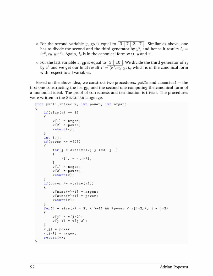
◦ For the second variable y, gp is equal to 3 7 2 7 . Similar as above, onehas to divide the second and the third generator by y6, and hence it results I2 =(x2, xy, yz10). Again, I2 is in the canonical form w.r.t. y and x.
◦ For the last variable z, gp is equal to 3 10 . We divide the third generator of I2by z9 and we get our final result I ′ = (x2, xy, yz)., which is in the canonical formwith respect to all variables.
Based on the above idea, we construct two procedures: putIn and canonical − thefirst one constructing the list gp, and the second one computing the canonical form ofa monomial ideal. The proof of correctness and termination is trivial. The procedureswere written in the SINGULAR language.
proc putIn(intvec v, int power , int nrgen)
{
if(size(v) == 1)
{
v[1] = nrgen;
v[2] = power;
return(v);
}
int i,j;
if(power <= v[2])
{
for(j = size(v)+2; j >=3; j--)
{
v[j] = v[j-2];
}
v[1] = nrgen;
v[2] = power;
return(v);
}
if(power >= v[size(v)])
{
v[size(v)+1] = nrgen;
v[size(v)+1] = power;
return(v);
}
for(j = size(v) + 2; (j>=4) && (power < v[j-2]); j = j-2)
{
v[j] = v[j-2];
v[j-1] = v[j-3];
}
v[j] = power;
v[j-1] = nrgen;
return(v);
}
92 Adrian Popescu
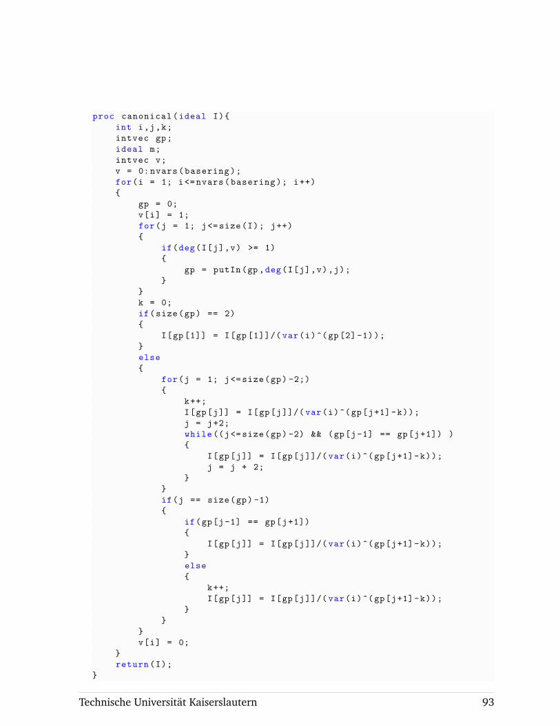
proc canonical(ideal I){
int i,j,k;
intvec gp;
ideal m;
intvec v;
v = 0:nvars(basering);
for(i = 1; i<= nvars(basering); i++)
{
gp = 0;
v[i] = 1;
for(j = 1; j<=size(I); j++)
{
if(deg(I[j],v) >= 1)
{
gp = putIn(gp ,deg(I[j],v),j);
}
}
k = 0;
if(size(gp) == 2)
{
I[gp[1]] = I[gp [1]]/( var(i)^(gp[2]-1));
}
else
{
for(j = 1; j<=size(gp) -2;)
{
k++;
I[gp[j]] = I[gp[j]]/( var(i)^(gp[j+1]-k));
j = j+2;
while ((j<=size(gp) -2) && (gp[j-1] == gp[j+1]) )
{
I[gp[j]] = I[gp[j]]/( var(i)^(gp[j+1]-k));
j = j + 2;
}
}
if(j == size(gp) -1)
{
if(gp[j-1] == gp[j+1])
{
I[gp[j]] = I[gp[j]]/( var(i)^(gp[j+1]-k));
}
else
{
k++;
I[gp[j]] = I[gp[j]]/( var(i)^(gp[j+1]-k));
}
}
}
v[i] = 0;
}
return(I);
}
Technische Universitat Kaiserslautern 93

PART C
CONSTRUCTIVE GENERAL NERON
DESINGULARIZATION
Technische Universitat Kaiserslautern 95

INTRODUCTION
PART C starts with a small introduction on Artin Approximation and the GeneralNeron Desingularization. We give an algorithmic proof of this desingularization in thecase of Noetherian local domains of dimension 1, u : A → A′ is a regular morphism,B is a finite type A−algebra and v : B → A′ an A−morphism. Thus we find a smoothA−algebra C such that v factors through C (see Theorem C:2.0.2), that is a GeneralNeron Desingularization of B, v. The idea is nicely presented in 3 steps in the introduc-tion of [PfPo2] and we recall it here below:
In step 1 we reduce the problem to the case when HB/A ∩ A 6= 0, HB/A being theideal defining the nonsmooth locus of B over A. Let 0 6= d ∈ HB/A ∩ A. This meansgeometrically that SpecBd → SpecAd is smooth. In the second step we construct asmooth A-algebra D, A ⊂ D ⊂ A′ and an A-morphism v′ : B → D/d3D such that v ≡ v′
modulo d3A′. If A′ is the completion A of A we can use D = A. The third step resolvesthe singularity. If B = A[Y ]/I, Y = (Y1, . . . , Yn) then we can find f = (f1, . . . , fr),r ≤ n a system of polynomials from I, and an r × r-minor M of the Jacobian matrix(∂fi∂Yj
)such that d ≡ MN modulo I for some N ∈
((f) : I
), where (f) denotes the
ideal generated by the system f . Then v′(MN) = ds for some s ∈ 1 + dD. Assume
that M = det
(∂fi∂Yj
)1≤i,j≤r
. Let H be the matrix obtained by adding to(∂f
∂Y
)the
boarder block (0|Idn−r) and let G′ be the adjoined matrix of H and G = NG′. Considerin D[Y, T ], T = (T1, . . . , Tn) the ideal J =
((f, s(Y − y′)− dG(y′)T ) : d2
), where y′ ∈ Dn
is lifting v′(Y ). Then C is a suitable localization of the B ⊗A D-algebra D[Y, T ]/(I, J)and v extends to C by v(T ) = t = (1/d2)H(y′)
(v(Y )− y′
).
Consider the following example. Let A = Q[x](x), A′ = C JxK, B =A[Y1, Y2]
(Y 21 + Y 2
2 )and
a ∈ C a transcendental element over Q, u ∈ C JxK \ C[x](x) and u = a + x6u. Let vbe given by v(Y1) = xu, v(Y2) = xiu, where i =
√−1. In step 1 we change B by
B1 = A[Y1, Y2, Y3]/I, I = (Y 21 + Y 2
2 , x − 2Y1Y3) and extend v by v(Y3) = 1/(2u). Wehave 4Y 2
1 Y23 ∈ HB/A which implies d = x2 ∈ HB/A ∩ A. We define D = A[a, a−1, i] and
v′(Y ) = y′ = (xa, xia, 1/(2a)). This is step two.To understand step 3 we simplify the example taking B = A[Y1, Y2]/(Y1Y2 − x2),
u = 1 + x6u and v given by v(Y1) = xu, v(Y2) = x/u. Then d = x ∈ HB/A,
D = A, y′1 = x = y′2. We obtain H =
(Y2 Y10 1
), G = G′ =
(1 −Y10 Y2
), N = 1 and
J =((Y1Y2 − x2, Y1 − x− xT1 + x2T2, Y2 − x− x2T2) : x2
). This leads to
J = (xT1T2 − x2T 22 + T1, Y1 − x− xT1 + x2T2, Y2 − x− x2T2)
Technische Universitat Kaiserslautern 97
and we obtain that C ∼=(
A[T1, T2]
(xT1T2 − x2T 22 + T1)
)1+xT2
∼=(A[T2]
)1+xT2
is a smooth A-
algebra.The implementation of our algorithm is done in several examples of Chapter 3.Now let (A,m) be a Noetherian local ring of dimension 1, A′ = A, B a finite type
A−algebra and c ∈ N. Suppose that A is Henselian and the completion map A → A isregular. If A is a discrete valuation ring, then Greenberg [Gr] showed that there existsa linear map ν : N → N such that for each A-morphism v : B → A/mν(c) there existsan A-morphism v′ : B → A such that v′ ≡ v modulo mc, that is A has the strong ArtinApproximation Property (see [PfPo1],[DP2]).
Our Corollary C:2.0.20 shows that if A is Cohen−Macaulay and the Jacobian locusof B is not too small, then there exists a linear map as in Greenberg’s case of the formc→ 2e+ c, where e depends on the polynomial system of equations defining B.
98 Adrian Popescu
CHAPTER C:1
ARTIN APPROXIMATION AND GENERAL NERON DESINGULARIZATION
This chapter is based on the common work of the author together with D. Popescu,[APDP2]. We first introduce a couple of definitions needed in the next sections.
DEFINITION C:1.0.1.A ring morphism u : A → A′ of Noetherian rings has regular fibers if for all prime
ideals P ∈ SpecA the ring A′/PA′ is a regular ring, i.e. its localizations are regular localrings.
It has geometrically regular fibers if for all prime ideals P ∈ SpecA and all finitefield extensions K of the fraction field of A/P the ring K ⊗A/P A′/PA′ is regular.
A flat morphism of Noetherian rings u is regular if its fibers are geometrically regu-lar.
DEFINITION C:1.0.2.A local ring (A,m) is Henselian if the Implicit Function Theorem (C:1.0.3) holds in
A.A Henselian Noetherian local ring A is excellent if the completion map A → A is
regular.
THEOREM C:1.0.3(Implicit Function Theorem
).
Let F ∈ A Jx1, . . . , xn, yK such that F (x1, . . . , xn, 0) ∈ 〈x1, . . . , xn〉 and∂F
∂y(x1, . . . , xn, 0) 6∈ 〈x1, . . . , xn〉. Then there exists a unique
y(x1, . . . , xn) ∈ 〈x1, . . . , xn〉A Jx1, . . . , xnK
such thatF(x1, . . . , xn, y(x1, . . . , xn)
)= 0.
DEFINITION C:1.0.4.A Noetherian local ring (A,m) has the Artin approximation property if every finite
system of polynomial equations over A has a solution in A if and only if has a solutionin the completion A of A.
In fact A has the Artin approximation property if and only if every finite system f ofpolynomial equations overA in Y = (Y1, . . . , Yn) has its solutions inA dense with respectto the m-adic topology in the set of its solutions in A; that is, for every solution y of f inA and every positive integer c there exists a solution y in A such that y ≡ y modulo mcA.
Technische Universitat Kaiserslautern 99
DEFINITION C:1.0.5.Let K be a field. We denote by K 〈x〉, where x = x1, . . . , xn, the algebraic power
series ring over K, i.e. the algebraic closure of the polynomial ring K[x] in the formalpower series ring K JxK.
M. Artin showed in [Artin1] that the algebraic power series over a field has theproperty of Artin approximation. He also set in [Artin2] several conjectures, one ofthem is solved in the following theorem.
THEOREM C:1.0.6([DP2, Theorem 1.3]
).
An excellent Henselian local ring has the property of Artin approximation property.
The proof is based on the existence of the so-called General Neron Desingularization,that is the following theorem generalizes the Neron Desingularization [Ne], [Artin1].
THEOREM C:1.0.7(General Neron Desingularization, Popescu [DP1], [DP2], [DP3],
Swan [Sw]).
Let u : A → A′ be a regular morphism of Noetherian rings and B a finite type A-algebra. Then any A-morphism v : B → A′ factors through a smooth A-algebra C, that isv is a composite A-morphism B → C → A′.
REMARK C:1.0.8. Using this theorem we get an easy proof of Theorem C:1.0.6. Indeed,let f be a finite system of polynomial equations over A in Y = (Y1, . . . , Yn) and y asolution of f in A. Set B = A[Y ]/(f) and let the morphism
v : B // A
Y � // y.
By Theorem C:1.0.7, v factors through a smooth A-algebra C, that is v is a com-posite A-morphism B → C → A′. Thus changing B by C we may reduce the problemto the case when B is smooth over A. Then 1 ∈
((g) : I
)M for some polynomials
g = (g1, . . . , gr) from (f) and a r × r-minor M of the Jacobian matrix(∂g
∂Y
). Thus
g(y) = 0 and M(y) is invertible. By the Implicit Function Theorem there exists y ∈ Asuch that y ≡ y modulo mA.
The main purpose of this part is to give an algorithmic proof of Theorem C:1.0.7when A,A′ are one dimensional Noetherian local domains and A ⊃ Q. This is publishedin [APDP2]. An extension of our algorithm can be found in [PfPo2]. We may take thesame General Neron Desingularization for v, v′ : B → A′ if they are closed enough asExamples C:2.0.3 and C:2.0.9 show. This remark was basic in [DP8, Theorem 10]. Thelast section of this chapter computes the General Neron Desingularization in severalexamples. We should point that the General Neron Desingularization is not unique andit is better to speak above about a General Neron Desingularization.
100 Adrian Popescu
DEFINITION C:1.0.9.A Noetherian local ring (A,m) has the strong Artin approximation property if for
every finite system of polynomial equations f in Y = (Y1, . . . , Yn) over A there exists amap ν : N→ N with the following property
If y′ ∈ An satisfies f(y′) ≡ 0 modulo mν(c), c ∈ N, then there exists a solutiony ∈ An of f with y ≡ y′ modulo mc.
M. Greenberg [Gr] proved that excellent Henselian discrete valuation rings havethe strong Artin approximation property and ν is linear in this case. M. Artin [Artin1]showed that the algebraic power series ring over a field has also the strong Artin ap-proximation property. In [PfPo1] (see also [KMPPR]) it states that Noetherian completelocal rings have the strong Artin approximation property and it follows that A has thestrong Artin approximation property if it has the Artin approximation property. ThusTheorem C:1.0.6 gives that excellent Henselian local rings have the strong Artin ap-proximation property. An easy proof of this fact is given in [DP2, 4.5] using TheoremC:1.0.7 and ultrapower methods.
When A′ is the completion of a Cohen-Macaulay local ring A of dimension 1 weshow that we may have a linear Artin function as it happens in the Greenberg’s case(see C:2.0.19). More precisely, the Artin function is given by c 7→ 2e + c, where edepends from the polynomial system of equations defining B. Later this result wasextended in [PfPo2] in the case of non Cohen-Macaulay local rings of one dimension. IfdimA > 1 then ν may be not linear as shows [Ro].
Technische Universitat Kaiserslautern 101

CHAPTER C:2
A METHOD TO COMPUTE A GENERAL NERON DESINGULARIZATION IN THE
FRAME OF ONE DIMENSIONAL LOCAL DOMAINS
Let u : A → A′ be a flat morphism of Noetherian local domains of dimension 1.Suppose that A ⊃ Q and the maximal ideal m of A generates the maximal ideal of A′.Then u is regular morphism. Moreover, we suppose that there exist canonical inclusionsk = A/m→ A, k′ = A′/mA′ → A′ such that u(k) ⊂ k′.
Let B = A[Y ]/I, Y = (Y1, . . . , Yn). If f = (f1, . . . , fr), r ≤ n is a system of polynomialsfrom I then we can define the ideal ∆f generated by all r × r−minors of the Jacobian
matrix(∂fi∂Yj
). After Elkik [El], let HB/A be the radical of the ideal
∑f
((f) : I
)∆fB,
where the sum is taken over all systems of polynomials f from I with r ≤ n. ThenBP , P ∈ SpecB is essentially smooth over A if and only if P 6⊃ HB/A by the Jacobiancriterion for smoothness. Thus HB/A measures the non smooth locus of B over A.
DEFINITION C:2.0.1.B is standard smooth over A if there exists f in I as above such that
1 ∈((f) : I
)∆fB.
The aim of this chapter is to give an easy algorithmic proof of the following theorem.
THEOREM C:2.0.2.Any A-morphism v : B → A′ factors through a standard smooth A-algebra B′.
If A is essentially of finite type over Q, then the ideal HB/A can be computed inSINGULAR by following its definition but it is easier to describe only the ideal∑
f
((f) : I
)∆fB defined above. This is the case considered in our algorithmic part,
let us say A ∼= k[x]/F for some variables x = (x1, . . . xt), and the completion of A′ is KJxK/Ffor some field extension k ⊂ K. When v is defined by polynomials y from K[x] thenour problem is easy. Let L be the field obtained by adjoining to k all coefficients of y.Then R = L[x]/F is a subring of A′ containing Im v which is essentially smooth over A.Then we may take B′ as a standard smooth A-algebra such that R is a localization ofB′. Consequently we suppose usually that y is not polynomial defined and moreover Lis not a finite type field extension of k.
We may suppose that v(HB/A) 6= 0. Indeed, if v(HB/A) = 0 then v induces an A-morphism v′ : B′ = B/HB/A → A′ and we may change (B, v) by (B′, v′). Applying this
Technische Universitat Kaiserslautern 103
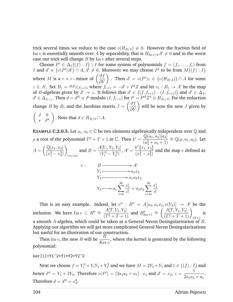
trick several times we reduce to the case v(HB/A) 6= 0. However the fraction field ofIm v is essentially smooth over A by separability, that is HIm v/AA
′ 6= 0 and in the worstcase our trick will change B by Im v after several steps.
Choose P ′ ∈ ∆f
((f) : I
)\ I for some system of polynomials f = (f1, . . . , fr) from
I and d′ ∈(v(P ′)A′
)∩ A, d′ 6= 0. Moreover we may choose P ′ to be from M
((f) : I
)where M is a r × r−minor of
(∂f
∂Y
). Then d′ = v(P ′)z ∈
(v(HB/A)
)∩ A for some
z ∈ A′. Set B1 = B[Z]/(fr+1), where fr+1 = −d′ + P ′Z and let v1 : B1 → A′ be the mapof B-algebras given by Z → z. It follows that d′ ∈
((f, fr+1) : (I, fr+1)
)and d′ ∈ ∆f ,
d′ ∈ ∆fr+1. Then d = d′2 ≡ P modulo (I, fr+1) for P = P ′2Z2 ∈ HB1/A. For the reduction
change B by B1 and the Jacobian matrix J =
(∂f
∂Y
)will be now the new J given by(
J 0∗ P ′
). Note that d ∈ HB/A ∩ A.
EXAMPLE C:2.0.3. Let a1, a2 ∈ C be two elements algebraically independent over Q and
ρ a root of the polynomial T 2 + T + 1 in C. Then k′ =Q(a1, a2)[a3]
(a23 + a3 + 1)∼= Q(ρ, a1, a2). Let
A =
(Q[x1, x2]
(x31 − x22)
)(x1,x2)
and B =A[Y1, Y2, Y3]
(Y 31 − Y 3
2 ), A′ =
k′ Jx1, x2K(x31 − x22)
and the map v defined as
v : B // A′
Y1� // a1x2
Y2� // a1a3x2
Y3� // a1
30∑i=0
xi1i!
+ a2x2
50∑i=31
xi1i!
This is an easy example. Indeed, let v′′ : B′′ = A[a3, a1x2, v(Y3)
]→ A′ be the
inclusion. We have Im v ⊂ B′′ ∼=A[T, Y1, Y3]
(T 2 + T + 1)and B′′2a3+1
∼=(A[T, Y1, Y3]
(T 2 + T + 1)
)2T+1
is
a smooth A-algebra, which could be taken as a General Neron Desingularization of B.Applying our algorithm we will get more complicated General Neron Desingularizationsbut useful for an illustration of our construction.
Then Im v, the new B will beB
Ker v, where the kernel is generated by the following
polynomial:
ker[1]=Y1^2+Y1*Y2+Y2^2
Next we choose f = Y 21 +Y1Y2 +Y 2
2 and we have M = 2Y2 +Y1 and 1 ∈((f) : I
)and
hence P ′ = Y1 + 2Y2. Therefore v(P ′) = (2a1a3 + a1) · x2 and d′ = x2, z =1
2a1a3 + a1.
Therefore d = d′2 = x22.
104 Adrian Popescu
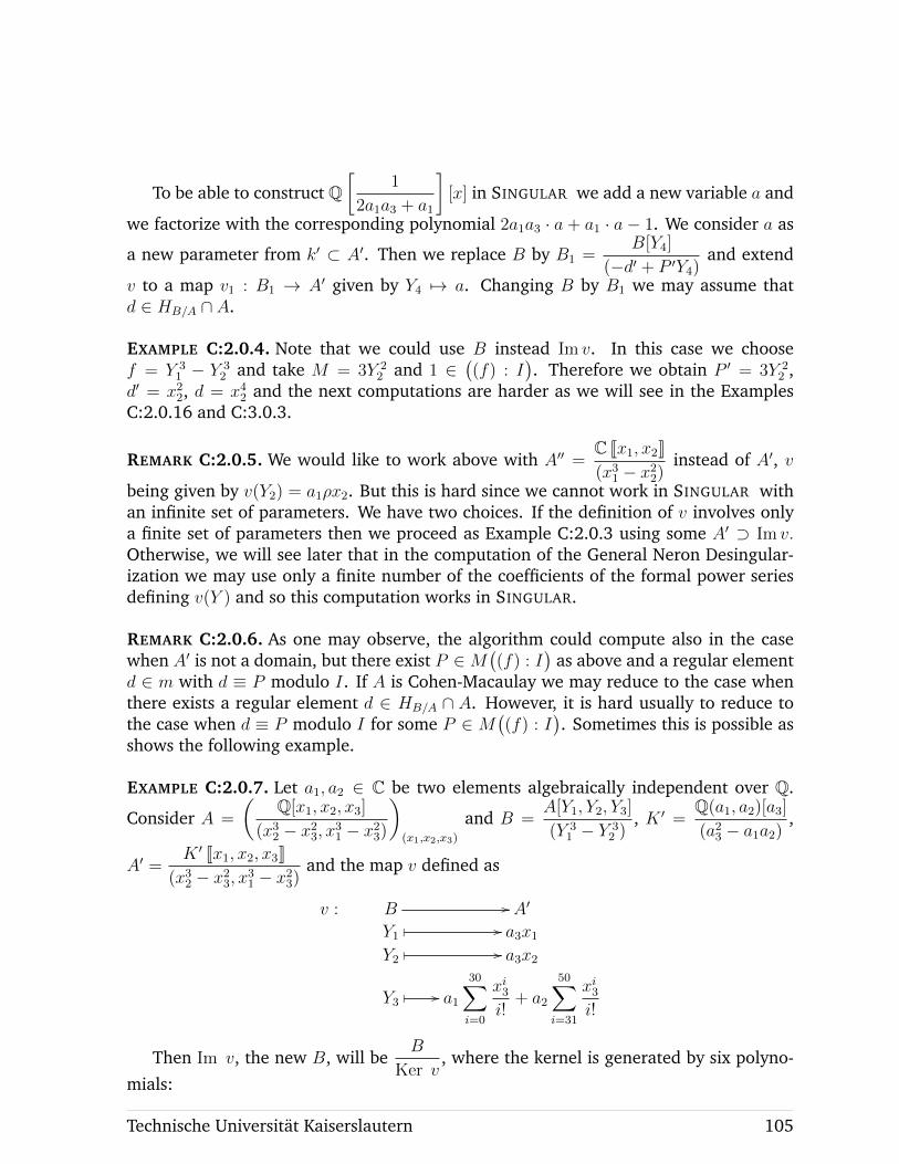
To be able to construct Q[
1
2a1a3 + a1
][x] in SINGULAR we add a new variable a and
we factorize with the corresponding polynomial 2a1a3 · a + a1 · a− 1. We consider a as
a new parameter from k′ ⊂ A′. Then we replace B by B1 =B[Y4]
(−d′ + P ′Y4)and extend
v to a map v1 : B1 → A′ given by Y4 7→ a. Changing B by B1 we may assume thatd ∈ HB/A ∩ A.
EXAMPLE C:2.0.4. Note that we could use B instead Im v. In this case we choosef = Y 3
1 − Y 32 and take M = 3Y 2
2 and 1 ∈((f) : I
). Therefore we obtain P ′ = 3Y 2
2 ,d′ = x22, d = x42 and the next computations are harder as we will see in the ExamplesC:2.0.16 and C:3.0.3.
REMARK C:2.0.5. We would like to work above with A′′ =C Jx1, x2K(x31 − x22)
instead of A′, v
being given by v(Y2) = a1ρx2. But this is hard since we cannot work in SINGULAR withan infinite set of parameters. We have two choices. If the definition of v involves onlya finite set of parameters then we proceed as Example C:2.0.3 using some A′ ⊃ Im v.Otherwise, we will see later that in the computation of the General Neron Desingular-ization we may use only a finite number of the coefficients of the formal power seriesdefining v(Y ) and so this computation works in SINGULAR.
REMARK C:2.0.6. As one may observe, the algorithm could compute also in the casewhen A′ is not a domain, but there exist P ∈M
((f) : I
)as above and a regular element
d ∈ m with d ≡ P modulo I. If A is Cohen-Macaulay we may reduce to the case whenthere exists a regular element d ∈ HB/A ∩ A. However, it is hard usually to reduce tothe case when d ≡ P modulo I for some P ∈ M
((f) : I
). Sometimes this is possible as
shows the following example.
EXAMPLE C:2.0.7. Let a1, a2 ∈ C be two elements algebraically independent over Q.
Consider A =
(Q[x1, x2, x3]
(x32 − x23, x31 − x23)
)(x1,x2,x3)
and B =A[Y1, Y2, Y3]
(Y 31 − Y 3
2 ), K ′ =
Q(a1, a2)[a3]
(a23 − a1a2),
A′ =K ′ Jx1, x2, x3K
(x32 − x23, x31 − x23)and the map v defined as
v : B // A′
Y1� // a3x1
Y2� // a3x2
Y3� // a1
30∑i=0
xi3i!
+ a2
50∑i=31
xi3i!
Then Im v, the new B, will beB
Ker v, where the kernel is generated by six polyno-
mials:
Technische Universitat Kaiserslautern 105
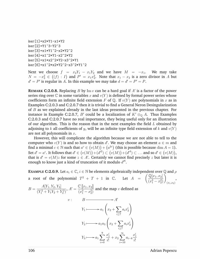
ker[1]=x2*Y1-x1*Y2
ker[2]=Y1^3-Y2^3
ker[3]=x1*Y1^2-x2*Y2^2
ker[4]=x1^2*Y1-x2^2*Y2
ker[5]=x1*x2^2*Y2-x3^2*Y1
ker[6]=x1^2*x2*Y2^2-x3^2*Y1^2
Next we choose f = x2Y1 − x1Y2 and we have M = −x1. We may takeN = −x23 ∈
((f) : I
)and P ′ = x1x
23. Note that x1 − x2 is a zero divisor in A but
d′ = P ′ is regular in A. In this example we may take d = d′ = P ′ = P .
REMARK C:2.0.8. Replacing B by Im v can be a hard goal if A′ is a factor of the powerseries ring over C in some variables x and v(Y ) is defined by formal power series whosecoefficients form an infinite field extension F of Q. If v(Y ) are polynomials in x as inExamples C:2.0.3 and C:2.0.7 then it is trivial to find a General Neron Desingularizationof B as we explained already in the last ideas presented in the previous chapter. Forinstance in Example C:2.0.7, B′ could be a localization of K ′ ⊗Q A. Thus ExamplesC:2.0.3 and C:2.0.7 have no real importance, they being useful only for an illustrationof our algorithm. This is the reason that in the next examples the field L obtained byadjoining to k all coefficients of y, will be an infinite type field extension of k and v(Y )are not all polynomials in x.
However, this will complicate the algorithm because we are not able to tell to thecomputer who v(Y ) is and so how to obtain d′. We may choose an element a ∈ m andfind a minimal c ∈ N such that ac ∈
(v(M)
)+(a2c)
(this is possible because dimA = 1).Set d′ = ac. It follows that d′ ∈
(v(M)
)+(d′2) ⊂
(v(M)
)+(d′4) ⊂ . . . and so d′ ∈
(v(M)
),
that is d′ = v(M)z for some z ∈ A′. Certainly we cannot find precisely z but later it isenough to know just a kind of truncation of it modulo d′6.
EXAMPLE C:2.0.9. Let ai ∈ C, i ∈ N be elements algebraically independent over Q and ρ
a root of the polynomial T 2 + T + 1 in C. Let A =
(Q[x1, x2]
(x31 − x22)
)(x1,x2)
,
B =A[Y1, Y2, Y3]
(Y 21 + Y1Y2 + Y 2
2 ), A′ =
C Jx1, x2K(x31 − x22)
and the map v defined as
v : B // A′
Y1� // a1
(x2 +
∑i≥7
aixi2
)
Y2� // a1a3
(x2 +
∑i≥7
aixi2
)
Y3� // a1
9∑i=0
xi1i!
+ x2
∞∑i=10
ai−8xi1i!
106 Adrian Popescu
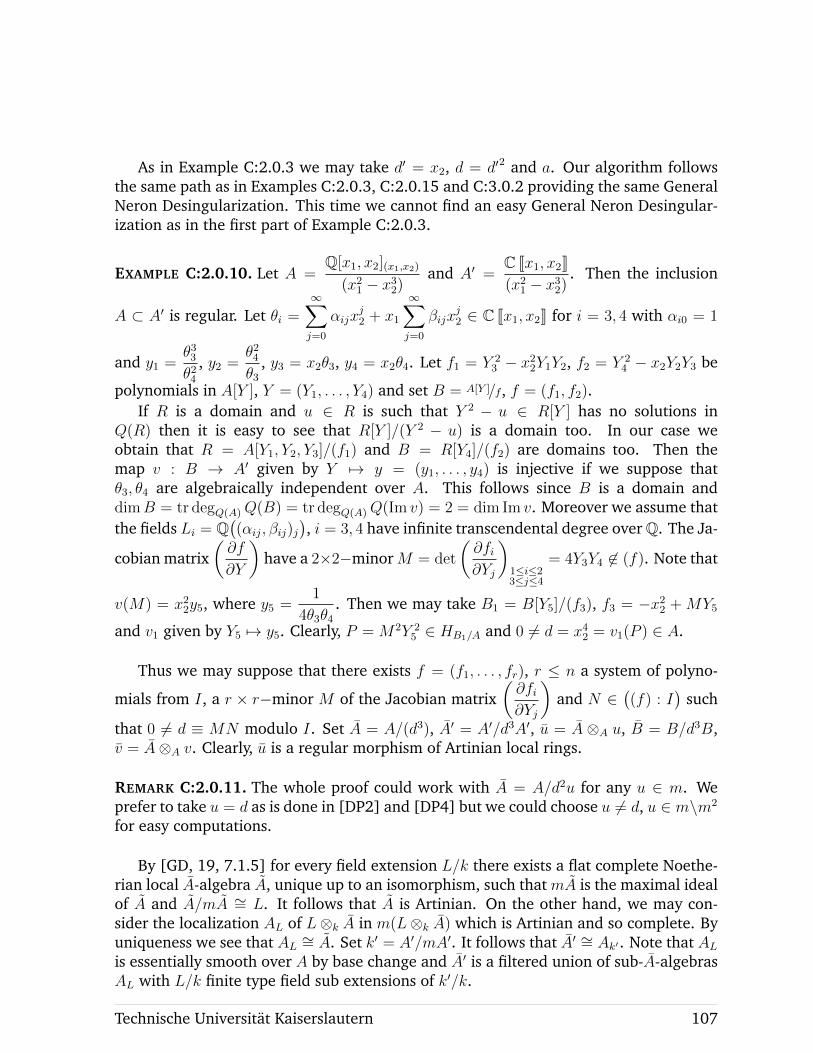
As in Example C:2.0.3 we may take d′ = x2, d = d′2 and a. Our algorithm followsthe same path as in Examples C:2.0.3, C:2.0.15 and C:3.0.2 providing the same GeneralNeron Desingularization. This time we cannot find an easy General Neron Desingular-ization as in the first part of Example C:2.0.3.
EXAMPLE C:2.0.10. Let A =Q[x1, x2](x1,x2)
(x21 − x32)and A′ =
C Jx1, x2K(x21 − x32)
. Then the inclusion
A ⊂ A′ is regular. Let θi =∞∑j=0
αijxj2 + x1
∞∑j=0
βijxj2 ∈ C Jx1, x2K for i = 3, 4 with αi0 = 1
and y1 =θ33θ24
, y2 =θ24θ3
, y3 = x2θ3, y4 = x2θ4. Let f1 = Y 23 − x22Y1Y2, f2 = Y 2
4 − x2Y2Y3 be
polynomials in A[Y ], Y = (Y1, . . . , Y4) and set B = A[Y ]/f, f = (f1, f2).If R is a domain and u ∈ R is such that Y 2 − u ∈ R[Y ] has no solutions in
Q(R) then it is easy to see that R[Y ]/(Y 2 − u) is a domain too. In our case weobtain that R = A[Y1, Y2, Y3]/(f1) and B = R[Y4]/(f2) are domains too. Then themap v : B → A′ given by Y 7→ y = (y1, . . . , y4) is injective if we suppose thatθ3, θ4 are algebraically independent over A. This follows since B is a domain anddimB = tr degQ(A)Q(B) = tr degQ(A)Q(Im v) = 2 = dim Im v. Moreover we assume thatthe fields Li = Q
((αij, βij)j
), i = 3, 4 have infinite transcendental degree over Q. The Ja-
cobian matrix(∂f
∂Y
)have a 2×2−minorM = det
(∂fi∂Yj
)1≤i≤23≤j≤4
= 4Y3Y4 6∈ (f). Note that
v(M) = x22y5, where y5 =1
4θ3θ4. Then we may take B1 = B[Y5]/(f3), f3 = −x22 + MY5
and v1 given by Y5 7→ y5. Clearly, P = M2Y 25 ∈ HB1/A and 0 6= d = x42 = v1(P ) ∈ A.
Thus we may suppose that there exists f = (f1, . . . , fr), r ≤ n a system of polyno-
mials from I, a r × r−minor M of the Jacobian matrix(∂fi∂Yj
)and N ∈
((f) : I
)such
that 0 6= d ≡ MN modulo I. Set A = A/(d3), A′ = A′/d3A′, u = A ⊗A u, B = B/d3B,v = A⊗A v. Clearly, u is a regular morphism of Artinian local rings.
REMARK C:2.0.11. The whole proof could work with A = A/d2u for any u ∈ m. Weprefer to take u = d as is done in [DP2] and [DP4] but we could choose u 6= d, u ∈ m\m2
for easy computations.
By [GD, 19, 7.1.5] for every field extension L/k there exists a flat complete Noethe-rian local A-algebra A, unique up to an isomorphism, such that mA is the maximal idealof A and A/mA ∼= L. It follows that A is Artinian. On the other hand, we may con-sider the localization AL of L⊗k A in m(L⊗k A) which is Artinian and so complete. Byuniqueness we see that AL ∼= A. Set k′ = A′/mA′. It follows that A′ ∼= Ak′. Note that ALis essentially smooth over A by base change and A′ is a filtered union of sub-A-algebrasAL with L/k finite type field sub extensions of k′/k.
Technische Universitat Kaiserslautern 107
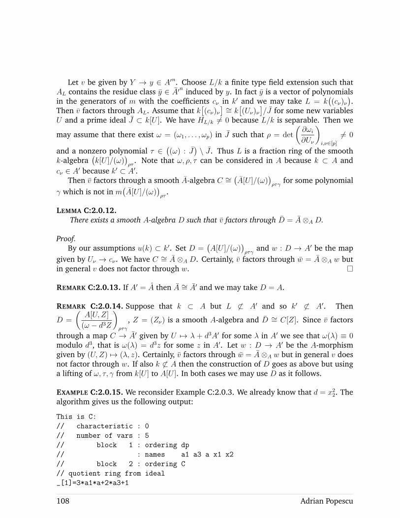
Let v be given by Y → y ∈ A′n. Choose L/k a finite type field extension such thatAL contains the residue class y ∈ A′n induced by y. In fact y is a vector of polynomialsin the generators of m with the coefficients cν in k′ and we may take L = k
((cν)ν
).
Then v factors through AL. Assume that k[(cν)ν
] ∼= k[(Uν)ν
]/J for some new variables
U and a prime ideal J ⊂ k[U ]. We have HL/k 6= 0 because L/k is separable. Then we
may assume that there exist ω = (ω1, . . . , ωp) in J such that ρ = det
(∂ωi∂Uν
)i,ν∈[p]
6= 0
and a nonzero polynomial τ ∈((ω) : J
)\ J . Thus L is a fraction ring of the smooth
k-algebra(k[U ]/(ω)
)ρτ
. Note that ω, ρ, τ can be considered in A because k ⊂ A andcν ∈ A′ because k′ ⊂ A′.
Then v factors through a smooth A-algebra C ∼=(A[U ]/(ω)
)ρτγ
for some polynomialγ which is not in m
(A[U ]/(ω)
)ρτ
.
LEMMA C:2.0.12.There exists a smooth A-algebra D such that v factors through D = A⊗A D.
Proof.By our assumptions u(k) ⊂ k′. Set D =
(A[U ]/(ω)
)ρτγ
and w : D → A′ be the mapgiven by Uν → cν . We have C ∼= A ⊗A D. Certainly, v factors through w = A ⊗A w butin general v does not factor through w.
REMARK C:2.0.13. If A′ = A then A ∼= A′ and we may take D = A.
REMARK C:2.0.14. Suppose that k ⊂ A but L 6⊂ A′ and so k′ 6⊂ A′. Then
D =
(A[U,Z]
(ω − d3Z
)ρτγ
, Z = (Zν) is a smooth A-algebra and D ∼= C[Z]. Since v factors
through a map C → A′ given by U 7→ λ + d3A′ for some λ in A′ we see that ω(λ) ≡ 0modulo d3, that is ω(λ) = d3z for some z in A′. Let w : D → A′ be the A-morphismgiven by (U,Z) 7→ (λ, z). Certainly, v factors through w = A⊗A w but in general v doesnot factor through w. If also k 6⊂ A then the construction of D goes as above but usinga lifting of ω, τ, γ from k[U ] to A[U ]. In both cases we may use D as it follows.
EXAMPLE C:2.0.15. We reconsider Example C:2.0.3. We already know that d = x22. Thealgorithm gives us the following output:
This is C:
// characteristic : 0
// number of vars : 5
// block 1 : ordering dp
// : names a1 a3 a x1 x2
// block 2 : ordering C
// quotient ring from ideal
_[1]=3*a1*a+2*a3+1
108 Adrian Popescu
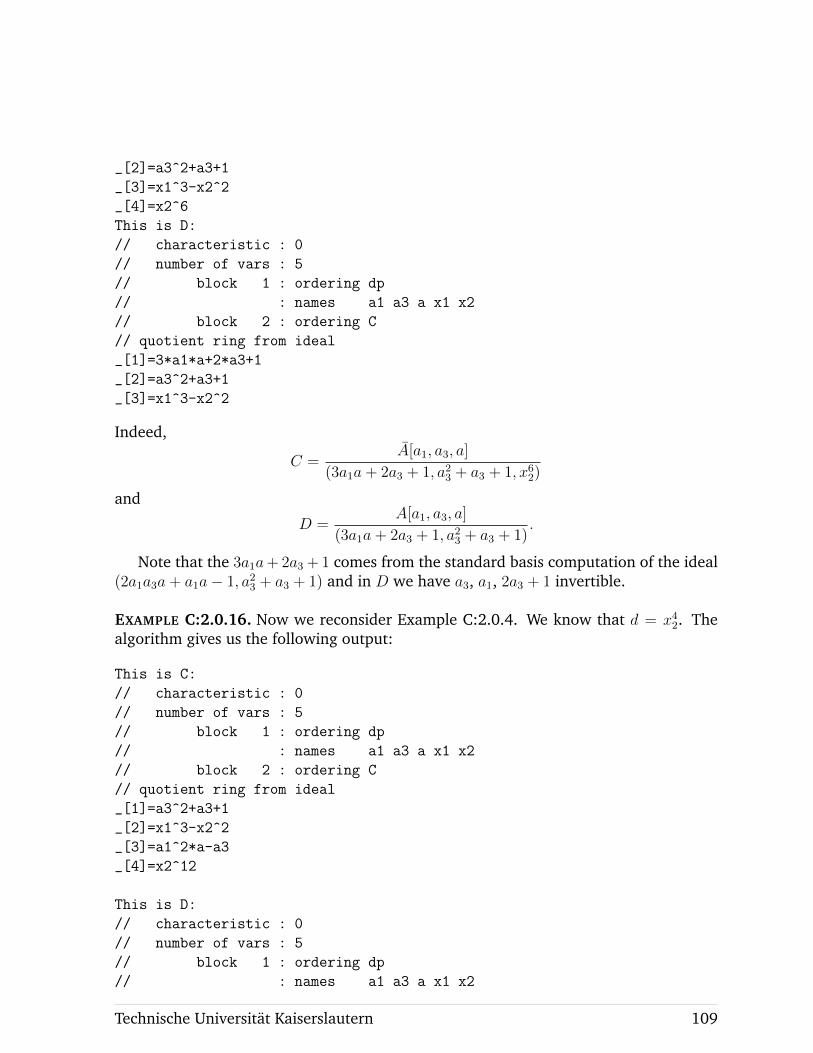
_[2]=a3^2+a3+1
_[3]=x1^3-x2^2
_[4]=x2^6
This is D:
// characteristic : 0
// number of vars : 5
// block 1 : ordering dp
// : names a1 a3 a x1 x2
// block 2 : ordering C
// quotient ring from ideal
_[1]=3*a1*a+2*a3+1
_[2]=a3^2+a3+1
_[3]=x1^3-x2^2
Indeed,
C =A[a1, a3, a]
(3a1a+ 2a3 + 1, a23 + a3 + 1, x62)
and
D =A[a1, a3, a]
(3a1a+ 2a3 + 1, a23 + a3 + 1).
Note that the 3a1a+ 2a3 + 1 comes from the standard basis computation of the ideal(2a1a3a+ a1a− 1, a23 + a3 + 1) and in D we have a3, a1, 2a3 + 1 invertible.
EXAMPLE C:2.0.16. Now we reconsider Example C:2.0.4. We know that d = x42. Thealgorithm gives us the following output:
This is C:
// characteristic : 0
// number of vars : 5
// block 1 : ordering dp
// : names a1 a3 a x1 x2
// block 2 : ordering C
// quotient ring from ideal
_[1]=a3^2+a3+1
_[2]=x1^3-x2^2
_[3]=a1^2*a-a3
_[4]=x2^12
This is D:
// characteristic : 0
// number of vars : 5
// block 1 : ordering dp
// : names a1 a3 a x1 x2
Technische Universitat Kaiserslautern 109
// block 2 : ordering C
// quotient ring from ideal
_[1]=a3^2+a3+1
_[2]=x1^3-x2^2
_[3]=a1^2*a-a3
Indeed,
C =A[a1, a3, a]
(a23 + a3 + 1, a21a− a3, x122 )
and
D =A[a1, a3, a]
(a23 + a3 + 1, a21a− a3).
Note that a3, a1 are invertible in D.
EXAMPLE C:2.0.17. In the case of Example C:2.0.7 we obtain the following output:
This is C:
// characteristic : 0
// number of vars : 5
// block 1 : ordering dp
// : names a1 a3 x1 x2 x3
// block 2 : ordering C
// quotient ring from ideal
_[1]=x2^3-x3^2
_[2]=x1^3-x3^2
_[3]=x3^8
This is D:
// characteristic : 0
// number of vars : 5
// block 1 : ordering dp
// : names a1 a3 x1 x2 x3
// block 2 : ordering C
// quotient ring from ideal
_[1]=x2^3-x3^2
_[2]=x1^3-x3^2
Indeed this is the case since we have d = x1x23 and hence
C =A[a1, a3]
(x83)
andD = A[a1, a3].
110 Adrian Popescu
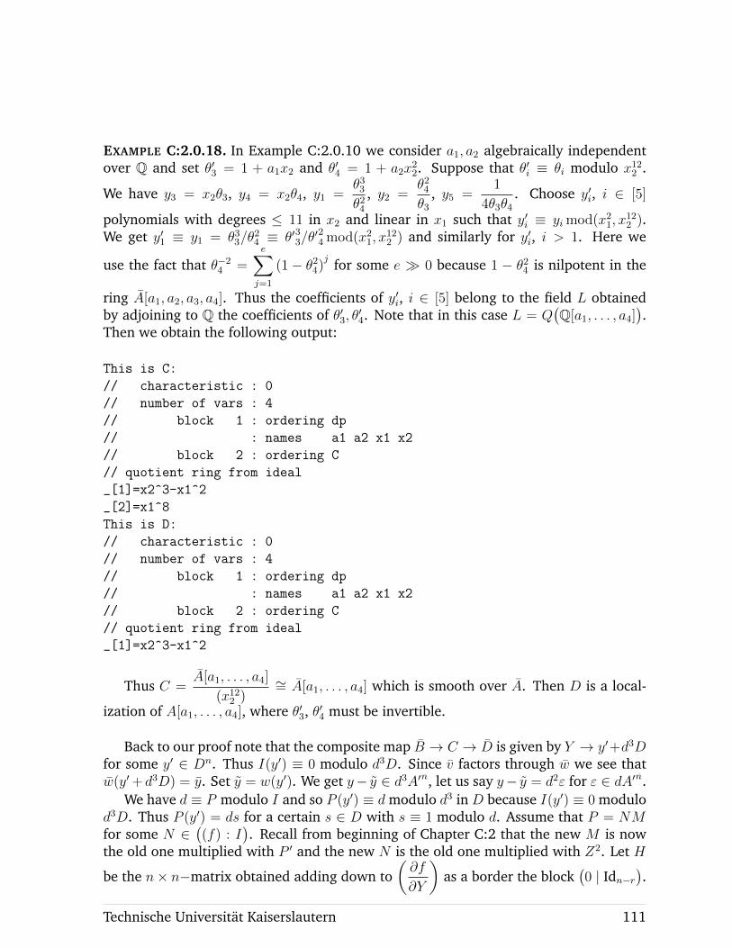
EXAMPLE C:2.0.18. In Example C:2.0.10 we consider a1, a2 algebraically independentover Q and set θ′3 = 1 + a1x2 and θ′4 = 1 + a2x
22. Suppose that θ′i ≡ θi modulo x122 .
We have y3 = x2θ3, y4 = x2θ4, y1 =θ33θ24
, y2 =θ24θ3
, y5 =1
4θ3θ4. Choose y′i, i ∈ [5]
polynomials with degrees ≤ 11 in x2 and linear in x1 such that y′i ≡ yi mod(x21, x122 ).
We get y′1 ≡ y1 = θ33/θ24 ≡ θ′33/θ
′24 mod(x21, x
122 ) and similarly for y′i, i > 1. Here we
use the fact that θ−24 =e∑j=1
(1− θ24)j for some e � 0 because 1 − θ24 is nilpotent in the
ring A[a1, a2, a3, a4]. Thus the coefficients of y′i, i ∈ [5] belong to the field L obtainedby adjoining to Q the coefficients of θ′3, θ
′4. Note that in this case L = Q
(Q[a1, . . . , a4]
).
Then we obtain the following output:
This is C:
// characteristic : 0
// number of vars : 4
// block 1 : ordering dp
// : names a1 a2 x1 x2
// block 2 : ordering C
// quotient ring from ideal
_[1]=x2^3-x1^2
_[2]=x1^8
This is D:
// characteristic : 0
// number of vars : 4
// block 1 : ordering dp
// : names a1 a2 x1 x2
// block 2 : ordering C
// quotient ring from ideal
_[1]=x2^3-x1^2
Thus C =A[a1, . . . , a4]
(x122 )∼= A[a1, . . . , a4] which is smooth over A. Then D is a local-
ization of A[a1, . . . , a4], where θ′3, θ′4 must be invertible.
Back to our proof note that the composite map B → C → D is given by Y → y′+d3Dfor some y′ ∈ Dn. Thus I(y′) ≡ 0 modulo d3D. Since v factors through w we see thatw(y′+ d3D) = y. Set y = w(y′). We get y− y ∈ d3A′n, let us say y− y = d2ε for ε ∈ dA′n.
We have d ≡ P modulo I and so P (y′) ≡ d modulo d3 in D because I(y′) ≡ 0 modulod3D. Thus P (y′) = ds for a certain s ∈ D with s ≡ 1 modulo d. Assume that P = NMfor some N ∈
((f) : I
). Recall from beginning of Chapter C:2 that the new M is now
the old one multiplied with P ′ and the new N is the old one multiplied with Z2. Let H
be the n× n−matrix obtained adding down to(∂f
∂Y
)as a border the block
(0 | Idn−r
).
Technische Universitat Kaiserslautern 111
Let G′ be the adjoint matrix of H and G = NG′. We have
GH = HG = NM Idn = P Idn
and sodsIdn = P (y′)Idn = G(y′)H(y′).
Then t := H(y′)ε ∈ dA′n satisfies
G(y′)t = P (y′)ε = dsε
and sos(y − y) = dw
(G(y′)
)t.
Leth = s(Y − y′)− dG(y′)T, (C:2.1)
where T = (T1, . . . , Tn) are new variables. The kernel of the map ϕ : D[Y, T ]→ A′ givenby Y → y, T → t contains h. Since
s(Y − y′) ≡ dG(y′)T modulo h
andf(Y )− f(y′) ≡
∑j
∂f
∂Yj(y′)(Yj − y′j)
modulo higher order terms in Yj − y′j by Taylor’s formula we see that for p = maxi deg fiwe have
spf(Y )− spf(y′) ≡∑j
sp−1d∂f
∂Yj(y′)Gj(y
′)Tj + d2Q = sp−1dP (y′)T + d2Q (C:2.2)
modulo h where Q ∈ T 2D[T ]r. This is because (∂f/∂Y )G = (P Idr|0). We have f(y′) =d2b for some b ∈ dDr. Then
gi = spbi + spTi +Qi, i ∈ [r] (C:2.3)
is in the kernel of ϕ because d2ϕ(g) = d2g(t) ∈(h(y, t), f(y)
)= (0).
Set E =D[Y, T ]
(I, g, h)and let ψ : E → A′ be the map induced by ϕ. Clearly, v factors
through ψ because v is the composed map B → B ⊗A D ∼= D[Y ]/I → Eψ−→ A′.
Note that the r × r−minor s′ of (∂g/∂T ) given by the first r−variables T is fromsrp + (T ) ⊂ 1 + (d, T )D[Y, T ] because Q ∈ (T )2. Then U =
(D[Y, T ]/(h, g)
)ss′
is smoothover D. We claim that I ⊂ (h, g)D[Y, T ]ss′s′′ for some other s′′ ∈ 1 + (d, T )D[Y, T ].Indeed, we have PI ⊂ (h, g)D[Y, T ]s and so P
(y′ + s−1dG(y′)T
)I ⊂ (h, g)D[Y, T ]s.
Since P(y′ + s−1dG(y′)T
)∈ P (y′) + d(T ) we get P
(y′ + s−1dG(y′)T
)= ds′′ for some
s′′ ∈ 1+(d, T )D[Y, T ]. It follows that s′′I ⊂ (h, g)D[Y, T ]ss′ because d is regular in U , the
112 Adrian Popescu
map D → U being flat, and so I ⊂ (h, g)D[Y, T ]ss′s′′. Thus Ess′s′′ ∼= Us′′ is a B-algebrawhich is also standard smooth over D and A.
As w(s) ≡ 1 modulo d and w(s′), w(s′′) ≡ 1 modulo (d, t), d, t ∈ mA′ we see thatw(s), w(s′), w(s′′) are invertible because A′ is local and ψ (thus v) factors through thestandard smooth A-algebra Ess′s′′.
Let (A,m) be a Cohen-Macaulay local ring (for example a reduced ring) of dimension1, A′ = A the completion of A, B = A[Y ]/I, Y = (Y1, . . . , Yn) a finite type A−algebraand c, e ∈ N. Suppose that there exist f = (f1, . . . , fr) in I, a r × r−minor M of the
Jacobian matrix(∂f
∂Y
), N ∈
((f) : I
)and an A-morphism v : B → A/m2e+c such that(
v(MN))⊃ me/m2e+c.
THEOREM C:2.0.19.Then there exists an A-morphism v′ : B → A such that v′ ≡ v modulo mc, that is
v′(Y + I) ≡ v(Y + I) modulo mc.
Proof.We note that the proof of Theorem C:2.0.2 can work somehow in this case. Let
y′ ∈ An be an element inducing v(Y + I). Then
me ⊂((MN)(y′)
)+m2e+c ⊂
((MN)(y′)
)+m3e+2c ⊂ . . .
by hypothesis. It follows that me ⊂((MN)(y′)
). Since A is Cohen-Macaulay we see
that me contains a regular element of A and so (MN)(y′) must be regular too.Set d = (MN)(y′). Next we follow the proof of Theorem C:2.0.2 with D = A, s = 1,
P = MN and H, G such that .
dIdn = P (y′)Idn = G(y′)H(y′).
Leth = Y − y′ − dG(y′)T,
where T = (T1, . . . , Tn) are new variables. We have
f(Y )− f(y′) ≡ dP (y′)T + d2Q
modulo h where Q ∈ T 2A[T ]r. But f(y′) ∈ m2e+cAr ⊂ d2mcAr and we get f(y′) = d2bfor some b ∈ mcAr. Set gi = bi + Ti + Qi, i ∈ [r] and E = A[Y, T ]/(I, h, g). We have anA-morphism β : E → A/mc given by (Y, T ) → (y′, 0) because I(y′) ≡ 0 modulo m2e+c,h(y′, 0) = 0 and g(0) = b ∈ mcAr.
As in the proof of Theorem C:2.0.2 we have Es′s′′ ∼= Us′′, where U =
(A[Y, T ]
(g, h)
)s′
.
This isomorphism follows because d is regular in A and so in U . Consequently, Es′s′′is smooth over A. Note that β extends to a map β′ : Es′s′′ → A/mc. By the Implicit
Technische Universitat Kaiserslautern 113
Function Theorem β′ can be lifted to a map w : Es′s′′ → A which coincides with β′
modulo mc. It follows that the composite map v′, B → Es′s′′w−→ A works.
COROLLARY C:2.0.20.In the assumptions of the above theorem, suppose that (A,m) is excellent Henselian.
Then there exists an A-morphism v′′ : B → A such that v′′ ≡ v modulo mc, that isv′′(Y + I) ≡ v(Y + I) modulo mc.
Proof.An excellent Henselian local ring (A,m) has the property of Artin approximation
by [DP2], that is the solutions in A of a system of polynomial equations f over A aredense in the set of the solutions of f in A. By Theorem C:2.0.19 we get an A-morphismv′ : B → A such that v′ ≡ v modulo mc. Then there exists an A-morphism v′′ : B → Asuch that v′′ ≡ v′ ≡ v modulo mc by the property of Artin approximation.
THEOREM C:2.0.21.Let (A,m) be a Cohen-Macaulay local ring of dimension one, B = A[Y ]/I, Y =
(Y1, . . . , Yn) a finite type A-algebra, e ∈ N and f = (f1, . . . , fr) a system of polynomialsfrom I. Suppose that A is excellent Henselian and there exist a r × r-minor M of the
Jacobian matrix(∂f
∂Y
), N ∈
((f) : I
)and y′ ∈ An such that I(y′) ≡ 0 modulo me and(
(NM)(y′))⊃ me. Then the following statements are equivalent:
1. there exists y′′ ∈ An such that I(y′′) ≡ 0 modulo m3e and y′′ ≡ y′ modulo me,
2. there exists y ∈ An such that I(y) = 0 and y ≡ y′ modulo me.
For the proof apply the above corollary and Theorem C:2.0.19.
114 Adrian Popescu
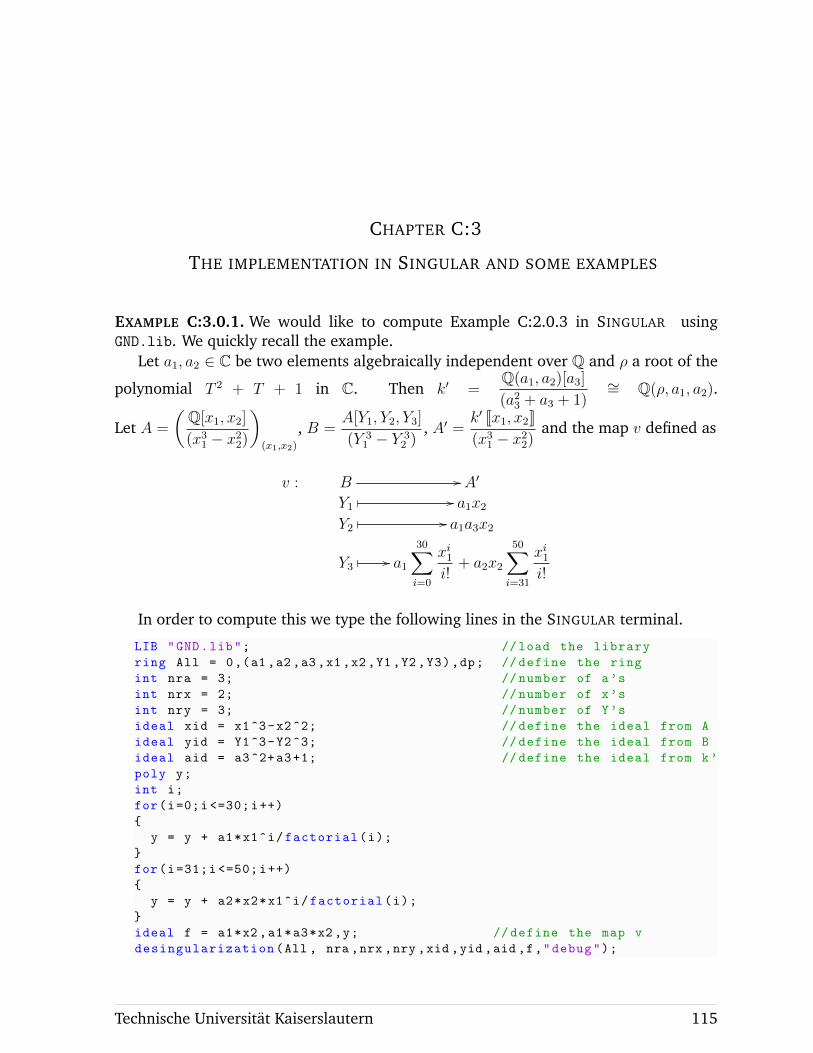
CHAPTER C:3
THE IMPLEMENTATION IN SINGULAR AND SOME EXAMPLES
EXAMPLE C:3.0.1. We would like to compute Example C:2.0.3 in SINGULAR usingGND.lib. We quickly recall the example.
Let a1, a2 ∈ C be two elements algebraically independent over Q and ρ a root of the
polynomial T 2 + T + 1 in C. Then k′ =Q(a1, a2)[a3]
(a23 + a3 + 1)∼= Q(ρ, a1, a2).
Let A =
(Q[x1, x2]
(x31 − x22)
)(x1,x2)
, B =A[Y1, Y2, Y3]
(Y 31 − Y 3
2 ), A′ =
k′ Jx1, x2K(x31 − x22)
and the map v defined as
v : B // A′
Y1� // a1x2
Y2� // a1a3x2
Y3� // a1
30∑i=0
xi1i!
+ a2x2
50∑i=31
xi1i!
In order to compute this we type the following lines in the SINGULAR terminal.
LIB "GND.lib"; //load the library
ring All = 0,(a1 ,a2 ,a3 ,x1 ,x2 ,Y1 ,Y2 ,Y3),dp; // define the ring
int nra = 3; // number of a’s
int nrx = 2; // number of x’s
int nry = 3; // number of Y’s
ideal xid = x1^3-x2^2; // define the ideal from A
ideal yid = Y1^3-Y2^3; // define the ideal from B
ideal aid = a3^2+a3+1; // define the ideal from k’
poly y;
int i;
for(i=0;i <=30;i++)
{
y = y + a1*x1^i/factorial(i);
}
for(i=31;i <=50;i++)
{
y = y + a2*x2*x1^i/factorial(i);
}
ideal f = a1*x2,a1*a3*x2,y; // define the map v
desingularization(All , nra ,nrx ,nry ,xid ,yid ,aid ,f,"debug");
Technische Universitat Kaiserslautern 115
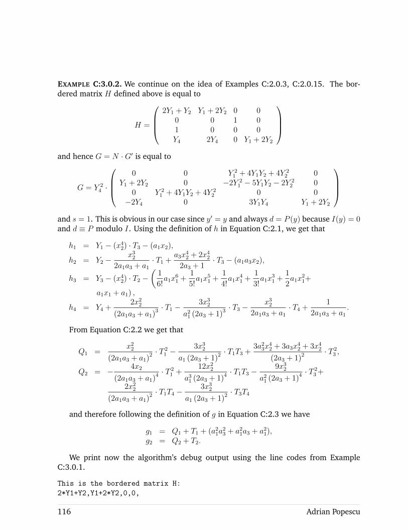
EXAMPLE C:3.0.2. We continue on the idea of Examples C:2.0.3, C:2.0.15. The bor-dered matrix H defined above is equal to
H =
2Y1 + Y2 Y1 + 2Y2 0 0
0 0 1 01 0 0 0Y4 2Y4 0 Y1 + 2Y2
and hence G = N ·G′ is equal to
G = Y 24 ·
0 0 Y 2
1 + 4Y1Y2 + 4Y 22 0
Y1 + 2Y2 0 −2Y 21 − 5Y1Y2 − 2Y 2
2 00 Y 2
1 + 4Y1Y2 + 4Y 22 0 0
−2Y4 0 3Y1Y4 Y1 + 2Y2
and s = 1. This is obvious in our case since y′ = y and always d = P (y) because I(y) = 0and d ≡ P modulo I. Using the definition of h in Equation C:2.1, we get that
h1 = Y1 − (x42) · T3 − (a1x2),
h2 = Y2 −x32
2a1a3 + a1· T1 +
a3x42 + 2x42
2a3 + 1· T3 − (a1a3x2),
h3 = Y3 − (x42) · T2 −(
1
6!a1x
61 +
1
5!a1x
51 +
1
4!a1x
41 +
1
3!a1x
31 +
1
2a1x
21+
a1x1 + a1) ,
h4 = Y4 +2x22
(2a1a3 + a1)3 · T1 −
3x32a21 (2a3 + 1)3
· T3 −x32
2a1a3 + a1· T4 +
1
2a1a3 + a1.
From Equation C:2.2 we get that
Q1 =x22
(2a1a3 + a1)2 · T
21 −
3x32a1 (2a3 + 1)2
· T1T3 +3a23x
42 + 3a3x
42 + 3x42
(2a3 + 1)2· T 2
3 ,
Q2 = − 4x2
(2a1a3 + a1)4 · T
21 +
12x22a31 (2a3 + 1)4
· T1T3 −9x32
a21 (2a3 + 1)4· T 2
3 +
2x22(2a1a3 + a1)
2 · T1T4 −3x32
a1 (2a3 + 1)2· T3T4
and therefore following the definition of g in Equation C:2.3 we have
g1 = Q1 + T1 + (a21a23 + a21a3 + a21),
g2 = Q2 + T2.
We print now the algorithm’s debug output using the line codes from ExampleC:3.0.1.
This is the bordered matrix H:
2*Y1+Y2,Y1+2*Y2,0,0,
116 Adrian Popescu
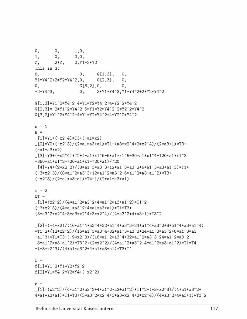
0, 0, 1,0,
1, 0, 0,0,
Z, 2*Z, 0,Y1+2*Y2
This is G:
0, 0, G[1,3], 0,
Y1*Y4^2+2*Y2*Y4^2,0, G[2,3], 0,
0, G[3,2],0, 0,
-2*Y4^3, 0, 3*Y1*Y4^3,Y1*Y4^2+2*Y2*Y4^2
G[1,3]=Y1^2*Y4^2+4*Y1*Y2*Y4^2+4*Y2^2*Y4^2
G[2,3]=-2*Y1^2*Y4^2-5*Y1*Y2*Y4^2-2*Y2^2*Y4^2
G[3,2]=Y1^2*Y4^2+4*Y1*Y2*Y4^2+4*Y2^2*Y4^2
s = 1
h =
_[1]=Y1+(-x2^4)*T3+(-a1*x2)
_[2]=Y2+(-x2^3)/(2*a1*a3+a1)*T1+(a3*x2^4+2*x2^4)/(2*a3+1)*T3+
(-a1*a3*x2)
_[3]=Y3+(-x2^4)*T2+(-a1*x1^6-6*a1*x1^5-30*a1*x1^4-120*a1*x1^3
-360*a1*x1^2-720*a1*x1-720*a1)/720
_[4]=Y4+(2*x2^2)/(8*a1^3*a3^3+12*a1^3*a3^2+6*a1^3*a3+a1^3)*T1+
(-3*x2^3)/(8*a1^2*a3^3+12*a1^2*a3^2+6*a1^2*a3+a1^2)*T3+
(-x2^3)/(2*a1*a3+a1)*T4-1/(2*a1*a3+a1)
m = 2
QT =
_[1]=(x2^2)/(4*a1^2*a3^2+4*a1^2*a3+a1^2)*T1^2+
(-3*x2^3)/(4*a1*a3^2+4*a1*a3+a1)*T1*T3+
(3*a3^2*x2^4+3*a3*x2^4+3*x2^4)/(4*a3^2+4*a3+1)*T3^2
_[2]=(-4*x2)/(16*a1^4*a3^4+32*a1^4*a3^3+24*a1^4*a3^2+8*a1^4*a3+a1^4)
*T1^2+(12*x2^2)/(16*a1^3*a3^4+32*a1^3*a3^3+24*a1^3*a3^2+8*a1^3*a3
+a1^3)*T1*T3+(-9*x2^3)/(16*a1^2*a3^4+32*a1^2*a3^3+24*a1^2*a3^2
+8*a1^2*a3+a1^2)*T3^2+(2*x2^2)/(4*a1^2*a3^2+4*a1^2*a3+a1^2)*T1*T4
+(-3*x2^3)/(4*a1*a3^2+4*a1*a3+a1)*T3*T4
f =
f[1]=Y1^2+Y1*Y2+Y2^2
f[2]=Y1*Y4+2*Y2*Y4+(-x2^2)
g =
_[1]=(x2^2)/(4*a1^2*a3^2+4*a1^2*a3+a1^2)*T1^2+(-3*x2^3)/(4*a1*a3^2+
4*a1*a3+a1)*T1*T3+(3*a3^2*x2^4+3*a3*x2^4+3*x2^4)/(4*a3^2+4*a3+1)*T3^2
Technische Universitat Kaiserslautern 117
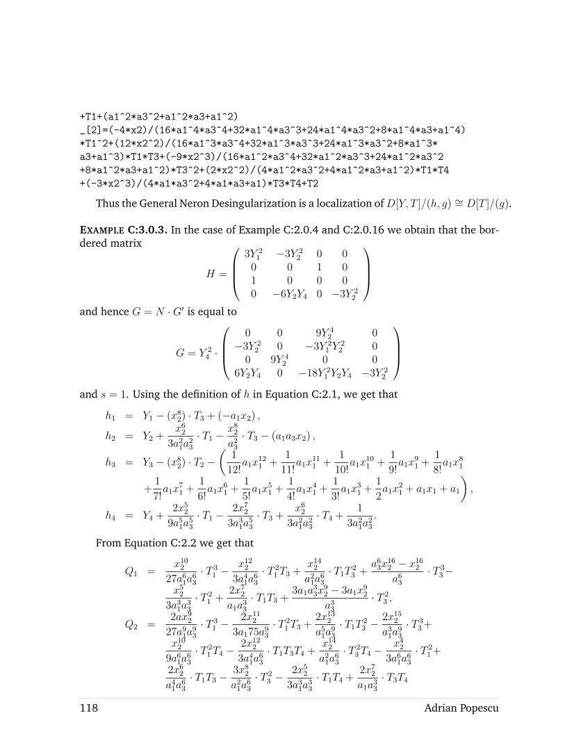
+T1+(a1^2*a3^2+a1^2*a3+a1^2)
_[2]=(-4*x2)/(16*a1^4*a3^4+32*a1^4*a3^3+24*a1^4*a3^2+8*a1^4*a3+a1^4)
*T1^2+(12*x2^2)/(16*a1^3*a3^4+32*a1^3*a3^3+24*a1^3*a3^2+8*a1^3*
a3+a1^3)*T1*T3+(-9*x2^3)/(16*a1^2*a3^4+32*a1^2*a3^3+24*a1^2*a3^2
+8*a1^2*a3+a1^2)*T3^2+(2*x2^2)/(4*a1^2*a3^2+4*a1^2*a3+a1^2)*T1*T4
+(-3*x2^3)/(4*a1*a3^2+4*a1*a3+a1)*T3*T4+T2
Thus the General Neron Desingularization is a localization ofD[Y, T ]/(h, g) ∼= D[T ]/(g).
EXAMPLE C:3.0.3. In the case of Example C:2.0.4 and C:2.0.16 we obtain that the bor-dered matrix
H =
3Y 2
1 −3Y 22 0 0
0 0 1 01 0 0 00 −6Y2Y4 0 −3Y 2
2
and hence G = N ·G′ is equal to
G = Y 24 ·
0 0 9Y 4
2 0−3Y 2
2 0 −3Y 21 Y
22 0
0 9Y 42 0 0
6Y2Y4 0 −18Y 21 Y2Y4 −3Y 2
2
and s = 1. Using the definition of h in Equation C:2.1, we get that
h1 = Y1 − (x82) · T3 + (−a1x2) ,
h2 = Y2 +x62
3a21a23
· T1 −x82a23· T3 − (a1a3x2) ,
h3 = Y3 − (x82) · T2 −(
1
12!a1x
121 +
1
11!a1x
111 +
1
10!a1x
101 +
1
9!a1x
91 +
1
8!a1x
81
+1
7!a1x
71 +
1
6!a1x
61 +
1
5!a1x
51 +
1
4!a1x
41 +
1
3!a1x
31 +
1
2a1x
21 + a1x1 + a1
),
h4 = Y4 +2x52
9a51a53
· T1 −2x72
3a31a53
· T3 +x62
3a21a23
· T4 +1
3a21a23
.
From Equation C:2.2 we get that
Q1 =x102
27a61a63
· T 31 −
x1223a41a
63
· T 21 T3 +
x142a21a
63
· T1T 23 +
a63x162 − x162a63
· T 33−
x523a31a
33
· T 21 +
2x72a1a33
· T1T3 +3a1a
33x
92 − 3a1x
92
a33· T 2
3 ,
Q2 =2ax92
27a91a93
· T 31 −
2x1123a175a93
· T 21 T3 +
2x132a51a
93
· T1T 23 −
2x152a31a
93
· T 33 +
x1029a61a
63
· T 21 T4 −
2x1223a41a
63
· T1T3T4 +x142a21a
63
· T 23 T4 −
x423a61a
63
· T 21 +
2x62a41a
63
· T1T3 −3x82a21a
63
· T 23 −
2x523a31a
33
· T1T4 +2x72a1a33
· T3T4
118 Adrian Popescu
and therefore following the definition of g in Equation C:2.3 we have
g1 = Q1 + T1,g2 = Q2 + T2
To obtain this with SINGULAR , we use the same code lines as in Example C:3.0.1,but we change the last one with
desingularization(All , nra ,nrx ,nry ,xid ,yid ,aid ,f,"injective","debug");
Doing this, the algorithm will not compute the kernel because of the “injective” argu-ment.
EXAMPLE C:3.0.4. We do now the same computations for Examples C:2.0.7 and C:2.0.17.The bordered matrix H is equal to
H =
x2 −x1 0 00 0 1 01 0 0 00 0 0 −x1x23
and hence G = N ·G′ is equal to
G = Y 24 ·
0 0 x21x
43 0
−x1x43 0 x1x2x43 0
0 x21x43 0 0
0 0 0 −x1x23
and s = 1. Using the definition of h in Equation C:2.1, we get that
h1 = Y1 + (x31x63) · T3 − (a3x1),
h2 = Y2 − (x21x63) · T1 + (x21x2x
63) · T3 − (a3x2),
h3 = Y3 + (x31x63) · T2 −
(1
7!a1x
73 +
1
6!a1x
63 +
1
5!a1x
53
+1
4!a1x
43 +
1
3!a1x
33 +
1
2!a1x
23 + a1x3 + a1
),
h4 = Y4 + (x21x43) · T4 + 1.
From Equation C:2.2 we obtain
Q1 = 0,Q2 = 0
and therefore following the definition of g in Equation C:2.3 we have
g1 = T1g2 = T2.
To compute this with the SINGULAR library we type the following in the terminal:
Technische Universitat Kaiserslautern 119
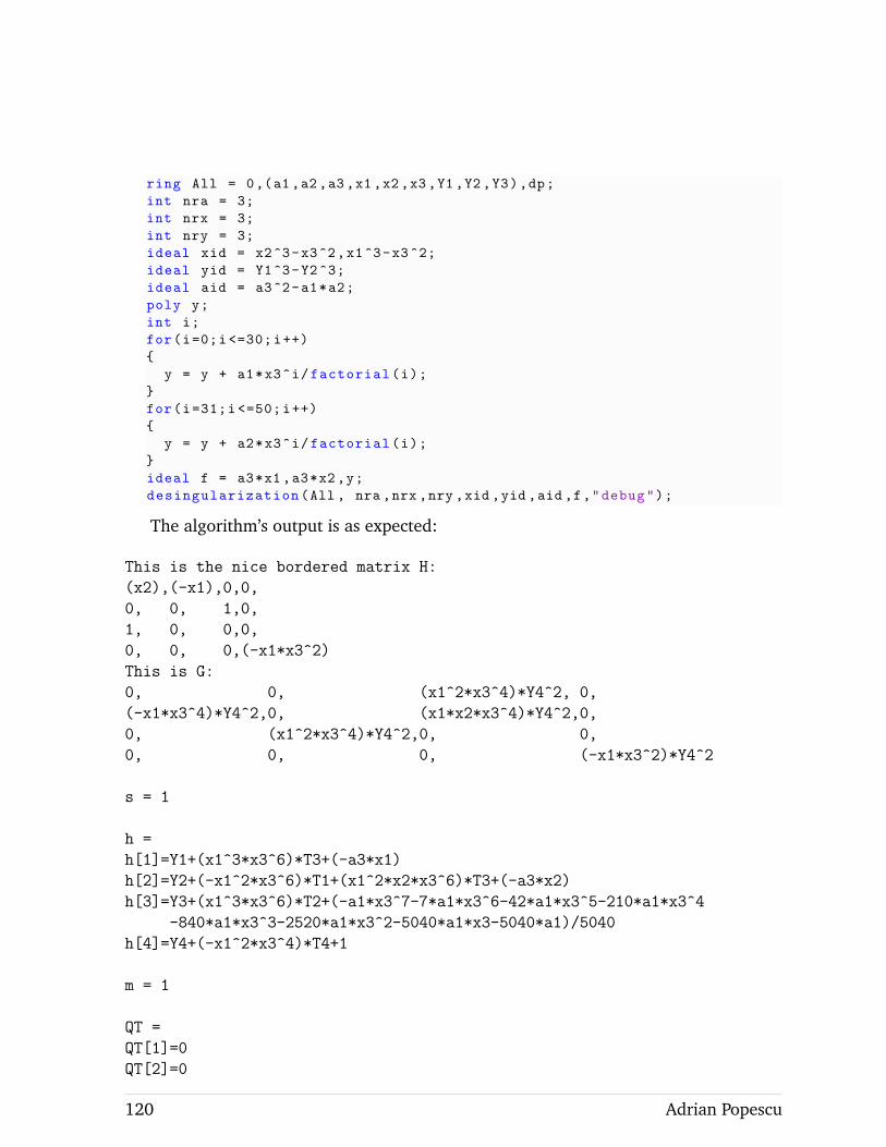
ring All = 0,(a1 ,a2 ,a3 ,x1 ,x2 ,x3 ,Y1 ,Y2 ,Y3),dp;
int nra = 3;
int nrx = 3;
int nry = 3;
ideal xid = x2^3-x3^2,x1^3-x3^2;
ideal yid = Y1^3-Y2^3;
ideal aid = a3^2-a1*a2;
poly y;
int i;
for(i=0;i <=30;i++)
{
y = y + a1*x3^i/factorial(i);
}
for(i=31;i <=50;i++)
{
y = y + a2*x3^i/factorial(i);
}
ideal f = a3*x1,a3*x2,y;
desingularization(All , nra ,nrx ,nry ,xid ,yid ,aid ,f,"debug");
The algorithm’s output is as expected:
This is the nice bordered matrix H:
(x2),(-x1),0,0,
0, 0, 1,0,
1, 0, 0,0,
0, 0, 0,(-x1*x3^2)
This is G:
0, 0, (x1^2*x3^4)*Y4^2, 0,
(-x1*x3^4)*Y4^2,0, (x1*x2*x3^4)*Y4^2,0,
0, (x1^2*x3^4)*Y4^2,0, 0,
0, 0, 0, (-x1*x3^2)*Y4^2
s = 1
h =
h[1]=Y1+(x1^3*x3^6)*T3+(-a3*x1)
h[2]=Y2+(-x1^2*x3^6)*T1+(x1^2*x2*x3^6)*T3+(-a3*x2)
h[3]=Y3+(x1^3*x3^6)*T2+(-a1*x3^7-7*a1*x3^6-42*a1*x3^5-210*a1*x3^4
-840*a1*x3^3-2520*a1*x3^2-5040*a1*x3-5040*a1)/5040
h[4]=Y4+(-x1^2*x3^4)*T4+1
m = 1
QT =
QT[1]=0
QT[2]=0
120 Adrian Popescu

f =
f[1]=(x2)*Y1+(-x1)*Y2
f[2]=(x1*x3^2)*Y4+(-x1*x3^2)
g
_[1]=T1
_[2]=T2
Thus the General Neron Desingularization is a localization of D[Y, T3, T4]/(h) ∼=D[T3, T4].
EXAMPLE C:3.0.5. We do now the same computations for Example C:2.0.18. In thisexample, the computations are much more complicated. The output is unfortunatelytoo big but we will try our best to describe the result.
The bordered matrix H is equal to
H =
0 x2 · Y3 x2 · Y2 −2 · Y4 0
x21 · Y2 x21 · Y1 −2 · Y3 0 00 1 0 0 01 0 0 0 00 0 4Y4Y5 4Y3Y5 4Y3Y4
and hence G = N ·G′ is equal to
G = Y 25 ·
0 0 0 16Y 2
3 Y24 0
0 0 16Y 23 Y
24 0 0
0 −8Y3Y24 8x21 · Y1Y3Y 2
4 8x21 · Y2Y3Y 24 0
−8Y 23 Y4 −4x2 · Y2Y3Y4 G[4, 3] 4x21x2 · Y 2
2 Y3Y4 08Y 2
3 Y5 x2 · Y2Y3Y5 + 2Y 24 Y5 G[5, 3] G[5, 4] 4Y3Y4
,
whereG[4, 3] = 4x21x2 · Y1Y2Y3Y4 + 2x2 · Y 3
3 Y4,G[5, 3] = −4x21x2 · Y1Y2Y3Y5 − 2x2 · Y 3
3 Y5 − 2x21 · Y1Y 24 Y5 and
G[5, 4] = −4x21x2 · Y 22 Y3Y5 − 2x21 · Y2Y 2
4 Y5
and
s = a81a22x
122 − 2a51a
42x
132 + a21a
62x
142 − 2a61a
32x
122 + 2a31a
52x
132 − a41a42x122 + 2a1a
62x
132 +
2a81a2x102 − 4a51a
32x
112 + 4a21a
52x
122 − 4a61a
22x
102 + 4a31a
42x
112 + a62x
122 + 2a1a
52x
112 +
a81x82 − 2a51a
22x
92 + 3a21a
42x
102 − 2a61a2x
82 + 2a31a
32x
92 + a41a
22x
82 − 2a41a2x
62+
2a1a32x
72 + 2a21a
22x
62 + 2a32x
62 − 2a41x
42 + 2a1a
22x
52 + 2a21a2x
42 + 1
Using the definition of h in Equation C:2.1, we get thath1h2h3h4h5
= s ·
Y1 − y′1Y2 − y′2Y3 − y′3Y4 − y′4Y5 − y′5
− x42G(y′) ·
T1T2T3T4T5
,
Technische Universitat Kaiserslautern 121
where
y′1 = −18a21a52x
122 + 5a31a
42x
112 + 7a62x
122 − 18a1a
52x
112 + 15a21a
42x
102 − 4a31a
32x
92−
6a52x102 + 15a1a
42x
92 − 12a21a
32x
82 + 3a31a
22x
72 + 5a42x
82 − 12a1a
32x
72 + 9a21a
22x
62−
2a31a2x52 − 4a32x
62 + 9a1a
22x
52 − 6a21a2x
42 + a31x
32 + 3a22x
42 − 6a1a2x
32 + 3a21x
22−
2a2x22 + 3a1x2 + 1
y′2 = a121 x122 + 2a101 a2x
122 − a111 x112 + a81a
22x
122 − 2a91a2x
112 + a101 x
102 − a71a22x112 +
2a81a2x102 − a91x92 + a61a
22x
102 − 2a71a2x
92 + a81x
82 − a51a22x92 + 2a61a2x
82 − a71x72+
a41a22x
82 − 2a51a2x
72 + a61x
62 − a31a22x72 + 2a41a2x
62 − a51x52 + a21a
22x
62 − 2a31a2x
52+
a41x42 − a1a22x52 + 2a21a2x
42 − a31x32 + a22x
42 − 2a1a2x
32 + a21x
22 + 2a2x
22 − a1x2+
1y′3 = a1x
22 + x2
y′4 = a2x32 + x2
y′5 =a224x42 −
a31 + a1a24
x32 +a21 − a2
4x22 −
a14x2 +
1
4.
However, the output is too big to be printed. Following the idea in the above exam-ples, we compute Q and g. This is even bigger than h so we print the numerators anddenominators of the coefficients just till degree 10 in the xi’s. However in some caseseven the terms till degree 10 will be too many to write down and hence we will printjust the first terms and “. . .” .
As a small remark, Q3 contains also terms in degree 3 in the Ti but the numeratorof the coefficients have power greater than 10 and therefore they do not appear in ourshort-cutting.
Q1 =3a21x
21x
82−2a1x21x72+4a2x21x
82+x
21x
62
4a1a22x52+8a1a2x32+4a1x2+4a22x
42+8a2x22+4
· T1T4 −x62
4a22x42+8a2x22+4
· T 21
+−a41x102 +a31x
92−2a21a2x102 −a21x82+2a1a2x92+a1x
72−a22x102 −2a2x82−x62
4a1a22x52+8a1a2x32+4a1x2+4a22x
42+8a2x22+4
· T1T2
+−5a41x102 +4a31x
92−12a21a2x102 −3a21x82+8a1a2x92+2a1x72−6a22x102 −4a2x82−x62
16a21a22x
62+32a21a2x
42+16a21x
22+32a1a22x
52+64a1a2x32+32a1x2+16a22x
42+32a2x22+16
· T 22
+a21x
21x
82+2a21x
102 +2a1x21x
72+4a1x92+x
21x
62+2x82
4a1a22x52+8a1a2x32+4a1x2+4a22x
42+8a2x22+4
· T1T3
+a1x21x
72−2a1x92+2a2x21x
82−4a2x102 +x21x
62−2x82
8a21a22x
62+16a21a2x
42+8a21x
22+16a1a22x
52+32a1a2x32+16a1x2+8a22x
42+16a2x22+8
· T2T3
+−x41x62+4x21x
82−4x10²
16a21a22x
62+32a21a2x
42+16a21x
22+32a1a22x
52+64a1a2x32+32a1x2+16a22x
42+32a2x22+16
· T 23
+6a21x
21x
82−3a1x21x72+6a2x21x
82+x
21x
62
8a21a22x
62+16a21a2x
42+8a21x
22+16a1a22x
52+32a1a2x32+16a1x2+8a22x
42+16a2x22+8
· T2T4
+−x41x62+2x21x
82
8a21a22x
62+16a21a2x
42+8a21x
22+16a1a22x
52+32a1a2x32+16a1x2+8a22x
42+16a2x22+8
· T3T4
122 Adrian Popescu
+−x41x62
16a21a22x
62+32a21a2x
42+16a21x
22+32a1a22x
52+64a1a2x32+32a1x2+16a22x
42+32a2x22+16
· T 24
Q2 =−x62
4a21x22+8a1x2+4
· T 22 +
3a21x21x
82+3a1x21x
72−2a2x21x82+x21x62
2a21x22+4a1x2+2
· T2T3 +−x41x62
4a21x22+8a1x2+4
· T 23
+a21x
21x
82−a1x21x72+2a2x21x
82+x
21x
62
2a21x22+4a1x2+2
· T2T4 +−x41x62+2x21x
82
2a21x22+4a1x2+2
· T3T4 +−x41x62
4a21x22+8a1x2+4
· T 24
Q3 =2a31x
92−4a21a2x102 −2a21x82+2a1a2x92+2a1x72−2a2x82−2x62
4a1a32x72+12a1a22x
52+12a1a2x32+4a1x2+4a32x
62+12a22x
42+12a2x22+4
· T1T2
+7a31x
92−28a21a2x102 −7a21x82+21a1a2x92+7a1x72−21a22x102 −21a2x82−7x62
...+48a21x22+48a1a32x
72+144a1a22x
52+144a1a2x32+48a1x2+16a32x
62+48a22x
42+48a2x22+16
· T 22
+2a21x
21x
82+2a21x
102 +4a1x21x
72+4a1x92−2a2x21x82−2a2x102 +2x21x
62+2x82
4a1a32x72+12a1a22x
52+12a1a2x32+4a1x2+4a32x
62+12a22x
42+12a2x22+4
· T1T3
+7a21x
21x
82+4a21x
102 +14a1x21x
72+8a1x92+7a2x21x
82+4a2x102 +7x21x
62+4x82
...+24a21x22+24a1a32x
72+72a1a22x
52+72a1a2x32+24a1x2+8a32x
62+24a22x
42+24a2x22+8
· T2T3
+−7x41x62−8x21x82−4x10²
...+48a21x22+48a1a32x
72+144a1a22x
52+144a1a2x32+48a1x2+16a32x
62+48a22x
42+48a2x22+16
· T 23
+6a21x
21x
82−4a1x21x72+6a2x21x
82+2x21x
62
4a1a32x72+12a1a22x
52+12a1a2x32+4a1x2+4a32x
62+12a22x
42+12a2x22+4
· T1T4
+21a21x
21x
82−14a1x21x72+35a2x21x
82+7x21x
62
...+24a21x22+24a1a32x
72+72a1a22x
52+72a1a2x32+24a1x2+8a32x
62+24a22x
42+24a2x22+8
· T2T4
+−7x41x62−4x21x82
...+24a21x22+24a1a32x
72+72a1a22x
52+72a1a2x32+24a1x2+8a32x
62+24a22x
42+24a2x22+8
· T3T4
+−7x41x62
...+48a21x22+48a1a32x
72+144a1a22x
52+144a1a2x32+48a1x2+16a32x
62+48a22x
42+48a2x22+16
· T 24
+a41x
102 −a21a2x102 −a22x102 +a2x82−x62
4a32x62+12a22x
42+12a2x22+4
· T 21 +
−x62
2a22x42+4a2x22+2
· T1T5
+−3a22x102 −6a2x82−3x62
4a21a22x
62+8a21a2x
42+4a21x
22+8a1a22x
52+16a1a2x32+8a1x2+4a22x
42+8a2x22+4
· T2T5
+9a21x
21x
82+6a21x
102 +9a1x21x
72+6a1x92+3x21x
62+2x82
4a21a22x
62+8a21a2x
42+4a21x
22+8a1a22x
52+16a1a2x32+8a1x2+4a22x
42+8a2x22+4
· T3T5
+3a21x
21x
82−3a1x21x72+12a2x21x
82+3x21x
62
4a21a22x
62+8a21a2x
42+4a21x
22+8a1a22x
52+16a1a2x32+8a1x2+4a22x
42+8a2x22+4
· T4T5
Technische Universitat Kaiserslautern 123
The denominators of the coefficients from Q are invertible in D because they followfrom θ′3 and θ′4 which are invertible in D. Thus Q ∈ D[T1, . . . , T5]. Having Qi we obtaingi:
g1 = Q1+(...−6a41x42+30a31a
32x
92+45a21a
42x
102 +6a21a
22x
62+6a21a2x
42+6a1a32x
72+6a1a22x
52+6a32x
62+1)·T1
g2 = Q2+(...−6a41x42+30a31a
32x
92+45a21a
42x
102 +6a21a
22x
62+6a21a2x
42+6a1a32x
72+6a1a22x
52+6a32x
62+1)·T2
+(...+6a61x
42−30a51a32x92−45a41a42x102 −6a41a22x62−6a41a2x42−6a31a32x72−6a31a22x52−6a21a32x62−a21
)g3 = Q3+
(...−6a41x42+30a31a
32x
92+45a21a
42x
102 +6a21a
22x
62+6a21a2x
42+6a1a32x
72+6a1a22x
52+6a32x
62+1)·T3
+(...+24a21a
52x
102 +18a21a
42x
82+a
21a
22x
42+a
21a2x
22+12a1a52x
92+a1a
32x
52+a1a
22x
32+6a62x
102 +a32x
42
).
The General Neron Desingularization is a localization of D[Y, T ]/(h, g). To computethis example with our SINGULAR library, we will need a function
invp(poly p, int bound,string param,string variab)
which computes computes the inverse of p till order bound in Q(param)[variab].The input for this example is the following:ring All = 0,(a1 ,a2 ,x1 ,x2 ,Y1 ,Y2 ,Y3 ,Y4),dp;
int nra = 2;
int nrx = 2;
int nry = 4;
ideal xid = x1^2-x2^3;
ideal yid = Y3^2-x1^2*Y1*Y2,Y4^2-x2*Y2*Y3;
ideal aid = 0;
poly y1 ,y2 ,y3 ,y4;
y3 = 1+a1*x2;
y4 = 1+a2*x2^2;
string as ,xs;
if(nra != 0)
{
as = string(var (1));
for( int i=2;i<=nra;i++)
{
as = as+","+string(var(i));
}
}
if(nrx !=0)
{
xs = string(var(nra +1));
for(int i=nra+2;i<=nra+nrx;i++)
{
xs = xs+","+string(var(i));
}
}
y1 = y3^3* invp(y4^2,12,as ,xs);
y2 = y4^2* invp(y3 ,12,as ,xs);
y3 = x2*y3;
y4 = x2*y4;
ideal f = y1,y2,y3,y4;
desingularization(All , nra ,nrx ,nry ,xid ,yid ,aid ,f,"injective","debug");
124 Adrian Popescu
REMARK C:3.0.6. If we restrict our present algorithm to the case when A′ is the comple-tion of A then we might get a faster algorithm using the idea of the proof of TheoremC:2.0.19. This algorithm could be useful in the arc frame.
Technische Universitat Kaiserslautern 125

APPENDIX
Technische Universitat Kaiserslautern 127

EXAMPLES USED IN PART A
Technische Universitat Kaiserslautern 129

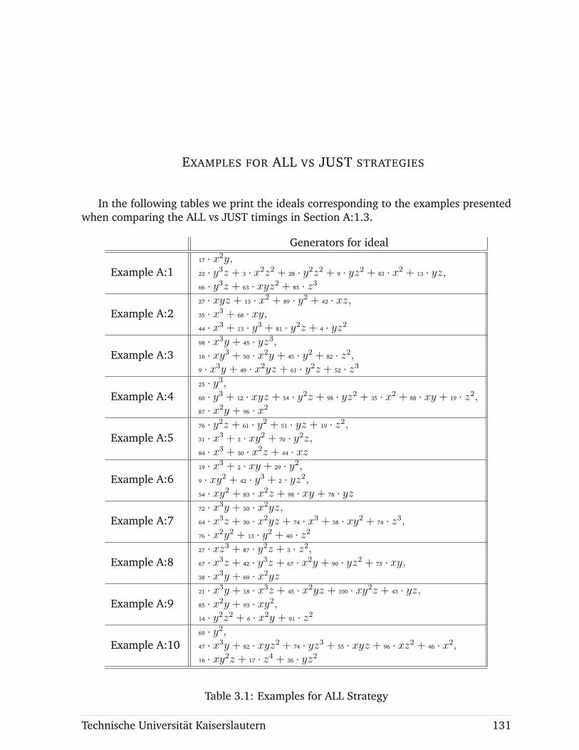
EXAMPLES FOR ALL VS JUST STRATEGIES
In the following tables we print the ideals corresponding to the examples presentedwhen comparing the ALL vs JUST timings in Section A:1.3.
Generators for ideal
Example A:117 · x2y,22 · y3z + 3 · x2z2 + 28 · y2z2 + 9 · yz2 + 83 · x2 + 13 · yz,66 · y3z + 63 · xyz2 + 85 · z3
Example A:227 · xyz + 13 · x2 + 89 · y2 + 42 · xz,35 · x3 + 68 · xy,44 · x3 + 13 · y3 + 81 · y2z + 4 · yz2
Example A:398 · x3y + 45 · yz3,16 · xy3 + 50 · x2y + 45 · y2 + 82 · z2,9 · x3y + 49 · x2yz + 61 · y2z + 52 · z3
Example A:425 · y3,60 · y3 + 12 · xyz + 54 · y2z + 98 · yz2 + 35 · x2 + 88 · xy + 19 · z2,87 · x2y + 96 · x2
Example A:576 · y2z + 61 · y2 + 51 · yz + 19 · z2,31 · x3 + 3 · xy2 + 70 · y2z,84 · x3 + 30 · x2z + 44 · xz
Example A:619 · x3 + 2 · xy + 29 · y2,9 · xy2 + 42 · y3 + 2 · yz2,54 · xy2 + 83 · x2z + 98 · xy + 78 · yz
Example A:772 · x3y + 50 · x2yz,64 · x3z + 30 · x2yz + 74 · x3 + 38 · xy2 + 74 · z3,76 · x2y2 + 13 · y2 + 40 · z2
Example A:827 · xz3 + 87 · y2z + 3 · z2,67 · x3z + 42 · y3z + 67 · x2y + 90 · yz2 + 73 · xy,38 · x3y + 69 · x2yz
Example A:921 · x3y + 18 · x3z + 45 · x2yz + 100 · xy2z + 43 · yz,85 · x2y + 93 · xy2,14 · y2z2 + 6 · x2y + 91 · z2
Example A:1069 · y2,47 · x3y + 82 · xyz2 + 74 · yz3 + 55 · xyz + 96 · xz2 + 46 · x2,16 · xy2z + 17 · z4 + 36 · yz2
Table 3.1: Examples for ALL Strategy
Technische Universitat Kaiserslautern 131
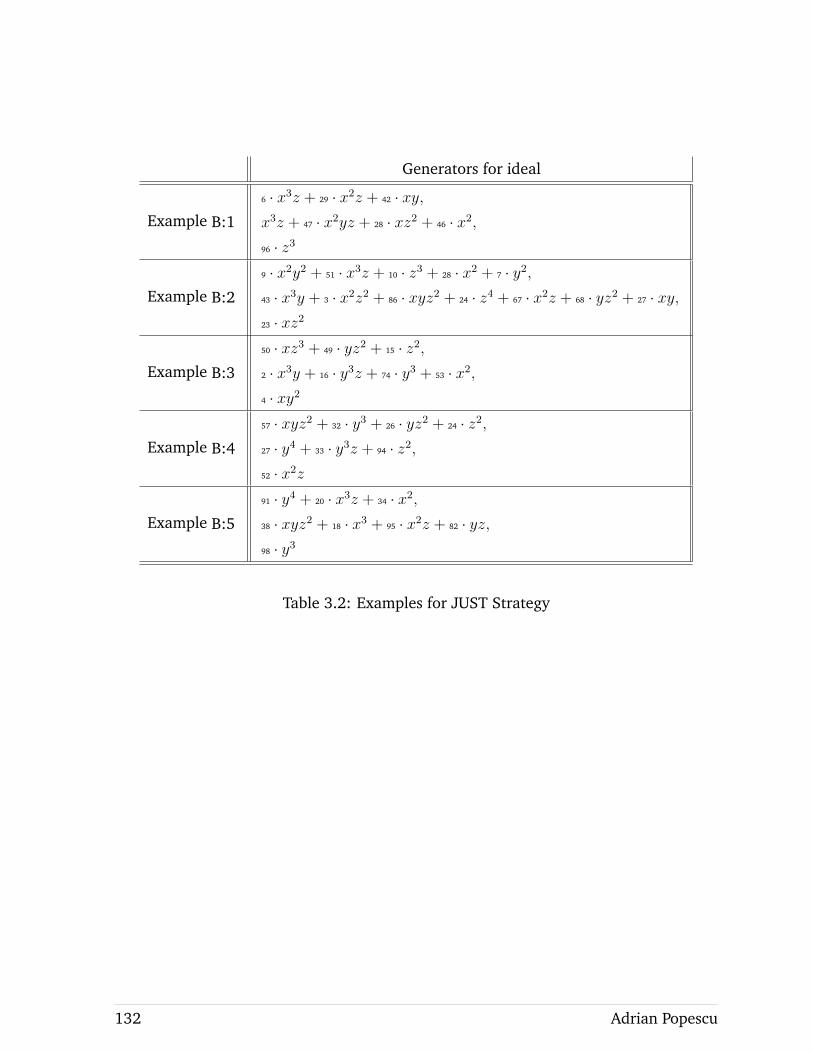
Generators for ideal
Example B:1
6 · x3z + 29 · x2z + 42 · xy,x3z + 47 · x2yz + 28 · xz2 + 46 · x2,96 · z3
Example B:2
9 · x2y2 + 51 · x3z + 10 · z3 + 28 · x2 + 7 · y2,43 · x3y + 3 · x2z2 + 86 · xyz2 + 24 · z4 + 67 · x2z + 68 · yz2 + 27 · xy,23 · xz2
Example B:3
50 · xz3 + 49 · yz2 + 15 · z2,2 · x3y + 16 · y3z + 74 · y3 + 53 · x2,4 · xy2
Example B:4
57 · xyz2 + 32 · y3 + 26 · yz2 + 24 · z2,27 · y4 + 33 · y3z + 94 · z2,52 · x2z
Example B:5
91 · y4 + 20 · x3z + 34 · x2,38 · xyz2 + 18 · x3 + 95 · x2z + 82 · yz,98 · y3
Table 3.2: Examples for JUST Strategy
132 Adrian Popescu
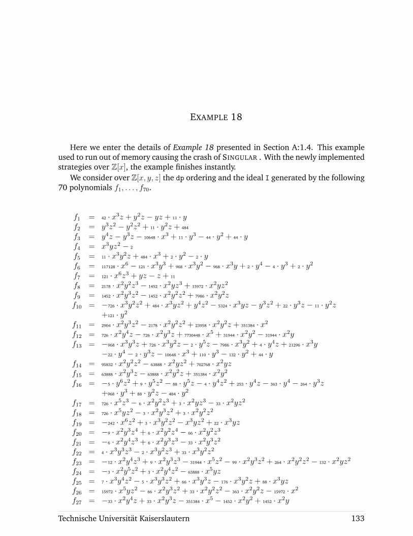
EXAMPLE 18
Here we enter the details of Example 18 presented in Section A:1.4. This exampleused to run out of memory causing the crash of SINGULAR . With the newly implementedstrategies over Z[x], the example finishes instantly.
We consider over Z[x, y, z] the dp ordering and the ideal I generated by the following70 polynomials f1, . . . , f70.
f1 = 42 · x3z + y2z − yz + 11 · yf2 = y3z2 − y2z2 + 11 · y2z + 484
f3 = y4z − y3z − 10648 · x3 + 11 · y3 − 44 · y2 + 44 · yf4 = x3yz2 − 2
f5 = 11 · x3y2z + 484 · x3 + 2 · y2 − 2 · yf6 = 117128 · x6 − 121 · x3y3 + 968 · x3y2 − 968 · x3y + 2 · y4 − 4 · y3 + 2 · y2f7 = 121 · x6z3 + yz − z + 11
f8 = 2178 · x2y2z3 − 1452 · x2yz3 + 15972 · x2yz2f9 = 1452 · x2y3z2 − 1452 · x2y2z2 + 7986 · x2y2zf10 = −726 · x3y2z2 + 484 · x3yz2 + y4z2 − 5324 · x3yz − y3z2 + 22 · y3z − 11 · y2z
+121 · y2f11 = 2904 · x2y3z2 − 2178 · x2y2z2 + 23958 · x2y2z + 351384 · x2f12 = 726 · x2y4z − 726 · x2y3z + 7730448 · x5 + 31944 · x2y2 − 31944 · x2yf13 = −968 · x3y3z + 726 · x3y2z − 2 · y5z − 7986 · x3y2 + 4 · y4z + 21296 · x3y
−22 · y4 − 2 · y3z − 10648 · x3 + 110 · y3 − 132 · y2 + 44 · yf14 = 95832 · x2y2z2 − 63888 · x2yz2 + 702768 · x2yzf15 = 63888 · x2y3z − 63888 · x2y2z + 351384 · x2y2f16 = −5 · y6z2 + 9 · y5z2 − 88 · y5z − 4 · y4z2 + 253 · y4z − 363 · y4 − 264 · y3z
+968 · y3 + 88 · y2z − 484 · y2f17 = 726 · x5z3 − 6 · x2y2z3 + 3 · x2yz3 − 33 · x2yz2f18 = 726 · x5yz2 − 3 · x2y3z2 + 3 · x2y2z2f19 = −242 · x6z2 + 3 · x3y2z2 − x3yz2 + 22 · x3yzf20 = −9 · x2y3z4 + 6 · x2y2z4 − 66 · x2y2z3f21 = −6 · x2y4z3 + 6 · x2y3z3 − 33 · x2y3z2f22 = 4 · x3y3z3 − 2 · x3y2z3 + 33 · x3y2z2f23 = −12 · x2y4z3 + 9 · x2y3z3 − 31944 · x5z2 − 99 · x2y3z2 + 264 · x2y2z2 − 132 · x2yz2f24 = −3 · x2y5z2 + 3 · x2y4z2 − 63888 · x5yzf25 = 7 · x3y4z2 − 5 · x3y3z2 + 66 · x3y3z − 176 · x3y2z + 88 · x3yzf26 = 15972 · x5yz2 − 66 · x2y3z2 + 33 · x2y2z2 − 363 · x2y2z − 15972 · x2f27 = −33 · x2y4z + 33 · x2y3z − 351384 · x5 − 1452 · x2y2 + 1452 · x2y
Technische Universitat Kaiserslautern 133
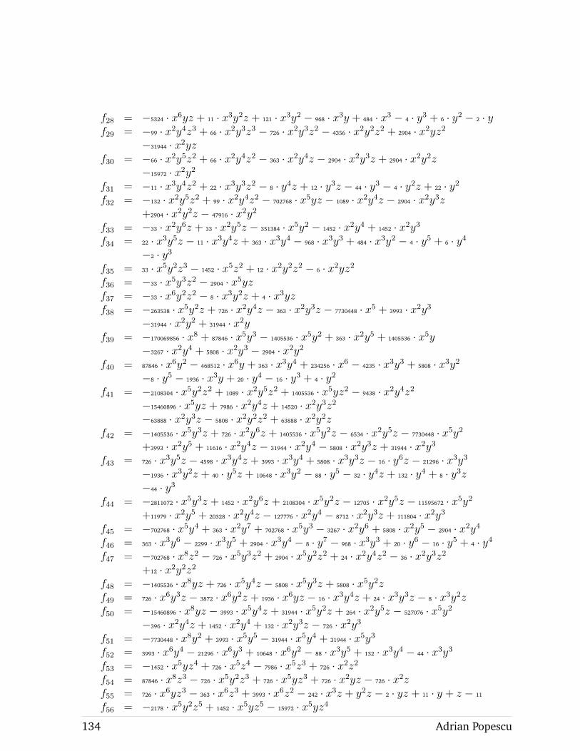
f28 = −5324 · x6yz + 11 · x3y2z + 121 · x3y2 − 968 · x3y + 484 · x3 − 4 · y3 + 6 · y2 − 2 · yf29 = −99 · x2y4z3 + 66 · x2y3z3 − 726 · x2y3z2 − 4356 · x2y2z2 + 2904 · x2yz2
−31944 · x2yzf30 = −66 · x2y5z2 + 66 · x2y4z2 − 363 · x2y4z − 2904 · x2y3z + 2904 · x2y2z
−15972 · x2y2f31 = −11 · x3y4z2 + 22 · x3y3z2 − 8 · y4z + 12 · y3z − 44 · y3 − 4 · y2z + 22 · y2f32 = −132 · x2y5z2 + 99 · x2y4z2 − 702768 · x5yz − 1089 · x2y4z − 2904 · x2y3z
+2904 · x2y2z − 47916 · x2y2f33 = −33 · x2y6z + 33 · x2y5z − 351384 · x5y2 − 1452 · x2y4 + 1452 · x2y3f34 = 22 · x3y5z − 11 · x3y4z + 363 · x3y4 − 968 · x3y3 + 484 · x3y2 − 4 · y5 + 6 · y4
−2 · y3f35 = 33 · x5y2z3 − 1452 · x5z2 + 12 · x2y2z2 − 6 · x2yz2f36 = −33 · x5y3z2 − 2904 · x5yzf37 = −33 · x6y2z2 − 8 · x3y2z + 4 · x3yzf38 = −263538 · x5y2z + 726 · x2y4z − 363 · x2y3z − 7730448 · x5 + 3993 · x2y3
−31944 · x2y2 + 31944 · x2yf39 = −170069856 · x8 + 87846 · x5y3 − 1405536 · x5y2 + 363 · x2y5 + 1405536 · x5y
−3267 · x2y4 + 5808 · x2y3 − 2904 · x2y2f40 = 87846 · x6y2 − 468512 · x6y + 363 · x3y4 + 234256 · x6 − 4235 · x3y3 + 5808 · x3y2
−8 · y5 − 1936 · x3y + 20 · y4 − 16 · y3 + 4 · y2f41 = −2108304 · x5y2z2 + 1089 · x2y5z2 + 1405536 · x5yz2 − 9438 · x2y4z2
−15460896 · x5yz + 7986 · x2y4z + 14520 · x2y3z2−63888 · x2y3z − 5808 · x2y2z2 + 63888 · x2y2z
f42 = −1405536 · x5y3z + 726 · x2y6z + 1405536 · x5y2z − 6534 · x2y5z − 7730448 · x5y2+3993 · x2y5 + 11616 · x2y4z − 31944 · x2y4 − 5808 · x2y3z + 31944 · x2y3
f43 = 726 · x3y5z − 4598 · x3y4z + 3993 · x3y4 + 5808 · x3y3z − 16 · y6z − 21296 · x3y3−1936 · x3y2z + 40 · y5z + 10648 · x3y2 − 88 · y5 − 32 · y4z + 132 · y4 + 8 · y3z−44 · y3
f44 = −2811072 · x5y3z + 1452 · x2y6z + 2108304 · x5y2z − 12705 · x2y5z − 11595672 · x5y2+11979 · x2y5 + 20328 · x2y4z − 127776 · x2y4 − 8712 · x2y3z + 111804 · x2y3
f45 = −702768 · x5y4 + 363 · x2y7 + 702768 · x5y3 − 3267 · x2y6 + 5808 · x2y5 − 2904 · x2y4f46 = 363 · x3y6 − 2299 · x3y5 + 2904 · x3y4 − 8 · y7 − 968 · x3y3 + 20 · y6 − 16 · y5 + 4 · y4f47 = −702768 · x8z2 − 726 · x5y3z2 + 2904 · x5y2z2 + 24 · x2y4z2 − 36 · x2y3z2
+12 · x2y2z2f48 = −1405536 · x8yz + 726 · x5y4z − 5808 · x5y3z + 5808 · x5y2zf49 = 726 · x6y3z − 3872 · x6y2z + 1936 · x6yz − 16 · x3y4z + 24 · x3y3z − 8 · x3y2zf50 = −15460896 · x8yz − 3993 · x5y4z + 31944 · x5y2z + 264 · x2y5z − 527076 · x5y2
−396 · x2y4z + 1452 · x2y4 + 132 · x2y3z − 726 · x2y3f51 = −7730448 · x8y2 + 3993 · x5y5 − 31944 · x5y4 + 31944 · x5y3f52 = 3993 · x6y4 − 21296 · x6y3 + 10648 · x6y2 − 88 · x3y5 + 132 · x3y4 − 44 · x3y3f53 = −1452 · x5yz4 + 726 · x5z4 − 7986 · x5z3 + 726 · x2z2f54 = 87846 · x8z3 − 726 · x5y2z3 + 726 · x5yz3 + 726 · x2yz − 726 · x2zf55 = 726 · x6yz3 − 363 · x6z3 + 3993 · x6z2 − 242 · x3z + y2z − 2 · yz + 11 · y + z − 11
f56 = −2178 · x5y2z5 + 1452 · x5yz5 − 15972 · x5yz4
134 Adrian Popescu
f57 = −1452 · x5y3z4 + 1452 · x5y2z4 − 7986 · x5y2z3f58 = 1089 · x6y2z4 − 726 · x6yz4 + 7986 · x6yz3 + y3z2 − 3 · y2z2 + 11 · y2z + 2 · yz2
−22 · yzf59 = −2904 · x5y3z4 + 2178 · x5y2z4 − 23958 · x5y2z3 + 63888 · x5yz3 − 31944 · x5z3
−31944 · x2zf60 = −726 · x5y4z3 + 726 · x5y3z3 − 11595672 · x8z2 − 31944 · x2y + 31944 · x2f61 = 1452 · x6y3z3 − 1089 · x6y2z3 + 11979 · x6y2z2 − 31944 · x6yz2 + 15972 · x6z2
+3 · y4z − 6 · y3z + 33 · y3 + 3 · y2z − 121 · y2 + 132 · y − 44
f62 = −726 · x8z5 + 3 · x2yz3f63 = −363 · x8yz4 + 3 · x2y2z2 − 3 · x2yz2f64 = 363 · x9z4 − x3yz2 − x3z2f65 = −15972 · x8yz4 − 2904 · x5yz3 + 1452 · x5z3 + 33 · x2y2z2 + 1452 · x2zf66 = 3993 · x8y2z3 + 527076 · x8z2 + 33 · x2y3z − 33 · x2y2z + 1452 · x2y − 1452 · x2f67 = 7986 · x9yz3 + 1452 · x6yz2 − 726 · x6z2 + 11 · x3y2z − 22 · x3yz + 4 · y2 − 6 · y + 2
f68 = 263538 · x8y2z3 − 1405536 · x8yz3 + 702768 · x8z3 − 5808 · x5y3z3 + 8712 · x5y2z3−2904 · x5yz3 + 702768 · x5z − 363 · x2y3z + 2904 · x2y2z − 2904 · x2yz
f69 = 255104784 · x11z2 − 131769 · x8y3z2 + 1054152 · x8y2z2 − 1054152 · x8yz2+702768 · x5y − 363 · x2y4 − 702768 · x5 + 3267 · x2y3 − 5808 · x2y2 + 2904 · x2y
f70 = −131769 · x9y2z2 + 702768 · x9yz2 − 351384 · x9z2 + 2904 · x6y3z2 − 4356 · x6y2z2+1452 · x6yz2 − 363 · x3y3 + 2299 · x3y2 − 2904 · x3y + 8 · y4 + 968 · x3 − 20 · y3+16 · y2 − 4 · y
Despite of how complicated the ideal I seems to be, its standard basis consists of fewsmall polynomials. We print below the result using SINGULAR .
ring r = integer ,(x,y,z),dp;
ideal I = ...;
std(I);
//>_[1]=18
//>_[2]=6z-12
//>_[3]=2y-4
//>_[4]=2 z2+4z+8
//>_[5]=yz+z+3
//>_[6]=3x2z -15x2
//>_[7]= x2y+3x2z+x2
//>_[8]=x3+10z
//>_[9]=x2z2 -4x2z -11x2
Using the new strategy described in Algorithm A:1.4.1, we compute the standardbasis over Q[x, y, z] and see that it is equal to 〈1〉. Hence the ideal contains a constant.Using SINGULAR ’s syzygy procedure syz, we are not lucky enough to already get ac-cess to 18, but a multiple of it: 6 133 248. This seems to be a big number, but if weadd this constant to the generators of I the computations will drastically speed up thecomputations.
We show how 6 133 248 can be generated using f1, . . . , f70.
Technische Universitat Kaiserslautern 135
6 133 248 = (−231913440x6z + 9838752x3y − 4599936x3z + 69696y) · f1+(−1584y3 + 13464y2 + 12672y)·f2+
(−115956720x6z + 1756920x3y − 1724976x3z − 40409160x3 + 52272y + 200376)·f3+(−38652240x3y3 + 38652240x3y2 + 154608960x3 + 1149984y2 + 4983264y + 3066624)·f4+
(−2551047840x6z + 38652240x3y − 37949472x3z − 889001520x3 + 574992y + 2779128)·f5+(−159720x3y2 − 159720x3y − 319440x3 − 2376y2 − 10296y − 12672)·f10+
(−79860x4 + 110xy3 + 110xy2 + 220xy − 2508x)·f11+(26136)·f13+
(3630x4y2 + 3630x4y + 7260x4 + 54xy2 + 154xy + 96x)·f14+(1540xy + 517x)·f15+
(−792)·f16+(425920x)·f18+
(−115956720x3y2 − 115956720x3y − 231913440x3 − 1724976y2 − 7474896y − 4599936)·f19+(−1756920x4 + 2420xy3 + 2420xy2 + 4840xy − 132616x)·f26+
(851840x)·f27+(287496)·f28+
(−38720x)·f38
136 Adrian Popescu
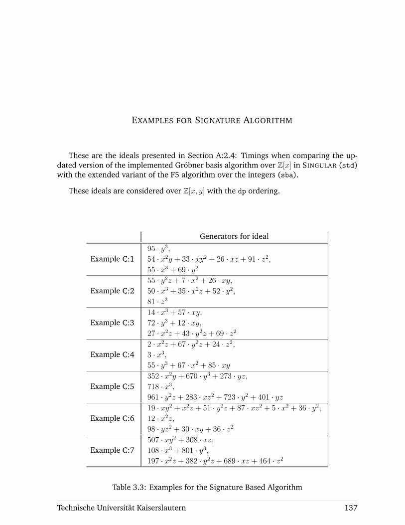
EXAMPLES FOR SIGNATURE ALGORITHM
These are the ideals presented in Section A:2.4: Timings when comparing the up-dated version of the implemented Grobner basis algorithm over Z[x] in SINGULAR (std)with the extended variant of the F5 algorithm over the integers (sba).
These ideals are considered over Z[x, y] with the dp ordering.
Generators for ideal
Example C:195 · y3,54 · x2y + 33 · xy2 + 26 · xz + 91 · z2,55 · x3 + 69 · y2
Example C:255 · y2z + 7 · x2 + 26 · xy,50 · x3 + 35 · x2z + 52 · y2,81 · z3
Example C:314 · x3 + 57 · xy,72 · y3 + 12 · xy,27 · x2z + 43 · y2z + 69 · z2
Example C:42 · x2z + 67 · y2z + 24 · z2,3 · x3,55 · y3 + 67 · x2 + 85 · xy
Example C:5352 · x2y + 670 · y3 + 273 · yz,718 · x3,961 · y2z + 283 · xz2 + 723 · y2 + 401 · yz
Example C:619 · xy2 + x2z + 51 · y2z + 87 · xz2 + 5 · x2 + 36 · y2,12 · x2z,98 · yz2 + 30 · xy + 36 · z2
Example C:7507 · xy2 + 308 · xz,108 · x3 + 801 · y3,197 · x2z + 382 · y2z + 689 · xz + 464 · z2
Table 3.3: Examples for the Signature Based Algorithm
Technische Universitat Kaiserslautern 137
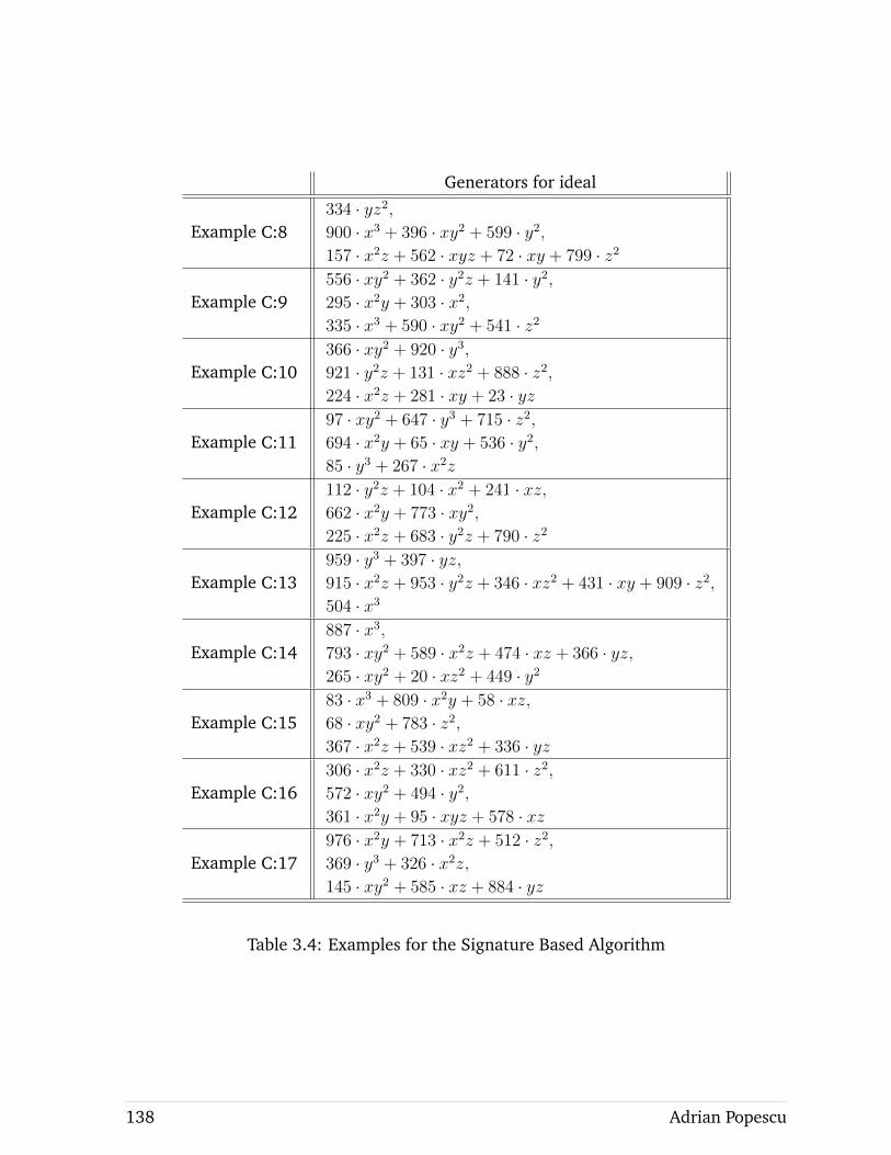
Generators for ideal
Example C:8334 · yz2,900 · x3 + 396 · xy2 + 599 · y2,157 · x2z + 562 · xyz + 72 · xy + 799 · z2
Example C:9556 · xy2 + 362 · y2z + 141 · y2,295 · x2y + 303 · x2,335 · x3 + 590 · xy2 + 541 · z2
Example C:10366 · xy2 + 920 · y3,921 · y2z + 131 · xz2 + 888 · z2,224 · x2z + 281 · xy + 23 · yz
Example C:1197 · xy2 + 647 · y3 + 715 · z2,694 · x2y + 65 · xy + 536 · y2,85 · y3 + 267 · x2z
Example C:12112 · y2z + 104 · x2 + 241 · xz,662 · x2y + 773 · xy2,225 · x2z + 683 · y2z + 790 · z2
Example C:13959 · y3 + 397 · yz,915 · x2z + 953 · y2z + 346 · xz2 + 431 · xy + 909 · z2,504 · x3
Example C:14887 · x3,793 · xy2 + 589 · x2z + 474 · xz + 366 · yz,265 · xy2 + 20 · xz2 + 449 · y2
Example C:1583 · x3 + 809 · x2y + 58 · xz,68 · xy2 + 783 · z2,367 · x2z + 539 · xz2 + 336 · yz
Example C:16306 · x2z + 330 · xz2 + 611 · z2,572 · xy2 + 494 · y2,361 · x2y + 95 · xyz + 578 · xz
Example C:17976 · x2y + 713 · x2z + 512 · z2,369 · y3 + 326 · x2z,145 · xy2 + 585 · xz + 884 · yz
Table 3.4: Examples for the Signature Based Algorithm
138 Adrian Popescu

Technische Universitat Kaiserslautern 139

PROGRAMMING IN SINGULAR ’S KERNEL
Technische Universitat Kaiserslautern 141

INTRODUCTION
SINGULAR is a computer algebra system for polynomial computations that has beendeveloped to help the users in various fields of mathematics like algebraic geometry,singularity theory and commutative algebra. It is a free software (GNU Public license)and it was supported by Deutsche Forschungsgemeinschaft (DFG), Stiftung Rheinland-Pfalz for Innovation and Volkswagen Stiftung.
The idea of SINGULAR began in 1984 when computing invariants of ideals and mod-ules in local rings (like Milnor, Tjurina numbers and dimensions) was needed to answerthe following question: Do there exist non-quasi homogeneous and complete intersectionsingularities with exact Poincare complex? The first step was to create a polynomial ringenvironment and implement a Grobner basis algorithm to make use of its properties.This first version was written in basic on a 8-bit ZX Spectrum machine. Shortly after,these where implemented for Atari using Modula-2 language and SINGULAR was born.In 1993 the code was rewritten in C-language.
In the first version of SINGULAR (1997), one could compute multivariate polyno-mial factorization, gcd, syzygies and resolutions. In the following year, version 1.2 wasreleased with faster algorithms, procedures for primary decompositions and normal-ization. Version 1.3 was again optimized, numerical data types and algorithms wereadded and one could compute moduli of space curves. SINGULAR 2.0 was released inthe early 2000’s and the textbook A Singular Introduction to Commutative Algebra waspublished as both an introduction to the software and to commutative algebra. Thebook has many examples on how to use computer algebra techniques in algebraic ge-ometry, commutative algebra and more. In 2004 at the International Symposium onSymbolic and Algebraic Computation (ISSAC), the SINGULAR team was awarded theRichard D. Jenks Memorial Prize for Excellence in Software Engineering for ComputerAlgebra. A couple of years later, a second enhanced edition of the Textbook was pub-lished containing more examples and accompanied by the release of SINGULAR 3.0,where non-commutative computations were possible together with absolute factoriza-tion and dynamic modules.
In the past 30+ years many developers worked on improving the algorithms, addingfeatures and building new libraries. At the moment the source code contains 9 663 files(in total more than 1 million code lines) and 145 libraries and it can get really hard tostart working in the sources.
This part will provide the reader with some basic guidelines into programming inSINGULAR ’s kernel, especially the part of the kernel specialized in the standard basescomputation (the so-called GBEngine).
Technische Universitat Kaiserslautern 143
THE STRUCTURE
The first chapter consists of the requirements needed to program in SINGULAR ’s ker-nel and explains some very basic concepts like git, compiling and building SINGULAR .
The second chapter introduces the main structures in the sources like polynomialsand ideals and lists the main related procedures pertaining to these concepts, e.g addingtwo polynomials, searching for constants in ideals, etc.
The third chapter explores the connection between the SINGULAR language is andthe internal structures.
The last chapter describes the adding of new structures and features to SINGULAR
while providing several examples.
144 Adrian Popescu
GIT, COMPILATION AND BUILDING
This section introduces the reader to the building of SINGULAR from the source files.A more detailed tutorial can be found on the Singular’s GitHub Wiki page. This is by nomeans a Git tutorial, the purpose is to obtain some insight into the methods and toolsused to develop SINGULAR .
In order to maintain a software as vast as SINGULAR , a large number of developersis required and it is vital that everybody works on the latest version. A problem mayoccur when two persons (say DevA and DevB) work on the same file in parallel. Thisleads to two versions of the file (say fileA and fileB). If the two developers wish to maketheir changes public, the the following scenario may happen: DevA will replace the oldfile with fileA. DevB will be unable to do the same since in this way DevA’s changes willbe lost. Hence DevB will have to change fileA manually.
Git is a free (version control) software that helps in this process. If the same linesof code were modified, a conflict appears and the code needs to be reviewed by one ofthe developers. Otherwise the merge is done automatically. In addition to this git alsoprovides the entire history of commits in order to help identifying the commit to blamewhen tests fail. A web version of Git with graphic interface, community and other usefultools can be found on GitHub.
In order to install SINGULAR on a Linux machine, certain prerequisites are needed.The complete list of software that one needs to install can be found atgithub.com/Singular/Sources/wiki/Step-by-Step-Installation-Instructions-for-Singular ,but the main ones are:
◦ git − version control,
◦ gcc − C++ compiler,
◦ automake − tool for generating compliant makefiles,
◦ autoconf − automatic configure script builder,
◦ make − utility for directing compilation,
◦ readline,
◦ GMP − multiprecission integer library (https://gmplib.org/)
◦ NTL− high-performance C++ library providing data structures and algorithms formanipulating arbitrary length integers, vectors, matrices, and polynomials overthe integers and over finite fields.
Technische Universitat Kaiserslautern 145
SINGULAR can be found as a Git repository at https://github.com/Singular/Sources.In order to implement some changes, first one needs to clone the repository locally, forexample in the Tutorial folder. This can be done by using the following command linein the Linux terminal:
git clone https :// github.com/Singular/Sources Tutorial
and generate the configure script using
cd Tutorial
./ autogen.sh
The most common way to configure and build SINGULAR is to run
./ configure
make
Now the program binary can be found in Tutorial/Singular/Singular.Sometimes a debug version is required − it is slightly slower, but sets debug flags
and therefore in case of a segmentation fault one can identify the file and line numberwhere it crashed using the debugger gdb’s backtrace command bt.
One can build a debug version by typing
./ configure --enable -debug --disable -optimizationflags
make
Since building SINGULAR is time consuming, it is recommended to use differentfolders for the various versions. Otherwise, the rebuilt of the entire software insteadof only parts of it will be required. In the following example we configure and buildSINGULAR in another folder, say Tutorial/Folder.
cd Tutorial
#creates a new folder
mkdir Folder
#changes the current working directory
cd Folder
#configures using the sources in Tutorial
../ configure
#builds Singular in parallel using 3 processors
make -j3
This newly build version of Singular can be found as the pathTutorial/Folder/Singular/Singular.
The repository can be viewed as a tree, the main branch is called spielwiese. In orderto modify it, a copy needs to be downloaded into the local machine and merged againto the main branch sometimes in the future. Note that this branch could have evolvedin the meantime. To avoid name confusion a new branch say (Changes) starting fromthe old one needs to be created. One can do this by typing
git checkout -b Changes
After the changes are commited (can be several commits, call them (C1), (C2), . . . ,(Cn)), the tree would look like this:
146 Adrian Popescu
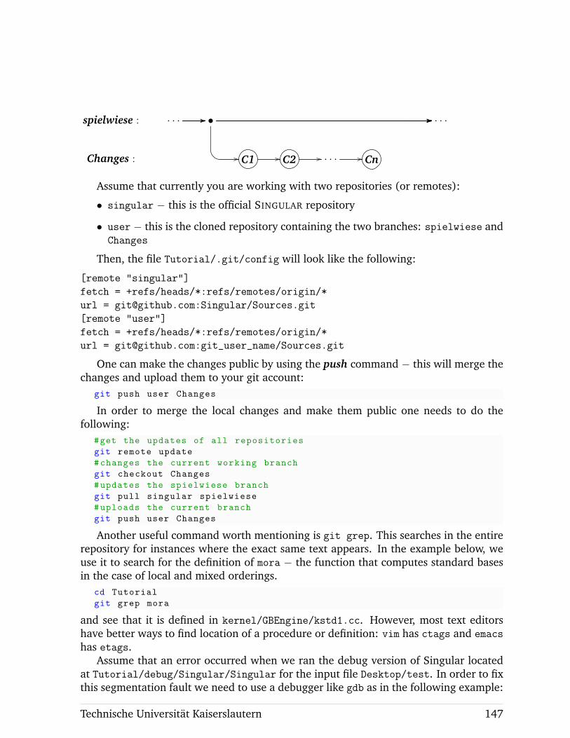
spielwiese : · · · ////// • //////
//
////// · · ·
Changes : C1 // C2 // · · · // Cn
Assume that currently you are working with two repositories (or remotes):
• singular − this is the official SINGULAR repository
• user − this is the cloned repository containing the two branches: spielwiese andChanges
Then, the file Tutorial/.git/config will look like the following:
[remote "singular"]
fetch = +refs/heads/*:refs/remotes/origin/*
url = [email protected]:Singular/Sources.git
[remote "user"]
fetch = +refs/heads/*:refs/remotes/origin/*
url = [email protected]:git_user_name/Sources.git
One can make the changes public by using the push command − this will merge thechanges and upload them to your git account:
git push user Changes
In order to merge the local changes and make them public one needs to do thefollowing:
#get the updates of all repositories
git remote update
#changes the current working branch
git checkout Changes
#updates the spielwiese branch
git pull singular spielwiese
#uploads the current branch
git push user Changes
Another useful command worth mentioning is git grep. This searches in the entirerepository for instances where the exact same text appears. In the example below, weuse it to search for the definition of mora − the function that computes standard basesin the case of local and mixed orderings.
cd Tutorial
git grep mora
and see that it is defined in kernel/GBEngine/kstd1.cc. However, most text editorshave better ways to find location of a procedure or definition: vim has ctags and emacs
has etags.Assume that an error occurred when we ran the debug version of Singular located
at Tutorial/debug/Singular/Singular for the input file Desktop/test. In order to fixthis segmentation fault we need to use a debugger like gdb as in the following example:
Technische Universitat Kaiserslautern 147
# starts debugging the binary
gdb Tutorial/debug/Singular/Singular
#run the program using as input the test file
r ~/ Desktop/test
When it breaks at the segmentation fault that caused SINGULAR to crash, one canbacktrace to find the cause of this error by typing bt. Adding breakpoints is useful whendebugging:
# creates a breakpoint in file GBEngine/kutil.cc. line 413
b kutil.cc:413
# creates a breakpoint at each call to the function redRing
b redRing
After a breakpoint, one can type the following:
step (or s) will go to the next line of code, will step in functions as wellnext (or n) will execute the next line of code, will not enter functionsfinish (or fin) will continue till the end of the current functioncontinue (or c) will continue till the next breakpoint
148 Adrian Popescu
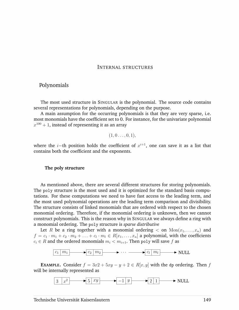
INTERNAL STRUCTURES
Polynomials
The most used structure in SINGULAR is the polynomial. The source code containsseveral representations for polynomials, depending on the purpose.
A main assumption for the occurring polynomials is that they are very sparse, i.e.most monomials have the coefficient set to 0. For instance, for the univariate polynomialx100 + 1, instead of representing it as an array
(1, 0 . . . , 0, 1),
where the i−th position holds the coefficient of xi+1, one can save it as a list thatcontains both the coefficient and the exponents.
The poly structure
As mentioned above, there are several different structures for storing polynomials.The poly structure is the most used and it is optimized for the standard basis compu-tations. For these computations we need to have fast access to the leading term, andthe most used polynomial operations are the leading term comparison and divisibility.The structure consists of linked monomials that are ordered with respect to the chosenmonomial ordering. Therefore, if the monomial ordering is unknown, then we cannotconstruct polynomials. This is the reason why in SINGULAR we always define a ring witha monomial ordering. The poly structure is sparse distributive
Let R be a ring together with a monomial ordering < on Mon(x1, . . . , xn) andf = c1 · m1 + c2 · m2 + . . . + cl · ml ∈ R[x1, . . . , xn] a polynomial, with the coefficientsci ∈ R and the ordered monomials mi < mi+1. Then poly will save f as
c1 m1 c2 m2 · · · cl ml NULL
EXAMPLE. Consider f = 3x2 + 5xy − y + 2 ∈ R[x, y] with the dp ordering. Then fwill be internally represented as
3 x2 5 xy −1 y 2 1 NULL
Technische Universitat Kaiserslautern 149
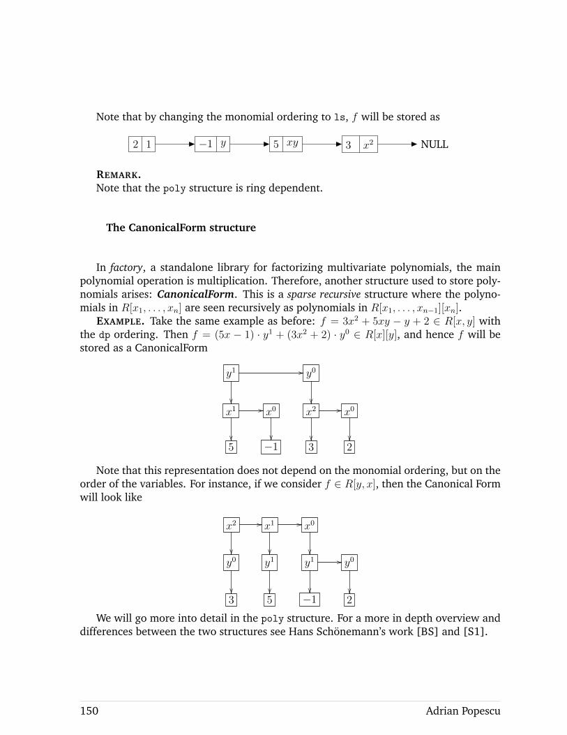
Note that by changing the monomial ordering to ls, f will be stored as
2 1 −1 y 5 xy 3 x2 NULL
REMARK.Note that the poly structure is ring dependent.
The CanonicalForm structure
In factory, a standalone library for factorizing multivariate polynomials, the mainpolynomial operation is multiplication. Therefore, another structure used to store poly-nomials arises: CanonicalForm. This is a sparse recursive structure where the polyno-mials in R[x1, . . . , xn] are seen recursively as polynomials in R[x1, . . . , xn−1][xn].
EXAMPLE. Take the same example as before: f = 3x2 + 5xy − y + 2 ∈ R[x, y] withthe dp ordering. Then f = (5x − 1) · y1 + (3x2 + 2) · y0 ∈ R[x][y], and hence f will bestored as a CanonicalForm
y1 //
��
y0
��x1
��
// x0
��
x2
��
// x0
��5 −1 3 2
Note that this representation does not depend on the monomial ordering, but on theorder of the variables. For instance, if we consider f ∈ R[y, x], then the Canonical Formwill look like
x2 //
��
x1
��
// x0
��y0
��
y1
��
y1
��
// y0
��3 5 −1 2
We will go more into detail in the poly structure. For a more in depth overview anddifferences between the two structures see Hans Schonemann’s work [BS] and [S1].
150 Adrian Popescu
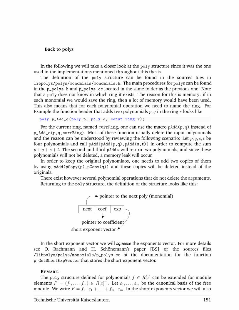
Back to polys
In the following we will take a closer look at the poly structure since it was the oneused in the implementations mentioned throughout this thesis.
The definition of the poly structure can be found in the sources files inlibpolys/polys/monomials/monomials.h. The main procedures for polys can be foundin the p_polys.h and p_polys.cc located in the same folder as the previous one. Notethat a poly does not know in which ring it exists. The reason for this is memory: if ineach monomial we would save the ring, then a lot of memory would have been used.This also means that for each polynomial operation we need to name the ring. ForExample the function header that adds two polynomials p, q in the ring r looks like
poly p_Add_q(poly p, poly q, const ring r);
For the current ring, named currRing, one can use the macro pAdd(p,q) instead ofp_Add_q(p,q,currRing). Most of these function usually delete the input polynomialsand the reason can be understood by reviewing the following scenario: Let p, q, s, t befour polynomials and call pAdd(pAdd(p,q),pAdd(s,t)) in order to compute the sump+ q + s+ t. The second and third pAdd’s will return two polynomials, and since thesepolynomials will not be deleted, a memory leak will occur.
In order to keep the original polynomiaos, one needs to add two copies of themby using pAdd(pCopy(p),pCopy(q)) and these copies will be deleted instead of theoriginals.
There exist however several polynomial operations that do not delete the arguments.Returning to the poly structure, the definition of the structure looks like this:
next coef exp
pointer to the next poly (monomial)
pointer to coefficient
short exponent vector
In the short exponent vector we will squeeze the exponents vector. For more detailssee O. Bachmann and H. Schonemann’s paper [BS] or the sources files/libpolys/polys/monomials/p_polys.cc at the documentation for the functionp_GetShortExpVector that stores the short exponent vector.
REMARK.The poly structure defined for polynomials f ∈ R[x] can be extended for module
elements F = (f1, . . . , fm) ∈ R[x]m. Let ε1, . . . , εm be the canonical basis of the freemodule. We write F = f1 · ε1 + . . .+ fm · εm. In the short exponents vector we will also
Technische Universitat Kaiserslautern 151
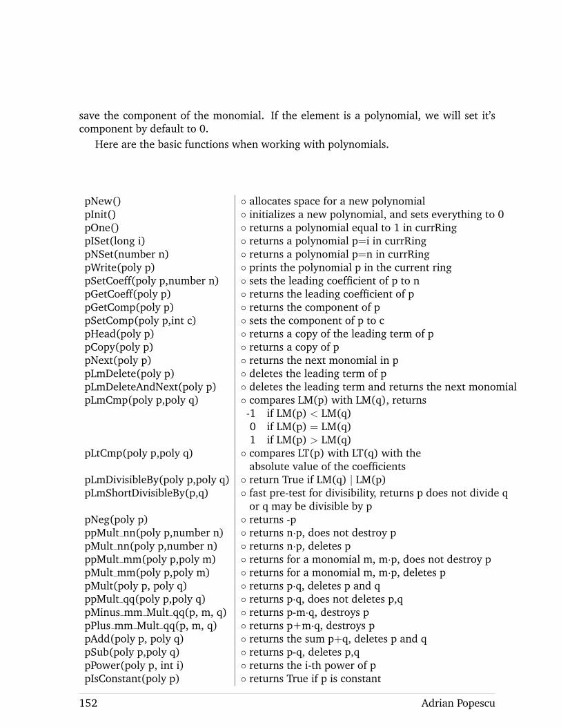
save the component of the monomial. If the element is a polynomial, we will set it’scomponent by default to 0.
Here are the basic functions when working with polynomials.
pNew() ◦ allocates space for a new polynomialpInit() ◦ initializes a new polynomial, and sets everything to 0pOne() ◦ returns a polynomial equal to 1 in currRingpISet(long i) ◦ returns a polynomial p=i in currRingpNSet(number n) ◦ returns a polynomial p=n in currRingpWrite(poly p) ◦ prints the polynomial p in the current ringpSetCoeff(poly p,number n) ◦ sets the leading coefficient of p to npGetCoeff(poly p) ◦ returns the leading coefficient of ppGetComp(poly p) ◦ returns the component of ppSetComp(poly p,int c) ◦ sets the component of p to cpHead(poly p) ◦ returns a copy of the leading term of ppCopy(poly p) ◦ returns a copy of ppNext(poly p) ◦ returns the next monomial in ppLmDelete(poly p) ◦ deletes the leading term of ppLmDeleteAndNext(poly p) ◦ deletes the leading term and returns the next monomialpLmCmp(poly p,poly q) ◦ compares LM(p) with LM(q), returns
-1 if LM(p) < LM(q)0 if LM(p) = LM(q)1 if LM(p) > LM(q)
pLtCmp(poly p,poly q) ◦ compares LT(p) with LT(q) with theabsolute value of the coefficients
pLmDivisibleBy(poly p,poly q) ◦ return True if LM(q) | LM(p)pLmShortDivisibleBy(p,q) ◦ fast pre-test for divisibility, returns p does not divide q
or q may be divisible by ppNeg(poly p) ◦ returns -pppMult nn(poly p,number n) ◦ returns n·p, does not destroy ppMult nn(poly p,number n) ◦ returns n·p, deletes pppMult mm(poly p,poly m) ◦ returns for a monomial m, m·p, does not destroy ppMult mm(poly p,poly m) ◦ returns for a monomial m, m·p, deletes ppMult(poly p, poly q) ◦ returns p·q, deletes p and qppMult qq(poly p,poly q) ◦ returns p·q, does not deletes p,qpMinus mm Mult qq(p, m, q) ◦ returns p-m·q, destroys ppPlus mm Mult qq(p, m, q) ◦ returns p+m·q, destroys ppAdd(poly p, poly q) ◦ returns the sum p+q, deletes p and qpSub(poly p,poly q) ◦ returns p-q, deletes p,qpPower(poly p, int i) ◦ returns the i-th power of ppIsConstant(poly p) ◦ returns True if p is constant
152 Adrian Popescu
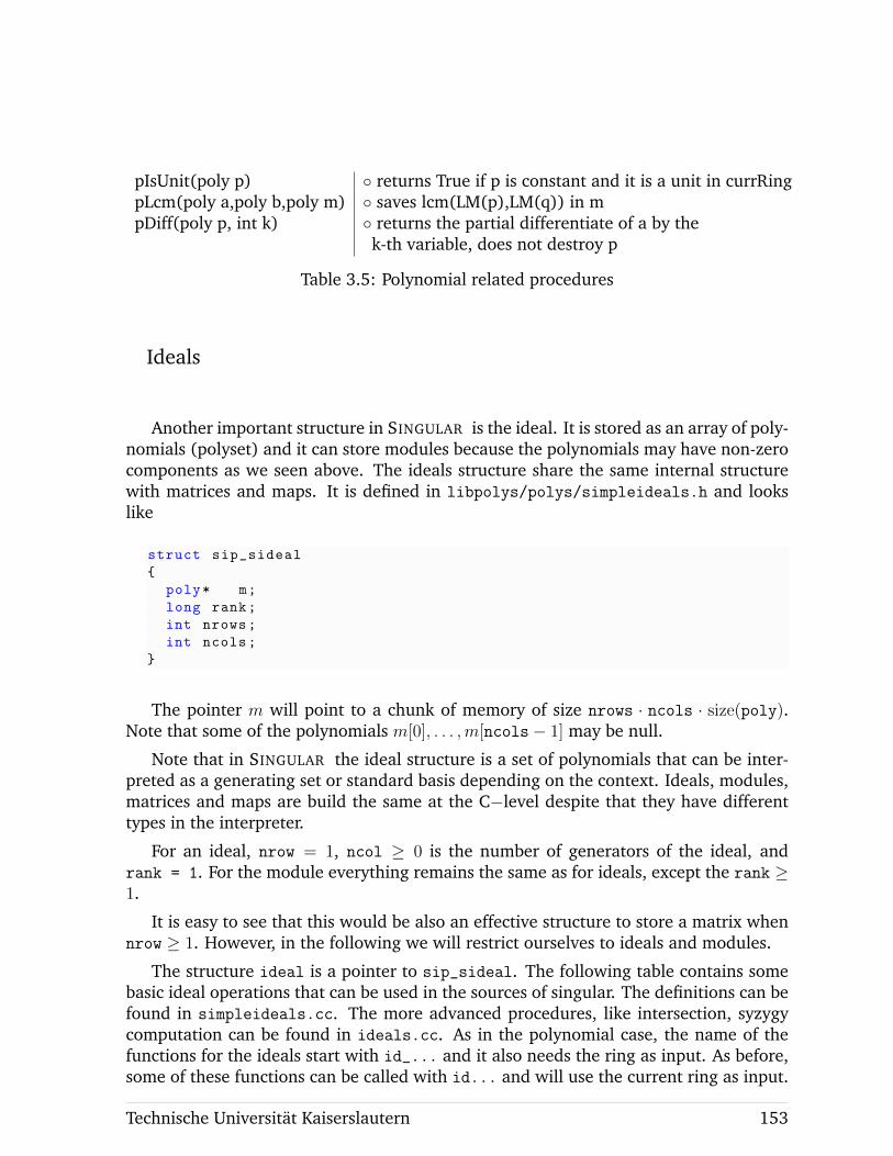
pIsUnit(poly p) ◦ returns True if p is constant and it is a unit in currRingpLcm(poly a,poly b,poly m) ◦ saves lcm(LM(p),LM(q)) in mpDiff(poly p, int k) ◦ returns the partial differentiate of a by the
k-th variable, does not destroy p
Table 3.5: Polynomial related procedures
Ideals
Another important structure in SINGULAR is the ideal. It is stored as an array of poly-nomials (polyset) and it can store modules because the polynomials may have non-zerocomponents as we seen above. The ideals structure share the same internal structurewith matrices and maps. It is defined in libpolys/polys/simpleideals.h and lookslike
struct sip_sideal
{
poly* m;
long rank;
int nrows;
int ncols;
}
The pointer m will point to a chunk of memory of size nrows · ncols · size(poly).Note that some of the polynomials m[0], . . . ,m[ncols− 1] may be null.
Note that in SINGULAR the ideal structure is a set of polynomials that can be inter-preted as a generating set or standard basis depending on the context. Ideals, modules,matrices and maps are build the same at the C−level despite that they have differenttypes in the interpreter.
For an ideal, nrow = 1, ncol ≥ 0 is the number of generators of the ideal, andrank = 1. For the module everything remains the same as for ideals, except the rank ≥1.
It is easy to see that this would be also an effective structure to store a matrix whennrow ≥ 1. However, in the following we will restrict ourselves to ideals and modules.
The structure ideal is a pointer to sip_sideal. The following table contains somebasic ideal operations that can be used in the sources of singular. The definitions can befound in simpleideals.cc. The more advanced procedures, like intersection, syzygycomputation can be found in ideals.cc. As in the polynomial case, the name of thefunctions for the ideals start with id_... and it also needs the ring as input. As before,some of these functions can be called with id... and will use the current ring as input.
Technische Universitat Kaiserslautern 153
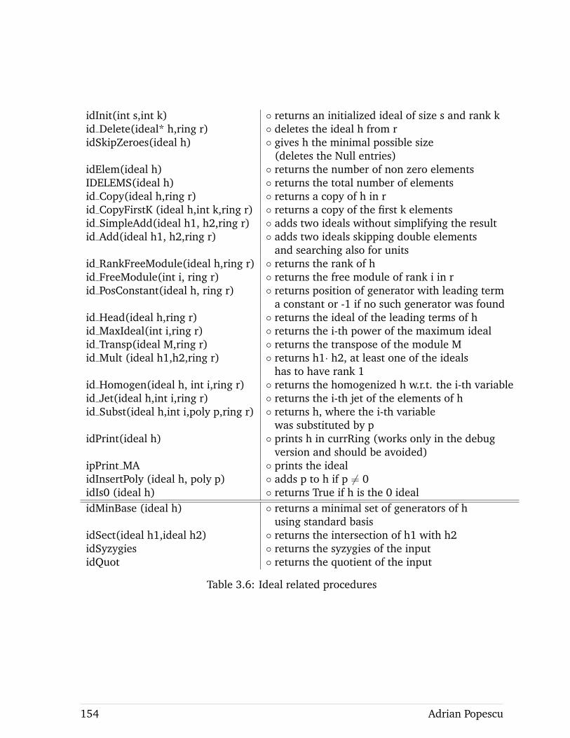
idInit(int s,int k) ◦ returns an initialized ideal of size s and rank kid Delete(ideal* h,ring r) ◦ deletes the ideal h from ridSkipZeroes(ideal h) ◦ gives h the minimal possible size
(deletes the Null entries)idElem(ideal h) ◦ returns the number of non zero elementsIDELEMS(ideal h) ◦ returns the total number of elementsid Copy(ideal h,ring r) ◦ returns a copy of h in rid CopyFirstK (ideal h,int k,ring r) ◦ returns a copy of the first k elementsid SimpleAdd(ideal h1, h2,ring r) ◦ adds two ideals without simplifying the resultid Add(ideal h1, h2,ring r) ◦ adds two ideals skipping double elements
and searching also for unitsid RankFreeModule(ideal h,ring r) ◦ returns the rank of hid FreeModule(int i, ring r) ◦ returns the free module of rank i in rid PosConstant(ideal h, ring r) ◦ returns position of generator with leading term
a constant or -1 if no such generator was foundid Head(ideal h,ring r) ◦ returns the ideal of the leading terms of hid MaxIdeal(int i,ring r) ◦ returns the i-th power of the maximum idealid Transp(ideal M,ring r) ◦ returns the transpose of the module Mid Mult (ideal h1,h2,ring r) ◦ returns h1· h2, at least one of the ideals
has to have rank 1id Homogen(ideal h, int i,ring r) ◦ returns the homogenized h w.r.t. the i-th variableid Jet(ideal h,int i,ring r) ◦ returns the i-th jet of the elements of hid Subst(ideal h,int i,poly p,ring r) ◦ returns h, where the i-th variable
was substituted by pidPrint(ideal h) ◦ prints h in currRing (works only in the debug
version and should be avoided)ipPrint MA ◦ prints the idealidInsertPoly (ideal h, poly p) ◦ adds p to h if p 6= 0idIs0 (ideal h) ◦ returns True if h is the 0 idealidMinBase (ideal h) ◦ returns a minimal set of generators of h
using standard basisidSect(ideal h1,ideal h2) ◦ returns the intersection of h1 with h2idSyzygies ◦ returns the syzygies of the inputidQuot ◦ returns the quotient of the input
Table 3.6: Ideal related procedures
154 Adrian Popescu
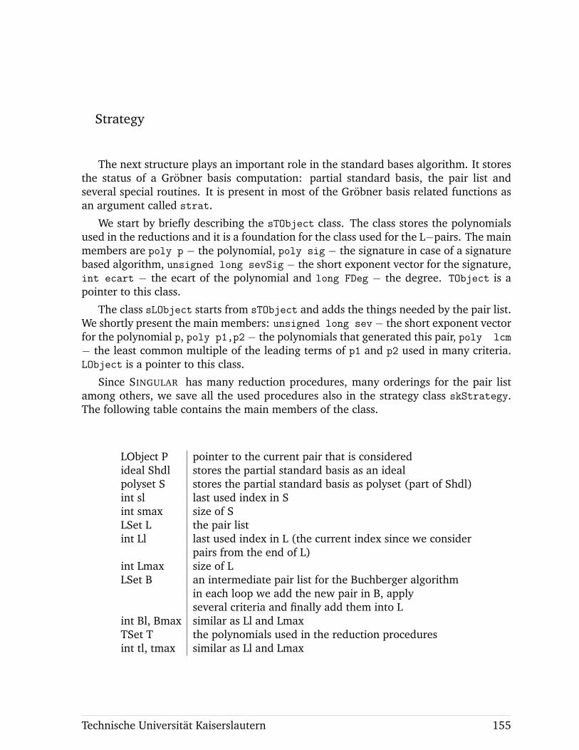
Strategy
The next structure plays an important role in the standard bases algorithm. It storesthe status of a Grobner basis computation: partial standard basis, the pair list andseveral special routines. It is present in most of the Grobner basis related functions asan argument called strat.
We start by briefly describing the sTObject class. The class stores the polynomialsused in the reductions and it is a foundation for the class used for the L−pairs. The mainmembers are poly p − the polynomial, poly sig − the signature in case of a signaturebased algorithm, unsigned long sevSig − the short exponent vector for the signature,int ecart − the ecart of the polynomial and long FDeg − the degree. TObject is apointer to this class.
The class sLObject starts from sTObject and adds the things needed by the pair list.We shortly present the main members: unsigned long sev− the short exponent vectorfor the polynomial p, poly p1,p2 − the polynomials that generated this pair, poly lcm
− the least common multiple of the leading terms of p1 and p2 used in many criteria.LObject is a pointer to this class.
Since SINGULAR has many reduction procedures, many orderings for the pair listamong others, we save all the used procedures also in the strategy class skStrategy.The following table contains the main members of the class.
LObject P pointer to the current pair that is consideredideal Shdl stores the partial standard basis as an idealpolyset S stores the partial standard basis as polyset (part of Shdl)int sl last used index in Sint smax size of SLSet L the pair listint Ll last used index in L (the current index since we consider
pairs from the end of L)int Lmax size of LLSet B an intermediate pair list for the Buchberger algorithm
in each loop we add the new pair in B, applyseveral criteria and finally add them into L
int Bl, Bmax similar as Ll and LmaxTSet T the polynomials used in the reduction proceduresint tl, tmax similar as Ll and Lmax
Technische Universitat Kaiserslautern 155
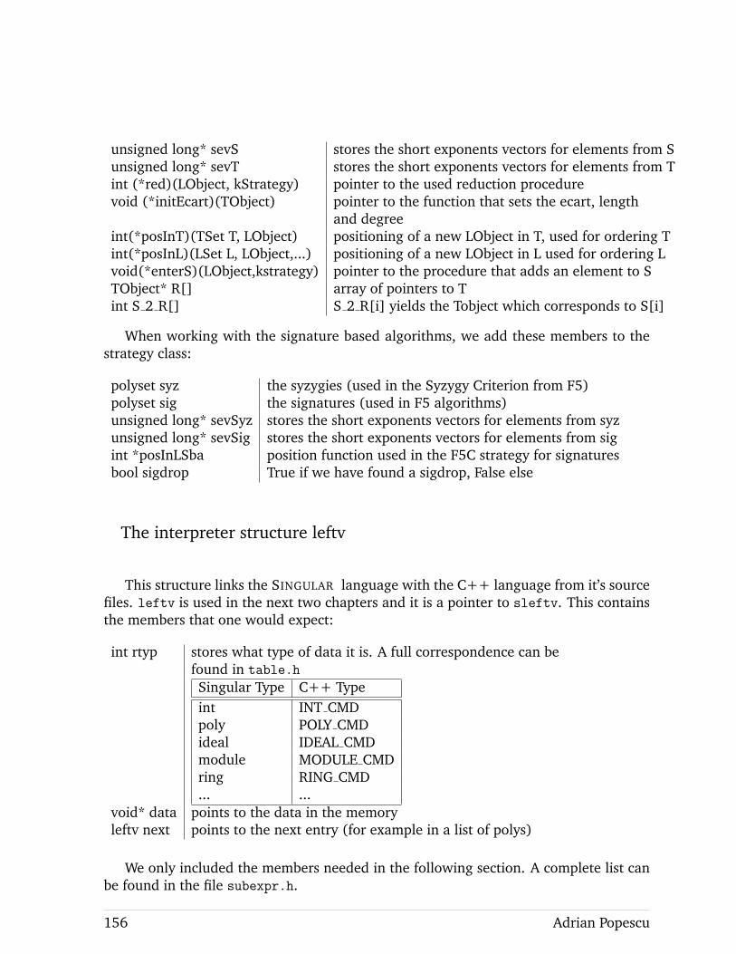
unsigned long* sevS stores the short exponents vectors for elements from Sunsigned long* sevT stores the short exponents vectors for elements from Tint (*red)(LObject, kStrategy) pointer to the used reduction procedurevoid (*initEcart)(TObject) pointer to the function that sets the ecart, length
and degreeint(*posInT)(TSet T, LObject) positioning of a new LObject in T, used for ordering Tint(*posInL)(LSet L, LObject,...) positioning of a new LObject in L used for ordering Lvoid(*enterS)(LObject,kstrategy) pointer to the procedure that adds an element to STObject* R[] array of pointers to Tint S 2 R[] S 2 R[i] yields the Tobject which corresponds to S[i]
When working with the signature based algorithms, we add these members to thestrategy class:
polyset syz the syzygies (used in the Syzygy Criterion from F5)polyset sig the signatures (used in F5 algorithms)unsigned long* sevSyz stores the short exponents vectors for elements from syzunsigned long* sevSig stores the short exponents vectors for elements from sigint *posInLSba position function used in the F5C strategy for signaturesbool sigdrop True if we have found a sigdrop, False else
The interpreter structure leftv
This structure links the SINGULAR language with the C++ language from it’s sourcefiles. leftv is used in the next two chapters and it is a pointer to sleftv. This containsthe members that one would expect:
int rtyp stores what type of data it is. A full correspondence can befound in table.h
Singular Type C++ Typeint INT CMDpoly POLY CMDideal IDEAL CMDmodule MODULE CMDring RING CMD... ...
void* data points to the data in the memoryleftv next points to the next entry (for example in a list of polys)
We only included the members needed in the following section. A complete list canbe found in the file subexpr.h.
156 Adrian Popescu
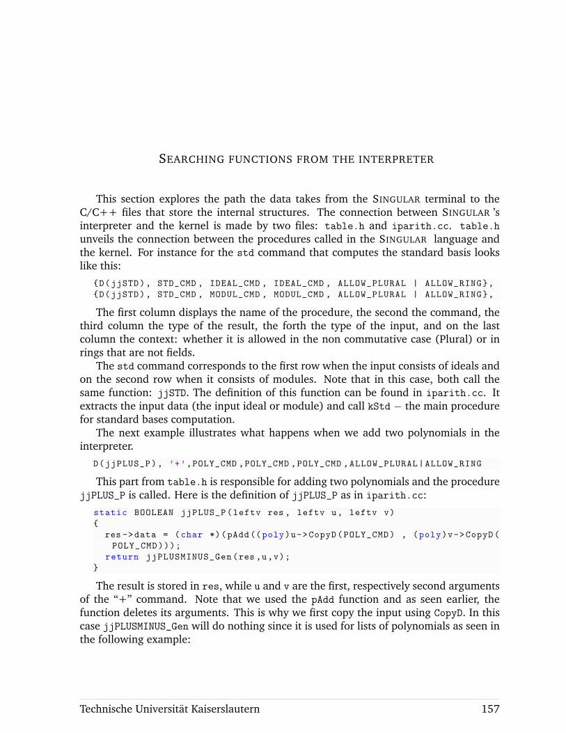
SEARCHING FUNCTIONS FROM THE INTERPRETER
This section explores the path the data takes from the SINGULAR terminal to theC/C++ files that store the internal structures. The connection between SINGULAR ’sinterpreter and the kernel is made by two files: table.h and iparith.cc. table.h
unveils the connection between the procedures called in the SINGULAR language andthe kernel. For instance for the std command that computes the standard basis lookslike this:
{D(jjSTD), STD_CMD , IDEAL_CMD , IDEAL_CMD , ALLOW_PLURAL | ALLOW_RING},
{D(jjSTD), STD_CMD , MODUL_CMD , MODUL_CMD , ALLOW_PLURAL | ALLOW_RING},
The first column displays the name of the procedure, the second the command, thethird column the type of the result, the forth the type of the input, and on the lastcolumn the context: whether it is allowed in the non commutative case (Plural) or inrings that are not fields.
The std command corresponds to the first row when the input consists of ideals andon the second row when it consists of modules. Note that in this case, both call thesame function: jjSTD. The definition of this function can be found in iparith.cc. Itextracts the input data (the input ideal or module) and call kStd − the main procedurefor standard bases computation.
The next example illustrates what happens when we add two polynomials in theinterpreter.
D(jjPLUS_P), ’+’,POLY_CMD ,POLY_CMD ,POLY_CMD ,ALLOW_PLURAL|ALLOW_RING
This part from table.h is responsible for adding two polynomials and the procedurejjPLUS_P is called. Here is the definition of jjPLUS_P as in iparith.cc:
static BOOLEAN jjPLUS_P(leftv res , leftv u, leftv v)
{
res ->data = (char *)(pAdd((poly)u->CopyD(POLY_CMD) , (poly)v->CopyD(
POLY_CMD)));
return jjPLUSMINUS_Gen(res ,u,v);
}
The result is stored in res, while u and v are the first, respectively second argumentsof the “+” command. Note that we used the pAdd function and as seen earlier, thefunction deletes its arguments. This is why we first copy the input using CopyD. In thiscase jjPLUSMINUS_Gen will do nothing since it is used for lists of polynomials as seen inthe following example:
Technische Universitat Kaiserslautern 157
ring r = 0,(x,y),dp;
list p = x,y;
list q = x2 ,y;
p[1..2]+q[1..2];
//>x+x2 2y
An example worth analyzing in depth is the standard basis algorithm. The partresponsible for the standard bases algorithms is located in the folder kernel/GBEngine.The main files are:
kstd1.cc handles the local and mixed case of the standard basis andcontains also several reduction procedures
kstd2.cc handles the global case of standard basis andcontains several reduction procedures
kutil.h defines the class for TObjects and LObjectskutil.cc contains many functions including different positioning, adding new
pairs and initializing parts of the used strategykspoly.cc defines functions needed for the computation of a new s−polynomial
or reduction stepskInline.h defines TObjects and LObjects related functions
Earlier we saw that when the command std is called in SINGULAR , we linked it tojjSTD defined in the file iparith.cc. Here, after extracting the input from the leftv
structure, we run the function kStd. This is the main standard basis function and itis defined in kstd1.cc. kStd takes as input the ideals F and Q, where F is the inputideal and Q is the quotient ideal in the case of a quotient ring (qring), the weights incase of a weighted ordering and several flags. In kStd a new strategy is defined, wherewe set some flags like the homogeneity of the input and check for example whether theordering is a lexicographic ordering or not. If the monomial ordering is a global one, bba(Buchberger algorithm) defined in kstd2.cc is called. Otherwise mora (Mora algorithm− the generalization of Buchberger for local cases considering the ecart) defined inkstd1.cc.
The next step in both functions is setting the strategy. This is denoted by the objectstrat of kStrategy type as seen in the earlier section.
initBuchMoraPos sets the positioning functions for the set T and LinitBuchMoraCrit sets the used criteriainitBba / initMora sets the reduction procedures, enterS and initEcartinitBuchMora initializes the sets S, L and T and
adds the input as initial pairs to L
Then, as in Buchbergers algorithm, we loop till the set L is empty and take the lastelement from the pair list (since it is the smallest element with respect to the chosenpair ordering). P will point to this pair. Usually we compute for the pairs the so-called
158 Adrian Popescu
short s−polynomial, namely the leading term of the normal s−polynomial, used sinceit consumes less memory. If P is a short s−polynomial, we need to build the normal oneand we start by reducing and tail reducing it with the set T.
If it can be reduced to 0, then simply delete this pair and continue with the next loop.However, if we obtained a non zero polynomial, we have to add the s−polynomials tothe pair list L when working over fields (enterpairs) or add the corresponding strongpolynomials, s−pairs and the extended polynomial (superenterpairs) to L when com-puting over rings. Next, add the element to the reduction set T and to the partialstandard basis S. In the case of fields, we first add the new pairs to the set B and afterapplying several criteria on the set B, we add it to L.
At the end we do a complete reduction and delete the sets L,T and at the end of kStdwe delete the strategy.
Technische Universitat Kaiserslautern 159

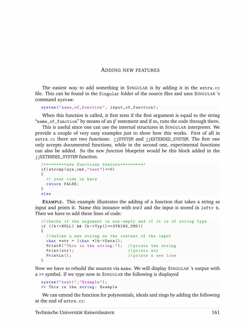
ADDING NEW FEATURES
The easiest way to add something in SINGULAR is by adding it in the extra.cc
file. This can be found in the Singular folder of the source files and uses SINGULAR ’scommand system:
system("name_of_function", input_of_function);
When this function is called, it first tests if the first argument is equal to the string“name_of_function” by means of an if statement and if so, runs the code through there.
This is useful since one can use the internal structures in SINGULAR interpreter. Weprovide a couple of very easy examples just to show how this works. First of all inextra.cc there are two functions: jjSYSTEM and jjEXTENDED_SYSTEM. The first oneonly accepts documented functions, while in the second one, experimental functionscan also be added. So the new function blueprint would be this block added in thejjEXTENDED_SYSTEM function.
/* ======== new functions feature ======== */
if(strcmp(sys_cmd ,"test")==0)
{
// your code in here
return FALSE;
}
else
EXAMPLE. This example illustrates the adding of a function that takes a string asinput and prints it. Name this instance with test1 and the input is stored in leftv h.Then we have to add these lines of code:
// checks if the argument is non -empty and if it is of string type
if ((h!=NULL) && (h->Typ()== STRING_CMD))
{
// define a new string as the content of the input
char *str = (char *)h->Data();
PrintS("This is the string:"); // prints the string
Print(str); // prints str
PrintLn (); // prints a new line
}
Now we have to rebuild the sources via make. We will display SINGULAR ’s output witha >> symbol. If we type now in SINGULAR the following is displayed
system("test1","Example");
>> This is the string: Example
We can extend the function for polynomials, ideals and rings by adding the followingat the end of extra.cc:
Technische Universitat Kaiserslautern 161
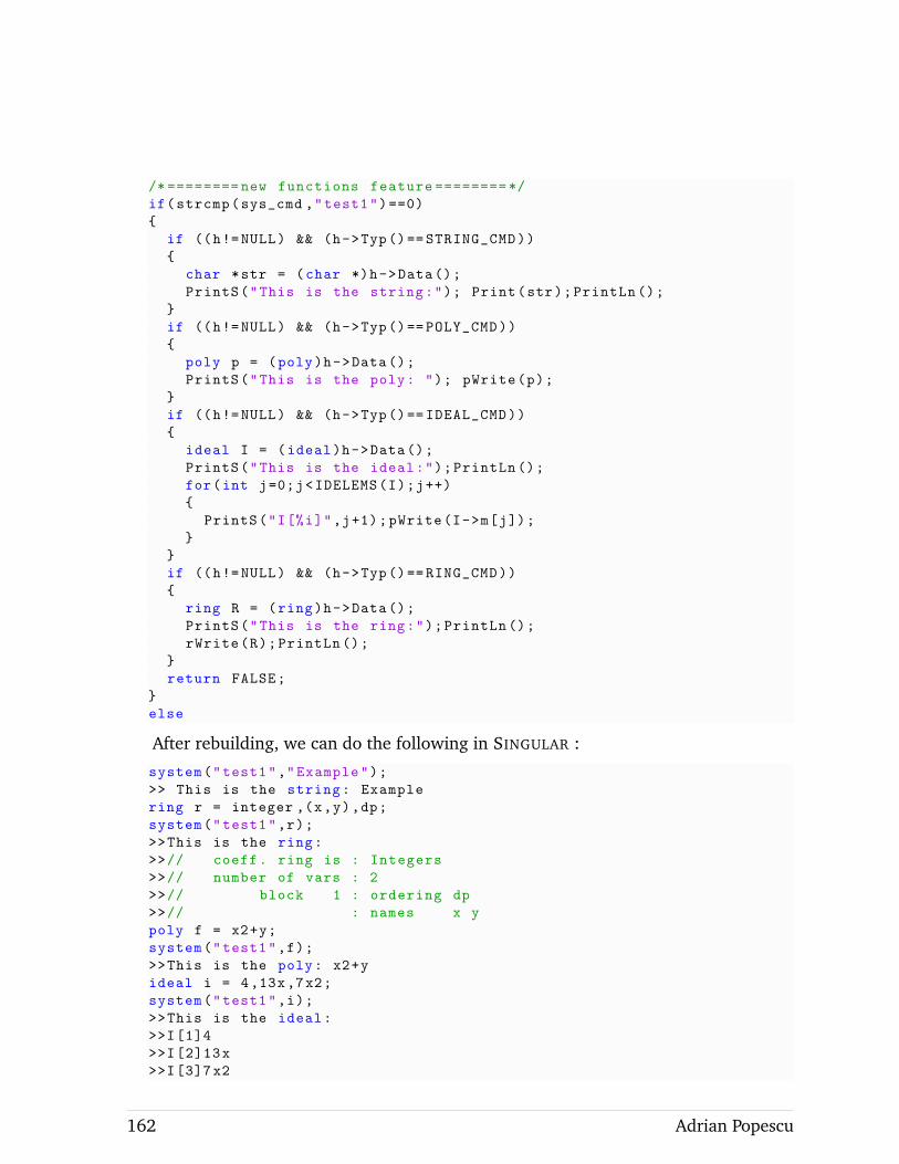
/* ======== new functions feature ======== */
if(strcmp(sys_cmd ,"test1")==0)
{
if ((h!=NULL) && (h->Typ()== STRING_CMD))
{
char *str = (char *)h->Data();
PrintS("This is the string:"); Print(str);PrintLn ();
}
if ((h!=NULL) && (h->Typ()== POLY_CMD))
{
poly p = (poly)h->Data();
PrintS("This is the poly: "); pWrite(p);
}
if ((h!=NULL) && (h->Typ()== IDEAL_CMD))
{
ideal I = (ideal)h->Data();
PrintS("This is the ideal:");PrintLn ();
for(int j=0;j<IDELEMS(I);j++)
{
PrintS("I[%i]",j+1);pWrite(I->m[j]);
}
}
if ((h!=NULL) && (h->Typ()== RING_CMD))
{
ring R = (ring)h->Data();
PrintS("This is the ring:");PrintLn ();
rWrite(R);PrintLn ();
}
return FALSE;
}
else
After rebuilding, we can do the following in SINGULAR :
system("test1","Example");
>> This is the string: Example
ring r = integer ,(x,y),dp;
system("test1",r);
>>This is the ring:
>>// coeff. ring is : Integers
>>// number of vars : 2
>>// block 1 : ordering dp
>>// : names x y
poly f = x2+y;
system("test1",f);
>>This is the poly: x2+y
ideal i = 4,13x,7x2;
system("test1",i);
>>This is the ideal:
>>I[1]4
>>I[2]13x
>>I[3]7x2
162 Adrian Popescu
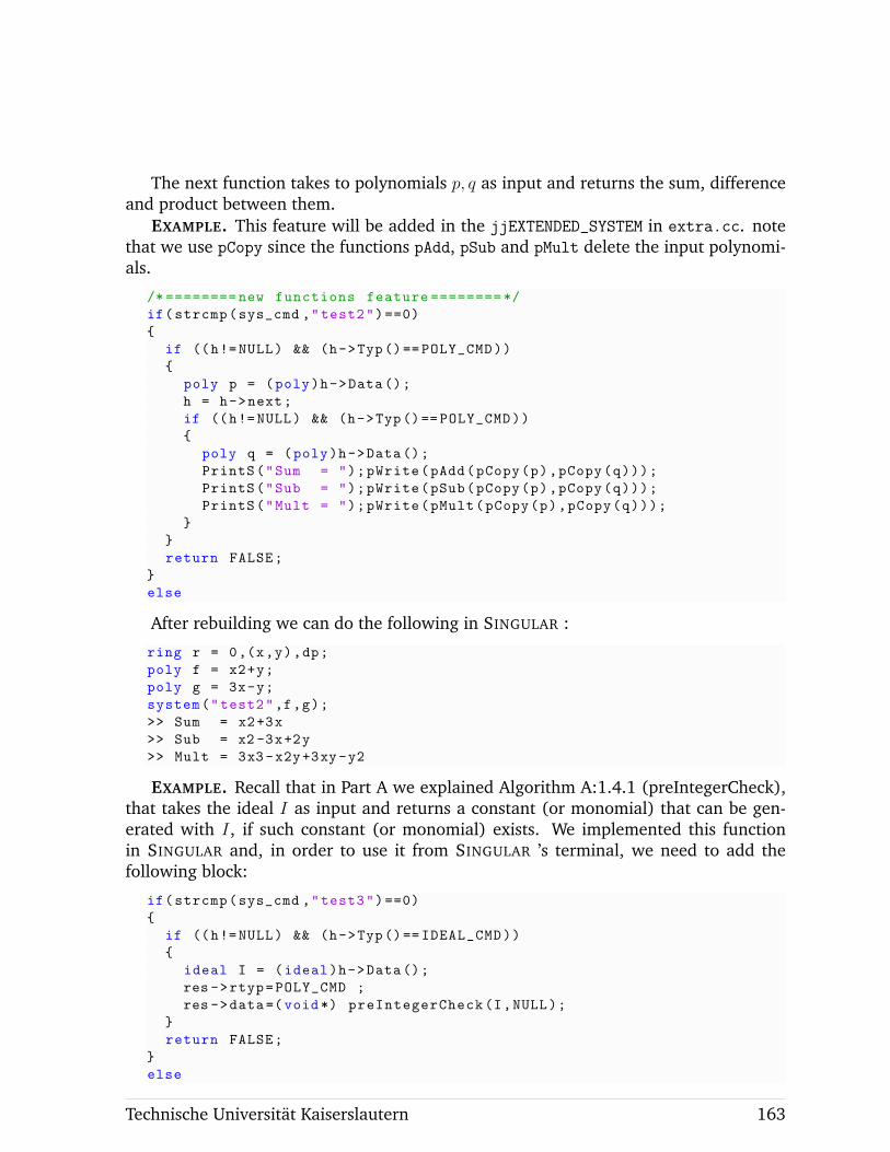
The next function takes to polynomials p, q as input and returns the sum, differenceand product between them.
EXAMPLE. This feature will be added in the jjEXTENDED_SYSTEM in extra.cc. notethat we use pCopy since the functions pAdd, pSub and pMult delete the input polynomi-als.
/* ======== new functions feature ======== */
if(strcmp(sys_cmd ,"test2")==0)
{
if ((h!=NULL) && (h->Typ()== POLY_CMD))
{
poly p = (poly)h->Data();
h = h->next;
if ((h!=NULL) && (h->Typ()== POLY_CMD))
{
poly q = (poly)h->Data();
PrintS("Sum = ");pWrite(pAdd(pCopy(p),pCopy(q)));
PrintS("Sub = ");pWrite(pSub(pCopy(p),pCopy(q)));
PrintS("Mult = ");pWrite(pMult(pCopy(p),pCopy(q)));
}
}
return FALSE;
}
else
After rebuilding we can do the following in SINGULAR :
ring r = 0,(x,y),dp;
poly f = x2+y;
poly g = 3x-y;
system("test2",f,g);
>> Sum = x2+3x
>> Sub = x2 -3x+2y
>> Mult = 3x3 -x2y+3xy -y2
EXAMPLE. Recall that in Part A we explained Algorithm A:1.4.1 (preIntegerCheck),that takes the ideal I as input and returns a constant (or monomial) that can be gen-erated with I, if such constant (or monomial) exists. We implemented this functionin SINGULAR and, in order to use it from SINGULAR ’s terminal, we need to add thefollowing block:
if(strcmp(sys_cmd ,"test3")==0)
{
if ((h!=NULL) && (h->Typ()== IDEAL_CMD))
{
ideal I = (ideal)h->Data();
res ->rtyp=POLY_CMD ;
res ->data=(void*) preIntegerCheck(I,NULL);
}
return FALSE;
}
else
Technische Universitat Kaiserslautern 163
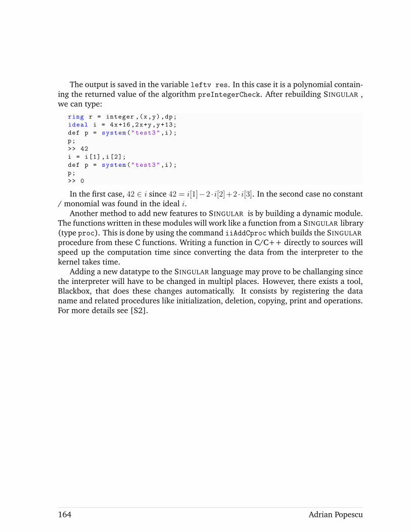
The output is saved in the variable leftv res. In this case it is a polynomial contain-ing the returned value of the algorithm preIntegerCheck. After rebuilding SINGULAR ,we can type:
ring r = integer ,(x,y),dp;
ideal i = 4x+16,2x+y,y+13;
def p = system("test3",i);
p;
>> 42
i = i[1],i[2];
def p = system("test3",i);
p;
>> 0
In the first case, 42 ∈ i since 42 = i[1]−2 · i[2]+2 · i[3]. In the second case no constant/ monomial was found in the ideal i.
Another method to add new features to SINGULAR is by building a dynamic module.The functions written in these modules will work like a function from a SINGULAR library(type proc). This is done by using the command iiAddCproc which builds the SINGULAR
procedure from these C functions. Writing a function in C/C++ directly to sources willspeed up the computation time since converting the data from the interpreter to thekernel takes time.
Adding a new datatype to the SINGULAR language may prove to be challanging sincethe interpreter will have to be changed in multipl places. However, there exists a tool,Blackbox, that does these changes automatically. It consists by registering the dataname and related procedures like initialization, deletion, copying, print and operations.For more details see [S2].
164 Adrian Popescu

Technische Universitat Kaiserslautern 165

REFERENCES
[CoCoA] J. Abbott, A. M. Bigatti, CoCoALib: a C++ library for doing Computationsin Commutative Algebra, available at http://cocoa.dima.unige.it/cocoalib.
[Artin1] M. Artin, Algebraic approximation of structures over complete local rings,Publ. Math. IHES, 36, (1969), 23-58.
[Artin2] M. Artin, Constructions technques for algebraic spaces, Actes Congres. Intern.Math., (1970), 419-423.
[BS] O. Bachmann and H. Schonemann, Monomial representations for Grobnerbases computations, ISSAC ’98, (1998), 309-316.
[BGS] A.M. Bigatti, P. Gimenez, E. Saenz-de-Cabezon, Monomial Ideals, Computa-tions and Applications, Springer, (2013).
[BiHo] C. Biro, D.M. Howard, M.T. Keller, W.T. Trotter, S.J. Young, Interval parti-tions and Stanley depth, J. Combin. Theory, Ser. A, 117, (2010), 475-482.
[BH] W. Bruns, J. Herzog, Cohen-Macaulay rings, Revised edition. CambridgeUniversity Press, (1998).
[BIS] W. Bruns, B. Ichim, C. Soger, The power of pyramid decomposition in Nor-maliz, J. Symb. Comp., 54, (2016), 513-536.
[BKU] W. Bruns, C. Krattenthaler, J. Uliczka, Stanley decompositions and Hilbertdepth in the Koszul complex, J. Commutative Alg., 2, (2010), 327-357.
[BMU] W. Bruns, J. Moyano-Fernandez, J. Uliczka, Hilbert regularity of ZZ-gradedmodules over polynomial rings, (2013), arXiv:AC/1308.2917.
[Bu] B. Buchberger, Ein Algorithmus zum Auffinden der Basiselemente des Restk-lassenringes nach einem nulldimensionalen Polynomideal, PhD thesis, Uni-versity of Innsbruck, (1965).
[Ci] M. Cimpoeas, Stanley depth of complete intersection monomial ideals, Bull.Math. Soc. Sc. Math. Roumanie 51(99), (2008), 205-211.
[Singular] W. Decker, G.-M. Greuel, G. Pfister, H. Schonemann, SINGULAR 4-1-3— A computer algebra system for polynomial computations, available atwww.singular.uni-kl.de, (2016).
Technische Universitat Kaiserslautern 167
[DuGo] A. Duval, B. Goeckner, C. Klivans, J. Martin, A non-partitionable Cohen-Macaulay simplicial complex, Adv. Math., 299, (2016), 381-395.
[E] C. Eder, Signature-based algorithms to compute standard bases, PhD thesis,University of Kaiserslautern, (2012).
[EF] C. Eder, J.-C. Faugere, A survey on signature-based Grobner basis computa-tions, arXiv:AC/1404.1774, (2014).
[EP] C. Eder, J. Perry, F5C: A variant of Faugeres F5 algorithm with reducedGrobner bases, J. of Symb. Comp., 45, 12, (2010), 1442-1458.
[EPP] C. Eder, G. Pfister, A. Popescu New Strategies for Standard Bases over Z,(2016), arXiv:AC/1609.04257.
[El] R. Elkik, Solutions d’equations a coefficients dans un anneaux henselien, Ann.Sci. Ecole Normale Sup., 6, (1973), 553-604.
[F] J.-C. Faugere, A new efficient algorithm for computing Grobner bases withoutreduction to zero F5, ISSAC 2002, (2002), 75-82.
[G] H. Grauert, Uber die Deformation isolierter Singularitaten analytischer Men-gen, Inventiones Mathematicae, 15, (1972), 171-198.
[Gr] M. Greenberg, Rational points in henselian discrete valuation rings, Publ.Math. IHES, 31, (1966), 59-64.
[GP] G.-M. Greuel, G. Pfister, A SINGULAR Introduction to Commutative Algebra,Springer-Verlag, (2008).
[GD] A. Grothedieck, J. Dieudonne, Elements de geometrie algebrique, IV, Part 1,Publ. Math. IHES, (1966).
[H] J. Herzog, A Survey on Stanley Depth, Lecture Notes in Mathematics,Springer-Verlag, (2013).
[HPV] J. Herzog, D. Popescu, M. Vladoiu, Stanley depth and size of a monomialideal, Proc. Amer. Math. Soc., 140, (2012), 493-504.
[HSY] J. Herzog, A. Soleyman Jahann, S. Yassemi, Stanley decompositions andpartitionable simplicial complexes, J. Alg. Comb., 27, (2008), 113-125.
[HVZ] J. Herzog, M. Vladoiu, X. Zheng, How to compute the Stanley depth of amonomial ideal, J. Algebra, 322, (2009), 3151-3169.
[Hi] H. Hironaka, Resolution of Singularities of an Algebraic Variety over a Fieldof Characteristic Zero, Annals of Mathematics, 79, (1964).
168 Adrian Popescu
[IKM] B. Ichim, L. Katthan, J. J. Moyano-Fernandez, The behaviour of Stanleydepth under polarization, J. Comb. Theory, Series A, 135, (2015), 332-347.
[IM] B. Ichim, J. J. Moyano-Fernandez, How to compute the multigraded Hilbertdepth of a module, Math. Nachr. 287, No. 11-12, (2014), 1274-1287,arXiv:AC/1209.0084v3.
[IZ] B. Ichim, A. Zarojanu, An algorithm for computing the multigraded Hilbertdepth of a module, Experimental Mathematics, 23:3, (2014), 322-331,arXiv:AC/1304.7215v3.
[Is] M. Ishaq, Upper bounds for the Stanley depth, Comm. in Alg., 40, (2012),87-97.
[IsQu] M. Ishaq, M. I. Qureshi, Upper and lower bounds for the Stanley depth ofcertain classes of monomial ideals and their residue class rings, Comm. inAlg., Volume 41, (2013), 1107-1116.
[Ka] L. Katthan, Stanley depth and simplicial spanning trees, J. of Algebraic Com-binatorics, 42, (2015), 507-536.
[KMPPR] H. Kurke, T. Mostowski, G. Pfister, D. Popescu, M. Roczen, Die Approxima-tionseigenschaft lokaler Ringe, Springer Lect. Notes in Math., 634, Springer-Verlag, Berlin-New York, (1978).
[Li] D. Lichtblau, Effective computation of strong Grobner bases over Euclideandomains, Illinois J. of Math. 56(1), (2012), 177-194.
[Ly] G. Lyubeznik, On the Arithmetical Rank of Monomial ideals, J. of Algebra112, (1988), 86-89.
[MS] J. Murdock, J. Sanders, A new transvectant algorithm for nilpotent normalforms, J. of Diff. Eq., 238(1), (2007), 234-256.
[Ne] A. Neron, Modeles minimaux des varietes abeliennes sur les corps locaux etglobaux, Publ. Math. IHES, 21, (1964).
[OY] R. Okazaki, K. Yanagawa, Alexander duality and Stanley depth of multi-graded modules, J. of Algebra 340, (2011), 35-52.
[PfPo1] G. Pfister, D. Popescu, Die strenge Approximationseigenschaft lokaler Ringe,Inventiones Math., 30, (1975),145-174.
[PfPo2] G. Pfister, D. Popescu, Constructive General Neron Desingularizationfor one dimensional local rings, to appear in J. of Symb. Comp.,arXiv:AC/1512.08435.
Technische Universitat Kaiserslautern 169
[AP1] A. Popescu, Special Stanley Decompositions, Bull. Math. Soc. Sc. Math.Roumanie, 53(101), (2010), 363-372, arXiv:AC/1008.2924v2.
[AP2] A. Popescu, An algorithm to compute the Hilbert depth , J. of Symb. Comput.,66, (2015), 1-7, arXiv:AC/1307.6084v3.
[AP3] A. Popescu, Depth and Stanley depth of the canonical form of a factor ofmonomial ideals, Bull. Math. Soc. Sc. Math. Roumanie, 57(105), (2014),207-216, arXiv:AC/1402.5826v3
[APDP1] A. Popescu, D. Popescu, Four generated, squarefree, monomial ideals ,in “Bridging Algebra, Geometry, and Topology”, Editors Denis Ibadula,Willem Veys, Springer Proceed. in Math., and Statistics, 96, (2014), 231-248, arXiv:AC/1309.4986v5.
[APDP2] A. Popescu, D. Popescu, A method to compute the General Neron Desingular-ization in the frame of one dimensional local domains, to appear in Singular-ities and Computer Algebra - Festschrift for Gert-Martin Greuel, On the occa-sion of his 70th birthday, Editors W. Decker, G. Pfister, M. Schulze, SpringerMonograph.
[DP1] D. Popescu, General Neron Desingularization, Nagoya Math. J., 100, (1985),97-126.
[DP2] D. Popescu, General Neron Desingularization and approximation, NagoyaMath. J., 104, (1986), 85-115.
[DP3] D. Popescu, Letter to the Editor. General Neron Desingularization and approx-imation, Nagoya Math. J., 118, (1990), 45-53.
[DP4] D. Popescu, Artin Approximation, in “Handbook of Algebra”, vol. 2, Ed. M.Hazewinkel, Elsevier, (2000), 321-355.
[DP5] D. Popescu, Depth of factors of square free monomial ideals, Proceedings ofAMS 142, (2014), 1965-1972, arXiv:AC/1110.1963v5.
[DP6] D. Popescu, Upper bounds of depth of monomial ideals, J. Commutative Al-gebra, 5, (2013), 323-327, arXiv:AC/1206.3977.
[DP7] D. Popescu, Stanley conjecture on intersections of four monomial prime ideals,Comm. in Alg. 41, (2010), 4351-4362.
[DP8] D. Popescu, Around General Neron Desingularization, J. of Alg. and its Appl.,16,(2017).
[PQ] D. Popescu, I. Qureshi, Computing the Stanley depth, J. Algebra, 323,(2010), 2943-2959.
170 Adrian Popescu
[PZ] D. Popescu, A. Zarojanu, Three generated, squarefree, monomial ideals,Bull. Math. Soc. Sci. Math. Roumanie, 58(106), (2015), no 3, 359-368,arXiv:AC/1307.8292v6.
[Ra] A. Rauf, Depth and Stanley depth of multigraded modules, Comm. Algebra,38, (2010), 773-784.
[RTU] G. Restuccia, Z. Tang, R. Utano, Stanley Conjecture on monomial ideals ofmixed products, J. Comm. Alg., 7, (2015), 77-85.
[Ri] G. Rinaldo, An algorithm to compute the Stanley depth of monomial ideals,Le Matematiche, Vol. LXIII, (2008), 243-256.
[Ro] G. Rond, Sur la linearite de la fonction de Artin, Ann. Sci. Ecole Norm. Sup.,(4), 38, (2005), 979-988.
[S1] H. Schonemann, Polynomials in Factory and Singular, Nikolaus-KonferenzAachen, (1999).
[S2] H. Schonemann, Extending Singular with new types and algorithms, Inter-national Congress on Mathematical Software (ICMS), (2016).
[Sh] Y.H. Shen, Lexsegment ideals of Hilbert depth 1, (2012), available atarXiv:AC/1208.1822v1.
[St] R. P. Stanley, Linear Diophantine equations and local cohomology, Invent.Math., 68, (1982), 175-193.
[SW] B. Sturmfels, N. White, Stanley decompositions of the bracket ring, Math.Scand., 67, (1990), 183-189.
[Sw] R. Swan, Neron-Popescu desingularization, in “Algebra and Geometry”, Ed.M. Kang, International Press, Cambridge, (1998), 135-192.
[Ta] Z. Tang, Stanley depth of certain Stanley-Reisner rings, J. Algebra, 409,(2014), 430-443.
[Uli] J. Uliczka, Remarks on Hilbert series of graded modules over polynomial rings,Manuscripta Math., 132 (2010), 159-168.
[Vi] R. H. Villarreal, Monomial Algebras, Marcel Dekker Inc., New York, (2001).
[W] O. Wienand, Algorithms for Symbolic Computation and their Applications -Standard Bases over Rings and Rank Tests in Statistics, PhD thesis, Universityof Kaiserslautern, (2011).
[Y] K. Yanagawa, Sliding functor and polarization functor for multigraded mod-ules, Cummunications in Algebra, 40, (2012), 1151-1166.
Technische Universitat Kaiserslautern 171

WISSENSCHAFTLICHER WERDEGANG
2008 Abitur, Colegiul National Sfantul Sava, Bukarest, Rumanien
2008 - 2011 Bachelor im Mathematik, Universitat Bukarest, Rumanien
2008 - 2011 Level 1: Zertifikat fur Lehramt, Universitat Bukarest, Rumanien
2011 - 2013 Master im Mathematik, Technische Universitat Kaiserslautern
2013 - 2016 Promotion im Mathematik , Technische Universitat Kaiserslautern
CURRICULUM VITAE
2008 Abitur, Colegiul National Sfantul Sava, Bucharest, Romania
2008 - 2011 Bachelor in Mathematics, University of Bucharest, Romania
2008 - 2011 Certification for teaching (I), University of Bucharest, Romania
2011 - 2013 Master in Mathematics, University of Kaiserslautern, Germany
2013 - 2016 PhD in Mathematics , University of Kaiserslautern, Germany
Technische Universitat Kaiserslautern 173

174 Adrian Popescu

Technische Universitat Kaiserslautern 175