econstor www.econstor.eu

Der Open-Access-Publikationsserver der ZBW – Leibniz-Informationszentrum WirtschaftThe Open Access Publication Server of the ZBW – Leibniz Information Centre for Economics

Standard-Nutzungsbedingungen:

Die Dokumente auf EconStor dürfen zu eigenen wissenschaftlichenZwecken und zum Privatgebrauch gespeichert und kopiert werden.

Sie dürfen die Dokumente nicht für öffentliche oder kommerzielleZwecke vervielfältigen, öffentlich ausstellen, öffentlich zugänglichmachen, vertreiben oder anderweitig nutzen.

Sofern die Verfasser die Dokumente unter Open-Content-Lizenzen(insbesondere CC-Lizenzen) zur Verfügung gestellt haben sollten,gelten abweichend von diesen Nutzungsbedingungen die in der dortgenannten Lizenz gewährten Nutzungsrechte.

Terms of use:

Documents in EconStor may be saved and copied for yourpersonal and scholarly purposes.

You are not to copy documents for public or commercialpurposes, to exhibit the documents publicly, to make thempublicly available on the internet, or to distribute or otherwiseuse the documents in public.

If the documents have been made available under an OpenContent Licence (especially Creative Commons Licences), youmay exercise further usage rights as specified in the indicatedlicence.

zbw Leibniz-Informationszentrum WirtschaftLeibniz Information Centre for Economics

Moreno-Cruz, Juan; Taylor, M. Scott

Working Paper

A Spatial Approach to Energy Economics: Theory,Measurement and Empirics

CESifo Working Paper, No. 4845

Provided in Cooperation with:Ifo Institute – Leibniz Institute for Economic Research at the University ofMunich

Suggested Citation: Moreno-Cruz, Juan; Taylor, M. Scott (2014) : A Spatial Approach to EnergyEconomics: Theory, Measurement and Empirics, CESifo Working Paper, No. 4845

This Version is available at:http://hdl.handle.net/10419/102239

A Spatial Approach to Energy Economics: Theory, Measurement and Empirics

Juan Moreno-Cruz M. Scott Taylor

CESIFO WORKING PAPER NO. 4845 CATEGORY 9: RESOURCE AND ENVIRONMENT ECONOMICS

JUNE 2014

An electronic version of the paper may be downloaded • from the SSRN website: www.SSRN.com • from the RePEc website: www.RePEc.org

• from the CESifo website: Twww.CESifo-group.org/wp T

CESifo Working Paper No. 4845

A Spatial Approach to Energy Economics: Theory, Measurement and Empirics

Abstract This paper sets out a simple spatial model of energy exploitation to ask how the location and productivity of energy resources may affect the distribution of economic activity around the globe. We combine elements from resource and energy economics into one framework linking the spatial productivity of energy resources (both renewable and non-renewable) to the incentives for economic activity to concentrate. Our theory provides a novel scaling law; a magnification effect; and reveals a complementarity between infrastructure investment and spatially productive energy resources. Our empirical work provides estimates of key magnitudes and reviews empirical work supporting our approach.

JEL-Code: N500.

Keywords: energy economics, agglomeration, economic geography.

Juan Moreno-Cruz School of Economics

Georgia Institute of Technology USA - 30332 Atlanta / Georgia

juan.moreno-cruz@econ.gatech.edu

M. Scott Taylor Department of Economics

University of Calgary Canada - T2N 1N4 Calgary / Alberta

mstaylor@ucalgary.ca

June 9, 2014 Moreno-Cruz, Assistant Professor, School of Economics, Georgia Institute of Technology, Atlanta, Georgia; Taylor, Professor of Economics and Canada Research Chair, Department of Economics, University of Calgary, Canada and Research Associate at the NBER. In addition, Taylor is a fellow of the Beijer Institute of Ecological Economics and a CESifo associate and a research professor at the Ifo Institute, Germany. We are very grateful to seminar participants in several countries, and for the hospitality of the Energy Institute at Haas, University of California Berkeley and the Henri Poincare Institute in Paris, France where a portion of this work was conducted. We would like to thank, without implicating, Bob Allen, John Boyce, Jared Carbone, Oded Galor, Gene Grossman, David Laband, Arvind Magesan, Ken McKenzie, and Jim Wilen for comments on earlier drafts or portions of this work. Excellent research assistance was provided by Nolan Derby, Rui Wan, and Jevan Cherniwchan. The usual disclaimer applies.

1 Introduction

Energy is the most important commodity in the world today. And by almost any metric,

the energy industry is impossibly large. Yearly energy sales at over 10 trillion (US) dollars

dwarf expenditures on any other single commodity; trade and transport of energy is immense

with over 3 trillion dollars in international transactions driving product deliveries through

3.5 million kilometers of pipelines and 535 million deadweight tons of merchant shipping; 7

of the 10 largest global corporations are energy companies; and about a third of the global

shipping fleet is occupied shipping energy.1

Against this background of facts testifying to the enormity of energy in the world today,

stands an energy economics literature that is applied in focus, and often partial equilibrium

in nature.2 While the literature’s decidedly micro-based attention to individual markets has

brought us tremendous insight into the workings of many energy markets - one wonders -

what larger questions concerning energy have been left unanswered as a result?

The purpose of this paper is to introduce a new, and decidedly abstract and aggregative,

approach to energy economics to ask how the location and “spatial productivity” of energy

resources affects the distribution of economic activity around the globe. This is a large, and

as yet unanswered, research question that cannot be resolved by any one paper; instead,

we take one small, but important, step towards answering it by developing a bare bones

theoretical framework to define “spatial productivity” precisely; to show how differences

across both renewable and non-renewable energy resources in their spatial productivity have

large effects on supplies; and to link our theory to recent empirical work finding very strong

links between the spatial productivity of energy resources and the location of economic

activity.

The modeling choices we make are informed by three key observations. The first is that

energy is not physically scarce. Many sources of energy available today - solar, wind, coal

and non-conventional oil and gas - represent vast, almost limitless, potential supplies. The

economic costs of exploiting them however limit their use. The second - amply demonstrated

by the facts and figures reported earlier - is that exploiting far flung energy resources and

moving energy to markets is primarily what the energy industry does. And the third is a

recognition that one of the most important attributes of an energy resource is its ability to

deliver substantial power relative to its weight or physical dimensions.3

1See online appendix for sources and methods. https://dl.dropboxusercontent.com/u/83825333/Online.pdf2A short list of important contributions are Borenstein, Bushnell and Wolak (2002), Joskow and Kahn

(2002), Salant (1976) and Wolfram (1999).3A fourth observation could be the spatial concentration of economic activity around the globe. See

Nordhaus (2006) for details and gecon.yale.edu/large-pixeled-contour-globe for a wonderful graphic.

2

To implement an approach based on these observations we build a very simple spatial

model. The economy’s core occupies no space, and its location is fixed throughout. The

exploitation zones where energy resources can be found are two dimensional planes allowing

us to employ definitions of area, distance, and density. Distance is meant to capture any

and all costs incurred when incremental amounts of energy are exploited. Timber resources

for example may only be available some distance from the core; and for some renewable

energies - solar or wind power, or biofuels - measures of area are important to consider. For

other energy sources, like fossil fuels, surface area considerations are less important, but here

increasing distance can reflect the difficulties firms have in accessing incremental resources

due to well depth, non-standard geological formations, hostile weather conditions, etc.

These assumptions eliminate any role for physical scarcity by assuming energy resources

are limitless, but still costly to exploit. And since energy resources are located in geographic

space, the availability of energy resources at any given location affects deliveries and ulti-

mate supplies elsewhere. In a spatial setting, “availability” reflects spatial productivity; and

therefore we introduce a measure of this productivity called power density. While this is

not a familiar measure to most economists, it represents the ability of an energy resource to

provide a flow of power taking into account the area needed for its exploitation. Despite its

current unfamiliarity, we show how power density is determined by very conventional and

commonly used measures of resource characteristics: for example it reflects differences in

the energy content of available resources (key to fossil fuels), recharge rates (key to many

renewables), and yields (important to all staple energy crops).

Putting these assumptions together generates our Only Energy model where the location

and power density of available energy resources determines economic outcomes. Since there is

but one factor of production and all technologies are constant returns to scale (CRS), relative

prices are determined by the supply side alone. Accordingly, we ignore demand entirely and

focus on planning solutions that maximize energy supplied to our core.4 Although we have

not modeled a demand for energy, it should be apparent that for any given demand structure

the variations in supply our theory highlights will create strong incentives for economic

activity to concentrate in our core. We have three major results.

The first result is that even small differences in the spatial productivity of energy resources

have large economic consequences. This comes about from a scaling law that links our

4We do not model economic activity in the core to focus on the relationship between spatial productivityand the ability of a given environment to deliver power. A general equilibrium interpretation of the modelis provided in our web appendix; alternatively, in a companion paper (Moreno-Cruz and Taylor (2012)) wedeveloped a simple two factor general equilibrium model of economic activity and agglomeration building onthe basis of the framework we develop here. The first section of this earlier paper was canibalized and thenextended to create this contribution.

3

measure of spatial productivity (power density) to changes in energy supply. We show

how the productivity of energy resources together with transport costs determines which

resources are exploitable by our core and which resources are stranded. Variation in the

productivity of energy resources creates large changes in the set of exploitable resources, and

this is the basis for the scaling law.

This scaling law plays out differently for renewables and non-renewables. In the case of

renewables, it implies that access to an energy resource twice as power dense delivers eight

times the energy supply. Even small differences in the power density of say staple crops or

timber resources may have large effects on local populations and economic activity. In the

case of non-renewables, we find extractions must at first rise and then fall over time. Peak

extractions are increasing in the power density of the resource which suggests a pattern of

rapid growth, boom and bust should be relatively common in the fossil fuel era.

Together these results imply economic activity reliant on energy use should be concen-

trated or bunched. It should be bunched across geographic space when reliant on renewables,

and bunched in time when reliant on non-renewables.

Our second result is that power dense energy resources, and investments to increase the

set of exploitable resources, are complements. We start by showing how the exogenous

introduction of a low cost transportation option effectively magnifies the power density of

available energy resources. This equivalence means that placing a road, a river or a trans-

mission line near our core has the same effect as endowing the region with resources of higher

power density. The magnification works by extending the exploitation zone for energy re-

sources, and it implies that natural but discrete variation in the landscape created by valleys,

rivers, and coastlines make any nearby core appear, and operate, as if it was endowed with

far more productive energy resources. Therefore, if economic activity bunches in response

to variation in power densities - it bunches in response to variation in these geographic

attributes as well.

Next, we show how endowing a region with power dense resources raises the incentives

for endogenous investments that extend the exploitation zone. Given our equivalence re-

sult, it may not be surprising that these investments can be targeted at reducing transport

costs directly for given energy resources (roads, pipelines, transmission lines); or they may

be designed to alter the character of energy resources themselves by upgrading (compress-

ing, refining, and raising voltages). Upgraded resources have higher energy content, lower

transport costs or both.

Together these results reveal a strong complementarity between infrastructure invest-

ments and power dense energy resources. They suggest very few, if any, power dense energy

resources will ever be stranded - a point made strongly by features of the energy industry

4

we highlighted above - and reveal that the massive trade, transport and upgrading of energy

resources we observe today is perfectly explicable if fossil fuels are indeed power dense.

To answer this question we turn to measurement which provides our last major result.

Since power is the flow of energy per unit time, typically measured in Watts, power density

measures the flow of energy a resource can provide in Watts per unit area needed for its

exploitation and maintenance.5 In the case of renewables power density comes directly from

the area requirement for a resource (say timber or biofuels or solar power), together with

its ability to provide a steady state flow of energy measured in Watts. In the case of non-

renewables surface area is still important, but high energy content non-renewable resources

are primarily found subsurface, and energy flows now come from the depletion of energy

stocks. To make renewables and non-renewables commensurate, we aggregate over the sub-

surface deposits using the marginal costs of recovery. Using these methods and our theory,

we provide a simple decomposition linking the power density of both renewables and non-

renewables to energy contents, to the physical density of resources in the environment, and

to their rate of recharge or extraction. We then provide estimates of the power density for

various staple food crops, fuel wood, and one fossil fuel. In general we find non-renewables

are several orders of magnitude more dense than renewables.

Combining our findings with knowledge of the past suggests that the most salient feature

of the history of world energy use in the last two hundred years is the increasing reliance

on extremely power-dense energy resources. More speculatively, since these same two hun-

dred years witnessed a rising trend towards urbanization and agglomeration, it is at least

suggestive of a potential link between the power density of available energy resources and

the geographic concentration of economic activity - much as our theory suggests. While

intriguing, this conjecture relies on a yet unproven connection between the power density of

local energy resources and measures of economic activity.

To address this point, we discuss three recent empirical contributions that make this

connection precise. We suspect there are many such examples, but we choose to focus on

these three because they examine the impact of low cost access to widely different energy

resources (both renewables and non-renewables), examine energy resources both with and

without physical mass (coal versus hydroelectric dams) and take great care in estimating a

causal impact. Our discussion argues that these studies report results very supportive of our

findings although somewhat shy of a direct empirical test. Moreover, we demonstrate how

our theory should inform future research along these lines.

Apart from these direct connections with recent empirical studies, our work is related to

5Expending one Joule of energy per second provides one Watt of power. Power density is typicallymeasured in Watts per m2.

5

previous contributions in both energy and resource economics, and has benefitted in perhaps

less obvious ways from the contributions of economic historians.6 Although the Only Energy

model is constructed from first principles, it bears some resemblance to von Thunen’s model

of an Isolated State. In contrast to von Thunen however, transport costs and, by implication,

the exploitation zone are set by appeal to physical laws governing energy use. It also bears

a family resemblance to other spatial models of resource and energy use where resources and

demand centers are treated as points in space (Gaudet, Moreaux and Salant (2001)); where

consumers (Kolstad (1994)) or resources (Laffont and Moreaux (1986)) are distributed on

line segments; where resource pools are differentiated by costs, suggestive of a spatial setting

(Pindyck (1978), Swierzbinski and Mendelsohn (1989), and Chakravorty, Roumasset, and

Tse (1997)); and situations where resources themselves move across space (Sanchirico and

Wilen (1999)). These contributions are however quite different and focus on very different

questions and problems.

The rest of the paper proceeds as follows. In section two we develop a simple model

linking power density to energy supply, and show how it applies to renewables with mass

(biomass, staple crops), those without mass that produce electiricty (solar, wind), and to

non-renewables (fossil fuels). In section three we examine how investments in transport and

upgrading can enlarge the exploitation zone. In section four we discuss recent empirical

work. A short conclusion ends the paper. We document data sources and provide proofs

in the appendix.7

2 The Only Energy Model

We develop a simple model of energy exploitation where energy is the only input and only

output of production. This one factor world makes it easy to introduce our assumptions

on geography and costly transport and define power density. Extensions to more than one

factor and to market economies are not difficult.8 We first consider the case of renewables

since it admits a simple steady state analysis and leave the similar, but more complicated,

case of non-renewables to Section 2.2.

6See for example Allen (2009), Wrigley (2010), Smil (2008), and Fouquet and Pearson (1998).7An online appendix shows, among other things, how we can extend our basic model to cover punctiform

resources that exist at only a point in space, and resources whose locations are uncertain.8For one such extension see Moreno-Cruz and Taylor (2012).

6

2.1 Renewable Resources

We start with a definition. The area exploited in the collection of energy is related to the

power obtained measured in Watts [W], and the power density of the resource measured in

Watts per meter squared [W/m2]. If the flow of power collected is W , and the available

energy resource has power density ∆, then the exploitation zone, EX, must equal:

EX = W/∆ (1)

where EX is measured in meters squared [m2].

We assume collection is costless, but transport to the core requires the use of energy.9

For now, assume transport costs are proportional to distance and energy collected (we will

provide conditions under which this will be true subsequently). In this case, all we need

to understand is unit costs. To that end, consider energy resources with power density

∆, and let c/∆ be the energy cost of moving resources representing one Watt of power one

meter. If our objective is to maximize energy deliveries to the core we collect energy resources

until the marginal resource collected provides no net energy. Denote by R∗ the distance

these marginal resources are from the core. At this margin one Watt collected is now fully

expended in costly transportation to the core; that is, R∗ must satisfy:

1− c

∆R∗ = 0 or R∗ =

∆

c(2)

The more power dense are the energy resources, the larger is the circular exploitation zone

surrounding our core.10 For example, very power dense resources (for the moment, think

very dry timber) will be collected at great distances, while energy resources like straw or dung

will not. If energy is an essential input then the limits imposed by (2) will in turn constrain

economic activity in any core. Therefore, the spatial productivity of energy resources may

well have determined the maximal size of human settlements in earlier eras. And even

now, when both the numerator and denominator of (2) are under at least partial control, it

still provides a useful definition. It simply says that for any given location of the core and

transport costs, all resources are either exploitable (within the zone) or stranded (outside of

9Adding constant per unit extraction costs contributes little except notation to the analysis.10Despite some similarities, our formulation and that of von Thunen are not the same. Whereas we

associate any energy resource with a finite region of exploitation tied to its power density, the geometrictransport costs of von Thunen - cleverly coined iceberg costs by Samuelson - imply an infinite exploitationzone for any and all energy resources. As a result the iceberg assumption of von Thunen leads to thesomewhat uncomfortable implication that we can move a barrel of oil (a cord of wood, a bale of hay, a poundof dung, an Ampere of electricity etc.) a billion miles and still reap some energy resources from it. See ouronline appendix for a further discussion.

7

it).

While it is apparent that total power collected is: W ∗ = ∆EX = ∆π[R∗]2 = π∆3/c2, to

find the net power delivered to the core we need to subtract the energy costs of transport.

This net power supplied comes from adding up, what we will call, “energy rents.” These

rents are the excess of energy collection over transport; i.e. ∆ − cr at all distances r ≤ R∗

from the core. They are positive for exploitable resources, and zero for stranded resources.

To add them we use a two step procedure. Along any ray from the core, there are ∆ Watts

of power every meter and transporting these resources to the core yields a density of [∆− cr]net Watts of delivered power. The first step is to add up these resources along our ray over

all distances less than R∗. The second step is to accumulate these quantities by sweeping

across the 2π radians of our circular exploitation zone. By doing so we obtain net power

supply to the core as the sum of all energy rents:

W S =

∫ 2π

0

∫ R∗

0

v[∆− c · v]dvdϕ = 2π

∫ R∗

0

v[∆− c · v]dv =π∆3

3c2(3)

Net power supply is a cubic function of power density. Renewable resources twice as power

dense deliver eight times the supply. The implication of this result is immediate: even small

variations in the natural landscape affecting the productivity of renewable resources can have

large implications for energy supply in any core. For example, suppose the distribution of

power densities ∆ over potential locations f(∆) was uniform over [0,∆]; then 50% of the

total net energy supplied is concentrated in 12% of all locations.11

To verify that this result reflects a scaling law tied to our spatial setting rather than

being an artifact of our circular region of exploitation, we now construct a setting where the

exploitation zone is not circular and solve for energy supply. To proceed we assume resources

at different locations have different transport costs. This heterogeneity could arise from the

nature of the resource, the terrain, etc., and in a later sections we will show how these

transport cost differences can arise endogenously. For simplicity, we measure the location of

a resource by its direction (in radians) relative to the core. In this more general environment

we can now show:

Proposition 1 Scaling Law: If energy resources everywhere have power density ∆ but trans-

port costs vary with the direction θ so that c = c(θ), then the exploitation zone is no longer

11If ∆ is distributed uniform on [0, ∆] and delivered power is given by W (∆) = 13

∆3

c2 , then the probability

distribution of power W is given by: FW (w) = Pr{W < w} = Pr{

13

∆3

c2 < w}

. This implies Pr{∆ <

(3c2w)1/3} = (3c2w)1/3

∆. The value w50% for which 50% of the total net energy delivered across all locations

solves FW (w50%) = 0.5. Solving for w50% we obtain: w50% = (0.53)W = 0.125W where W = ∆3

3c2 . 50% ofthe net energy delivered is concentrated in 12.5% of the locations.

8

circular while gross power collected and net power supplied remain homogenous of degree

three in ∆.

Proof. See Appendix.

The intuition for this result is easiest to grasp in the simpler case when the exploitation

zone is circular. Suppose we increase the power density of available resources, but hold

the exploitation zone constant; then supplied power should rise proportionately with power

density; i.e. appear with power 1 (recall the definition in (1)). But a higher power density

also implies the marginal cost of exploitation falls. Every meter expansion of the exploitation

zone garners more resources than before, and hence with lower marginal costs, the extensive

margin moves outwards. Since area is proportional to (or scales with) the square of the

extensive margin (here the radius), total power from the set of exploitable energy resources

rises with the square of power density. Adding up adjustments across both margins, means

total power collected, and net power delivered, are both cubics in power density.

While this logic is impeccable, it does however rely on our assumption that energy re-

sources travel at constant costs; and at this point it is not clear exactly why, or for what

energy resources, this should be true. The next two sections expand on this assumption.

2.1.1 Biomass, Wood, and Staple Crops

We have assumed a constant energy cost c to transport resources, but said very little about

why. To understand this assumption, consider the movement of resources with physical mass

like biomass, wood, and staple crops. The energy costs of moving these resources amounts

to the work done in overcoming friction in land transportation; and since these resources are

transported continuously in a steady state this work amounts to Watts of power expended

for transport. A useful abstraction, that we will subsequently relax somewhat, is that the

transportation network is already in place and available for use without further investments.

As a consequence direct transport from any location is possible.

To understand why we assume constant unit energy costs requires a small amount of high

school physics. Recall Work is equal to force, F , times distance, x, or Wk = F · x. Force

is in turn equal to mass, M , times acceleration a. In our case, the relevant acceleration is

the normal force exerted by gravity since any mass moved horizontally must overcome the

force of gravity g as mediated by friction in transport where µ is the coefficient of friction.12

This work is done per unit time since power is a flow. And measuring time in seconds, Wk

12We are ignoring static friction encountered when the object first moves. The force that needs to beovercome to keep an object in motion is equal to the normal force times the coefficient of friction. Since theobject is moving horizontally, the normal force is just gravity times the mass of the object . The coefficientof friction is a pure number greater than zero; and force is measured in Newtons.

9

expended in transportation is now Joules per second which represents the Watts expended

in bringing resources to the core.13

Keeping these results in mind, revisit our unit costs of transport. If the energy resource

in question has power density ∆ [Watts/m2], then resources capable of providing one watt are

contained in an exploitation zone with area 1/∆. If this resource - think timber or biomass

- is available in a quantity d kilograms per squared meter, then these resources must weigh

d/∆ kilograms. And moving these resources one meter while overcoming friction, requires a

flow of power of µgd/∆. Therefore, when energy resources have mass (and they incur land

transport costs) we have c = µgd which is of course constant. It is now apparent why we

have assumed transport costs are linear in distance (work is proportionate to distance) and

linear in power collected (work is proportionate to the mass transported).

2.1.2 Solar Power, Wind Farms, and Electricity

While constant costs may be a good assumption for some renewables, many of the most

common renewable energy sources we use today - wind, solar and hydro - need to be trans-

formed into electricity before they can be used in productive ways. And it is not obvious

these resources travel at constant cost. The key observation is that line losses - that is,

the power lost in electricity transmission - operate much like our constant energy costs of

transport given by c. These line losses come from resistivity losses or what the industry

calls Joule heating. These losses are the analog of the energy spent in performing work

when transporting resources with mass.

In our earlier discussion of energy resources with mass (timber, coal, etc.) we implicitly

assumed resources move at constant speed (there was no acceleration of the resource, no

inertial friction, and no deceleration either) which seems quite natural given our steady state

analysis. The parallel assumption here is that electric power should move at a constant

current which we denote by I and measure in Amperes. But just as physical transport costs

are linear in distance when objects move at constant speed; line losses are linear in distance

when electricity is transmitted at constant current. Therefore, we can once again link our

per unit distance transport cost, c, to fundamental determinants. Since doing so relies on

concepts less familiar to most readers (Ohm’s law, definitions of line resistance, etc.) we

leave the details to the appendix, and simply assert c is again constant, but now reliant on

the current and the transmission line’s resistivity as reflected by its material, ρ, and its cross

sectional area, a. In particular, c = I2(ρ/a).

Therefore if solar or wind resources are geographically dispersed then their power density

will determine, exactly as before, the net power that could be delivered to the core. And

13Expending 1 Joule of energy in 1 second means you are delivering 1 Watt of power.

10

variation in these productivities over space will produce the same sort of bunching in energy

supply we described earlier.

2.2 Non-Renewables: Oil, Gas and Coal

With the renewable model fully in hand we can now turn to consider the slightly more

complicated case of non-renewables. Extending our framework to non-renewables presents

several challenges. First, since using non-renewable energy today precludes you from using it

tomorrow the exploitation zone must change over time as the resource stock is depleted. This

is true because with non-renewables, energy flows come from depleting the resource stock and

not from harvesting the perpetual yield from a renewing resource. One simple and natural

way to address depletion is to assume ongoing extractions hollow out the exploitation zone

as the resource is extracted.14

Second, while we can for the most part ignore the potential impact current energy col-

lection has on the future productivity of renewables (harvesting solar power today does not

affect the likelihood of sunshine tomorrow), this is not possible with non-renewables. To see

why, use the approach discussed above and assume all energy resources up to r have already

been extracted. Then, the remaining non-renewable energy that could be supplied to the

core is given by:

W S = 2π

∫ R∗

r

(∆− cv) vdv =π∆3

3c2− π

(∆r2 − 2

3cr3

)(4)

where R∗ = ∆/c as before. The intuition is clear. The economy loses the energy it would

have been able to collect over the area already mined — this is, π∆r2—net of the energy

it would have expended to bring this energy to the core, (2/3)πcr3. Previous extractions

raise the cost of current extractions, and the key economic problem is to determine the rate

we wish to use these resources over time. To address this problem we will assume a time

separable CRRA utility function that maps delivered energy into instantaneous utility flows,

and maximize the discounted sum of these flows subject to resource availability and costs.

14There is a small literature examining least cost paths for depletion in situations with multiple deposits orresources. This literature, started by Herfindahl (1967), examines when, and under what conditions, a leastcost order of extraction path will be optimal. Chakravorty and Kruice (1994) contains relevant references,some discussion, and a neat result showing the typical least cost path prediction does not hold up when theresources in question are not perfect substitutes in use. This possibility is ruled out in our one energy sourceset up, but would be relevant in any extension with two, less than perfectly substitutable, resource types.

11

2.2.1 A Solow-Wan Reformulation

In order to solve our intertemporal energy supply problem we start by recognizing that

our spatial model with reserves differentiated by location, can be rewritten as a standard

problem where there is a fixed and given resource stock exploited subject to rising marginal

extraction costs. A similar reformulation was first suggested by Solow and Wan (1976) in

an environment where resources were differentiated by their grade, and it proves useful to

do so here.15

To reformulate the problem along Solow-Wan lines, we first recognize that the exploitation

zone has radius R∗ = ∆/c, and this exploitation zone implies a corresponding limit on

recoverable reserves which we denote X. These recoverable reserves are simply equal to

X = π∆3/c2 which again reflects our scaling law. But if the current resource frontier is

r(t) < R∗, then the remaining recoverable reserves at t, which we denote X(t) must be equal

to

X(t) = 2π

∫ R∗

r(t)

∆ιdι = X −∆πr(t)2 (5)

where r(0) = 0 since no resources have been extracted at the start of time. Cumulative

extractions at t, are simply ∆πr(t)2.

Differentiating with respect to time, we find the needed link between remaining recover-

able reserves and today’s rate of extractions:

X = −2πr(t)∆r(t) = −W (t) (6)

The intuition is simple. As extraction proceeds, reserves are drawn down and the resource

frontier expands. The frontier expands at rate r(t) as resources with power density ∆ are

reaped from a ring with density 2πr(t) per unit time. The last equality in (6) follows because

the instantaneous change in the stock must equal W (t) – the flow of energy extracted at t

measured in Watts. This completes the first step of the reformulation.

The second step in the reformulation is to find the associated cost function for extractions.

When W (t) is extracted, it is divided between deliveries to the core W S(t) and energy used in

transport which we denote W T (t). We refer to these costs as extraction costs. Because at any

t there is a unique r(t), W T (t) must equal r(t)[c/∆]W (t) and hence r(t)[c/∆] represents unit

extraction costs. While this is useful, we need to eliminate r(t) and purge the problem of all

spatial elements. To do so use (5) to substitute for r(t) as a function of remaining reserves

X(t) and total reserves X. With some simplification, we can now write the relationship

15Solow and Wan (1976) suggested this reformulation in a short footnote; for a more illuminating treatmentsee section 2 of Swierzbinski and Mendelsohn (1989).

12

between energy supplied to the core, W S(t), current extractions, W (t), remaining reserves

X(t), and recoverable reserves X, as:

W S(t) = [1− C(X(t))]W (t) (7)

C(X) =

(1− X

X

)1/2

(8)

where we now interpret C(X(t))W (t) as the cost of extracting W (t) units of energy from

a homogenous pool of recoverable reserves X, when remaining reserves equal X. C(X(t))

is therefore the unit extraction cost function (where we have suppressed its reliance on

recoverable reserves, X). With this machinery in place, we can now prove:

Proposition 2 Assume intertemporal utility is of the CRRA form, then the optimal deple-

tion path has extractions rising to a peak and then declining. Peak extractions are rising in

the power density of the energy resource.

Proof. See Appendix.

Somewhat surprisingly, extractions must at first boom and then (optimally) bust. This is

true despite the uniform distribution of resources across space; despite the very conventional

form of intertemporal utility and absence of demand shocks; and despite the absence of

learning by doing, technological change or exploration activity. Moreover, the peak in

extractions is greater the more power dense the underlying resource.16

At bottom the cause is the scaling law linked to the spatial structure of the model but

to understand why this is true, we need to understand the two quite different motivations

governing optimal depletion. First, and not surprisingly, there are the standard Hotelling

motives arising from the finiteness of the resource stock and the impatience of our planner.

For example, if the costs of bringing energy to the core was zero (but there remained a finite

resource stock available for use), then the shadow value of the resource in situ rises at the

rate of time preference. Energy extracted would equal energy supplied to the core and the

time profile for extractions would be given by

W (t)

W (t)= −ρ

σ< 0 (9)

where ρ is the discount rate, and σ the elasticity of marginal utility from the CRRA speci-

fication.17 Since optimality requires the value of marginal utilities discounted to time zero

16See Holland (2008) and Boyce (forthcoming) for a related discussion of Peak Oil models.17See the Appendix for details.

13

to be equalized across all periods, this is achieved by energy consumption falling at a rate

proportional to time preference and the elasticity of marginal utility. This motivation follows

from the finiteness of the reserves; it predicts a declining path for extractions; and, it reflects

the forces identified in Hotelling’s classic work (Hotelling 1931).

Second, and less familiar, are what we could call Ricardian motives. These motives come

from the fact that reserves differ in their Ricardian rents: energy resources very proximate to

the core have large rents and are very scarce; while very distant ones have very little rent but

are abundant. Once we translate this feature of our spatial structure - via the Solow-Wan

reformulation - into an implication on extraction costs, it implies that differences in Ricardian

rent across reserves are now reflected in extraction costs that rise rapidly with cumulative

extraction. Since any unit extracted today raises the cost of all future extractions, all else

equal, it pays to shift these extraction costs into later periods. These Ricardian motives

argue for a delay in extractions or what is the same, a rising path of extractions over time.

Ignoring the Hotelling term given above, an extraction path that reflects only Ricardian

considerations is given byW (t)

W (t)= −W S(t)C ′(X) > 0 (10)

As we show in the appendix, the simple sum of the right hand sides of (9) and (10) guide

optimal extractions, and hence the interplay of these two forces produce a boom and bust

path for energy production.

Descriptively, the result follows because the Ricardian motivations initially dominate

Hotelling considerations. Analytically, it follows because at the very first instant of time,

energy consumption must be positive W S(0) > 0, and C ′(X(0)) = −∞ implying W (t) > 0

at least initially. And as extraction proceeds W S(t) must approach zero (the resource is

finite) and C ′(X(t)) increases to a finite bound. Therefore, the Ricardian forces fall over

time and are eventually dominated by the Hotelling ones.

More deeply, the impact of using up the very first unit of resources on subsequent extrac-

tion costs is so costly, C ′(X(0)) = −∞, not because these initial energy resources have the

greatest rents (which they do) but because they are so scarce in relation to the resource pool

whose extraction costs are now raised. Scarcity drives the result and high rent resources are

so scarce because of our scaling law.18 To see why, recall that energy rents fall linearly with

distance, but the quantity of reserves rises with the square of distance. This implies low rent

resources are abundant, and high rent resources are scarce. Increasing the power density of

the energy source raises rents everywhere, but also brings in play new low rent resources at

18For example, if resources are located only on a one-dimensional line segment, resources close to the coreare high rent, but optimal extractions fall throughout. For a proof, see our online appendix.

14

the margin of exploitation. Consequently, the motivation for pushing extractions into the

future is strengthened and the peak of extractions rises.

While it is well known that the typical Hotelling’s prediction can be overturned in a

variety of settings, the boom and bust in extractions is a necessity in our framework and not

a possibility.19 Moreover, it follows from our scaling law which has the dual cost implications

reflected in (8). The spatial setting provides us with a neat analytical representation for a

well known empirical fact: high rent resources are scarce and low rent resources abundant -

and then suggests that the logical implication of this fact is that both Ricardian and Hotelling

motives drive optimal extractions. Ignoring spatial elements and their attendant impact

on rents removes a key force driving optimal extractions; and taking them into account

suggests an interesting parallel. Non-renewable resource extraction should be concentrated

or bunched in time, just as renewables energy extractions should be bunched across space.

3 Stranded and Exploitable Resources

We have taken power density as a primitive, and shown how variation in this primitive

plays a key role in determining energy supplies. While it is quite natural to think first of

variation across space in the productivity of soils, temperature, moisture, etc. as driving

differences in power density; it would be naive to ignore the possibility that power density

is, to some extent, under our control (selective breeding of crops is just one such example).

Similarly we have taken transport costs as given, but they too are choice variables. Since

the ratio of these two “primitives” determines which resources are exploitable and which are

stranded, the economic incentive to manipulate the power density of an energy resource is

closely related to the economic incentive to lower its transport costs. To understand these

incentives, we start by asking which energy resources are power dense and why? By doing so

we identify the incentive for resource upgrading. We then follow by asking how investments

to change the character of the resource to raise its energy content, lower its transport costs,

or both are related to its underlying productivity.

3.1 The Incentive to Upgrade

We start by providing a decomposition of power density into its component parts to under-

stand how it may be subject to control. The decomposition links power density to directly

observable and familiar characteristics such as crop yields, energy contents, and growth rates.

We provide a similar decomposition for non-renewables in a subsequent section.

19The first observation that extractions may boom and bust is often credited to Livernois and Uhler (1987).

15

To start consider renewables that produce a physical harvest (timber, staple crops, fish-

eries, etc.) In these cases, we can write the steady state flow of energy harvested in Watts

F [Watts] from the renewable energy resource as the product of three things: the size of

the resource stock S [kg]; its current growth rate r [1/time]; and the energy content of the

yield, e [Joules/kg]. F = reS, where rS represents the physical harvest per unit time, and

e translates this physical flow into an energy flow in units of Watts. The physical size of

the stock S can in turn be written as the product of the physical density of the resource

in the environment, δ [kg/m2] times the area containing the resource a[m2]. Making this

substitution we obtain the flow of energy as F = (reδ)a. Power density is just the flow of

energy per unit area or ∆ = F/a = reδ [W/m2].20 Therefore, for a renewable resource

that generates a continuous physical harvest flow - like a coppiced forest, biomass, etc. - its

power density is proportional to its rate of growth, or recharge rate, r, its energy content e

[Joules/kg], and its physical density in the environment, δ [kg/m2]. Since the harvest from

the resource is rS we have d = rδ as the density of the harvest. Using this result we can

now rewrite to find ∆ = ed, and R∗ = e/µg. This leads to our next proposition.

Proposition 3 Quality versus Quantity. The extensive margin of energy collection is in-

dependent of the quantity of the resource available (measured by its physical density in the

environment), but proportional to its quality (measured by its energy content).

Proof. In text.

Proposition 3 is quite intuitive. Recall the extensive margin is defined by zero net energy

rent resources; that is, those for which transport costs completely dissipate the benefits of

collection. Since transport costs are proportional to the amount collected, as is the energy

contained within, it matters little whether we have an ounce of these marginal resources or

a ton - marginal resources are marginal in whatever quantities we find them.

Once said, this result seems obvious, but it may explain much of the energy resource

upgrading we see in the world today or in the past. Consider for example the age old

collection of firewood and conversion to charcoal before transport. Charcoal has a higher

energy content than wood, and therefore - via Proposition 3 - will be collected at greater

distances. The fact that the conversion of fuel wood into charcoal is incredibly inefficient

in a physical sense is irrelevant. Since stranded firewood resources have a zero opportunity

cost, any degree of inefficiency is acceptable if a conversion to a higher e resource is possible.

20A 100kg forest growing at 10% per year generates 10 kg of firewood per year. Firewood contains 15 MJper kg; and there are 31,536 x 103 seconds in a year. This piece of the forest provides 4.75 W on average forthe year. If the physical density of the forest is such that it contains 50 kg of trees over each meter squared,then the power density of this forest resource is (4.75/2).

16

Similarly today it is common to see energy resources upgraded to make transportation

more efficient (lower µ), raise energy content (e), or both. For example, the upgrading of

heavy oil not only raises its energy content and lowers its transport cost by lowering viscosity,

it is also very energy intensive. While we may bemoan the energy and pollution consequences

of this upgrading, the opportunity cost of using stranded resources is very low and hence the

logic of doing so is impeccable. Compressing or liquifying natural gas is another example

where the energy content (per unit volume) is raised, transportation made easier, and yet

the process is quite costly.

Resource upgrading of this form is also common among energy resources without mass

that generate electricity (solar, wind, hydro). To see why recall that in this case energy rents

are driven to zero at the margin of exploitation, and this occurs at a distance given by

l∗ =∆

c=

∆

I2(ρ/a). (11)

Where the extensive margin now varies with power density, amperage and the details

of the transmission network. Low amperage raises delivered power as do large lines and

better materials. To understand how amperage matters, note that we have assumed any

given location throws off power at rate ∆ in Watts but said little about how this power is

transmitted. In fact, this power can be transmitted in a variety of ways because current

times voltage equals Watts, or W = V I. Therefore, for a renewable energy source x with

power density ∆ we have a similar decomposition with ∆(x) = V (x)I(x). Substituting this

into (11) we see that the extensive margin for source x is given by:

l∗(x) =V (x)

I(x)(ρ/a)(12)

Although voltage and amperage are not innate characteristics of energy sources, unlike

energy contents and yields of renewables with mass, it is true that producing power from

wind, solar, thermal generation or nuclear sources requires a set of generation technologies

that have been optimized to meet their peculiar requirements. These generation technologies

differ in the voltage produced. We can therefore think of otherwise homogenous providers

of electricity as heterogenous in this regard, and from (12) we know the extensive margin

relevant to any particular source x is rising in its voltage of transmission and falling in its

amperage.

Putting these results together, we have a result much like we had before. Raising the

power density of an energy source raises the flow of power produced but has no impact on

the extensive margin if the ratio voltage (quality) to amperage (quantity) remain constant.

17

And resources that would otherwise be stranded by their distance or low quality will either

remain stranded or call forth endogenous investments to lower costs. While we prefer high

voltage transmission (just as we prefer high energy content fuels) because it lowers line

losses (or physical transport costs), altering voltage is of course costly just as improving

roads, building canals, etc. to improve land transportation is costly. Indeed, our theory

suggests that what appears to be excessively wasteful expenditures in energy used to ramp

up voltages for the long distance transmission of renewables are but the mirror image of

energy intensive methods to upgrade heavy oil or compress natural gas for non-renewables.

3.2 Roads, Rivers, and Transmission Lines

Rivers, roads, and canals were all important components of the energy transportation system

in the 19th century just as power lines, pipelines, and LNG terminals are important today.

What they have in common is that they represent investments made to lower the cost of

transport and enlarge the set of exploitable resources much as resource upgrading would do.

To proceed we make three simplifications. First, we start by examining the impact of

adding a single low cost transportation option that cuts across the exploitation zone and

through our core. Second, we model the investment and maintenance costs needed for

infrastructure as flow costs rather than up front sunk investments. Third, we consider only

renewable resources. We make these simplifications to limit the set of possible cases while

providing natural starting points for future work.

We start by examining the impact of having a river, road or transmission line running

through the economic core. All three represent low cost options, but we assume rivers only

lower the costs of transporting energy from upstream sources, whereas roads and transmission

lines lower energy transportation costs in both directions. Since our analysis is conducted

in terms of our generic transport cost c, the analytical results we find are identical for roads

and transmission lines. Moreover, because the case of a river is a special case of the road

case, we refer to the road problem below and highlight the differences with the river case

when necessary.

3.2.1 The Energy Supplier Problem

Consider the decision problem of a potential energy supplier located on one meter squared

of land with the flow of energy produced equal to ∆ Watts. The supplier can take energy

directly into the core or deviate to take advantage of a road nearby. Rivers and roads help to

reduce the amount of work used in transportation, increasing the amount of energy delivered

to the core. To capture this in our analysis we allow for the unit cost of transportation by

18

road to differ from the unit cost of transportation by land by a fraction ρ < 1. That is, while

the cost by land is equal to c, the cost by road is ρc. 21

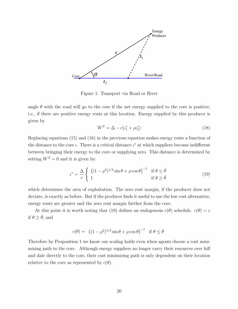
We assume the road is a straight line that crosses the core and expands indefinitely. The

location of a supplier relative to the core is described by two terms: ι, the distance from the

core and θ the angle between the segment formed by the core and the supplier and the road

as shown in Figure 1.

We solve the energy producer’s problem in two stages. In the first stage transportation

costs are minimized by choosing how much distance to cover by land and how much distance

to cover by river. In the second stage energy rents are maximized. The cost minimization

problem is given by:

minι1,ι2

cι1 + ρcι2 (13)

subject to

ι2 = ι21 − ι22 + 2ιι2 cos θ (14)

where ι1 is the distance travelled by land and ι2 is the distance travelled by road.

The constraint follows directly from the law of triangles with ι1 being opposite to the

angle θ, as shown in Figure 1. We can replace the constraint in the objective function to

find the optimal distances travelled by land and by road:

ι∗1 =ι sin θ

(1− ρ2)1/2(15)

and

ι∗2 = ι cos θ − ρι sin θ

(1− ρ2)1/2. (16)

If the distance ι∗2 is strictly positive, the supplier deviates to the road, otherwise the

supplier goes straight to the core. We can solve for the critical value of θ that separates the

suppliers that go straight to the core from those who deviate to the road:

ι∗2 > 0 if and only if θ ≤ cos−1 ρ ≡ θ (17)

Energy suppliers located at any angle θ < θ are “close” to the low cost alternative and

choose to use it. Since ρ = cos(θ) we know that as ρ → 0 everyone deviates, since it is so

cost effective. Alternatively, as ρ→ 1, the road offers no advantage and no one uses it.

The second part of the energy producer’s problem is to decide whether or not to take its

energy to the core. An energy producer situated a distance ι from the core and forming an

21ρ < 1 can alternatively represent the benefits of transmission at higher voltage, large cables, or bettermaterials.

19

River/Road Core

Energy Producer

ιι1

ι2θ

Figure 1: Transport via Road or River

angle θ with the road will go to the core if the net energy supplied to the core is positive;

i.e., if there are positive energy rents at this location. Energy supplied by this producer is

given by

W S = ∆− c(ι∗1 + ρι∗2) (18)

Replacing equations (15) and (16) in the previous equation makes energy rents a function of

the distance to the core ι. There is a critical distance ι∗ at which suppliers become indifferent

between bringing their energy to the core or supplying zero. This distance is determined by

setting W S = 0 and it is given by:

ι∗ =∆

c

{ ((1− ρ2)1/2 sin θ + ρ cos θ

)−1if θ ≤ θ

1 if θ ≥ θ(19)

which determines the area of exploitation. The zero rent margin, if the producer does not

deviate, is exactly as before. But if the producer finds it useful to use the low cost alternative,

energy rents are greater and the zero rent margin further from the core.

At this point it is worth noting that (19) defines an endogenous c(θ) schedule. c(θ) = c

if θ ≥ θ; and

c(θ) =((1− ρ2)1/2 sin θ + ρ cos θ

)−1if θ ≤ θ

Therefore by Proposition 1 we know our scaling holds even when agents choose a cost mini-

mizing path to the core. Although energy suppliers no longer carry their resources over hill

and dale directly to the core, their cost minimizing path is only dependent on their location

relative to the core as represented by c(θ).

20

3.2.2 The Magnification Effect

Just as before, the total energy supplied to the core is found by “adding up” all energy

rents.

W S = 4×

[∫ θ

0

∫ ι∗

0

v (∆− c (ι∗1 + ρι∗2)) dvdθ +

∫ π/2

θ

∫ ι∗

0

v (∆− cv) dvdθ

]

The first integral represents energy coming from suppliers who are close enough to the road

to use it in transport. The second integral represents the energy coming from those who

travel directly to the core. We have multiplied the integrals by 4 since we are adding up

over the quarter circles of π/2 radians.

Integrating and simplifying gives us a net energy supply much like that we had before:

W S =1

3

∆3

c2g(ρ) (20)

g(ρ) = π − 2θ + 2

∫ θ

0

((1− ρ2)1/2 sin θ + ρ cos θ

)−2dθ > 0 (21)

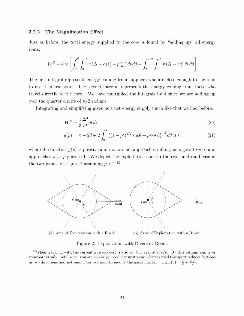
where the function g(ρ) is positive and monotonic, approaches infinity as ρ goes to zero and

approaches π as ρ goes to 1. We depict the exploitation zone in the river and road case in

the two panels of Figure 2 assuming ρ < 1.22

Road Core

θ

(a) Area of Exploitation with a Road

River Core θ

θ

(b) Area of Exploitation with a River

Figure 2: Exploitation with Rivers or Roads

22When traveling with the current a river’s cost is also ρc but against it c/ρ. By this assumption, rivertransport is only useful when you are an energy producer upstream; whereas road transport reduces frictions

in two directions and not one. Thus, we need to modify the gains function: griver(ρ) = π2 + g(ρ)

2 .

21

It is useful to redefine terms slightly to rewrite supply as:

W S =1

3

π∆3

c2where ∆ ≡ ∆(g(ρ)/π)1/3 and (g(ρ)/π)1/3 ≥ 1 (22)

which is exactly the same form as our earlier net supply with a slight redefinition of our

power density term. Importantly, because g(ρ) ≥ π we have proven:

Proposition 4 Magnification. Endowing our core with access to a low cost transportation

option is equivalent to endowing its surrounding region with more power dense energy re-

sources.

Proof. In text.

This result implies that as far as energy supply is concerned, having a road or river (or

transmission line) cut across the core is identical to being surrounded by more productive

energy resources.

Road location multiplies by some factor greater than one, the power density of available

resources. This multiplier depends on the cost reducing impact of the transportation option

as reflected in ρ. Setting ρ = 1 means the river or road offers no advantage in terms of

transportation. This implies g(ρ) = π since then θ = 0 and there is no multiplier of power

density. But any ρ < 1 effectively magnifies the power density of available resources; and

letting ρ approach zero implies g(ρ) approaches infinity and energy is no longer economically

scarce.

A moment’s reflection will reveal that regardless of the number, and regardless of the

efficacy of additional (straight line) transportation options we introduce, the endogenous

solution for energy supply delivered to the core, will again satisfy our scaling law. This is

true, since by Proposition 1 all cost minimizing paths are just different particular solutions

for c (θ). Moreover, if we were to add additional roads through our core these options can

only reduce costs (given optimization), and the equivalence result we report in Proposition 3

is strengthened. Every one of these additional transportation improvements is equivalent to,

in energy supply terms, an additional increase in the power density of surrounding resources.

With a small bit of work it can be shown that if we were to add any number of identical low

cost transportation options and locate them optimally, then:

Proposition 5 Energy supply to the core is an increasing and weakly concave function of

the number of transportation options serving it.

Proof. See Appendix.

The observable implication is that locations blessed with many transport options look

like they are endowed with very power dense energy resources.

22

3.3 Energy Investments

The magnification effect tells us two quite useful things. The first is that access to low

cost transport options is equivalent to raising the power density of surrounding resources.

Given this equivalence, for any investment lowering the physical cost of transport there is

an equivalent one raising the power density of energy resources by upgrading. Upgrading

resources and investing to lower transport costs are opposite sides of the same coin, and by

understanding the incentives for one we understand the incentives for both. Therefore we

consider only investments to lower transport costs in the text, and leave a similar parallel

analysis to footnotes where appropriate.

The second is that the marginal impact of low cost transport options is greater for

more power dense resources. This is apparent from (22) and it tells us the energy supply

consequences of say river access is far higher in a world run by, for example, coal than it

would be in one run on biomass. This suggests that investments to lower transport costs

will be greatest in situations where energy resources are already quite power dense.

To examine the motivation for energy investments assume the cost of building and main-

taining transport that delivers an efficiency of ρ is given by h(ρ).23 Assume ρ > ρ where ρ

is the minimum physically possible value of the coefficient of friction. Since a lower value of

ρ implies lower cost energy transport we assume h(ρ) is a decreasing and convex function:

h′(ρ) < 0 , h′′(ρ) > 0 with h(1) = 0 and h′(1) < 0. Then energy supplied net of infrastruc-

ture costs are WN = W S(ρ) − h(ρ). For concreteness consider the case where W S(ρ) is

given by equation (20) and we are improving river transportation by dredging, locks, canals,

maintaining ports etc. The optimal investment problem is simply given by

maxρWN = W S(ρ)− h(ρ) =

1

3

π∆3

c2g(ρ)− h(ρ) (23)

When the solution is interior, the first order condition that maximizes energy requires

1

3

π∆3

c2g′(ρ) = h′(ρ) (24)

23We could proceed in the same way to calculate the optimal investment on upgrading of resources. Up-grading resources is equivalent to increasing power density, ∆. Recall that for the case of renewables withmass we have ∆ = ed. The examples discussed above in the text suggest that the role of upgrading isincreasing energy content e, while taking concentration d as given. With this in mind, power supplied to the

core is given by WS(e, d) = 13πe3d(µg)2 . Next, consider a function k(e) such that k′(e) > 0 and k′′(e) > 0. k(e)

captures the costs of increasing the energy content of a resource. With this information, we can follow thesteps presented in (23) and (24) to show that improving transportation or upgrading resources (by increasingenergy content) are equivalent problems from the perspective of the energy producer.It also follows from the equivalence between electricity transmission lines and roads that increasing trans-mission voltage, therefore reducing Joule losses, is equivalent to reducing ρ which reduces land friction andtransportation loses.

23

The lefthand side of this equation is the marginal benefit from improved transport and it

is again a cubic in power density showing a strong relationship between power density and

the marginal benefit of further investments. The right hand side is simply marginal costs

of improved transportation. Since marginal benefits are bounded and marginal costs of the

first unit of investment are positive, with sufficiently low power density no investments in

transport improvements will occur. In situations with higher power density an interior

solution will obtain and we can write the implicit solution to (24) as ρ(∆). Straightforward

differentiation now shows24

dρ

d∆= − ρ

∆

3

ε′hρ − ε′gρ< 0

where ε′hρ = −ρh′′(ρ)/h′(ρ) and ε′gρ = −ρg′′(ρ)/g′(ρ) and the second order conditions sign

the expression.25 Therefore, we have proven:

Proposition 6 Complementarity. There exists a critical level of power density ∆c > 0 such

that for energy resources with ∆ < ∆c no investments in cost reducing transport occur; but

for environments with ∆ > ∆c, investment is positive and more power dense energy resources

call forth greater investments in cost reducing transportation investments.

Proposition 6 links the incentive for transport and upgrading of resources to their power

density. Resources with low power density will neither be upgraded nor call forth large in-

vestments to improve transportation. Biomass for example is not a very power dense energy

resource, and in a world run on biomass we should expect very local energy markets that

are severely constrained by transport costs. These local markets could be expanded some-

what by simple upgrading (charcoal), but the incentives for dedicated investments should

be weak. With the advent of fossil fuels new incentives arose. More power dense fuels like

coal brought forth large investments in lowering transport costs and upgrading. Canals,

railroads, and upgrading coal to coke could be seen as endogenous responses to its higher

power density. In the petroleum era we have witnessed and continue to witness today, mas-

sive investments in pipelines, tankers and terminals, so that the set of exploitable petroleum

resources now includes oil drilled in the world’s most inhospitable Arctic climates and is

collected from underwater wells literally miles deep. Naturally given the distances involved

24We have already assumed h′′(ρ) > 0; it can be shown that g(ρ) is convex for all values of ρ. The second

order conditions required for a maximum imply 13π∆3

c2 g′′(ρ) < h′′(ρ) which simply says the costs are moreconvex than the benefits from investing in infrastructure.

25For the case of resource upgrading, the optimization problem is given by maxeWN = WS(e, d)−k(e) =

13πe3d(µg)2 − k(e). The first order condition is given by πe2d

(µg)2 = k′(e). Finally we can totally differentiate the

first order condition to obtain: dedd = e/d

ε′ke−2 > 0, where ε′ke = ek′′(e)/k′(e) and the sign follows from the

assumption that costs are more convex than the benefits from upgrading resources.

24

and the distribution of resources around the world, energy shipments now routinely cross

political boundaries which has created a huge international trade in energy products where

two centuries previous there was virtually none at all. Proposition 6 links this long chain

of events to the changing power density of available energy sources.26

4 Empirical Application and Evaluation

The theory we developed makes several sharp predictions. To transfer these very abstract

predictions into their implications for empirical work it is useful to step back and examine

the role cheap energy plays in market economies.

The first effect is simply the direct impact cheap energy has on firm costs, production,

profits and, over the longer term, entry. If low energy costs are reliant on close proximity

to an energy source (because of transportation costs), then this direct impact will tend to

concentrate economic activity close to the cheap energy source. This is the concentration

motive, and it is the only motivation captured by our theory. Economic activity concentrated

in a region because of cheap energy, may however disappear if the original stimulus of cheap

energy is removed. Therefore, the concentration motive is potentially fleeting and surely will

be if the resource in question is non-renewable.

The second effect of cheap energy is agglomeration. If the original concentration of

activity leads to thick consumer, producer, and labor markets, then additional economic

activity may be stimulated as firms and laborers are attracted by the benefits thick markets

bring. In contrast to the concentration motive, the agglomeration of economic activity in a

region may be self sustaining long after the attraction of cheap energy is gone. Therefore

the agglomeration motive has potentially permanent effects.27

These observations imply that the distribution of economic activity we observe in the

world today may reflect a complex mix of these forces. They imply that cheap energy sources

from the distant past may have produced permanent centers of economic activity that today

are very distant from current energy supplies. In others cases, locally cheap energy resources

may have produced a boom and bust pattern of development, because agglomeration never

took hold. Since the world economy has employed many different energy sources, over many

centuries, we will have to identify a set of well documented case studies that trace through

the long run impacts of energy shocks.

26Notice that this analysis can be expanded to the case of electricity generation and transmission. Increas-ing voltages is costly but reduces line loses, therefore there is an incentive to invest for as long as the powerdelivered is enough to compensate for the investment in higher voltage lines.

27For a recent review of the relevant theory and empirics of agglomeration economies see Head and Mayer(2004)

25

If we are to use these case studies as litmus tests of our theory we should keep in mind

our theory’s three, potentially observable, implications. The first is our scaling law: holding

other features of a location constant (its access to rivers, roads, or transmission lines),

changes in the power density of available resources should produce large changes in energy

supply and, via the concentration motive, large changes in economic activity. The second

is our magnification effect. Access to low cost transportation options effectively magnifies

the energy resources available for use in the core: holding constant the energy resource in

question, variation in transport costs will create, via the concentration motive, large changes

in economic activity. The third is our finding of complementarity. The incentives to invest

in building infrastructure to lower the cost of transport is rising in the power density of

energy resources. Low density sources create no new investments; high density sources may

create extensive networks.

4.1 Introduction of the Lowly Potato

To uncover, and measure the strength of, the concentration motive it would be ideal if we

could observe a large energy shock where the underlying resource was very costly to transport

(implying the shock has a strong local impact); where its impact was geographically distinct

(giving us treatment and control units); and, where its transport costs remained high over

time (ensuring the impact had long term effects). Recent work by Nunn and Qian (2011)

linking the diffusion of the potato (a very power dense staple crop) to population and urban

growth in the Old World fits these requirements exactly.

Nunn and Qian (2011) provides empirical evidence linking the introduction of the potato,

from the New World to the Old, to higher population levels and urbanization rates in the Old

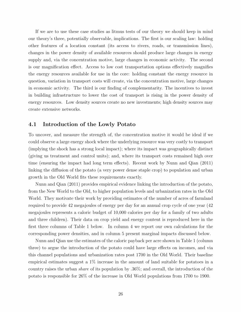
World. They motivate their work by providing estimates of the number of acres of farmland

required to provide 42 megajoules of energy per day for an annual crop cycle of one year (42

megajoules represents a caloric budget of 10,000 calories per day for a family of two adults

and three children). Their data on crop yield and energy content is reproduced here in the

first three columns of Table 1 below. In column 4 we report our own calculations for the

corresponding power densities, and in column 5 present marginal impacts discussed below.

Nunn and Qian use the estimates of the caloric payback per acre shown in Table 1 (column

three) to argue the introduction of the potato could have large effects on incomes, and via

this channel populations and urbanization rates post 1700 in the Old World. Their baseline

empirical estimates suggest a 1% increase in the amount of land suitable for potatoes in a

country raises the urban share of its population by .36%; and overall, the introduction of the

potato is responsible for 26% of the increase in Old World populations from 1700 to 1900.

26

Table 1: Crop Yields and Power Density

Crops Yield Energy Acres of land needed Power Increasedper acre Content to provide 42MJ per Density Powerkg MJ/kg day for one year W/m2 %

Wheat 650 13.69 1.7 .07 10.75Barley 820 13.90 1.4 .08 10.26Oats 690 13.47 1.6 .07 11.57Potatoes 10,900 2.92 0.5 .24 —

Notes: To obtain column 4 we transform 42MJ per day to Watts and Acres to meter. Suppose the numberin column 3 is Z acres per 42 MJ per day. Then we have 42MJ

Zacres−day = 42MJZacres−day ×

1day24∗60∗60sec ×

1acre4047m2

which canceling units is now in Watts/m2.

To obtain column 5 we use the numbers we found in column 4 and replace them in equation (25); where w

stands for wheat, oats, and barley and p for potato. Then we calculate the energy supplied by each of the

wold crops given by WSw =

π∆3w

3c2w. The number reported in column 5 is 1−WS

wp/WSw .

Their identification strategy exploits both the cross-sectional and time series variation in

the data by comparing population density in geographic units before and after the introduc-

tion of the potato, across units that are more or less, suitable for potato cultivation. This

is a perfect experimental design for examining our theory’s prediction that variation across

space in power density creates large impacts on energy supply and hence economic activity.

Table 1 provides evidence that potatoes are indeed a power dense energy source relative to

other staples; and their empirical results support Proposition 1’s prediction that the spatial

distribution of power dense energy resources can have large effects on the distribution of

economic activity.

While Nunn and Qian find large effects, are they too small for a world governed by our

scaling law? Column four shows the potato is at least three times more power dense than

competing staples. In a simple Malthusian set up where available energy per capita is fully

dissipated by population growth, we would expect a proportionate response in the population

to the change in net energy.28 If we combine these observations, should population have

grown by 33? Our theory suggests not. Only if the two crops yields (or d) are identical and

we are considering a complete replacement should net energy rise according to our scaling

law. Table 1 in fact shows the yield of potatoes is more than ten times higher than other

staples. Since staples are renewables with mass we have c = µgd and c2 is in the denominator

of (3). Using the figures from Table 1 and assuming the costs of transportation are similar

28For example, in the simplest Malthusian set up we would have population growth equal to births minusdeaths. Suppose births = b0 +b1(WS/L); deaths = d0−d1(WS/L); all parameters are positive and d0 > b0;then the steady state population is L = [(d1 + b1) / (d0 − b0)]WS and steady state population densities in aregion should be proportionate to net energy delivered by staples.

27

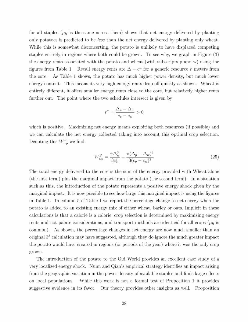
for all staples (µg is the same across them) shows that net energy delivered by planting

only potatoes is predicted to be less than the net energy delivered by planting only wheat.

While this is somewhat disconcerting, the potato is unlikely to have displaced competing

staples entirely in regions where both could be grown. To see why, we graph in Figure (3)

the energy rents associated with the potato and wheat (with subscripts p and w) using the

figures from Table 1. Recall energy rents are ∆ − cr for a generic resource r meters from

the core. As Table 1 shows, the potato has much higher power density, but much lower

energy content. This means its very high energy rents drop off quickly as shown. Wheat is

entirely different, it offers smaller energy rents close to the core, but relatively higher rents

further out. The point where the two schedules intersect is given by

r∗ =∆p −∆w

cp − cw> 0

which is positive. Maximizing net energy means exploiting both resources (if possible) and

we can calculate the net energy collected taking into account this optimal crop selection.

Denoting this W Swp we find:

W Swp =

π∆3w

3c2w

+π(∆p −∆w)3

3(cp − cw)2(25)

The total energy delivered to the core is the sum of the energy provided with Wheat alone

(the first term) plus the marginal impact from the potato (the second term). In a situation

such as this, the introduction of the potato represents a positive energy shock given by the

marginal impact. It is now possible to see how large this marginal impact is using the figures

in Table 1. In column 5 of Table 1 we report the percentage change to net energy when the

potato is added to an existing energy mix of either wheat, barley or oats. Implicit in these

calculations is that a calorie is a calorie, crop selection is determined by maximizing energy

rents and not palate considerations, and transport methods are identical for all crops (µg is

common). As shown, the percentage changes in net energy are now much smaller than an

original 33 calculation may have suggested, although they do ignore the much greater impact

the potato would have created in regions (or periods of the year) where it was the only crop

grown.

The introduction of the potato to the Old World provides an excellent case study of a

very localized energy shock. Nunn and Qian’s empirical strategy identifies an impact arising

from the geographic variation in the power density of available staples and finds large effects

on local populations. While this work is not a formal test of Proposition 1 it provides

suggestive evidence in its favor. Our theory provides other insights as well. Proposition

28

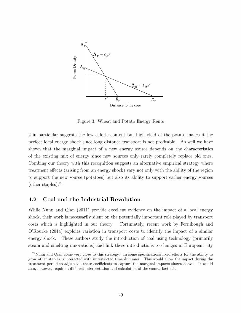
RW

ΔP

ΔW

RPr∗

ΔP − cPr

ΔW − cWr

Distance to the core

Pow

er D

ensi

ty

Figure 3: Wheat and Potato Energy Rents

2 in particular suggests the low caloric content but high yield of the potato makes it the

perfect local energy shock since long distance transport is not profitable. As well we have

shown that the marginal impact of a new energy source depends on the characteristics

of the existing mix of energy since new sources only rarely completely replace old ones.

Combing our theory with this recognition suggests an alternative empirical strategy where

treatment effects (arising from an energy shock) vary not only with the ability of the region

to support the new source (potatoes) but also its ability to support earlier energy sources

(other staples).29

4.2 Coal and the Industrial Revolution

While Nunn and Qian (2011) provide excellent evidence on the impact of a local energy

shock, their work is necessarily silent on the potentially important role played by transport

costs which is highlighted in our theory. Fortunately, recent work by Fernihough and

O’Rourke (2014) exploits variation in transport costs to identify the impact of a similar

energy shock. These authors study the introduction of coal using technology (primarily

steam and smelting innovations) and link these introductions to changes in European city

29Nunn and Qian come very close to this strategy. In some specifications fixed effects for the ability togrow other staples is interacted with unrestricted time dummies. This would allow the impact during thetreatment period to adjust via these coefficients to capture the marginal impacts shown above. It wouldalso, however, require a different interpretation and calculation of the counterfactuals.

29

populations during the Industrial Revolution.30 To do so the authors exploit both across city

variation in access to coal (by a distance to coal measure) and over time variation (before

and after the innovations diffused). They find that the ability to use coal (in these uses) was

responsible for over 60% of the growth in European city populations from 1750 and 1900.

Moreover, local access was found to be very important with a doubling of distance to coal

implying a 25% reduction in its impact on city populations. These are provocative new

results that again tie the location of new energy sources to subsequent growth in economic

activity, and they too provide largely supportive evidence for our theory. To move past

“largely supportive” to strong evidence in favor we need to demonstrate that coal is indeed

a very power dense resource; and secondly, that variation in transport costs are expected to

have large impacts in our theory.

To start consider transport costs. The authors exploit variation in a city’s distance to

coal to capture the intensity of treatment. In terms of our theory, their empirical design

corresponds to a situation where the type of energy is being held constant but distance

is being varied and this should impact energy supply. Given our CRS transport costs, a

doubling of distance to the core is equivalent, in energy rent terms, to a doubling of unit

costs c holding distance constant. And from (3), a doubling of c lowers net energy supply

four fold. Therefore, variation in the distance to energy works much like variation across

energy resources in power density. This general point was already apparent from our earlier

equivalence result and the resulting magnification effect.

Next consider coal’s power density. The method we presented earlier to calculate the

power density of renewables cannot be applied directly because non-renewables are obviously

very different. For example, the flow of energy obtained from non-renewables is proportional

to the change in the resource stock over time, and non-renewables are not spread over vast

areas but instead found in subsurface deposits of considerable thickness. To proceed we

deal with these issues in turn. First, assume the resource was distributed uniformly on the

surface of a two dimensional plane. Then the change in the resource stock would equal the

physical flow of the resource, which we will denote by φ[kg/m2·s], times the area exploited,

a[ m2]. This gives us the kilograms mined per second. Multiplying by energy content implies

the power density of a non-renewable resource distributed on the surface, could be written

30Moreno-Cruz and Taylor (2012) argue that the shift in England from biomass based fuels to coal in thelatter part of the sixteenth century was at least partially responsible for the radical shift in the populationdistribution across the country. In this earlier work we extend the Only Energy model to incorporate amotive for agglomeration coming from increased specialization. We then wed this model with Malthusianpopulation dynamics and migration to make both population size and its geographic distribution sensitiveto proximate energy resources in a county. Using this theory and simple statistics, we argue that access tothis very power dense energy resource altered the distribution of population across counties as the energytransition spread across England.

30

as:

W = eφa (26)

∆ = W/a = eφ (27)

This makes perfect sense: the flow of energy comes from the change in a stock; the magnitude

of the resulting energy flow is determined by the stock’s energy content; the change in the

stock is equal to the product of the area extracted times the physical flow of the resource

mined; and dividing by area exploited, we obtain the result. For future purposes it is also

useful to note that the zero rent margin for this non-renewable is again equal to R∗ = e/µg

since φ kg of the ore is being transported for each square meter mined per second; and hence

c = µgφ. Therefore, we have a quality/quantity result similar to Proposition 2.

Unfortunately, this measure of power density only holds in situations where non-renewables

are distributed very thinly across Earth’s surface. For example, shallow deposits of the

non-renewable peat may well fit this description. In the vast majority of cases however non-

renewables are not thinly distributed as surface deposits. To tackle this problem we need

to develop an appropriate measure of available resources in subsurface deposits. Energy re-

sources will be brought to the surface and then transported to the core only if they provide

positive energy rents; and this implies there is now an extensive margin of exploitation for

any mine in terms of depth. In the appendix we show resources at all depths above e/g

earn positive energy rents if brought to the surface; and these resources when brought to the

surface just represent, in essence, a greater density of energy resources at that point. It is

as if they are now surface resources that provide a flow φ per meter, and a power density ∆

as given below.

∆ = eφ where φ = edv/2g (28)

where e and g are as defined before, while dv is the volumetric density of the resource in

[kg/m3].

We now use this formula to calculate the power density for different types of coal in

Table 2 below. The formula above assumes a uniform distribution of resources, but in

reality deposits differ in terms of depth, quality of coal, and thickness. To give an idea of

the resulting power densities we present a set of alternative estimates. We present estimates

assuming a deposit’s thickness, h, is either 1 or 10 meters; estimates for deposit depths, h0,

of 0 and 10,000 meters; and since coal varies in quality due to the influence of time and

pressure we present estimates for a precursor (peat), low quality brown lignite coal; and

higher quality bituminous coal.

As shown, higher quality coal has both higher energy content and greater volumetric

31

Table 2: Power Density of Different Coals

Energy Volumetric Power Density [GW/m2]Resource Content Density h0=0 m h0=10000m

[MJ/kg] [kg/m3] h=1m h=10m h=1m h=10mAnthracite 33 1400 46.2 462 46.2 462Bituminous 33 913 30.1 301 30 300

Lignite 16 865 13.8 138 13.8 138Peat 14 310 4.34 43.4 4.31 43.1

Note: Data and construction shown in Appendix.

density. Time and pressure increase both and this implies given our formula that higher

quality coal is significantly more power dense than its precursor peat. We find the deposit

depth has little effect on the energy contained in the mine, and hence comparing the power

density of resources at zero depth versus those at 10,000 meters reveals only small differences.

And finally, the power densities are very large. To understand the scale of the energy shock

created by a movement to coal we compare these figures with similar figures for wood. We

use the methods developed previously for renewables and present in Table 3 estimates for a

set of representative forests. In particular, we use data on sustainably managed forests in

the United States. As shown, the power densities in Table 3 are very small, providing less

than one Watt of power (sustainably) per meter squared.

Table 3: Power Density of Wood

AverageForest Region Total Acres Ave. Prod. Percent Percent Power Dens.

(1,000s) (ft3/acre/yr) Softwood Hardwood (W/m2)Northeast 79,803 57.10 25.21% 74.79% 0.10North Central 84,215 66.54 18.72% 81.28% 0.12Southeast 85,665 80.22 41.00% 59.00% 0.14South Central 118,364 84.69 35.20% 64.80% 0.15Rocky Mountain 70,969 52.00 90.29% 9.71% 0.08Pacific Coast 75,197 81.71 89.01% 10.99% 0.12

Note: Data are shown in the Online Appendix.

Several observations are in order. First, a naive comparison of the figures in these tables

reveals large differences in power densities which naturally suggests the introduction of coal

would be a massive energy shock to an economy where wood provided most thermal energy.

While we believe that this was indeed the case, a comparison of these figures requires careful

attention. The power densities measured for renewables represents the flow of power we

capture on our one square meter of space ad infinitum. The wind blows, the sun shines,

crops grow and forests mature providing a potential, and constant in steady state, flow of

32

energy we can reap. In the case of non-renewables, the energy flow depends on how fast we

extract the resources contained in one square meter. A straight ahead comparison of power

densities across these tables implicitly assumes we are consuming all of the non-renewable

energy resources from one square meter (and all of its subsurface deposits) per second. This

is incredibly fast. A better interpretation of the differences in power densities across these

tables is that the potential for reaping power from non-renewables is just vastly greater.

A second observation is that any existing low cost transportation option has a bigger

impact on energy supplies when the resource is more power dense. This is an implication

of (22) which shows the magnification effect is larger for already power dense resources.

Therefore, existing rivers and roads would magnify the impact of coal far more than they

magnified the impact of biomass resources.

Third, any comparison of wood and coal using just energy contents will severely underes-

timate the impact of a move to coal. Coal offers perhaps 25 MJ/kg while wood 15 MJ/kg,

which means we would be willing to transport coal further than wood given similar transport

technologies, but not much further. But comparisons like these miss an important point

captured in the complementarity effect of Proposition 6. Because coal is so much more

power dense, the incentive for expanding the existing exploitation zone is much larger. And

it was these endogenous improvements (canals, railroads, ports) in response to coal that

combined with its power density to create a huge and long lasting energy shock.

Putting these findings together supports the view that new steam technologies and metal-

lurgical uses for coal would have unleashed a huge energy shock as Fernihough and O’Rourke

(2014) claim. The empirical findings show the impacts of coal were geographically distinct

given large transport costs, and the estimated changes in urbanization and populations are

again very large. However, since the observed changes in economic activity following a shock

of this magnitude will reflect both the direct changes created by the concentration motive,

plus the knock-on effects created by both complementary investment in transportation in-

frastructure and the impact of agglomeration, this work does not present evidence on the

strength of the concentration motive per se. It does however provide further evidence

that the spatial distribution of power dense energy resources can have large effects on the

distribution of economic activity.

4.3 Local Economies and Hydroelectricity

Neither of the contributions discussed so far divides the impact of “energy shocks” into that

caused by the concentration motive (which we model here) and that caused by agglomeration

motives (which we do not). However, the treatment periods in these studies cover hundreds

33

of years, and hence the impacts measured must surely reflect both the concentration and

agglomeration motives. In a very recent paper Severnini (2013) provides us with a method

to divide these overall impacts into their concentration and agglomeration components. Im-

portant for us is that Severnini’s estimates of the total impact arising from the concentration

motive alone is large. If a similar division were to hold for the impact of the potato and

coal, then the concentration motive for economic activity in those instances would also be

significant.

Severnini (2013) examines the impact of hydroelectric dam building on local communities

throughout the U.S from 1920 to 1980. A hydroelectric dam in a specific location represents a

very power dense energy source; and its placement is an energy shock much like those studied

by other authors. He exploits a recent study of hydro potential in the U.S. to develop an

experimental design where treated counties had dams built, whereas counties with equivalent

potential (but no dam) represent untreated counties. Using a sophisticated synthetic control

and event study methodology, he finds the impact of dams on county population growth is

considerable and long lasting.

One of the novel features of this study is that it compares the economic impact of dams

built before and after widespread access to high voltage transmission lines and thermal

generation. In a world without transmission capacity (or cheap thermal generation as a

substitute), a dam represents a purely local energy shock that creates both a concentration

motive and an agglomeration motive for economic activity.31 In a world with transmission

lines (and cheap thermal capacity), the local impact of the dam in terms of cheap power is

now dissipated by the opportunity to sell power in distant markets, and the ability to provide

competing power using thermal generation. As a result, a dam built post 1950 should have

little to no impact via the concentration motive and by implication spur no agglomeration.

By exploiting this logic, Severnini is able to divide the full economic impact of an energy

shock into the concentration and agglomeration motives. His estimates suggest that dams

built post 1950 produce very little new economic activity; dams built prior to 1950 provide

large gains (population density increased 51% over 30 years and 139% after 60 years for

counties treated with dams prior to 1950); but once we enter the post 1950s era with cheap

alternatives the benefits of a dam fall considerably. Using the pre and post 1950s growth for

treated counties, he estimates that approximately one half of the economic gains of a dam

is due to cheap local power or what we have called here the concentration motive.

Looking across all three studies, we find consistent evidence that proximity to a powerful

energy source creates large increases in economic activity. While many other studies have

31Indeed he provides evidence that the price of electricity was 45% lower in counties treated with a damrelative to control prior to 1950.

34

examined the correlation of existing resource stocks to trade flows, growth or other mea-

sures, what makes three studies examined here unique is their careful attention to issues of

causality. Each presents a clever experimental design combining both cross-sectional and

over time variation in unique ways to estimate the impact of energy shocks. While none

represent a formal test of our theory’s predictions, their results largely echo the three major

implications of our theory. Proximity and high power density drive the potato’s large im-

pact on populations; variation in distance and hence transport costs created the differential

impact of coal resources on subsequent European city growth; and the creation and then

removal of the advantages of cheap local power via hydro dams and transmission capacity

suggests that perhaps one half of the economic gains coming from an energy shock arise from

concentration motives alone.

5 Conclusions

This paper set out a simple spatial model in order to ask how the location and spatial

productivity of energy resources affects the distribution of economic activity around the

globe. This is a very large and as yet unanswered research question, and we have made an

admittedly modest but we think significant step towards its answer. Our major contribution

is the introduction of a new spatial approach to energy economics where elements from

both renewable and non-renewable resource economics are incorporated into a simple, albeit

stylized, model of energy use and production. This unity is provided by focussing on the

common output produced by both non–renewables and renewables - power- and by going

back to the fundamentals of work, force, power and resistance to understand at a very basic

level how physical differences across energy resources and their geographic location, can

affect deliveries of energy across space. The cost of this unity is that the reader is asked

to consider new terms, recall old definitions, and suffer through a seemingly obsessive focus

on units that is uncommon to most of economics. The benefits can be summed up in three

results: a scaling law, the magnification effect, and complementarity.

We find our spatial setting implies a scaling law. It implies that natural variation in the

spatial productivity of renewable energy resources will produce concentrations or bunching

in potential energy supplies at different locations. Even a uniform distribution across space

will generate a very skewed distribution of potential energy supplies across possible locations.

When energy comes from non-renewables, the scaling law implies a different type of bunching.

We find that all new non-renewable resource plays must first boom and then (optimally) bust,

which implies that extractions are now bunched in calendar time. In total the scaling law

tells us that concentrations in economic activity, either across space or across calendar time,

35

can arise for very simple reasons.

We find that roads, rivers and other low cost transportation options effectively magnify

the power density of available resources. This magnification effect can turn what appears

to be a resource poor region into a resource rich one. Therefore, having a road, river or

transmission line cross an economic core provides an energy supply equivalent to endowing

the region with far more power dense energy resources. Therefore, discrete natural variations

in geography like rivers, valleys and coastlines create their own magnification effects providing

an energy-centric explanation for much of the location of economic activity we see in the

world today.

Finally, while our energy system today is extremely complex and features an incredible

transport of energy from producers to consumers that suggests a focus on the locations

and productivity of energy resources may be misplaced, we turn this logic on its head by

showing how the incentive to create such an infrastructure relies on the existence of power

dense energy sources in the first place. By using ideal measures of power densities derived

from our theory we show that non-renewables are often 4 or 5 orders of magnitude more

power dense than renewables. The implication is that since purposeful investments in

transportation improvements and resource upgrading are complementary with resources of

greater power density, the fossil fuel era’s vast transportation network may be the cause of

the diaspora in economic activity we observe in the world today rather than its effect.

While our theoretical results are clear, the implications we have drawn for real world

data are both speculative and far reaching. Whether these implications are borne out by

future empirical work guided by our theory is impossible to know, but a simple litmus test

is available. At bottom all of these results hinge on there being strong relationships between

the power density of available resources, the supply conditions for energy they create, and

resulting economic activity (which we do not model). To address this deficiency we reviewed

three recent empirical studies which examined empirical relationships between the availability

of power dense energy resources, and the location of economic activity. These studies

examined both renewable and non-renewable energy sources, spanned nearly a millenia in

their observation periods, and each devised clever empirical strategies to reliably estimate a

causal relationship. While none offer a formal test our theory, we believe all provide strong

support for our overall approach.

36

6 References

Allen, Robert C. 2009. “The British Industrial Revolution in Global Perspective.” UK:

Cambridge University Press

Boyce, J.R. “Prediction and Inference in the Hubbert-Deffeyes Peak Oil Model.” The

Energy Journal, forthcoming.

Borenstein, S. J. Bushnell, and F. Wolak. 2002. “Measuring Market Inefficiencies in

California’s Restructured Wholesale electricity market.” The American Economic Review,

92(5): 1376-1405.

Chakravorty, U. and D.L. Kruice. 1994. “Heterogenous Demand and Order of Resource

Extraction.” Econometrica, 62(6): 1445-1452.

Chakravorty, U., J. Roumasset, and K. Tse. 1997. “Endogenous substitution among

energy resources and global warming.” Journal of Political Economy, 195: 1201-1234.

Fernihough, A. and K.H. O’Rourke. 2014. ”Coal and the European Industrial Revo-

lution”, National Bureau of Economic Research Working Paper No. 19802j.

Fouquet, R. and R. Pearson. 1998. “A Thousand Years of Energy Use in the United

Kingdom.” The Energy Journal, 19(4): 1-41.

Gaudet, G., M. Moreaux, and S.W. Salant. 2001. “Intertemporal Depletion of Re-

source Sites by Spatially Distributed Users.” American Economic Review, 91(4): 1149-1159.

Head, Keith and Thierry Mayer 2004. “The Empirics of Agglomeration and Trade”

Chapter 59 in Handbook of Regional and Urban Economics, Volume 4 edited by J.V. Hen-

derson and J.F. Thisse, Elsevier B.V.

Herfindahl, O.C. 1967. “Depletion in Economic Theory.” In Extractive Resources and

Taxation, edited by Mason Gaffney, 63-90. Madison, Wisconsin: University of Wisconsin

Press.

Holland, S.P. 2008. “Modeling Peak Oil.” The Energy Journal, 29(2): 61-79.

Hotelling, H. 1931. “The Economics of Exhaustible Resources.” Journal of Political Econ-

omy, 39(2): 137-175.

Joskow, P. and E. Kahn. 2002. “Quantitative Analysis of Pricing Behavior in California’s

Electricity Market During the Summer 2000.” The Energy Journal, 23(4): 1-35.

Kolstad, C.D. 1994. “Hotelling Rents in Hotelling Space: Product Differentiation in

Exhaustible Resource Markets.” Journal of Environmental Economics and Management,

26: 163-180.

Laffont, Jean-Jacques and Moreaux, Michel. 1986. “Bordeaux Contre Gravier: Une

Analyse par les Anticipations Rationnelles,” in Gerard Gaudet and Pierre Lasserre, eds.,

Ressources naturelles et theorie economique. Quebec: Presses de l’Universite Laval, 1986,

37

pp. 231- 53.

Livernois, J.R. and R.S. Uhler. 1987. “Extraction Costs and the Economics of Nonre-

newable Resources.” Journal of Political Economy, 95(11): 195-203.

Moreno-Cruz, J. and M.S. Taylor. 2012. “Back to the Future of Green Powered

Economies,” The National Bureau of Economic Research, Working Paper No: 18236.

Nordhaus, W. D. 2006. ”Geography and Macroeconomics: New Data and New Findings,”

Proceedings of the National Academy of Sciences (US), 103(10): 3510-3517.

Nunn, N. and N. Qian. 2011. “The Potato’s contribution to population and urbanization:

evidence from a historical experiment.” Quarterly Journal of Economics, 126, 593-650.

Pindyck, R.S. 1978. “The Optimal Exploration and Production of Nonrenewable Re-

sources.” Journal of Political Economy, 86(5): 841-861.

Severnini, E.R. ”The Power of Hydroelectric Dams: Agglomeration Spillovers”, Working

Paper at Carnegie Mellon University.

Salant, S. 1976. ”Exhaustible Resources and Industrial Structure: A Nash-Cournot Ap-

proach to the World Oil Market,” The Journal of Political Economy, 84(5): 1079-1093.

Sanchirico, J.N. and J.E. Wilen. 1999.“Bioeconomics of Spatial Exploitation in a Patchy

Environment.”Journal of Environmental Economics and Management, 37:129-150.

Smil, V. 2008. Energy in Nature and Society: General Energetics of Complex Systems.

USA: MIT Press.

Smulders, S. and E. van der Werf. 2008. “Climate policy and the optimal extraction

of high- and low-carbon fossil fuels,” Canadian Journal of Economics, 41(4):1421-1444.

Solow, R.M. and F.Y. Wan. 1976. “Extraction Costs in the Theory of Exhaustible

Resources.” The Bell Journal of Economics, 7(2): 359-370.

Swierzbinski, J.E. and Mendelsohn, R. 1989. “Exploration and Exhaustible Resources:

The Microfoundations of Aggregate Models.” International Economic Review, 30(1): 175-

186.

Wolfram, C.D. 1999. “Measuring Duopoly Power in the British Electricity Spot Market.”

The American Economic Review, 89(4): 805-826.

Wrigley, E.A. 2010. Energy and the English Industrial Revolution. Cambridge, U.K.:

Cambridge University Press.

38

A Proofs to Propositions

A.1 Proof to Proposition 1:

If transportation costs vary with the direction θ, then we can identify the maximum radius

in each direction θ as R(θ) = ∆c(θ)

. To show that gross power is homogeneous of degree 3 we

calculate the following integral:

W ∗ =

∫ 2π

0

∫ R∗(θ)

0

r∆drdθ =∆3

2

∫ 2π

0

1

c(θ)2dθ

which shows that for any function c(θ) gross power is a function homogeneous of degree 3 in

power density. To show the same is true for power supplied, we have to add the energy rents

∆− c(θ)r over all the farmers located a distance r away from the core in any direction θ.

W S =

∫ 2π

0

∫ R(θ)

0

r(∆− c(θ)r)drdθ =

∫ 2π

0

R(θ)2

2

(∆− 2

3R(θ)c(θ)

)dθ =

∆3

6

∫ 2π

0

1

c(θ)2dθ

This shows power supplied W S is homogeneous of degree three in power density, while the

precise form of the exploitation zone is determined by the form of c(θ).

A.2 Proof to Proposition 2:

A social planner maximizes the welfare of a representative consumer who values the energy

services available for consumption in the core. By choosing service units appropriately, utility

is defined over net energy supplied. The planner has a CRRA instantaneous utility function

with coefficient of relative risk aversion equal to σ > 0. Social welfare is:

maxW (t)

∫ ∞0

e−ρtU(W S(t))dt where U(W S) =(W S)1−σ − 1

1− σ(A.1)

The planner maximizes (A.1) subject to the constraints (6) and (7). We write the current

value Hamiltonian as

H = U [(1− C(X(t)))W (t)]− λ(t)W (t) (A.2)

where λ(t) is the co-state variable associated with the stock of resources. The optimality

conditions are given by:

∂H

∂W (t)= U ′(W S(t))(1− C(X(t)))− λ(t) = 0 (A.3)

39

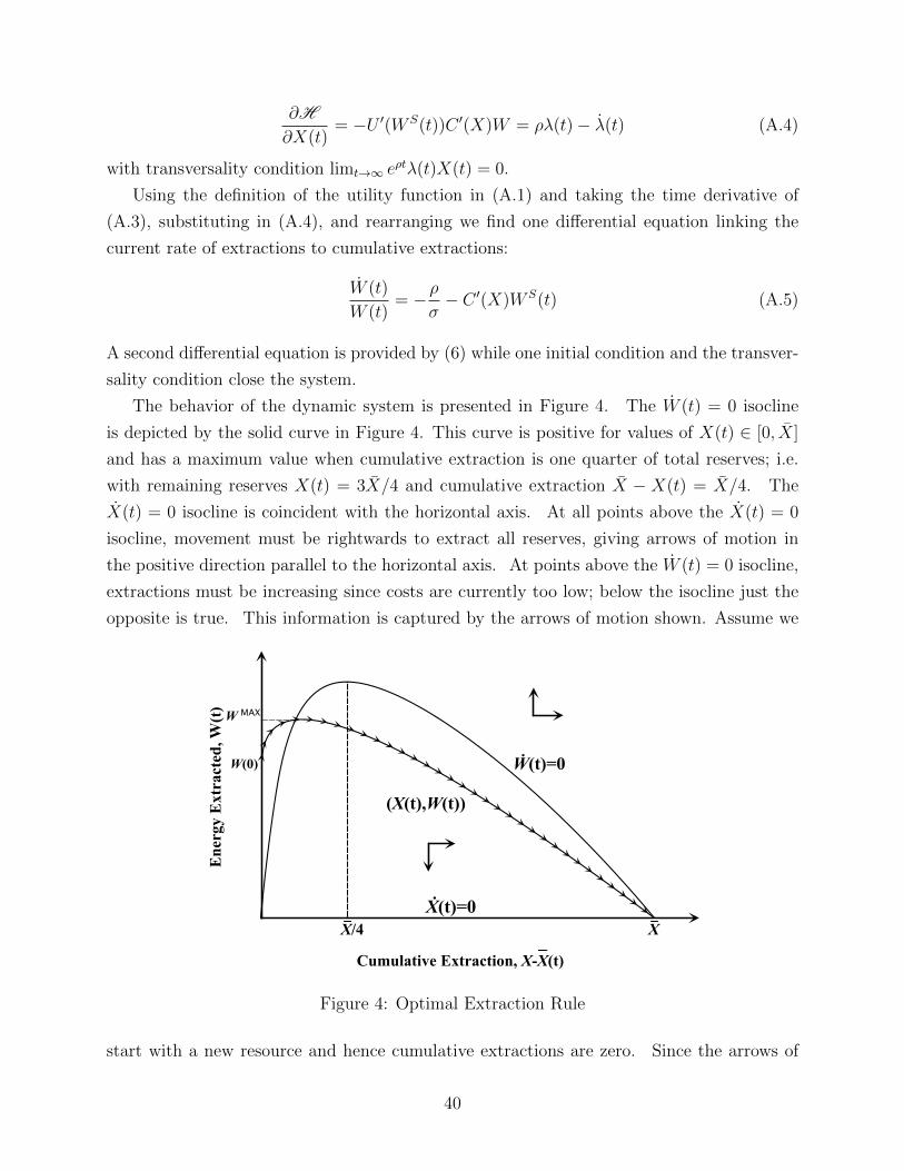
∂H

∂X(t)= −U ′(W S(t))C ′(X)W = ρλ(t)− λ(t) (A.4)

with transversality condition limt→∞ eρtλ(t)X(t) = 0.

Using the definition of the utility function in (A.1) and taking the time derivative of

(A.3), substituting in (A.4), and rearranging we find one differential equation linking the

current rate of extractions to cumulative extractions:

W (t)

W (t)= −ρ

σ− C ′(X)W S(t) (A.5)

A second differential equation is provided by (6) while one initial condition and the transver-

sality condition close the system.

The behavior of the dynamic system is presented in Figure 4. The W (t) = 0 isocline

is depicted by the solid curve in Figure 4. This curve is positive for values of X(t) ∈ [0, X]

and has a maximum value when cumulative extraction is one quarter of total reserves; i.e.

with remaining reserves X(t) = 3X/4 and cumulative extraction X − X(t) = X/4. The

X(t) = 0 isocline is coincident with the horizontal axis. At all points above the X(t) = 0

isocline, movement must be rightwards to extract all reserves, giving arrows of motion in

the positive direction parallel to the horizontal axis. At points above the W (t) = 0 isocline,

extractions must be increasing since costs are currently too low; below the isocline just the

opposite is true. This information is captured by the arrows of motion shown. Assume we

Cumulative Extraction, X-X(t)

Ene

rgy

Ext

ract

ed, W

(t)

Ẇ(t)=0

Ẋ(t)=0XX/4

W(0)

W MAX

(X(t),W(t))

Figure 4: Optimal Extraction Rule

start with a new resource and hence cumulative extractions are zero. Since the arrows of

40

motion near the origin imply all movement must be upwards and to the right, we know the

system must move immediately to an initial extraction point like that shown by W (0) = W0.

From this initial point, the arrows of motion indicate we move upwards and to the right and

cut the W (t) = 0 isocline at zero slope. Once we cross this isocline, the arrows of motion tell

us the extraction path must turn downwards and the transversality condition requires the

path slowly approach X on the horizontal axis. Working backwards it is now apparent the

transversality condition chooses the initial W0 and this choice has to feature less extraction

than that given by the peak of the W (t) isocline. This completes the proof that the optimal

extraction path first increases and then decreases.

Next, we show that the peak in the production path increases with power density. That

is, for any Z = X − X constant, WMAX is increasing in X. Setting dW/dX = 0 we find∂W∂X

= 2 ρσZ

(X1/2−Z1/2)− 12X1/2

(X1/2−Z1/2)2. Therefore, ∂W

∂X> 0 if X

4> (X −X) which always holds as the

peak in the extraction always occurs to the left of the peak in the W = 0 locus.

A.3 Proof to Proposition 5:

Assume all roads have the same coefficient of friction ρµ with 0 < ρ < 1. Optimal deployment

of the road system requires roads are built to maximize coverage. That is, roads will split

the space in equal parts. The first road, as we have assumed, would split the space in π

radians, then second road would split it in π/2 radians, the third road in π/3 radians, and

goes on as we increase the number of roads. Let n denote the number of roads. For given ρ,

if n < n where n ≡ π2 arccos(ρ)

then the exploitation zones added by each road do not overlap.

If n > n the exploitation zones will overlap. For n < n we have:

W S = 4×

[n

[∫ θ

0

∫ ι∗

0

v (∆− c (ι∗1 + ρι∗2)) dvdθ +

∫ π/2n

θ

∫ ι∗

0

v (∆− cv) dvdθ

]]

where we have exploited symmetry in the first quadrant of the cartesian space. The integral

is then given by:

W S =1

3

∆3

c2g(ρ, n), where g(ρ, n) = π − 2nθ + 2n

∫ θ

0

((1− ρ2)1/2 sin θ + ρ cos θ

)−2dθ

It is easy to see now that power supplied is linear in the number of roads, n. For n > n, the

exploitation zones will intersect at odd multiples of π/2n. The expression for power supplied

41

is now given by:

W S = 4×

[n

[∫ π2n

0

∫ ι∗

0

v (∆− c (ι∗1 + ρι∗2)) dvdθ

]]

W S =1

3

∆3

c2g(ρ, n), where g(ρ, n) = 2n

∫ π2n

0

((1− ρ2)1/2 sin θ + ρ cos θ

)−2dθ

To show that power supplied is increasing and concave in the number of transportation op-

tions when n > n we take derivatives with respect to n and show

∂WS

∂n= 2

3∆3

c2

[g(ρ,n)

2n− π

2n

((1− ρ2)1/2 sin π

2n+ ρ cos π

2n

)−2]> 0 and ∂2WS

∂n2 = −π3

(√1−ρ2 cos( π

2n)−ρ sin( π2n)

)4n5

(√1−ρ2 sin( π

2n)+ρ cos( π2n)

)3

which negative when√

1− ρ2 cos(π2n

)− ρ sin

(π2n

)> 0 or n > π

2 arccos(ρ).

B Unit Costs of Electricity Transmission

Electric power measured in Watts is equal to the product of voltage and current: W = V I

where V is voltage measure in Volts and I is current measured in Amperes. Volts times

Amperes is Watts and since the power flowing from any energy resource will be measured in

Watts we need to write line losses in these terms to find net power available for delivery to

the core.

When electricity is transmitted over any distance, the transmission line heats up as power

is lost to heat because of the line’s resistance (Joule heating). Resistance is in turn related to

the size, material and length of the line. Very simply resistance is given by R = (ρ/a)l where

ρ is a measure of the resistivity of the material used in the cable, a is the cross-sectional

area of the cable and l is its length. Therefore, losses due to resistance are simply linear

in distance much as frictional losses were linear in distance. To find the extent of losses

as a function of distance we need to transform line resistance (which is measured in Ohms)

into Watts. To do so we use another well known result from physics: Ohm’s law. This

law states that the current transmitted along a linear conductor is proportional to voltage

and inversely proportional to the resistance; that is, I = V/R. Using this law we can now

calculate the power dissipated by resistance. Denote the line losses from transmission by

WL. These losses can then be related to the voltage and amperage relevant to our line as

given by WL = V I. Now using Ohm’s law we can substitute out voltage (V = IR) to find

line losses WL are proportional to both resistance and the square of current since WL = I2R.

Replacing the expression for resistance we have WL = I2(ρ/a)l = cl; where c = I2(ρ/a).

42

C Measuring Power Density for Non-Renewables

Consider a hypothetical resource owner with resource rights to one meter squared of surface

area in our exploitation zone of homogenous resource quality. If this resource owner extracts

a 1m3 cube of energy resources with energy content e[J/kg] and volumetric density dv[kg/m3],

then this cubic meter has mass of dv[kg] and weight of dvg[N]. The total energy contained in

this cube would be simply edv[J] and if it was exhausted in one second the power delivered

would be edv [Watts].

Now consider resources contained beneath this 1m2. If resources are located at distance

η[m] from the surface, then the work needed to bring them to the surface would be just

gdvη[J] since work must be done to offset gravity. Energy rents in this case are just edv−gdvη.

Resources where the energy cost of extraction equals their entire energy content produce zero

energy rents and are located at depth η∗ = e/g. The net energy available must account for

the energy costs of extraction and is found by the following simple integration.

∆ =

η∗∫0

[edv − gdvη] dη =

∫ η∗

0

edv [1− (g/e)η] dη = e2dv/2g (C.1)

To calculate the power density of different deposits we suppose the upper limit of the

deposit is located at a distance h0 from the surface and the thickness of the deposit is h, so

the maximum depth of the deposit is h0 + h. Because the resource rights are over one meter

squared the dimensions of the deposit are simply h[m3]. In this case to measure the power

density of this deposit, we use:

∆ =

∫ min{h0+h,η∗}

h0

[edv − gdvη] dη = min{h [dve− gdv(h0 + h/2)] , e2dv/2g} (C.2)

43