1. - COnnecting REpositories · PDF fileBradley, Bowman and Griesenbeck, Journal of Choice Modelling, 3(1), ... receive the most attention are the use of tours in addition to trips

econstor www.econstor.eu

Der Open-Access-Publikationsserver der ZBW – Leibniz-Informationszentrum WirtschaftThe Open Access Publication Server of the ZBW – Leibniz Information Centre for Economics

Standard-Nutzungsbedingungen:

Die Dokumente auf EconStor dürfen zu eigenen wissenschaftlichenZwecken und zum Privatgebrauch gespeichert und kopiert werden.

Sie dürfen die Dokumente nicht für öffentliche oder kommerzielleZwecke vervielfältigen, öffentlich ausstellen, öffentlich zugänglichmachen, vertreiben oder anderweitig nutzen.

Sofern die Verfasser die Dokumente unter Open-Content-Lizenzen(insbesondere CC-Lizenzen) zur Verfügung gestellt haben sollten,gelten abweichend von diesen Nutzungsbedingungen die in der dortgenannten Lizenz gewährten Nutzungsrechte.

Terms of use:

Documents in EconStor may be saved and copied for yourpersonal and scholarly purposes.

You are not to copy documents for public or commercialpurposes, to exhibit the documents publicly, to make thempublicly available on the internet, or to distribute or otherwiseuse the documents in public.

If the documents have been made available under an OpenContent Licence (especially Creative Commons Licences), youmay exercise further usage rights as specified in the indicatedlicence.

zbw Leibniz-Informationszentrum WirtschaftLeibniz Information Centre for Economics

Bradley, Mark; Bowman, John L.; Griesenbeck, Bruce

Article

SACSIM: An applied activity-based model systemwith fine-level spatial and temporal resolution

Journal of Choice Modelling

Provided in Cooperation with:Journal of Choice Modelling

Suggested Citation: Bradley, Mark; Bowman, John L.; Griesenbeck, Bruce (2010) : SACSIM: Anapplied activity-based model system with fine-level spatial and temporal resolution, Journal ofChoice Modelling, ISSN 1755-5345, Vol. 3, Iss. 1, pp. 5-31

This Version is available at:http://hdl.handle.net/10419/66824

Journal of Choice Modelling, 3(1), pp. 5-31 www.jocm.org.uk

SACSIM: An applied activity-based model system with fine-level spatial and temporal resolution

Mark Bradley

1,* John L. Bowman

2,†Bruce Griesenbeck

3,Ŧ

1524 Arroyo Ave., Santa Barbara, CA 93109, USA

228 Beals Street, Brookline, MA 02446, USA

3Sacramento Area Council of Governments, 1415 L Street, Sacramento, CA, 95814 USA

Received 8 March 2008, revised version received 1 December 2009, accepted 7 December 2009

Abstract

This paper presents the regional travel forecasting model system (SACSIM) being used by the Sacramento (California) Area Council of Governments (SACOG). Within SACSIM an integrated activity-based disaggregate econometric model (DaySim) simulates each resident’s full-day activity and travel schedule. Sensitivity to neighborhood scale is enhanced through disaggregation of the modeled outcomes in three key dimensions: purpose, time, and space. Each activity episode is associated with one of seven specific purposes, and with a particular parcel location at which it occurs. The beginning and ending times of all activity and travel episodes are identified within a specific 30-minute time period. Within SACSIM, DaySim equilibrates iteratively with traditional traffic assignment models. SACSIM was calibrated and tested for a base year of 2000 and for forecasts to the years 2005 and 2035, and was subjected to a formal peer-review. It was used to provide forecasts for the Regional Transportation Plan (RTP) and continues to be used for various policy analyses.

The paper explains the model system structure and components, the integration with the traffic assignment model, calibration and validation, sensitivity tests, model application and Federal peer review results. We conclude that it is possible to create and apply a regional demand model system using parcel-level geography and half-hour time of day periods. Experiences thus far have pointed to major benefits of using detailed land use variables and urban design variables, but also to new challenges in providing parcel-level land use inputs for future years. Keywords: travel demand forecasting, activity-based models, microsimulation

* Corresponding author, T: +1 805-564 3908, [email protected] † T: +1 617-232 8189, [email protected] Ŧ T:+1 916- 340 6268, [email protected]

http://www.jocm.org.uk/

Bradley, Bowman and Griesenbeck, Journal of Choice Modelling, 3(1), pp. 5-31

6

1 Introduction

Over the last decade, activity-based travel demand microsimulation models have gradually gained acceptance in the U.S. as the eventual successor to conventional “four step” travel demand models for large metropolitan areas. Activity-based model systems have been applied in Portland (Bradley et al. 1998; Bradley et al. 1999), San Francisco (Bradley et al. 2001; Jonnalagadda et al. 2001), New York (Vovsha et al. 2002), Columbus (Vovsha et al. 2003), Dallas (Bhat et al. 2004), and Sacramento. Bradley and Bowman (2006) provide a detailed comparison of the properties of those model systems, as well as references to papers written about those models.

In 2009, additional activity-based model systems have reached various stages of development for Denver, Seattle, Bay Area, San Diego, Atlanta, Los Angeles and Phoenix. We have now reached the point where the majority of new travel demand model development projects for major metropolitan areas in the US are for activity-based model systems.

The innovative features of the new activity-based models systems that tend to receive the most attention are the use of tours in addition to trips as a basic unit of behavior, attention to how activities are generated and scheduled across an entire day, and, in some cases, how different household members interact to influence each others’ travel decisions. Another important aspect that tends to receive less attention is that using disaggregate micro-simulation of individual households and persons instead of the conventional aggregate zone-based framework provides the potential for much finer levels of spatial and temporal detail in the forecasts. To date, most of the applied activity-based models continued to rely on zones as the spatial level of detail, and to rely on four or five broad time periods of the day as the temporal level of detail. There has been some skepticism that the new activity-based model framework would be able to improve upon those typical levels of resolution.

The purpose of this article is to provide a detailed description of an operational activity-based model that takes advantage of the disaggregate microsimulation framework to provide much finer levels of resolution in forecasting. The Sacramento model system described below uses 48 half-hour time periods across the day as the basic units of temporal resolution, and uses individual parcels of land as the basic units of spatial resolution. This latter feature in particular is quite significant, given that a metropolitan area typically has over one million parcels, as compared to less than a few thousand traffic analysis zones. Using parcel-level resolution allows regional travel demand models to include land use variables and urban design variables at a level of detail that has not been possible in the past, allowing planners to look at wider range of land use and infrastructure policies, particularly those that affect non-motorized travel and accessibility to transit services.

2 SACSIM Model System Overview This paper presents a regional travel forecasting model system called SACSIM, implemented by the Sacramento (California) Area Council of Governments (SACOG). The system includes an integrated econometric microsimulation of personal activities and travel with a highly disaggregate treatment of the purpose, time of day and location dimensions of the modeled outcomes. SACSIM will be used for transportation and land development planning, and air quality analysis.

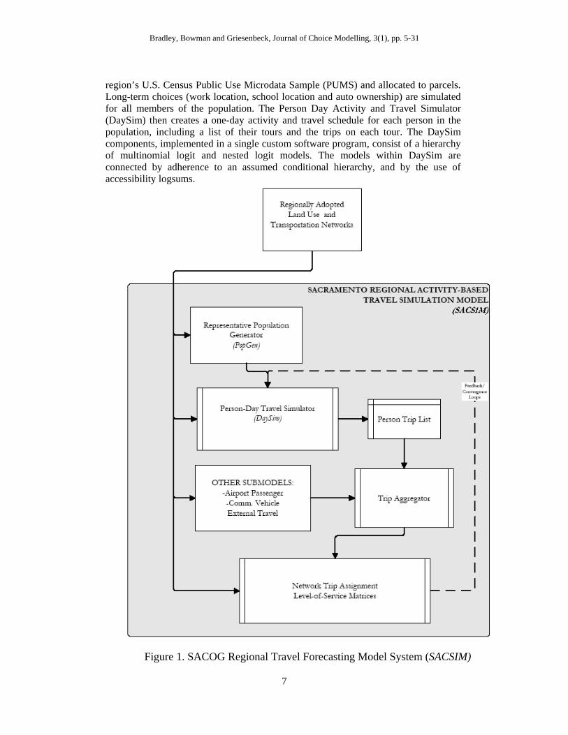
Figure 1 shows the major SACSIM components. The Representative Population Generator creates a synthetic population, comprised of households drawn from the


region’s U.S. Census Public Use Microdata Sample (PUMS) and allocated to parcels. Long-term choices (work location, school location and auto ownership) are simulated for all members of the population. The Person Day Activity and Travel Simulator (DaySim) then creates a one-day activity and travel schedule for each person in the population, including a list of their tours and the trips on each tour. The DaySim components, implemented in a single custom software program, consist of a hierarchy of multinomial logit and nested logit models. The models within DaySim are connected by adherence to an assumed conditional hierarchy, and by the use of accessibility logsums.

Figure 1. SACOG Regional Travel Forecasting Model System (SACSIM)

7


8

The trips predicted by DaySim are aggregated and combined with predicted airport passenger trips, external trips and commercial vehicle trips into time- and mode-specific trip matrices. The network traffic assignment models load the trips onto the network. Traffic assignment is iteratively equilibrated with DaySim and the other demand models.

As shown here, the regional forecasts are treated as exogenous. In subsequent implementations, it is anticipated that SACSIM will be fully integrated with PECAS, Sacramento’s new land use model (Abraham et al. 2004), so that the long range PECAS forecasts will depend on the activity-based travel forecast of DaySim.

2.1 DaySim Overview

DaySim follows the day activity schedule approach developed by Bowman and Ben-Akiva (2001). Its features include the following:

• The model uses a microsimulation structure, predicting outcomes for each household and person in order to produce activity/trip records comparable to those from a household survey (Bradley et al. 1999).

• The model works at four integrated levels—longer term person and household choices, single day-long activity pattern choices, tour-level choices, and trip-level choices

• The upper level models of longer term decisions and activity/tour generation are sensitive to network accessibility and a variety of land use variables.

• The model allows the specific work tour destination for the day to differ from the person’s usual work location.

• The model uses seven different activity purposes for both tours and intermediate stops (work, school, escort, shop, personal business, meal, social/recreation).

• The model predicts locations down to the individual parcel level. • The model predicts the time that each trip and activity starts and ends to the

nearest 30 minutes, using an internally consistent scheduling structure that is also sensitive to differences in travel times across the day (Vovsha and Bradley 2004).

• The model is highly integrated, including the use of mode choice logsums and approximate logsums in the upper level models, encapsulating differences across different modes, destinations, times of day, and types of person.

The latter four features are enhancements relative to its closest precursor, the CHAMP model currently in active use by the San Francisco County Transportation Authority (SFCTA). See Bradley et al. (2001) and Jonnalagadda et al. (2001) for details of the SFCTA model.

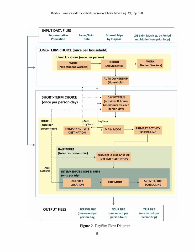
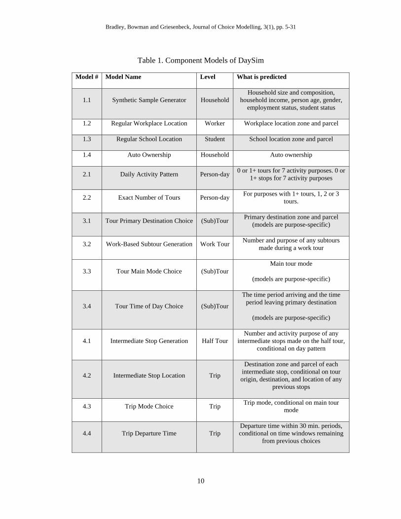
Figure 2 is a flow diagram showing the relationships among DaySim’s component models, which are also listed in Table 1. The models themselves are numbered hierarchically in the table; subsequently in this paper, parenthetical numerical references to models refer to these numbers. The hierarchy embodies assumptions about the relationships among simultaneous real world outcomes. In particular, outcomes from models higher in the hierarchy are treated as known in lower level models. It places at a higher level those outcomes that are thought to be higher priority to the decision maker. The model structure also embodies priority assumptions that are hidden in the hierarchy, namely the relative priority of outcomes


Figure 2. DaySim Flow Diagram

9


10

Table 1. Component Models of DaySim

Model # Model Name Level What is predicted

1.1 Synthetic Sample Generator Household Household size and composition,

household income, person age, gender, employment status, student status

1.2 Regular Workplace Location Worker Workplace location zone and parcel

1.3 Regular School Location Student School location zone and parcel

1.4 Auto Ownership Household Auto ownership

2.1 Daily Activity Pattern Person-day 0 or 1+ tours for 7 activity purposes. 0 or 1+ stops for 7 activity purposes

2.2 Exact Number of Tours Person-day For purposes with 1+ tours, 1, 2 or 3 tours.

3.1 Tour Primary Destination Choice (Sub)Tour Primary destination zone and parcel (models are purpose-specific)

3.2 Work-Based Subtour Generation Work Tour Number and purpose of any subtours made during a work tour

3.3 Tour Main Mode Choice (Sub)Tour Main tour mode

(models are purpose-specific)

3.4 Tour Time of Day Choice (Sub)Tour

The time period arriving and the time period leaving primary destination

(models are purpose-specific)

4.1 Intermediate Stop Generation Half Tour Number and activity purpose of any

intermediate stops made on the half tour, conditional on day pattern

4.2 Intermediate Stop Location Trip

Destination zone and parcel of each intermediate stop, conditional on tour origin, destination, and location of any

previous stops

4.3 Trip Mode Choice Trip Trip mode, conditional on main tour mode

4.4 Trip Departure Time Trip Departure time within 30 min. periods, conditional on time windows remaining

from previous choices


11

on a given level of the hierarchy. The most notable of these are the relative priority of tours in a pattern, and the relative priority of stops on a tour. The formal hierarchical structure provides what has been referred to by Vovsha et al. (2004) as downward vertical integrity.

Just as important as downward integrity is the upward vertical integrity that is achieved by the use of composite accessibility variables to explain upper level outcomes. Done properly, this makes the upper level models sensitive to important attributes that are known only at the lower levels of the model, most notably travel times and costs. It also captures non-uniform cross-elasticities caused by shared unobserved attributes among groups of lower level alternatives sharing the same upper level outcome.

Upward vertical integration is a very important aspect of model integration. Without it, the model system will not effectively capture sensitivity to travel conditions. However, when there are very many alternatives (millions in the case of the entire day activity schedule model), the most preferred measure of accessibility, the expected utility logsum, requires an infeasibly large amount of computation. So, for SACSIM approaches have been developed to capture the most important accessibility effects with a feasible amount of computation. One approach involves using logsums that approximate the expected utility logsum. They are calculated in the same basic way, by summing the exponentiated utilities of multiple alternatives. However, the amount of computation is reduced, either by ignoring some differences among decision makers, or by calculating utility for a carefully chosen subset or aggregation of the available alternatives. The approximate logsum is pre-calculated and used by several of the model components, and can be re-used for many persons. Two kinds of approximate logsums are used, an approximate tour mode/destination choice logsum and an approximate intermediate stop location choice logsum. The approximate tour mode-destination choice logsum is used in situations where information is needed about accessibility to activity opportunities in all surrounding locations by all available transport modes at all times of day. The approximate intermediate stop location choice logsum is used in the activity pattern models, where accessibility for making intermediate stops affects whether the pattern will include intermediate stops on tours, and how many.

The other simplifying approach involves simulating a conditional outcome. For example, in the tour destination choice model, where time-of-day is not yet known, a mode choice logsum is calculated based on an assumed time of day, where the assumed time of day is determined by a probability-weighted Monte Carlo draw. In this way, the distribution of potential times of day is captured across the population rather than for each person, and the destination choice is sensitive to time-of-day changes in travel level of service.

In many other cases within the model system, true expected utility logsums are used. For example, tour mode choice logsums are used in the tour time of day models.

3 Component Models of DaySim The models in the DaySim component of SACSIM were estimated using data from the 1999 Sacramento Area Household Travel Survey, fielded by NuStats. The survey was a fairly standard place-based one-day travel diary survey, very similar to most other regional household travel surveys carried out in the US during the last decade.

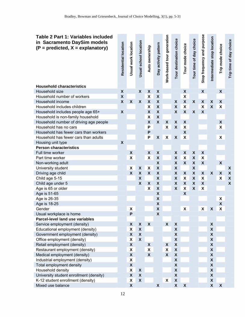
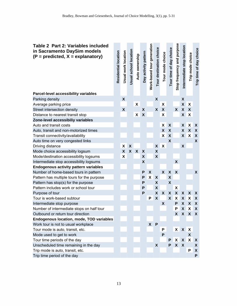
We do not have the space in this paper to provide details on the exact specification or estimation results for each component model. Table 2 provides a


12

Table 2 Part 1: Variables included in Sacramento DaySim models (P = predicted, X = explanatory)

Res

iden

tial l

ocat

ion

Usu

al w

ork

loca

tion

Usu

al s

choo

l loc

atio

n

Aut

o ow

ners

hip

Day

act

ivity

pat

tern

Wor

k-ba

sed

tour

gen

erat

ion

Tour

des

tinat

ion

choi

ce

Tour

mod

e ch

oice

Tour

tim

e of

day

cho

ice

Stop

freq

uenc

y an

d pu

rpos

e

Inte

rmed

iate

sto

p lo

catio

n

Trip

mod

e ch

oice

Trip

tim

e of

day

cho

ice

Household characteristics

Household size X X X X X X X Household number of workers X X X X Household income X X X X X X X X X X X Household includes children X X X X X X X Household includes people age 65+ X X X X X X X Household is non-family household X X Household number of driving age people X X X X X X Household has no cars P X X X X Household has fewer cars than workers P X Household has fewer cars than adults P X X X X X Housing unit type X Person characteristics Full time worker X X X X X X X Part time worker X X X X X X X Non-working adult X X X X X X University student X X X X X X X Driving age child X X X X X X X X X X X Child age 5-15 X X X X X X X X Child age under 5 X X X X X X X X Age is 65 or older X X X X X X Age is 51-65 X X Age is 26-35 X X Age is 18-25 X X Gender X X X X X X Usual workplace is home P X Parcel-level land use variables Service employment (density) X X X X X X Educational employment (density) X X X X Government employment (density) X X X X Office employment (density) X X X X Retail employment (density) X X X X X Restaurant employment (density) X X X X X Medical employment (density) X X X X X Industrial employment (density) X X X Total employment density X X X Household density X X X X University student enrollment (density) X X X X K-12 student enrollment (density) X X X X X Mixed use balance X X X X X X


13

Table 2 Part 2: Variables included in Sacramento DaySim models (P = predicted, X = explanatory)

Res

iden

tial l

ocat

ion

Usu

al w

ork

loca

tion

Usu

al s

choo

l loc

atio

n

Aut

o ow

ners

hip

Day

act

ivity

pat

tern

Wor

k-ba

sed

tour

gen

erat

ion

Tour

des

tinat

ion

choi

ce

Tour

mod

e ch

oice

Tour

tim

e of

day

cho

ice

Stop

freq

uenc

y an

d pu

rpos

e

Inte

rmed

iate

sto

p lo

catio

n

Trip

mod

e ch

oice

Trip

tim

e of

day

cho

ice

Parcel-level accessibility variables Parking density X X X Average parking price X X X X Street intersection density X X X X X X X Distance to nearest transit stop X X X X X Zone-level accessibiliy variables Auto and transit costs X X X X XAuto, transit and non-motorized times X X X X XTransit connectivity/availability X X X X XAuto time on very congested links X XDriving distance X X X X X Mode choice accessibility logsum X X X X X Mode/destination accessibility logsums X X X Intermediate stop accessibility logsums X X Endogenous activity pattern variables Number of home-based tours in pattern P X X X X XPattern has multiple tours for the purpose P X X X Pattern has stop(s) for the purpose P X X Pattern includes work or school tour P X X Purpose of tour P X X X X X X XTour is work-based subtour P X X X X X XIntermediate stop purpose X P X X XNumber of intermediate stops on half tour P X X XOutbound or return tour direction X X X XEndogenous location, mode, TOD variables Work tour is not to usual workplace X P Tour mode is auto, transit, etc. P X X X Mode used to get to work P X Tour time periods of the day P X X X XUnscheduled time remaining in the day X P X X XTrip mode is auto, transit, etc. P XTrip time period of the day P


14

summary of most of the explanatory variables used in the models. The reader is referred to the SACSIM Technical Memos (Bowman and Bradley 2005, 2006), available on the website http://JBowman.net, as well as the SACSIM07 Model Reference Report (SACOG 2008a). The following sections list some key aspects of the various DaySim component models. Similar models are grouped together, for ease of presentation. 3.1 Day Activity Pattern Model This model is a variation on the Bowman and Ben-Akiva approach, jointly predicting the number of home-based tours a person undertakes during a day for seven purposes, and the occurrence of additional stops during the day for the same seven purposes. The seven purposes are work, school, escort, personal business, shopping, meal and social/recreational. The pattern choice is a function of many types of household and person characteristics, as well as land use and accessibility at the residence and, if relevant, the usual work location. The main pattern model (2.1) predicts the occurrence of tours (0 or 1+) and extra stops (0 or 1+) for each purpose, and a simpler conditional model (2.2) predicts the exact number of tours for each purpose. The “base alternative” in the model is the “stay at home” alternative where all 14 dependent variables are 0 (no tours or stops are made).

Many household and person variables were found to have significant effects on the likelihood of participating in different types of activities in the day, and on whether those activities tend to be made on separate tours or as stops on complex tours. The significant variables include employment status, student status, age group, income group, car availability, work at home dummy, gender, presence of children in different age groups, presence of other adults in the household, and family/non-family status. For workers and students, the accessibility (mode choice logsum) of the usual work and school locations is positively related to the likelihood of traveling to that activity on a given day. For workers, the accessibility to retail and service locations on the way to and from work is positively related to the likelihood of making intermediate stops for various purposes.

Simpler models were estimated to predict the exact number of tours for any given purpose, conditional on making 1+ tours for that purpose. An interesting result is that, compared to the main day pattern model, the person and household variables have less influence but the accessibility variables have more influence. This result indicates that the small percentage of people who make multiple tours for any given purpose during a day tend to be those people who live in areas that best accommodate those tours. Other people will be more likely to participate in fewer activities and/or chain their activities into fewer home-based tours.

The DaySim models implemented in Sacramento do not include explicit models of intra-household interactions. Although explanatory variables are used throughout the model system to take account of the characteristics of other household members, we do not explicitly link the activity patterns across individuals so that they travel together. During the period that the Sacramento model system was being developed, the first such applied intra-household interaction models of that type were being developed and applied for the Columbus and Atlanta regions. For Sacramento, on the other hand, the focus was placed on using finer level spatial detail (parcels) and temporal detail (30 minute periods), as well as on achieving upward integrity through consistent use of accessibility logsums at all levels of the model system. Adding

http://jbowman.net/


15

models of explicit intra-household interactions may be a worthwhile additional during future model update projects (along with other potential improvements described in the final section of this paper).

3.2 Generation Model for Work-based Subtours For this model, the work tour destination is known, so variables measuring the number and accessibility of activity opportunities near the work site influence the number and purpose of work-based tours. This model is very similar in structure to the stop participation and purpose models described next.

3.3 Generation Model for Intermediate Stops on Half-Tours For each tour, once its destination, timing and mode have been determined, the exact number of stops and their purposes is modeled for the half-tours leading to and from the tour destination. For each potential stop, the model predicts whether it occurs or not and, if so, its activity purpose. This repeats as long as another stop is predicted. The outcomes of this model are strongly conditioned by (a) the outcome of the day activity pattern model, and (b) the outcomes of this model for higher priority tours. For the last modeled tour, this model is constrained to accomplish all intermediate stop activity purposes prescribed by the activity pattern model that have not yet been accomplished on other tours.

The estimation results for this model indicate that accessibility measures are important in determining which stops are made on which tours, as well as the exact number of stops. An important feature of this model system is that we do not predict the number and allocation of stops completely at the upper pattern level, as is done in the Portland and SFCTA models, or completely at the tour level, as is done in other models such as those in Columbus and New York. Rather, the upper level pattern model predicts the likelihood that ANY stops will be made during the day for a given purpose, at a level where the substitution between extra stops versus extra tours can be modeled directly. Then, once the exact destinations, modes and times of day of tours are known, the exact allocation and number of stops is predicted using this additional tour-level information. We think that this approach provides a good balance between person-day-level and tour-level sensitivities.

3.4 Location Choice Models 3.4.1 Usual Work and School Locations and Tour Primary Destinations The dependent variable in the usual location and tour destination models is the parcel address where the activity takes place. Since over 700,000 parcels comprise the universal set of location choice alternatives in the SACOG six-county region, it is necessary to both estimate and apply the location choice models using a sample of alternatives. The sampling of alternatives is done using two-stage importance sampling with replacement; first a TAZ is drawn according to a probability determined by its size and impedance, and then a parcel is drawn within the TAZ, with a size-based probability.


16

Some differences among the models come from the assumed model hierarchy in Table 2.For the usual work and school location models, auto ownership is assumed to be unknown, based on the assumption that auto ownership is mainly conditioned by work and school locations of household members, rather than the other way around. For the tour destinations, auto ownership levels are treated as given, and affect location choice. For university and grade school students who also work, the usual school location is known when usual work location is modeled; for other workers who also go to school, the work location is known when usual school location is modeled. For the tour destination models, all usual locations are known.

There are additional structural differences among these models. For the two usual location models (work and school), the home location is treated as a special location, because it occurs with greater frequency than any given non-home location, and size and impedance are not meaningful attributes. As a result, both of these models take the nested logit form, with all non-home locations nested together under the conditioning choice between home and non-home. In the estimation data, all workers have a usual work location and all students have a usual school location, so the model does not have an alternative called “no usual location”.

Because a large majority of work tours go to the usual work location, the work tour destination model has this as a special alternative. Therefore, the model is nested, with all locations other than the usual location nested together under the conditioning binary choice between usual and non-usual. (Nearly all observed school tours go to the usual school location. Therefore, there is no school tour destination choice model.)

Since there are no modeled usual locations for activities other than work and school, the destination choice model of all remaining purposes is simply a multinomial logit model.

Two important variables in all of these models are the disaggregate mode choice logsum and network distance. The logsum represents the expected maximum utility from the tour mode choice, and captures the effect of transportation system level of service on the location choice. Distance effects, independent of the level of service, are also present to varying degrees depending on the type of tour being modeled. In nearly all cases, sensitivity to distance declines as distance increases; in some cases this is captured through a logarithmic form of distance. In other cases, where there is plenty of data to support a larger number of estimated parameters, a piecewise linear form is used to more accurately capture this nonlinear effect.

In most cases the models include an aggregate mode-destination logsum variable at the destination. A positive effect is interpreted as the location’s attractiveness for making subtours and intermediate stops on tours to this location. A mix of parking and employment, at both the zone and parcel level, as well as street connectivity in the neighborhood, attract workers and tours for non-work purposes. Also, parcel-based size variables and TAZ-level density variables affect location choice.

3.4.2 Locations of Intermediate Stops For intermediate stop locations, the main mode used for the tour is already known, and so are the stop location immediately toward the tour destination (stop origin), and the tour origin. So the choice of location involves comparing, among competing locations, (a) the impedance of making a detour to get there, given the tour mode, and (b) the location’s attractiveness for the given activity purpose. The model is a multinomial logit (MNL).


17

Trip characteristics used in the model include stop purpose, tour purpose, tour mode, tour structure, stop placement in tour, person type, and household characteristics. The most important characteristics are the tour mode and the stop purpose. The tour mode restricts the modes available for the stop, and this affects the availability and impedance of stop locations. The availability and attractiveness of stop locations depend heavily on the stop purpose. Tour characteristics also affect willingness to travel for the stop, and the tendency to stop near the stop or tour origin. These trip and tour characteristics tend to overshadow the effect of personal and household characteristics in this model.

The main impedance variable is generalized time, as well as its quadratic and cubic forms, to allow for nonlinear effects. It combines all travel cost and time components according to assumptions about their relative values. Generalized time is used, instead of various separately estimated time and cost coefficients, because the intermediate stop data is not robust enough to support good estimates of the relative values. Generalized time is measured as the (generalized) time required to travel from stop origin to stop location and on to tour origin, minus the time required to travel directly from stop origin to tour origin. It is further modified by discounting it according to the distance between the stop origin and the tour origin. The discounting is based on the hypothesis that people are more willing to make longer detours for intermediate stops on long tours than they are on short tours.

Additional impedance variables used in the model include travel time as a fraction of the available time window, which captures the tendency to choose nearby activity locations if there are tight time constraints on the stop, and proximity variables (inverse distance), which capture the tendency to stop near either the stop origin or the tour origin.

3.5 Mode Choice Models 3.5.1 Tour Main Mode

The tour mode choice model determines the main mode for each tour (a small percentage of tours are multi-modal), There are eight modes, although some of them are only available for specific purposes. They are listed below along with the availability rules, in the same priority order as used to determine the main mode of a multi-mode tour:

1. Drive to Transit: Available only in the Home-based Work model, for tours with a valid drive to transit path in both the outbound and return observed tour

2. Walk to Transit: Available in all models except for Home-based Escort, for tours with a valid walk to transit path in both the outbound and return observed tour periods.

3. School Bus: Available only in the Home-based School model, for all tours. 4. Shared Ride 3+: Available in all models, for all tours. 5. Shared Ride 2: Available in all models, for all tours. 6. Drive Alone: Available in all models except for Home-based Escort, for tours

made by persons age 16+ in car-owning households. 7. Bike: Available in all models except for Home-based Escort, for all tours with

round trip road distance of 30 miles or less. 8. Walk: Available in all models, for all tours with round trip road distance of 10

miles or less.


18

Transit has less than 1 percent mode share and Bicycle has less than 2 percent mode share for all purposes except Work and School. In order to get enough transit and bicycle tours to provide reasonable estimates, the home-based non-mandatory purposes of shopping, personal business, meal and social/recreation were grouped in a single model, but using purpose-specific dummy variables to allow for different mode shares for different purposes.

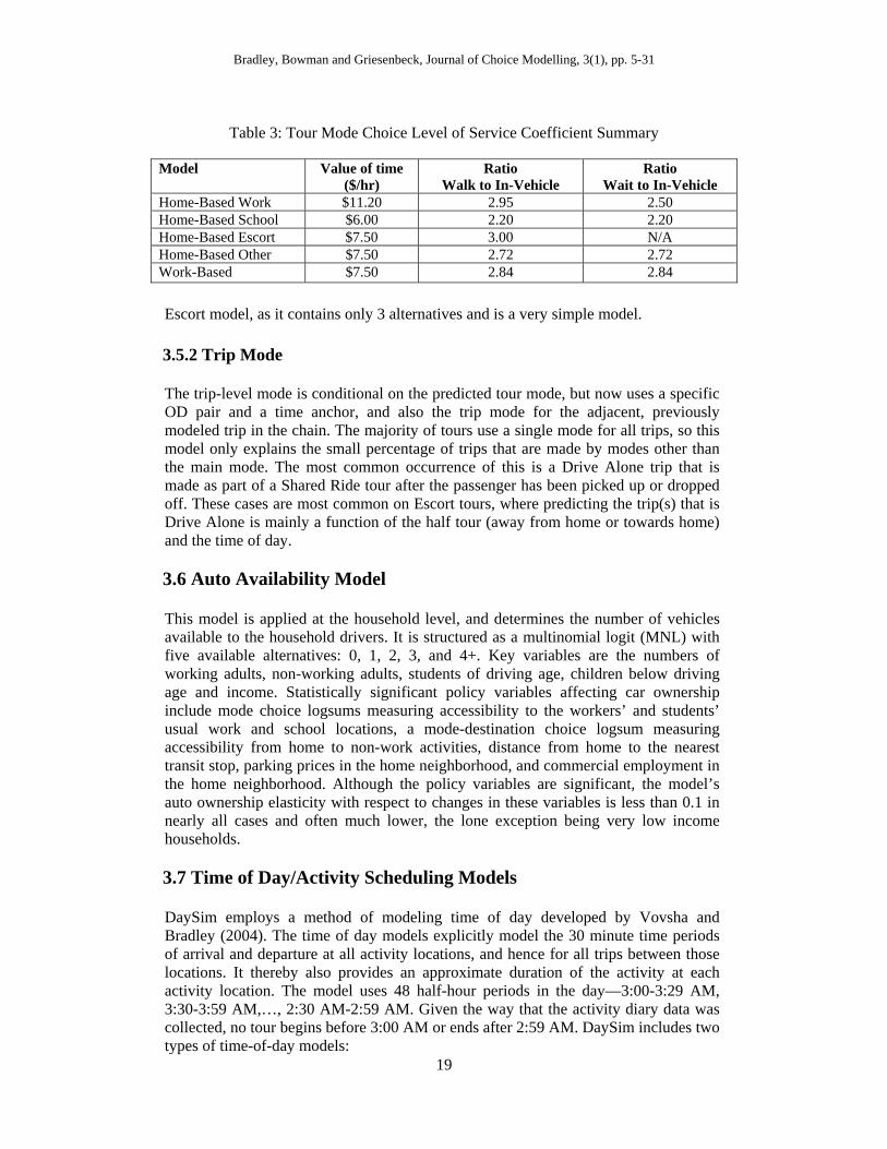
In general, it was possible to obtain significant coefficients for out-of-vehicle times, but not for travel costs or in-vehicle times. This is a typical result for RP data sets, particularly when there are few transit observations. As a result, many of the coefficients for cost and in-vehicle time were constrained at values that met the following criteria: (1) the in-vehicle time coefficients meet the United States Federal Transit Administration (FTA) guidelines, (2) the imputed values of time are reasonable and meet FTA guidelines, and (3) the values were kept as close as possible to what the initial estimation indicated. The resulting values of time and out-of-vehicle/in-vehicle time ratios are shown in Table 3. The number of transfers was not found to be significant in any of the models, however transfer wait time is included in the out-of-vehicle time coefficients. Also, the higher the percentage of time in a Drive to Transit path that is spent in the car rather than on transit, the lower the probability of choosing it. This is a result often found in other cities as well, which serves to discourage park-and-ride choices that include long drives followed by short transit rides.

Two land use variables came out as significant in many of the models, increasing the probability of walk, bike and transit:

Mixed use density: This is defined as the geometric average of retail and service employment (RS) and households (HH) within a half mile of the origin or destination parcel (= RS × HH / (RS + HH)). This value is highest when jobs and households are both high and balanced. High values near the tour origin tend to encourage walking and biking, while high values near the tour destination more often encourage transit use. Intersection density: This is defined as the number of 4-way intersections plus one half the number of 3-way intersections minus the number of 1-way “intersections” (dead ends and cul de sacs) within a half mile of the origin or destination parcel. Higher values tend to encourage walking for School and Escort tours, where safety for children is an issue, and also to encourage walking, biking and transit for Home-Based Other tours. A number of different nesting structures were tested. In the nesting structure that was selected there are three combined nests:

(1) Drive to Transit with Walk to Transit (2) Shared Ride 2 with Shared Ride 3+ (3) Bike with Walk

These all gave logsum coefficients less than 1.0 but not significantly different from each other, so a single estimated nesting parameter applies to all 3 nests (as well as to the 2 additional “nests” that only have one alternative each: Drive Alone, and School Bus). The estimated logsum parameters are 0.51 for Work, 0.86 for School, and 0.73 for Other. For Work-Based tours, it was not possible to obtain a stable estimate, so a constrained value of 0.75 (similar to HBOther) was used. No nesting was used for the


19

Table 3: Tour Mode Choice Level of Service Coefficient Summary

Model Value of time ($/hr)

Ratio Walk to In-Vehicle

Ratio Wait to In-Vehicle

Home-Based Work $11.20 2.95 2.50 Home-Based School $6.00 2.20 2.20 Home-Based Escort $7.50 3.00 N/A Home-Based Other $7.50 2.72 2.72 Work-Based $7.50 2.84 2.84 Escort model, as it contains only 3 alternatives and is a very simple model. 3.5.2 Trip Mode The trip-level mode is conditional on the predicted tour mode, but now uses a specific OD pair and a time anchor, and also the trip mode for the adjacent, previously modeled trip in the chain. The majority of tours use a single mode for all trips, so this model only explains the small percentage of trips that are made by modes other than the main mode. The most common occurrence of this is a Drive Alone trip that is made as part of a Shared Ride tour after the passenger has been picked up or dropped off. These cases are most common on Escort tours, where predicting the trip(s) that is Drive Alone is mainly a function of the half tour (away from home or towards home) and the time of day.

3.6 Auto Availability Model This model is applied at the household level, and determines the number of vehicles available to the household drivers. It is structured as a multinomial logit (MNL) with five available alternatives: 0, 1, 2, 3, and 4+. Key variables are the numbers of working adults, non-working adults, students of driving age, children below driving age and income. Statistically significant policy variables affecting car ownership include mode choice logsums measuring accessibility to the workers’ and students’ usual work and school locations, a mode-destination choice logsum measuring accessibility from home to non-work activities, distance from home to the nearest transit stop, parking prices in the home neighborhood, and commercial employment in the home neighborhood. Although the policy variables are significant, the model’s auto ownership elasticity with respect to changes in these variables is less than 0.1 in nearly all cases and often much lower, the lone exception being very low income households. 3.7 Time of Day/Activity Scheduling Models

DaySim employs a method of modeling time of day developed by Vovsha and Bradley (2004). The time of day models explicitly model the 30 minute time periods of arrival and departure at all activity locations, and hence for all trips between those locations. It thereby also provides an approximate duration of the activity at each activity location. The model uses 48 half-hour periods in the day—3:00-3:29 AM, 3:30-3:59 AM,…, 2:30 AM-2:59 AM. Given the way that the activity diary data was collected, no tour begins before 3:00 AM or ends after 2:59 AM. DaySim includes two types of time-of-day models:


20

3.7.1 Tour Primary Destination Arrival and Departure Time For each home-based or work-based tour, the model predicts the time that the person arrives at the tour primary destination, and the time that the person leaves that destination to begin the return half-tour. The tour model includes as alternatives every possible combination of the 48 alternatives, or 48×49 / 2 = 1,716 possible alternatives. The model is applied after the tour primary destination and main mode have already been predicted. Since entire tours, including stop outcomes, are modeled one at a time, first for work and school tours and then for other tours, the periods away from home for each tour become unavailable for subsequently modeled tours.

3.7.2 Intermediate Stop Arrival or Departure Time For each intermediate stop made on any tour, this model predicts either the time that the person arrives at the stop location (on the first half tour), or else the time that the person departs from the stop location (on the second half tour). On the second (return) half tour, we know the time that the person departs from the tour primary destination, and, because the model is applied after the stop location and trip mode have been predicted, we also know the travel time from the primary destination to the first intermediate stop. As a result, we know the arrival time at the first intermediate stop, so the model only needs to predict the departure time from among a maximum of 48 alternatives (the same 30 minute periods that are used in the tour models). This procedure is repeated for each intermediate stop on the half tour. On the first (outbound) half tour, the stops are simulated in reverse order from the primary destination back to the tour origin, so we know the departure time from each stop and only need to predict the arrival time. As stops within a tour are modeled, the periods occupied by each modeled stop become unavailable for subsequently modeled stops and tours.

A key concept in the time of day models is the “time window”. A time window is a set of contiguous time periods that are available for scheduling tours and stops. When a tour or stop is scheduled, the portion of the window that it does not fill is left as two separate and smaller time windows. The time periods at either end of a scheduled sequence of activities on a tour are only partially filled, but the time periods in between are completely filled. It is possible to arrive at a tour or stop destination in a given time period if another tour ended in that period, and possible to leave a tour or stop destination if another tour began in that period, but it is not possible to arrive or depart in a time period that is already completely filled.

Another key aspect is the use of shift variables. These are dummy variables interacted with the arrival time and the duration of the alternative. If the arrival shift coefficient is negative, it means that activities tend to be made earlier (because the shift coefficient causes later arrival time alternatives to have lower utility), and if it is positive, it means that activities tend to be made later. If the duration shift coefficient is negative, it means that activities tend to be shorter (because the shift coefficient causes longer duration time alternatives to have lower utility), and if it is positive, activities tend to be longer. No departure shift coefficient is estimated because the departure shift is simply the sum of the arrival shift and the duration shift (e.g. if the arrival shift is an hour earlier and the duration shift is an hour longer, the departure shift is 0). In the models, shift variables interact extensively with other characteristics of the person, day activity pattern and tour, as well as time-dependent attributes of the


21

network, such as travel times and measures of congestion, to effectively represent their influence on time-of-day choice.

The time of day models also use a variety of variables to represent scheduling pressure, conditional on what other activities have already been scheduled or remain to be scheduled for the day. The overall scheduling pressure is given by the number of tours remaining to be scheduled divided by the total empty window that would remain if an alternative is chosen. The negative effect indicates that people are less likely to choose schedule alternatives that would leave them with much to schedule and little time to schedule it in. A similar variable is the number of tours remaining divided by the maximum consecutive time window. This is also negative, meaning that people with more tours to schedule will tend to try to leave a large consecutive block of time rather than two or more smaller blocks.

Relative travel times across the day also influence time of day choice. The travel time for each period is based on the network travel times for the 4 periods of the day – AM peak, midday, PM peak, and off-peak. The variable is applied for both the outbound half tour (tour origin to tour destination) and the return half (tour destination to tour origin). For auto tours, the time is just the in-vehicle time, while transit time is in-vehicle time plus first wait time, transfer time, and drive access time. Walk access/egress time is not included, as that does not vary by time period. These variables are not applied for walk, bike or school bus tours. Significant travel time effects were found for Work and Other tours and for Intermediate Stops, but not for School or Work-based Tours.

Auto congestion may also cause time shifts within the AM peak and PM periods. For this purpose, the variable used was the extra time spent on links where the congested time is over 20 percent higher than the free flow time. This extra congested time was converted to shift variables by multiplying by the time difference between the period and the “peak of the peak”:

1. AM shift earlier: If the period is 6 AM to 8 AM, multiply by (8 AM – time) 2. AM shift later: If the period is 8 AM to 10 AM, multiply by (time – 8 AM) 3. PM shift earlier: If the period is 3 PM to 5 PM, multiply by (5 PM – time) 4. PM shift later: If the period is 5 PM to 7 PM, multiply by (time – 5 PM)

With this formulation, the more positive the coefficient and the larger the congested time, the more that the peak demand is spread away from the peak of the peak.

For Work tours, in both the AM and PM, the estimation results show a tendency to move the work activity earlier as the time in very congested conditions increases. For School tours and Work-based subtours, no significant congestion effects were estimated. For Other tours, times in the PM peak were found to shift both earlier and later with high congestion.

4 SACSIM System Equilibration

In the overall system design of SACSIM, Figure 1 shows a cyclical relationship between network performance and trips: DaySim and the auxiliary trip models use network performance measures to model person-trips, which are then loaded to the network, determining congestion and network performance for the next iteration. The model system is in equilibrium when the network performance used as input to DaySim and the other trip models matches the network performance resulting from


assignment of the resulting trips. Network performance for this purpose is times, distances, and costs measured zone-to-zone along the paths of least generalized cost.

Trip-based model systems with this same requirement have existed for at least thirty years (Evans 1976), and the theory of system equilibrium for them is well developed now. Almost all convergent trip-based models, at some stage in an iteration process, use the method of convex combinations. This is to update the current best solution of flows (zone-to-zone matrices and/or link volumes) with a weighted average of the previous best solution of those flows and an alternative set of flows calculated by the new iteration.

With the unit of analysis in DaySim being households instead of origin-destination pairs, we have options that are not normally available to trip-based models. DaySim need not simulate the entire synthetic population in an iteration; it is able to run a selected sample of the population. Since its runtimes are long but proportional to the number of households modeled, early system-iterations can be sped up by simulating small samples.

The SACSIM equilibration procedure employs equilibrium assignment iteration loops (a-iterations) nested within iterations between the demand and assignment models (da-iterations). This is similar to the nested iteration in many trip-based model systems. Assignment is run for four time periods, and each one employs multi-class equilibrium assignment, with classes composed of SOV, HOVs not using median HOV lanes, and HOVs using them. In the i-th da-iteration, DaySim is run on a subset of the synthetic population, consisting of the fraction 1/si (i.e. 100/si percent) of the households, starting with the mi-th household and proceeding uniformly every si households. The user determines si and mi. DaySim scales up the synthesized trips by the factor si before they are combined with the estimated external, airport and commercial trips in mode-specific OD matrices for the four assignment time periods. During the n-th a-iteration within the i-th da-iteration, link volumes are estimated for the iteration i OD matrices, and combined in a convex combination with link volumes from the prior da-iteration, using a user-specified combination factor (or step-size) . This is the pre-loading method intended to prevent link volume oscillation between da-iterations. The resulting estimated volumes are then combined with link volumes from the prior a-iteration using the TP+-determined step size . This is intended to prevent link volume oscillation between a-iterations.

iλ

α

As implemented, the equilibration procedure runs for a user-determined number (I) of da-iterations. Within each iteration, the user controls the synthetic population subset used by DaySim (via si and mi), the weight ( ) given during assignment to the link volumes associated with this iteration’s simulated trips, and the assignment closure criteria (Ni and gi). Bowman et al. (2006) report the results of testing various combinations of these parameters.

iλ

Eventually, certain applications of the activity model may need the equilibrium process to achieve higher precision in zone-to-zone times than the prototypical applications provide. Since the degree of precision is problem-specific (depends on the population and on congestion levels), empirical study should be pursued as needed on where to best find improvement, in either: (a) more system iterations with smaller step sizes and/or smaller first sample, (b) more simulation passes per household, (c) a smaller tolerance of the assignment’s relative gap closure criterion, especially in later system iterations, or (d) some combination of these. A separate requirement anticipated for some applications of SACSIM is to reduce the randomness of trip forecasts beyond what is inevitable from the Monte Carlo process at full sampling.

22


23

These applications require supersampling, which is running two or more simulations of the whole population after equilibrium is adequately achieved, and averaging their results.

5 SACSIM Calibration and Validation

SACSIM calibration and validation work has proceeded in three steps: preliminary validation, base year calibration, and prediction validation. Preliminary validation involved comparing model estimation and software application results to the household survey sample. It occurred primarily during DaySim model estimation and software development. After each model was estimated, it was applied to the survey data. Aggregate results for various subpopulations were checked, as were model sensitivities, to detect deficiencies in the model specifications, so they could be corrected. After each model was implemented in the application software, it was again compared to the survey sample to find software bugs.

A base year validation run consisted of running a base year 2000 scenario of the entire model system to an equilibrated state, and comparing aggregate results to the best available external information about the actual base year characteristics on a typical weekday. This information comes from census data, transit on-board surveys, and screenline and other counts. Calibration then involved iteratively adjusting parameters and repeating validation runs until the base year prediction adequately matches the external information. Although all model calibration adjustments have a simultaneous impact on the model predictions, it is natural to calibrate sequentially from the top to the bottom of the DaySim model hierarchy, because adjustments to upper level models will tend to impact lower level model predictions more than vice versa. Bowman and Bradley (2006) provide some further details on the initial calibration tests.

Overall model validation was performed by comparing key model outputs to observed travel patterns for Years 2000 and 2005. Long term models (usual place of work and auto ownership) were validated against the 2000 Census. Short term models (day pattern, tour and trip frequency, tour and trip distribution and timing) were validated against the 2000 household travel survey. Aggregate assignment outputs for both transit and highway were validated against traffic counts (daily volumes, and direction volumes by four time periods) and transit volumes (daily passenger volumes by line, and daily station boardings for rail stations). The SACSIM07 Model Reference Report (SACOG 2008a) provides details of the model calibration and validation results.

6 Sensitivity Testing and Evaluation

Two sorts of sensitivity evaluations were performed on SACSIM: cross sectional evaluations of travel sensitivity to land use variables, and “experimental” travel sensitivity to key exogenous variables. Cross-sectional evaluations of land use sensitivity focused on correlation of travel to so-called “4D’s” variables such as density, mix of use, street pattern, and transit proximity. Comparisons of SACSIM sensitivity to these land use variables to observed sensitivity in the 2000 household travel survey were made for each variable. Because SACSIM input and output files are parcel-point geography, characteristics of land use at place of residence or place of work can be described in much greater detail, and matched to similar characteristics observed in the travel survey in a way that is not possible if the model aggregates land


24

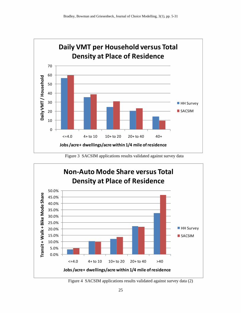
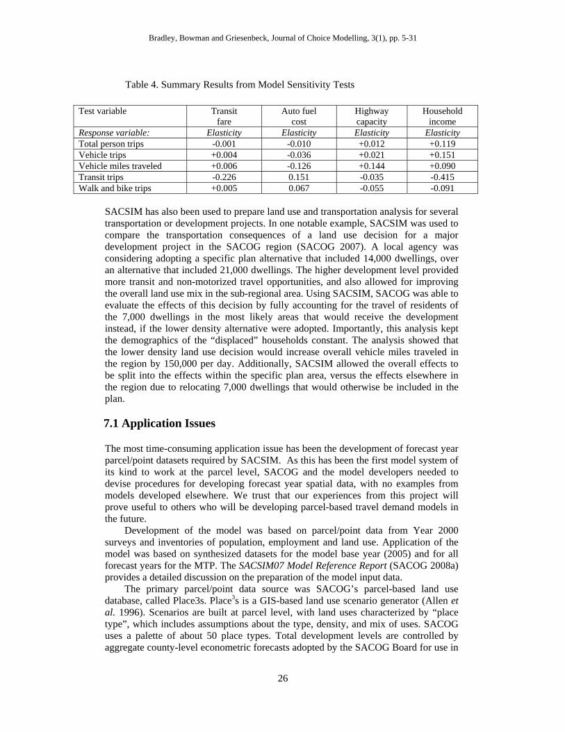
uses to traffic analysis zones. Figures 3 and 4 show how land use density (jobs plus dwelling units) within a quarter mile buffer around the residence parcel is related to daily VMT per household and non-auto mode share. The difference in behavior found in the survey households related to this density variable is quite dramatic, and the SACSIM predictions match the observed trends quite well. This ability to capture detailed neighborhood density effects is a result of the fact that the models use parcel-level detail, and that they use a variety of urban design variables.

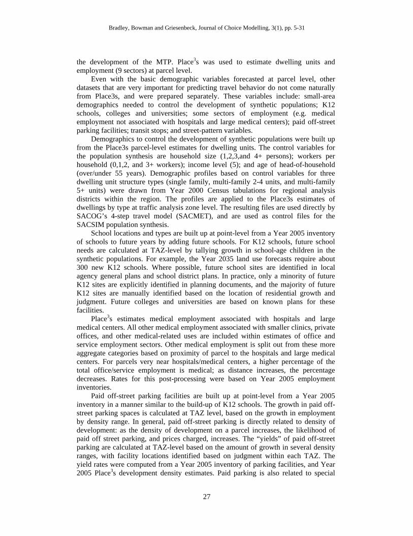
Travel sensitivities to transit fares, auto fuel cost, highway capacity, and household income were tested experimentally, by synthetically increasing or decreasing the test variable, and correlating changes in model outputs to the test variables. A summary of sensitivity test results is given in Table 4. For these tests, reasonability of the travel model sensitivity was judged by comparison to sensitivities observed in other research. For example, the transit fare elasticity is roughly -0.23, which is in the typical range. The cross-elasticities for the other modes and for total trips are quite low, due to the fact that the transit mode share is very low to begin with, so mode shifts from transit have little relative effect on the other modes.

The auto fuel cost elasticity on VMT is roughly -0.13. This is somewhat lower than the typical long term fuel price elasticity estimated from time series data (-0.2 to -0.3), and there is clearly a question as to how accurately cross-sectional data from a period of stable fuel prices can capture behavioral responses to fuel price. Also, the tests below were done for the 2005 situation, when there are few non-auto alternatives in several parts of the region. In additional scenarios run for 2035, with more compact land uses and increased transit service, the fuel price elasticity for the forecasts appears somewhat higher, around -0.018.

The estimated elasticity of VMT with regard to highway capacity (+0.144) also appears somewhat low, as time series analysis has revealed values in the range of +0.3 to +0.6. Note, however, that this sensitivity test was done not by adding new highway links, but simply by increasing the capacity on all existing road network links, regardless of the level of congestion. In real situations, roads tend to added and widened only where congestion levels are highest, so it is reasonable that the effect on demand would be higher. Further sensitivity tests could be done to more closely mimic real-world highway capacity improvements.

7 SACSIM Model Application

SACSIM was used to prepare forecasts and analysis of the most recent long range regional transportation plan, adopted in March 2007, for which SACSIM was used to forecast to Year 2035 (SACOG, 2008b). A unique aspect of the analysis prepared for the plan was a division of key travel metrics into “household-generated” travel, commercial vehicle travel and external travel. Because SACSIM accounts for all travel generated from households, including trips that in four-step models are lumped into “non-home-based” trips, a complete accounting of household-generated travel can be made. This analysis capability is extremely useful for transportation planning, because travel decisions away from the home are affected by characteristics of land uses at place of residence, as well as by travel choices made in earlier trips during the day.


0

10

20

30

40

50

60

70

<=4.0 4+ to 10 10+ to 20 20+ to 40 40+

Dai

ly V

MT

/ H

ouse

hold

Jobs /acre+ dwellings/acre within 1/4 mile of residence

Daily VMT per Household versus Total Density at Place of Residence

HH Survey

SACSIM

Figure 3 SACSIM applications results validated against survey data

0.0%

5.0%

10.0%

15.0%

20.0%

25.0%

30.0%

35.0%

40.0%

45.0%

50.0%

<=4.0 4+ to 10 10+ to 20 20+ to 40 >40

Tran

sit +

Wal

k +

Bike

Mod

e Sh

are

Jobs /acre+ dwellings/acre within 1/4 mile of residence

Non-Auto Mode Share versus Total Density at Place of Residence

HH Survey

SACSIM

Figure 4 SACSIM applications results validated against survey data (2)

25


26

Table 4. Summary Results from Model Sensitivity Tests

Test variable Transit fare

Auto fuel cost

Highway capacity

Household income

Response variable: Elasticity Elasticity Elasticity Elasticity Total person trips -0.001 -0.010 +0.012 +0.119 Vehicle trips +0.004 -0.036 +0.021 +0.151 Vehicle miles traveled +0.006 -0.126 +0.144 +0.090 Transit trips -0.226 0.151 -0.035 -0.415 Walk and bike trips +0.005 0.067 -0.055 -0.091

SACSIM has also been used to prepare land use and transportation analysis for several transportation or development projects. In one notable example, SACSIM was used to compare the transportation consequences of a land use decision for a major development project in the SACOG region (SACOG 2007). A local agency was considering adopting a specific plan alternative that included 14,000 dwellings, over an alternative that included 21,000 dwellings. The higher development level provided more transit and non-motorized travel opportunities, and also allowed for improving the overall land use mix in the sub-regional area. Using SACSIM, SACOG was able to evaluate the effects of this decision by fully accounting for the travel of residents of the 7,000 dwellings in the most likely areas that would receive the development instead, if the lower density alternative were adopted. Importantly, this analysis kept the demographics of the “displaced” households constant. The analysis showed that the lower density land use decision would increase overall vehicle miles traveled in the region by 150,000 per day. Additionally, SACSIM allowed the overall effects to be split into the effects within the specific plan area, versus the effects elsewhere in the region due to relocating 7,000 dwellings that would otherwise be included in the plan.

7.1 Application Issues

The most time-consuming application issue has been the development of forecast year parcel/point datasets required by SACSIM. As this has been the first model system of its kind to work at the parcel level, SACOG and the model developers needed to devise procedures for developing forecast year spatial data, with no examples from models developed elsewhere. We trust that our experiences from this project will prove useful to others who will be developing parcel-based travel demand models in the future.

Development of the model was based on parcel/point data from Year 2000 surveys and inventories of population, employment and land use. Application of the model was based on synthesized datasets for the model base year (2005) and for all forecast years for the MTP. The SACSIM07 Model Reference Report (SACOG 2008a) provides a detailed discussion on the preparation of the model input data.

The primary parcel/point data source was SACOG’s parcel-based land use database, called Place3s. Place3s is a GIS-based land use scenario generator (Allen et al. 1996). Scenarios are built at parcel level, with land uses characterized by “place type”, which includes assumptions about the type, density, and mix of uses. SACOG uses a palette of about 50 place types. Total development levels are controlled by aggregate county-level econometric forecasts adopted by the SACOG Board for use in


27

the development of the MTP. Place3s was used to estimate dwelling units and employment (9 sectors) at parcel level.

Even with the basic demographic variables forecasted at parcel level, other datasets that are very important for predicting travel behavior do not come naturally from Place3s, and were prepared separately. These variables include: small-area demographics needed to control the development of synthetic populations; K12 schools, colleges and universities; some sectors of employment (e.g. medical employment not associated with hospitals and large medical centers); paid off-street parking facilities; transit stops; and street-pattern variables.

Demographics to control the development of synthetic populations were built up from the Place3s parcel-level estimates for dwelling units. The control variables for the population synthesis are household size (1,2,3,and 4+ persons); workers per household (0,1,2, and 3+ workers); income level (5); and age of head-of-household (over/under 55 years). Demographic profiles based on control variables for three dwelling unit structure types (single family, multi-family 2-4 units, and multi-family 5+ units) were drawn from Year 2000 Census tabulations for regional analysis districts within the region. The profiles are applied to the Place3s estimates of dwellings by type at traffic analysis zone level. The resulting files are used directly by SACOG’s 4-step travel model (SACMET), and are used as control files for the SACSIM population synthesis.

School locations and types are built up at point-level from a Year 2005 inventory of schools to future years by adding future schools. For K12 schools, future school needs are calculated at TAZ-level by tallying growth in school-age children in the synthetic populations. For example, the Year 2035 land use forecasts require about 300 new K12 schools. Where possible, future school sites are identified in local agency general plans and school district plans. In practice, only a minority of future K12 sites are explicitly identified in planning documents, and the majority of future K12 sites are manually identified based on the location of residential growth and judgment. Future colleges and universities are based on known plans for these facilities.

Place3s estimates medical employment associated with hospitals and large medical centers. All other medical employment associated with smaller clinics, private offices, and other medical-related uses are included within estimates of office and service employment sectors. Other medical employment is split out from these more aggregate categories based on proximity of parcel to the hospitals and large medical centers. For parcels very near hospitals/medical centers, a higher percentage of the total office/service employment is medical; as distance increases, the percentage decreases. Rates for this post-processing were based on Year 2005 employment inventories.

Paid off-street parking facilities are built up at point-level from a Year 2005 inventory in a manner similar to the build-up of K12 schools. The growth in paid off-street parking spaces is calculated at TAZ level, based on the growth in employment by density range. In general, paid off-street parking is directly related to density of development: as the density of development on a parcel increases, the likelihood of paid off street parking, and prices charged, increases. The “yields” of paid off-street parking are calculated at TAZ-level based on the amount of growth in several density ranges, with facility locations identified based on judgment within each TAZ. The yield rates were computed from a Year 2005 inventory of parking facilities, and Year 2005 Place3s development density estimates. Paid parking is also related to special


28

uses, like colleges/universities and hospitals, and facilities are added at future locations of these uses.

Proximity to transit is measured as orthogonal distance from parcel to the nearest transit station or stop in SACSIM. Transit stops are also built up at point level from a Year 2005 inventory of transit stops. New future transit stop points are based on a comparison of forecast year and Year 2005 transit networks from the travel demand model. Where new transit lines are added, new stops are added to the inventory. In areas with little or no change in transit service, the Year 2005 stop inventory is used. For rail and express bus facilities, stations and stops as coded in the travel demand model are used directly. For fixed route bus services, the travel demand model stops under-predict actual stops. This is because zone-based travel models do not include sufficient detail to capture the stop-spacing for local bus routes, especially in urban areas. In these areas, stops points are synthesized along the bus routes and added to the Year 2005 inventory points.

Street pattern variables are used in several location and mode choice models in SACSIM, and are strongly related to non-motorized mode choice. The key street pattern variables are the buffered densities or numbers of intersections of three types: 1-leg intersections (e.g. cul-de-sacs); 3-leg intersections (e.g. a “T”); and 4+-leg intersections (e.g. a four-way intersection). Higher levels of 1-leg intersections are associated with lower likelihood of trip linking and non-motorized modes of travel; higher levels of 3- and 4+- leg intersections are associated with higher likelihood of trip linking and non-motorized travel modes. While future densities and mixes of use in growth areas are captured in the Place3s land use scenarios, future street pattern is not. Street patterns profiles for growth areas are “borrowed” from Year 2005 observed street patterns by place type and density level.

Each one of these data issues required significant time and effort to address. However, with the exception of transit stops, the data are prepared only once for each land use data run, and the process is becoming more routinized and efficient. Virtually all of these issues need to be addressed for zone-based models, but the aggregate nature of the zones allows for the data to be developed with less rigor and hand-wringing. The discipline of developing the datasets at parcel/point level simply requires that all the assumptions be laid out explicitly.

8 Peer Review Assessment and Recommendations

The SACSIM model system was the subject of a two-day peer review session, sponsored by the FHWA Travel Model Improvement Program (TMIP) in November 2008 (SACOG 2008c). All members of the peer review panel had experience with implementing activity-based models—four from the MPO perspective, and one from the model developer perspective.

In general, the review panelists were very positive about the SACSIM model system. The aspects of the activity-based model component (DaySim) that the review panel commended most highly were:

• The parcel-based approach • The tour-based approach (day-tour- trip hierarchy, time of day scheduling) • Treatment of university students throughout the model (UC-Davis and

Sacramento State Univ.), including a separate population synthesis for on-campus housing.

• The rigorous sensitivity testing performed


29

A variety of possible enhancements to the model system were also discussed. The specific improvements that the panel deemed highest priority were:

• Related to road pricing: o Update the value-of-time coefficients, and improve the treatment of

price (for example, a toll versus non-toll nest as part of mode choice) o Move to distributed values-of-time (a separate VOT for each

person/tour, drawn from distribution) • Related to destination choice:

o Change the specification of destination choice models to rely less on distance, and more on mode choice logsums and other mode level of service measures

• Related to mode choice: o Move toward adding additional pedestrian and bicycle supply

variables to the model (examples are sidewalk and bicycle lane coverage as a percentage of street distance within walking/biking distance around each parcel)

The last improvement mentioned above illustrates the type of additional detail that a parcel-level model can accommodate in order to allow analysis of urban design and non-motorized travel. It is likely that such urban infrastructure data will be readily available in digital form for most MPO’s in the near future.

9 Conclusions This article provides a detailed overview of the first parcel-based, activity-based travel demand model system to be used in urban forecasting, to the authors’ knowledge. The model system was used to provide the forecasts for the latest Regional Transportation Plan (RTP) for the Sacramento region, and a Federal peer review of the model system was carried out. We can conclude that it is possible to create and apply a regional demand model system using parcel-level geography and half-hour time of day periods. Experiences thus far have pointed to major benefits of using detailed land use variables and urban design variables, but also to new challenges in providing parcel-level land use inputs for future years. Further research is under way to integrate parcel-level travel demand microsimulation models with land use models such as PECAS (in the Sacramento region) and UrbanSim (in the Seattle region). In addition, Federal research projects are now underway to integrate the SACSIM model with dynamic traffic simulation models such as TRANSIMS and DYNUS-T, which can fully take advantage of the finer spatial and temporal detail in the travel demand forecasts, and can in turn provide DaySim with more accurate predictions of highway travel times and congestion.


30

References Abraham, J., Garry, G. and Hunt, J. D., 2004. The Sacramento PECAS Model.

Working paper. Available from [email protected]. Allen, E., McKeever, M. and Mitchum, J., 1996. The Energy Yardstick: Using Place3s

to Create More Sustainable Communities, California Energy Commission, the Oregon Department of Energy and the Washington State Energy Office. http://www.energy.ca.gov/places/.

Bhat, C. R., Guo, J. Y., Srinivasan, S. and Sivakumar, A., 2004. A Comprehensive Econometric Microsimulator for Daily Activity-Travel Patterns. Transportation Research Record 1894, 57-66,

Bowman, J. L., and Ben-Akiva, M., 2001. Activity-based disaggregate travel demand model system with activity schedules, Transportation Research Part A, 35(1), 1-28.

Bowman, J. L. and Bradley, M., 2005. Disaggregate Treatment of Purpose, Time of Day and Location in an Activity-Based Regional Travel Forecasting Model. Paper presented at the European Transport Conference, Strasbourg, France, October 3-5.

Bowman, J. L., Bradley, M. and Gibb, J., 2006. The Sacramento Activity-based Travel Demand Model: Estimation and Validation Results. Paper presented at the European Transport Conference, Strasbourg, France, September 18-20.

Bowman, J. L., and Bradley, M. A., 2006. Activity-Based Travel Forecasting Model for SACOG: Technical Memos Numbers 1-11. Available from http://jbowman.net.

Bradley, M., Bowman, J. L., Shiftan, Y., Lawton, T. K. and Ben-Akiva, M. E., 1998. A System of Activity-Based Models for Portland, Oregon. Report prepared for the Federal Highway Administration Travel Model Improvement Program. Washington, D.C.

Bradley, M., Bowman, J. L. and Lawton, T. K., 1999. A Comparison of Sample Enumeration and Stochastic Microsimulation for Application of Tour-Based and Activity-Based Travel Demand Models. Paper presented at European Transport Conference, Cambridge, UK, September 27-29.

Bradley, M. and Bowman, J., 2006. A summary of design features of activity-based microsimulation models for U.S. MPO’s. Conference on Innovations in Travel Demand Modeling, Austin, TX, http://trb.org/Conferences/TDM/papers/BS1A%20-%20Austin_paper_bradley.pdf

Bradley, M., Outwater, M., Jonnalagadda, N. and Ruiter, E., 2001. Estimation of an Activity-Based Micro-Simulation Model for San Francisco. Paper presented at the 80th Annual Meeting of the Transportation Research Board, Washington D.C.

Evans, S., 1976. Derivation and Analysis of Some Models Combining Trip Distribution and Assignment. Transportation Research Part B, 10(1), 37-57.

Jonnalagadda, N, J. Freedman, Davidson, W. and Hunt, J. D., 2001. Development of a Micro-Simulation Activity-based Model for San Francisco – Destination and Mode Choice Models. Transportation Research Record 1777, 25-35.

SACOG, 2007. Comments on Placer Vineyards Specific Plan: Second Revised Draft EIR. Sacramento Area Council of Governments, May.

SACOG, 2008a. Sacramento Activity-Based Travel Simulation Model (SACSIM07): Model Reference Report. Sacramento Area Council of Governments. November.

SACOG, 2008b. Sacramento Region 2035 Metropolitan Transportation Plan. Sacramento Area Council of Governments. http://sacog.org/mtp/2035/final-mtp/

SACOG, 2008c. SACSIM Improvement Program Peer Review Report. Sacramento Area Council of Governments, December.

mailto:[email protected]

http://www.energy.ca.gov/places/

http://jbowman.net/

http://trb.org/Conferences/TDM/papers/BS1A%20-%20Austin_paper_bradley.pdf

http://sacog.org/mtp/2035/final-mtp/


31

Vovsha, P. and Bradley, M., 2004. A Hybrid Discrete Choice Departure Time and Duration Model for Scheduling Travel Tours. Transportation Research Record 1894, 46-56.

Vovsha, P., Bradley, M. and Bowman, J. L., 2004. Activity-based travel forecasting models in the United States: Progress since 1995 and Prospects for the Future. Paper presented at the EIRASS Conference on Progress in Activity-Based Analysis, Maastricht, May 28-31.

Vovsha P., Petersen, E. and Donnelly, R., 2002. Micro-Simulation in Travel Demand Modeling: Lessons Learned from the New York Best Practice Model. Transportation Research Record 1805, 68-77.

Vovsha P., Petersen, E. and Donnelly, R., 2003 Explicit Modeling of Joint Travel by Household Members: Statistical Evidence and Applied Approach. Transportation Research Record 1831, 1-10.