4. Allgemeine Anregung - wandinger.userweb.mwn.dewandinger.userweb.mwn.de/LA_Elastodynamik_1/v2_4.pdf · Prof. Dr. Wandinger 2. Systeme mit 1 Freiheitsgrad Elastodynamik 1 2.4-12

Prof. Dr. Wandinger 2. Systeme mit 1 Freiheitsgrad Elastodynamik 12.4-1

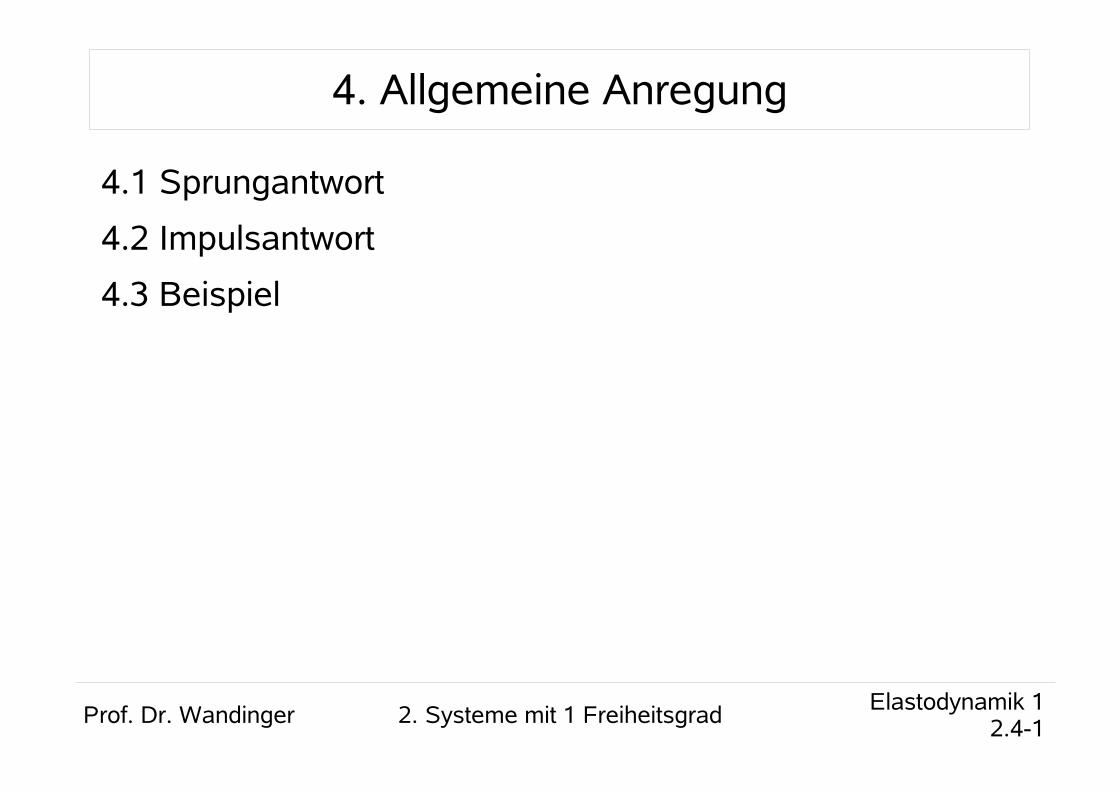
4. Allgemeine Anregung

4.1 Sprungantwort

4.2 Impulsantwort

4.3 Beispiel


4.1 Sprungantwort

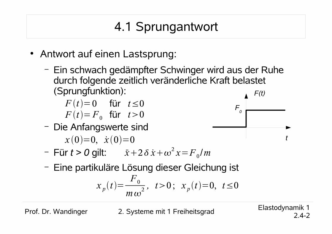
● Antwort auf einen Lastsprung:– Ein schwach gedämpfter Schwinger wird aus der Ruhe

durch folgende zeitlich veränderliche Kraft belastet (Sprungfunktion):

– Die Anfangswerte sind

– Für t > 0 gilt:– Eine partikuläre Lösung dieser Gleichung ist

F t =F t =

0F 0

fürfür

t≤0t0

x 0=0, x 0=0 t

F(t)

F0

x2 x2 x=F 0 /m

x p t =F 0m

2 , t0 ; x p t =0, t≤0


4.1 Sprungantwort

– Die allgemeine Lösung lautetmit (vgl. 2.1.3)

– Anfangsbedingungen:● :

● :

● Daraus:

x t =x pt x h t

x ht =e− t

C 1cos d t C 2sin d t

x 0=0 xh 0=−x p 0=−F 0m

2

x 0=0 x h 0=0

C1=xh 0=−F 0m

2

C 2=

d

x h 0=−

d

F 0m

2


4.1 Sprungantwort

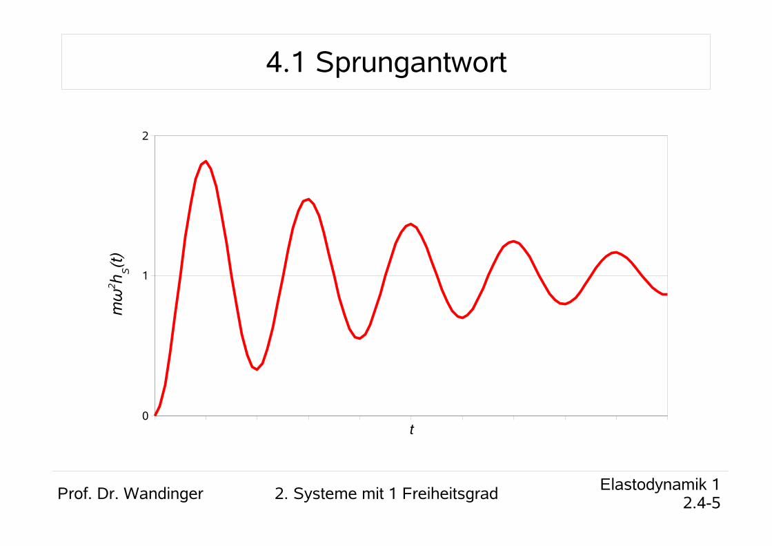
– Damit lautet die Lösung:

– Die Funktion

wird als Sprungantwort bezeichnet.– Mit der Sprungantwort gilt:

x t =F 0m

2 [1−e− t cosd t

d

sin d t ] , t0

hS t ={0, t≤01m

2 [1−e− t cosd t

d

sin d t ] , t0

x t =F 0hS t


0

1

2

t

mω

2 h S(t

)

4.1 Sprungantwort


4.1 Sprungantwort

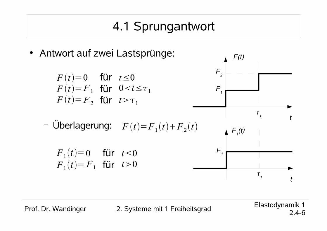
● Antwort auf zwei Lastsprünge:

– Überlagerung:

F t =F t =F t =

0F 1F 2

fürfürfür

t≤00t≤1

t1

t

F(t)

F1

F2

τ1

F t =F 1t F 2t

t

F1(t)

F1

τ1

F 1t =F 1t =

0F 1

fürfür

t≤0t0


4.1 Sprungantwort

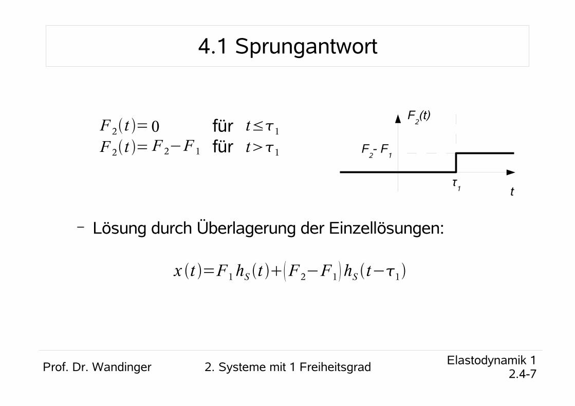
– Lösung durch Überlagerung der Einzellösungen:

F 2t =F 2t =

0F 2−F 1

fürfür

t≤1

t1

t

F2(t)

F2- F

1

τ1

x t =F1hS t F 2−F1 hS t−1


4.1 Sprungantwort

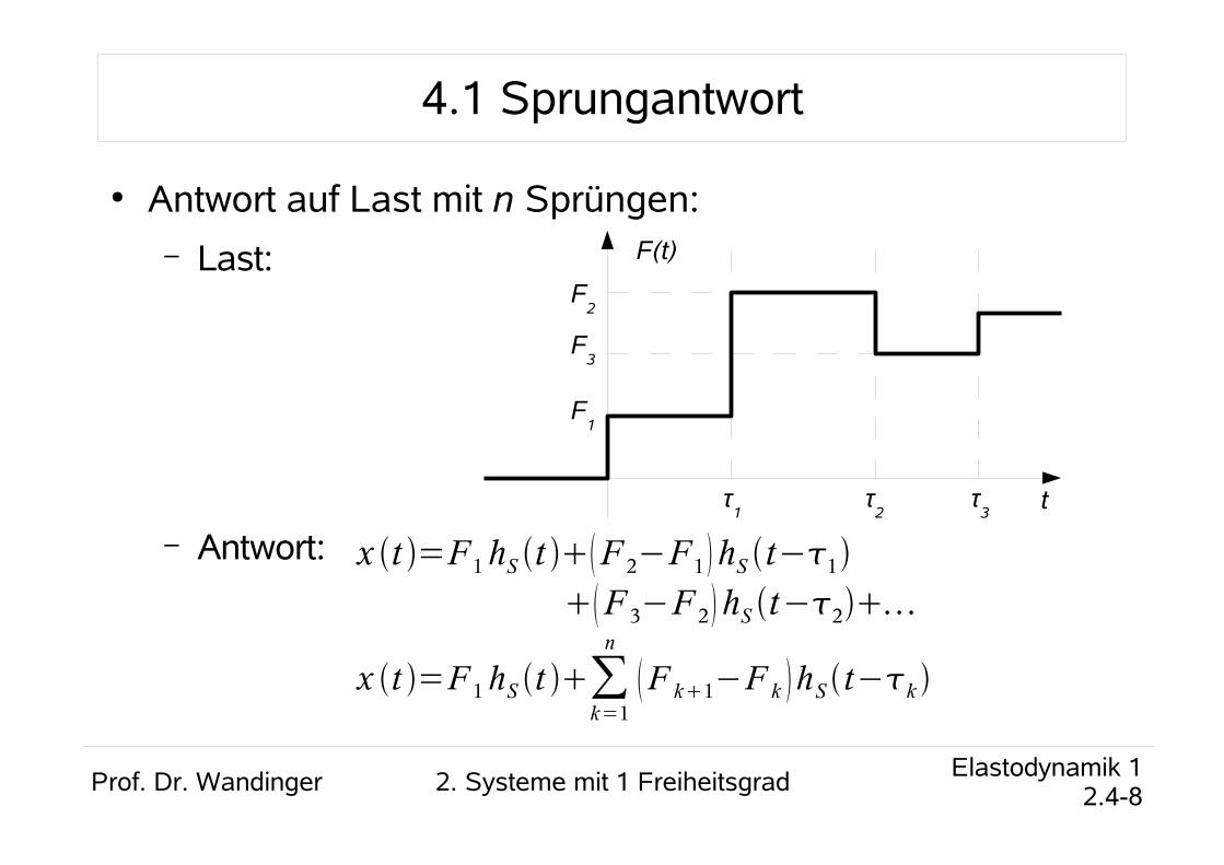
● Antwort auf Last mit n Sprüngen:– Last:

– Antwort:

t

F(t)

F1

F2

τ1

τ2

τ3

F3

x t =F1hS t F 2−F1 hS t−1

F 3−F 2 hS t−2

x t =F 1hS t ∑k=1

n

F k1−F k hS t−k


4.1 Sprungantwort

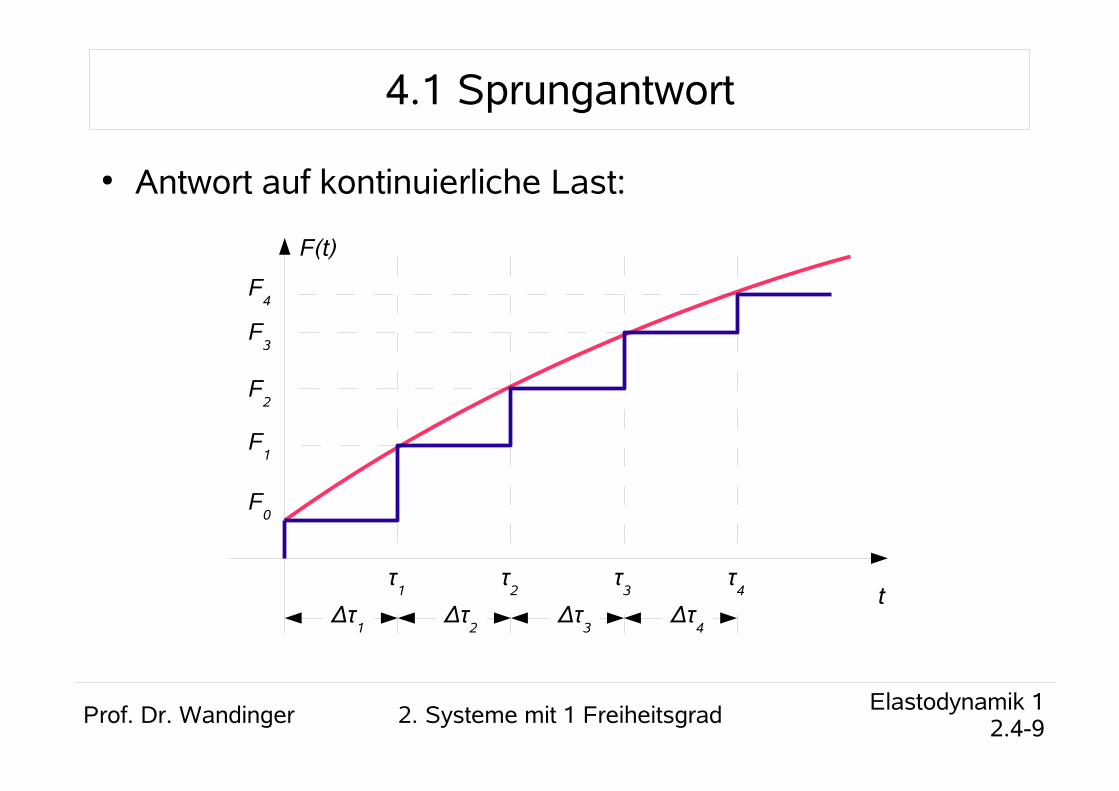
● Antwort auf kontinuierliche Last:

t

F(t)

τ1

τ2

τ3

τ4

F1

F2

F3

F4

F0

Δτ1

Δτ2

Δτ3

Δτ4


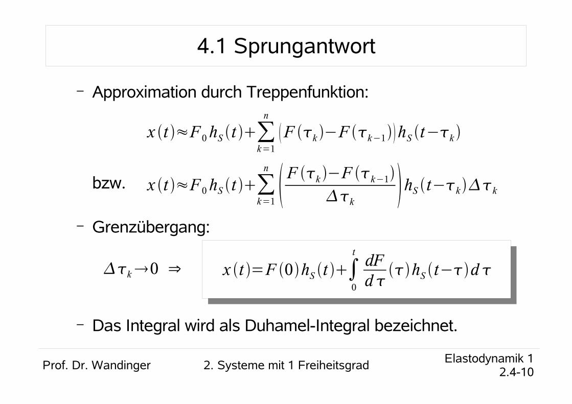
4.1 Sprungantwort

– Approximation durch Treppenfunktion:

bzw.

– Grenzübergang:

– Das Integral wird als Duhamel-Integral bezeichnet.

x t ≈F 0hS t ∑k=1

n

F k −F k−1hS t−k

x t ≈F 0hS t ∑k=1

n

F k −F k−1

k hS t−k k

k0 ⇒ x t =F 0hS t ∫0

tdFd

hS t−d


4.1 Sprungantwort

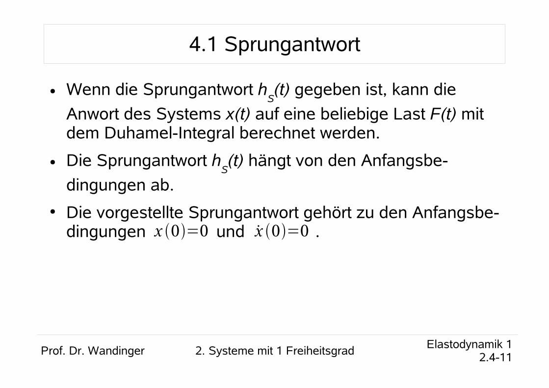
● Wenn die Sprungantwort hS(t) gegeben ist, kann die

Anwort des Systems x(t) auf eine beliebige Last F(t) mit dem Duhamel-Integral berechnet werden.

● Die Sprungantwort hS(t) hängt von den Anfangsbe-

dingungen ab.● Die vorgestellte Sprungantwort gehört zu den Anfangsbe-

dingungen und .x 0=0 x 0=0


4.2 Impulsantwort

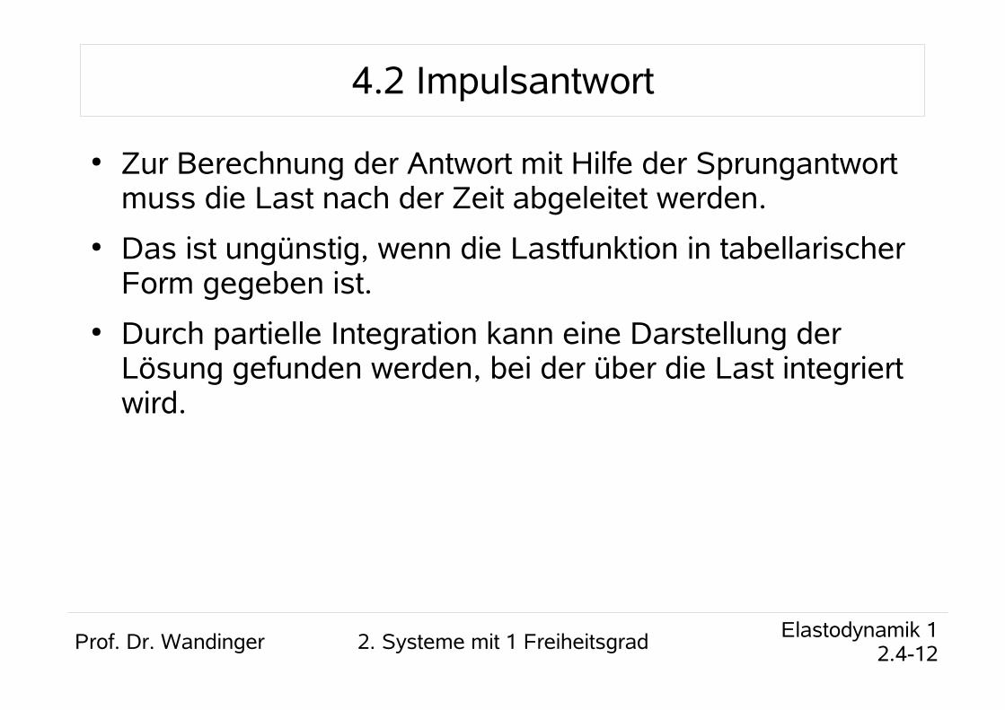
● Zur Berechnung der Antwort mit Hilfe der Sprungantwort muss die Last nach der Zeit abgeleitet werden.

● Das ist ungünstig, wenn die Lastfunktion in tabellarischer Form gegeben ist.

● Durch partielle Integration kann eine Darstellung der Lösung gefunden werden, bei der über die Last integriert wird.


4.2 Impulsantwort

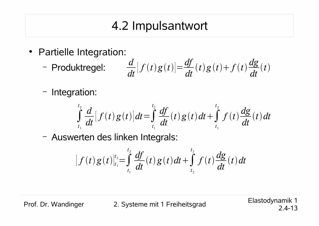
● Partielle Integration:– Produktregel:

– Integration:

– Auswerten des linken Integrals:

ddt

[ f t g t ]=dfdt

t g t f t dgdt

t

∫t1

t2ddt

[ f t g t ]dt=∫t1

t2dfdt

t g t dt∫t 1

t 2

f t dgdt

t dt

[ f t g t ]t 1t 2=∫

t1

t 2dfdt

t g t dt∫t2

t2

f t dgdt

t dt


4.2 Impulsantwort

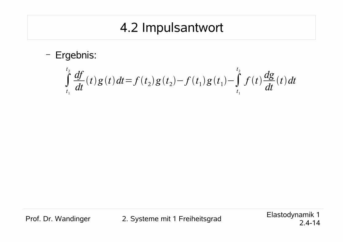
– Ergebnis:

∫t 1

t 2dfdt

t g t dt= f t2g t2− f t1g t1−∫t1

t2

f t dgdt

t dt


4.2 Impulsantwort

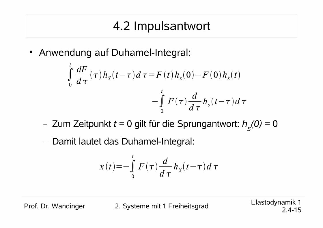
● Anwendung auf Duhamel-Integral:

– Zum Zeitpunkt t = 0 gilt für die Sprungantwort: hS(0) = 0

– Damit lautet das Duhamel-Integral:

∫0

tdFd

hS t−d =F t hs0−F 0hst

−∫0

t

F dd hs t−d

x t =−∫0

t

F dd hS t−d


4.2 Impulsantwort

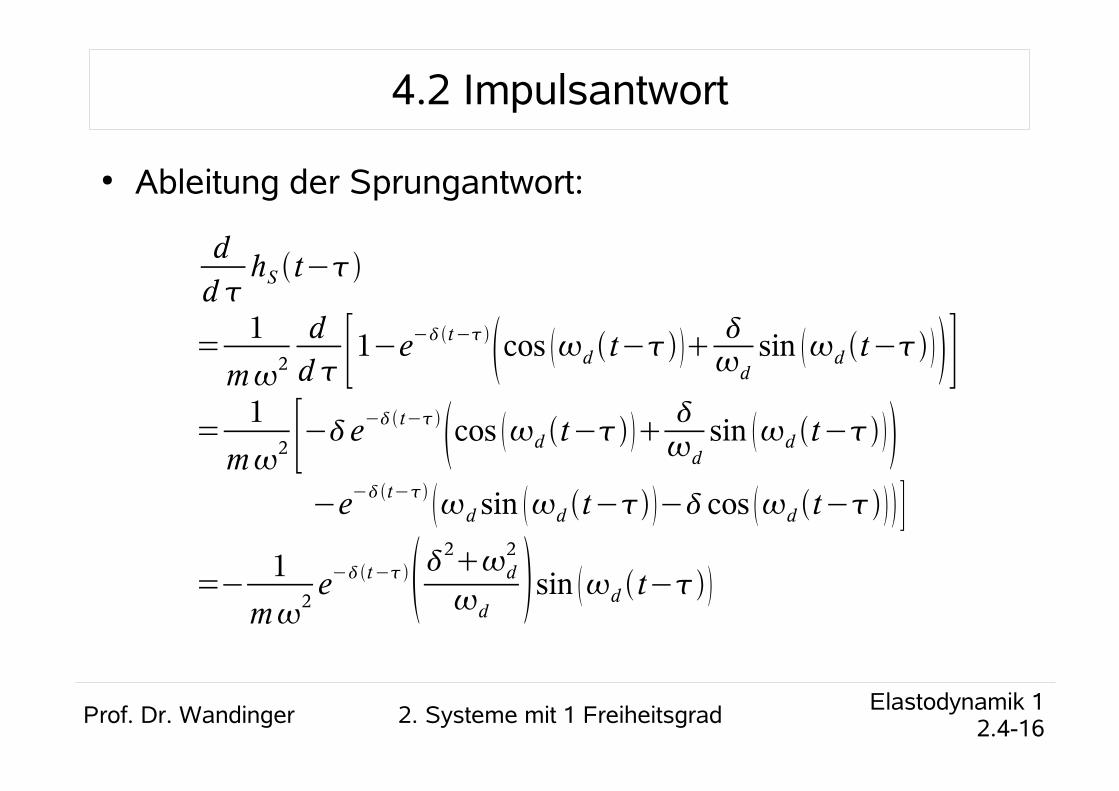
● Ableitung der Sprungantwort:

dd hS t−

=1

m2

dd [1−e

−t−

cos d t−

dsin d t− ]

=1

m2 [−e− t−

cos d t−

dsin d t−

−e−t−

d sin d t− − cos d t− ]

=−1

m2e−t−

2d

2

dsin d t−


4.2 Impulsantwort

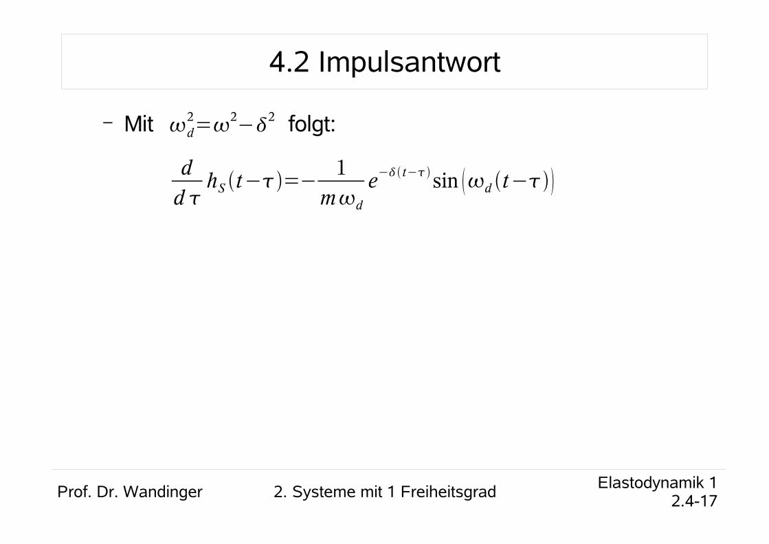
– Mit folgt:d2=

2−

2

dd hS t−=−

1md

e− t−sin d t−


4.2 Impulsantwort

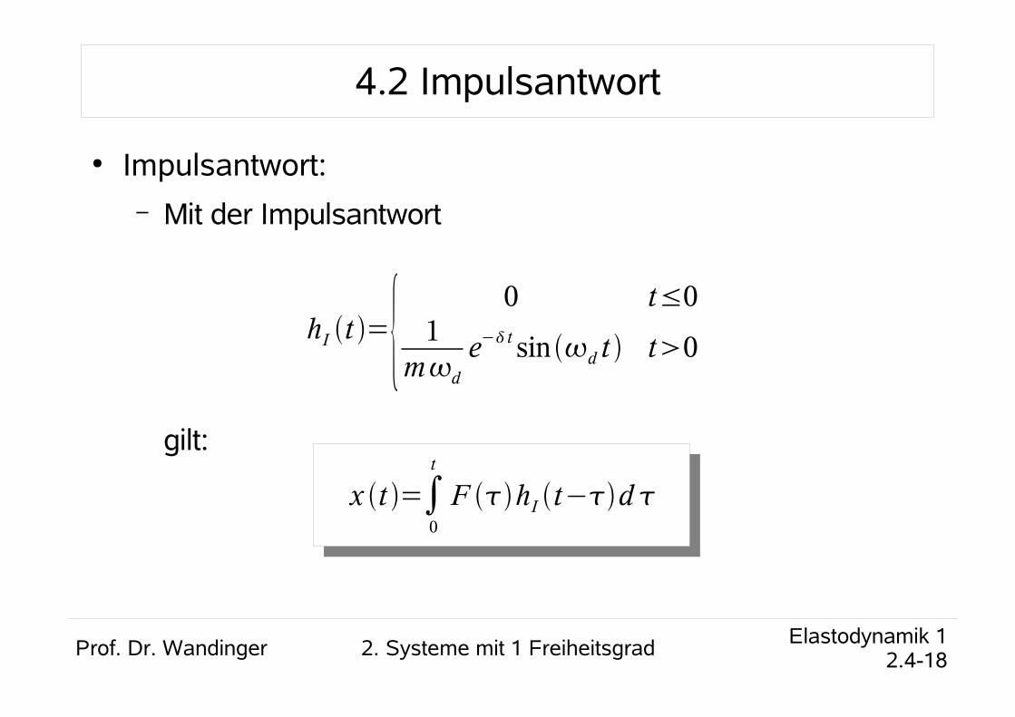
● Impulsantwort:– Mit der Impulsantwort

gilt:

hI t ={0 t≤0

1md

e− t sin d t t0

x t =∫0

t

F hI t−d


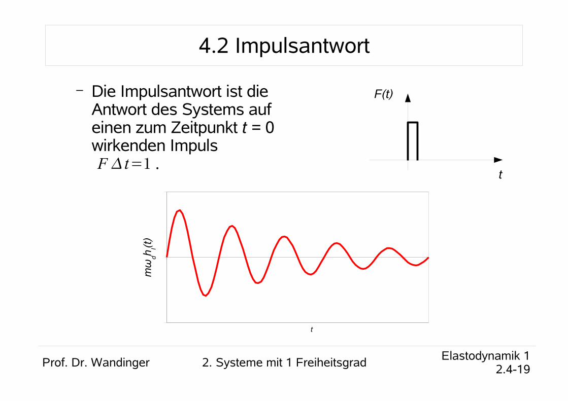
4.2 Impulsantwort

– Die Impulsantwort ist die Antwort des Systems auf einen zum Zeitpunkt t = 0 wirkenden Impuls .

t

F(t)

F t=1

t

mω

dh I(t)


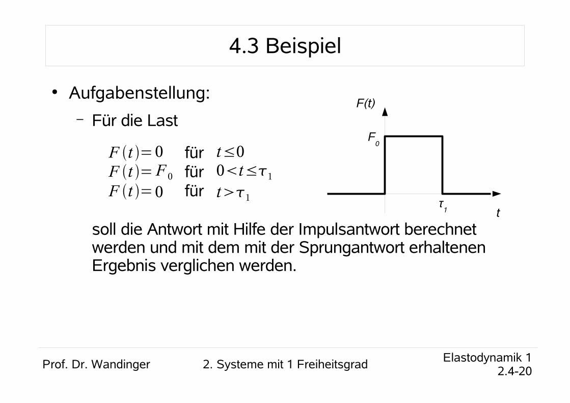
4.3 Beispiel

● Aufgabenstellung:– Für die Last

soll die Antwort mit Hilfe der Impulsantwort berechnet werden und mit dem mit der Sprungantwort erhaltenen Ergebnis verglichen werden.

F t =F t =F t =

0F 00

fürfürfür

t≤00t≤1

t1t

F(t)

F0

τ1


4.3 Beispiel

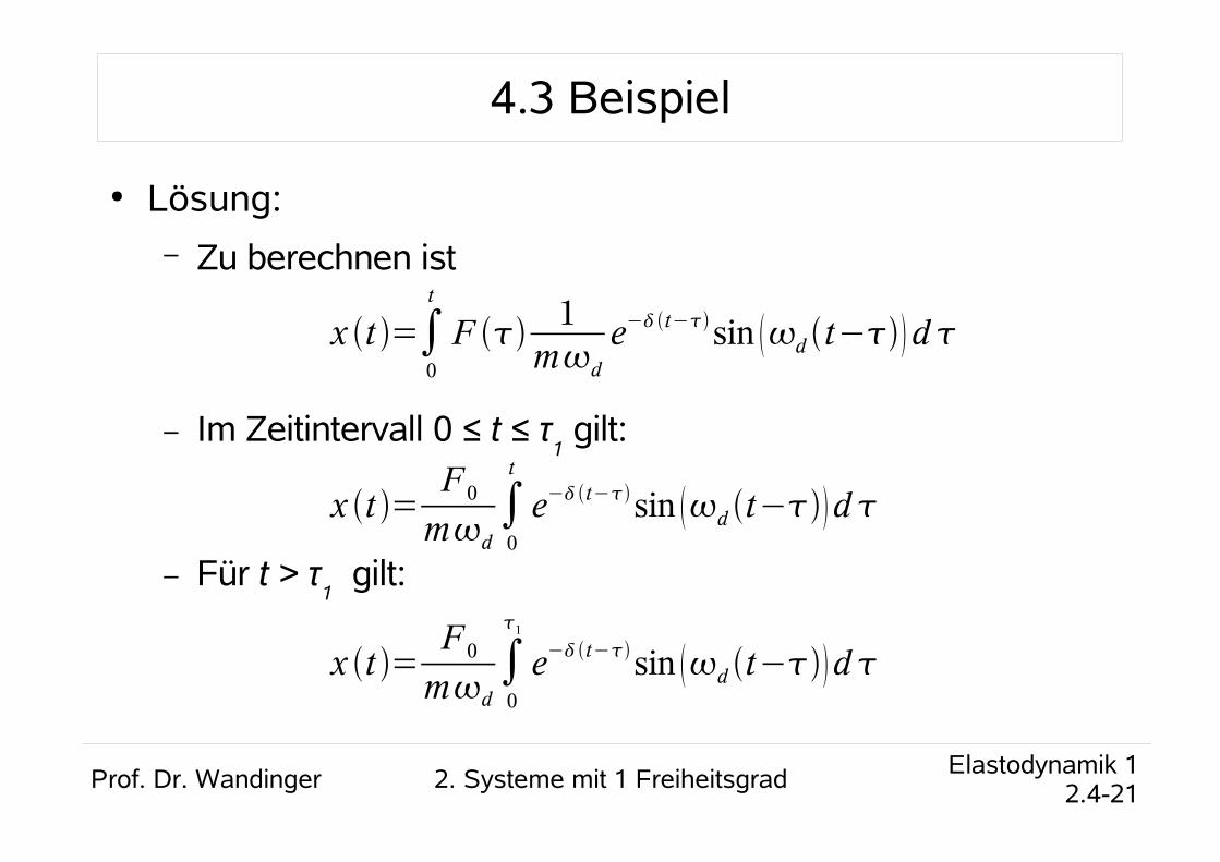
● Lösung:– Zu berechnen ist

– Im Zeitintervall 0 ≤ t ≤ τ1 gilt:

– Für t > τ1 gilt:

x t =∫0

t

F 1md

e−t−sin d t−d

x t =F 0md

∫0

t

e−t−sin d t−d

x t =F 0md

∫0

1

e−t−sin d t−d


4.3 Beispiel

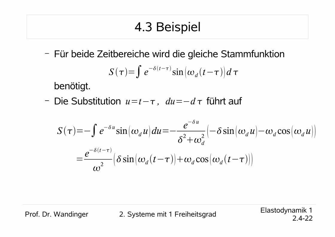
– Für beide Zeitbereiche wird die gleiche Stammfunktion

benötigt.– Die Substitution führt auf

S =∫ e− t−sin d t− d

u=t− , du=−d

S =−∫e−usin d u du=−

e−u

2d

2 −sin d u −d cos d u

=e−t−

2 sin d t−d cos d t−


4.3 Beispiel

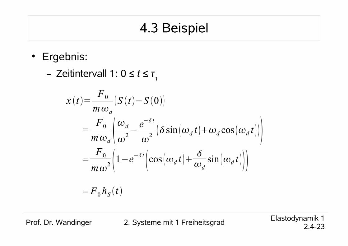
● Ergebnis:

– Zeitintervall 1: 0 ≤ t ≤ τ1

x t =F 0md

S t −S 0

=F 0md

d

2−e− t

2 sin d t d cos d t

=F 0

m2 1−e

− t

cos d t

dsin d t

=F 0hS t


4.3 Beispiel

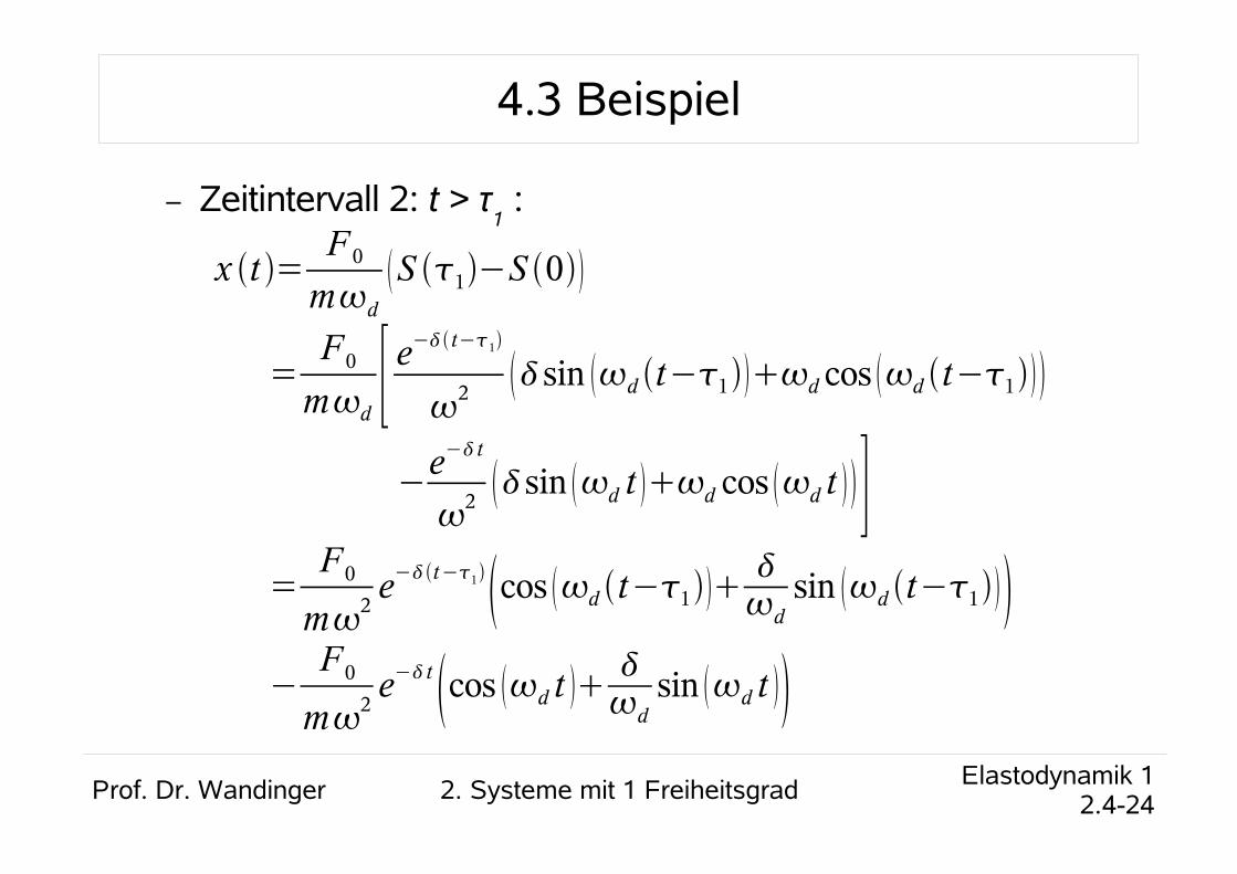
– Zeitintervall 2: t > τ1 :

x t =F 0md

S 1−S 0

=F0md

[ e− t−1

2 sin d t−1d cos d t−1

−e− t

2 sin d t d cos d t ]

=F0m

2e−t−1cos d t−1

dsin d t−1

−F0m

2e− t

cos d t

dsin d t


4.3 Beispiel

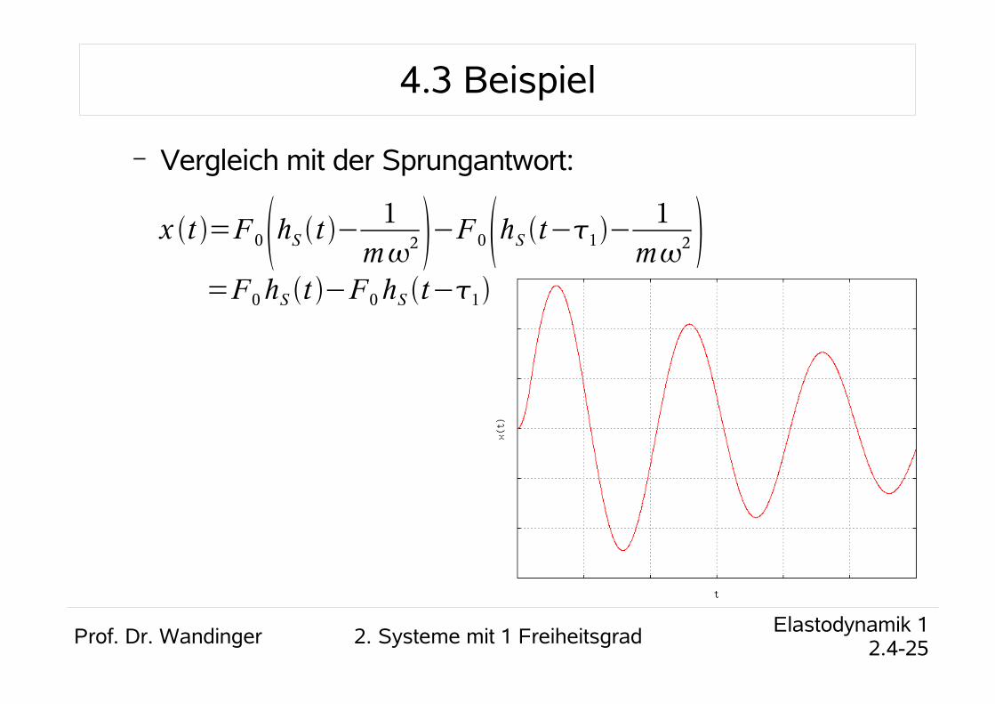
– Vergleich mit der Sprungantwort:

x t =F 0hS t −1m

2 −F 0hS t−1−1m

2 =F0hS t −F0hS t−1

Documents

4. Allgemeine Anregung - wandinger.userweb.mwn.dewandinger.userweb.mwn.de/LA_Elastodynamik_1/v2_4.pdf · Prof. Dr. Wandinger 2. Systeme mit 1 Freiheitsgrad Elastodynamik 1 2.4-12