Bayesian inference of non-linear multiscale model parameters

accelerated by a Deep Neural Network

Ling Wua,∗, Kepa Zulueta Uriondob, Zoltan Majorc, Aitor Arriagab, Ludovic Noelsa

aUniversity of Liege, CM3, Allee de la decouverte 9, B-4000 Liege, BelgiumbLeartiker Polymer R&D, Xemein Etorbidea 12A, 48270 Markina-Xemein, Bizkaia, Spain

cJohannes Kepler University Linz, Institute of Polymer Product Engineering, Altenbergerstrasse 69, 4040Linz, Austria

Abstract

We develop a Bayesian Inference (BI) of a non-linear multiscale model and material pa-

rameters using experimental composite coupons tests as observation data. In particular

we consider non-aligned Short Fibers Reinforced Polymer (SFRP) as a composite material

system and Mean-Field Homogenization (MFH) as a multiscale model. Although MFH is

computationally efficient, when considering non-aligned inclusions, the evaluation cost of a

non-linear response for a given set of model and material parameters remains too prohibitive

to be coupled with the sampling process required by the BI. Therefore, a Neural-Network-

type (NNW) is first trained using the MFH model, and is then used as a surrogate model

during the BI process, making the identification process affordable.

Keywords: Multiscale, Composites, Bayesian inference, Neural Network, Non-linear

1. Introduction

Short Fibers Reinforced Polymer (SFRP) composites are nowadays commonly used in

several industrial applications, increasing the need for computationally efficient modeling

tools. Because of the heterogeneous nature of the material, multiscale methods are favored

[1], in particular in the non-linear range, in order to capture the effects of the micro-structure

∗Corresponding author: L.Wu@ulg.ac.beEmail address: Zoltan.Major@jku.at (Zoltan Major)

Preprint submitted to Elsevier October 9, 2019

geometrical parameters, such as the inclusions aspect ratio, orientation and spatial distri-

butions, and of the micro-constituents non-linear material responses.

Mean-Field Homogenization (MFH) is an efficient semi-analytical multiscale method

which extends the Eshelby single inclusion solution [2] to multiple-inclusion interactions,

such as in the Mori-Tanaka (M-T) scheme [3]. In the non-linear range, MFH revolves

around the definition of a Linear Comparison Composite (LCC) [4–6] as a virtual hetero-

geneous linear material system, allowing to extend linear theories while keeping a good to

excellent accuracy. Two-step MFH has also been developed in the context of non-aligned

inclusions using an orientation distribution function (ODF) to describe their misalignment.

Homogenization is thus performed in two stages, first on pseudo-grains of aligned inclusions,

and then by weighting the pseudo-grain responses with the ODF [7, 8]. Since the manu-

facturing process induces a variation of the ODF along the sample thickness, this 2-step

homogenization has to be repeated on different layers to account for the so-called skin-core

effect.

One of the difficulty with multiscale methods in general, and MFH in particular, is to

identify the parameters defining the microstructure such as fibers aspect ratio distribution,

volume fraction, ODF, but also the material laws parameters modeling the phases non-linear

responses. On the one hand, fibers ODF, or again volume fraction can be experimentally

measured [9] or predicted by a process numerical simulation [9]. However, although the

fiber aspect ratio distribution can be experimentally measured, when using the ODF in the

context of a two-step MFH, it is convenient to consider a unique “effective” aspect ratio,

which has yet to be identified. On the other hand, although fibers properties of SFRP

are usually known, the matrix material properties is sensitive to the process conditions

and cannot always be directly identified because of the difficulty to produce samples whose

material response is exactly the same as the polymeric matrix of the composite material; the

parameters of the polymeric material models are thus generally obtained through an inverse

identification process from composite coupons tests.

Therefore some micro-structure geometrical parameters, such as the effective aspect ra-

tio, and some phases material parameters, such as the matrix model parameters, should be

2

inferred from composite experimental responses. However, because of the number of param-

eters arising in the non-linear range, this identification requires several loading conditions to

be performed, and a unique set of parameters cannot reproduce all the experimental tests

because of the model limitations. Besides, the composite responses are inevitably entailed

by experimental errors. These difficulties can be circumvented by considering a Bayesian

Inference (BI) [10] for which uncertainties in the inferred model parameters arise from the

identification process itself under the form of a so-called posterior Probability Density Func-

tion (PDF). This posterior PDF of the parameters set is the correction of the initial belief

one has on the parameters set distribution, or prior distribution, by a likelihood function

evaluated using different observation data, i.e. here the experimental results.

BI was extensively applied to identify the parameters of either, possibly non-linear, homo-

geneous material models [11–13, e.g.] or, generally linear, homogenized composite material

models [14, 15, e.g ]. The inference of multi-scale model parameters is more difficult because

of its inherent computational cost making the evaluation of the likelihood time consuming

when considering a random sampling process. Although in [16] the authors have inferred

the two-step MFH parameters of SFRP, this was limited to the linear range because of the

computational cost bottleneck: when considering a two-step homogenization as a non-linear

multiscale model, one simple analysis needs around one minute of computation but hundreds

of thousands of simulations are required for the sampling process. In order to make BI com-

putationally affordable in the non-linear range, in this work, the two-step MFH model is

substituted by a surrogate model during the random sampling process. The surrogate model

can be any kind of feasible high dimensional nonlinear mapping. Depending on the features

of the input and output, typical surrogate models can be constructed by linear combinations

of well chosen high dimensional nonlinear base functions. However, a certain experience is

required to choose the proper dimension of the function base and the order of the nonlinear

functions. Neural Networks (NNW) can theoretical carry out any high dimensional non-

linear mapping if the NNW is designed with enough hidden layers and enough neurons on

them. With the help of open NNW library, the experience required to build a high dimen-

sional nonlinear surrogate model is minimized, which offers a more user-friendly and general

3

solution. Artificial Neural Networks (ANNW) have been used in the literature to reproduce

the homogenized behavior predicted by computational homogenization methods, either by

approximating the strain energy density surface [17, 18, e.g.] or the stress-strain responses

[19, 20, e.g.]. The latter approach is chosen in the paper, and a NNW is trained by the two-

step MFH for different sets of micro-structure geometrical and material parameters, and

for different loading directions. The likelihood function is then constructed by considering

Gaussian noise [11–13] as an error function [15] evaluated from the experimental observation

on 40% of weight GF reinforced PA06 (PA06-GF40) coupon tests. The BI is then conducted

using a Metropolis-Hastings (MCMC) random walk during which the likelihood is evaluated

using the NNW as surrogate.

The organization of the paper is as follows. The non-linear two-step MFH model is

described in Section 2. Section 3 details the construction of the NNW surrogate model and

Section 4 summarizes the experimental tests conducted on PA06-GF40 composite coupons.

Finally, the BI is presented in Section 5 and the results analysis in Section 6. Conclusions

are drawn in Section 7.

2. Mean-field homogenization for non-aligned short fiber-reinforced composites

The finite element analysis of structures made of heterogeneous materials can be per-

formed in a homogenization-based multiscale approach, in which the relation between the

macro-strains εM and stresses σM is transformed into a relation between the averaged values

of the local strain tensor εm and of the local stress tensor σm on a micro-scale volume ω,

with

εM = 〈εm〉ω and σM = 〈σm〉ω , (1)

where 〈f(xxx)〉ω = 1Vω

∫ωf(x)dV , with Vω the volume of ω.

With a view to the homogenization of SFRP composites, the general equations for two-

phase composites with aligned uniform inclusions are first presented, the two-step homog-

enization method for non-aligned inclusions is then summarized before being extended to

account for skin-core effect. Finally the material models used for the different phases are

4

summarized.

2.1. Mean-Field Homogenization (MFH) for two-phase composites

2.1.1. Mean-field equations for two-phase linear elastic materials

Considering a two-phase composite material with the respective volume fractions v0+vI =

1, where the subscript 0 refers to the matrix and the subscript I to the aligned inclusions,

the volume averages over the micro-scale volume ω, Eqs. (1), can be explicitly expressed in

terms of the volume averages over the two phases ω0 and ωI, as

εM = v0ε0 + vIεI and σM = v0σ0 + vIσI , (2)

where •i denotes the volume average over the phase ωi, i.e. 〈•m〉ωi , for conciseness.

In the linear elastic range, the system of Eqs. (2) is completed by assuming a relationship

between the average strains of the different phases using a strain concentration tensor Bε,

which is defined through the elastic tensors Celi in phase ωi, and reads

εI = Bε(I,Cel0 , Cel

I ) : ε0 , (3)

where “I” represents the geometry of the inclusions. Using linear elastic constitutive laws

σi = Celi : εi, the set of Eqs. (2) and (3) can be rewritten in a general constitutive expression

for linear elastic composites as

σM = CelM(I,Cel

0 ,CelI , vI) : εM , (4)

with CelM =

[vICel

I : Bε(I,Cel0 , Cel

I ) + v0Cel0

]:[vIBε(I,Cel

0 , CelI ) + v0I

]−1, where (I)ijkl is the

identity fourth-order tensor.

2.1.2. Mean-field equations for two-phase elasto-plastic materials

For the composites whose phases experience elasto-plastic deformations, MFH is carried

out in an incremental form through a so-called Linear Comparison Composite (LCC) [21, 22].

The LCC is a virtual linear heterogeneous material whose constituents behaviors are defined

by virtual elastic operators matching the linearized behaviors of the real composite material

5

∆𝜀Munload

𝜀M

𝜎M 𝜎M𝑛

𝜎M𝑛+1

∆𝜀Mr

ℂMS

ℂMel

𝜀M 𝑛res

(a) Composite

∆𝜀𝑖unload

𝜀𝑖

𝜎𝑖 𝜎𝑖𝑛

𝜎𝑖𝑛+1

∆𝜀𝑖r

ℂ𝑖S

ℂ𝑖el

𝜀𝑖 𝑛res

𝜎𝑖 𝑛res

(b) Phase ωi

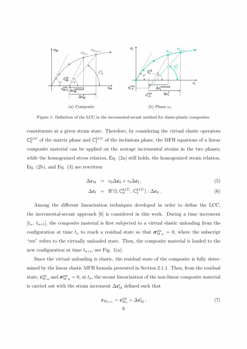
Figure 1: Definition of the LCC in the incremental-secant method for elasto-plastic composites.

constituents at a given strain state. Therefore, by considering the virtual elastic operators

CLCC0 of the matrix phase and CLCC

I of the inclusions phase, the MFH equations of a linear

composite material can be applied on the average incremental strains in the two phases;

while the homogenized stress relation, Eq. (2a) still holds, the homogenized strain relation,

Eq. (2b), and Eq. (3) are rewritten

∆εM = v0∆ε0 + vI∆εI , (5)

∆εI = Bε(I,CLCC0 , CLCC

I ) : ∆ε0 . (6)

Among the different linearization techniques developed in order to define the LCC,

the incremental-secant approach [6] is considered in this work. During a time increment

[tn, tn+1], the composite material is first subjected to a virtual elastic unloading from the

configuration at time tn to reach a residual state so that σresM n = 0, where the subscript

“res” refers to the virtually unloaded state. Then, the composite material is loaded to the

new configuration at time tn+1, see Fig. 1(a).

Since the virtual unloading is elastic, the residual state of the composite is fully deter-

mined by the linear elastic MFH formula presented in Section 2.1.1. Then, from the residual

state, εresM n and σres

M n = 0, at tn, the secant linearization of the non-linear composite material

is carried out with the strain increment ∆εrM defined such that

εMn+1 = εresMn

+ ∆εrM , (7)

6

where εMn+1 is a known value of at the macro-scale. Similarly, the phase strain increments

∆εri are defined such that

εin+1 = εresin + ∆εr

i , (8)

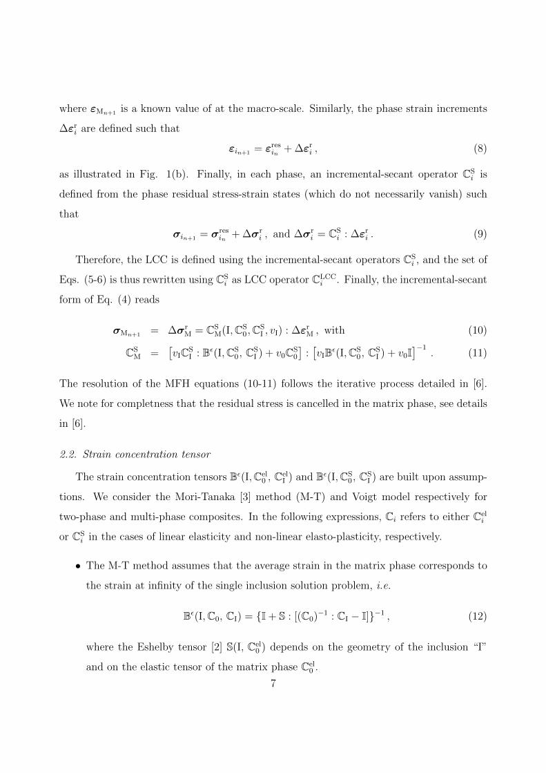
as illustrated in Fig. 1(b). Finally, in each phase, an incremental-secant operator CSi is

defined from the phase residual stress-strain states (which do not necessarily vanish) such

that

σin+1 = σresin + ∆σr

i , and ∆σri = CS

i : ∆εri . (9)

Therefore, the LCC is defined using the incremental-secant operators CSi , and the set of

Eqs. (5-6) is thus rewritten using CSi as LCC operator CLCC

i . Finally, the incremental-secant

form of Eq. (4) reads

σMn+1 = ∆σrM = CS

M(I,CS0,CS

I , vI) : ∆εrM , with (10)

CSM =

[vICS

I : Bε(I,CS0, CS

I ) + v0CS0

]:[vIBε(I,CS

0, CSI ) + v0I

]−1. (11)

The resolution of the MFH equations (10-11) follows the iterative process detailed in [6].

We note for completness that the residual stress is cancelled in the matrix phase, see details

in [6].

2.2. Strain concentration tensor

The strain concentration tensors Bε(I,Cel0 , Cel

I ) and Bε(I,CS0, CS

I ) are built upon assump-

tions. We consider the Mori-Tanaka [3] method (M-T) and Voigt model respectively for

two-phase and multi-phase composites. In the following expressions, Ci refers to either Celi

or CSi in the cases of linear elasticity and non-linear elasto-plasticity, respectively.

• The M-T method assumes that the average strain in the matrix phase corresponds to

the strain at infinity of the single inclusion solution problem, i.e.

Bε(I,C0, CI) = {I + S : [(C0)−1 : CI − I]}−1 , (12)

where the Eshelby tensor [2] S(I, Cel0 ) depends on the geometry of the inclusion “I”

and on the elastic tensor of the matrix phase Cel0 .

7

• The Voigt model assumes the same average strain in the different phases, i.e.

Bε = I . (13)

2.3. MFH for multi-phase composite materials

For short-fiber reinforced composites, the composite material cannot be treated as be-

ing two-phase in the MFH process because of the misalignment and of the variation in

aspect ratio of the fibers. When considering such a material with inclusions having different

orientations or shapes, a two-step homogenization strategy [7, 8] can be adopted.

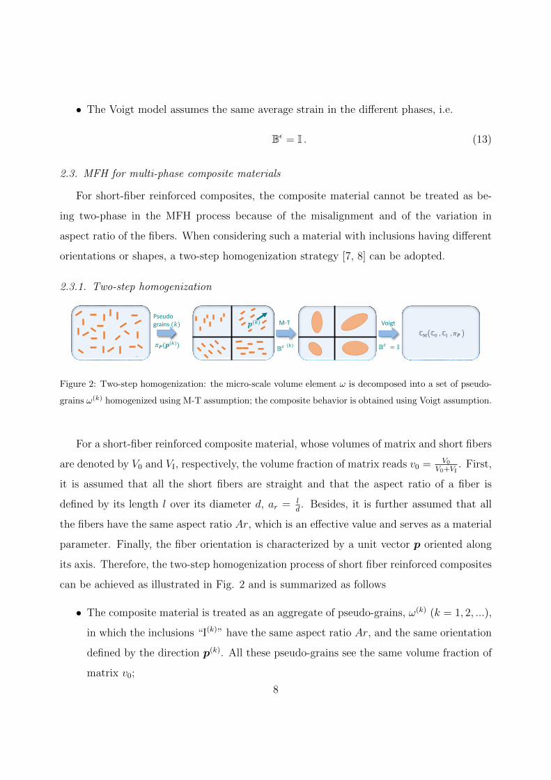
2.3.1. Two-step homogenization

Pseudo grains (𝑘)

𝜋𝑷(𝒑(𝑘))

M-T

𝔹𝜀 (𝑘)

Voigt

𝔹𝜀 = 𝕀

ℂM ℂ0 , ℂI , 𝜋𝑷

𝒑(𝑘)

Figure 2: Two-step homogenization: the micro-scale volume element ω is decomposed into a set of pseudo-

grains ω(k) homogenized using M-T assumption; the composite behavior is obtained using Voigt assumption.

For a short-fiber reinforced composite material, whose volumes of matrix and short fibers

are denoted by V0 and VI, respectively, the volume fraction of matrix reads v0 = V0

V0+VI. First,

it is assumed that all the short fibers are straight and that the aspect ratio of a fiber is

defined by its length l over its diameter d, ar = ld. Besides, it is further assumed that all

the fibers have the same aspect ratio Ar, which is an effective value and serves as a material

parameter. Finally, the fiber orientation is characterized by a unit vector p oriented along

its axis. Therefore, the two-step homogenization process of short fiber reinforced composites

can be achieved as illustrated in Fig. 2 and is summarized as follows

• The composite material is treated as an aggregate of pseudo-grains, ω(k) (k = 1, 2, ...),

in which the inclusions “I(k)” have the same aspect ratio Ar, and the same orientation

defined by the direction p(k). All these pseudo-grains see the same volume fraction of

matrix v0;

8

• The homogenization is first performed on each pseudo-grain ω(k), with the set of Eqs.

(5-6) rewritten as

〈∆ε〉ω(k) = v0〈∆ε0〉ω(k) + vI〈∆εI〉ω(k) , (14)

〈σ〉ω(k) = v0〈σ0〉ω(k) + vI〈σI〉ω(k) , (15)

〈∆εI〉ω(k) = Bε(

I(k), CS0, CS

I

): 〈∆ε0〉ω(k) . (16)

• The homogenization on the aggregate of pseudo-grains, ω(k) (k = 1, 2, ...) is then

achieved using Voigt strain concentration tensor (13), in which case the set of Eqs.

(5-6) is rewritten as

〈∆ε〉ω(k) = 〈∆ε〉ω = ∆εM ∀ω(k) , (17)

with the homogenized stress evaluated by

σM = 〈σ〉ω =∑k

vω(k)〈σ〉ω(k) , (18)

where vω(k) is the volume fraction defined by the volume of fibers having an oriented

along a direction p(k), Vω(k) , over the total volume of fibers VI, e.g. vω(k) =Vω(k)

VI. The

values of vω(k) can be approximated using a fibers Orientation Distribution Function.

2.3.2. Orientation Distribution Function (ODF)

For a collection of fibers, the complete description of their orientations is represented by

a probability density function πP (p), also called Orientation Distribution Function (ODF),

such that πP (p) dp is the probability of a fiber to be oriented between p and p + dp with∮πP (p) dp=1. It is convenient to write the ODF in the spherical coordinates as∫ π

θ=0

∮ 2π

φ=0

πP (p(θ, φ)) sin(θ) dφ dθ = 1 , (19)

where θ is the polar angle and φ is the azimuthal angle. In practice, the ODF πP (p) is not

always directly available, and it is commonly constructed through a second-order orientation

tensor, which reads [8, 23],

a =

∮p⊗ pπP (p) dp . (20)

9

More details on the construction of πP (p(θ, φ)) from a can be found in [8, 16]. Since a

constant fiber aspect ratio Ar is assumed, the value of vω(k) , in Eq. (18), can be approximated

by the volume fraction of fibers whose orientations are within [p(k)− 12∆p , p(k)+ 1

2∆p]. Using

the expression of ODF in the spherical coordinates, Eq. (19), we have

vω(k) ≈∫ θ(k)+ ∆θ

2

θ(k)−∆θ2

∮ φ(k)+ ∆φ2

φ(k)−∆φ2

πP (p(θ, φ)) sin(θ) dφ dθ , (21)

where θ(k) and φ(k) are respectively the polar and azimuthal angles of orientation p(k). The

angle increments ∆θ = π/Nπ2, and ∆φ = π/Nθ with Nθ = Nπ

2sin(θ), are chosen such that

the surface of the unit sphere is subdivided into facets of almost equal areas [8].

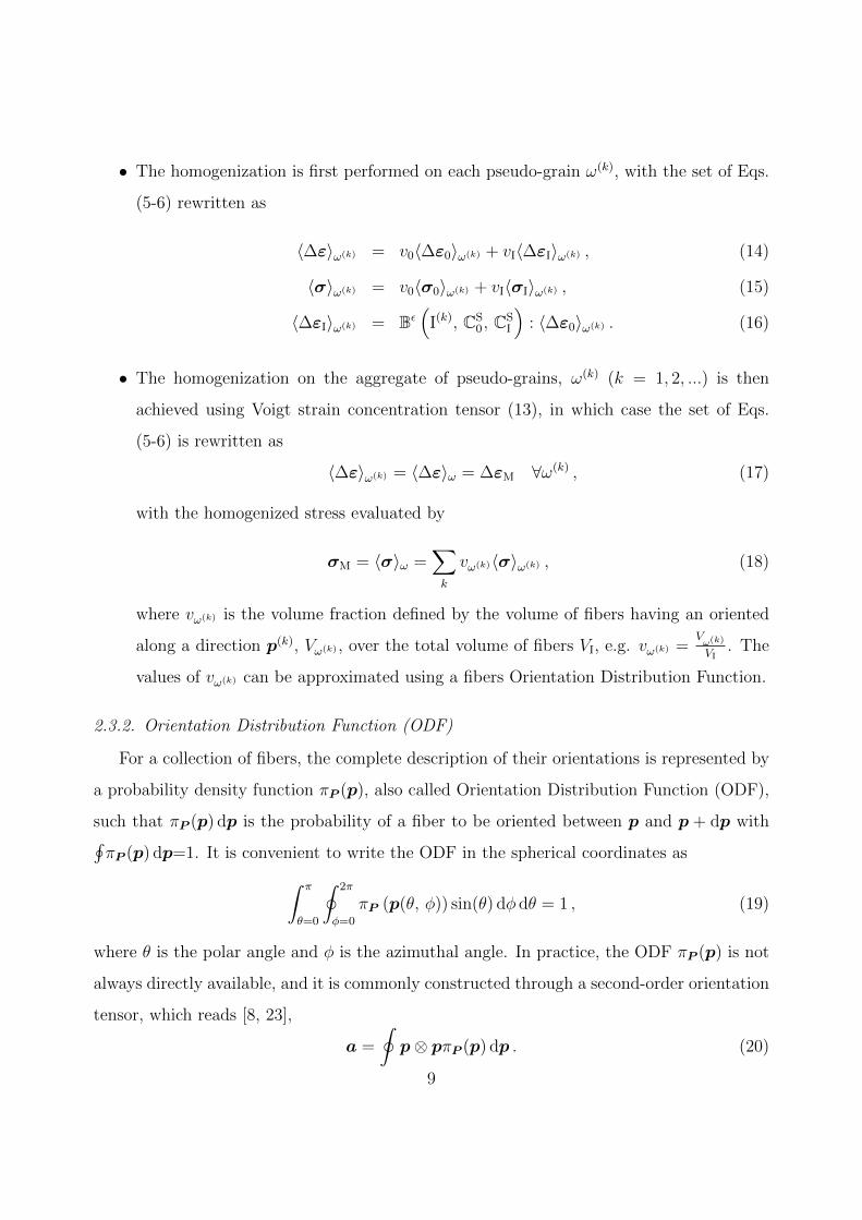
2.3.3. Skin-Core effect

Pseudo grains (𝑘) of layer (l)

𝜋𝑷(𝑙)(𝒑 𝑘 )

2-step Voigt

𝔹𝜀 = 𝕀

ℂM(𝑙)

ℂ0 , ℂI , 𝑣0(𝑙), 𝜋𝑷

(𝑙)𝒑(𝑘)

ℂM ℂ0 , ℂI ; 𝑙 = 0. . 𝑁

Figure 3: Two-step homogenization with skin-core effect: the micro-scale volume element ω is decomposed

into layers (l); each layer is decomposed into pseudo-grains ω(k, l) and its homogenized behavior is obtained

using the 2-step homogenization; the composite behavior is eventually obtained using Voigt assumption on

the different layers.

During the injection molding process, there exists a skin-core effect, in which case the

fiber orientation distribution is not uniform across the plate thickness. In this work, the

10

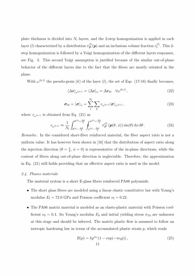
plate thickness is divided into Nl layers, and the 2-step homogenization is applied in each

layer (l) characterized by a distribution π(l)P (p) and an inclusions volume fraction v

(l)I . This 2-

step homogenization is followed by a Voigt homogenization of the different layers responses,

see Fig. 3. This second Voigt assumption is justified because of the similar out-of-plane

behavior of the different layers due to the fact that the fibers are mostly oriented in the

plane.

With ω(k; l) the pseudo-grain (k) of the layer (l), the set of Eqs. (17-18) finally becomes,

〈∆ε〉ω(k; l) = 〈∆ε〉ω = ∆εM ∀ω(k; l) , (22)

σM = 〈σ〉ω =

Nl∑l

∑k

vω(k; l)〈σ〉ω(k; l) , (23)

where vω(k, l) is obtained from Eq. (21) as

vω(k; l) ≈1

Nl

∫ θ(k)+ ∆θ2

θ(k)−∆θ2

∮ φ(k)+ ∆φ2

φ(k)−∆φ2

π(l)P (p(θ, φ)) sin(θ) dφ dθ . (24)

Remarks:. In the considered short-fiber reinforced material, the fiber aspect ratio is not a

uniform value. It has however been shown in [16] that the distribution of aspect ratio along

the injection direction (θ = π2, φ = 0) is representative of the in-plane directions, while the

content of fibers along out-of-plane direction is neglectable. Therefore, the approximation

in Eq. (21) still holds providing that an effective aspect ratio is used in the model.

2.4. Phases materials

The material system is a short E-glass fibers reinforced PA06 polyamide.

• The short glass fibers are modeled using a linear elastic constitutive law with Young’s

modulus EI = 72.0 GPa and Poisson coefficient νI = 0.22.

• The PA06 matrix material is modeled as an elasto-plastic material with Poisson coef-

ficient ν0 = 0.4. Its Young’s modulus E0 and initial yielding stress σY0 are unknown

at this stage and should be inferred. The matrix plastic flow is assumed to follow an

isotropic hardening law in terms of the accumulated plastic strain p, which reads

R(p) = hpm1(1− exp(−m2p)) , (25)

11

where h, m1 and m2 are unknown hardening parameters to be inferred.

The unknown material parameters E0, σY0, h, m1, m2 and the effect of the effective

fiber aspect ratio Ar will be identified by Bayesian Inference (BI) using experimental tests

conducted on composite coupons. Although the presented two-step homogenization is rather

efficient compared to computational homogenization, running this homogenization process

during a BI process with a Metropolis-Hastings (MCMC) random walk is only affordable

in the linear elastic case. Therefore, in order to carry out the BI in the non-linear range, a

Deep Neural Network is adopted as a surrogate model of the two-step homogenization.

3. Deep Neural Network

∑

𝑤1

𝑤𝑘

𝑤𝑛0⬚

𝑥1

𝑥𝑘

𝑥𝑛0⬚

𝑤𝟎 + 𝑤𝑘𝑥𝑘

𝒏𝟎

𝒌=𝟏

𝒇( ∑ )

(a)

𝑥1

𝑥𝑛000

𝑦1

𝑦𝑛𝑁00

𝑛1 𝑛𝑁−1

𝑛𝑖

𝒘𝟏 𝒘𝑵

𝑛0 𝑛𝑁

𝒘01

𝒘0𝑁

𝒘0𝑁−1−

(b)

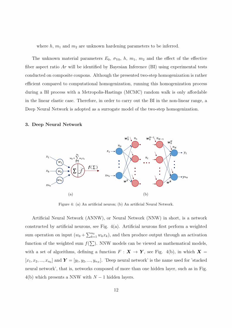
Figure 4: (a) An artificial neuron; (b) An artificial Neural Network.

Artificial Neural Network (ANNW), or Neural Network (NNW) in short, is a network

constructed by artificial neurons, see Fig. 4(a). Artificial neurons first perform a weighted

sum operation on input (w0 +∑n0

k=1wkxk), and then produce output through an activation

function of the weighted sum f(∑

). NNW models can be viewed as mathematical models,

with a set of algorithms, defining a function F : X → Y , see Fig. 4(b), in which X =

[x1, x2, ..., xn0 ] and Y = [y1, y2, ..., ynN ]. ’Deep neural network’ is the name used for ’stacked

neural network’, that is, networks composed of more than one hidden layer, such as in Fig.

4(b) which presents a NNW with N − 1 hidden layers.

12

The training of the NNW refers to regression as supervised learning. Based on a given

set of input-output pairs, supervised learning refers to training the weight parameters wikj,

with i = 1, ..., N ; k = 1, ..., ni−1 and j = 1, ..., ni, and bias wi0j , with i = 1, ..., N and j =

1, ..., ni, see the notations in Fig. 4(b), and making the NNW being able to map input

to corresponding output. A loss function is defined to measure the difference between the

predicted output YYY and given output YYY , such as floss = 12‖YYY − YYY ‖2, where ‖ • ‖ refers to

the Frobenius norm. Deep learning can be carried out by back-propagation, which updates

the values of wikj iteratively to minimize the loss function floss. To this end, the Python

library ’Scikit-learn’ for NNW regression [24] is used in this work. The architecture of the

NNW is obtained by following a trying process: i) starting from a simple architecture; ii)

increasing the depth of the network (the number of hidden layers) progressively; and iii)

monitoring the improvement of the NNW. The hyperbolic tangent function ’tanh’ is chosen

as the activation function.

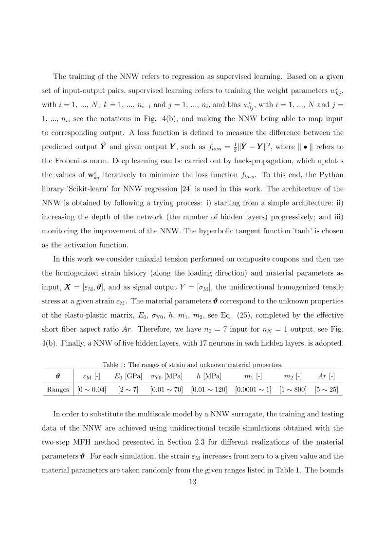
In this work we consider uniaxial tension performed on composite coupons and then use

the homogenized strain history (along the loading direction) and material parameters as

input, XXX = [εM,ϑϑϑ], and as signal output Y = [σM], the unidirectional homogenized tensile

stress at a given strain εM. The material parameters ϑϑϑ correspond to the unknown properties

of the elasto-plastic matrix, E0, σY0, h, m1, m2, see Eq. (25), completed by the effective

short fiber aspect ratio Ar. Therefore, we have n0 = 7 input for nN = 1 output, see Fig.

4(b). Finally, a NNW of five hidden layers, with 17 neurons in each hidden layers, is adopted.

Table 1: The ranges of strain and unknown material properties.

ϑϑϑ εM [-] E0 [GPa] σY0 [MPa] h [MPa] m1 [-] m2 [-] Ar [-]

Ranges [0 ∼ 0.04] [2 ∼ 7] [0.01 ∼ 70] [0.01 ∼ 120] [0.0001 ∼ 1] [1 ∼ 800] [5 ∼ 25]

In order to substitute the multiscale model by a NNW surrogate, the training and testing

data of the NNW are achieved using unidirectional tensile simulations obtained with the

two-step MFH method presented in Section 2.3 for different realizations of the material

parameters ϑϑϑ. For each simulation, the strain εM increases from zero to a given value and the

material parameters are taken randomly from the given ranges listed in Table 1. The bounds

13

of E0 and Ar are chosen with respect to the identification process conducted [16] for the

same material system, but limited to the linear range, in which the inferred values are within

these ranges. The bounds of the other parameters correspond to extreme values by lack of

prior knowledge. During each simulation, 70 strain-stress points are recorded: together with

the material parameters, they correspond to 70 input and output data pairs of the NNW.

Only a few hundreds of simulations (typically < 500) were needed for the designed NNW to

be trained (i.e. the mean squared error is lower than 0.5×10−4). Compared to the hundreds

of thousands of simulations required for a MCMC random walk, the total computation time

is reduced drastically.

4. Experimental tests

0O

45O

90O

19

67.74

38.10

13

(a) Coupons

0.00 0.01 0.02 0.03 0.04M

0

50

100

150

in M

Pa

0-Degree45-Degree90-Degree

(b) Uniaxial strain-stress curves

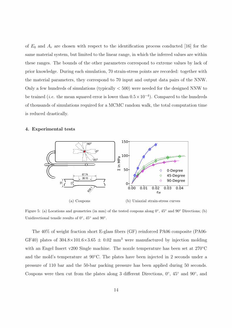
Figure 5: (a) Locations and geometries (in mm) of the tested coupons along 0◦, 45◦ and 90◦ Directions; (b)

Unidirectional tensile results of 0◦, 45◦ and 90◦.

The 40% of weight fraction short E-glass fibers (GF) reinforced PA06 composite (PA06-

GF40) plates of 304.8×101.6×3.65 ± 0.02 mm3 were manufactured by injection molding

with an Engel Insert v200 Single machine. The nozzle temperature has been set at 270◦C

and the mold’s temperature at 90◦C. The plates have been injected in 2 seconds under a

pressure of 110 bar and the 50-bar packing pressure has been applied during 50 seconds.

Coupons were then cut from the plates along 3 different Directions, 0◦, 45◦ and 90◦, and

14

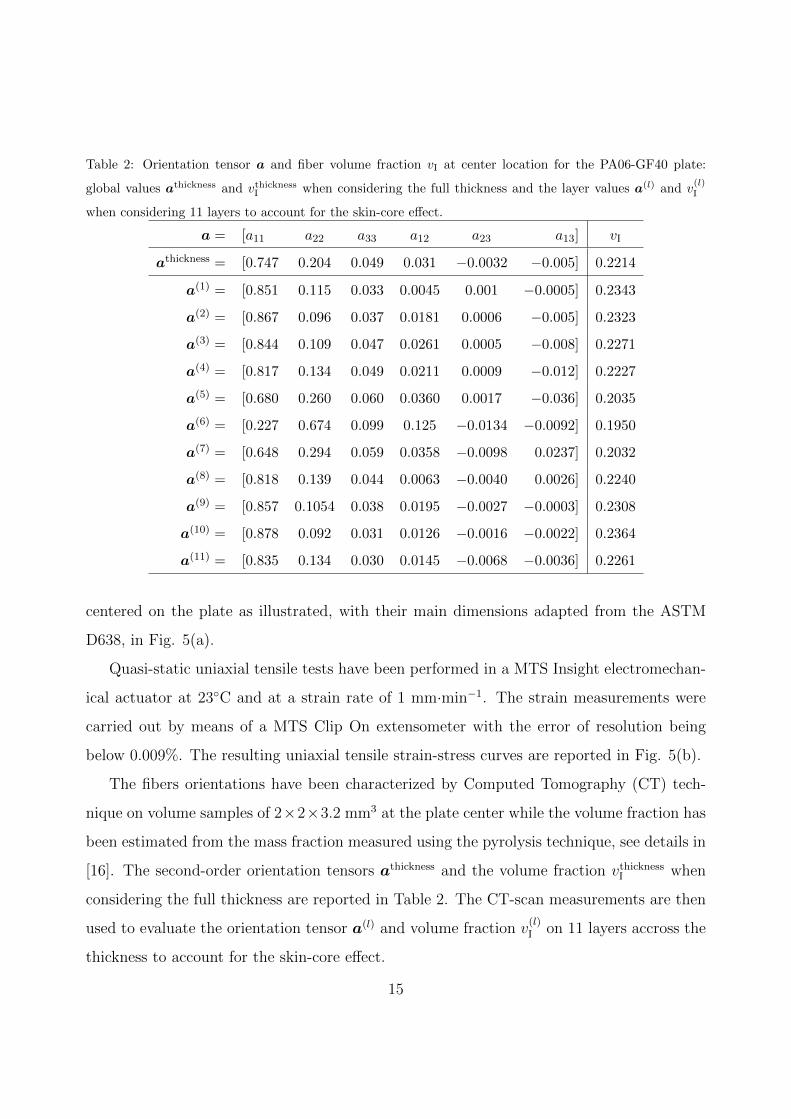
Table 2: Orientation tensor a and fiber volume fraction vI at center location for the PA06-GF40 plate:

global values athickness and vthicknessI when considering the full thickness and the layer values a(l) and v(l)I

when considering 11 layers to account for the skin-core effect.

a = [a11 a22 a33 a12 a23 a13] vI

athickness = [0.747 0.204 0.049 0.031 −0.0032 −0.005] 0.2214

a(1) = [0.851 0.115 0.033 0.0045 0.001 −0.0005] 0.2343

a(2) = [0.867 0.096 0.037 0.0181 0.0006 −0.005] 0.2323

a(3) = [0.844 0.109 0.047 0.0261 0.0005 −0.008] 0.2271

a(4) = [0.817 0.134 0.049 0.0211 0.0009 −0.012] 0.2227

a(5) = [0.680 0.260 0.060 0.0360 0.0017 −0.036] 0.2035

a(6) = [0.227 0.674 0.099 0.125 −0.0134 −0.0092] 0.1950

a(7) = [0.648 0.294 0.059 0.0358 −0.0098 0.0237] 0.2032

a(8) = [0.818 0.139 0.044 0.0063 −0.0040 0.0026] 0.2240

a(9) = [0.857 0.1054 0.038 0.0195 −0.0027 −0.0003] 0.2308

a(10) = [0.878 0.092 0.031 0.0126 −0.0016 −0.0022] 0.2364

a(11) = [0.835 0.134 0.030 0.0145 −0.0068 −0.0036] 0.2261

centered on the plate as illustrated, with their main dimensions adapted from the ASTM

D638, in Fig. 5(a).

Quasi-static uniaxial tensile tests have been performed in a MTS Insight electromechan-

ical actuator at 23◦C and at a strain rate of 1 mm·min−1. The strain measurements were

carried out by means of a MTS Clip On extensometer with the error of resolution being

below 0.009%. The resulting uniaxial tensile strain-stress curves are reported in Fig. 5(b).

The fibers orientations have been characterized by Computed Tomography (CT) tech-

nique on volume samples of 2×2×3.2 mm3 at the plate center while the volume fraction has

been estimated from the mass fraction measured using the pyrolysis technique, see details in

[16]. The second-order orientation tensors athickness and the volume fraction vthicknessI when

considering the full thickness are reported in Table 2. The CT-scan measurements are then

used to evaluate the orientation tensor a(l) and volume fraction v(l)I on 11 layers accross the

thickness to account for the skin-core effect.

15

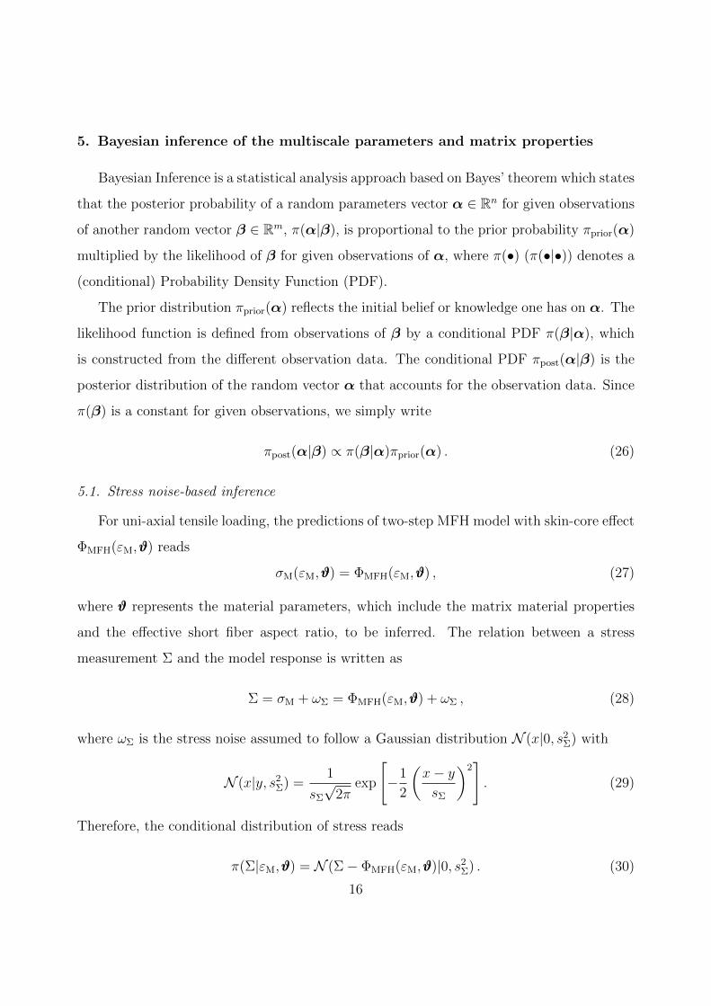
5. Bayesian inference of the multiscale parameters and matrix properties

Bayesian Inference is a statistical analysis approach based on Bayes’ theorem which states

that the posterior probability of a random parameters vector α ∈ Rn for given observations

of another random vector β ∈ Rm, π(α|β), is proportional to the prior probability πprior(α)

multiplied by the likelihood of β for given observations of α, where π(•) (π(•|•)) denotes a

(conditional) Probability Density Function (PDF).

The prior distribution πprior(α) reflects the initial belief or knowledge one has on α. The

likelihood function is defined from observations of β by a conditional PDF π(β|α), which

is constructed from the different observation data. The conditional PDF πpost(α|β) is the

posterior distribution of the random vector α that accounts for the observation data. Since

π(β) is a constant for given observations, we simply write

πpost(α|β) ∝ π(β|α)πprior(α) . (26)

5.1. Stress noise-based inference

For uni-axial tensile loading, the predictions of two-step MFH model with skin-core effect

ΦMFH(εM,ϑϑϑ) reads

σM(εM,ϑϑϑ) = ΦMFH(εM,ϑϑϑ) , (27)

where ϑϑϑ represents the material parameters, which include the matrix material properties

and the effective short fiber aspect ratio, to be inferred. The relation between a stress

measurement Σ and the model response is written as

Σ = σM + ωΣ = ΦMFH(εM,ϑϑϑ) + ωΣ , (28)

where ωΣ is the stress noise assumed to follow a Gaussian distribution N (x|0, s2Σ) with

N (x|y, s2Σ) =

1

sΣ

√2π

exp

[−1

2

(x− ysΣ

)2]. (29)

Therefore, the conditional distribution of stress reads

π(Σ|εM,ϑϑϑ) = N (Σ− ΦMFH(εM,ϑϑϑ)|0, s2Σ) . (30)

16

No

Direct Mean field homogenization simulations with uniaxial tensile strain εM increasing from 0 to 0.04. Material properties 𝝑 = [E0, σY0, h, m1, m2, Ar]

0-degree, with random

material properties 𝝑

Training of NNW0

Input: εM, 𝝑

Output: σM

45-degree with random

material properties 𝝑

90-degree with random

material properties 𝝑

Training of NNW45

Input: εM, 𝝑

Output: σM

Training of NNW90

Input: εM, 𝝑

Output: σM

Box 1: Mean Field Homogenization (MFH) and Neural Network (NNW)

Trained NNWs:

NNW0

NNW45

NNW90

Initialize sample 𝝑𝟎 ∈ ℝ𝟔, k=0; total number of samples N

Box 2: Bayesian Inference (BI) and Markov Chain Monte Carlo

(MCMC) random walking

𝜀𝑖0, 𝜀𝑖

45, 𝜀𝑖90, 𝝑𝒑 (i= 1, …, 𝑛𝑑

po)

If k=0: 𝝑𝒑 = 𝝑𝟎 ;

Else: Draw a sample 𝝑𝒑 ∈ ℝ𝟔 from conditional distribution

𝑝 𝝑𝒑 𝝑𝟎 according to Markov chain process

ΦNNW0 (𝜀𝑖

0, 𝝑𝒑), ΦNNW45 (𝜀𝑖

45, 𝝑𝒑),

ΦNNW90 (𝜀𝑖

90, 𝝑𝒑), (i= 1, …, 𝑛𝑑po

)

𝝑𝟎 = 𝝑𝒑

k=N ?

No

Yes End

k=0 ? Yes

No

k=k+1

Draw a random variable 𝑟 from uniform distribution 𝒰(0, 1).

𝜋 𝚺 𝜺M, 𝝑𝒑 𝜋prior( 𝝑𝒑)

𝜋(𝚺 𝜺M, 𝝑𝟎)𝜋prior(𝝑𝟎) > 𝑟 ?

Yes

Compute the likelihood function 𝜋 𝚺 𝜺M, 𝝑𝒑

using Eq. (32), and 𝜋prior(𝝑𝒑) using Eq. (34)

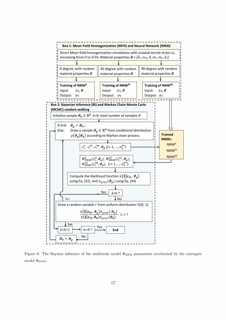
Figure 6: The Baysian inference of the multiscale model ΦMFH parameters accelerated by the surrogate

model ΦNNW.

17

5.2. Bayesian inference using the surrogate model

Since the computational time of the two-step MFH process makes a MCMC sampling

unaffordable, in particular when accounting for the skin-core effect, NNW is used as a

surrogate ΦNNW of MFH model ΦMFH in order to perform the BI, see Fig. 6.

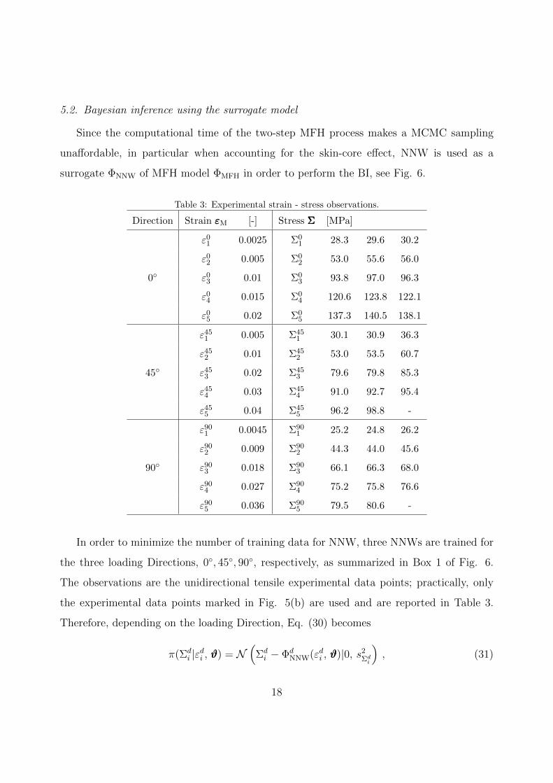
Table 3: Experimental strain - stress observations.

Direction Strain εεεM [-] Stress ΣΣΣ [MPa]

ε01 0.0025 Σ0

1 28.3 29.6 30.2

ε02 0.005 Σ0

2 53.0 55.6 56.0

0◦ ε03 0.01 Σ0

3 93.8 97.0 96.3

ε04 0.015 Σ0

4 120.6 123.8 122.1

ε05 0.02 Σ0

5 137.3 140.5 138.1

ε451 0.005 Σ45

1 30.1 30.9 36.3

ε452 0.01 Σ45

2 53.0 53.5 60.7

45◦ ε453 0.02 Σ45

3 79.6 79.8 85.3

ε454 0.03 Σ45

4 91.0 92.7 95.4

ε455 0.04 Σ45

5 96.2 98.8 -

ε901 0.0045 Σ90

1 25.2 24.8 26.2

ε902 0.009 Σ90

2 44.3 44.0 45.6

90◦ ε903 0.018 Σ90

3 66.1 66.3 68.0

ε904 0.027 Σ90

4 75.2 75.8 76.6

ε905 0.036 Σ90

5 79.5 80.6 -

In order to minimize the number of training data for NNW, three NNWs are trained for

the three loading Directions, 0◦, 45◦, 90◦, respectively, as summarized in Box 1 of Fig. 6.

The observations are the unidirectional tensile experimental data points; practically, only

the experimental data points marked in Fig. 5(b) are used and are reported in Table 3.

Therefore, depending on the loading Direction, Eq. (30) becomes

π(Σdi |εdi , ϑϑϑ) = N

(Σdi − Φd

NNW(εdi , ϑϑϑ)|0, s2Σdi

), (31)

18

where the superscript d = 0, 45, 90 refers to the tensile loading and coupon Direction,

and where the subscript i is used to indicate the stress variance sΣdiobtained from the

experimental curves at a given strain εdi , the subscript “M” being omitted for conciseness.

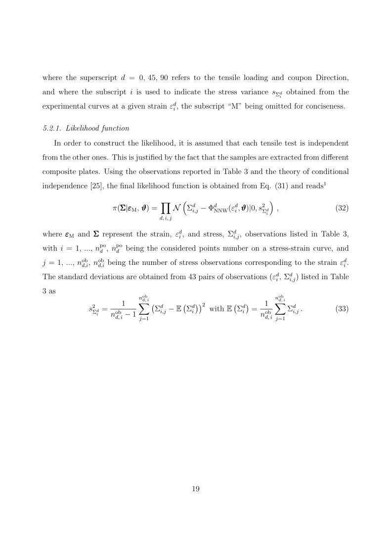
5.2.1. Likelihood function

In order to construct the likelihood, it is assumed that each tensile test is independent

from the other ones. This is justified by the fact that the samples are extracted from different

composite plates. Using the observations reported in Table 3 and the theory of conditional

independence [25], the final likelihood function is obtained from Eq. (31) and reads1

π(ΣΣΣ|εεεM, ϑϑϑ) =∏d, i, j

N(

Σdi,j − Φd

NNW(εdi ,ϑϑϑ)|0, s2Σdi

), (32)

where εεεM and ΣΣΣ represent the strain, εdi , and stress, Σdi,j, observations listed in Table 3,

with i = 1, ..., npod , npo

d being the considered points number on a stress-strain curve, and

j = 1, ..., nobd,i, n

obd,i being the number of stress observations corresponding to the strain εdi .

The standard deviations are obtained from 43 pairs of observations (εdi , Σdi,j) listed in Table

3 as

s2Σdi

=1

nobd, i − 1

nobd, i∑j=1

(Σdi,j − E

(Σdi

))2with E

(Σdi

)=

1

nobd, i

nobd, i∑j=1

Σdi,j . (33)

19

3 4 5 6E0 in GPa

0.0

0.2

0.4

0.6

0.8

Prob

abilit

y

e6.4, 11.3, 2.4, 6.5

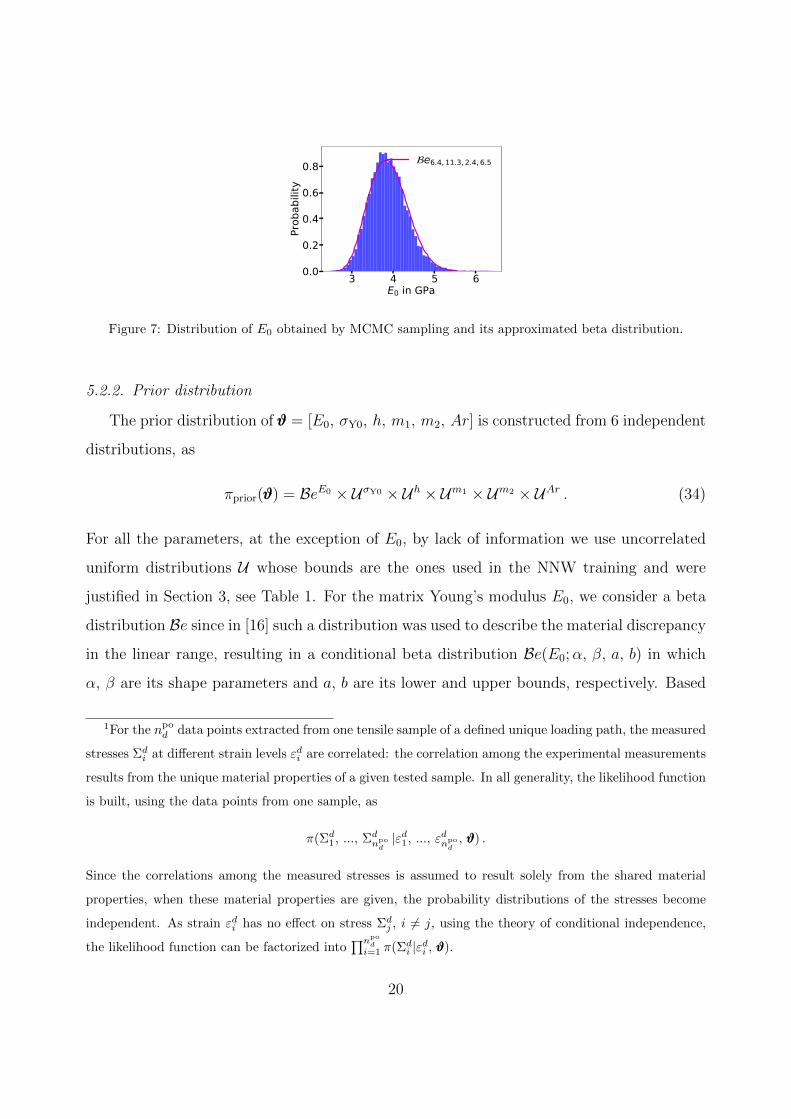
Figure 7: Distribution of E0 obtained by MCMC sampling and its approximated beta distribution.

5.2.2. Prior distribution

The prior distribution of ϑϑϑ = [E0, σY0, h, m1, m2, Ar] is constructed from 6 independent

distributions, as

πprior(ϑϑϑ) = BeE0 × UσY0 × Uh × Um1 × Um2 × UAr . (34)

For all the parameters, at the exception of E0, by lack of information we use uncorrelated

uniform distributions U whose bounds are the ones used in the NNW training and were

justified in Section 3, see Table 1. For the matrix Young’s modulus E0, we consider a beta

distribution Be since in [16] such a distribution was used to describe the material discrepancy

in the linear range, resulting in a conditional beta distribution Be(E0;α, β, a, b) in which

α, β are its shape parameters and a, b are its lower and upper bounds, respectively. Based

1For the npod data points extracted from one tensile sample of a defined unique loading path, the measured

stresses Σdi at different strain levels εdi are correlated: the correlation among the experimental measurements

results from the unique material properties of a given tested sample. In all generality, the likelihood function

is built, using the data points from one sample, as

π(Σd1, ..., Σd

npod|εd1, ..., εdnpo

d, ϑϑϑ) .

Since the correlations among the measured stresses is assumed to result solely from the shared material

properties, when these material properties are given, the probability distributions of the stresses become

independent. As strain εdi has no effect on stress Σdj , i 6= j, using the theory of conditional independence,

the likelihood function can be factorized into∏npo

di=1 π(Σd

i |εdi , ϑϑϑ).

20

on this conditional distribution of E0, we have

π(E0) =

∫α, β, a, c

Be(E0;α, β, a, c)π(α, β, a, b)dα dβ da db , (35)

where the distributions of α, β, a, b were inferred in [16] from experimental tests. Their inte-

gration in Eq. (35) is carried out using a MCMC sampling, and the resulting marginal distri-

bution is eventually approximated by a beta distribution Be(E0|6.4, 11.3, 2.4 GPa, 6.5 GPa),

see Fig. 7, which serves as the prior distribution of E0.

5.2.3. Posterior distribution

Finally, the posterior distribution

πpost(ϑϑϑ|εεεM, ΣΣΣ) ∝ π(ΣΣΣ|εεεM, ϑϑϑ)πprior(ϑϑϑ) , (36)

is evaluated using a MCMC technique, which is a random walk in the parameter space

ϑ ∈ R7, as summarized in Box 2 of Fig. 6. The adaptive variant [26] of the Metropolis

algorithm [27] is used, see also [16] for details.

6. Results and Discussion

In this section, we first ascertain the convergence of the BI before providing the posterior

distribution obtained by the NNW-accelerated BI. We also show that considering the NNW

as surrogate during the BI does not impact on the accuracy. Finally we show that, while

the NNW-accelerated BI is manageable, using directly the two-step MFH during the BI is

computationally unaffordable.

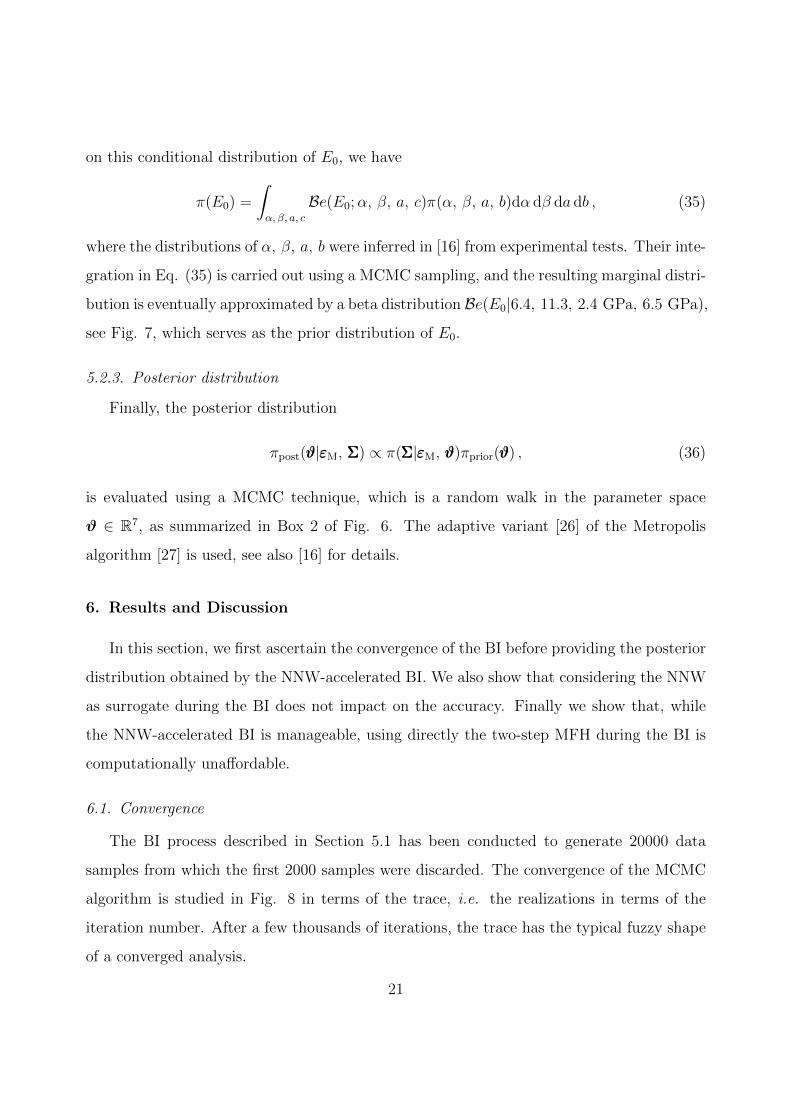
6.1. Convergence

The BI process described in Section 5.1 has been conducted to generate 20000 data

samples from which the first 2000 samples were discarded. The convergence of the MCMC

algorithm is studied in Fig. 8 in terms of the trace, i.e. the realizations in terms of the

iteration number. After a few thousands of iterations, the trace has the typical fuzzy shape

of a converged analysis.

21

5000 6000 7000 8000 9000 10000iteration

0.25

0.50

0.75

1.00

1.25

1.50

1.75/

[]

E0 m1 h

(a)

5000 6000 7000 8000 9000 10000iteration

0.6

0.7

0.8

0.9

1.0

1.1

1.2

/[

]

m2 Y0 Ar

(b)

Figure 8: Trace of the inferred parameters with respect to the MCMC iteration

H

M

L

ℎ 𝜎Y0 𝑚1

(MPa)

( - )

( - )

( - )

𝑚2

𝐴𝑟

𝐸0

ℎ

𝜎Y0

𝑚1

𝑚2

(GPa)

(MPa)

(MPa)

(MPa)

( - )

( - )

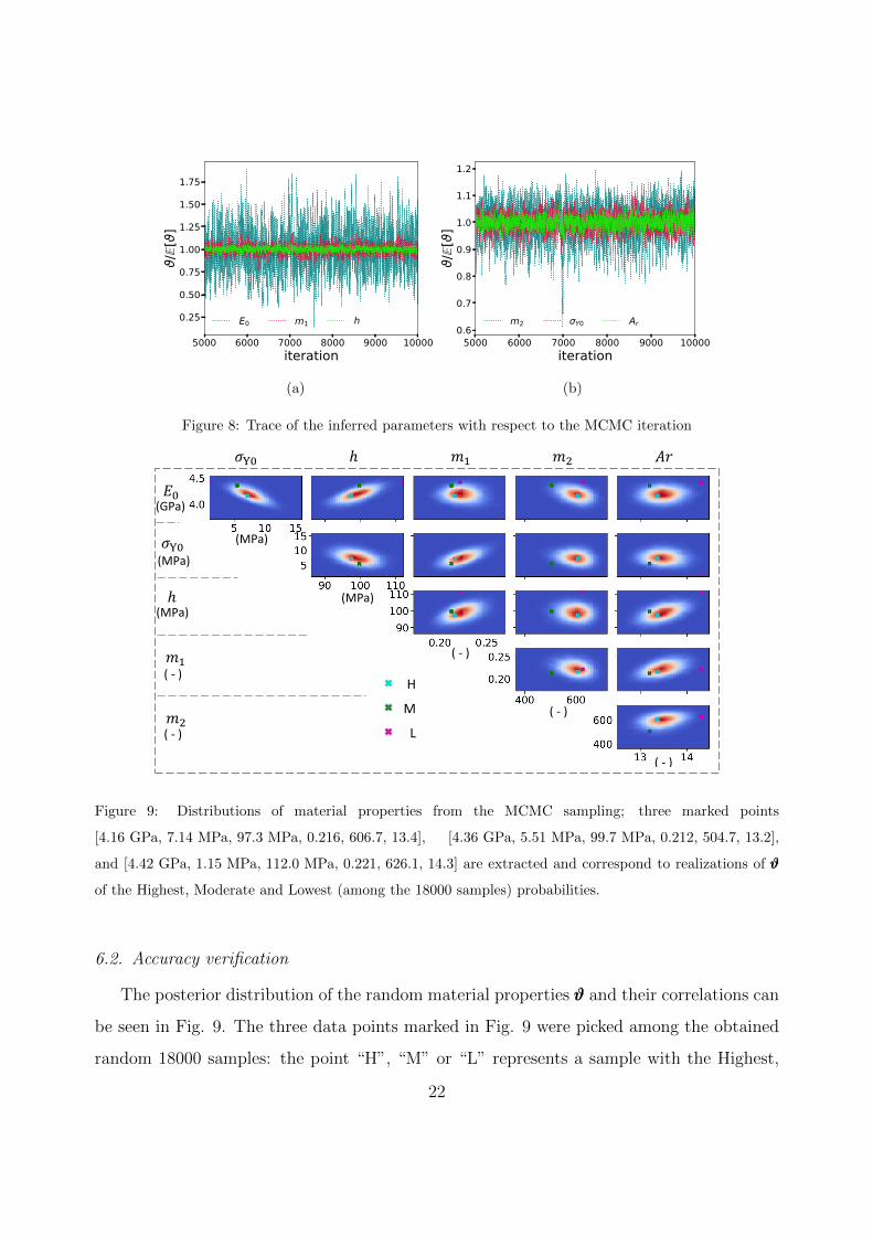
Figure 9: Distributions of material properties from the MCMC sampling; three marked points

[4.16 GPa, 7.14 MPa, 97.3 MPa, 0.216, 606.7, 13.4], [4.36 GPa, 5.51 MPa, 99.7 MPa, 0.212, 504.7, 13.2],

and [4.42 GPa, 1.15 MPa, 112.0 MPa, 0.221, 626.1, 14.3] are extracted and correspond to realizations of ϑϑϑ

of the Highest, Moderate and Lowest (among the 18000 samples) probabilities.

6.2. Accuracy verification

The posterior distribution of the random material properties ϑϑϑ and their correlations can

be seen in Fig. 9. The three data points marked in Fig. 9 were picked among the obtained

random 18000 samples: the point “H”, “M” or “L” represents a sample with the Highest,

22

0.00 0.01 0.02 0.03 0.04M

0

20

40

60

80

100

120

140 in

MPa

Experiments NNW

(a) NNW

0.00 0.01 0.02 0.03 0.04M

0

20

40

60

80

100

120

140

in M

Pa

ExperimentsTwo-step homogenization

(b) Two-step homogenization

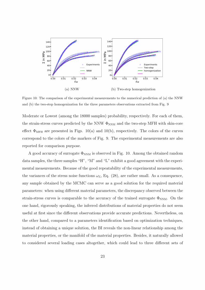
Figure 10: The comparison of the experimental measurements to the numerical prediction of (a) the NNW

and (b) the two-step homogenization for the three parameters observations extracted from Fig. 9

Moderate or Lowest (among the 18000 samples) probability, respectively. For each of them,

the strain-stress curves predicted by the NNW ΦNNM and the two-step MFH with skin-core

effect ΦMFH are presented in Figs. 10(a) and 10(b), respectively. The colors of the curves

correspond to the colors of the markers of Fig. 9. The experimental measurements are also

reported for comparison purpose.

A good accuracy of surrogate ΦNNM is observed in Fig. 10. Among the obtained random

data samples, the three samples “H”, “M” and “L” exhibit a good agreement with the experi-

mental measurements. Because of the good repeatability of the experimental measurements,

the variances of the stress noise functions ωΣ, Eq. (28), are rather small. As a consequence,

any sample obtained by the MCMC can serve as a good solution for the required material

parameters: when using different material parameters, the discrepancy observed between the

strain-stress curves is comparable to the accuracy of the trained surrogate ΦNNM. On the

one hand, rigorously speaking, the inferred distributions of material properties do not seem

useful at first since the different observations provide accurate predictions. Nevertheless, on

the other hand, compared to a parameters identification based on optimization techniques,

instead of obtaining a unique solution, the BI reveals the non-linear relationship among the

material properties, or the manifold of the material properties. Besides, it naturally allowed

to considered several loading cases altogether, which could lead to three different sets of

23

parameters for a deterministic inverse identification.

Nevertheless, in this paper, the micro-mechanical model is seen as deterministic: al-

though some uncertainties exist in the identified parameters the multiscale model is not able

to represent the observed dispersion in the materials. However, in the case of polymeric-

based composites, such dispersion can be important: in [28], PA06 tensile modulus measured

at at constant temperature and strain rate ranges from 1200 to 3400 MPa, and tensile tests

conducted on PA06-GF30 lead to a Young’s modulus ranging from 6200 to 9500 MPa. To

capture this dispersion, properties spatial distributions can be inferred [29], or BI can be

adapted in order to infer the parameters of an assumed distribution of the material proper-

ties instead of the material properties themselves [30]. This so-called distribution-based BI

approach requires a double MCMC sampling process in the non-linear range, which is the

reason why in [16] the authors have inferred the distribution of the linear material constants

only. However, because of the high efficiency, see next subsection, of the NNW, such an ap-

proach would become affordable to infer the parameters distribution of elasto-(visco)-plastic

composites multiscale models.

6.3. Computational efficiency

Table 4 compares the computational time needed to perform a direct BI, which uses

the 2-step MFH model ΦMFH to evaluate the likelihood, to the time to perform the NNW-

accelerated BI, which uses the surrogate model ΦNNW when evaluating the likelihood. For the

NNW-accelerated BI, an offline computation is required. Data needs first to be generated,

which consists in running 500 times the 2-step MFH model ΦMFH along 3 loading directions.

Although this requires roughly 2 days of computations, this can be perform in parallel

since the simulations are independent. The NNW then needs to be trained for each loading

direction, requiring half an hour. The total offline time si thus about 2 days. To perform the

BI, for each accepted sample, the MCMC algorithm rejects between 10 and 20000 samples.

It is estimated that 6 millions evaluations of the likelihood are required to reach the converge

posterior (we note that a rejected sample requires the evaluation of the likelihood). Since

evaluating the surrogate model ΦNNW is almost instantaneous, the NNW-accelerated BI

24

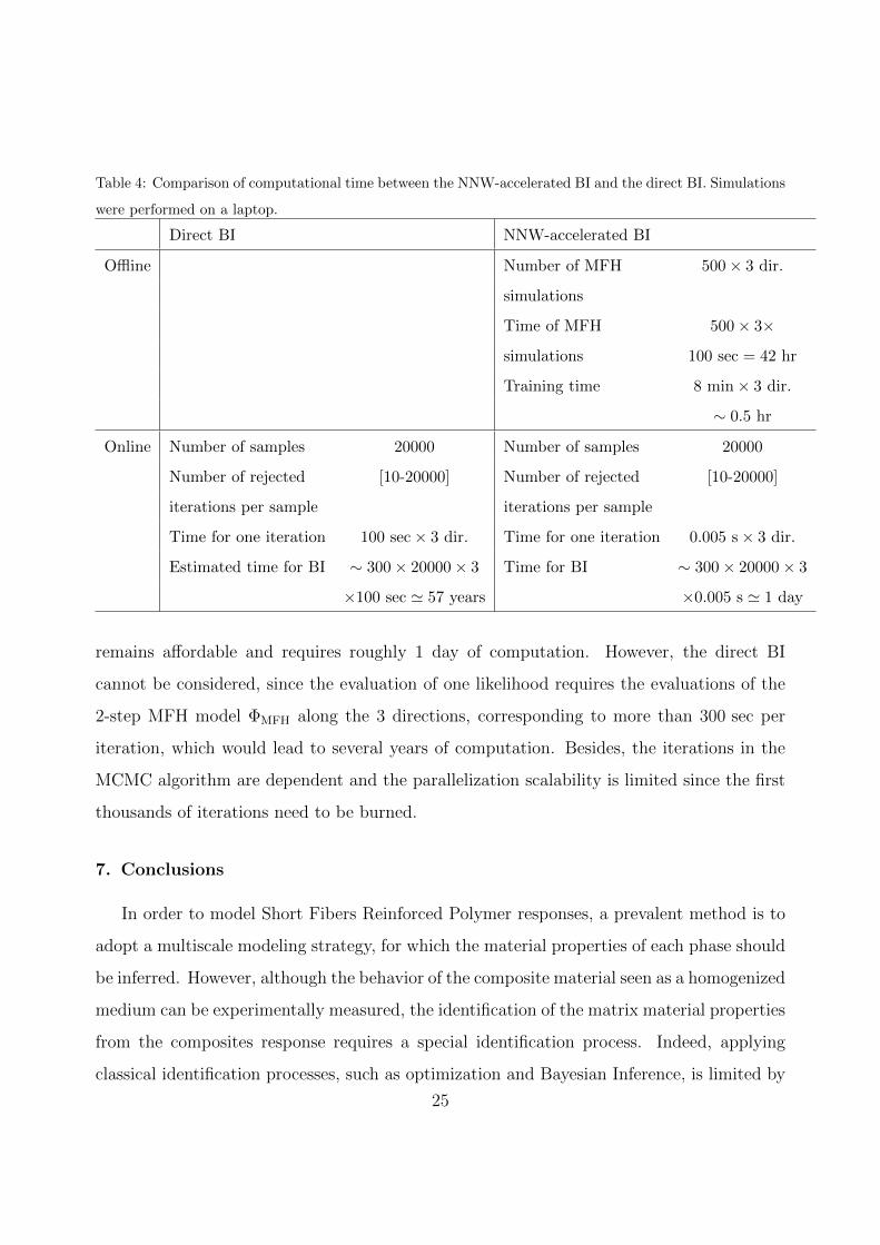
Table 4: Comparison of computational time between the NNW-accelerated BI and the direct BI. Simulations

were performed on a laptop.

Direct BI NNW-accelerated BI

Offline Number of MFH 500× 3 dir.

simulations

Time of MFH 500× 3×

simulations 100 sec = 42 hr

Training time 8 min× 3 dir.

∼ 0.5 hr

Online Number of samples 20000 Number of samples 20000

Number of rejected [10-20000] Number of rejected [10-20000]

iterations per sample iterations per sample

Time for one iteration 100 sec× 3 dir. Time for one iteration 0.005 s× 3 dir.

Estimated time for BI ∼ 300× 20000× 3 Time for BI ∼ 300× 20000× 3

×100 sec ' 57 years ×0.005 s ' 1 day

remains affordable and requires roughly 1 day of computation. However, the direct BI

cannot be considered, since the evaluation of one likelihood requires the evaluations of the

2-step MFH model ΦMFH along the 3 directions, corresponding to more than 300 sec per

iteration, which would lead to several years of computation. Besides, the iterations in the

MCMC algorithm are dependent and the parallelization scalability is limited since the first

thousands of iterations need to be burned.

7. Conclusions

In order to model Short Fibers Reinforced Polymer responses, a prevalent method is to

adopt a multiscale modeling strategy, for which the material properties of each phase should

be inferred. However, although the behavior of the composite material seen as a homogenized

medium can be experimentally measured, the identification of the matrix material properties

from the composites response requires a special identification process. Indeed, applying

classical identification processes, such as optimization and Bayesian Inference, is limited by

25

the complexity of the micromechanics models, especially for non-linear cases in which multi-

parameters are involved and for which the computation cost is not negligible. In particular,

when considering a two-step homogenization as a non-linear multiscale model, the MCMC

sampling of a BI process becomes unaffordable.

In this paper, a NNW was adopted as a surrogate model to replace the expensive mi-

cromechanics model during the material parameters identification process. The accuracy of

NNW was verified from the comparison between the strain stress curves obtained with NNW

and those obtained by the two-step homogenization. The matrix material properties and

the effective fiber aspect ratio were then identified by the BI process from the experimental

measurements on composite coupons. In particular, it was shown that the inferred prop-

erties could predict the composite material response in agreement with the experimental

curves.

Although the methodology was developed for a particular homogenization method, i.e.

MFH, it can be extended to other ones, such as computational homogenization, or to more

complex identification tests. For example, the method can be applied for multi-axial stress-

strain cases, assuming a monotonicand proportional loading, in which case a strain vector

–of size up to 6– serves as inputs, together with the material parameters, of the NNW instead

of a ingle strain variable; the corresponding –up to 6– outputs will be used to represent the

stress vector. Consequently, since the number of inputs is increased, the adopted structure

of the NNW needs to be enhanced by more hidden layers and neurons to be able to represent

a more complicated high dimensional nonlinear mapping. As a result of the enhancement of

the NNW, an increased number of training data would probably be required. On the aspect

of BI process, the original uni-variate Gaussian distribution used to construct the likelihood

function has to be replaced by a multivariate Gaussian distribution of higher dimension

–up to 6, and the different importance of the stress entries can be addressed by using a

modified precision matrix in the multivariate Gaussian distribution. Finally, in order to

introduce some stochasticity in the multiscale model, it is foreseen to infer the parameters

of an assumed distribution of the material properties instead of the material properties

themselves. Because this so-called distribution-based BI approach requires a double MCMC

26

sampling process in the non-linear range, the method is not practical with direct BI for a

complex micro-mechanical model. However, because of the high efficiency of the NNW, this

becomes possible in the cases of elasto-(visco)-plastic composites.

Acknowledgment. The research has been funded by the Walloon Region under the agree-

ment no 1410246-STOMMMAC (CT-INT 2013-03-28), by the Gaitek 2015 programm of

the Basque Government, and by the Austrian Research Promotion Agency (ffg) under the

agreement no 850392 (STOMMMAC) in the context of the M-ERA.NET Joint Call 2014.

References

[1] K. Matous, M. G. Geers, V. G. Kouznetsova, A. Gillman, A review of predictive nonlinear theories for

multiscale modeling of heterogeneous materials, Journal of Computational Physics 330 (Supplement C)

(2017) 192 – 220, doi:10.1016/j.jcp.2016.10.070.

[2] J. D. Eshelby, The Determination of the Elastic Field of an Ellipsoidal Inclusion, and Related Problems,

Proceedings of the Royal Society of London. Series A 241 (1226) (1957) 376–396.

[3] T. Mori, K. Tanaka, Average stress in matrix and average elastic energy of materials with misfitting

inclusions, Acta Metallurgica 21 (5) (1973) 571–574.

[4] R. Hill, Continuum micro-mechanics of elastoplastic polycrystals, Journal of the Mechanics and Physics

of Solids 13 (2) (1965) 89 – 101, doi:10.1016/0022-5096(65)90023-2.

[5] D. R. S. Talbot, J. R. Willis, Variational Principles for Inhomogeneous Non-linear Media, IMA Journal

of Applied Mathematics 35 (1) (1985) 39–54.

[6] L. Wu, L. Noels, L. Adam, I. Doghri, A combined incremental–secant mean–field homogenization

scheme with per–phase residual strains for elasto–plastic composites, International Journal of Plasticity

51 (2013) 80–102, doi:10.1016/j.ijplas.2013.06.006.

[7] C. W. Camacho, C. L. Tucker, S. Yalva c, R. L. McGee, Stiffness and thermal expansion predictions for

hybrid short fiber composites, Polymer Composites 11 (4) (1990) 229–239, doi:10.1002/pc.750110406.

[8] I. Doghri, L. Tinel, Micromechanics of inelastic composites with misaligned inclusions: Numerical

treatment of orientation, Computer Methods in Applied Mechanics and Engineering 195 (13) (2006)

1387 – 1406, doi:10.1016/j.cma.2005.05.041.

[9] M. Vincent, T. Giroud, A. Clarke, C. Eberhardt, Description and modeling of fiber orientation in

injection molding of fiber reinforced thermoplastics, Polymer 46 (17) (2005) 6719 – 6725.

[10] J. L. Beck, L. S. Katafygiotis, Updating Models and Their Uncertainties. I: Bayesian Statistical Frame-

work, Journal of Engineering Mechanics 124 (1998) 455–461.

27

[11] T. Most, Identification of the parameters of complex constitutive models: Least squares minimization

vs. Bayesian updating, in: D. Straub (Ed.), Reliability and Optimization of Structural Systems, 2010.

[12] S. Madireddy, B. Sista, K. Vemaganti, A Bayesian approach to selecting hyperelastic constitutive

models of soft tissue, Computer Methods in Applied Mechanics and Engineering 291 (2015) 102 – 122,

doi:10.1016/j.cma.2015.03.012.

[13] H. Rappel, L. Beex, J. Hale, L. Noels, S. Bordas, A tutorial on Bayesian inference to identify material

parameters in solid mechanics, Archives of Computational Methods in Engineering doi:10.1007/s11831-

018-09311-x.

[14] T. C. Lai, K. Ip, Parameter estimation of orthotropic plates by Bayesian sensitivity analysis, Composite

Structures 34 (1) (1996) 29 – 42, doi:10.1016/0263-8223(95)00128-X.

[15] F. Daghia, S. de Miranda, F. Ubertini, E. Viola, Estimation of elastic constants of thick lam-

inated plates within a Bayesian framework, Composite Structures 80 (3) (2007) 461 – 473, doi:

10.1016/j.compstruct.2006.06.030.

[16] M. Mohamedou, K. Z. Uriondo, C. N. Chung, H. Rappel, L. Beex, L. Adam, Z. Major, L. Wu, L. Noels,

Bayesian Identification of Mean-Field Homogenization model parameters and uncertain matrix behavior

in non-aligned short fiber composites, Composite Structures Submitted.

[17] B. A. Le, J. Yvonnet, Q.-C. He, Computational homogenization of nonlinear elastic materials using

neural networks, International Journal for Numerical Methods in Engineering 104 (12) (2015) 1061–

1084, doi:10.1002/nme.4953.

[18] M. Bessa, R. Bostanabad, Z. Liu, A. Hu, D. W. Apley, C. Brinson, W. Chen, W. K. Liu, A framework for

data-driven analysis of materials under uncertainty: Countering the curse of dimensionality, Computer

Methods in Applied Mechanics and Engineering 320 (2017) 633 – 667, doi:10.1016/j.cma.2017.03.037.

[19] J. F. Unger, C. Konke, Coupling of scales in a multiscale simulation using neural networks, Computers

& Structures 86 (21) (2008) 1994 – 2003, ISSN 0045-7949, doi:10.1016/j.compstruc.2008.05.004.

[20] F. Fritzen, M. Fernandez, F. Larsson, On-the-Fly Adaptivity for Nonlinear Twoscale Simulations Using

Artificial Neural Networks and Reduced Order Modeling, Frontiers in Materials 6 (2019) 75, ISSN 2296-

8016, doi:10.3389/fmats.2019.00075.

[21] D. R. S. Talbot, J. R. Willis, Bounds and Self-Consistent Estimates for the Overall Proper-

ties of Nonlinear Composites, IMA Journal of Applied Mathematics 39 (3) (1987) 215–240, doi:

10.1093/imamat/39.3.215.

[22] P. Ponte Castaneda, A New Variational Principle and its Application to Nonlinear Heterogeneous

Systems, SIAM Journal on Applied Mathematics 52 (5) (1992) 1321–1341.

[23] B. Weber, B. Kenmeugne, J. Clement, J. Robert, Improvements of multiaxial fatigue criteria compu-

tation for a strong reduction of calculation duration, Computational Materials Science 15 (4) (1999)

28

381 – 399, doi:10.1016/S0927-0256(98)00129-3.

[24] F. Pedregosa, G. Varoquaux, A. Gramfort, V. Michel, B. Thirion, O. Grisel, M. Blondel, P. Prettenhofer,

R. Weiss, V. Dubourg, J. Vanderplas, A. Passos, D. Cournapeau, M. Brucher, M. Perrot, E. Duchesnay,

Scikit-learn: Machine Learning in Python, Journal of Machine Learning Research 12 (2011) 2825–2830.

[25] C. M. Bishop, in: Pattern Recognition and Machine Learning, Information Science and Statistics,

Springer-Verlag, New York, USA, ISBN 978-0-387-31073-2, 2006.

[26] H. Haario, E. Saksman, J. Tamminen, Adaptive proposal distribution for random walk Metropolis

algorithm, Computational Statistics 14 (3) (1999) 375–395, doi:10.1007/s001800050022.

[27] W. Gilks, S. Richardson, D. Spiegelhalter, Markov Chain Monte Carlo in Practice, in: Chapman, Hall

(Eds.), Chapman & Hall/CRC Interdisciplinary Statistic, Weinheim, Germany, 1995.

[28] H. Nouri, Modelisation et identification de lois de comportement avec endommagement en fatigue

polycyclique de matriaux composite a matrice thermoplastique, Ph.D. thesis, Arts et Metiers ParisTech,

Metz (France), 2009.

[29] A. Vigliotti, G. Csanyi, V. Deshpande, Bayesian inference of the spatial distributions of ma-

terial properties, Journal of the Mechanics and Physics of Solids 118 (2018) 74 – 97, doi:

https://doi.org/10.1016/j.jmps.2018.05.007.

[30] H. Rappel, L. Beex, Estimating fibres material parameter distributions from limited data with the help

of Bayesian inference, European Journal of Mechanics - A/Solids 75 (2019) 169 – 196.

29