Embed Size (px)
Citation preview
econstor www.econstor.eu
Der Open-Access-Publikationsserver der ZBW – Leibniz-Informationszentrum WirtschaftThe Open Access Publication Server of the ZBW – Leibniz Information Centre for Economics
Standard-Nutzungsbedingungen:
Die Dokumente auf EconStor dürfen zu eigenen wissenschaftlichenZwecken und zum Privatgebrauch gespeichert und kopiert werden.
Sie dürfen die Dokumente nicht für öffentliche oder kommerzielleZwecke vervielfältigen, öffentlich ausstellen, öffentlich zugänglichmachen, vertreiben oder anderweitig nutzen.
Sofern die Verfasser die Dokumente unter Open-Content-Lizenzen(insbesondere CC-Lizenzen) zur Verfügung gestellt haben sollten,gelten abweichend von diesen Nutzungsbedingungen die in der dortgenannten Lizenz gewährten Nutzungsrechte.
Terms of use:
Documents in EconStor may be saved and copied for yourpersonal and scholarly purposes.
You are not to copy documents for public or commercialpurposes, to exhibit the documents publicly, to make thempublicly available on the internet, or to distribute or otherwiseuse the documents in public.
If the documents have been made available under an OpenContent Licence (especially Creative Commons Licences), youmay exercise further usage rights as specified in the indicatedlicence.
zbw Leibniz-Informationszentrum WirtschaftLeibniz Information Centre for Economics
Quimbo, S.; Capuno, J.; Kraft, Aleli D.; Molato, R.; Tan, Carlos Antonio R.
Working Paper
Where does the money go? Assessing theexpenditure and income effects of the Philippines'Conditional Cash Transfer Program
Discussion Paper, School of Economics, University of the Philippines, No. 2015-02
Provided in Cooperation with:University of the Philippines School of Economics (UPSE)
Suggested Citation: Quimbo, S.; Capuno, J.; Kraft, Aleli D.; Molato, R.; Tan, Carlos AntonioR. (2015) : Where does the money go? Assessing the expenditure and income effects of thePhilippines' Conditional Cash Transfer Program, Discussion Paper, School of Economics,University of the Philippines, No. 2015-02
This Version is available at:http://hdl.handle.net/10419/119525
UP School of Economics Discussion Papers
UPSE Discussion Papers are preliminary versions circulated privately to elicit critical comments. They are protected by Republic Act No. 8293
and are not for quotation or reprinting without prior approval.
University of the Philippines School of Economics
Discussion Paper No. 2015-02 February 2015
Where does the money go? Assessing the expenditure and income effects of the Philippines'
Conditional Cash Transfer Program
by
S. Quimbo, J. Capuno, A. Kraft, R. Molato, and C. Tan
1
Where does the money go? Assessing the expenditure and income effects of the
Philippines' Conditional Cash Transfer Program
S. Quimbo, J. Capuno, A. Kraft, R. Molato, and C. Tan
Abstract Evaluation studies on conditional cash transfers (CCT) in the Philippines found small if not insignificantly different from zero effects on household consumption. We use propensity score matching to examine how recipients made use of the money they received, taking into account possible changes in recipient behavior. We find evidence of crowding in—CCT households receive higher transfers from other domestic sources as a positive spillover from becoming CCT beneficiaries Poor CCT households tend to lower their dissavings while non-poor beneficiaries become less indebted. We also find evidence of lower income, lower wages, and lower work-related expenses. JEL Codes: D12, I38, H53 Key words: Conditional cash transfers, household income and consumption, Philippines Acknowledgement The research reported in this paper was supported by a grant from the Philippine Center for Economic Development (PCED). We thank Ancilla Marie Inocencio for her research assistance.
2
I. Introduction Conditional cash transfer programs have become increasingly popular in developing countries following evidence from Latin America that such programs have significantly improved health and education outcomes in the short run and reduced poverty in the long run (Gertler, 2004; Schultz, 2004; Behrman et al., 2005; Oliviera, 2005; Fernald et al., 2009). While policy makers tend to focus on short run gains that come directly from effective implementation of the conditionalities – for example, school enrollment and outpatient care for children and women - household behavioral responses to the cash transfer are equally important policy concerns. Households may need to increase spending on items that improve compliance with the conditionalities. For example, transportation expenditures or other schooling related expenses (uniforms, school allowances) can increase if school enrollment is required (Attanasio and Mesnard, 2006). Or, health care spending can increase if there are conditions on health care utilization (Lagarde et al., 2009). CCTs were also found to have intertemporal implications on household consumption. In Mexico, for example, households receiving CCTs were found to be less indebted than comparable households (Angelucci and de Giorgi, 2009). Thus, CCTs appear to function as an alternative consumption smoothing mechanism to loans. However, CCTs can also crowd out other transfers, whether from private sources or other government transfer programs. Nielsen and Olinto (2007) using data from Nicaragua and Honduras, present evidence of crowding out of private food and NGO transfers when CCTs are large. Moreover, they found that remittances were unaffected by the CCTs. These household behavioral responses triggered by CCTs need to be examined when assessing the overall cost-effectiveness of the program. CCTs tend to be large-scale programs and expensive, thus, policy makers need to be assured that there are overall net gains from the program, after accounting for household behavioral responses triggered by the cash transfer. On one hand, there are income-related behavioral responses, for example, children staying in school rather than working in farms (Skoufias and Parker, 2001; Del Carpio and Marcours, 2009; Reyes, 2013), whether adults choose to work longer hours (Orbeta and Paqueo, 2013) or reduced hours (Foguel and Barros, 2008; Borraz and González, 2009; Tavares, 2010), whether adults shift from formal to informal employment (Teixeira, 2010) or vice versa (Skoufias and di Maro, 2008), whether income sources shift from wage employment to entrepreneurial activities (Gertler et al., 2006), or whether transfer patterns are altered (Teruel and Davis, 2000; Hernandez et al., 2009 ). On the other hand, cash transfers can alter household spending patterns. Aside from increasing spending on items that are in direct support of the conditionalities – that is, education and health - CCTs could also influence spending on other products such as tobacco and alcohol. CCTs could also impact
3
on spending items with intertemporal implications, such as loan payments, saving and investment. For example, in Mexico, households receiving CCTs were found to have a higher likelihood of investing in livestock (Angelucci and de Giorgi, 2009; Rubalcava, 2009). Angelucci et al. (2011) found that program participants increased expenditure on durable items, albeit small, and had a reduction in stock of debt amounting to about 17 per cent of the monthly transfer. Given the wide range of possible behavioral responses, policy makers would desire that adverse household behaviors negating or mitigating direct gains from the CCT program are minimal. Conversely, household behaviors that reinforce direct CCT gains are ideally fortified. An assessment of the cost-effectiveness of CCTs would, thus, require research on how households behave in response to the cash transfers. This paper attempts to address this policy concern. II. Overview of the Philippine Conditional Cash Transfer Program In the Philippines, a CCT program known as Pantawid Pamilyang Pilipino Program (4Ps) was first implemented in 2007 on a pilot basis and covered 4,600 households. As of June 2014, 4Ps operates nationwide in 79 provinces covering 1484 municipalities and 143 cities in all 17 regions nationwide, with 4,090,667 registered households (DSWD, 2014). 4Ps provides two types of financial grants: (i) a health grant of 500 pesos (11.24 USD) per month per household or 6000 pesos (134.91 USD) per year; and (ii) an education grant of 300 pesos (6.75 USD) per month for 10 months for children ages 3-14 years old, up to a maximum of 3 children per household. Thus, each household can receive 1400 (31.48 USD) pesos per month (500 pesos per month for health and 900 pesos (20.24 USD) per month for education) for 5 years as long as conditions are satisfied. To qualify for 4Ps, a household must reside in a municipality that is designated as geographically "poor," on the basis of poverty incidence rates given by the 2003 Small Area Estimates of the National Statistical Coordination Board. Furthermore, within these "poor" municipalities, households were tagged as "poor" through the National Household Targeting System for Poverty Reduction (NHTS-PR). The NHTS-PR uses a proxy means test, where household incomes are predicted using observable indicators. Households with predicted incomes that fall below the official poverty threshold are considered poor and would therefore be a target or potential CCT beneficiary. Finally, those households with at least one pregnant woman and/or children aged zero to 14 years of age and that are willing to comply with the program’s conditionalities are defined as CCT-eligible. The 2003 FIES and 2003 Labor Force Survey (LFS) were used to construct the proxy means test. The variables included ownership of assets, type of housing and living conditions, sanitation, education and occupation of the household head, and sources of income of the families (Fernandez, 2007).
4
To avail of the cash grants beneficiaries should comply with the following conditions:
1. Pregnant women must avail pre- and post-natal care and be attended during childbirth by a trained health professional; 2. Parents must attend Family Development Sessions; 3. 0-5 year old children must receive regular preventive health check-ups and vaccines; 4. 6-14 years old children must receive deworming pills twice a year. 5. All child beneficiaries must enroll in school and maintain a class attendance of at least 85 per cent per month.
Evaluation studies of the 4Ps suggest that there had been improvements in some key outcome indicators although only scant increases in household consumption, if at all. Chaudhury et al. (2013), using data from an impact evaluation survey conducted by the World Bank, found reduced stunting among children ages 6-36 months of CCT beneficiary households. Chakraborty (2013) noted the findings of a 2011 World Bank study where prenatal care was sought more in provinces with 4Ps during the early stages of program implementation. Reyes et al. (2013) reported that CCTs have led to increased school participation among children 6-14 years old, but no effect on older children (15-18 years old). Applying propensity score matching technique on 2011 round of the APIS, Tutor (2014) found that CCTs have no impact on per capita total expenditures, but seem to have increased monthly expenditures on carbohydrates and clothing and the shares of education and clothing in total expenditures. In the Philippines, findings on the impacts of CCTs on consumption deviate from those in the international literature. Here, beneficiaries are found to have not increased total consumption (DSWD, 2014; Tutor, 2014) while in many other developing countries, CCTs are found to raise household consumption. Fiszbein et al. (2009) in a review of evaluation studies report that CCTs have had a positive impact on consumption in Brazil, Cambodia, Colombia, Ecuador, Honduras, Mexico and Nicaragua. This begs the question of what Philippine households do with the cash transfers they receive. In this paper, we further examine the results of existing studies on the Philippines and ask whether the cash transfers could have affected other items, particularly, those with intertemporal implications. These include saving, investment, loan payments, and stock of outstanding debt. We also ask if the relative contributions of various income sources have changed - is wage income lower? Is entrepreneurial income higher? Are transfers crowded out? We use data from a special, nationally representative survey conducted by the Philippine Center for Economic Development from April to May 2014. The main purpose of the survey was to profile the shocks that households experience and
5
assess whether the country's social protection programs have helped households cope with these shocks. The survey provides detailed household income and expenditure data from CCT beneficiary households that are needed for our multivariate analysis. III. Theoretical Framework Assume that total income of a CCT-eligible household is defined as:
𝑌 = 𝑌𝑤 + 𝑌𝑒 + 𝑇 where 𝑌 is total income, 𝑌𝑤 is wage income, 𝑌𝑒 is income from entrepreneurial activity, and 𝑇 refers to net transfers received by the household. Wage income, 𝑌𝑤 can be decomposed as follows:
𝑌𝑤 = �𝑤𝑖𝑖
𝐻𝑖
where 𝑤𝑖 is the wage rate per unit of time working, 𝐻𝑖 , for each household member i. Net total transfers, in turn, can be defined as:
𝑇 = 𝑇𝑜 − 𝑇𝑔 𝑤ith 𝑇𝑜 referring to transfers received by the households, while 𝑇𝑔 are transfers given by the household to other households. Total income is thus:
𝑌 = �𝑤𝑖𝑖
𝐻𝑖 + 𝑌𝑒 + 𝑇𝑜 − 𝑇𝑔
where 𝐶 is consumption spending, 𝑆 is savings and 𝐼 refers to investments. Defining L as the outstanding stock of loans and 𝑟 as the interest rate, some amounts are therefore spent on interest payments on outstanding loans, 𝑟𝑟 and towards the retirement of debt, ∆𝑟 = 𝑟𝑡 − 𝑟𝑡−1. Total expenditures are defined as:
𝐸 = 𝐶 + 𝑆 + 𝐼 + 𝑟𝑟 + ∆𝑟 and the household's budget constraint is thus defined as
�𝑤𝑖𝑖
𝐻𝑖 + 𝑌𝑒 + 𝑇𝑜 − 𝑇𝑔 = 𝐶 + 𝑆 + 𝐼 + 𝑟𝑟 + ∆𝑟.
We now consider the introduction of a CCT program. If the same household were to become an actual CCT program beneficiary, its total transfers would include the conditional cash transfers, 𝑇𝑐𝑐𝑡, so that its total income, indexed by the prime sign, is defined as:
6
𝑌′ = �𝑤𝑖′
𝑖
𝐻𝑖′ + 𝑌𝑒′ + 𝑇𝑜′ + 𝑇𝑐𝑐𝑡 − 𝑇𝑔′
Its expenditures are again indexed by the prime sign, and the corresponding household budget constraint is defined as follows:
�𝑤𝑖′
𝑖
𝐻𝑖′ + 𝑌𝑒′ + 𝑇𝑜′ + 𝑇𝑐𝑐𝑡 − 𝑇𝑔′ = 𝐶′ + 𝑆′ + 𝐼′ + 𝑟𝑟′ + ∆𝑟′
Subtracting the household’s budget constraint without CCT benefits from that with CCT benefits yields an accounting of possible uses of conditional cash transfers: 𝑇𝑐𝑐𝑡 = (𝐶′ − 𝐶 ) + (𝑆′ − 𝑆) + (𝐼′ − 𝐼) + (𝑟𝑟′ − 𝑟𝑟) + (∆𝑟′ − ∆𝑟 )
− ��𝑤𝑖′
𝑖
𝐻𝑖′ − �𝑤𝑖𝑖
𝐻𝑖� − (𝑌𝑒′ − 𝑌𝑒) − (𝑇𝑜′−𝑇𝑜) + � 𝑇𝑔′ − 𝑇𝑔�
Thus, the CCT transfers can enable a household to increase consumption, savings/investments, and or decrease outstanding debt and catch up with loan interest payments. However, we also note that transfers can enable it to reduce work effort thereby reducing wage income and or reduce entrepreneurial income if spending items are not increased. Moreover, conditional transfers can allow the household to weather reductions in transfers from other households or increase its ability to make transfers to others. Since these income and expenditure effects cannot be observed for the same household (who is either an actual CCT beneficiary or not), we need to construct the appropriate comparison groups for the actual CCT beneficiaries. IV. Estimation Methods We estimate differences in 𝐶 , 𝑟𝑟, 𝑆, 𝐼,∆𝑟,𝑌𝑤,𝑇𝑜,𝑇𝑔 across CCT household beneficiaries and a number of reference groups. We note that one important criticism against the 4Ps concerns program targeting. Prior to program implementation but using the proxy means test results used as basis for identifying program beneficiaries, Fernandez (2007) estimated the 4Ps' exclusion error (that is non-coverage of the poor) at 33 per cent and the inclusion error (that is coverage of the non-poor) at 26 per cent. We exploit inclusion and exclusion errors and utilise matching methods to compare segments of the CCT household beneficiaries with various comparable non-CCT households. Given these program implementation problems, we propose two control groups:
7
(𝐶1) non-CCT households that are comparable to actual CCT households (which include poor and non-poor due to inclusion errors and excludes some of the poor); and (𝐶2) non-CCT households that are poor ("excluded poor"), based on reported incomes. Two treatment groups can also be defined: (𝑇1) actual CCT households (which include poor and non-poor due to inclusion errors and excludes some of the poor); and (𝑇2) CCT households that are poor, based on reported incomes. We first undertake two sets of comparisons: (i) 𝑇1 vs. 𝐶1 and (ii) 𝑇2 vs. 𝐶2. To further understand the 𝑇1-𝐶1 comparison, we propose a third comparison: (𝐶3) non-poor CCT households ("included non-poor"); and (𝑇3) non-poor, non-CCT households. We note that the inclusion errors could potentially produce misleading statements regarding program effects. Specifically, the impacts on the non-poor CCT households may be opposite those of the poor, thereby neutralizing what could be true program effects on the poor. However, they may be in the same direction, which would tend to bias the measured impacts on the poor upwards. We attempt to isolate the effects of the inclusion errors through this third comparison. We use Propensity Score Matching to generate the matched samples for the three comparison groups and estimate average treatment effects on the treated (ATT). Due to these inclusion and exclusion errors, we are able to find observations for 𝐶3 and 𝑇2 from among our CCT sample. We further note that although from an individual household's point of view, program placement is exogenous, we argue that there could be endogenous program placement at the province level as reflected in the differences in the timing of participation across provinces. Although 4Ps has been rolled out as a national program beginning 2007, program reports have indicated that there remains poor municipalities in selected provinces that have failed to fully participate in the 4Ps. Put differently, our random samples of treatment and control units may not be balanced, owing to different CCT participation rates in the survey areas. Moreover, even if the participation rate is 100 per cent in a given area, the excluded poor (who are now considered as “controls” here) may still not have the same average characteristics as the actual beneficiaries (treatment units in 𝑇1 − 𝐶1 comparison). Thus, we argue that after controlling for observables and endogeneity, PSM provides a less biased estimate of the causal impact than Ordinary Least Squares (Caliendo and Kopeinig, 2008).
8
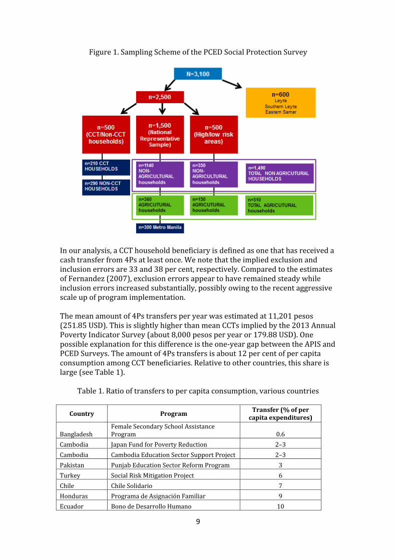
The basic variables used to generate the matched samples are the observable characteristics used for the proxy means test. We generated alternative propensity scores by augmenting the proxy means test covariates with provincial dummies to account for differences in participation level and timing. To assess the validity of the matching, we used the mean bias and pseudo R-squared1 for each comparison (as suggested in Caliendo and Kopeinig, 2008). Propensity scores were first generated for the entire sample, then CCT eligible families were defined as those with pregnant women or children below 14 years old. Matched samples were then identified following the definitions for 𝑇1-𝑇3 and 𝐶1-𝐶2. To compute the ATT, we employed kernel matching with bandwidth 0.03. Our results are consistent with alternative matching algorithms: kernel matching with bandwidth 0.05, radius matching with caliper sizes 0.01, 0.02 and 0.03. We present the results of these alternative matching algorithms in the Appendix. The fixed bandwidth and caliper sizes ensure that the matched control units have very close propensity scores to the treatment unit. Whereas radius matching treats all comparison units equally, in contrast, kernel matching attaches greater weights to those comparison units closest to the treatment unit. V. Data, Variable Definition, and Descriptive Statistics The PCED Social Protection Survey had a total sample size of 3,100 households, consisting of a nationally representative sample of 1,500 households augmented by 3 sub-samples that were drawn to facilitate analysis on various social protection research questions. We oversampled 500 households consisting of both CCT and non-CCT household beneficiaries, 500 households consisting of households residing in areas that are high- and low-risk for natural disasters such as typhoons and earthquakes, and 600 households from Leyte, Southern Leyte, and Eastern Samar which were the provinces that were most affected by the typhoon Haiyan in November 2013. From this full sample, we obtained 609 CCT household beneficiaries - 196 from the nationally representative sample, 210 from the CCT/non-CCT sub-sample, 102 from the high/low-risk sub-sample, and 101 from the Haiyan sub-sample. For this analysis, sampling weights had to be constructed so that each CCT household beneficiary reflects is true weight relative to the population. Figure 1 illustrates the sampling scheme.
1 A low R-squared (near zero) is desired. This indicates that after controlling for observable covariates, the logit model very little of variation in treatment assignment, which is what happens when the assignment is truly random.
9
Figure 1. Sampling Scheme of the PCED Social Protection Survey
In our analysis, a CCT household beneficiary is defined as one that has received a cash transfer from 4Ps at least once. We note that the implied exclusion and inclusion errors are 33 and 38 per cent, respectively. Compared to the estimates of Fernandez (2007), exclusion errors appear to have remained steady while inclusion errors increased substantially, possibly owing to the recent aggressive scale up of program implementation. The mean amount of 4Ps transfers per year was estimated at 11,201 pesos (251.85 USD). This is slightly higher than mean CCTs implied by the 2013 Annual Poverty Indicator Survey (about 8,000 pesos per year or 179.88 USD). One possible explanation for this difference is the one-year gap between the APIS and PCED Surveys. The amount of 4Ps transfers is about 12 per cent of per capita consumption among CCT beneficiaries. Relative to other countries, this share is large (see Table 1).
Table 1. Ratio of transfers to per capita consumption, various countries
Country Program Transfer (% of per capita expenditures)
Bangladesh Female Secondary School Assistance Program 0.6
Cambodia Japan Fund for Poverty Reduction 2–3 Cambodia Cambodia Education Sector Support Project 2–3 Pakistan Punjab Education Sector Reform Program 3 Turkey Social Risk Mitigation Project 6 Chile Chile Solidario 7 Honduras Programa de Asignación Familiar 9 Ecuador Bono de Desarrollo Humano 10
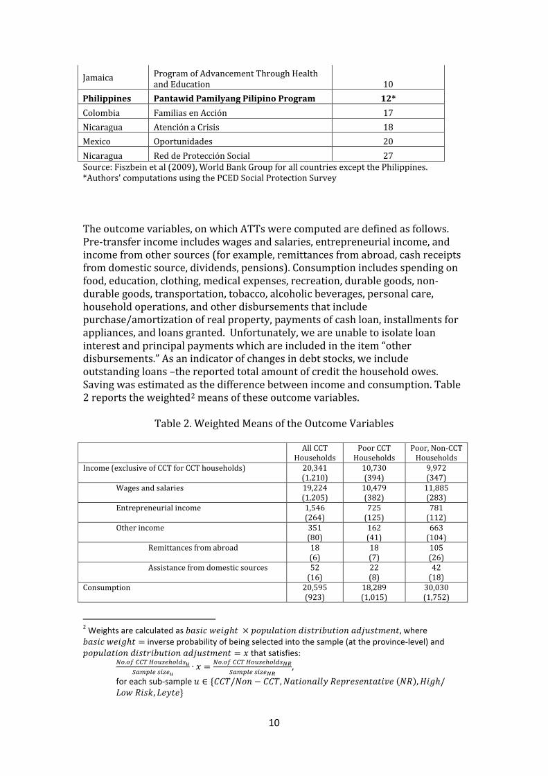
10
Jamaica Program of Advancement Through Health and Education 10
Philippines Pantawid Pamilyang Pilipino Program 12* Colombia Familias en Acción 17 Nicaragua Atención a Crisis 18 Mexico Oportunidades 20 Nicaragua Red de Protección Social 27 Source: Fiszbein et al (2009), World Bank Group for all countries except the Philippines. *Authors' computations using the PCED Social Protection Survey
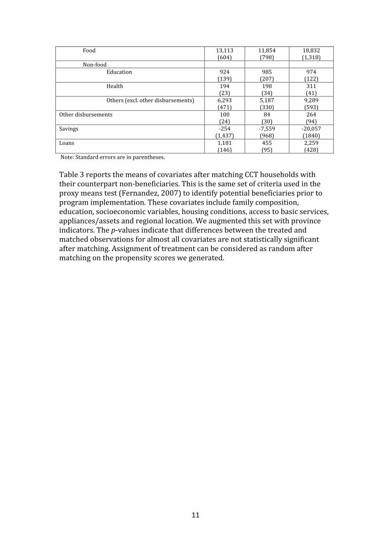
The outcome variables, on which ATTs were computed are defined as follows. Pre-transfer income includes wages and salaries, entrepreneurial income, and income from other sources (for example, remittances from abroad, cash receipts from domestic source, dividends, pensions). Consumption includes spending on food, education, clothing, medical expenses, recreation, durable goods, non-durable goods, transportation, tobacco, alcoholic beverages, personal care, household operations, and other disbursements that include purchase/amortization of real property, payments of cash loan, installments for appliances, and loans granted. Unfortunately, we are unable to isolate loan interest and principal payments which are included in the item “other disbursements.” As an indicator of changes in debt stocks, we include outstanding loans –the reported total amount of credit the household owes. Saving was estimated as the difference between income and consumption. Table 2 reports the weighted2 means of these outcome variables.
Table 2. Weighted Means of the Outcome Variables All CCT
Households Poor CCT
Households Poor, Non-CCT
Households Income (exclusive of CCT for CCT households) 20,341
(1,210) 10,730 (394)
9,972 (347)
Wages and salaries 19,224 (1,205)
10,479 (382)
11,885 (283)
Entrepreneurial income 1,546 (264)
725 (125)
781 (112)
Other income 351 (80)
162 (41)
663 (104)
Remittances from abroad 18 (6)
18 (7)
105 (26)
Assistance from domestic sources 52 (16)
22 (8)
42 (18)
Consumption 20,595 (923)
18,289 (1,015)
30,030 (1,752)
2 Weights are calculated as 𝑏𝑏𝑏𝑏𝑏 𝑤𝑤𝑏𝑤ℎ𝑡 × 𝑝𝑝𝑝𝑝𝑝𝑏𝑡𝑏𝑝𝑝 𝑑𝑏𝑏𝑡𝑟𝑏𝑏𝑝𝑡𝑏𝑝𝑝 𝑏𝑑𝑎𝑝𝑏𝑡𝑎𝑤𝑝𝑡, where 𝑏𝑏𝑏𝑏𝑏 𝑤𝑤𝑏𝑤ℎ𝑡 = inverse probability of being selected into the sample (at the province-level) and 𝑝𝑝𝑝𝑝𝑝𝑏𝑡𝑏𝑝𝑝 𝑑𝑏𝑏𝑡𝑟𝑏𝑏𝑝𝑡𝑏𝑝𝑝 𝑏𝑑𝑎𝑝𝑏𝑡𝑎𝑤𝑝𝑡 = 𝑥 that satisfies:
𝑁𝑜.𝑜𝑜 𝐶𝐶𝐶 𝐻𝑜𝐻𝐻𝑒ℎ𝑜𝑜𝑜𝐻𝑢𝑆𝑆𝑆𝑆𝑜𝑒 𝐻𝑖𝑠𝑒𝑢
∙ 𝑥 = 𝑁𝑜.𝑜𝑜 𝐶𝐶𝐶 𝐻𝑜𝐻𝐻𝑒ℎ𝑜𝑜𝑜𝐻𝑁𝑁𝑆𝑆𝑆𝑆𝑜𝑒 𝐻𝑖𝑠𝑒𝑁𝑁
,
for each sub-sample 𝑝 ∈ {𝐶𝐶𝑇/𝑁𝑝𝑝 − 𝐶𝐶𝑇,𝑁𝑏𝑡𝑏𝑝𝑝𝑏𝑝𝑝𝑁 𝑅𝑤𝑝𝑟𝑤𝑏𝑤𝑝𝑡𝑏𝑡𝑏𝑅𝑤 (𝑁𝑅),𝐻𝑏𝑤ℎ/𝑟𝑝𝑤 𝑅𝑏𝑏𝑅, 𝑟𝑤𝑁𝑡𝑤}
11
Food 13,113 (604)
11,854 (798)
18,832 (1,318)
Non-food Education 924
(139) 985
(207) 974
(122) Health 194
(23) 198 (34)
311 (41)
Others (excl. other disbursements) 6,293 (471)
5,187 (330)
9,289 (593)
Other disbursements 100 (24)
84 (30)
264 (94)
Savings -254 (1,437)
-7,559 (968)
-20,057 (1840)
Loans 1,181 (146)
455 (95)
2,259 (428)
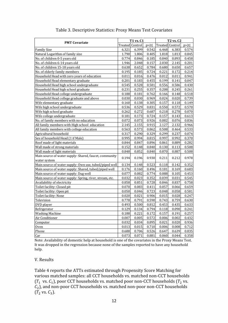
Note: Standard errors are in parentheses. Table 3 reports the means of covariates after matching CCT households with their counterpart non-beneficiaries. This is the same set of criteria used in the proxy means test (Fernandez, 2007) to identify potential beneficiaries prior to program implementation. These covariates include family composition, education, socioeconomic variables, housing conditions, access to basic services, appliances/assets and regional location. We augmented this set with province indicators. The p-values indicate that differences between the treated and matched observations for almost all covariates are not statistically significant after matching. Assignment of treatment can be considered as random after matching on the propensity scores we generated.
12
Table 3. Descriptive Statistics: Proxy Means Test Covariates
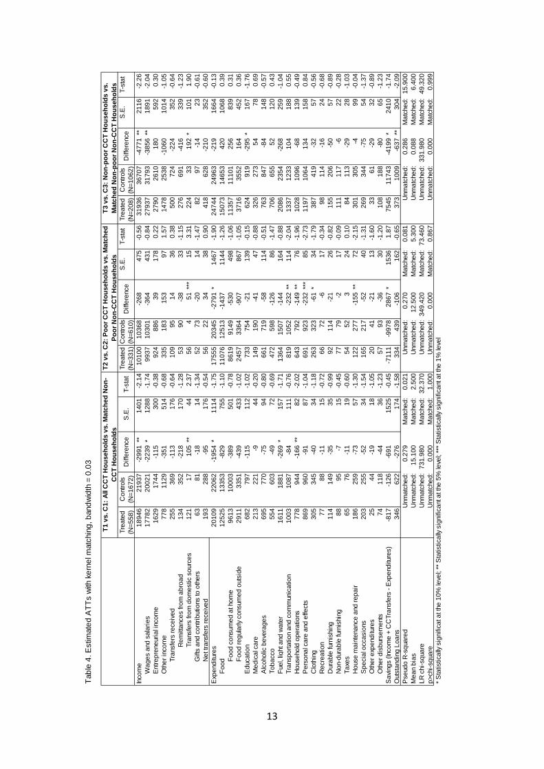
Note: Availability of domestic help at household is one of the covariates in the Proxy Means Test. It was dropped in the regression because none of the samples reported to have any household help. V. Results Table 4 reports the ATTs estimated through Propensity Score Matching for various matched samples: all CCT households vs. matched non-CCT households (𝑇1 vs. 𝐶1), poor CCT households vs. matched poor non-CCT households (𝑇2 vs. 𝐶2), and non-poor CCT households vs. matched non-poor non-CCT households (𝑇2 vs. 𝐶3).
Treated Control p>|t| Treated Control p>|t|Family Size 6.321 6.399 0.542 6.468 6.383 0.574Natural Logarithm of family size 1.790 1.806 0.405 1.818 1.813 0.845No. of children 0-5 years old 0.774 0.846 0.185 0.840 0.893 0.458No. of children 6-14 years old 1.946 2.048 0.157 2.030 2.145 0.201No. of children 15-18 years old 0.638 0.652 0.784 0.680 0.650 0.657No. of elderly family members 0.195 0.185 0.724 0.221 0.172 0.214Household Head with zero years of education 0.011 0.016 0.476 0.012 0.011 0.941Household Head elementary graduate 0.201 0.183 0.455 0.199 0.141 0.047Household Head high school undergraduate 0.545 0.528 0.581 0.556 0.586 0.430Household Head high school graduate 0.231 0.255 0.357 0.208 0.245 0.261Household Head college undergraduate 0.188 0.181 0.762 0.166 0.148 0.518Household Head college graduate and above 0.030 0.030 0.969 0.024 0.020 0.739Wife elementary graduate 0.160 0.138 0.305 0.157 0.118 0.149Wife high school undergraduate 0.536 0.529 0.831 0.550 0.572 0.570Wife high school graduate 0.262 0.272 0.687 0.218 0.278 0.070Wife college undergraduate 0.181 0.173 0.724 0.157 0.143 0.613No. of family members with no education 0.072 0.073 0.926 0.082 0.076 0.836All family members with High school education 2.145 2.155 0.915 2.127 2.132 0.966All family members with college education 0.563 0.573 0.862 0.508 0.464 0.533Agricultural household 0.317 0.290 0.329 0.299 0.237 0.074Sex of household Head (1 if Male) 0.995 0.994 0.815 0.997 0.992 0.370Roof made of light materials 0.844 0.847 0.896 0.861 0.889 0.282Wall made of strong materials 0.152 0.148 0.840 0.130 0.113 0.508Wall made of light materials 0.848 0.852 0.840 0.870 0.887 0.508
Main source of water supply: Own use, tubed/piped well 0.134 0.148 0.523 0.118 0.142 0.352Main source of water supply: Shared, tubed/piped well 0.176 0.160 0.496 0.181 0.169 0.683Main source of water supply: Dug well 0.077 0.082 0.774 0.088 0.105 0.453Main source of water supply: Spring, river, stream, etc. 0.032 0.023 0.352 0.039 0.031 0.545Availability of electricity 0.858 0.851 0.728 0.846 0.837 0.758Toilet facility: Closed pit 0.070 0.083 0.411 0.057 0.066 0.659Toilet facility: Open pit 0.050 0.046 0.723 0.048 0.058 0.581Toilet facility: None 0.020 0.021 0.906 0.015 0.028 0.247Television 0.778 0.791 0.590 0.743 0.759 0.630DVD player 0.493 0.500 0.812 0.453 0.435 0.633Refrigerator 0.129 0.134 0.794 0.118 0.090 0.241Washing Machine 0.188 0.221 0.172 0.157 0.191 0.257Air Conditioner 0.007 0.005 0.572 0.006 0.002 0.432Computer 0.032 0.034 0.895 0.021 0.020 0.936Oven 0.013 0.015 0.710 0.006 0.008 0.712Phone 0.688 0.706 0.526 0.647 0.639 0.835Car 0.073 0.071 0.881 0.060 0.044 0.358
T1 vs. C1 T2 vs. C2PMT Covariate
Main source of water supply: Shared, faucet, community water system
0.194 0.196 0.211 0.212 0.9780.930
13
Tabl
e 4.
Est
imat
ed A
TTs
with
ker
nel m
atch
ing,
ban
dwid
th =
0.0
3
Trea
ted
Con
trols
Trea
ted
Con
trols
S.E
.T-
stat
Trea
ted
Con
trols
S.E
.T-
stat
(N=5
58)
(N=1
672)
(N=3
31)
(N=6
10)
(N=2
08)
(N=1
062)
Inco
me
1894
621
937
-299
1**
1401
-2.1
410
100
1036
8-2
6847
5-0
.56
3193
636
707
-477
1**
2116
-2.2
6W
ages
and
sal
arie
s17
782
2002
1-2
239
*12
88-1
.74
9937
1030
1-3
6443
1-0
.84
2793
731
793
-385
6**
1891
-2.0
4E
ntre
pren
euria
l inc
ome
1629
1744
-115
300
-0.3
892
488
639
178
0.22
2790
2610
180
592
0.30
Oth
er in
com
e77
811
29-3
5151
4-0
.68
335
183
153
971.
5714
7825
38-1
060
1014
-1.0
5Tr
ansf
ers
rece
ived
255
369
-113
176
-0.6
410
995
1436
0.38
500
724
-224
352
-0.6
4R
emitt
ance
s fro
m a
broa
d13
435
2-2
1817
0-1
.28
5390
-38
33-1
.15
276
691
-416
339
-1.2
3Tr
ansf
ers
from
dom
estic
sou
rces
121
1710
5**
442.
3756
451
***
153.
3122
433
192
*10
11.
90G
ifts
and
cont
ribut
ions
to o
ther
s63
81-1
814
-1.3
452
73-2
014
-1.4
782
97-1
423
-0.6
1N
et tr
ansf
ers
rece
ived
193
288
-95
176
-0.5
456
2234
380.
9041
862
8-2
1035
2-0
.60
Exp
endi
ture
s20
109
2206
2-1
954
*11
14-1
.75
1755
520
345
-279
1*
1467
-1.9
024
744
2496
3-2
1916
64-0
.13
Food
1252
513
353
-829
755
-1.1
011
076
1251
3-1
437
1144
-1.2
615
073
1465
342
010
680.
39Fo
od c
onsu
med
at h
ome
9613
1000
3-3
8950
1-0
.78
8619
9149
-530
498
-1.0
611
357
1110
125
683
90.
31Fo
od re
gula
rly c
onsu
med
out
side
2911
3351
-439
433
-1.0
224
5733
64-9
0786
7-1
.05
3716
3552
164
452
0.36
Edu
catio
n68
279
7-1
1511
2-1
.02
733
754
-21
139
-0.1
562
491
9-2
95*
167
-1.7
6M
edic
al c
are
213
221
-944
-0.2
014
919
0-4
147
-0.8
832
627
354
780.
69A
lcoh
olic
bev
erag
es69
577
0-7
594
-0.8
066
171
9-5
811
4-0
.51
763
847
-84
148
-0.5
7To
bacc
o55
460
3-4
972
-0.6
947
259
8-1
2686
-1.4
770
665
552
120
0.43
Fuel
, lig
ht a
nd w
ater
1611
1881
-269
*15
7-1
.71
1364
1507
-144
164
-0.8
820
8623
54-2
6825
9-1
.04
Tran
spor
tatio
n an
d co
mm
unic
atio
n10
0310
87-8
411
1-0
.76
819
1052
-232
**11
4-2
.04
1337
1233
104
188
0.55
Hou
seho
ld o
pera
tions
778
944
-166
**82
-2.0
264
379
2-1
49**
76-1
.96
1028
1096
-68
139
-0.4
9P
erso
nal c
are
and
effe
cts
869
960
-91
87-1
.04
691
923
-232
***
85-2
.73
1197
1064
134
158
0.84
Clo
thin
g30
534
5-4
034
-1.1
826
332
3-6
1*
34-1
.79
387
419
-32
57-0
.56
Rec
reat
ion
7788
-11
15-0
.72
6672
-617
-0.3
498
114
-16
24-0
.68
Dur
able
furn
ishi
ng11
414
9-3
535
-0.9
992
114
-21
26-0
.82
155
206
-50
57-0
.89
Non
-dur
able
furn
ishi
ng88
95-7
15-0
.45
7779
-217
-0.0
911
111
7-6
22-0
.28
Taxe
s65
76-1
119
-0.6
054
523
240.
1084
113
-29
28-1
.03
Hou
se m
aint
enan
ce a
nd re
pair
186
259
-73
57-1
.30
122
277
-155
**72
-2.1
530
130
5-4
99-0
.04
Spe
cial
occ
asio
ns20
325
5-5
234
-1.5
416
521
7-5
240
-1.3
126
934
4-7
554
-1.3
7O
ther
exp
endi
ture
s25
44-1
918
-1.0
520
41-2
113
-1.6
033
61-2
932
-0.8
9O
ther
dis
burs
emen
ts74
118
-44
36-1
.23
5793
-36
30-1
.20
108
188
-80
65-1
.23
Sav
ings
(Inc
ome
+ C
CTr
ansf
ers
- Exp
endi
ture
s)-8
17-1
26-6
9115
25-0
.45
-711
1-9
978
2867
*15
361.
8775
4511
743
-419
9*
2410
-1.7
4O
utst
andi
ng L
oans
346
622
-276
174
-1.5
833
443
9-1
0616
2-0
.65
373
1009
-637
**30
4-2
.09
Pse
udo
R-s
quar
ed0.
279
Mat
ched
:0.
021
0.27
0M
atch
ed:
0.08
10.
286
Mat
ched
:15
.900
Mea
n bi
as15
.100
Mat
ched
:2.
500
12.5
00M
atch
ed:
5.30
00.
088
Mat
ched
:6.
400
LR c
hi-s
quar
e73
1.98
0M
atch
ed:
32.3
7034
9.42
0M
atch
ed:
73.4
6033
1.98
0M
atch
ed:
49.3
20p>
chi-s
quar
e0.
000
Mat
ched
:1.
000
0.00
0M
atch
ed:
0.86
70.
000
Mat
ched
:0.
999
* Sta
tistic
ally
sign
ifica
t at t
he 1
0% le
vel;
** S
tatis
tical
ly si
gnifi
cant
at t
he 5
% le
vel;
*** S
tatis
tical
ly si
gnifi
cant
at t
he 1
% le
vel
Unm
atch
ed:
Unm
atch
ed:
Unm
atch
ed:
Unm
atch
ed:
T3 v
s. C
3: N
on-p
oor C
CT
Hou
seho
lds
vs.
Mat
ched
Non
-poo
r Non
-CC
T H
ouse
hold
s
Diff
eren
ce
T1 v
s. C
1: A
ll C
CT
Hou
seho
lds
vs. M
atch
ed N
on-
CC
T H
ouse
hold
sT2
vs.
C2:
Poo
r CC
T H
ouse
hold
s vs
. Mat
ched
Po
or N
on-C
CT
Hou
seho
lds
Unm
atch
ed:
Unm
atch
ed:
Unm
atch
ed:
Unm
atch
ed:
Unm
atch
ed:
Unm
atch
ed:
Unm
atch
ed:
Unm
atch
ed:
Diff
eren
ceS
.E.
T-st
atD
iffer
ence
14
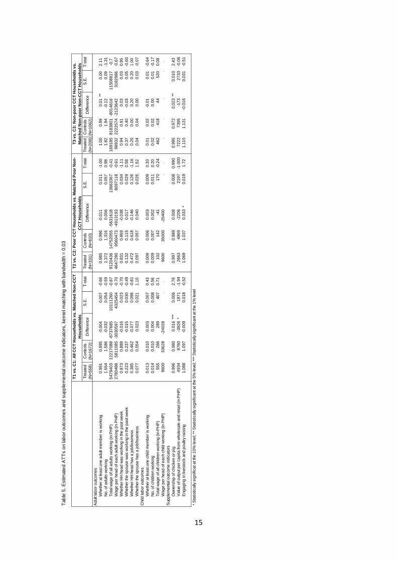
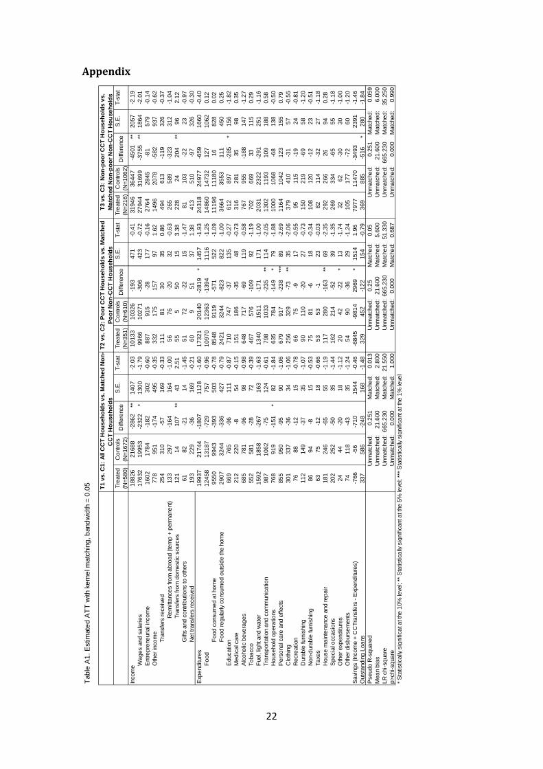
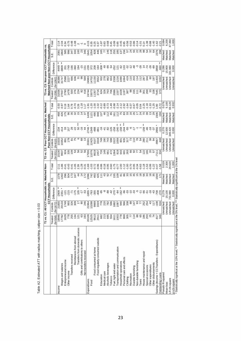
The bottom rows of Table 4 indicate match quality in terms of Pseudo R-squared, mean bias and likelihood ratio (LR). The matching algorithm we used results in nearly zero pseudo R-squared and low mean bias after matching. The LR chi-square becomes statistically significant after matching. These three statistics together indicate that the treated households are suitably matched with control households through the propensity scores we generated. 𝑇1 vs. 𝐶1, as implemented, includes both inclusion and exclusion errors. We find reduced total household income among CCT households, particularly, reduced wages and salaries. This could indicate reduced labor supply resulting from compliance with program conditions that require time, for example, participation in Family Development Sessions particularly when individual workers are paid on a piece-rate basis. This could also arise from various responses to a misperception that having continued wage employment disqualifies families from the program: actual reduction of labor supply or misreporting of actual wage income. Despite lower reported incomes for CCT households, none of the reported labor-related indicators were significantly different for CCT and non-CCT households (see Table 5). One possible explanation is the presence of disincentives for truthful revelation of work patterns, especially if there is a reduction in work effort, among program beneficiaries. We find evidence of crowding in because transfers from other domestic sources increased, suggesting possible program spillovers in the form of improved identification of the poor households for social protection programs as a whole. We also find lower spending on household operations which include laundry soap and detergent, floor wax, insect spray, etc. In 𝑇2 vs. 𝐶2, there were no significant differences in income across CCT and non-CCT households. Total transfers from all domestic sources including the 4Ps, however, are higher for 4Ps households. Total household expenditures are lower among CCT households, particularly, those that are work-related. These include transportation and communication, personal care and effects, and clothing. Thus, although we do not observe program effects on labor decisions, reduced spending in work-related items could suggest lower work effort but not truthfully reported. We also find lower spending on housing maintenance and repairs, which could be linked to program eligibility. Housing characteristics are among the PMT covariates. Arguably, if CCTs are sufficiently large, there could be disincentives to spend on housing maintenance and repairs to ensure that program eligibility is retained. Overall, given patterns in income and spending, we find lower dissaving among the poor 4P households.
15
Tabl
e 5.
Est
imat
ed A
TTs
on la
bor o
utco
mes
and
sup
plem
enta
l out
com
e in
dica
tors
, ker
nel m
atch
ing
with
ban
dwid
th =
0.0
3
Trea
ted
Con
trols
S.E
.T-
stat
Trea
ted
Con
trols
S.E
.T-
stat
Trea
ted
Con
trols
S.E
.T-
stat
(N=5
58)
(N=1
672)
(N=3
31)
(N=6
10)
(N=2
08)
(N=1
062)
Adu
lt la
bor o
utco
mes
Whe
ther
at l
east
one
adu
lt m
embe
r is
wor
king
0.99
10.
995
-0.0
040.
007
-0.6
60.
985
0.99
6-0
.011
0.01
1-1
.00
1.00
0.99
0.01
**0.
002.
11N
o. o
f adu
lts w
orki
ng1.
554
1.58
6-0
.032
0.05
4-0
.59
1.37
21.
316
0.05
60.
057
0.98
1.82
1.94
-0.1
20.
09-1
.31
Tota
l wag
e of
all a
dults
wor
king
(in
PH
P)
5479
403
1221
7088
-673
7685
1011
1260
-0.6
791
2043
614
7520
55-5
6316
1813
6633
67-0
.41
1691
8581
8380
1-8
0146
1611
5088
17-0
.7W
age
per h
ead
of e
ach
adul
t wor
king
(in
PH
P)
2780
488
5811
085
-303
0597
4325
454
-0.7
046
4728
095
6047
3-4
9131
9380
9711
8-0
.61
9893
222
2257
4-2
1236
4231
8298
6-0
.67
Whe
ther
HH
hea
d w
as w
orki
ng in
the
past
wee
k0.
873
0.88
8-0
.016
0.02
3-0
.70
0.83
10.
869
-0.0
380.
034
-1.1
10.
940.
910.
030.
030.
95W
heth
er th
e sp
ouse
was
wor
king
in th
e pa
st w
eek
0.22
30.
237
-0.0
150.
030
-0.4
90.
132
0.11
50.
017
0.02
90.
580.
370.
40-0
.03
0.05
-0.6
0W
heth
er H
H h
ead
has
a jo
b/bu
sine
ss0.
385
0.46
2-0
.077
0.09
6-0
.81
0.47
20.
618
-0.1
460.
126
-1.1
60.
200.
000.
200.
201.
00W
heth
er th
e sp
ouse
has
a jo
b/bu
sine
ss0.
077
0.05
40.
023
0.02
11.
100.
097
0.05
70.
040
0.02
61.
520.
040.
040.
000.
03-0
.07
Chi
ld la
bor o
utco
mes
Whe
ther
at l
east
one
chi
ld m
embe
r is
wor
king
0.01
30.
010
0.00
30.
007
0.43
0.00
90.
006
0.00
30.
009
0.33
0.01
0.02
-0.0
10.
01-0
.64
No.
of c
hild
ren
wor
king
0.01
40.
010
0.00
40.
008
0.56
0.00
90.
007
0.00
20.
011
0.20
0.02
0.02
0.00
0.01
-0.1
7To
tal w
age
of a
ll chi
ldre
n w
orki
ng (i
n P
HP
)55
526
628
940
70.
7110
214
2-4
117
0-0
.24
462
418
4452
00.
08W
age
per h
ead
of e
ach
child
wor
king
(in
PH
P)
9600
3362
8-2
4028
..
9600
3500
0-2
5400
..
..
..
.S
uppl
emen
tal o
utco
me
indi
cato
rsO
wne
rshi
p of
chi
cken
or p
ig0.
996
0.98
00.
016
***
0.00
62.
760.
997
0.98
90.
008
0.00
80.
990
0.99
50.
972
0.02
3**
0.01
02.
43V
alue
of o
utpu
t per
cap
ita fr
om w
hole
sale
and
reta
il (in
PH
P)
4934
8760
-382
6*
1971
-1.9
426
6348
69-2
206
2197
-1.0
0072
2273
95-1
7327
33-0
.06
Eng
agin
g in
live
stoc
k an
d po
ultry
rais
ing
1.08
81.
097
-0.0
090.
018
-0.5
21.
069
1.03
70.
033
*0.
019
1.72
1.11
51.
131
-0.0
160.
031
-0.5
1
* Sta
tistic
ally
sign
ifica
t at t
he 1
0% le
vel;
** S
tatis
tical
ly si
gnifi
cant
at t
he 5
% le
vel;
*** S
tatis
tical
ly si
gnifi
cant
at t
he 1
% le
vel
T3 v
s. C
3: N
on-p
oor C
CT
Hou
seho
lds
vs.
Mat
ched
Non
-poo
r Non
-CC
T H
ouse
hold
sT1
vs.
C1:
All
CC
T H
ouse
hold
s vs
. Mat
ched
Non
-CC
T H
ouse
hold
sT2
vs.
C2:
Poo
r CC
T H
ouse
hold
s vs
. Mat
ched
Poo
r Non
-C
CT
Hou
seho
lds
Diff
eren
ceD
iffer
ence
Diff
eren
ce
16
𝑇3 vs. 𝐶3 shows differences in outcome indicators for the non-poor households included in 4Ps versus their counterparts who were correctly excluded from the program. Our PSM estimates suggest possible adverse responses to CCTs - reduced wage income and reduced education spending. This could indicate strategic behavior on the part of the non- or near-poor who were included in the 4Ps by "mistake." Again, they could be underreporting incomes thinking that such information could lead to their eventual disqualification in the program. Another possibility is that they actually reduce work effort, to prolong their stay in the program. The desire to protect program eligibility could also manifest itself in reduced education spending. Although the survey data do not provide detailed information on education spending, one possible explanation is that CCT households transfer their children from private to public schools. Overall, total transfers from all domestic sources are larger for the non-poor 4Ps households, which magnifies the implications of the inclusion errors of the 4Ps. These households could be obtaining additional benefits from other social protection programs and transfer mechanisms after having been inadvertently tagged as "poor." There seems to be some gains in terms of consumption smoothing for this sub-group. They have lower outstanding loans and dissaving. The last three rows of Table 5 show some supplemental outcome indicators to support the apparent trends from Table 4. The observed reduction in income among 𝑇1 versus 𝐶1 could also be due to reduced entrepreneurial income, particularly, income from wholesale and retail trade. This is to be expected given that the 4Ps seems to have increased school enrollment and reduced the number of days spent in child labor (DSWD, 2014). The 2011 Survey of Children shows that next to farms, streets and markets are the most likely workplaces of children in hazardous occupations. One possible outcome of 4Ps which may not be captured in reported income and expenditures as well as computed saving is the increased investment in livestock (that is, chickens and pigs). We find that CCT households have more livestock compared to their matched controls. Among the poor, the CCT households are more likely to report being engaged in livestock and poultry raising. These patterns in livestock could suggest a smoother consumption. The ability to sustain livestock is correlated with more regular food consumption, for example, as shown in Todd et al. (2009). Finally, we conducted a sensitivity analysis using Rosenbaum bounds to see whether our findings are robust to possible confoundedness of unobserved factors. For the 𝑇1-𝐶1 comparison, our findings of reduced income and lower wages still hold even if hidden bias leads to selection bias by 75 per cent. The finding of higher transfers from other domestic sources does not remain if unobserved factors lead to selection bias. Lower total expenditure is a robust finding even if hidden bias leads to selection bias by 45 per cent. Lower spending on household operations remains robust even in the presence of selection bias of up to 90 per cent.
17
For the 𝑇2- 𝐶2 comparison, higher transfers from domestic sources remains a robust finding even if unobserved factors may lead to selection bias by 90 per cent. Lower total expenditures still holds even if hidden bias leads to selection bias by 45 per cent. The findings of lower work-related expenses are robust even in the presence of possible selection bias: up to 90 per cent for transportation and communication, up to 110 per cent for personal care and effects, and up to 55 per cent for clothing. The findings for strategic behavior on household characteristics also remain even in the presence of possible selection bias: up to 85 per cent for household operations and up to 150 per cent for house maintenance and repair. Lower dissavings among the poor CCT beneficiaries still remain even if hidden bias leads to selection bias by 40 per cent. For the 𝑇3 - 𝐶3 comparison, our findings of lower income still hold even if actual CCT households are less likely to be selected into the program by 65 per cent. Lower wages and salaries remains a robust finding up to a possible selection bias of 90 per cent. Our finding of lower spending on education still holds even if hidden bias leads to selection bias by 100 per cent. The finding on transfers from other domestic sources is not robust in the presence of unobserved confounding factors that lead to selection bias. The finding of lower dissavings still holds even in the presence of possible selection bias by 30 per cent. Lower outstanding loans is a robust finding even if actual CCT recipients are 2.5 times less likely to be selected into CCT than non-beneficiaries. However, Results of this sensitivity analysis are summarised in the Appendix (Table A5). VII. Conclusion Our analysis uses data from a special, nationally representative survey and exploits the variations arising from program inclusion and exclusion errors. Our estimates suggest profound behavioral effects from the 4Ps. CCT households - whether poor or non-poor - had increased total transfers from other domestic sources. This indicates crowding in of transfers from other sources by virtue of being CCT beneficiaries. This implies that one spillover of the 4Ps is the improved targeting of the poor for social protection programs in general. However, overall, the non-poor have higher total transfers compared to the poor. Thus, such targeting spillover seems to magnify the inclusion error of the 4Ps. It appears that as a result of increased total transfers, both the poor and non-poor, have smoother consumption over time, whether measured directly as saving or through alternative indicators such as livestock. The poor appear to have less dissaving, while the non-poor who got included in the program are less indebted. Although the reported incomes and labor decisions of the poor do not seem to be affected by the program, a number of expenditure patterns could suggest lower work effort. The poor program beneficiaries have reported lower spending on
18
transportation, personal care and effects, and clothing, all of which are work-related spending. Our study suggests possible strategic behavior among non-poor households to prolong program eligibility by reporting lower incomes. They also have reduced spending on education. One possible explanation is that children of non-poor households could be transferring from private to public schools, in order to increase compliance to the condition of continued school enrollment. Among poor households, the observed reduced spending on house maintenance and repairs could be a strategic attempt at keeping program eligibility, given that housing characteristics are PMT covariates. Further research is needed to better understand the wide range of complex behavioral responses to cash transfers. These could have important implications on the cost-effectiveness of the 4Ps.
19
References Angelucci M. and de Giorgi, G. (2009) Indirect effects of an aid programme: how
do cash transfers affect ineligibles' consumption? American Economic Review 99(1): 486–508.
Angelucci, M., Attanasio, O., and Di Maro, V. (2012) The Impact of Oportunidades
on Consumption, Savings, and Transfers*. Fiscal Studies, 33(3), 305-334. Attanasio, O. and Mesnard, A. (2006) The Impact of a Conditional Cash Transfer
Programme on Consumption in Colombia*. Fiscal Studies, 27(4), 421-442. Behrman, J., Parker S., and Todd, P. (2005) Long-term impacts of the
Oportunidades conditional cash transfer programme on rural youth in Mexico. Discussion paper, No. 122, Ibero-America Institute for Economic Research.
Borraz, F. and González, N. (2009) Impact of the Uruguayan conditional cash
transfer programme. Cuadernos de Economía (Latin American Journal of Economics), 46(134), 243–271.
Caliendo, M. and Kopeinig, S. (2008) Some practical guidance for the
implementation of propensity score matching. Journal of Economic Surveys 22(1), 31-72.
Chakraborty, S. (2013) Philippines’ Government Sponsored Health Coverage
Program for Poor Households. UNICO Studies Series 22, World Bank, Washington DC.
Chaudhury, N., Friedman, J., and Onishi, J. (2013) Philippines Conditional Cash
Transfer Program: Impact Evaluation 2012. Report Number 75533-PH, World Bank.
Del Carpio, X. and Macours, K. (2009) Leveling the intra-household playing field:
compensation and specialization in child labor allocation. Policy Research Working Paper 4822, World Bank.
de Oliveira, A. (2005) An evaluation of the Bolsa Familia programme in Brazil:
expenditures, education and labor outcomes. CEDEPLAR Working Paper. Department of Social Welfare and Development - DSWD (2014) Keeping children
healthy and in school. Evaluating the Pantawid Pamilya Using Regression Discontinuity Design. Second Wave Impact Evaluation Results. Retrieved from http://www.dswd.gov.ph/download/pantawid_pamilya_impact_evaluation/Pantawid%20Pamilya%20Impact%20Evaluation%202014%20Report%20Final.pdf
20
Fernald, L., Gertler, P., and Neufeld, L. (2009) 10-year effect of Oportunidades, Mexico's conditional cash transfer programme, on child growth, cognition, language, and behaviour: a longitudinal follow-up study. The Lancet, 374 (9706), 1997-2005.
Fernandez, L. (2007) Technical note on estimation of a proxy means test model
(PMT) for conditional cash transfer (CCT) pilot program in the Philippines. Prepared for the Department of Social Welfare and Development.
Fiszbein, A., Schady, N., and Ferreira, F. (2009) Conditional cash transfers:
reducing present and future poverty. World Bank, Washington DC. Foguel, M. and Barros, R. (2008) The effects of conditional cash transfer
programmes on adult labour supply: an empirical analysis using a time-series-cross-section sample of Brazilian municipalities. Paper presented at XXXVII Encontro Nacional De Economia, Foz do Iguaçu, Brazil.
Gertler, P. (2004) Do conditional cash transfers improve child health? Evidence
from PROGRESA's control randomized experiment. American Economic Review, 94(2), 336-341.
Gertler, P., Martinez, S., and Rubio-Codina, M. (2006) Investing cash transfers to
raise long-term living standards. Working paper series, No. 3994, Policy research, World Bank.
Hernandez, E., Sam, A., González-Vega, C., and Chen, J. (2009) Impact of
conditional cash transfers and remittances on credit market outcomes in rural Nicaragua. Presented at the Agricultural and Applied Economics Association 2009 AAEA & ACCI Joint Annual Meeting, Wisconsin.
Lagarde, M., Haines, A., and Palmer, N. (2009) The impact of conditional cash
transfers on health outcomes and use of health services in low and middle income countries. Cochrane Database Syst Rev, 4.
Orbeta, A. and Paqueo, V. (2013). Does Pantawid Foster Dependence or
Encourage Work? Evidence from a Randomized Experiments. Philippine Institute for Development Studies, Makati City.
Reyes, C. (2013) Strengthening Social Protection in the Philippines: Moving from
conditional cash transfers to universal coverage. (Draft) National Report Philippines.
Reyes, C., Tabuga, A., Mina, C., and Asis, R. (2013) Promoting Inclusive Growth
through the 4Ps. Discussion Paper Series, No. 2013-09, Philippine Institute for Development Studies.
21
Rubalcava, L., Teruel, G., and Thomas, D. (2009) Investments, time preferences, and public transfers paid to women. Economic Development and Cultural Change 57: 507–538.
Schultz, P. (2004) School subsidies for the poor: evaluating the Mexican Progresa
poverty programme. Journal of Development Economics 74: 199–250. Skoufias, E. and di Maro, V. (2008) Conditional cash transfers, adult work
incentives, and poverty. Journal of Development Studies 44: 935–960. Skoufias, E. and Parker, S. (2001) Conditional cash transfers and their impact on
child work and schooling: evidence from the Progresa programme in Mexico. Economia 2(1): 45–96.
Tavares, P. (2010) Efeito do programa Bolsa Família sobre a oferta de trabalho
dasmães. Economia e Sociedade, Campinas, vol. 19, No.3, pp.613-635. Teixeira, C. (2010) A heterogeneity analysis of the Bolsa Família programme:
effect on men and women’s work supply. Working Paper, No. 61, March 2010, International Policy Centre for Inclusive Growth – UNDP.
Todd, J., Winters, P., and Hertz, T. (2010) Conditional cash transfers and
agricultural production: lessons from the Oportunidades experience in Mexico. Journal of Development Studies, 46(1), 39-67.
Tutor, M. (2014) The impact of Philippines’ conditional cash transfer program on
consumption. Philippine Review of Economics 51(1): 117-161.
22
Appendix
Tabl
e A
1. E
stim
ated
ATT
with
ker
nel m
atch
ing,
ban
dwid
th =
0.0
5 Trea
ted
Con
trols
S.E
.T-
stat
Trea
ted
Con
trols
S.E
.T-
stat
Trea
ted
Con
trols
S.E
.T-
stat
(N=5
80)
(N=1
672)
(N=3
51)
(N=6
10)
(N=2
16)
(N=1
062)
Inco
me
1882
621
688
-286
2**
1407
-2.0
310
133
1032
6-1
9347
1-0
.41
3194
636
447
-450
1**
2057
-2.1
9W
ages
and
sal
arie
s17
632
1995
3-2
322
*13
00-1
.79
9966
1027
1-3
0642
3-0
.72
2794
431
699
-375
5**
1864
-2.0
1E
ntre
pren
euria
l inc
ome
1602
1784
-182
302
-0.6
088
791
5-2
817
7-0
.16
2764
2845
-81
579
-0.1
4O
ther
inco
me
778
951
-174
495
-0.3
533
217
515
797
1.62
1496
2078
-582
937
-0.6
2Tr
ansf
ers
rece
ived
254
310
-57
169
-0.3
311
181
3035
0.86
494
613
-119
326
-0.3
7R
emitt
ance
s fro
m a
broa
d (te
mp
+ pe
rman
ent)
133
297
-164
164
-1.0
056
76-2
032
-0.6
326
558
9-3
2331
2-1
.04
Tran
sfer
s fro
m d
omes
tic s
ourc
es12
114
107
**43
2.51
555
5015
3.38
228
2420
4**
962.
12G
ifts
and
cont
ribut
ions
to o
ther
s61
82-2
114
-1.4
551
72-2
215
-1.4
781
103
-22
23-0
.97
Net
tran
sfer
s re
ceiv
ed19
322
9-3
616
9-0
.21
609
5137
1.38
413
510
-97
326
-0.3
0E
xpen
ditu
res
1993
721
744
-180
711
28-1
.60
1732
120
140
-281
9*
1457
-1.9
324
318
2497
7-6
5916
60-0
.40
Food
1245
813
187
-729
757
-0.9
610
970
1236
3-1
394
1116
-1.2
514
860
1473
212
710
620.
12Fo
od c
onsu
med
at h
ome
9550
9943
-393
503
-0.7
885
4891
19-5
7152
2-1
.09
1119
611
180
1682
80.
02Fo
od re
gula
rly c
onsu
med
out
side
the
hom
e29
0732
44-3
3642
7-0
.79
2421
3244
-823
822
-1.0
036
6435
5311
145
00.
25E
duca
tion
669
765
-96
111
-0.8
771
074
7-3
713
5-0
.27
612
897
-285
*15
6-1
.82
Med
ical
car
e21
222
0-8
54-0
.15
151
186
-35
48-0
.73
316
281
3598
0.35
Alc
ohol
ic b
ever
ages
685
781
-96
98-0
.98
648
717
-69
119
-0.5
876
795
5-1
8814
7-1
.27
Toba
cco
552
581
-28
72-0
.39
467
576
-109
92-1
.19
702
669
3311
50.
29Fu
el, l
ight
and
wat
er15
9218
58-2
6716
3-1
.63
1340
1511
-171
171
-1.0
020
3123
22-2
9125
1-1
.16
Tran
spor
tatio
n an
d co
mm
unic
atio
n98
710
62-7
512
4-0
.61
798
1033
-235
**11
4-2
.05
1302
1193
109
188
0.58
Hou
seho
ld o
pera
tions
768
919
-151
*82
-1.8
463
578
4-1
49*
79-1
.88
1000
1068
-68
138
-0.5
0P
erso
nal c
are
and
effe
cts
855
950
-95
90-1
.06
679
917
-238
***
89-2
.69
1164
1042
123
155
0.79
Clo
thin
g30
133
7-3
634
-1.0
625
632
9-7
3**
35-2
.06
379
410
-31
57-0
.55
Rec
reat
ion
7688
-12
15-0
.78
6675
-917
-0.5
595
115
-19
24-0
.81
Dur
able
furn
ishi
ng11
214
9-3
735
-1.0
790
110
-20
27-0
.73
150
219
-69
58-1
.20
Non
-dur
able
furn
ishi
ng86
94-8
15-0
.53
7581
-618
-0.3
410
812
0-1
223
-0.5
1Ta
xes
6375
-12
18-0
.66
5353
-123
-0.0
382
114
-32
27-1
.18
Hou
se m
aint
enan
ce a
nd re
pair
181
246
-65
55-1
.19
117
280
-163
**69
-2.3
529
226
626
940.
28S
peci
al o
ccas
ions
202
252
-50
35-1
.44
162
214
-52
39-1
.35
269
334
-65
55-1
.18
Oth
er e
xpen
ditu
res
2444
-20
18-1
.12
2042
-22
*13
-1.7
432
62-3
030
-1.0
0O
ther
dis
burs
emen
ts74
118
-43
35-1
.24
5490
-36
29-1
.24
105
177
-72
60-1
.20
Sav
ings
(Inc
ome
+ C
CTr
ansf
ers
- Exp
endi
ture
s)-7
66-5
6-7
1015
44-0
.46
-684
5-9
814
2969
*15
141.
9679
7711
470
-349
323
91-1
.46
Out
stan
ding
Loa
ns33
758
6-2
4816
8-1
.48
329
452
-122
154
-0.7
936
988
5-5
16*
280
-1.8
4P
seud
o R
-squ
ared
0.25
1M
atch
ed:
0.01
30.
25M
atch
ed:
0.05
0.25
1M
atch
ed:
0.05
9M
ean
bias
21.6
00M
atch
ed:
2.80
021
.600
Mat
ched
:5.
600
21.6
00M
atch
ed:
6.00
0LR
chi
-squ
are
665.
230
Mat
ched
:21
.550
665.
230
Mat
ched
:51
.330
665.
230
Mat
ched
:35
.250
p>ch
i-squ
are
0.00
0M
atch
ed:
1.00
00.
000
Mat
ched
:0.
687
0.00
0M
atch
ed:
0.99
0* S
tatis
tical
ly si
gnifi
cat a
t the
10%
leve
l; **
Sta
tistic
ally
sign
ifica
nt a
t the
5%
leve
l; **
* Sta
tistic
ally
sign
ifica
nt a
t the
1%
leve
l
T2 v
s. C
2: P
oor C
CT
Hou
seho
lds
vs. M
atch
ed
Poor
Non
-CC
T H
ouse
hold
sT3
vs.
C3:
Non
-poo
r CC
T H
ouse
hold
s vs
. M
atch
ed N
on-p
oor N
on-C
CT
Hou
seho
lds
Unm
atch
ed:
Unm
atch
ed:
Unm
atch
ed:
Diff
eren
ceD
iffer
ence
Unm
atch
ed:
Unm
atch
ed:
Unm
atch
ed:
Unm
atch
ed:
Unm
atch
ed:
T1 v
s. C
1: A
ll C
CT
Hou
seho
lds
vs. M
atch
ed N
on-
CC
T H
ouse
hold
s
Unm
atch
ed:
Unm
atch
ed:
Unm
atch
ed:
Unm
atch
ed:
Diff
eren
ce
23
Tabl
e A
2. E
stim
ated
ATT
with
radi
us m
atch
ing,
cal
iper
siz
e =
0.03
Trea
ted
Con
trols
S.E
.T-
stat
Trea
ted
Con
trols
S.E
.T-
stat
Trea
ted
Con
trols
S.E
.T-
stat
(N=5
58)
(N=1
672)
(N=3
31)
(N=6
10)
(N=2
08)
(N=1
062)
Inco
me
1894
621
855
-290
9**
1378
-2.1
110
100
1033
3-2
3446
8-0
.50
3193
636
386
-444
9**
2081
-2.1
4W
ages
and
sal
arie
s17
782
2013
3-2
351
*12
63-1
.86
9937
1035
2-4
1442
6-0
.97
2793
731
747
-380
9**
1863
-2.0
4E
ntre
pren
euria
l inc
ome
1629
1749
-121
296
-0.4
192
489
133
175
0.19
2790
2588
201
585
0.34
Oth
er in
com
e77
899
3-2
1550
4-0
.43
335
178
157
961.
6414
7822
27-7
4999
6-0
.75
Tran
sfer
s re
ceiv
ed25
532
6-7
117
3-0
.41
109
8128
350.
7850
066
6-1
6634
7-0
.48
Rem
ittan
ces
from
abr
oad
134
309
-175
167
-1.0
553
75-2
232
-0.7
027
663
6-3
6033
3-1
.08
Tran
sfer
s fro
m d
omes
tic s
ourc
es12
117
105
**44
2.39
566
50**
*15
3.26
224
3119
410
02
Gift
s an
d co
ntrib
utio
ns to
oth
ers
6380
-17
14-1
.28
5268
-16
14-1
.18
8298
-15
23-1
Net
tran
sfer
s re
ceiv
ed19
324
6-5
317
2-0
.31
5613
4437
1.17
418
569
-151
346
0E
xpen
ditu
res
2010
921
964
-185
5*
1096
-1.6
917
555
2030
1-2
746
*14
39-1
.91
2474
424
983
-239
1641
-0.1
5Fo
od12
525
1328
8-7
6374
2-1
.03
1107
612
425
-134
911
21-1
.20
1507
314
702
372
1054
0.35
Food
con
sum
ed a
t hom
e96
1399
69-3
5549
3-0
.72
8619
9107
-488
490
-1.0
011
357
1115
020
882
80.
25Fo
od re
gula
rly c
onsu
med
out
side
2911
3319
-408
425
-0.9
624
5733
18-8
6184
8-1
.02
3716
3552
164
446
0.37
Edu
catio
n68
277
8-9
511
1-0
.86
733
749
-16
137
-0.1
262
493
2-3
08*
165
-1.8
7M
edic
al c
are
213
220
-843
-0.1
814
919
0-4
146
-0.8
932
627
849
770.
63A
lcoh
olic
bev
erag
es69
578
2-8
892
-0.9
566
174
3-8
211
2-0
.73
763
862
-99
146
-0.6
8To
bacc
o55
459
6-4
271
-0.6
047
259
8-1
2685
-1.4
970
665
354
118
0.45
Fuel
, lig
ht a
nd w
ater
1611
1882
-270
*15
5-1
.75
1364
1522
-158
161
-0.9
820
8623
38-2
5225
5-0
.99
Tran
spor
tatio
n an
d co
mm
unic
atio
n10
0310
87-8
410
9-0
.77
819
1059
-240
**11
2-2
.14
1337
1216
121
185
0.65
Hou
seho
ld o
pera
tions
778
940
-162
**81
-2.0
064
380
1-1
58**
75-2
.12
1028
1090
-62
137
-0.4
5P
erso
nal c
are
and
effe
cts
869
966
-96
86-1
.12
691
935
-244
***
83-2
.92
1197
1064
133
156
0.85
Clo
thin
g30
533
8-3
333
-1.0
026
331
7-5
533
-1.6
438
741
9-3
257
-0.5
6R
ecre
atio
n77
88-1
015
-0.7
066
73-6
16-0
.37
9811
0-1
224
-0.5
3D
urab
le fu
rnis
hing
114
147
-33
35-0
.95
9211
0-1
726
-0.6
715
520
3-4
855
-0.8
6N
on-d
urab
le fu
rnis
hing
8893
-515
-0.3
477
78-1
17-0
.05
111
114
-322
-0.1
4Ta
xes
6577
-11
18-0
.63
5454
124
0.04
8411
2-2
828
-1.0
1H
ouse
mai
nten
ance
and
repa
ir18
625
2-6
656
-1.1
812
228
0-1
58**
70-2
.25
301
287
1498
0.14
Spe
cial
occ
asio
ns20
325
4-5
133
-1.5
316
521
1-4
639
-1.1
826
934
4-7
454
-1.3
8O
ther
exp
endi
ture
s25
43-1
818
-0.9
920
38-1
813
-1.3
333
60-2
832
-0.8
8O
ther
dis
burs
emen
ts74
117
-43
35-1
.22
5794
-37
29-1
.25
108
197
-89
64-1
.40
Sav
ings
(Inc
ome
+ C
CTr
ansf
ers
- Exp
endi
ture
s)-8
17-1
08-7
0815
00-0
.47
-711
1-9
967
2856
*15
061.
9075
4511
403
-385
823
76-1
.62
Out
stan
ding
Loa
ns34
661
6-2
7017
1-1
.58
334
448
-115
159
-0.7
237
310
32-6
60**
298
-2.2
1P
seud
o R
-squ
ared
0.27
9M
atch
ed:
0.01
90.
270
Mat
ched
:0.
076
0.28
6M
atch
ed:
0.08
4M
ean
bias
15.1
00M
atch
ed:
2.30
012
.500
Mat
ched
:5.
100
15.9
00M
atch
ed:
6.20
0LR
chi
-squ
are
731.
980
Mat
ched
:29
.620
349.
420
Mat
ched
:69
.120
331.
980
Mat
ched
:47
.360
p>ch
i-squ
are
0.00
0M
atch
ed:
1.00
00.
000
Mat
ched
:0.
932
0.00
0M
atch
ed:
1.00
0* S
tatis
tical
ly si
gnifi
cat a
t the
10%
leve
l; **
Sta
tistic
ally
sign
ifica
nt a
t the
5%
leve
l; **
* Sta
tistic
ally
sign
ifica
nt a
t the
1%
leve
lU
nmat
ched
:
T1 v
s. C
1: A
ll C
CT
Hou
seho
lds
vs. M
atch
ed N
on-
CC
T H
ouse
hold
sT2
vs.
C2:
Poo
r CC
T H
ouse
hold
s vs
. Mat
ched
Po
or N
on-C
CT
Hou
seho
lds
T3 v
s. C
3: N
on-p
oor C
CT
Hou
seho
lds
vs.
Mat
ched
Non
-poo
r Non
-CC
T H
ouse
hold
s
Unm
atch
ed:
Diff
eren
ceD
iffer
ence
Diff
eren
ce
Unm
atch
ed:
Unm
atch
ed:
Unm
atch
ed:
Unm
atch
ed:
Unm
atch
ed:
Unm
atch
ed:
Unm
atch
ed:
Unm
atch
ed:
Unm
atch
ed:
Unm
atch
ed:
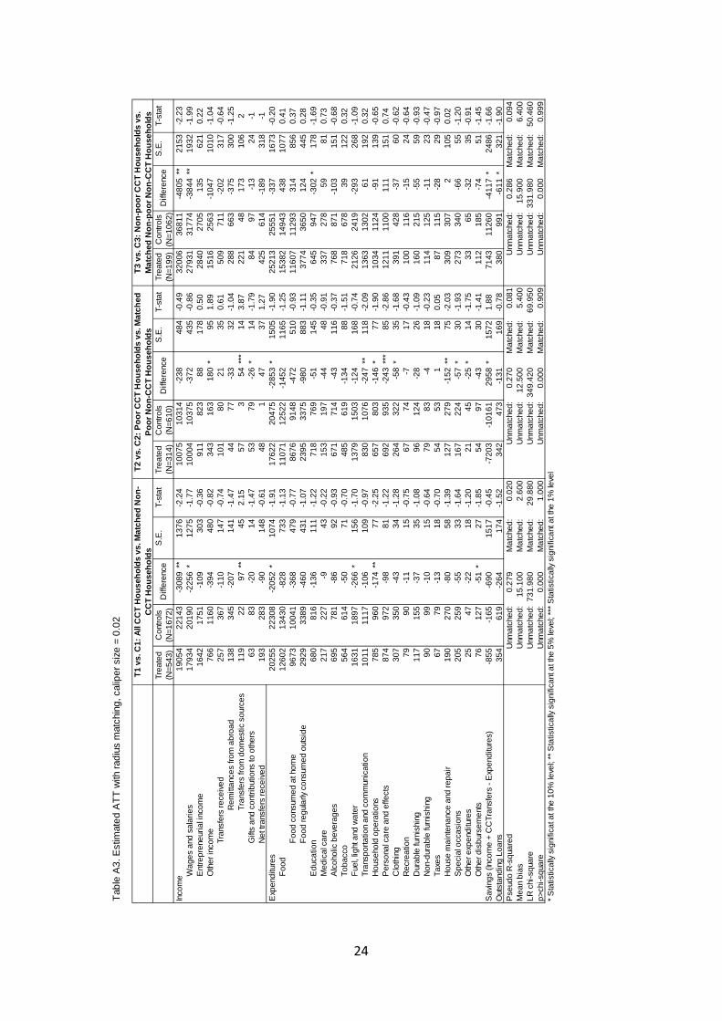
24
Tabl
e A
3. E
stim
ated
ATT
with
radi
us m
atch
ing,
cal
iper
siz
e =
0.02
Trea
ted
Con
trols
S.E
.T-
stat
Trea
ted
Con
trols
S.E
.T-
stat
Trea
ted
Con
trols
S.E
.T-
stat
(N=5
43)
(N=1
672)
(N=3
14)
(N=6
10)
(N=1
99)
(N=1
062)
Inco
me
1905
422
143
-308
9**
1376
-2.2
410
075
1031
4-2
3848
4-0
.49
3200
636
811
-480
5**
2153
-2.2
3W
ages
and
sal
arie
s17
934
2019
0-2
256
*12
75-1
.77
1000
410
375
-372
435
-0.8
627
931
3177
4-3
844
**19
32-1
.99
Ent
repr
eneu
rial i
ncom
e16
4217
51-1
0930
3-0
.36
911
823
8817
80.
5028
4027
0513
562
10.
22O
ther
inco
me
766
1160
-394
480
-0.8
234
316
318
0*
951.
8915
1625
63-1
047
1010
-1.0
4Tr
ansf
ers
rece
ived
257
367
-110
147
-0.7
410
180
2135
0.61
509
711
-202
317
-0.6
4R
emitt
ance
s fro
m a
broa
d13
834
5-2
0714
1-1
.47
4477
-33
32-1
.04
288
663
-375
300
-1.2
5Tr
ansf
ers
from
dom
estic
sou
rces
119
2297
**45
2.15
573
54**
*14
3.87
221
4817
310
62
Gift
s an
d co
ntrib
utio
ns to
oth
ers
6383
-20
14-1
.47
5379
-26
*14
-1.7
984
97-1
324
-1N
et tr
ansf
ers
rece
ived
193
283
-90
148
-0.6
148
147
371.
2742
561
4-1
8931
8-1
Exp
endi
ture
s20
255
2230
8-2
052
*10
74-1
.91
1762
220
475
-285
3*
1505
-1.9
025
213
2555
1-3
3716
73-0
.20
Food
1260
213
430
-828
733
-1.1
311
071
1252
2-1
452
1165
-1.2
515
382
1494
343
810
770.
41Fo
od c
onsu
med
at h
ome
9673
1004
1-3
6847
9-0
.77
8676
9148
-472
510
-0.9
311
607
1129
331
485
60.
37Fo
od re
gula
rly c
onsu
med
out
side
2929
3389
-460
431
-1.0
723
9533
75-9
8088
3-1
.11
3774
3650
124
445
0.28
Edu
catio
n68
081
6-1
3611
1-1
.22
718
769
-51
145
-0.3
564
594
7-3
02*
178
-1.6
9M
edic
al c
are
217
227
-943
-0.2
215
319
7-4
448
-0.9
133
727
859
810.
73A
lcoh
olic
bev
erag
es69
578
1-8
692
-0.9
367
171
4-4
311
6-0
.37
768
871
-103
151
-0.6
8To
bacc
o56
461
4-5
071
-0.7
048
561
9-1
3488
-1.5
171
867
839
122
0.32
Fuel
, lig
ht a
nd w
ater
1631
1897
-266
*15
6-1
.70
1379
1503
-124
168
-0.7
421
2624
19-2
9326
8-1
.09
Tran
spor
tatio
n an
d co
mm
unic
atio
n10
1111
17-1
0610
9-0
.97
830
1076
-247
**11
8-2
.09
1363
1302
6119
20.
32H
ouse
hold
ope
ratio
ns78
596
0-1
74**
77-2
.25
657
803
-146
*77
-1.9
010
3411
24-9
113
9-0
.65
Per
sona
l car
e an
d ef
fect
s87
497
2-9
881
-1.2
269
293
5-2
43**
*85
-2.8
612
1111
0011
115
10.
74C
loth
ing
307
350
-43
34-1
.28
264
322
-58
*35
-1.6
839
142
8-3
760
-0.6
2R
ecre
atio
n79
90-1
115
-0.7
567
74-7
17-0
.43
100
116
-15
24-0
.64
Dur
able
furn
ishi
ng11
715
5-3
735
-1.0
896
124
-28
26-1
.09
160
215
-55
59-0
.93
Non
-dur
able
furn
ishi
ng90
99-1
015
-0.6
479
83-4
18-0
.23
114
125
-11
23-0
.47
Taxe
s67
79-1
318
-0.7
054
531
180.
0587
115
-28
29-0
.97
Hou
se m
aint
enan
ce a
nd re
pair
190
270
-80
58-1
.39
127
279
-152
**75
-2.0
330
930
72
105
0.02
Spe
cial
occ
asio
ns20
525
9-5
533
-1.6
416
722
4-5
7*
30-1
.93
273
340
-66
55-1
.20
Oth
er e
xpen
ditu
res
2547
-22
18-1
.20
2145
-25
*14
-1.7
533
65-3
235
-0.9
1O
ther
dis
burs
emen
ts76
127
-51
*27
-1.8
554
97-4
330
-1.4
111
218
5-7
451
-1.4
5S
avin
gs (I
ncom
e +
CC
Tran
sfer
s - E
xpen
ditu
res)
-855
-165
-690
1517
-0.4
5-7
203
-101
6129
58*
1572
1.88
7143
1126
0-4
117
*24
86-1
.66
Out
stan
ding
Loa
ns35
461
9-2
6417
4-1
.52
342
473
-131
169
-0.7
838
099
1-6
11*
321
-1.9
0P
seud
o R
-squ
ared
0.27
9M
atch
ed:
0.02
00.
270
Mat
ched
:0.
081
0.28
6M
atch
ed:
0.09
4M
ean
bias
15.1
00M
atch
ed:
2.60
012
.500
Mat
ched
:5.
400
15.9
00M
atch
ed:
6.40
0LR
chi
-squ
are
731.
980
Mat
ched
:29
.880
349.
420
Mat
ched
:69
.950
331.
980
Mat
ched
:50
.460
p>ch
i-squ
are
0.00
0M
atch
ed:
1.00
00.
000
Mat
ched
:0.
909
0.00
0M
atch
ed:
0.99
9* S
tatis
tical
ly si
gnifi
cat a
t the
10%
leve
l; **
Sta
tistic
ally
sign
ifica
nt a
t the
5%
leve
l; **
* Sta
tistic
ally
sign
ifica
nt a
t the
1%
leve
lU
nmat
ched
:
T1 v
s. C
1: A
ll C
CT
Hou
seho
lds
vs. M
atch
ed N
on-
CC
T H
ouse
hold
sT2
vs.
C2:
Poo
r CC
T H
ouse
hold
s vs
. Mat
ched
Po
or N
on-C
CT
Hou
seho
lds
T3 v
s. C
3: N
on-p
oor C
CT
Hou
seho
lds
vs.
Mat
ched
Non
-poo
r Non
-CC
T H
ouse
hold
s
Unm
atch
ed:
Diff
eren
ceD
iffer
ence
Diff
eren
ce
Unm
atch
ed:
Unm
atch
ed:
Unm
atch
ed:
Unm
atch
ed:
Unm
atch
ed:
Unm
atch
ed:
Unm
atch
ed:
Unm
atch
ed:
Unm
atch
ed:
Unm
atch
ed:
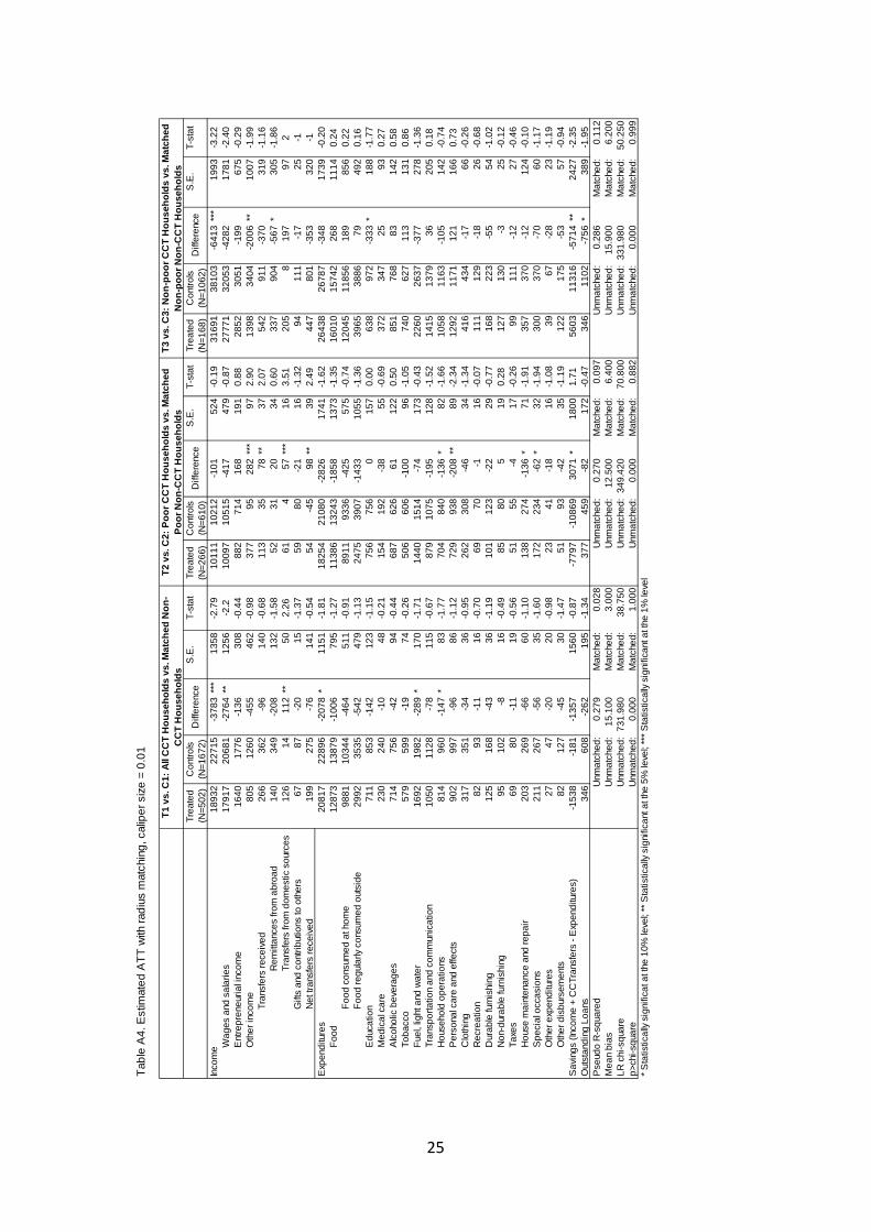
25
Tabl
e A
4. E
stim
ated
ATT
with
radi
us m
atch
ing,
cal
iper
siz
e =
0.01
Trea
ted
Con
trols
S.E
.T-
stat
Trea
ted
Con
trols
S.E
.T-
stat
Trea
ted
Con
trols
S.E
.T-
stat
(N=5
02)
(N=1
672)
(N=2
66)
(N=6
10)
(N=1
68)
(N=1
062)
Inco
me
1893
222
715
-378
3**
*13
58-2
.79
1011
110
212
-101
524
-0.1
931
691
3810
3-6
413
***
1993
-3.2
2W
ages
and
sal
arie
s17
917
2068
1-2
764
**12
56-2
.210
097
1051
5-4
1747
9-0
.87
2777
132
053
-428
217
81-2
.40
Ent
repr
eneu
rial i
ncom
e16
4017
76-1
3630
8-0
.44
882
714
168
191
0.88
2852
3051
-199
675
-0.2
9O
ther
inco
me
805
1260
-455
462
-0.9
837
795
282
***
972.
9013
9834
04-2
006
**10
07-1
.99
Tran
sfer
s re
ceiv
ed26
636
2-9
614
0-0
.68
113
3578
**37
2.07
542
911
-370
319
-1.1
6R
emitt
ance
s fro
m a
broa
d14
034
9-2
0813
2-1
.58
5231
2034
0.60
337
904
-567
*30
5-1
.86
Tran
sfer
s fro
m d
omes
tic s
ourc
es12
614
112
**50
2.26
614
57**
*16
3.51
205
819
797
2G
ifts
and
cont
ribut
ions
to o
ther
s67
87-2
015
-1.3
759
80-2
116
-1.3
294
111
-17
25-1
Net
tran
sfer
s re
ceiv
ed19
927
5-7
614
1-0
.54
54-4
598
**39
2.49
447
801
-353
320
-1E
xpen
ditu
res
2081
722
896
-207
8*
1151
-1.8
118
254
2108
0-2
826
1741
-1.6
226
438
2678
7-3
4817
39-0
.20
Food
1287
313
879
-100
679
5-1
.27
1138
613
243
-185
813
73-1
.35
1601
015
742
268
1114
0.24
Food
con
sum
ed a
t hom
e98
8110
344
-464
511
-0.9
189
1193
36-4
2557
5-0
.74
1204
511
856
189
856
0.22
Food
regu
larly
con
sum
ed o
utsi
de29
9235
35-5
4247
9-1
.13
2475
3907
-143
310
55-1
.36
3965
3886
7949
20.
16E
duca
tion
711
853
-142
123
-1.1
575
675
60
157
0.00
638
972
-333
*18
8-1
.77
Med
ical
car
e23
024
0-1
048
-0.2
115
419
2-3
855
-0.6
937
234
725
930.
27A
lcoh
olic
bev
erag
es71
475
6-4
294
-0.4
468
762
661
122
0.50
851
768
8314
20.
58To
bacc
o57
959
9-1
974
-0.2
650
660
6-1
0096
-1.0
574
062
711
313
10.
86Fu
el, l
ight
and
wat
er16
9219
82-2
89*
170
-1.7
114
4015
14-7
417
3-0
.43
2260
2637
-377
278
-1.3
6Tr
ansp
orta
tion
and
com
mun
icat
ion
1050
1128
-78
115
-0.6
787
910
75-1
9512
8-1
.52
1415
1379
3620
50.
18H
ouse
hold
ope
ratio
ns81
496
0-1
47*
83-1
.77
704
840
-136
*82
-1.6
610
5811
63-1
0514
2-0
.74
Per
sona
l car
e an
d ef
fect
s90
299
7-9
686
-1.1
272
993
8-2
08**
89-2
.34
1292
1171
121
166
0.73
Clo
thin
g31
735
1-3
436
-0.9
526
230
8-4
634
-1.3
441
643
4-1
766
-0.2
6R
ecre
atio
n82
93-1
116
-0.7
069
70-1
16-0
.07
111
129
-18
26-0
.68
Dur
able
furn
ishi
ng12
516
8-4
336
-1.1
910
112
3-2
229
-0.7
716
822
3-5
554
-1.0
2N
on-d
urab
le fu
rnis
hing
9510
2-8
16-0
.49
8580
519
0.28
127
130
-325
-0.1
2Ta
xes
6980
-11
19-0
.56
5155
-417
-0.2
699
111
-12
27-0
.46
Hou
se m
aint
enan
ce a
nd re
pair
203
269
-66
60-1
.10
138
274
-136
*71
-1.9
135
737
0-1
212
4-0
.10
Spe
cial
occ
asio
ns21
126
7-5
635
-1.6
017
223
4-6
2*
32-1
.94
300
370
-70
60-1
.17
Oth
er e
xpen
ditu
res
2747
-20
20-0
.98
2341
-18
16-1
.08
3967
-28
23-1
.19
Oth
er d
isbu
rsem
ents
8212
7-4
530
-1.4
751
93-4
235
-1.1
912
217
5-5
357
-0.9
4S
avin
gs (I
ncom
e +
CC
Tran
sfer
s - E
xpen
ditu
res)
-153
8-1
81-1
357
1560
-0.8
7-7
797
-108
6930
71*
1800
1.71
5603
1131
6-5
714
**24
27-2
.35
Out
stan
ding
Loa
ns34
660
8-2
6219
5-1
.34
377
459
-82
172
-0.4
734
611
02-7
56*
389
-1.9
5P
seud
o R
-squ
ared
0.27
9M
atch
ed:
0.02
80.
270
Mat
ched
:0.
097
0.28
6M
atch
ed:
0.11
2M
ean
bias
15.1
00M
atch
ed:
3.00
012
.500
Mat
ched
:6.
400
15.9
00M
atch
ed:
6.20
0LR
chi
-squ
are
731.
980
Mat
ched
:38
.750
349.
420
Mat
ched
:70
.800
331.
980
Mat
ched
:50
.250
p>ch
i-squ
are
0.00
0M
atch
ed:
1.00
00.
000
Mat
ched
:0.
882
0.00
0M
atch
ed:
0.99
9* S
tatis
tical
ly si
gnifi
cat a
t the
10%
leve
l; **
Sta
tistic
ally
sign
ifica
nt a
t the
5%
leve
l; **
* Sta
tistic
ally
sign
ifica
nt a
t the
1%
leve
l
Unm
atch
ed:
Unm
atch
ed:
Unm
atch
ed:
Diff
eren
ceD
iffer
ence
Unm
atch
ed:
Unm
atch
ed:
Unm
atch
ed:
T1 v
s. C
1: A
ll C
CT
Hou
seho
lds
vs. M
atch
ed N
on-
CC
T H
ouse
hold
sT2
vs.
C2:
Poo
r CC
T H
ouse
hold
s vs
. Mat
ched
Po
or N
on-C
CT
Hou
seho
lds
T3 v
s. C
3: N
on-p
oor C
CT
Hou
seho
lds
vs. M
atch
ed
Non
-poo
r Non
-CC
T H
ouse
hold
s
Unm
atch
ed:
Unm
atch
ed:
Diff
eren
ce
Unm
atch
ed:
Unm
atch
ed:
Unm
atch
ed:
Unm
atch
ed:
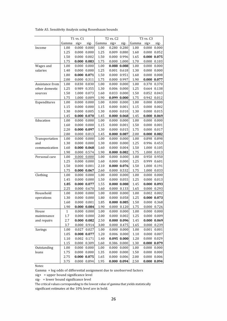
26
Table A5. Sensitivity Analysis using Rosenbaum bounds
Gamma sig+ sig- Gamma sig+ sig- Gamma sig+ sig-Income 1.00 0.000 0.000 1.00 0.280 0.280 1.00 0.000 0.000
1.25 0.000 0.000 1.25 0.009 0.880 1.60 0.000 0.0521.50 0.000 0.002 1.50 0.000 0.996 1.65 0.000 0.0751.75 0.000 0.083 1.75 0.000 1.000 1.70 0.000 0.1031.00 0.000 0.000 1.00 0.088 0.088 1.00 0.000 0.0001.40 0.000 0.000 1.25 0.001 0.618 1.30 0.000 0.0001.80 0.000 0.071 1.50 0.000 0.951 1.60 0.000 0.0082.00 0.000 0.311 1.75 0.000 0.997 1.90 0.000 0.0771.00 0.830 0.830 1.00 0.000 0.000 1.00 0.370 0.3701.25 0.989 0.355 1.30 0.006 0.000 1.25 0.664 0.1381.50 1.000 0.073 1.60 0.033 0.000 1.50 0.852 0.0431.75 1.000 0.009 1.90 0.099 0.000 1.75 0.942 0.012
Expenditures 1.00 0.000 0.000 1.00 0.000 0.000 1.00 0.000 0.0001.15 0.000 0.000 1.15 0.000 0.001 1.15 0.000 0.0021.30 0.000 0.005 1.30 0.000 0.010 1.30 0.000 0.0151.45 0.000 0.070 1.45 0.000 0.068 1.45 0.000 0.069
Education 1.00 0.000 0.000 1.00 0.000 0.000 1.00 0.000 0.0001.60 0.000 0.000 1.15 0.000 0.001 1.50 0.000 0.0012.20 0.000 0.097 1.30 0.000 0.015 1.75 0.000 0.0172.80 0.000 0.813 1.45 0.000 0.087 2.00 0.000 0.0821.00 0.000 0.000 1.00 0.000 0.000 1.00 0.898 0.8981.30 0.000 0.000 1.30 0.000 0.000 1.25 0.996 0.4531.60 0.000 0.068 1.60 0.000 0.004 1.50 1.000 0.1051.90 0.000 0.574 1.90 0.000 0.082 1.75 1.000 0.013
Personal care 1.00 0.000 0.000 1.00 0.000 0.000 1.00 0.950 0.9501.25 0.000 0.000 1.60 0.000 0.000 1.25 0.999 0.6011.50 0.000 0.001 2.10 0.000 0.076 1.50 1.000 0.1911.75 0.000 0.067 2.60 0.000 0.532 1.75 1.000 0.033
Clothing 1.00 0.000 0.000 1.00 0.000 0.000 1.00 0.000 0.0001.45 0.000 0.000 1.50 0.000 0.055 1.25 0.000 0.0131.85 0.000 0.077 1.55 0.000 0.088 1.45 0.000 0.0932.25 0.000 0.670 1.60 0.000 0.133 1.65 0.000 0.2931.00 0.000 0.000 1.00 0.000 0.000 1.00 0.002 0.0021.30 0.000 0.000 1.80 0.000 0.058 1.25 0.000 0.0731.60 0.000 0.001 1.85 0.000 0.085 1.50 0.000 0.3681.90 0.000 0.084 1.90 0.000 0.120 1.75 0.000 0.726
1 0.000 0.000 1.00 0.000 0.000 1.00 0.000 0.0001.7 0.000 0.000 2.00 0.000 0.002 1.25 0.000 0.0092.7 0.000 0.082 2.50 0.000 0.096 1.45 0.000 0.0693.7 0.000 0.914 3.00 0.000 0.475 1.65 0.000 0.239
Savings 1.00 0.027 0.027 1.00 0.000 0.000 1.00 0.001 0.0011.05 0.008 0.077 1.20 0.006 0.000 1.10 0.000 0.0071.10 0.002 0.171 1.40 0.095 0.000 1.20 0.000 0.0291.15 0.000 0.309 1.60 0.386 0.000 1.30 0.000 0.0791.00 0.000 0.000 1.00 0.000 0.000 1.00 0.000 0.0001.75 0.000 0.000 1.35 0.000 0.000 1.50 0.000 0.0002.75 0.000 0.075 1.65 0.000 0.006 2.00 0.000 0.0063.75 0.000 0.894 1.95 0.000 0.094 2.50 0.000 0.094
Notes:Gamma = log odds of differential assignment due to unobserved factorssig+ = upper bound significance levelsig- = lower bound significance levelThe critical values corresponding to the lowest value of gamma that yields statistically significant estimates at the 10% level are in bold.
House maintenance and repairs
Outstanding loans
T1 vs. C1 T2 vs. C2 T3 vs. C3
Transportation and communication
Wages and salaries
Assistance from other domestic sources
Household operations