Embed Size (px)
Citation preview

Determining User State andMental Task Demand
From Electroencephalographic Data
Diplomarbeit
Matthias Honal
University of Karlsruhe
Supervisors:Dr. Tanja Schultz
Prof. Dr. Alexander Waibel
November 2005


Ich erklare hiermit, dass ich die vorliegende Arbeit selbststandig verfasst und keine anderen als dieangegebenen Quellen und Hilfsmittel verwendet habe.
Karlsruhe, den 30.11.2005


Contents
1 Introduction 21.1 Goal . . . . . . . . . . . . . . . . . . . . . . . . . . . . . . . . . . . . . . . . . . . 21.2 Motivation . . . . . . . . . . . . . . . . . . . . . . . . . . . . . . . . . . . . . . . . 3
1.2.1 Human-Machine Interaction . . . . . . . . . . . . . . . . . . . . . . . . . . 31.2.2 Enhance Face-to-Face Communication . . . . . . . . . . . . . . . . . . . . 51.2.3 Measure Usability . . . . . . . . . . . . . . . . . . . . . . . . . . . . . . . 6
1.3 Ethical Considerations . . . . . . . . . . . . . . . . . . . . . . . . . . . . . . . . . 71.4 Contributions . . . . . . . . . . . . . . . . . . . . . . . . . . . . . . . . . . . . . . 81.5 Overview . . . . . . . . . . . . . . . . . . . . . . . . . . . . . . . . . . . . . . . . 8
2 Bio-Medical Background 102.1 Anatomy and Physiology of the Brain . . . . . . . . . . . . . . . . . . . . . . . . . 10
2.1.1 Brain Anatomy . . . . . . . . . . . . . . . . . . . . . . . . . . . . . . . . . 102.1.2 Brain physiology . . . . . . . . . . . . . . . . . . . . . . . . . . . . . . . . 12
2.2 Monitoring Brain Activity . . . . . . . . . . . . . . . . . . . . . . . . . . . . . . . 152.2.1 The Electroencephalogram (EEG) . . . . . . . . . . . . . . . . . . . . . . . 162.2.2 The Magnetoencephalogram (MEG) . . . . . . . . . . . . . . . . . . . . . . 282.2.3 Functional Near-Infrared Spectroscopy (fNIRS) . . . . . . . . . . . . . . . . 292.2.4 Functional Magnetic Resonance Imaging (fMRI) . . . . . . . . . . . . . . . 292.2.5 Single Photon Emission Computer Tomography (SPECT) . . . . . . . . . . 302.2.6 Positron Emission Tomography (PET) . . . . . . . . . . . . . . . . . . . . . 302.2.7 Summary . . . . . . . . . . . . . . . . . . . . . . . . . . . . . . . . . . . . 31
2.3 Physiological Correlates Mental States and Task Demand . . . . . . . . . . . . . . . 312.3.1 Functional Cortex Divisions and and the Identification of Mental States in the
EEG . . . . . . . . . . . . . . . . . . . . . . . . . . . . . . . . . . . . . . . 312.3.2 Task Demand, Alertness and Vigilance . . . . . . . . . . . . . . . . . . . . 35
3 Related Work 403.1 Identification of Mental States . . . . . . . . . . . . . . . . . . . . . . . . . . . . . 413.2 Assessment of Task Demand, Vigilance or Alertness . . . . . . . . . . . . . . . . . 453.3 Brain-Computer-Interfaces . . . . . . . . . . . . . . . . . . . . . . . . . . . . . . . 50
4 Methods 524.1 Artifact Removal . . . . . . . . . . . . . . . . . . . . . . . . . . . . . . . . . . . . 52
4.1.1 Removal of Eye Activity Artifacts . . . . . . . . . . . . . . . . . . . . . . . 524.1.2 Independent Component Analysis . . . . . . . . . . . . . . . . . . . . . . . 54

CONTENTS 5
4.2 Feature Extraction . . . . . . . . . . . . . . . . . . . . . . . . . . . . . . . . . . . . 584.2.1 Obtaining Feature Vectors . . . . . . . . . . . . . . . . . . . . . . . . . . . 584.2.2 Averaging . . . . . . . . . . . . . . . . . . . . . . . . . . . . . . . . . . . . 594.2.3 Normalization . . . . . . . . . . . . . . . . . . . . . . . . . . . . . . . . . 60
4.3 Feature Reduction . . . . . . . . . . . . . . . . . . . . . . . . . . . . . . . . . . . . 604.3.1 Averaging over Frequency Bands . . . . . . . . . . . . . . . . . . . . . . . 614.3.2 Linear Discriminant Analysis (LDA) . . . . . . . . . . . . . . . . . . . . . 614.3.3 Feature Reduction of Regression Tasks . . . . . . . . . . . . . . . . . . . . 624.3.4 Problems of Feature Reduction Methods . . . . . . . . . . . . . . . . . . . . 64
4.4 Self-organizing Maps (SOMs) for Data Analysis . . . . . . . . . . . . . . . . . . . . 644.4.1 Motivation . . . . . . . . . . . . . . . . . . . . . . . . . . . . . . . . . . . 644.4.2 Principle . . . . . . . . . . . . . . . . . . . . . . . . . . . . . . . . . . . . 65
4.5 Classification and Regression . . . . . . . . . . . . . . . . . . . . . . . . . . . . . . 684.5.1 Artificial Neural Networks (ANNs) . . . . . . . . . . . . . . . . . . . . . . 694.5.2 Support-Vector-Machines (SVMs) . . . . . . . . . . . . . . . . . . . . . . . 764.5.3 Multiple Linear Regression . . . . . . . . . . . . . . . . . . . . . . . . . . . 83
4.6 Performance Measurements . . . . . . . . . . . . . . . . . . . . . . . . . . . . . . . 854.6.1 Performance Measurements for Classification Problems . . . . . . . . . . . 854.6.2 Performance Measurements for Regression Problems . . . . . . . . . . . . . 87
5 Data Collection 895.1 Recording Setup . . . . . . . . . . . . . . . . . . . . . . . . . . . . . . . . . . . . . 895.2 User State Data . . . . . . . . . . . . . . . . . . . . . . . . . . . . . . . . . . . . . 905.3 Task Demand Data . . . . . . . . . . . . . . . . . . . . . . . . . . . . . . . . . . . 94
6 Experiments and Results 1006.1 User State Identification . . . . . . . . . . . . . . . . . . . . . . . . . . . . . . . . 100
6.1.1 Experimental Setups . . . . . . . . . . . . . . . . . . . . . . . . . . . . . . 1006.1.2 ANN topology selection . . . . . . . . . . . . . . . . . . . . . . . . . . . . 1016.1.3 Classifier comparison . . . . . . . . . . . . . . . . . . . . . . . . . . . . . . 1026.1.4 Averaging . . . . . . . . . . . . . . . . . . . . . . . . . . . . . . . . . . . . 1066.1.5 Normalization . . . . . . . . . . . . . . . . . . . . . . . . . . . . . . . . . 1076.1.6 Artifact Removal . . . . . . . . . . . . . . . . . . . . . . . . . . . . . . . . 1086.1.7 Feature Reduction . . . . . . . . . . . . . . . . . . . . . . . . . . . . . . . 1116.1.8 Electrode Reduction . . . . . . . . . . . . . . . . . . . . . . . . . . . . . . 1156.1.9 Analysis of Best System Configuration . . . . . . . . . . . . . . . . . . . . 1166.1.10 Prototype System . . . . . . . . . . . . . . . . . . . . . . . . . . . . . . . . 119
6.2 Assessment of Mental Task Demand . . . . . . . . . . . . . . . . . . . . . . . . . . 1206.2.1 Data Analysis using SOMs . . . . . . . . . . . . . . . . . . . . . . . . . . . 1206.2.2 Experimental Setups . . . . . . . . . . . . . . . . . . . . . . . . . . . . . . 1266.2.3 ANN topology selection . . . . . . . . . . . . . . . . . . . . . . . . . . . . 1276.2.4 Comparison of Prediction Methods . . . . . . . . . . . . . . . . . . . . . . 1276.2.5 Averaging . . . . . . . . . . . . . . . . . . . . . . . . . . . . . . . . . . . . 1336.2.6 Normalization . . . . . . . . . . . . . . . . . . . . . . . . . . . . . . . . . 1346.2.7 Feature Reduction . . . . . . . . . . . . . . . . . . . . . . . . . . . . . . . 1356.2.8 Combination of Two Subjective Task Demand Evaluations . . . . . . . . . . 1396.2.9 Electrode Reduction . . . . . . . . . . . . . . . . . . . . . . . . . . . . . . 140

CONTENTS 6
6.2.10 Analysis of Best System Configuration . . . . . . . . . . . . . . . . . . . . 141
7 Conclusions and Future Work 144

List of Figures
1.1 A typical meeting. Picture taken from [Student Government, University of Maine, 2005] 51.2 Overview of the system for user state identification and task demand estimation. . . . 9
2.1 Different anatomical parts of the human brain, with modifications from [ScientificLearning Cooperation, 1999] . . . . . . . . . . . . . . . . . . . . . . . . . . . . . . 11
2.2 Different cortex lobes, with modifications from [Scientific Learning Cooperation, 1999]. 122.3 Main components of a neuron. At the synapses information between neighboring
neurons is exchanged. In this figure the axon is myelinated as in most cases which isa mean to speed up the signal transfer. . . . . . . . . . . . . . . . . . . . . . . . . . 13
2.4 Information transfer between neurons. The thickness of the lines in the soma symbol-izes the signal amplitude. See text for explanation. . . . . . . . . . . . . . . . . . . 13
2.5 Dipole structure of cortical field potentials for a single neuron (a pyramid cell). Withmodifications from [Zschocke, 1995] . . . . . . . . . . . . . . . . . . . . . . . . . . 14
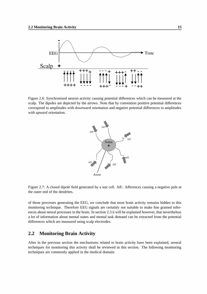
2.6 Synchronized neuron activity causing potential differences which can be measured atthe scalp. The dipoles are depicted by the arrows. Note that by convention positive po-tential differences correspond to amplitudes with downward orientation and negativepotential differences to amplitudes with upward orientation. . . . . . . . . . . . . . 15
2.7 A closed dipole field generated by a star cell. Aff.: Afferences causing a negative poleat the outer end of the dendrites. . . . . . . . . . . . . . . . . . . . . . . . . . . . . 15
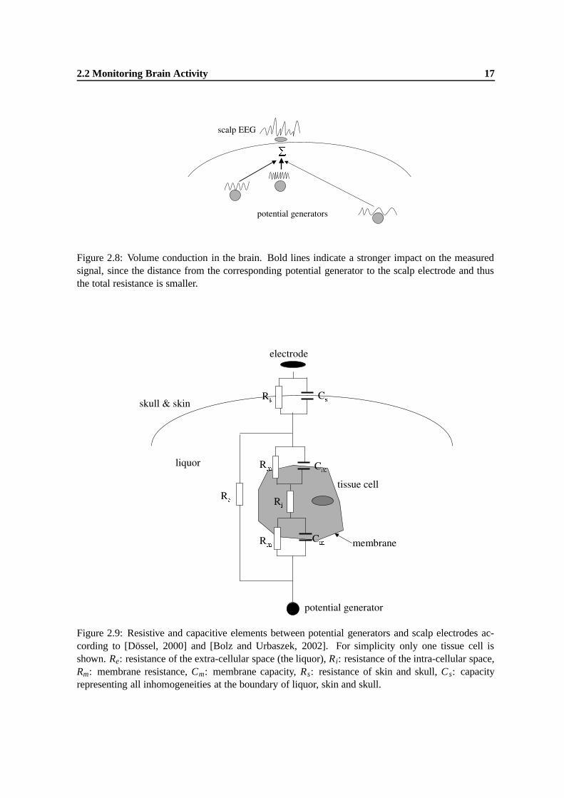
2.8 Volume conduction in the brain. Bold lines indicate a stronger impact on the measuredsignal, since the distance from the corresponding potential generator to the scalp elec-trode and thus the total resistance is smaller. . . . . . . . . . . . . . . . . . . . . . . 17
2.9 Resistive and capacitive elements between potential generators and scalp electrodesaccording to [Dossel, 2000] and [Bolz and Urbaszek, 2002]. For simplicity only onetissue cell is shown. Re: resistance of the extra-cellular space (the liquor), Ri: resis-tance of the intra-cellular space, Rm: membrane resistance, Cm: membrane capacity,Rs: resistance of skin and skull, Cs: capacity representing all inhomogeneities at theboundary of liquor, skin and skull. . . . . . . . . . . . . . . . . . . . . . . . . . . . 17
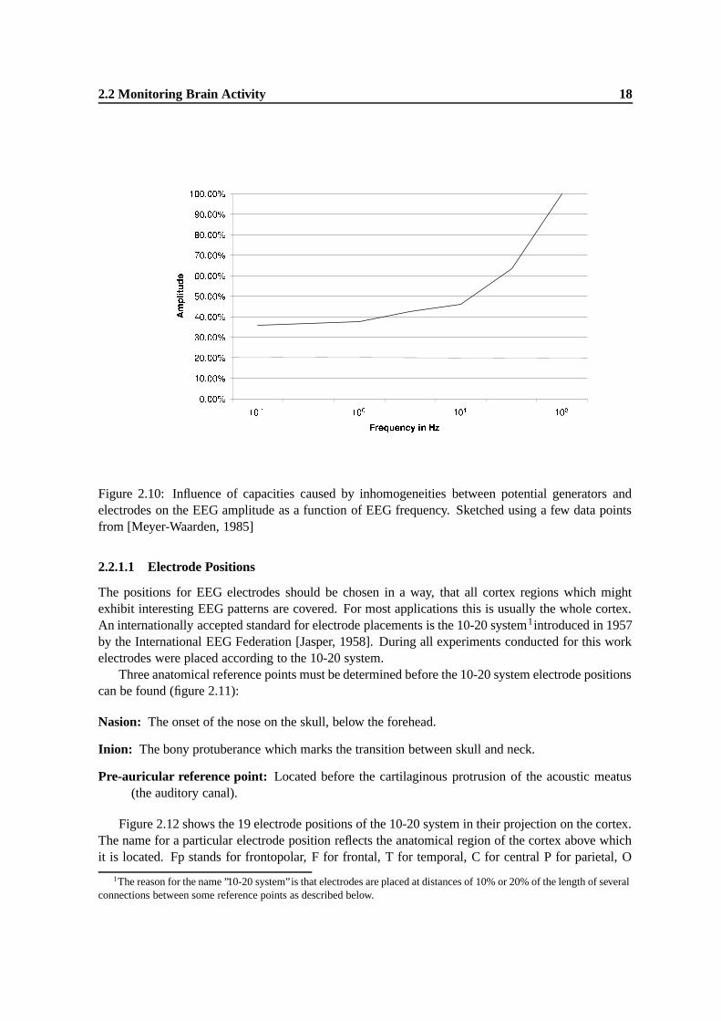
2.10 Influence of capacities caused by inhomogeneities between potential generators andelectrodes on the EEG amplitude as a function of EEG frequency. Sketched using afew data points from [Meyer-Waarden, 1985] . . . . . . . . . . . . . . . . . . . . . 18
2.11 Anatomical reference points which represent the starting points for finding the elec-trode positions defined by the 10-20 system (with modifications from [Zschocke, 1995]). 19
2.12 Electrode positions of the 10-20 system (with modifications from [Zschocke, 1995]) . 20

LIST OF FIGURES 8
2.13 The Helmholtz double layer. Since the potential of the metal ϕm is smaller than theelectrolyte potential ϕe, the hydrogen molecules of the water dipoles point the metalside. . . . . . . . . . . . . . . . . . . . . . . . . . . . . . . . . . . . . . . . . . . . 22
2.14 Electrical diagram of an electrode. Ch and R f represent the capacitive and resistiveparts of the impedance at the boundary between electrolyte and metal phase (i.e. atthe Helmholtz double layer). They vary with different frequencies. Rz is the resistanceof the electrolyte. . . . . . . . . . . . . . . . . . . . . . . . . . . . . . . . . . . . . 22
2.15 Behavior of the complex electrode impedance (the real part corresponds to the resis-tive component, the imaginary part to the capacitive component) for different currentdensities and frequencies (from [Meyer-Waarden, 1985]). . . . . . . . . . . . . . . . 23
2.16 Signal attenuation for varying frequencies for Ag/AgCl electrodes and stainless steelelectrodes with 1.0mm (SS 1.0mm) and 0.5mm (SS 0.5mm) tip size, which are usu-ally applied for intracranial recordings. With modifications from [Niedermeyer andda Silva, 1987]. . . . . . . . . . . . . . . . . . . . . . . . . . . . . . . . . . . . . . 24
2.17 Principle of non-polarized Ag/AgCl electrodes with KCl electrolyte. Left: excess ofCl− ions in the electrolyte, right: excess of K+ ions in the electrolyte. . . . . . . . . . 24
2.18 Principal of differential EEG measurement. See text for the explanation. . . . . . . . 252.19 Principle of voltage adaptation. Rs1 and Rs2 are the skin impedances, Re1 and Re2 the
electrode impedances and Rin1 and Rin2 the input impedances of the amplifier. Theaverage signal amplitude for both channels becomes approximately equal, only afterthe input impedances. . . . . . . . . . . . . . . . . . . . . . . . . . . . . . . . . . . 26
2.20 Main components of an EEG amplifier. . . . . . . . . . . . . . . . . . . . . . . . . 272.21 Generation mechanism of biological artifacts caused by large dipoles which are su-
perimposed on the EEG related dipoles. . . . . . . . . . . . . . . . . . . . . . . . . 272.22 Principal of a PET system (with modifications from [Dossel, 2000]). The coincidence
detector detects gamma quanta arriving almost simultaneously at opposite detectors.The line detector increments a counter for the line which connects the two detectorswhere the gamma quanta arrived. The values for all lines which can be interpretedas projection of the positron concentration are finally passed to a computer for recon-struction of a slice image. . . . . . . . . . . . . . . . . . . . . . . . . . . . . . . . . 31
2.23 Functional cortex divisions according to [Schmidt and Thews, 1997] and [Dudel andBackhaus, 1996]. The cortex image is taken from [Scientific Learning Cooperation,1999]. . . . . . . . . . . . . . . . . . . . . . . . . . . . . . . . . . . . . . . . . . . 33
2.24 Oscillation mode (left) and transfer mode (right) of the thalamus. . . . . . . . . . . . 342.25 Spectrograms for 16 electrodes for the user states resting (top), reading (middle) and
listening (bottom). The energy for the different frequency bands is represented on a”temperature” scale where blue means low and red means high. The x-axis showstime in seconds, the y-axis gives the frequency in Hz. . . . . . . . . . . . . . . . . . 36
2.26 Spectrograms for 16 electrodes for low (top) and high (bottom) task demand duringlistening to a talk. The energy for the different frequency bands is represented on a”temperature” scale where blue means low and red means high. The x-axis showstime in seconds, the y-axis gives the frequency in Hz. . . . . . . . . . . . . . . . . . 39
4.1 Overview over the system for user state identification and task demand estimation.The numbers in the boxes indicate the section numbers of this chapter, where theparticular methods are explained. . . . . . . . . . . . . . . . . . . . . . . . . . . . . 53

LIST OF FIGURES 9
4.2 Application of ICA for artifact removal in EEG data. The eye activity related artifactsare identified by large peaks in the original data. They are isolated to the independentcomponent 2. After removal of that component and back projection of the remainingcomponents almost artifact free data is obtained. . . . . . . . . . . . . . . . . . . . . 56
4.3 Feature extraction using spectrograms for one electrode channel. The gray boxesrepresent the spectrograms, where the lines correspond to different frequency bands(i.e. features) and the blackness of each line indicates the amplitude value for thisfrequency band (i.e. the value for this feature). . . . . . . . . . . . . . . . . . . . . . 59
4.4 Comparison of the output of a traditional clustering algorithm (e.g. k-means) and ofa SOM. While the traditional method outputs only distances between clusters, SOMscan be used to visualize the proximity relations between clusters on a grid. . . . . . . 65
4.5 SOMs trained on data from all four task demand levels (left-hand side) and on datafrom low and high task demand only (right-hand side). The intensity of gray indicatesthe task demand level, ranging from low task demand coded in light gray to overloadcoded in black. . . . . . . . . . . . . . . . . . . . . . . . . . . . . . . . . . . . . . 66
4.6 Map and feature space of a SOM, both of dimensionality two. For each unit on thegrid the corresponding prototype is shown. In the state depicted here, the SOM isalready trained, i.e. units which are close together in the map correspond to prototypevectors which are close together in feature space. . . . . . . . . . . . . . . . . . . . 67
4.7 Update of prototypes during SOM training. While a prototype corresponding to aneuron which is far away from the BMU is altered little (mi), another prototype whichhas a neuron close to the BMU is altered much more (m j). . . . . . . . . . . . . . . 68
4.8 A single artificial neuron with a squashing function as activation function (e.g. g(h) =tanh(h)). See text for explanation. . . . . . . . . . . . . . . . . . . . . . . . . . . . 70
4.9 A multi-layer feed-forward neural network. See text for explanation. . . . . . . . . . 704.10 Geometric interpretation of the behavior of a single neuron with two inputs, i.e. in a
two dimensional feature space. The hyperplane defined by the weight vector w has adistance of −b
||w|| from the origin. For the example vectors denoted with ”+” the neuronoutputs a value larger than 0, for the examples vectors denoted with ”-” it outputs avalue smaller than 0, when g(h) = tanh(h) is used as activation function. . . . . . . . 72
4.11 Training of a single neuron for its application as binary classifier. The example onthe upper right is misclassified by the original hyperplane (dashed line). In the nexttraining step the normal vector of the hyperplane is moved into the direction of themisclassified example so that the new hyperplane (solid line) does not produce thismisclassification anymore. . . . . . . . . . . . . . . . . . . . . . . . . . . . . . . . 73
4.12 Topology of a multi-layer neural network for regression estimation. The hidden layerunits use tanh activation functions while the output unit uses the identity as activationfunction as depicted by the symbols. . . . . . . . . . . . . . . . . . . . . . . . . . . 74
4.13 Training error (black line) validation error (gray line) and error for unseen data (dashedline) over the number of training epochs. Ideally the error for unseen data and the val-idation error have their minimum at approximately the same epoch. . . . . . . . . . 76
4.14 Separation between two (linearly separable) classes in a two dimensional feature spacefound by an ANN (left) and an SVM (right). While the ANN training procedurecan converge to several possible solutions, the SVM determines a unique hyperplanewhich maximizes the margin κ to the positive examples (denoted with ”+”) and nega-tive examples (denoted with ”-”). . . . . . . . . . . . . . . . . . . . . . . . . . . . . 77

LIST OF FIGURES 10
4.15 Two outlier examples (highlighted in gray) which make a linear separation of theclasses impossible (left) and the solution of this problem using soft margins (right). . 78
4.16 Use of soft margins for SVM regression. The ε-tube where targets of the training datamay lie without causing a cost is shaded in gray. Only outliers which do not lie withinthe ε-tube cause a cost which is proportional to ξ or ξ∗ respectively. . . . . . . . . . 82
5.1 The ElectroCapTM EEG-cap used for the data collection conducted for this work. . . 895.2 Headband for EEG recording (left), electrodes attached on the headband at positions
Fp1, Fp2, F7 and F8 (right). . . . . . . . . . . . . . . . . . . . . . . . . . . . . . . 905.3 The VarioportTM EEG amplifier. Left: the actual amplifier, right: the recorder which
controls the amplifier, stores recorded data and established the connection to a computer. 915.4 Mean amount for data in seconds for each user state over all recording sessions of the
three data sets CMUSubjects, UKASubjects and HeadBandSubjects. The shortestand longest duration of each state is depicted by the whiskers. . . . . . . . . . . . . 94
5.5 Mean duration of one user state for each recording session. The duration of the short-est and longest state for each session is depicted by the whiskers. . . . . . . . . . . . 95
5.6 Amount of data in seconds for each task demand level adn each recording session.Mean and total amount of data for the particular recording sessions are shown belowthe diagram. . . . . . . . . . . . . . . . . . . . . . . . . . . . . . . . . . . . . . . . 97
5.7 Comparison of the first evaluation (solid line) and the second evaluation (dashed line)of the task demand experienced during the presentation for recording sessions (T2),(T3b), (T4) and (T6) . . . . . . . . . . . . . . . . . . . . . . . . . . . . . . . . . . 98
6.1 Accuracies for different numbers of hidden neurons obtained on the topology selec-tion data of setups UD and UI. The whiskers show the standard deviations over fiverepetitions of the same experiment. . . . . . . . . . . . . . . . . . . . . . . . . . . . 102
6.2 Results for different user states for the different experimental setups. The standarddeviation over the recording sessions which belong to one setup is depicted by thewhiskers. . . . . . . . . . . . . . . . . . . . . . . . . . . . . . . . . . . . . . . . . 104
6.3 Results for each user state and each recording session for the different experimentalsetups. For each state, the bars represent from left to right the results for recordingsessions (U1)-(U6) (for setups UD and UI) or recording sessions (U7a), (U8a), (U7b)and (U8b) (for setup SI) respectively. . . . . . . . . . . . . . . . . . . . . . . . . . . 105
6.4 Validation set accuracies for averaging over k feature vectors for different numbers ofk. The results for setup UD are depicted by the solid line, the results for setup UI bythe dotted line. . . . . . . . . . . . . . . . . . . . . . . . . . . . . . . . . . . . . . 108
6.5 ICs of the validation data for recording session (U1) obtained with ICA weights esti-mated on the training data from the same session. It can be seen that the first and thesecond component contain eye-activity and at least the first component contains alsoEEG activity. . . . . . . . . . . . . . . . . . . . . . . . . . . . . . . . . . . . . . . 110
6.6 Validation set accuracies for setups UD (solid line) and UI (dashed line) for featurereduction with the FreqAvg method using different bin sizes. Note the non-equidistantscale of the x-axis. . . . . . . . . . . . . . . . . . . . . . . . . . . . . . . . . . . . 112
6.7 Validation set accuracies for setup UI for LDA-based feature reduction to differentfeature vector sizes. Note the non-equidistant scale of the x-axis. . . . . . . . . . . . 112
LIST OF FIGURES 11
6.8 The prototype system for user state identification. In the upper left corner of themonitor the recorded EEG signals are displayed, the hypothesis for the current userstate can be seen in the upper right corner. The spectrograms for the electrodes Fp1,Fp2 F7 and F8 are shown at the bottom. . . . . . . . . . . . . . . . . . . . . . . . . 120
6.9 SOMs for recording sessions (T1), (T2), (T3a) and (T4). Red dots correspond to taskdemand level low, dark blue dots to medium, light blue dots to high and green dots tooverload. The size of the dots is proportional to the number of examples having theirBMU at the position of the corresponding dot. . . . . . . . . . . . . . . . . . . . . . 123
6.10 SOMs for recording sessions (T3a) and (T4) trained on data from task demand levelslow (red dots), high (blue dots) and overload (green dots) only. The size of each dotis proportional to the number of examples having their BMU at the position of thecorresponding dot. . . . . . . . . . . . . . . . . . . . . . . . . . . . . . . . . . . . 124
6.11 SOMs for recording sessions (T1), (T2), (T3a) and (T4) trained only on examplesfor task demand levels low (red dots) and high (blue dots). The size of each dotis proportional to the number of examples having their BMU at the position of thecorresponding dot. . . . . . . . . . . . . . . . . . . . . . . . . . . . . . . . . . . . 125
6.12 Results obtained on the topology selection test sets when using different numbers ofhidden units for classification (solid lines) and regression (dotted lines) ANNs forsetups UD and UI. The whiskers depict the standard deviations over five repetitionsof the same experiment. . . . . . . . . . . . . . . . . . . . . . . . . . . . . . . . . . 128
6.13 Predictions of the learned regression functions on test data (dots) compared their tar-gets (solid line) for all recording sessions and all experimental setups. The target valuefor task demand level low is 1, for task demand level high it is 2. . . . . . . . . . . . 131
6.14 Classification accuracies for task demand levels low and high for all recording ses-sions and all experimental setups. . . . . . . . . . . . . . . . . . . . . . . . . . . . 132
6.15 Validation set accuracies for setups UD and UI for different values of k. . . . . . . . 1346.16 Validation set accuracies for setups UD and UI when different bin sizes for the Fre-
qAvg method are used. The optimal system configuration for averaging and normal-ization (as determined in the previous sections) was used for both setups. . . . . . . . 136
6.17 Validation set accuracies for correlation-based feature reduction to different featurevector dimensionalities for setups UD and setup UI. The optimal system configurationfor averaging and normalization (as determined in the previous sections) was used forboth setups. . . . . . . . . . . . . . . . . . . . . . . . . . . . . . . . . . . . . . . . 137
6.18 Development of the standard deviation over the validation set accuracies obtained fordifferent recording sessions for setup UD when the number of features is reduced withthe correlation-based method. . . . . . . . . . . . . . . . . . . . . . . . . . . . . . . 137
6.19 Comparison of the accuracies for the different recording sessions between the baselinesystem and the best system for all experimental setups. . . . . . . . . . . . . . . . . 143
List of Tables
2.1 Overview over all reviewed brain monitoring techniques. . . . . . . . . . . . . . . . 322.2 Different EEG frequency bands according to [Schmidt and Thews, 1997] . . . . . . . 35
5.1 Technical characteristics of the VarioportTM EEG amplifier used for data recording. . 915.2 Mean, minimum and maximum amount of data in seconds over all recording sessions
for each user state. In the last line mean, minimum and maximum length of a completerecording session are shown. . . . . . . . . . . . . . . . . . . . . . . . . . . . . . . 94
5.3 Mean, minimum and maximum amount of data in seconds over all recording sessionsfor the different task demand levels. . . . . . . . . . . . . . . . . . . . . . . . . . . 97
5.4 Comparison of the amount of data in seconds available for each task demand levelfor data partitionings Eval1, Eval2 and EvalCombined for recording sessions (T2),(T3b), (T4) and (T6). The percentages given for the last columns relate the amount ofdata per task demand level for partitioning EvalCombined to the maximum amountof data obtained from one of the partitionings Eval1 and Eval2. . . . . . . . . . . . 99
6.1 Accuracies for different classifiers and experimental setups. The percentages in bracesin the first column show the standard deviations over five repetitions (training andtesting) of the same ANN experiment. The displayed accuracies for ANN experimentsrepresent the means over the results from these five repetitions. . . . . . . . . . . . . 104
6.2 Confusion matrices for the different recording setups. The displayed matrices repre-sent the sum over the confusion matrices of all test sets of one recording setup. . . . 107
6.3 Comparison of test set results for averaging over k = 1 (baseline system) and k = kopt
previous features. The value of kopt for each setup is given in braces. . . . . . . . . . 1086.4 Accuracies for different normalization methods for the different experimental setups. 1096.5 Comparison of results achieved without and with ICA-based eye activity removal
from the data for setups UD and SI. All results are obtained with the optimal sys-tem configuration for averaging and normalization. . . . . . . . . . . . . . . . . . . 110
6.6 Comparison of results for the different recording sessions obtained without ICA tothose obtained using ICA and visual inspection of the training data or cross-validationto find the components to be rejected. Left of the results for a particular method thenumber of the component which is rejected for each recording session is shown. Adash denotes that no component has been rejected. . . . . . . . . . . . . . . . . . . 111

LIST OF TABLES 13
6.7 Results for feature reduction on the test data for the different experimental setupsusing LDA and the FreqAvg method compared to the baseline results obtained withoutfeature reduction. A dash indicates that no results are available for a particular case.The number of features (and the value of b where applicable) are displayed in braces.For better comparability no ICA was used for setup UD although this might improveresults slightly. All results are obtained with the optimal system configuration foraveraging and normalization determined in the previous sections. . . . . . . . . . . . 113
6.8 Frequency bands selected for the different electrodes by LDA-based feature reductionto 32 features for the different training sets of setup UI. The session numbers identifythe test sets to which the training sets belong on which ICA weights were calculated.The numbers in the rest of the table indicate the start frequency of the frequency bandswith 0.5Hz width. . . . . . . . . . . . . . . . . . . . . . . . . . . . . . . . . . . . . 114
6.9 Accuracies for setup UD setup UD4 and setup HB for the discrimination of all sixuser states. . . . . . . . . . . . . . . . . . . . . . . . . . . . . . . . . . . . . . . . . 115
6.10 Confusion matrices for the validation sets of setups HB and setup UD4 for the dis-crimination of all six user states. The matrices represent the sum over the confusionmatrices obtained for all validation sets of a particular setup. In the last columns theclassification accuracy for each state is shown. . . . . . . . . . . . . . . . . . . . . . 116
6.11 Mean normalized expected losses and mean accuracies (in braces) for the differentsets of user states over all recording sessions of setups UD, UD4 and HB. . . . . . . 117
6.12 Parameters of the best configuration of each processing step for setups UD, SI and UI 1176.13 Accuracies, absolute (∆abs) and relative improvements (∆rel) after optimizing each
parameter system parameter of the baseline system appropriately for setups UD, UIand SI. A dash indicates that no improvements could be achieved by changing thebaseline configuration of the corresponding processing step. . . . . . . . . . . . . . 118
6.14 Confusion matrices of the baseline system, the best system and the difference betweenboth for setup UI. . . . . . . . . . . . . . . . . . . . . . . . . . . . . . . . . . . . . 119
6.15 Accuracies for each task demand level obtained in an initial subject and session depen-dent experiment for recording sessions (T1), (T2), (T3a) and (T4). Linear multiclassSVMs were used as classifiers here, for averaging a value of k = 2 was chosen andnormalization was performed with method GlobalNorm. A dash at a certain positionindicates that no data for that task demand level from the corresponding recordingsession was available. . . . . . . . . . . . . . . . . . . . . . . . . . . . . . . . . . . 121
6.16 Accuracies for the discrimination of task demand levels low and high obtained in aninitial experiment with a user and session dependent setup for recording sessions (T1),(T2), (T3a) and (T4). . . . . . . . . . . . . . . . . . . . . . . . . . . . . . . . . . . 124
6.17 Results for the different classification and regression methods for all experimental se-tups. The figures in braces reflect the average standard deviations over five repetitionsof the same experiments in case of ANNs. . . . . . . . . . . . . . . . . . . . . . . . 129
6.18 Correlation coefficient rub and squared error (S Eub) for unbalanced data sets and linearregression functions between targets (t) and predictions (p)obtained for the differentrecording sessions and different experimental setups. In the last column the averageclassification accuracies are shown for comparison. . . . . . . . . . . . . . . . . . . 133
6.19 Results for the different experimental setups obtained for the baseline system config-uration (k = 1) and a modified configuration where a value of k = 2 is chosen foraveraging. . . . . . . . . . . . . . . . . . . . . . . . . . . . . . . . . . . . . . . . . 134

LIST OF TABLES 14
6.20 Results for different normalization methods for the different experimental setups. Theaccuracies in the first column correspond to those shown in table 6.19 for an optimalvalue of k for averaging. . . . . . . . . . . . . . . . . . . . . . . . . . . . . . . . . 135
6.21 Results obtained for feature reduction with the correlation-based method for the dif-ferent experimental setups compared to the results obtained without feature reduction.In braces the number of used features for each setup is given. Results for the particularsetups are always achieved with their optimal system configuration for averaging andnormalization. . . . . . . . . . . . . . . . . . . . . . . . . . . . . . . . . . . . . . . 138
6.22 Number of features selected per electrode for the different recording sessions of setupUD, when correlation based reduction to 80 features is performed. . . . . . . . . . . 139
6.23 Comparison of results achieved by regression SVMs and OLS-regression for the dif-ferent experimental setups. For all setups the feature vector dimensionality is reducedwith the correlation-based method to the values shown in table 6.17 for this method. . 139
6.24 Average accuracies for the different recording sessions and means over all sessionsfor data partitionings Eval1, Eval2 and EvalCombined. Results were obtained usingexperimental setup UD for which the optimal parameters for averaging, normalizationand feature reduction (as determined in the previous sections) were chosen. . . . . . 140
6.25 Accuracies for the different recording sessions and means over all sessions for setupsHB, UDand UD4. In all cases the system is configured optimally according to thefindings from the previous sections. Only feature reduction is not performed. . . . . 141
6.26 Parameters of the best system configuration for setups UD, SI and UI. . . . . . . . . 1416.27 Accuracies, absolute (∆abs) and relative improvements (∆rel) obtained for setups UD,
UI and SI when for the different processing steps the optimal parameter configurationis chosen. A dash indicates that no improvements could be achieved by changing thebaseline configuration for the corresponding processing step. . . . . . . . . . . . . . 142
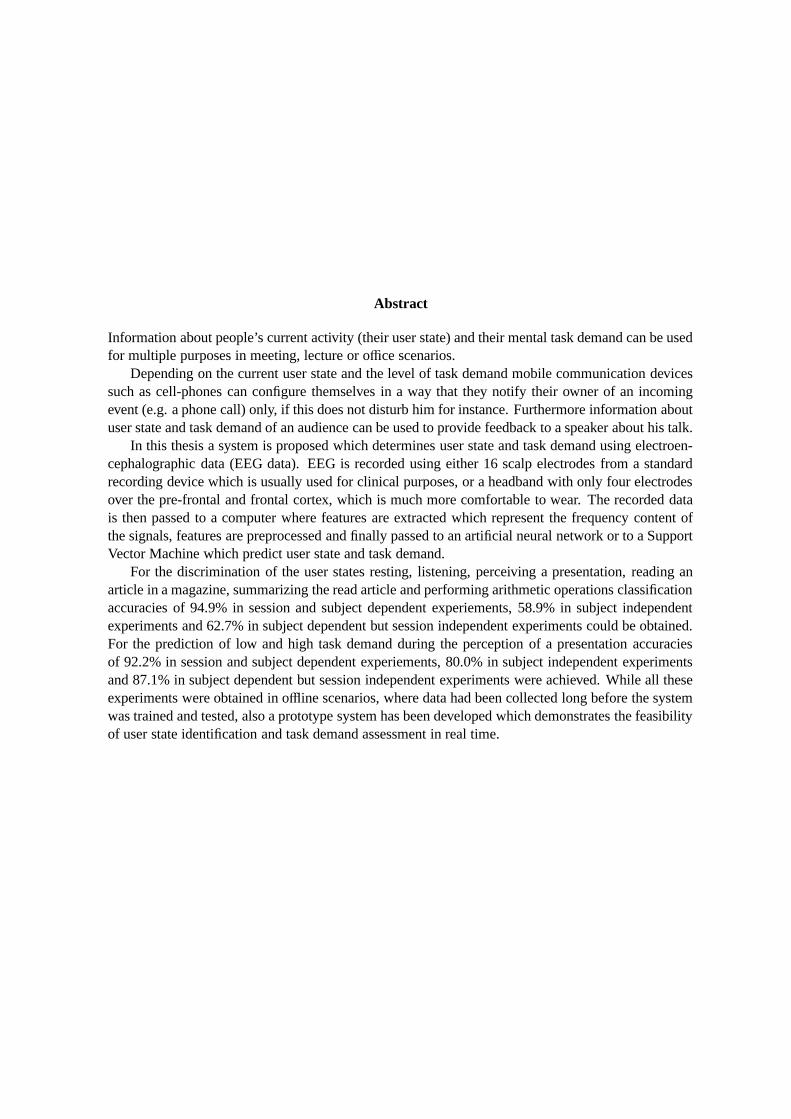
Abstract
Information about people’s current activity (their user state) and their mental task demand can be usedfor multiple purposes in meeting, lecture or office scenarios.
Depending on the current user state and the level of task demand mobile communication devicessuch as cell-phones can configure themselves in a way that they notify their owner of an incomingevent (e.g. a phone call) only, if this does not disturb him for instance. Furthermore information aboutuser state and task demand of an audience can be used to provide feedback to a speaker about his talk.
In this thesis a system is proposed which determines user state and task demand using electroen-cephalographic data (EEG data). EEG is recorded using either 16 scalp electrodes from a standardrecording device which is usually used for clinical purposes, or a headband with only four electrodesover the pre-frontal and frontal cortex, which is much more comfortable to wear. The recorded datais then passed to a computer where features are extracted which represent the frequency content ofthe signals, features are preprocessed and finally passed to an artificial neural network or to a SupportVector Machine which predict user state and task demand.
For the discrimination of the user states resting, listening, perceiving a presentation, reading anarticle in a magazine, summarizing the read article and performing arithmetic operations classificationaccuracies of 94.9% in session and subject dependent experiements, 58.9% in subject independentexperiments and 62.7% in subject dependent but session independent experiments could be obtained.For the prediction of low and high task demand during the perception of a presentation accuraciesof 92.2% in session and subject dependent experiements, 80.0% in subject independent experimentsand 87.1% in subject dependent but session independent experiments were achieved. While all theseexperiments were obtained in offline scenarios, where data had been collected long before the systemwas trained and tested, also a prototype system has been developed which demonstrates the feasibilityof user state identification and task demand assessment in real time.

Acknowledgments
At this place I would like to thank the many people who helped me to complete this thesis. First ofall, all the volunteers must be mentioned who allowed me to collect their EEG data, particularly thestudents from Carnegie Mellon University and the people from the second floor of the ”Insterburg” inKarlsruhe. Next I would like to thank Dana Burlan who helped me during the data collection and whosewed in the electrodes in the EEG-recording-headband with skillful hands.
Very special thanks go to my wife Laura who often assisted me during the data collections, whovolunteered for many data collections herself, who helped me to produce a demo video, who proof-read this manuscript and last but not least who was always there for me in times when I found itdifficult to carry on with this thesis.
Finally I would like to thank my supervisor Tanja Schultz for all the valuable discussions and thecomments to my work which significantly improved its quality.

Chapter 1
Introduction
In modern office or meeting environments people interact with each other in various ways: (mobile)electronic devices such as cell phones, PDAs and laptops are used to communicate via speech or textbut also face-to-face meetings take place frequently nowadays.
Information about user state, i.e. the current activity of an individual and mental task demand,i.e. the amount of mental resources required to execute the current activity, can provide importantinformation about the individuals needs and wishes concerning interaction. This information couldbe exploited for example by communication devices which select the kinds of notifications a userreceives appropriately according to the user’s current state and mental task demand level. On theother hand information about the predominant state and the task demand level of his audience canrepresent an interesting feedback for a speaker about a talk.
We refer to the current activity of an individual as user state in this work to emphasize that wesee a major purpose of gathering such activity information to improve the interfaces between com-munication devices and their users. To characterize the predominant activity of an audience during ameeting or a lecture, the term ”audience state” or ”participant state” would probably be more appro-priate. Note however that technically speaking a listener of a talk can also be seen as a ”user” whoobtains information from a ”device”, namely the speaker, via an ”interface”, which is the talk of thespeaker1 . Therefore and for reasons of clarity only the term user state is used in this work to character-ize an individual’s current activity. Note furthermore that the more general term task demand insteadof mental task demand is used in the following for simplicity, although we are exclusively concernedwith mental and not with physical task demand in this work.
1.1 Goal
The major goal of the research work described in this thesis is the development of a system whichautomatically identifies the user state and estimates the task demand level of an individual from hiselectrical brain activity, i.e. his electroencephalogram (EEG). In particular such a system shall beable to determine user state and task demand level in meeting, lecture or office scenarios such that theobtained information can be used to improve the interaction with and via electronic communicationdevices and face-to-face interaction between individuals. (Examples illustrating the relevance of user
1This point of view is even more justified when the human speaker is replaced by a computer system providing onelistener or an audience with information about a specific topic which is not a too unrealistic vision in times of modern dialogand information retrieval systems.

1.2 Motivation 3
state and task demand information for applications in the mentioned scenarios are given in the nextsection.)
Several subgoals emerge from this major goal:
• Robustness: Users must be allowed to talk and to move freely during EEG recording in anoffice or meeting environment which introduces usually large artifacts in the data. During clin-ical EEG recording data artifacts are reduced by requiring the patients not to talk and to remainimmobile in a fixed position during the whole recording which is clearly not acceptable for theapplications we are aiming at. Therefore the proposed system must be able to cope with allkinds of artifacts introduced in the data by moving and talking, i.e. it must be robust towardsthese artifacts.
• Acceptability: The sensors for EEG recording should disturb the user as little as possible andthe user must find his outer appearance still acceptable while wearing them. During clinicalEEG recording usually more than 20 scalp electrodes are placed all over the head. Prior to therecording intensive preparation of the patient is required to assure good data quality: electrodepositions must be determined exactly, the scalp is cleaned using alcohol and conductive paste inthe patients hair is required to establish a good conductivity between skin and electrode. The useof electrodes at positions all over the head and intensive user preparation is clearly not possiblefor the scenarios we are considering here. Ideally very few electrodes should be used which theuser can attach quickly himself. Furthermore conductive paste must not get into contact withthe user’s hair.
• Real time behavior: It must be possible to determine user state and task demand informationin real time, to allow for immediate reactions when these parameters change.
• Realistic scenarios: The user states to be considered here must be typical for real world meet-ing, lecture or office scenarios. Typical states are reading, typing, listening to a talk, perceivingan audio-visual presentation, talking or resting for example. Also task demand variations mustbe measured during realistic activities such as listening to a talk. As a mid-term goal the devel-oped system shall be used and evaluated in real meetings, lectures or office work places.
Note that the research work described in this thesis is just a first attempt towards user state identi-fication and task demand estimation in meeting or office scenarios. Therefore the aspects enumeratedabove are realized only to a certain extend in the proposed system (see also chapter 7). Results arepromising however and we are confident that some further research and development will allow tofulfill the afore mentioned goals even better.
1.2 Motivation
The most important motivation for the development of a system which determines user state andtask demand is to allow for more intelligent interaction between individuals and their communicationdevices and to make communication between individuals more effective. Concrete examples whichillustrate how the obtained information can be used for these purposes are presented in the following.
1.2.1 Human-Machine Interaction
Modern communication devices can be configured in various ways. In particular, different kinds ofnotifications (e.g. audio, visual or tactile notifications) can be chosen to announce different events
1.2 Motivation 4
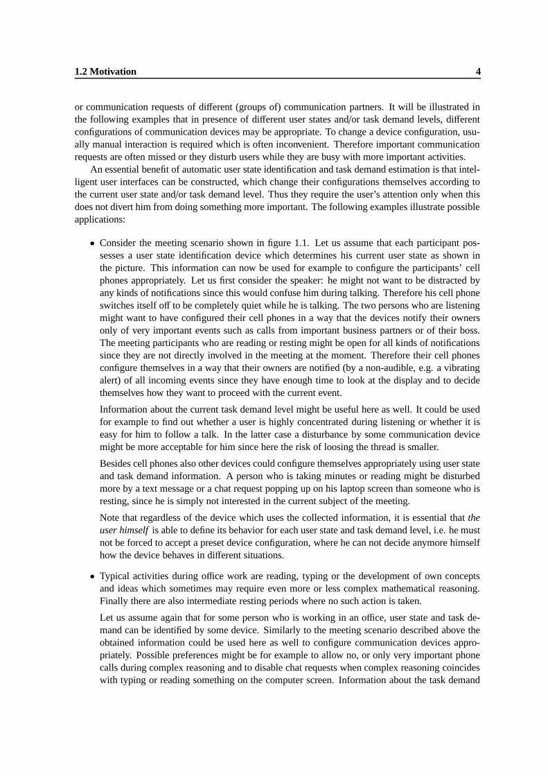
or communication requests of different (groups of) communication partners. It will be illustrated inthe following examples that in presence of different user states and/or task demand levels, differentconfigurations of communication devices may be appropriate. To change a device configuration, usu-ally manual interaction is required which is often inconvenient. Therefore important communicationrequests are often missed or they disturb users while they are busy with more important activities.
An essential benefit of automatic user state identification and task demand estimation is that intel-ligent user interfaces can be constructed, which change their configurations themselves according tothe current user state and/or task demand level. Thus they require the user’s attention only when thisdoes not divert him from doing something more important. The following examples illustrate possibleapplications:
• Consider the meeting scenario shown in figure 1.1. Let us assume that each participant pos-sesses a user state identification device which determines his current user state as shown inthe picture. This information can now be used for example to configure the participants’ cellphones appropriately. Let us first consider the speaker: he might not want to be distracted byany kinds of notifications since this would confuse him during talking. Therefore his cell phoneswitches itself off to be completely quiet while he is talking. The two persons who are listeningmight want to have configured their cell phones in a way that the devices notify their ownersonly of very important events such as calls from important business partners or of their boss.The meeting participants who are reading or resting might be open for all kinds of notificationssince they are not directly involved in the meeting at the moment. Therefore their cell phonesconfigure themselves in a way that their owners are notified (by a non-audible, e.g. a vibratingalert) of all incoming events since they have enough time to look at the display and to decidethemselves how they want to proceed with the current event.
Information about the current task demand level might be useful here as well. It could be usedfor example to find out whether a user is highly concentrated during listening or whether it iseasy for him to follow a talk. In the latter case a disturbance by some communication devicemight be more acceptable for him since here the risk of loosing the thread is smaller.
Besides cell phones also other devices could configure themselves appropriately using user stateand task demand information. A person who is taking minutes or reading might be disturbedmore by a text message or a chat request popping up on his laptop screen than someone who isresting, since he is simply not interested in the current subject of the meeting.
Note that regardless of the device which uses the collected information, it is essential that theuser himself is able to define its behavior for each user state and task demand level, i.e. he mustnot be forced to accept a preset device configuration, where he can not decide anymore himselfhow the device behaves in different situations.
• Typical activities during office work are reading, typing or the development of own conceptsand ideas which sometimes may require even more or less complex mathematical reasoning.Finally there are also intermediate resting periods where no such action is taken.
Let us assume again that for some person who is working in an office, user state and task de-mand can be identified by some device. Similarly to the meeting scenario described above theobtained information could be used here as well to configure communication devices appro-priately. Possible preferences might be for example to allow no, or only very important phonecalls during complex reasoning and to disable chat requests when complex reasoning coincideswith typing or reading something on the computer screen. Information about the task demand

1.2 Motivation 5
Figure 1.1: A typical meeting. Picture taken from [Student Government, University of Maine, 2005]
level might help here to make more fine grained decisions: communication requests might beless disturbing while reading an article which is easy to understand in contrast to another articlewith a more difficult contents for example. Also during routine tasks (e.g. reading or writinge-mails) some people might want to constrain the potential communication requests they arewilling to receive since they want to get their work done quickly. On the other hand they wouldlike to be notified of all kinds of communication requests (also of those which have previouslybeen rejected) when they are idle, such as during resting periods. Consequently it might bedesirable in an office environment to have intelligent devices.
1.2.2 Enhance Face-to-Face Communication
User state and task demand can provide important feedback about how perceived in a face-to-facecommunication. This is illustrated in the following two examples.
• During a meeting or a lecture it is usually very difficult for the speaker to tell whether his talkis too easy or too difficult for his audience or whether he is talking about a subject of commoninterest or not. Information about the predominant user state of his audience and its average taskdemand could help the speaker to find out how his talk is perceived. Low task demand couldbe seen as a hint to proceed faster while high task demand (or even overload) might indicate onthe other hand that the current topic must be explained more clearly. This could be particularhelpful in a lecturing or teaching scenario.
User state information could be used here to find out whether the audience is interested at all inthe current topic. This might not be the case if the predominant user state is something else thanlistening. Furthermore, user state information is important to retrieve out the precise reasons forhigh task demand: While a user’s task demand is constantly high, he can either listen attentivelyto the presentation and watch the slides (user state ”audiovisual perception”) or that he can reada paper which requires a lot of mental effort.
• Another interesting application in this context is to improve an information retrieval and dialogsystem which provides multi modal information about a selected topic to a user. If the systemdetects high task demand or even overload it might use this as an indicator that the user can’t

1.2 Motivation 6
keep up anymore with the current presentation and thus it could come up with other explana-tions. Note that also explicit interaction between listener and system is possible and perhapseven desirable in such situations. However the information how familiar the user is with differ-ent aspects of a certain topic, which can be perhaps inferred from the course of his task demand,might help to select the most appropriate explanations.
• Now let us consider two people who cannot communicate in a common language and thereforeuse a speech translation device to talk to each other. In this case, it is usually difficult to tellwhether the translation of what was just said is correct, i.e. if the dialog partner understoodthe meaning of the utterance as it was originally intended in the source language. If now theconfusion of the dialog partner could be measured when he hears the translated utterance, thisinformation could be used as an indicator for the translation quality. Note that the parameterstask demand and user state are not used here explicitly, however it might be a plausible hypoth-esis that the degree of confusion is correlated with the degree of task demand, since a confuseduser will mobilize more mental resources to determine the meaning of an utterance he could notunderstand at once.
This hypothesis is supported by findings from [Applied Anthropology Institute, 2001] and [De-fayolle et al., 1971] who report that mental confusion is often associated with the state of ”ex-treme alertness” which can be identified by distinct patterns in the EEG. (For the relation be-tween alertness and task demand please refer to section 2.3.2.) In these studies a very high de-gree of confusion, leading often to disorganized behavior, has been considered however. There-fore it remains to be investigated whether EEG correlates of confusion can also be detected inthe above described scenario.
1.2.3 Measure Usability
Probably task demand information can be used as well for the evaluation of the usability of interfaces.Using the underlying hypothesis that an electronic device (e.g. a cell phone, a PDA, a radio, an aircondition or a navigation system in a car) which is difficult to operate requires higher mental resourcesduring operation, task demand could be used directly as an indicator for usability. Thus EEG basedtask demand estimation could be used as a tool in ergonomics.
Although a few years ago it has been proposed to use EEG for usability assessment [Beer et al.,2003], to our current knowledge no research has been conducted yet which provides evidence for oragainst the above hypothesis. Only the relations between EEG and attitude, satisfaction or acceptancein the domain of user interface design have been investigated [Nielsen, 1993].
Note that for many aforementioned applications EEG data is certainly not the only source of infor-mation. Other physiological parameters such as the electrocardiogram (the ECG, i.e. the electricalheart activity) or the electromyogram (the EMG, i.e. the electrical muscular activity), methods likeeye tracking or head tracking and other techniques from computer vision or speech and language pro-cessing can certainly provide useful information for these applications as well. Physiological data andparticularly EEG data seem however to be complementary in many aspects to these other modalitieswhich makes their investigation particularly interesting here. A fusion of different modalities shouldbe an important goal towards the development of intelligent user interfaces and tools which enhancecommunication between individuals.

1.3 Ethical Considerations 7
1.3 Ethical Considerations
When user state or mental task demand are determined from individuals in every day situations, verypersonal and sensitive data is collected. Thus it is important to handle this data very carefully since itmight easily be used to offend peoples privacy. The performance of employees or their actions couldbe easily tracked using the recorded data. User state information might be used for example to find outhow much time people spend on other than work tasks during their office hours; information aboutmental task demand during the execution of a specific task could indicate how well an applicant issuited for a certain position.
The research work reported in this thesis has clearly not been done to encourage the developmentof applications aiming at these or similar purposes.
Rather then to control the user, the collected information should be used to give the user bettercontrol over his environment. As mentioned above, one reason to determine user state and task de-mand is to enhance the user’s ability to interact with electronic devices and to enable these devicesto behave according to the users wishes without requiring explicit input. However this can only begranted if the user has complete control over the collected information and over the devices using it.That means in particular that the user must be able to choose desired device configurations for a givenuser state and/or task demand level himself and he must not be forced to accept any preset configura-tion. The latter might for example lead to a situation where in order to increase the productivity of anemployee, phone calls, text messages etc. from his family or friends are blocked while he is not in theuser state of resting. This would take him away from controlling the use of the collected data whichis clearly not desirable.
In this context it is also important to point out the difference between this work and the DARPAAugmented Cognition (AugCog) program where important goals are the identification of cognitivestates and the assessment of mental task demand [Schmorrow and Kruse, 2002]. In the AugCogprogram the information about cognitive states shall be used to increase operator performance bypresenting him information appropriately according to his current state and thus to avoid cognitiveoverload. That implies that the operator has to allow the recording of his cognitive state continuouslyin order to be able to fulfill the task assigned to him. He has no choice how data is presented tohim, i.e. which view of the real data he can see. This might arouse the feeling of the operator thathe is degraded to a kind of ”computer” himself which has to fulfill a certain task without having thecontrol over the whole situation. While this may be appropriate for some military applications, it isnot acceptable for an individual in a office or meeting environment. Here everyone must be able tocontrol himself how and when which kind of information is presented to him, i.e. he must be able toconfigure the devices around him himself as mentioned above. Additionally it is important that usersshould wear EEG devices only voluntarily and they should always be able to switch them off.
Furthermore the user must know exactly what happens with the collected data and it must be hisown decision whether he wants to share the data with others, e.g. with a speaker to give him feedbackabout his talk, or not. In the meeting or lecture scenario described above, it is important that forprivacy reasons the speaker can only see the predominant user state and the average task demand ofhis audience but that the data of particular individuals remains hidden to him. Otherwise such datamight be used for example to find out which students do not listen to a lecture or which employees donot pay attention during a presentation of their boss.
Finally EEG devices for user state and task demand recordings should be preferably personaldevices used only by their owner, since this allows him to record information about his mental stateand his task demand whenever he wants and use it for the purpose he wants to use it. Also for hygienicreasons users may not want to wear an EEG device which has been previously used by someone else

1.4 Contributions 8
(unless it has been cleaned thoroughly which is time consuming).
1.4 Contributions
In this research work several state-of-the-art techniques from the domains of machine learning andsignal processing are applied to the problems of user state identification and task demand estimationfrom EEG data. The selection of appropriate methods, their combination, their adaptation to the spe-cific requirements of EEG data and finally the careful evaluation and discussion of their performancerepresent important scientific contributions of this research.
As already mentioned, the research work presented here is to be seen as a first attempt to constructa system for user state identification and task demand estimation using EEG data in every day meeting,lecture or office scenarios. To date, no publications could be found concerning the application ofEEG data in these scenarios. Particularly the attempt to reach the goals formulated in section 1.1distinguishes this work from other research which is concerned with computational processing ofEEG data.
Also two more practical contributions shall be pointed out here which address the goals formulatedin section 1.1:
• To illustrate the feasibility recording devices which are more comfortable to wear than standardclinical equipment, a headband with four build-in electrodes has been developed (see figure5.2). This can be seen as a first step towards recording devices which are more acceptable towear in every day situations.
• Furthermore a prototype system has constructed which demonstrates that the identification ofrealistic user states is possible in real time and in a scenario which has little in common with thewell defined laboratory conditions during clinical EEG recording (see section 6.1.10). Note thatthe same user states and the same recording conditions were also used for the data collectionconducted in this work (see chapter 5).
1.5 Overview
Figure 1.2 gives an overview of the developed system and illustrates the tasks to be accomplished toderive a hypothesis for the current user state and task demand level from the raw EEG data. For eachof the task one or more possible methods are investigated.
As a first step, artifacts introduced in the raw EEG data (50Hz or 60Hz AC noise, muscular ac-tivity, eye movements etc.) must be eliminated. We concentrate here on eye activity related artifactsand attempt to use independent component analysis (ICA) for their detection and removal. From theartifact free data feature vectors are extracted representing the frequency content of the data using ashort time Fourier transform (STFT). Then averaging over a history of k feature vectors is performedand features are normalized to reduce natural fluctuations and unwanted variability in the data. Sincethe feature space has a very high dimension, the benefit of feature reduction methods is investigated.Finally artificial neural networks (ANNs) and support vector machines (SVMs) are used as classifi-cation techniques for user state identification. These classification techniques are also applicable forthe estimation of different task demand levels. However since task demand is an ordinally scaledparameter, also variants of ANNs and SVMs for regression estimation and a simple linear model(OLS-Regression) are applied for this purpose.
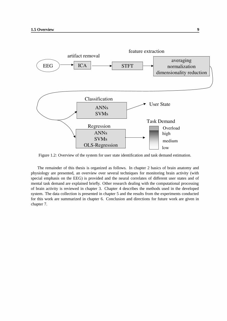
1.5 Overview 9
Figure 1.2: Overview of the system for user state identification and task demand estimation.
The remainder of this thesis is organized as follows. In chapter 2 basics of brain anatomy andphysiology are presented, an overview over several techniques for monitoring brain activity (withspecial emphasis on the EEG) is provided and the neural correlates of different user states and ofmental task demand are explained briefly. Other research dealing with the computational processingof brain activity is reviewed in chapter 3. Chapter 4 describes the methods used in the developedsystem. The data collection is presented in chapter 5 and the results from the experiments conductedfor this work are summarized in chapter 6. Conclusion and directions for future work are given inchapter 7.

Chapter 2
Bio-Medical Background
Our ability to observe the activity of the living brain is very limited. Current techniques for monitor-ing brain activity can only provide information about an extremely small fraction of those processeswhich are responsible for our actions, our thinking and also our consciousness. To give the reader animpression of the huge complexity of the brain, section 2.1 reviews briefly basics of brain anatomyand physiology. A special emphasis is put on those processes causing the EEG. In section 2.3 neuralcorrelates and in particular EEG correlates of different mental states and of varying task demand lev-els are explained which represent the bio-medical foundation for the research presented here. Finallysome none-invasive techniques for monitoring brain activity are introduced in section 2.2 and it willbecome clear that due to limitations in spatial or temporal resolution of these techniques, to date onlyvery incomplete information about ongoing processes in the brain can be visualized.
2.1 Anatomy and Physiology of the Brain
The human’s central nervous system consists of the spinal cord and the brain. One of its tasks is toprocess and to integrate incoming sensory stimuli which are received via peripheral nerves (afferences)and to give impulses back to actuators, e.g. to muscles or glands (efferences) which cause automaticor voluntary action. Furthermore the central nervous system, particularly the brain, is responsiblefor higher integrative abilities such as thinking, learning, production and understanding of speech,memory, emotion etc. Finally vegetative functions such as respiration and the cardio-vascular systemare controlled by the central nervous system.
2.1.1 Brain Anatomy
Anatomically five basic parts of the brain can be distinguished [Faller, 1995] as shown in figure 2.1:
Cerebrum: The cerebrum which is located directly under the skull surface is the largest part ofthe brain. Its main functions are the initiation of complex movement, speech and languageunderstanding and production, memory and reasoning. Brain monitoring techniques whichmake use of sensors placed on the scalp mainly record activity from the outermost part of thecerebrum, the cortex. More inside the cerebrum the basal ganglions can be found which consistof a number of nuclei controlling the extend and the direction of slow movements. Also thethalamus is located here which directs sensory information to appropriate parts of the cortex. Amore detailed explanation of the cortex anatomy is given below, since this becomes particularlyimportant in later sections of this work.

2.1 Anatomy and Physiology of the Brain 11
Figure 2.1: Different anatomical parts of the human brain, with modifications from [Scientific Learn-ing Cooperation, 1999]
Diencephalon: One important function of the diencephalon is the forwarding of sensory informationto other brain areas. Besides that, it contains the hypothalamus which controls the body tem-perature, the water balance and the ingestion to assure the state of homeostasis for the body, i.e.”good working conditions” for all body cells.
Cerebellum: The coordination of all kinds of movements is done in the cerebellum. Therefore itcooperates closely with structures from the cerebrum (e.g. the basal ganglions). Cerebellumand cerebrum are connected via the Pons.
Mesencephalon: The largest part of the reticular system (the formatio reticularis) is located here. Itcontrols vigilance and the sleep-wake rhythm.
Medulla oblongata: The medulla oblongata connects the brain with the spinal cord. Respiration andthe cardiovascular system are controlled by that part of the central nervous system. Furthermorea huge number of peripheral nerves pass through the medulla oblongata.
Compared to the brains of other mammals, the human brain has the largest and best developedcortex. Neural processes related to abilities like complex reasoning, speech and language etc. whichdistinguish humans from other mammals take place in that part of the brain.
The cortex consists of two hemispheres which are connected via a beam called corpus callosum(see figure 2.1). Each hemisphere is dominant for particular abilities. For right handed persons theright hemisphere is activated more during the recognition of geometric patterns, spatial orientation,the use non verbal memory and the recognition of non-verbal noises while more activity in the lefthemisphere can be observed during the recognition of letters and words, the use verbal memory andauditory perception of words and language. Note however that this hemispheric asymmetry is usuallynot very pronounced and in cases of injuries one hemisphere is often able to fulfill tasks for which theother one was previously dominant [Schmidt and Thews, 1997].
2.1 Anatomy and Physiology of the Brain 12
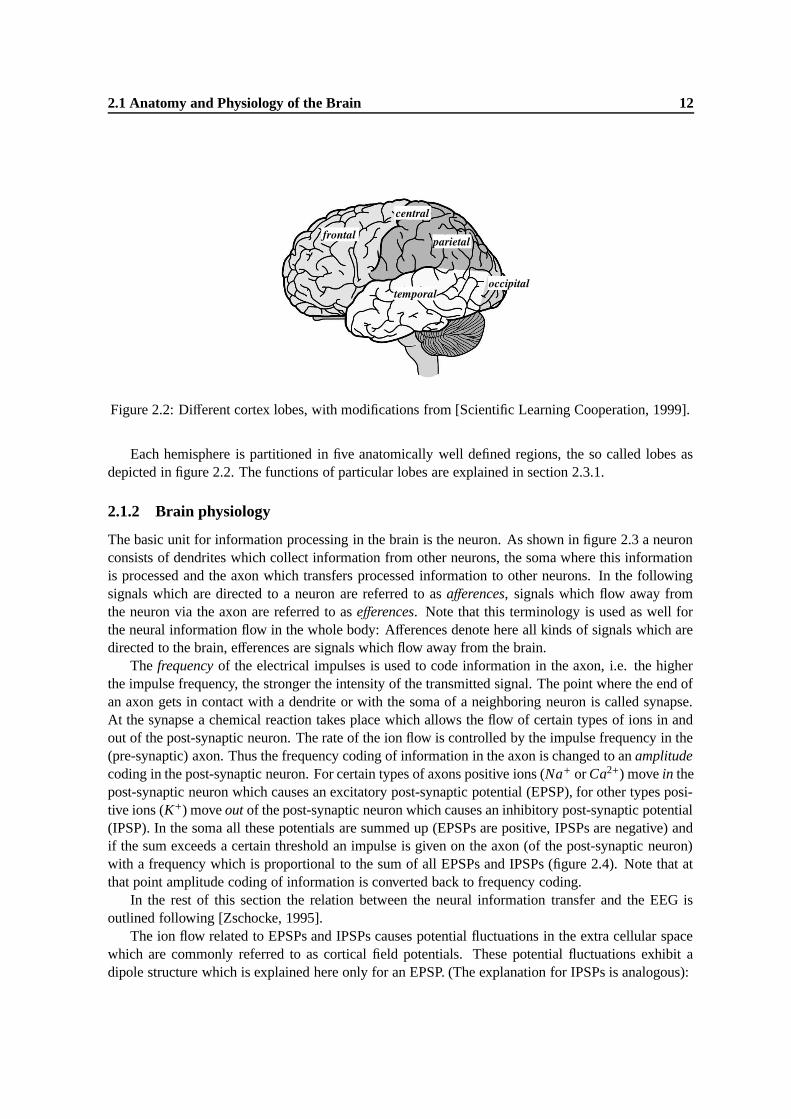
Figure 2.2: Different cortex lobes, with modifications from [Scientific Learning Cooperation, 1999].
Each hemisphere is partitioned in five anatomically well defined regions, the so called lobes asdepicted in figure 2.2. The functions of particular lobes are explained in section 2.3.1.
2.1.2 Brain physiology
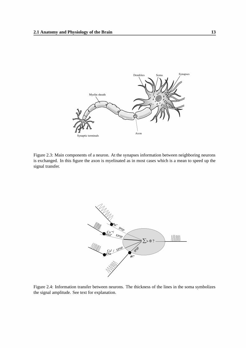
The basic unit for information processing in the brain is the neuron. As shown in figure 2.3 a neuronconsists of dendrites which collect information from other neurons, the soma where this informationis processed and the axon which transfers processed information to other neurons. In the followingsignals which are directed to a neuron are referred to as afferences, signals which flow away fromthe neuron via the axon are referred to as efferences. Note that this terminology is used as well forthe neural information flow in the whole body: Afferences denote here all kinds of signals which aredirected to the brain, efferences are signals which flow away from the brain.
The frequency of the electrical impulses is used to code information in the axon, i.e. the higherthe impulse frequency, the stronger the intensity of the transmitted signal. The point where the end ofan axon gets in contact with a dendrite or with the soma of a neighboring neuron is called synapse.At the synapse a chemical reaction takes place which allows the flow of certain types of ions in andout of the post-synaptic neuron. The rate of the ion flow is controlled by the impulse frequency in the(pre-synaptic) axon. Thus the frequency coding of information in the axon is changed to an amplitudecoding in the post-synaptic neuron. For certain types of axons positive ions (Na+ or Ca2+) move in thepost-synaptic neuron which causes an excitatory post-synaptic potential (EPSP), for other types posi-tive ions (K+) move out of the post-synaptic neuron which causes an inhibitory post-synaptic potential(IPSP). In the soma all these potentials are summed up (EPSPs are positive, IPSPs are negative) andif the sum exceeds a certain threshold an impulse is given on the axon (of the post-synaptic neuron)with a frequency which is proportional to the sum of all EPSPs and IPSPs (figure 2.4). Note that atthat point amplitude coding of information is converted back to frequency coding.
In the rest of this section the relation between the neural information transfer and the EEG isoutlined following [Zschocke, 1995].
The ion flow related to EPSPs and IPSPs causes potential fluctuations in the extra cellular spacewhich are commonly referred to as cortical field potentials. These potential fluctuations exhibit adipole structure which is explained here only for an EPSP. (The explanation for IPSPs is analogous):
2.1 Anatomy and Physiology of the Brain 13
Figure 2.3: Main components of a neuron. At the synapses information between neighboring neuronsis exchanged. In this figure the axon is myelinated as in most cases which is a mean to speed up thesignal transfer.
Figure 2.4: Information transfer between neurons. The thickness of the lines in the soma symbolizesthe signal amplitude. See text for explanation.
2.1 Anatomy and Physiology of the Brain 14
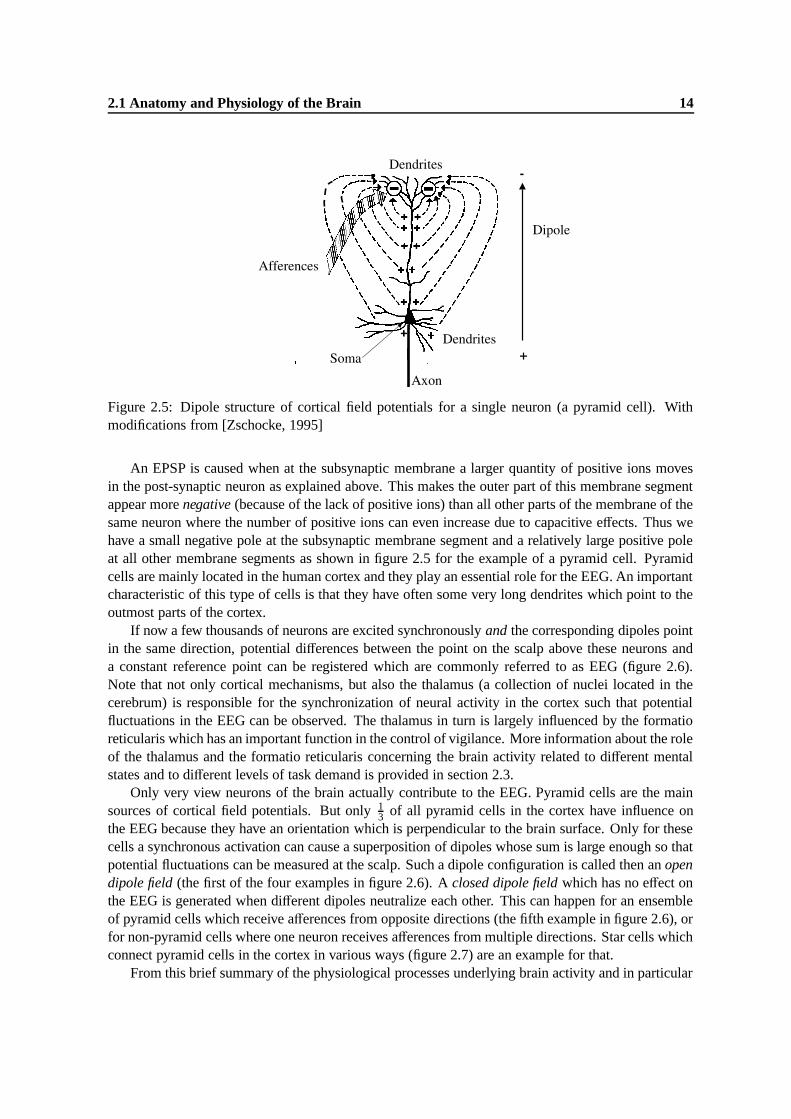
Figure 2.5: Dipole structure of cortical field potentials for a single neuron (a pyramid cell). Withmodifications from [Zschocke, 1995]
An EPSP is caused when at the subsynaptic membrane a larger quantity of positive ions movesin the post-synaptic neuron as explained above. This makes the outer part of this membrane segmentappear more negative (because of the lack of positive ions) than all other parts of the membrane of thesame neuron where the number of positive ions can even increase due to capacitive effects. Thus wehave a small negative pole at the subsynaptic membrane segment and a relatively large positive poleat all other membrane segments as shown in figure 2.5 for the example of a pyramid cell. Pyramidcells are mainly located in the human cortex and they play an essential role for the EEG. An importantcharacteristic of this type of cells is that they have often some very long dendrites which point to theoutmost parts of the cortex.
If now a few thousands of neurons are excited synchronously and the corresponding dipoles pointin the same direction, potential differences between the point on the scalp above these neurons anda constant reference point can be registered which are commonly referred to as EEG (figure 2.6).Note that not only cortical mechanisms, but also the thalamus (a collection of nuclei located in thecerebrum) is responsible for the synchronization of neural activity in the cortex such that potentialfluctuations in the EEG can be observed. The thalamus in turn is largely influenced by the formatioreticularis which has an important function in the control of vigilance. More information about the roleof the thalamus and the formatio reticularis concerning the brain activity related to different mentalstates and to different levels of task demand is provided in section 2.3.
Only very view neurons of the brain actually contribute to the EEG. Pyramid cells are the mainsources of cortical field potentials. But only 1
3 of all pyramid cells in the cortex have influence onthe EEG because they have an orientation which is perpendicular to the brain surface. Only for thesecells a synchronous activation can cause a superposition of dipoles whose sum is large enough so thatpotential fluctuations can be measured at the scalp. Such a dipole configuration is called then an opendipole field (the first of the four examples in figure 2.6). A closed dipole field which has no effect onthe EEG is generated when different dipoles neutralize each other. This can happen for an ensembleof pyramid cells which receive afferences from opposite directions (the fifth example in figure 2.6), orfor non-pyramid cells where one neuron receives afferences from multiple directions. Star cells whichconnect pyramid cells in the cortex in various ways (figure 2.7) are an example for that.
From this brief summary of the physiological processes underlying brain activity and in particular
2.2 Monitoring Brain Activity 15
Figure 2.6: Synchronized neuron activity causing potential differences which can be measured at thescalp. The dipoles are depicted by the arrows. Note that by convention positive potential differencescorrespond to amplitudes with downward orientation and negative potential differences to amplitudeswith upward orientation.
Figure 2.7: A closed dipole field generated by a star cell. Aff.: Afferences causing a negative pole atthe outer end of the dendrites.
of those processes generating the EEG, we conclude that most brain activity remains hidden to thismonitoring technique. Therefore EEG signals are certainly not suitable to make fine grained infer-ences about neural processes in the brain. In section 2.3 it will be explained however, that neverthelessa lot of information about mental states and mental task demand can be extracted from the potentialdifferences which are measured using scalp electrodes.
2.2 Monitoring Brain Activity
After in the previous section the mechanisms related to brain activity have been explained, severaltechniques for monitoring this activity shall be reviewed in this section. The following monitoringtechniques are commonly applied in the medical domain:

2.2 Monitoring Brain Activity 16
• Electroencephalography (EEG)
• Magnetoencephalogtaphy (MEG)
• Functional Magnetic Resonance Imaging (fMRI)
• Functional Near-Infrared Spectroscopy (fNIRS)
• Single Photon Emission Tomography (SPECT)
• Proton Emission Tomography (PET)
They can be classified using several characteristics:
• Intrusiveness
• Spatial resolution
• Temporal resolution
• Physiological parameter which is monitored
• Resources required for operation of the monitoring device
• Applicability as portable device
In this section the key ideas of the different monitoring techniques are explained and comparedaccording to the characteristics enumerated above. Since the experimental part of this work is focusedon EEG, this technique is reviewed in greater detail, following mainly [Zschocke, 1995] and [Bolzand Urbaszek, 2002] if no other reference is mentioned explicitly. A good description of all othermonitoring techniques can be found in [Dossel, 2000], except functional near infrared spectroscopywhich is described for example in [Izzetoglu et al., 2004].
2.2.1 The Electroencephalogram (EEG)
The EEG which can be recorded at the scalp has amplitudes between 0µV and 80µV and a frequencyrange between 0Hz and 80Hz [Schmidt and Thews, 1997]. For several reasons the potential differ-ences which can be measured between two points of the scalp are very different from those whichcould be measured when electrodes were implanted directly in the brain, i.e. when the activity of thepotential generators could be measured directly:
1. A superposition of potentials generated in different areas of the cortex is measured using scalpelectrodes since brain tissue and the liquor are conductive (volume conduction, figure 2.8).
2. The amplitude of the originally generated potential differences is attenuated because of theresistive properties of the tissue between the potential generators and the electrode (e.g. liquor,skin, bone of the skull).
3. Capacities caused by cell membranes and other inhomogeneities (e.g. liquor-skull, skull-skin)between potential generators and electrodes influence the amplitude of the EEG signals as afunction of their frequency as sketched in figure 2.10.
A diagram of the resistive and capacitive elements between potential generators and electrodes isdepicted in figure 2.9.
2.2 Monitoring Brain Activity 17
Figure 2.8: Volume conduction in the brain. Bold lines indicate a stronger impact on the measuredsignal, since the distance from the corresponding potential generator to the scalp electrode and thusthe total resistance is smaller.
Figure 2.9: Resistive and capacitive elements between potential generators and scalp electrodes ac-cording to [Dossel, 2000] and [Bolz and Urbaszek, 2002]. For simplicity only one tissue cell isshown. Re: resistance of the extra-cellular space (the liquor), Ri: resistance of the intra-cellular space,Rm: membrane resistance, Cm: membrane capacity, Rs: resistance of skin and skull, Cs: capacityrepresenting all inhomogeneities at the boundary of liquor, skin and skull.
2.2 Monitoring Brain Activity 18
Figure 2.10: Influence of capacities caused by inhomogeneities between potential generators andelectrodes on the EEG amplitude as a function of EEG frequency. Sketched using a few data pointsfrom [Meyer-Waarden, 1985]
2.2.1.1 Electrode Positions
The positions for EEG electrodes should be chosen in a way, that all cortex regions which mightexhibit interesting EEG patterns are covered. For most applications this is usually the whole cortex.An internationally accepted standard for electrode placements is the 10-20 system1introduced in 1957by the International EEG Federation [Jasper, 1958]. During all experiments conducted for this workelectrodes were placed according to the 10-20 system.
Three anatomical reference points must be determined before the 10-20 system electrode positionscan be found (figure 2.11):
Nasion: The onset of the nose on the skull, below the forehead.
Inion: The bony protuberance which marks the transition between skull and neck.
Pre-auricular reference point: Located before the cartilaginous protrusion of the acoustic meatus(the auditory canal).
Figure 2.12 shows the 19 electrode positions of the 10-20 system in their projection on the cortex.The name for a particular electrode position reflects the anatomical region of the cortex above whichit is located. Fp stands for frontopolar, F for frontal, T for temporal, C for central P for parietal, O
1The reason for the name ”10-20 system” is that electrodes are placed at distances of 10% or 20% of the length of severalconnections between some reference points as described below.

2.2 Monitoring Brain Activity 19
Figure 2.11: Anatomical reference points which represent the starting points for finding the electrodepositions defined by the 10-20 system (with modifications from [Zschocke, 1995]).
for occipital and A for auricular. G denotes the ground electrode. Even numbers denote the right partof the head, odd numbers the left part. The following procedure can be used to find the electrodepositions using the above defined anatomical references as starting points:
1. The connection NI from nasion to inion via the top of the head is measured. Beginning from thenasion, the point Fpz is placed after 10% of NI, the electrodes Fz, Cz, Pz and the point Oz areplaced each after proceeding 20% of NI from the previous position. (No electrodes are locatedat the points Fpz and Oz but they are used to find the positions of other electrodes.)
2. The electrodes A1 and A2 are placed at the left and right ear lobes. The connection PA fromone pre-auricular reference point to the other one via the electrode position Cz (which has beendetermined before) is measured. After 10% of PA above both reference points the electrodesT3 and T4 are placed. 20% of PA above T3 and T4 the electrodes C3 and C4 are placed.
3. The connection FO1 between the point Fpz and Oz is measured via the position T3. Starting atFpz the electrode Fp1 is placed after 10% of FO1, the electrodes F7, T5 and O1 are placed eachafter proceeding 20% of FO1 from the previous electrode. In an analogous way the connectionFO2 between Fpz and Oz via T4 is measured and the electodes Fp2, F8, T6 and O2 are placedaccordingly.
4. The electrode F3 is placed at half the distance between F7 and Fz, the electrode P3 is placed athalf distance between T5 and PZ. In the same fashion the electrodes F4 and P4 are placed onthe other side of the head.
When recording EEG with commonly available EEG-caps or other standard recording devices,the procedure for determining the electrode positions needs not to be repeated prior to each dataacquisition session. However the accuracy of electrode placements often suffers when flexible EEG-caps are used. Although usually different caps exist for different head circumferences, it can not beguaranteed that for each individual electrodes are placed exactly at the positions defined by the 10-20-system. Therefore in clinical EEG recordings the whole procedure as described above is usuallycarried out prior to each session which is extremely time consuming but which guarantees on the otherhand exact electrode positions. For EEG recording in the context of user state identification and taskdemand assessment, it is important that electrodes can be attached very quickly. For that reason eitherflexible EEG-caps or other recording devices which are more comfortable to wear and even easier toattach (see also section 5.1) are suitable for that purpose.

2.2 Monitoring Brain Activity 20
Figure 2.12: Electrode positions of the 10-20 system (with modifications from [Zschocke, 1995])
The 19 electrodes of the 10-20 system are sufficient for most clinical purposes. Due to improvedamplifier technology, for special applications much more electrodes (up to 128) can be used, whichare usually placed according to various non-standardized conventions in each EEG laboratory. Notethat also extensions of the 10-20 system with a couple of more electrodes exist which are accepted asquasi-standards.
2.2.1.2 Electrode Montage
The term ”electrode montage” refers to the various ways in which the signals from different elec-trodes can be combined before amplification [Niedermeyer and da Silva, 1987]. Two generally dif-ferent methods for connecting EEG electrodes to the amplifier can be distinguished: bipolar electrodemontage and common-reference electrode montage. In both cases the EEG is measured differentially,i.e. the difference between the potential of two electrodes (or between one electrode and the averagedpotential of a set of electrodes) is measured.
For a common-reference montage the EEG signals represent the difference of the potentials ofeach electrode and one or more reference points which all electrodes (or at least a subset of electrodes)have in common. There are generally two criteria for good reference points:
1. They should be far enough away from the cortex, so that no brain activity is captured with thereference electrode.
2. They should be at a position where artifacts introduced by other physiological processes arelow.
Therefore a reference at the hand or at the legs, which would be ideal to fulfill the first criterion,is not reasonable, since large artifacts originating from the ECG would contaminate the signal in thatcase.
When only one reference point is used for all electrodes or for each subset of electrodes (naturalreference), electrode A1 is often used as reference for the EEG electrodes over the left half of the

2.2 Monitoring Brain Activity 21
cortex and electrode A2 for those over the right half. Another common choice is to use electrodeCz as reference for all other electrodes. As sets of reference electrodes whose potential is averagedbefore calculating the potential difference between EEG electrode and references the electrodes A1and A2 or even all electrodes can be used (technical reference). Although the latter case has someadvantages since artifacts introduced by one electrode from the reference set have a lower impact,it has the disadvantage of a spatial low pass. The activity of each electrode is mapped with a smallamplitude to all other electrode channels because each electrode is part of the reference set.
The idea of bipolar electrode montages is that always the difference between neighboring elec-trodes is taken. This has the large disadvantage that not the ”real” EEG, i.e. an approximation of thedipole configuration below each electrode is measured but the difference between the dipole configu-rations below adjacent electrodes. In the medical domain bipolar recordings are interesting howeverto detect the specific location of particular processes: if one process takes place below two electrodes,there will be a zero signal for the recording of exactly these two electrodes. A special case of a bipolarelectrode montage is the laplacian montage. Here all neighbors of one electrode (up to 8 electrodes)are included in the set of references. This is advantageous for some special clinical applications.
Finally ground electrodes are required to reduce noise from the AC power lines which is presentin the whole body and thus also contaminates the measured signals. Intuitively speaking the groundelectrode gives the noise signal the possibility to flow out of the body against a comparatively smallresistance. Therefore the noise takes preferably the path via the ground electrode and not via otherelectrodes so that the measured signal is contaminated less. (It is also possible to give a signal onthe ground electrode which is inverse to the noise signal, so that both signals annihilate. This is anappropriate mean for even more effective noise reduction.) In the 10-20 system the position for theground electrode is close in front of the position Fz (see figure 2.12). However also other positionsfor ground electrodes are possible as long as they capture as little muscular activity as possible, sincethis would introduce artifacts in all electrode channels.
2.2.1.3 Electrodes
Electrodes are the most critical components which determine the EEG signal quality. It is their task tomediate between the ion based transport of electrical charge in the tissue and the electron based chargetransport in copper wires which lead to the amplifier. In the tissue an electrolyte is responsible for theconduction of electricity. This is typically NaCl which dissociates to Na+ and Cl− ions in a waterysolution. The electrode however gets only in contact with the skin which is relatively dry and usuallynot permeable for the electrolyte in the body. Therefore it is essential to use an additional electrolyte(in form of electrode paste) which permeates the skin and thus establishes a connection between bodyelectrolyte and the metal phase of the electrode. As a consequence the resistance and the capacity ofthe skin (Rs and Cs is figure 2.9) decrease by some orders of magnitude when using electrode paste.Only this makes EEG recording possible.
The interaction between metal phase and electrolyte phase mainly determines the properties ofan electrode. Due to different electro-chemical properties of both phases electrons tend to movepreferably from metal to the electrolyte or vice versa, until a certain potential difference between bothphases is reached. This potential difference is called electrode potential or equilibrium potential sincechemical and electrical potential differences between electrolyte and metal are in the equilibrium here.Because of the electrode potential polar water molecules (which are contained in the electrolyte) attachthemselves at the boundary between both phases so that a double layer (ions and water molecules) isformed, the Helmholtz double layer. This double layer is not easily permeable for electrons andtherefore it represents a capacity (figure 2.13). Nevertheless an excess of electrons at either side of the
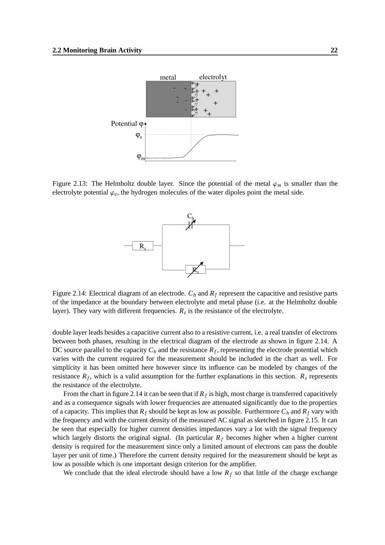
2.2 Monitoring Brain Activity 22
Figure 2.13: The Helmholtz double layer. Since the potential of the metal ϕm is smaller than theelectrolyte potential ϕe, the hydrogen molecules of the water dipoles point the metal side.
Figure 2.14: Electrical diagram of an electrode. Ch and R f represent the capacitive and resistive partsof the impedance at the boundary between electrolyte and metal phase (i.e. at the Helmholtz doublelayer). They vary with different frequencies. Rz is the resistance of the electrolyte.
double layer leads besides a capacitive current also to a resistive current, i.e. a real transfer of electronsbetween both phases, resulting in the electrical diagram of the electrode as shown in figure 2.14. ADC source parallel to the capacity Ch and the resistance R f , representing the electrode potential whichvaries with the current required for the measurement should be included in the chart as well. Forsimplicity it has been omitted here however since its influence can be modeled by changes of theresistance R f , which is a valid assumption for the further explanations in this section. Rz representsthe resistance of the electrolyte.
From the chart in figure 2.14 it can be seen that if R f is high, most charge is transferred capacitivelyand as a consequence signals with lower frequencies are attenuated significantly due to the propertiesof a capacity. This implies that R f should be kept as low as possible. Furthermore Ch and R f vary withthe frequency and with the current density of the measured AC signal as sketched in figure 2.15. It canbe seen that especially for higher current densities impedances vary a lot with the signal frequencywhich largely distorts the original signal. (In particular R f becomes higher when a higher currentdensity is required for the measurement since only a limited amount of electrons can pass the doublelayer per unit of time.) Therefore the current density required for the measurement should be kept aslow as possible which is one important design criterion for the amplifier.
We conclude that the ideal electrode should have a low R f so that little of the charge exchange
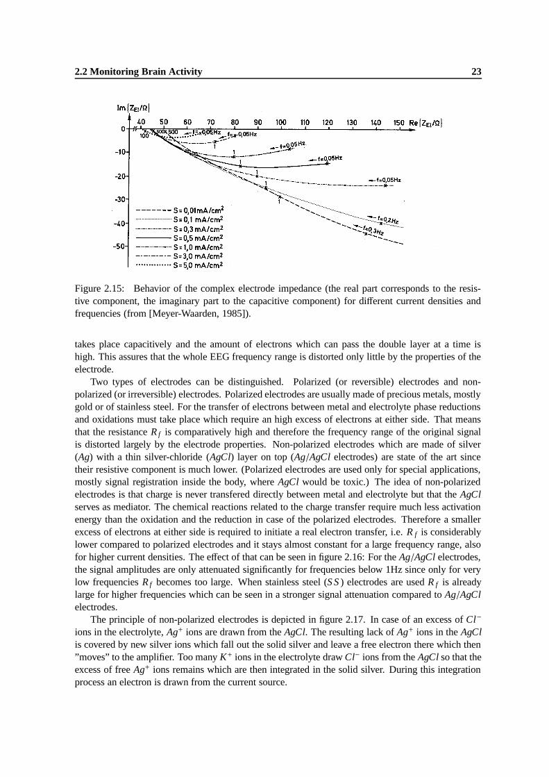
2.2 Monitoring Brain Activity 23
Figure 2.15: Behavior of the complex electrode impedance (the real part corresponds to the resis-tive component, the imaginary part to the capacitive component) for different current densities andfrequencies (from [Meyer-Waarden, 1985]).
takes place capacitively and the amount of electrons which can pass the double layer at a time ishigh. This assures that the whole EEG frequency range is distorted only little by the properties of theelectrode.
Two types of electrodes can be distinguished. Polarized (or reversible) electrodes and non-polarized (or irreversible) electrodes. Polarized electrodes are usually made of precious metals, mostlygold or of stainless steel. For the transfer of electrons between metal and electrolyte phase reductionsand oxidations must take place which require an high excess of electrons at either side. That meansthat the resistance R f is comparatively high and therefore the frequency range of the original signalis distorted largely by the electrode properties. Non-polarized electrodes which are made of silver(Ag) with a thin silver-chloride (AgCl) layer on top (Ag/AgCl electrodes) are state of the art sincetheir resistive component is much lower. (Polarized electrodes are used only for special applications,mostly signal registration inside the body, where AgCl would be toxic.) The idea of non-polarizedelectrodes is that charge is never transfered directly between metal and electrolyte but that the AgClserves as mediator. The chemical reactions related to the charge transfer require much less activationenergy than the oxidation and the reduction in case of the polarized electrodes. Therefore a smallerexcess of electrons at either side is required to initiate a real electron transfer, i.e. R f is considerablylower compared to polarized electrodes and it stays almost constant for a large frequency range, alsofor higher current densities. The effect of that can be seen in figure 2.16: For the Ag/AgCl electrodes,the signal amplitudes are only attenuated significantly for frequencies below 1Hz since only for verylow frequencies R f becomes too large. When stainless steel (S S ) electrodes are used R f is alreadylarge for higher frequencies which can be seen in a stronger signal attenuation compared to Ag/AgClelectrodes.
The principle of non-polarized electrodes is depicted in figure 2.17. In case of an excess of Cl−
ions in the electrolyte, Ag+ ions are drawn from the AgCl. The resulting lack of Ag+ ions in the AgClis covered by new silver ions which fall out the solid silver and leave a free electron there which then”moves” to the amplifier. Too many K+ ions in the electrolyte draw Cl− ions from the AgCl so that theexcess of free Ag+ ions remains which are then integrated in the solid silver. During this integrationprocess an electron is drawn from the current source.
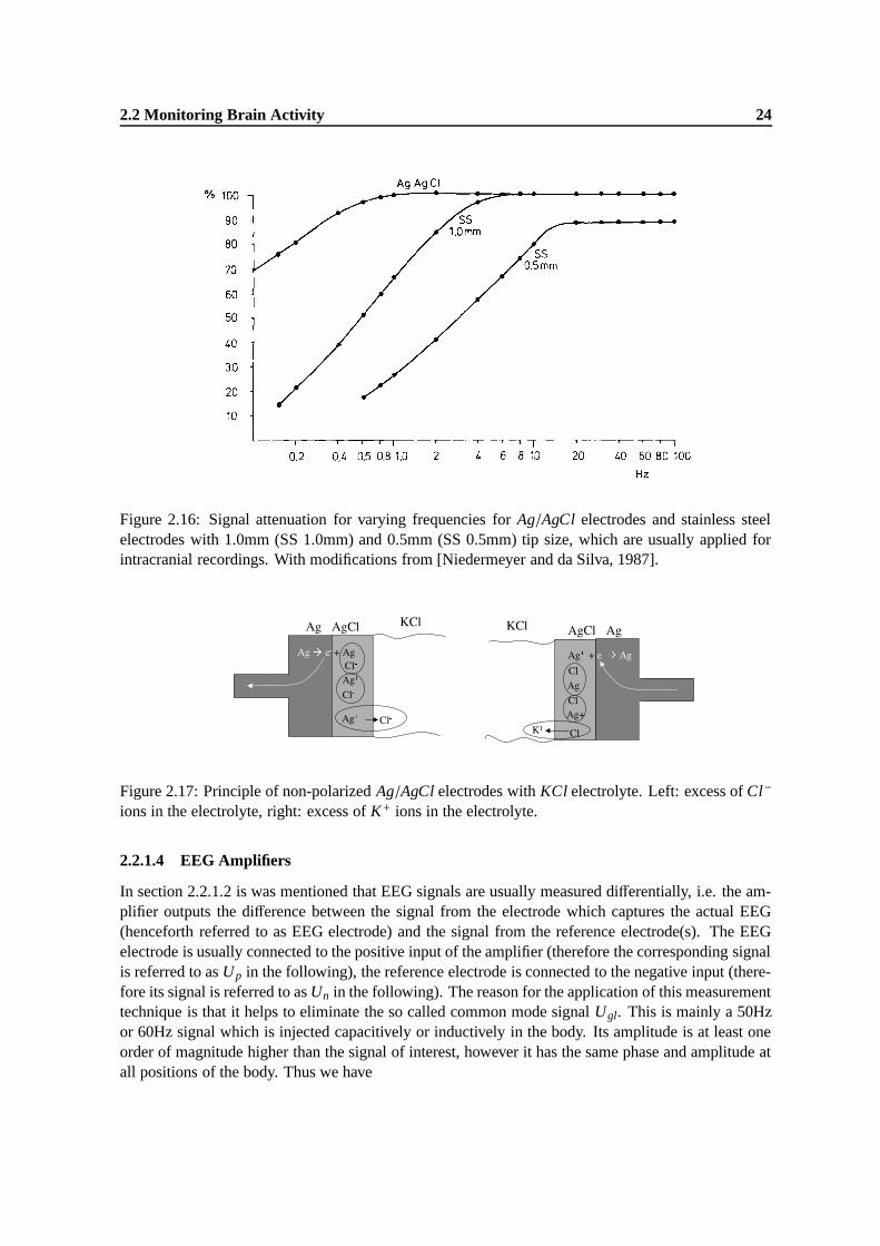
2.2 Monitoring Brain Activity 24
Figure 2.16: Signal attenuation for varying frequencies for Ag/AgCl electrodes and stainless steelelectrodes with 1.0mm (SS 1.0mm) and 0.5mm (SS 0.5mm) tip size, which are usually applied forintracranial recordings. With modifications from [Niedermeyer and da Silva, 1987].
Figure 2.17: Principle of non-polarized Ag/AgCl electrodes with KCl electrolyte. Left: excess of Cl−
ions in the electrolyte, right: excess of K+ ions in the electrolyte.
2.2.1.4 EEG Amplifiers
In section 2.2.1.2 is was mentioned that EEG signals are usually measured differentially, i.e. the am-plifier outputs the difference between the signal from the electrode which captures the actual EEG(henceforth referred to as EEG electrode) and the signal from the reference electrode(s). The EEGelectrode is usually connected to the positive input of the amplifier (therefore the corresponding signalis referred to as Up in the following), the reference electrode is connected to the negative input (there-fore its signal is referred to as Un in the following). The reason for the application of this measurementtechnique is that it helps to eliminate the so called common mode signal Ugl. This is mainly a 50Hzor 60Hz signal which is injected capacitively or inductively in the body. Its amplitude is at least oneorder of magnitude higher than the signal of interest, however it has the same phase and amplitude atall positions of the body. Thus we have

2.2 Monitoring Brain Activity 25
Figure 2.18: Principal of differential EEG measurement. See text for the explanation.
Up = UEEG + Ugl and Un = URe f + Ugl
where UEEG is the signal from the EEG electrode without the common mode noise and URe f thesignal from the reference electrode without the common mode noise. Using differential measurementsthe output signal Ua ideally does not contain the common mode noise Ugl anymore (figure 2.18).When it can be assumed furthermore that the signal URe f is mostly constant (URe f = C), the outputof the amplifier Ua differs only by an offset from the potential fluctuations at the electrode of interest.
Due to tolerances during the manufacturing of the electronic components of the amplifier thecommon mode signal is never rejected completely. Therefore Ua usually evaluates to
Ua = α1Up − α2Un (2.1)
= α1UEEG − α2URe f + (α1 − α2)Ugl
It can be seen that Ugl is not contained in Ua only if α1 = α2, i.e. if the signals Up and Un areamplified exactly equally which is never the case for real amplifiers. The common mode rejectionratio (CMMR) is an accepted measure to quantify the ability of the amplifier to reject the commonmode signal:
CMMR =amplification of the EEG signal
amplification of the common mode signal≈
α︷ ︸︸ ︷
12
(α1 + α2)
|α1 − α2|The latter approximation is valid for small values of α1 − α2 compared to α1 and α2.Acceptable CMMRs must be larger than 100000:1 (100 dB). For an amplification factor of α =
100 this corresponds to a tolerance of |α1−α2 |α= 0.1%. Note that the common mode signal is about
1000 times larger than the EEG signal. Therefore the signal to noise ratio is only 1 for a CMMR of1000:1 (60 dB) while it is 100 for a CMMR of 100000:1.
A second important issue for the design of EEG amplifiers is that the input resistance has to bevery high since this assures that the current density for the measurement is kept low. (The lowerthe resistance R in a circuit the higher the current I which flows for a certain potential difference Ufollowing Ohm’s law U = R · I.) A low current density guarantees that the original signal is distortedas little as possible by the electrode properties as explained in section 2.2.1.3.
Furthermore a high input resistance of the amplifier makes the impedances of skin and electrodesnegligible, which is important to obtain a good common mode rejection: For two different measure-ment points these resistances are usually not symmetric. If they played a large role for the overall
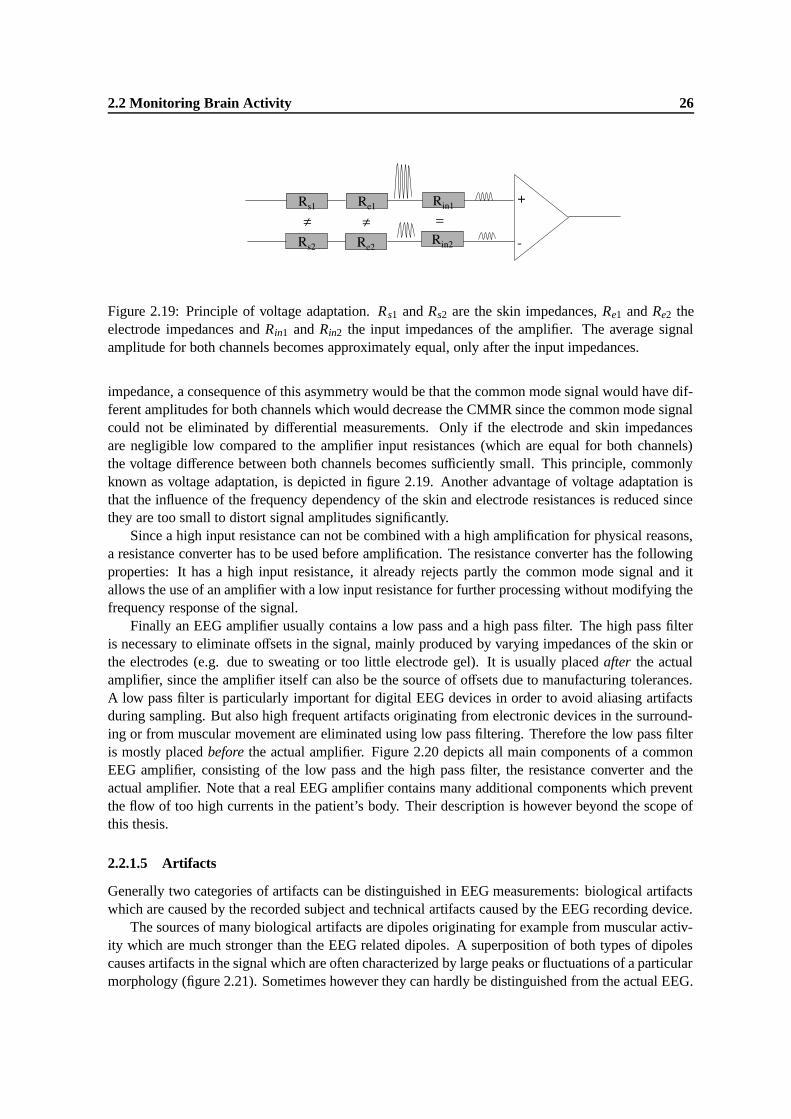
2.2 Monitoring Brain Activity 26
Figure 2.19: Principle of voltage adaptation. Rs1 and Rs2 are the skin impedances, Re1 and Re2 theelectrode impedances and Rin1 and Rin2 the input impedances of the amplifier. The average signalamplitude for both channels becomes approximately equal, only after the input impedances.
impedance, a consequence of this asymmetry would be that the common mode signal would have dif-ferent amplitudes for both channels which would decrease the CMMR since the common mode signalcould not be eliminated by differential measurements. Only if the electrode and skin impedancesare negligible low compared to the amplifier input resistances (which are equal for both channels)the voltage difference between both channels becomes sufficiently small. This principle, commonlyknown as voltage adaptation, is depicted in figure 2.19. Another advantage of voltage adaptation isthat the influence of the frequency dependency of the skin and electrode resistances is reduced sincethey are too small to distort signal amplitudes significantly.
Since a high input resistance can not be combined with a high amplification for physical reasons,a resistance converter has to be used before amplification. The resistance converter has the followingproperties: It has a high input resistance, it already rejects partly the common mode signal and itallows the use of an amplifier with a low input resistance for further processing without modifying thefrequency response of the signal.
Finally an EEG amplifier usually contains a low pass and a high pass filter. The high pass filteris necessary to eliminate offsets in the signal, mainly produced by varying impedances of the skin orthe electrodes (e.g. due to sweating or too little electrode gel). It is usually placed after the actualamplifier, since the amplifier itself can also be the source of offsets due to manufacturing tolerances.A low pass filter is particularly important for digital EEG devices in order to avoid aliasing artifactsduring sampling. But also high frequent artifacts originating from electronic devices in the surround-ing or from muscular movement are eliminated using low pass filtering. Therefore the low pass filteris mostly placed before the actual amplifier. Figure 2.20 depicts all main components of a commonEEG amplifier, consisting of the low pass and the high pass filter, the resistance converter and theactual amplifier. Note that a real EEG amplifier contains many additional components which preventthe flow of too high currents in the patient’s body. Their description is however beyond the scope ofthis thesis.
2.2.1.5 Artifacts
Generally two categories of artifacts can be distinguished in EEG measurements: biological artifactswhich are caused by the recorded subject and technical artifacts caused by the EEG recording device.
The sources of many biological artifacts are dipoles originating for example from muscular activ-ity which are much stronger than the EEG related dipoles. A superposition of both types of dipolescauses artifacts in the signal which are often characterized by large peaks or fluctuations of a particularmorphology (figure 2.21). Sometimes however they can hardly be distinguished from the actual EEG.
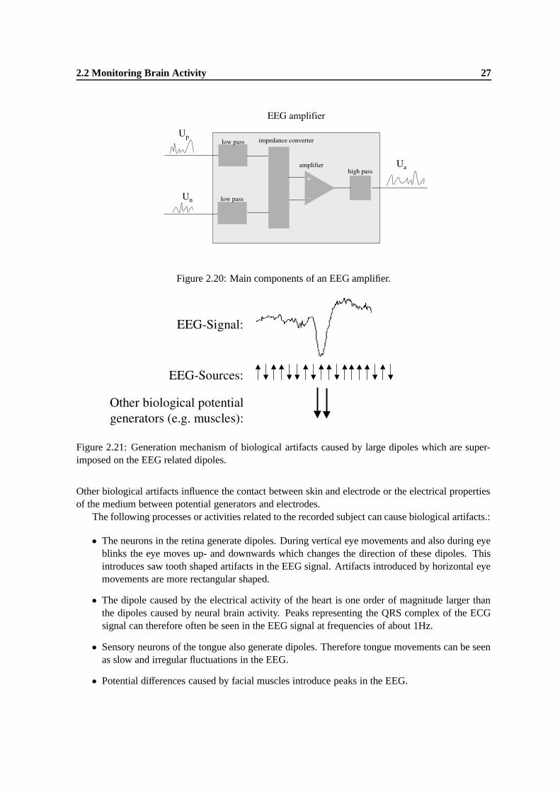
2.2 Monitoring Brain Activity 27
Figure 2.20: Main components of an EEG amplifier.
Figure 2.21: Generation mechanism of biological artifacts caused by large dipoles which are super-imposed on the EEG related dipoles.
Other biological artifacts influence the contact between skin and electrode or the electrical propertiesof the medium between potential generators and electrodes.
The following processes or activities related to the recorded subject can cause biological artifacts.:
• The neurons in the retina generate dipoles. During vertical eye movements and also during eyeblinks the eye moves up- and downwards which changes the direction of these dipoles. Thisintroduces saw tooth shaped artifacts in the EEG signal. Artifacts introduced by horizontal eyemovements are more rectangular shaped.
• The dipole caused by the electrical activity of the heart is one order of magnitude larger thanthe dipoles caused by neural brain activity. Peaks representing the QRS complex of the ECGsignal can therefore often be seen in the EEG signal at frequencies of about 1Hz.
• Sensory neurons of the tongue also generate dipoles. Therefore tongue movements can be seenas slow and irregular fluctuations in the EEG.
• Potential differences caused by facial muscles introduce peaks in the EEG.

2.2 Monitoring Brain Activity 28
• If an electrode is placed directly above a blood vessel in the scalp, its pulse changes the electricalproperties of the medium between cortex and electrode rhythmically. Furthermore it can causesmall electrode shifts. Both effects result in resistance changes between potential generator andelectrode and thus in periodic oscillations of the signal.
• The state of the subjects hair (greasy, treated with hairspray etc.) can influence resistance be-tween skin an electrode and thus cause a change of amplitudes across sessions.
• A lot of psychological and physiological effects (e.g. the increase of physical or mental task de-mand) can influence the activity of perspiratory glands resulting in resistance changes betweenskin an electrode and therefore in changes of the EEG amplitude. Note that for the assessmentfor task demand such artifacts might possibly be even of advantage.
• Sweat or too much conductive paste can cause shortcuts between electrodes which leads to astrong decrease of signal amplitudes.
The following important technical artifacts can be distinguished:
• Broken or dirty electrodes can cause sudden large potential changes, since the Helmholtz doublelayer becomes unstable.
• Dirty or corroded contacts of cables or even broken cables can cause a decrease of the signalamplitude or even a zero signal.
• Badly attached ground electrodes or a too strong asymmetry between the impedances of EEGand reference electrodes (due to dirt or corrosion) can be detrimental for the CMMR.
• Depending on the design of the amplifier noise from high frequent electromagnetic fields (e.g.radio waves) can be mapped partly to lower frequencies of the signal which are displayed in theEEG.
• Persons next to the subject which is recorded can charge themselves electrostatically. Thenelectricity which is transfered inductively to the recorded subject with large voltages can causeartifacts of variable shape in the signal.
Note that technical artifacts and also some biological artifacts can be generally avoided when therecording equipment is operated correctly and the subject to be recorded is prepared carefully. Otherartifacts are inevitable.
2.2.2 The Magnetoencephalogram (MEG)
Similar to the EEG the MEG also measures correlates of the neural brain activity. However no elec-trical potential differences but the magnetic flow caused by cortical field potentials is measured here.Since the magnetic field which corresponds to an electrical field is perpendicular to this electricalfield, the MEG is most sensitive for dipoles with a tangential orientation to the surface of the headwhile the EEG is most sensitive for dipoles which are oriented radially from the center to the surfaceof the head.
The MEG has a high temporal resolution which is comparable to the EEG and its spatial resolutionis even better. Furthermore MEG sensors require no direct contact with the skin in contrast to EEGelectrodes. The most important drawback of the MEG is however that highly sensitive magnetometers

2.2 Monitoring Brain Activity 29
(SQUIDs, i.e. super conduction quantum inference devices) must be used for its registration, since thesignals which can be measured at the scalp are extremely weak. SQUIDSs require a lot of space, theyare expensive and they must be cooled near the absolute zero temperature to exhibit their supercon-ducting properties. Therefore MEG recording with portable devices is impossible. Finally the MEGsuffers from the same problem as the EEG that only activity from a very small fraction of neurons canbe measured at the scalp (see section 2.1.2). Since EEG and MEG measure complementary signals asmentioned above, both modalities are often combined for clinical purposes.
2.2.3 Functional Near-Infrared Spectroscopy (fNIRS)
Functional Near-Infrared Spectroscopy (fNIRS) is a technique which can be used to monitor the con-centration of oxygenated hemoglobin (Oxy-Hb) and deoxygenated hemoglobin (Deoxy-Hb) in theblood. Oxy-Hb binds oxygen molecules to transport them to regions where they are consumed whileDeoxy-Hb does not bind any oxygen. Since neurons need more oxygen when more neural signalshave to be processed, the information about concentration of both hemoglobin types allows infer-ences about brain activity: A larger concentration of Oxy-Hb in a certain area indicates a higherneural activity in this area.
The underlying principle of fNIRS is that biological tissues are comparatively transparent to nearinfrared light (wavelengths between 700 and 900 nm) but hemoglobin in the blood reflects this near in-frared light at certain wavelengths. However light intensity is not only reflected but also absorbed andscattered by hemoglobin. Since the absorption and the scattering properties of Oxy-Hb and Deoxy-Hb are different, they reflect the same light impulses with different intensities. This information canbe used to calculate the relative changes of the concentration of Oxy-Hb and Deoxy-Hb at a certainposition compared to a baseline.
An apparatus for fNIRS usually consists of one or more near infrared light sources and a detectorarray. Both can easily be mounted on the forehead. Therefore fNIRS is well suited to constructportable devices for monitoring brain activity. Compared to EEG they have the advantage that noconductive paste between sensors and skin is needed, however sensors can only be placed at positionswithout hair. Furthermore the information provided by fNIRS is much less detailed than EEG data:For each sensor only an estimate of the current brain activity for the cortex region under this sensoris obtained. While this may be suitable for applications like assessment of task demand, EEG isindispensable for clinical applications since inferences about underlying neural processes can be madefrom the morphology and the frequency of the EEG signals. The temporal and spatial resolution offNIRS is comparable to EEG.
2.2.4 Functional Magnetic Resonance Imaging (fMRI)
Standard magnetic resonance imaging measures the response of biological tissue when exposed toa strong magnetic field and electromagnetic high frequency pulses perpendicular to this field. Forfunctional magnetic resonance imaging this technique is modified so that the hemodynamics relatedto neural activity in the brain can be measured.
Similar to fNIRS this monitoring technique makes use of differences between Oxy-Hb and Deoxy-Hb, which exhibit a different behavior in magnetic fields. For regions with a higher concentration ofDeoxy-Hb the fMRI response (i.e. the contrast of the obtained image) is slightly weaker comparedto regions with a higher Oxy-Hb concentration. This difference is extremely small so that in order todetect it, data obtained from several repetitions of stimuli causing a particular Oxy-Hb and Deoxy-Hb

2.2 Monitoring Brain Activity 30
distribution must be averaged (which increases the signal to noise ratio). This method is also referredto as BOLD contrast imaging, i.e. Blood Oxygen Level Dependent contrast imaging.
The precise relationship between neural signals (e.g. EEG signals) and the BOLD response isunder active research. In different studies a correlation between EEG-α activity and blood oxygenationhas been found (see for example [Laufs et al., 2003] and [Martinez-Montes et al., 2004]). Howevermodels which relate other types of neural activity to brain metabolism do not exist yet to our currentknowledge.
The temporal resolution of fMRI is much worse compared to the imaging techniques mentionedabove, since it takes 2-5 seconds to produce a single image. However a much better spatial resolutioncan be obtained: slice images are produced in a way that three dimensional models of the brain activitycan be constructed with voxels as small as three millimeters length on each side. Furthermore a lot ofbrain activity information from central brain regions can be visualized here which remains hidden toEEG, MEG or fNIRS.
An MRI device is very large and expensive and it is not suited at all to record people’s brainactivity in every-day situations. The magnetic pulses produce a lot of noise during recording and evenslight motion causes artifacts which can hardly be corrected. For clinical purposes and the study ofthe brain’s function fMRI is however well suited.
2.2.5 Single Photon Emission Computer Tomography (SPECT)
Single Photon Emission Computer Tomography (SPECT) also produces slice images of the brain,similar to fMRI. While fMRI detects however differences between oxygenated and deoxygenatedhemoglobin in the blood, SPECT provides information about the amount of blood in particular brainregions and the temporal distribution of a certain blood quantity (or a certain drug) in the brain whichhas previously been marked with radioactive tracers (radiopharmaceuticals).
The key idea of SPECT is that radiopharmaceuticals emitting gamma rays are injected in a bloodvessel prior to the examination. These radioactive tracers are transported then via cardiovascularsystem so that their concentration is particularly high at regions where more blood is required. Brainactivity has been proved to be particularly high in regions with high blood flow [Schmidt and Thews,1997], so that the gamma activity from a certain brain region can serve as indicator for activity inthis region. Note that blood flow is highly correlated with the concentration of Oxy-Hb in the blood[Schmidt and Thews, 1997] which is assessed by fNIRS and fMRI.
Gamma activity is measured using a gamma camera rotating around the patient. Thus projectionsof the gamma activity for a number of angels (usually 100-200) are obtained. Methods which arecommonly used for standard x-ray computer tomography (e.g. filtered back projection) are appliedthen to generate a slice image of the gamma activity.
The application of radiopharmaceuticals is harmful to the patient in a similar way as x-rays. There-fore SPECT can be used only for clinical applications. Furthermore the same restrictions as for fMRIconcerning the space demands of the recording unit and the mobility of the patient apply here. Thetemporal resolution of SPECT is slightly better than that of fMRI (in each second one image can beobtained), the voxels of the recorded volume however have lengths of about 1cm at each side.
2.2.6 Positron Emission Tomography (PET)
For Positron Emission Tomography (PET) radiopharmaceuticals are used which emit positrons insteadof gamma rays. Positrons are very unstable and almost immediately after emission (after a few mmpath length) a positron collides with an electron resulting in the annihilation of both particles and the

2.3 Physiological Correlates Mental States and Task Demand 31
Figure 2.22: Principal of a PET system (with modifications from [Dossel, 2000]). The coincidencedetector detects gamma quanta arriving almost simultaneously at opposite detectors. The line detectorincrements a counter for the line which connects the two detectors where the gamma quanta arrived.The values for all lines which can be interpreted as projection of the positron concentration are finallypassed to a computer for reconstruction of a slice image.
emission of two gamma quanta which move in exactly opposite directions. A detector ring around thepatient is used to detect such events, i.e. the arrival of two gamma quanta at detectors on oppositepositions of the ring at the same time (figure 2.22). For reconstruction of a slice image from thedetected events techniques similar to those used for SPECT or x-ray computer tomography are applied.
PET provides similar images as SPECT, however it has a better spatial resolution with voxels ofabout 3mm side length. However PET devices are much more expensive than SPECT devices and theproduction and application of radiopharmaceuticals is much more difficult. Their half-life period isusually only between 10min and 100min so that positron emitters must be applied almost immediatelyafter their production.
2.2.7 Summary
Table 2.1 provides an overview over all described techniques for monitoring brain activity.
2.3 Physiological Correlates Mental States and Task Demand
2.3.1 Functional Cortex Divisions and and the Identification of Mental States in theEEG
Different sensory inputs are processed at different parts of the cortex. Furthermore particular cortexareas are involved in higher mental functions such as memory, control of attention, complex planingand reasoning. Figure 2.23 gives an overview over the functions of different cortex regions.
When sensory inputs are processed or when other mental processing takes place, the correspond-ing regions of the cortex are particularly active. We are interested now in the EEG-correlates of thisactivity. At this point the thalamus becomes important. Its main role is the preprocessing of periph-eral sensory inputs and their forwarding to those cortex regions which are concerned with the finalprocessing of these inputs. These are the primary sensory cortex regions and those regions which are
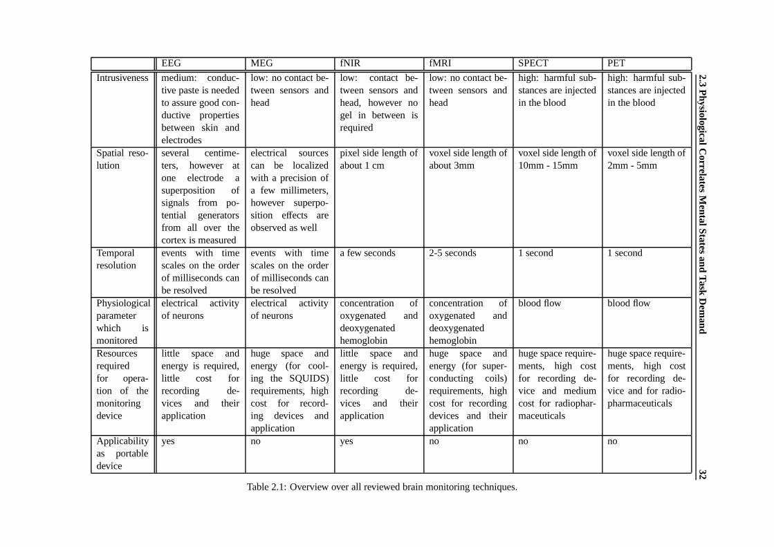
2.3P
hysiologicalCorrelates
MentalStates
andT
askD
emand
32EEG MEG fNIR fMRI SPECT PET
Intrusiveness medium: conduc-tive paste is neededto assure good con-ductive propertiesbetween skin andelectrodes
low: no contact be-tween sensors andhead
low: contact be-tween sensors andhead, however nogel in between isrequired
low: no contact be-tween sensors andhead
high: harmful sub-stances are injectedin the blood
high: harmful sub-stances are injectedin the blood
Spatial reso-lution
several centime-ters, however atone electrode asuperposition ofsignals from po-tential generatorsfrom all over thecortex is measured
electrical sourcescan be localizedwith a precision ofa few millimeters,however superpo-sition effects areobserved as well
pixel side length ofabout 1 cm
voxel side length ofabout 3mm
voxel side length of10mm - 15mm
voxel side length of2mm - 5mm
Temporalresolution
events with timescales on the orderof milliseconds canbe resolved
events with timescales on the orderof milliseconds canbe resolved
a few seconds 2-5 seconds 1 second 1 second
Physiologicalparameterwhich ismonitored
electrical activityof neurons
electrical activityof neurons
concentration ofoxygenated anddeoxygenatedhemoglobin
concentration ofoxygenated anddeoxygenatedhemoglobin
blood flow blood flow
Resourcesrequiredfor opera-tion of themonitoringdevice
little space andenergy is required,little cost forrecording de-vices and theirapplication
huge space andenergy (for cool-ing the SQUIDS)requirements, highcost for record-ing devices andapplication
little space andenergy is required,little cost forrecording de-vices and theirapplication
huge space andenergy (for super-conducting coils)requirements, highcost for recordingdevices and theirapplication
huge space require-ments, high costfor recording de-vice and mediumcost for radiophar-maceuticals
huge space require-ments, high costfor recording de-vice and for radio-pharmaceuticals
Applicabilityas portabledevice
yes no yes no no no
Table 2.1: Overview over all reviewed brain monitoring techniques.

2.3 Physiological Correlates Mental States and Task Demand 33
Figure 2.23: Functional cortex divisions according to [Schmidt and Thews, 1997] and [Dudel andBackhaus, 1996]. The cortex image is taken from [Scientific Learning Cooperation, 1999].
responsible for high level processing of the perceived information, e.g. the planning and initiation ofresponses.
The different nuclei of the thalamus can operate however in two different modes (figure 2.24),depending on the presence of sensory stimuli and on the current vigilance level:
Oscillation mode: When no or only weak sensory inputs are present for a particular nucleus and/orvigilance is low, impulses with a frequency between 8Hz and 13Hz are constantly sent to thosecortex regions where this nucleus projects to (i.e. to which this nucleus sends afferences). Theseimpulses cause a synchronization of neural activity in the corresponding cortex regions. Thusa rhythmic neural activity called α-rhythm is generated and in the EEG measured over thesecortex regions, oscillations with a frequency of the thalamus impulses can be observed.
Transfer mode: In this mode sensory inputs are preprocessed and the preprocessed information in-stead of rhythmic impulses is sent to the cortex regions which are responsible for the finalprocessing. This leads to a desynchronization of neural activity, i.e. to the attenuation or eventhe vanishing of α-activity and an increase of activity at other frequencies for the particularregions which can also be observed in the EEG.
Thus we can briefly summarize neural processes related to mental activity as follows: Given asufficiently high vigilance level and the presence of sensory inputs, the thalamic nuclei processingthese inputs switch from oscillation mode into transfer mode, i.e. they activate the correspondingcortex regions. Activation means desynchronization, so that in the EEG the power in the α-frequencyband decreases for the activated regions and power in other frequency bands increases indicating thathigher mental processes are taking place.
Note that mental activity can certainly take place as well without the presence of external sensorystimuli. Although the precise mechanisms of the cortex activation related to that kind of activity is still
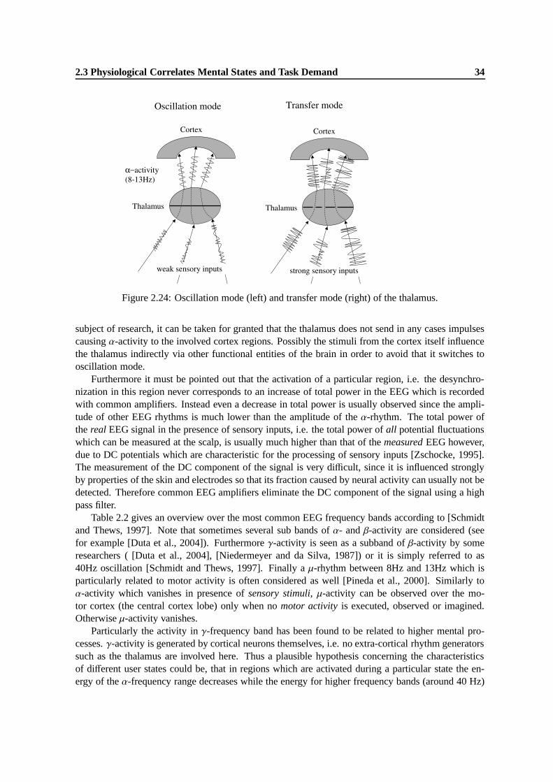
2.3 Physiological Correlates Mental States and Task Demand 34
Figure 2.24: Oscillation mode (left) and transfer mode (right) of the thalamus.
subject of research, it can be taken for granted that the thalamus does not send in any cases impulsescausing α-activity to the involved cortex regions. Possibly the stimuli from the cortex itself influencethe thalamus indirectly via other functional entities of the brain in order to avoid that it switches tooscillation mode.
Furthermore it must be pointed out that the activation of a particular region, i.e. the desynchro-nization in this region never corresponds to an increase of total power in the EEG which is recordedwith common amplifiers. Instead even a decrease in total power is usually observed since the ampli-tude of other EEG rhythms is much lower than the amplitude of the α-rhythm. The total power ofthe real EEG signal in the presence of sensory inputs, i.e. the total power of all potential fluctuationswhich can be measured at the scalp, is usually much higher than that of the measured EEG however,due to DC potentials which are characteristic for the processing of sensory inputs [Zschocke, 1995].The measurement of the DC component of the signal is very difficult, since it is influenced stronglyby properties of the skin and electrodes so that its fraction caused by neural activity can usually not bedetected. Therefore common EEG amplifiers eliminate the DC component of the signal using a highpass filter.
Table 2.2 gives an overview over the most common EEG frequency bands according to [Schmidtand Thews, 1997]. Note that sometimes several sub bands of α- and β-activity are considered (seefor example [Duta et al., 2004]). Furthermore γ-activity is seen as a subband of β-activity by someresearchers ( [Duta et al., 2004], [Niedermeyer and da Silva, 1987]) or it is simply referred to as40Hz oscillation [Schmidt and Thews, 1997]. Finally a µ-rhythm between 8Hz and 13Hz which isparticularly related to motor activity is often considered as well [Pineda et al., 2000]. Similarly toα-activity which vanishes in presence of sensory stimuli, µ-activity can be observed over the mo-tor cortex (the central cortex lobe) only when no motor activity is executed, observed or imagined.Otherwise µ-activity vanishes.
Particularly the activity in γ-frequency band has been found to be related to higher mental pro-cesses. γ-activity is generated by cortical neurons themselves, i.e. no extra-cortical rhythm generatorssuch as the thalamus are involved here. Thus a plausible hypothesis concerning the characteristicsof different user states could be, that in regions which are activated during a particular state the en-ergy of the α-frequency range decreases while the energy for higher frequency bands (around 40 Hz)

2.3 Physiological Correlates Mental States and Task Demand 35
Name Frequency range
δ 0.5Hz - 3.5Hzθ 4Hz - 7Hzα 8Hz - 13Hzβ 14Hz - 30Hzγ around 40Hz
Table 2.2: Different EEG frequency bands according to [Schmidt and Thews, 1997]
increases.Figure 2.25 shows the spectrograms for 16 electrodes for recordings of the user states resting,
listening to a talk and reading an article in a magazine. While spectrograms of single electrodes oftendo not differ much across all three or at least two of these user states, the information contained inthe spectrograms of all electrodes seems sufficient to uniquely identify a particular state. This seemseven possible when pooling frequencies into only two sub-bands, a lower and higher one. In somecases the differences between the spectrograms across states can be explained by the fact that regionswhich should be activated during a particular state (according to figure 2.23) show an increase ofhigh frequencies and a decrease of low frequencies: Electrode P4 (which is located over the parietalcortex, see figure 2.12) shows for example much more high frequent activity during reading thanduring resting or listening. However this hypothesis is by far not true in all cases. Electrode T4for example should capture activity from the areas in the temporal cortex which process speech andlanguage. However, it shows more high frequent activity during resting than during the other states.
We conclude that for different mental states different kinds of potential fluctuations over the wholecortex can be observed, i.e. the frequency content of the signals measured at several electrodes dif-fers. The combination of the spectrograms obtained for the signals from all these electrodes resultsin a pattern which can identify a user state uniquely. While it is probably difficult to explain the pat-tern corresponding to a particular state by a priori knowledge, the information that different patternsfor different states exist, seems sufficient to attempt the application of statistical machine learningalgorithms for their discrimination.
2.3.2 Task Demand, Alertness and Vigilance
In psychology and ergonomics the distinction between task demand (stress) and workload (strain) isvery important. Mental task demand is defined as the degree to which an individual has to use hismental resources to fulfill a certain task while mental workload corresponds to the complexity of atask independent from the mental resources required by an individual for its execution [Bokranz andLandau, 1991].
Within this thesis we are concerned with the assessment of mental task demand, i.e. we areinterested in the effect which a mental task has on an individual. This is often, but not necessarilycorrelated with the complexity of the task itself, i.e. with workload.
The relationship between the physiological correlates of task demand and workload (i.e. taskcomplexity) has been analyzed in many research works, e.g. [Smith et al., 2001,Pleydell-Pearce et al.,2003, Berka et al., 2004, Izzetoglu et al., 2004]. (These works are reviewed in section 3.2 in greaterdetail.) For this purpose physiological data (e.g. EEG, EMG, ECG etc.) was collected during theexecution of tasks which varied in difficulty (i.e. tasks with varying workload), and regression func-tions were trained to output indices representing the use of mental resources during task execution. Inall cases data points from different workload levels were used as examples for different task demand
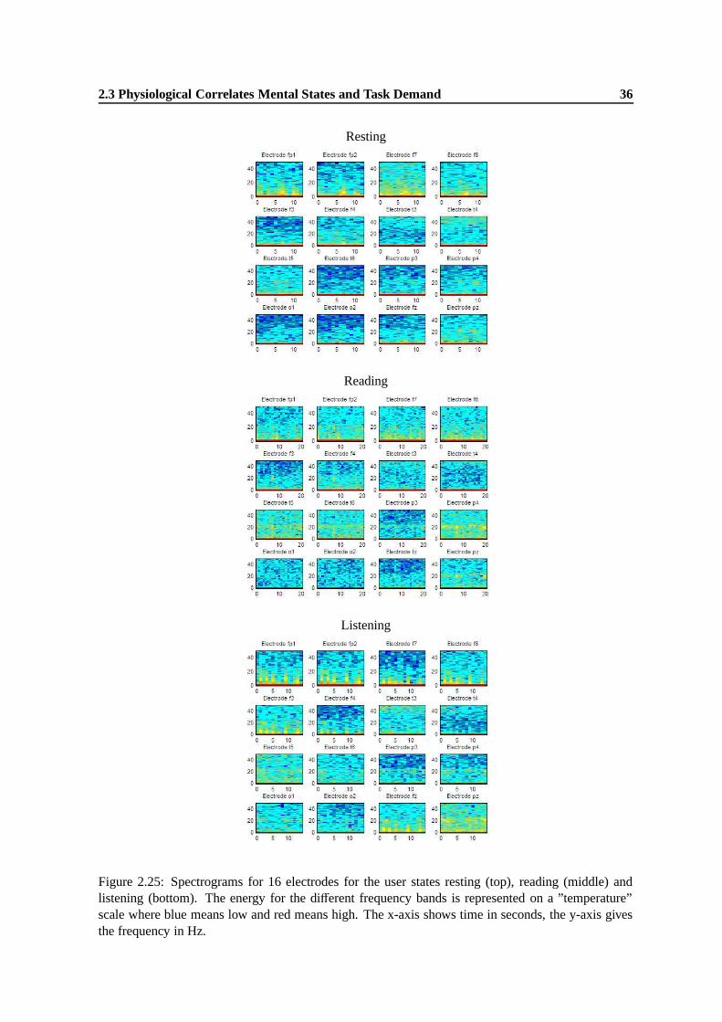
2.3 Physiological Correlates Mental States and Task Demand 36
Resting
Reading
Listening
Figure 2.25: Spectrograms for 16 electrodes for the user states resting (top), reading (middle) andlistening (bottom). The energy for the different frequency bands is represented on a ”temperature”scale where blue means low and red means high. The x-axis shows time in seconds, the y-axis givesthe frequency in Hz.
2.3 Physiological Correlates Mental States and Task Demand 37
levels, relying on the assumption that both parameters are correlated. (Often authors even use theterms workload or task load to characterize the use of mental resources, i.e. task demand according toour definition.)
In [Jung et al., 1997] and [Duta et al., 2004] (see section 3.2 for more details on these works)natural fluctuations of the availability of mental resources during tasks requiring sustained attentionwas examined, while workload was kept constantly. These fluctuations are commonly referred tochanges in alertness or vigilance (see below). In [Duta et al., 2004] EEG data segments for differentvigilance levels were obtained by manual annotation of the data, while in [Jung et al., 1997] the rateof failures to respond correctly to given stimuli was used as an indicator of vigilance. In both worksalso regression functions are trained which output an index reflecting the use of mental resources.
The performance of the different regression functions representing either task demand or alert-ness/vigilance was evaluated by correlating their outputs with different measures: [Berka et al., 2004,Izzetoglu et al., 2004] used the difficulty levels (i.e. the workload levels) of the performed task as ref-erences, [Pleydell-Pearce et al., 2003,Berka et al., 2004,Izzetoglu et al., 2004,Smith et al., 2001,Junget al., 1997] an error measure or a performance measure which are both functions of failures to givecorrect responses to certain stimuli, [Duta et al., 2004] an expert rating of vigilance obtained by visualinspection of the EEG and [Smith et al., 2001] self-estimations of task demand.
We conclude that it seems difficult (or even impossible) to obtain objective measures for the useof mental resources which can be used to develop an EEG-based task demand index. Either one hasto rely on subjective estimations of task demand, or task demand must be estimated indirectly relyingon the hypothesis that it is well correlated with other parameters. (For some physiological parameterssuch as ECG or EEG this correlation is proved to be rather strong.)
While the terms alertness (in its common sense meaning) and vigilance can be treated as synonymsfor this work, their relation to task demand needs some explanation.
Vigilance is defined as a physiological continuum which ranges from fully responsive (also re-ferred to as active alertness) to sleepiness [Zschocke, 1995]. In the state of high vigilance sufficientmental resources are available and these resources are used either to process a huge number of stim-uli or to expect stimuli attentively. Vigilance decreases either when less mental resources becomeavailable (because the individual is not relaxed but sleepy), while the amount of stimuli may remainconstant, or when the number of stimuli decreases and/or they are expected with less attention. Notethat stimuli can be either ”external” sensory stimuli, or ”internal” stimuli. The latter denote puremental processes such as complex reasoning.
Since mental task demand is defined, according to our definition, as the amount of mental re-sources which are required for the execution of a specific task, we hypothesize the following relationbetween task demand and vigilance: In situations of high task demand a large amount of mental re-sources is required since there are many ”external” or ”internal” stimuli to be processed. That meansthat for a relaxed individual vigilance is high as well. When task demand is reduced, the number ofstimuli decreases which means according to the above explanation a decrease of vigilance. Only if anindividual is not relaxed, vigilance level and task demand level can be different, since it may happenin such cases that many mental resources are required but not available. Note that sometimes the termvigilance is even used to characterize task demand. In [Berka et al., 2004] a developed task demandindex is called a vigilance index for example.
In the next section neural and EEG correlates of vigilance are described according to [Zschocke,1995]. These should be correlates of task demand as well following the above hypothesis. Further-more spectrograms from EEG data recorded for this work are shown, which confirm this hypothesis,since for different task demand levels they exhibit EEG characteristics corresponding to different vig-ilance levels. Finally some non-EEG correlates of task demand are enumerated.

2.3 Physiological Correlates Mental States and Task Demand 38
2.3.2.1 Physiological Correlates of Vigilance and Task Demand
The formatio reticularis plays a crucial role for the regulation of vigilance [Zschocke, 1995]. Thisanatomical structure contains the ascending reticular activating system (ARAS) which controls (viathe thalamus) the brain’s α-activity. In a state of high vigilance (fully responsiveness or active alert-ness) α-activity decreases and desynchronization can be observed which is mostly connected with acortex activity at higher frequencies which can be seen in the EEG.
This effect has already been explained in section 2.3.1 with the change of the operation modeof the thalamus (from oscillation mode to transfer mode). Reasons for this operation mode changeare not exclusively the presence of sensory stimuli but also changes in vigilance level have a certaininfluence. In states of high vigilance the ARAS sends afferences to the thalamus so that its nucleiswitch much easier into transfer mode (even when little stimuli are present). This causes that sensoryinputs are transmitted more strongly (with higher impulse rate) to the cortex and that less nucleiremain in oscillation mode, so that less α-activity and more desynchronization can be observed allover the cortex. Additionally during states of high vigilance the ARAS makes the thalamus nucleisend afferences to cortex regions which are not primarily concerned with the processing of sensoryinputs (diffuse projection) but which are responsible for higher mental processes and the high levelprocessing of sensory inputs.
Thus the degree of vigilance is correlated correlated positively with the amplitude of non-α-activity and negatively with the amplitude of α-activity. If the reason for high vigilance is the ex-ecution of a particular mental task, such as complex reasoning to understand a talk or a presentation,especially an increase of 40Hz activity is to be expected, which is most pronounced in those regionswhich are mainly concerned with the required processing (see also section 2.3.1). In analogy to that,the amplitude of the α-frequency band is expected to decrease mostly in these regions, but it shouldbe attenuated in other regions as well. For a relaxed individuals we hypothesize to observe the samephenomena when the level of task demand changes for the reasons explained above.
Based on the above explanations, the relation between the neural correlates of task demand anddifferent user states shall finally be summarized briefly: In section 2.3.1 is has been explained, thatduring each user state different cortex regions are activated, i.e. a desynchronization (increase ofnon-α-activity and decrease of α-activity) can be observed. The degree of desynchronization in theseregions is directly correlated with the degree of task demand.
Figure 2.26 shows the spectrograms for EEG signals of 16 electrodes recorded during periodslow task demand and high task demand of subjects who perceived a slides presentation. For manyelectrodes it can be seen that there is more high frequent activity for high task demand compared tolow task demand. For other electrodes the contrary is the case however, for example for electrodesPz or Fp2. A possible explanation for this could be that one or a few subtasks required more mentalresources when the overall task demand was rated to be low, compared to the case where the subjectrated his overall task demand to be high. Nevertheless the hypothesis seems to hold that in generalan increase of high frequent activity corresponds to an increase of task demand. The decrease oflower frequent activity for high task demand is very small, i.e. the amplitude of the α-activity seemsto be attenuated only little. This is however not too surprising, since even in situations of low taskdemand already enough stimuli are present so that only little α-activity remains. The high amplitudeof the lower frequency bands is not only explained with α-activity, but also with artifacts (see inparticular the red columns in the spectrograms of the prefrontal and frontal electrodes in case of lowtask demand) and with other EEG activity (e.g. θ-activity and δ-activity, see table 2.2). Note thatduring the perception of a presentation virtually all cortex regions are involved: the temporal cortexfor the understanding of speech, the temporal and parietal cortex for the understanding of slides,

2.3 Physiological Correlates Mental States and Task Demand 39
LowElectrode fp1
0 2 4 6 80
20
40
Electrode fp2
0 2 4 6 80
20
40
Electrode f7
0 2 4 6 80
20
40
Electrode f8
0 2 4 6 80
20
40
Electrode f3
0 2 4 6 80
20
40
Electrode f4
0 2 4 6 80
20
40
Electrode t3
0 2 4 6 80
20
40
Electrode t4
0 2 4 6 80
20
40
Electrode t5
0 2 4 6 80
20
40
Electrode t6
0 2 4 6 80
20
40
Electrode p3
0 2 4 6 80
20
40
Electrode p4
0 2 4 6 80
20
40
Electrode o1
0 2 4 6 80
20
40
Electrode o2
0 2 4 6 80
20
40
Electrode fz
0 2 4 6 80
20
40
Electrode pz
0 2 4 6 80
20
40
HighElectrode fp1
0 2 4 6 80
20
40
Electrode fp2
0 2 4 6 80
20
40
Electrode f7
0 2 4 6 80
20
40
Electrode f8
0 2 4 6 80
20
40
Electrode f3
0 2 4 6 80
20
40
Electrode f4
0 2 4 6 80
20
40
Electrode t3
0 2 4 6 80
20
40
Electrode t4
0 2 4 6 80
20
40
Electrode t5
0 2 4 6 80
20
40
Electrode t6
0 2 4 6 80
20
40
Electrode p3
0 2 4 6 80
20
40
Electrode p4
0 2 4 6 80
20
40
Electrode o1
0 2 4 6 80
20
40
Electrode o2
0 2 4 6 80
20
40
Electrode fz
0 2 4 6 80
20
40
Electrode pz
0 2 4 6 80
20
40
Figure 2.26: Spectrograms for 16 electrodes for low (top) and high (bottom) task demand duringlistening to a talk. The energy for the different frequency bands is represented on a ”temperature”scale where blue means low and red means high. The x-axis shows time in seconds, the y-axis givesthe frequency in Hz.
the occipital cortex for visual perception and the frontal cortex for the control of attention. Thereforedifferences in the frequency content of the EEG signals for the different task demand levels can be seenfor electrodes at positions all over the cortex. We conclude that the observations from the spectrogramsconfirm the hypothesis that EEG correlates of task demand and vigilance are closely related.
An increase of vigilance and task demand is also characterized by an increasing amount of oxy-genated blood forehead, i.e. more oxygen is transported in the blood. For overload a decrease of bloodoxygenation compared to the highest oxygenation level can be observed [Izzetoglu et al., 2004]. Fur-thermore the magnitude of pupil dilation has been shown to be a function of mental effort which isrequired to perform a cognitive task [Beatty, 1982], [Hoecks and Levelt, 1993].

Chapter 3
Related Work
A lot of research is concerned with the computational processing of human brain activity with non-clinical purpose. In most cases EEG is used for data recording but also functional magnetic resonancetomography (fMRI) and functional near infrared spectroscopy (fNIRS) are applicable techniques forphysiological data acquisition. Three main research goals can be distinguished:
1. Identification of different mental states, i.e. different mental activities. These activities canbe very different such as resting vs. performing mental arithmetic or very similar such as theperception of different word categories (e.g. fish vs. for-legged-animals vs. trees vs. flowers).
Different motivations exist for this research goal: Human cognition can be studied by analyzingthe properties of classifiers which discriminate mental states [Mitchell et al., 2004], i.e. infer-ences about the effect of different mental states on neural activity can be made. Furthermore theknowledge about states which can be discriminated particularly well and about methods whichare suitable for that is an important preparatory work for the development of Brain-Computer-Interfaces (BCIs), which attempt to control electronic devices using only brain activity. Notethat we distinguish the research which is concerned with the shear discrimination of mentalstates (mostly but not exclusively for BCI purposes, [Anderson et al., 1995, Anderson and Si-jercic, 1996, Ford, 1996, Culpepper, 1999]) from the actual construction of BCIs (see item 3),where also the closed-loop feedback is an essential component [Lethonen, 2003] (see also sec-tion 3.3). Finally the development of intelligent user interfaces [Chen and Vertegaal, 2004] isto be mentioned as a motivation for the identification of different mental (and physical) states.
2. Assessment of mental task demand, alertness or vigilance (see section 2.3.2 for a detailed de-scription of these terms). In most experimental setups of the works pursuing this research goalone single task was performed for which the difficulty was varied in order to provoke differentlevels of task demand of the recorded subject. Other researchers made experiments where thetask difficulty stayed constantly but a task requiring sustained attention had to be executed fora longer period of time. From the physiological data recorded during task execution it was at-tempted to predict natural fluctuations of vigilance. Because we hypothesize a close connectionbetween task demand and vigilance which has been explained in section 2.3.2, we summarizethe research which is concerned with either of these parameters in this category.
Two primary reasons for the assessment of task demand, alertness of vigilance can be distin-guished: During critical tasks it is important to be able to predict and to avoid mental overloadand too low alertness in order to prevent dangerous situations [Smith et al., 2001, Pleydell-Pearce et al., 2003, Duta et al., 2004]. Furthermore operator performance can be increased,

3.1 Identification of Mental States 41
when it is possible to maintain the operator’s cognitive load on an optimal level by adapting theway data is presented appropriately [Jung et al., 1997,Berka et al., 2004, Izzetoglu et al., 2004].A lot of the research which follows this motivation for task demand estimation has been donein a military context, namely for the DARPA Augmented Cognition Program [Schmorrow andKruse, 2002].
3. Brain-Computer-Interfaces (BCIs). As mentioned above, the goal of BCIs is to give commandsto electronic devices using only brain activity. Prominent examples for BCIs are systems tocontrol prostheses or to allow locked-in patients to communicate although they are no longercapable of voluntary movements.
3.1 Identification of Mental States
In the past decade a lot of work aiming at the identification of mental states has been done whichused the data set recorded by Keirn and Aunon [Keirn and Aunon, 1990]. This dataset consistsof EEG data recorded at the electrode positions O1, O2, P3, P4, C3, C4 (see figure 2.12 for theprecise positions) and an additional EOG channel for artifact detection. The data was recorded with asampling frequency of 250 Hz and the following tasks were performed during EEG recording:
Baseline – Alpha Wave Production: Subjects were asked to relax and to close and open their eyesin five seconds intervals. Doing this, α-activity can be observed, at least when eyes are closed.
Mental Arithmetic: Subjects had to solve non-trivial multiplications without vocalizing or moving.
Geometric Figure Rotation: Subjects were shown a drawing of a complex geometric figure. Thenthe figure was moved out of sight and subjects were instructed to imagine the rotation of thisfigure.
Mental Letter Composing: Subjects were instructed to mentally compose a letter to a friend or rel-ative, without moving or vocalizing.
Visual Counting: Subjects had to imagine a black board and mentally to visualize numbers beingsequentially written on the board.
Note that these kinds of tasks are not very likely to occur in every day situations in contrast tothe activities which are considered in this work (see section 1.1). However the focus of the researchin [Keirn and Aunon, 1990] was rather to reliably discriminate different mental states to be able togive commands to a computer then to discriminate user states.
In [Anderson et al., 1995], [Anderson and Sijercic, 1996], [Ford, 1996] the data set describedabove is used to train and test systems for the discrimination of mental states. In [Culpepper, 1999]data for the same tasks was recorded for one subject, using the electrodes FPz, F3, Fz, F4, FCz, C3,Cz, C4, Pz, P3 and P4 and an additional EOG channel.
To allow an easy comparison of the mentioned research works, the used data portions, the appliedmethods and obtained results are summarized below using a common scheme.

3.1 Identification of Mental States 42
Author: [Anderson et al., 1995]
Considered mental states: Baseline task, arithmetic task
Used Data: Two recording sessions of one subject, 10 trials per task from both sessions. From 790quarter second long patterns per task 80% are used for training, 10% for validation and testingrespectively. The data for each set is randomly chosen from both recording sessions. 10-foldcross-validation is performed.
Methods:
Artifact Removal: none
Feature Extraction: Three representations of quarter second long time segments are investi-gated: unprocessed time signals, a reduced dimensional representation obtained using theKarhunen-Loeve transform, a frequency spectrum based representation estimated with asixth-order auto regressive (AR) model.
Classification: Feed forward two-layer neural networks with up to 40 neurons in the hiddenlayer
Results: An accuracy of 74% for the discrimination of both states is obtained using the frequencyspectrum based data representation.
Authors: [Anderson and Sijercic, 1996]
Considered mental states: All five states described above
Used Data: Data from four subjects, two recording sessions per subject, 10 trials per task and sub-ject over both sessions. 277 half second long patterns per task and subject are available, afterdiscarding eye blinks. Training set size: 80% of the whole data, validation and test set sizerespectively: 10% of the whole data. The data for each set is randomly chosen from bothrecording sessions. 10-fold cross-validation is performed.
Methods:
Artifact Removal: Time segments containing eye blinks are discarded using information fromthe EOG channel.
Feature Extraction: All six coefficients of a sixth-order autoregressive model for each elec-trode are used, resulting in a total feature vector dimensionality of 36.
Classification: Feed forward two-layer neural networks with 20 neurons in the hidden layer
Results: An average accuracy of 54% in subject dependent experiments is obtained when averagingover the network outputs for 20 consecutive half second long time segments.

3.1 Identification of Mental States 43
Author: [Ford, 1996]
Considered mental states: Baseline task, arithmetic task
Used Data: Data from four subjects, two recording sessions per subject, 10 trials per task and sub-ject over both sessions. 241 half second long patterns per task and subject are available, afterdiscarding eye blinks and balancing the data set. Training set size: 80% of the whole data,validation and test set size respectively: 10% of the whole data. 10-fold cross-validation isperformed.
Methods:
Artifact Removal: Time segments containing eye blinks are discarded using information fromthe EOG channel.
Feature Extraction: All six coefficients of a sixth-order autoregressive model for each elec-trode are used, resulting in a total feature vector dimensionality of 36.
Classification: Learning Vector Quantization
Results: In session and subject dependent experiments and average accuracy of 73% is obtained.Mixing of data from both sessions for each subject yields in an average accuracy of 85.5%.
Author: [Culpepper, 1999]
Considered mental states: All five states described above; only different triplets and pairs are con-sidered for discrimination.
Used Data: Two recording sessions from one subject, 10 trials per task over both sessions. From200 half second long time segments per task 50% are used for training and 50% for testing andvalidation.
Methods:
Artifact Removal: Independent component analysis is applied to the data to isolate eye blinksto one component. This component is identified by visual inspection and then rejected.
Feature Extraction: A frequency representation of half second long to 120 second long seg-
ments of the independent components is obtained using a discrete Fourier transform.
Classification: Three-layer feed forward neural networks with 40 to 1000 neurons in the firstand 5 to 100 neurons in the second hidden layer
Results: Classification accuracies for best discriminated task pairs (results for other pairs are notreported): 94% figure rotation vs. arithmetics, 90% for baseline vs. letter composition, 82% forbaseline vs. countingClassification accuracies for best discriminated task triplets (results for other triplets are notreported): 86% for baseline vs. letter composition vs. arithmetics, 77% for counting vs. figurerotation vs. letter composition, 74% for letter composition vs. figure rotation vs. artihmetics
One important conclusion to be drawn from the above presented research works is that the dis-crimination of mental states using EEG data is possible in general. Furthermore statistical learning

3.1 Identification of Mental States 44
methods such as neural networks and a representation of the EEG signals in frequency domain seemto be suitable for this task.
More recently other work concerning the discrimination of mental states has been done, whichdoes not rely exclusively or not at all on EEG data.
[Chen and Vertegaal, 2004] proposed a physiologically attentive user interface (PAUI) which isable to distinguish four user states which are defined by the current level of mental and motor activity:”resting” (low mental activity, no movement), ”moving” (low mental activity, sustained movement),”thinking” (high mental activity, no movement) and ”busy” (high mental activity, sustained move-ment). The mental activity level is estimated using heart rate variability, the degree of motor activityis determined using EEG data from one electrode over the central cortex where motor activity is con-trolled1 . Spectral analysis of the heart rate variance is applied to detect increases of mental load whichis characterized by increasing heart rate variance. The onset of motor activity and thus a user statechange is detected by the decrease in power for the µ-frequency band (see section 2.3.1) in the EEG .
For each state the cost for different kinds of interruptions by a mobile device is defined: Whilethis cost is low for all kinds of interruptions during resting, it is low during moving for speech-related events only (e.g. for answering a phone call, since no additional complex movements must bemade for that), but high for events which require complex motor activity such as responding to a textmessage or a chat request. For the user state thinking only non-auditory interruptions (i.e. vibrations,visual notifications) are defined to be acceptable, i.e. they have a low cost, since audible alerts wouldpotentially interfere with mental engagement according to the authors. For the state busy the cost forall kinds of interruptions is set to be high. As a sample application a cell phone has been augmentedwith user state detection capabilities and in a six person trial the correct user state could be identifiedin 83% of all cases.
[Mitchell et al., 2004] use fMRI data to discriminate mental states like looking at a picture vs.reading a sentence describing that picture, reading a non-ambiguous sentence vs. reading an ambigu-ous sentence or hearing words from different categories (food, people, buildings etc.). Note that theconsidered states seem to be little different from each other compared to those considered in [Keirnand Aunon, 1990] or to states like reading, perceiving a presentation, resting etc. with which we areconcerned in this work. Since fMRI data provides a much better spatial resolution and thus a muchbetter insight into brain activity than EEG data, the discrimination of very similar states becomes morerealistic.
For each set of mental states data from five to fifteen subjects is used. Motion artifacts are re-moved from the data and several seconds long time segments of data consisting of activity values foreach voxel (i.e. for each cubic volume element of the recorded three dimensional data) are used asinput features for different classifiers. Activity values are given as deviation from the mean activitymeasured during a resting condition. The performance of Gaussian Naive Bayes classifiers, SupportVector Machines and k-nearest neighbor classifiers is investigated. Since very high dimensional fea-ture vectors are obtained from fMRI data, two different methods for feature reduction are explored.The first method attempts to select those features which discriminate the states to be distinguishedbest. This is done by training one classifier separately for each feature which uses this features onlyto make predictions. Then those features are selected for which the classifiers yield the best clas-sification accuracies. In contrast to that the second method selects those voxels as features havingthe best signal-to-noise ratio. Such features have the property that they discriminate best between
1Note that this approach does not agree with the intuition that mental activity would be estimated best with EEG dataand motor activity via the heart rate. It has been shown however that there is a correlation between mental load and the heartrate variability and between the degree of motor activity and the EEG of the µ-frequency band (see [Chen and Vertegaal,2004] for appropriate references).

3.2 Assessment of Task Demand, Vigilance or Alertness 45
a resting condition and an activity condition under which all states to be actually discriminated aresummarized. The second method is shown to outperform the first one in many cases.
Results are reported in terms of normalized rank error which considers the rank the classifiersassign to the correct hypothesis. It ranges from 0 when the correct class is ranked most likely, to 1when it is ranked least likely. Using Gaussian Naive Bayes classifiers and Support Vector Machines,average normalized rank errors between 0.11 and 0.24 are reported for subject specific experiments.For the picture vs. sentence study classifiers are trained across subjects as well. Using support vectormachines a normalized rank error of 0.25 is reported for these experiments.
Some findings from this research are also interesting for the computational processing of EEGdata, since in both cases the problem of data sparseness paired with a high feature vector dimension-ality has to be addressed:
• With linear Support Vector Machines at least comparable or even better classification resultscan be obtained compared to non-linear classifiers (such as k-Nearest Neighbors or GaussianNaive Bayes classifiers), when the dimensionality of the feature space is high.
• For noisy data the selection of features which discriminate a baseline condition from all otherconditions can improve classification results, since the signal-to-noise ratio is improved.
• There are similarities in the neural correlates of different mental states across subjects, so thattraining of subject independent classifiers for the discrimination of these states becomes possi-ble.
3.2 Assessment of Task Demand, Vigilance or Alertness
A lot of research in the domain of task demand, vigilance or alertness assessment during the executionof tasks requiring sustained attention has been done in recent years. To provide a better overview overthe research works reviewed in this section and to allow their comparison, the most important aspectsof each work are summarized below using a common scheme.
Authors: [Jung et al., 1997]
Goal: Estimation alertness during a sustained attention task.
Task: Subjects have to respond to auditory stimuli. The task should simulate sonar target detection.
Electrodes: 5 electrodes from central, parietal and occipital cortex are used.
Amount of data: In three recording sessions lasting 28 minutes 10 subjects were recorded. Onesession is used for training, validation and testing respectively. 967 time segments of 1.6slength are extracted from each session.
Methods:
Artifact removal: Signals exceeding a certain threshold are discarded as artifactual data. Me-dian filtering is used to further minimize the presence of artifacts.
Features: The log spectral power for 81 frequency bands between 0.5Hz and 50Hz is com-puted. Then principal component analysis is applied and the four principal componentscovering most variance of the data are retained.
Prediction method: Feed forward neural networks with 3 neurons in one hidden layer andmultivariate linear regression functions are used to predict an alertness index which is afunction of failures to respond to the given stimuli residing in [0, 1].

3.2 Assessment of Task Demand, Vigilance or Alertness 46
Results: An RMS-Error between classifier prediction and the alertness index of 0.163 for linear re-gression and 0.156 for neural networks is reported. All results are obtained in session indepen-dent but subject dependent experiments.
Authors: [Smith et al., 2001]
Goal: Monitoring of subject specific task loading
Task: The MATB task is used which simulates activities of a pilot: systems monitoring, resourcemanagement, communication and tracking. The subjects must react with keyboard inputs onchanges of gauges, warning lights and auditory stimuli. A joystick is used for the tracking taskwhich simulates manual control of the aircraft position. Task difficulty is varied from passivewatching to high load. Note that the variation of task difficulty showed a significant correlationwith a subjective rating (NASA Task Load Index) performed by the recorded subjects.
Electrodes: Afz, Fz, F3, F4, Fz, P3, P4, Pz
Amount of data: For 16 subjects three session were recorded, each load level (passive watching,low, medium, high) was simulated for five minutes per session. One session is used for training,validation and test respectively.
Methods:
Artifact removal: Adaptive filtering techniques are applied for artifact removal.
Features: Spectral power is estimated for several sub-bands of alpha (8-13Hz) and theta (4-7Hz) frequency ranges for four seconds long time segments.
Prediction method: Subject-specific multivariate distance functions are estimated using datafrom load levels passive watching and high load. These functions compute a subject-specific task load index between 0 (passive watching) and 1 (high task load).
Results: For subject specific but session independent experiments, significant correlations betweensubjective task difficulty ratings and results of the estimated task load predictors or betweenreaction times on stimuli and results of the task load predictors can be found. Furthermoresignificantly higher task loads are predicted for load level high compared to load level low for15 out of 16 subjects. Significant differences in predictions for low vs. moderate task load orhigh vs. moderate task load are observed only for half of the recorded subjects.
Authors: [Pleydell-Pearce et al., 2003]
Goal: Prediction of task load, investigation whether different predictors are suited for different sub-jects.
Task: Gauge monitoring task: Pushbuttons and a joystick are used to maintain changing gauges at acertain level. Task difficulty is varied by varying the tendency of the actual gauge value to moveaway from the optimal value. Performance is measured as deviation of the gauges’ currentvalues from their optimal values. All performance measurements for each subject are sortedand then split by the median so that finally only low and high task performance is distinguished.

3.2 Assessment of Task Demand, Vigilance or Alertness 47
Electrodes: Fp1, Fp2, Fpz, F7, F8, Fz, Cz, T5, T6, P3, P4, Pz, O1, O2 and vertical and horizontalEOG
Amount of data: Six subjects participated in two recording sessions. During each session each offive difficulty levels was simulated 10 times. Each time 40 seconds of data were recorded. Thisresults in 33 minutes of data per subject.
Methods:
Artifact removal: Artifacts are removed using information from the EOG channel.
Features: 5166 dependent variables are computed for 10 second long time segments. Featuresinclude string length, mean area under the curve of the time signals, inter-electrode coher-ence, cross phase and cross power correlation between electrodes and spectral power forselected frequency bands between 0Hz and 100Hz. The features which are correlated bestwith task performance are then selected to be included in the prediction functions.
Prediction method: A multivariate linear regression model is used for prediction of task per-formance (not of the task difficulty). The underlying hypothesis here is that worse taskperformance indicates higher task load which is more challenging and stressful for a sub-ject and therefore should have correlates in the EEG.
Results: Accuracies of 71.9% for the discrimination of low and high performance averaged over allsix subjects in session dependent and 70.8% in session independent experiments are reported.For subject independent experiments an accuracy of 71.0% is obtained.
Remarks: Different features are found to be the best predictors for different subjects. Therefore theauthors conclude that idiosyncratic aspects of EEG patterns reflect genuine and reproducibledifferences between subjects. Some predictors could be identified however which are validfor all subjects and it can be seen from the results that they work well for predictions acrosssubjects.
Authors: [Duta et al., 2004]
Goal: Estimation of alertness during a sustained attention task.
Tasks: Tracking a position indicator on a computer screen, reacting to a visual stimulus, keepingthe value of a continuously changing gauge at zero. The subjects’ vigilance during the taskswas rated by experts who manually labeled 15 seconds long segments of the signals using aseven-class alertness classification system.
Electrodes: A1, A2 (mastoid EEG)
Amount of data: Approximately two hours of data for each of eight subjects was collected. In around robin manner data from one subject is used for test, while training and validation isperformed on the data from the remaining subjects.
Methods:
Artifact removal: Artifacts are detected by visual inspection of the raw data and discarded.
Features: The coefficients of fifth order AR models which estimate the power spectrum in arange between 0Hz and 30Hz for 1 second long time segments for each electrode channelare used as features.

3.2 Assessment of Task Demand, Vigilance or Alertness 48
Prediction method: A feed forward two-layer neural network with 10 neurons in the hiddenlayer is used to estimate a regression function which predicts alertness. Outputs are thengrouped in three classes (alertness, intermediate, drowsiness) using thresholding
Results: Accuracies for the comparison with expert labels range between 39% and 62% for subjectindependent experiments.
Remarks: An interesting method for data analysis is applied here. This is necessary since the man-ually labeled segments have a length of 15 seconds but only one second long time segmentsare used for computational processing. Thus it is possible that some of the one second longsegments have wrong labels. Self-organizing maps are trained here to cluster all data points ofthe training data. Then those data points are removed which are mapped in the same areas asother data points belonging a different alertness category.Another interesting aspect of this work is that only electrodes at the mastoids are used whichare easy to attach and comfortable to wear. This is particularly of advantage for applicationswhere EEG is recorded constantly for longer periods of time.
Authors: [Berka et al., 2004]
Goal: Monitoring task loading during a command and control task
Tasks: (1) Warship Commander Task [John et al., 2002]: Incoming aircrafts must be identified ashostile or friendly and appropriate actions must be taken. Task difficulty is varied by varyingthe frequency with which events occur.(2) Three level cognitive task: Digits are displayed on a computer screen. A response must begiven only for certain combinations of consecutive digits. Workload is increased in three levelsby increasing the complexity of digit combinations to be recognized.(3) Recognition of previously memorized images interspersed randomly in a collection of newimages. For this task the rate of failures to give correct responses is measured.
Electrodes: Bipolar recordings of Fz to POz and Cz to POz, unipolar recordings of Fz, Cz and POz
Amount of data: Task (1): 13 subjects were recorded. Each difficulty level was simulated threetimes for 75 seconds.Task (2): 16 subjects were recorded. Each difficulty level comprised 250 trials.Task (3): Two sessions for 19 subjects were recorded.
Methods:
Artifact removal: Eye blinks are detected using cross-correlation analysis with a sine shapedartifact model. Eye blink contaminated data is then replaced by the high pass filteredsignal. Other artifacts are discarded using out of bounds detection.
Features: The log power spectrum for frequencies between 3Hz and 40Hz with 1 Hz resolu-tion is computed for 1 second long time segments. Furthermore for each frequency bandthe relative power compared to the total power between 3Hz and 40Hz, and z scores arecalculated.
Prediction method: A linear discriminant function is used to predict four states of alertness:high vigilance, low vigilance, relaxed wakefulness and sleepy. Note that data points fromtask variations with low difficulty are used as examples for low vigilance and data pointsfrom task variations with high difficulty are used as examples for high vigilance.

3.2 Assessment of Task Demand, Vigilance or Alertness 49
Results: For tasks (1) and (2) a significant correlation between task difficulty and percentage of 1second epochs classified as high vigilance is reported. For task (3) there is a correlation betweenresponse errors and percentage of epochs classified as high vigilance per session. This suggestsa practice effect between the first and the second session where the number of errors and thepercentage of high vigilance epochs are lower. All results are obtained using subject-specificclassification models.
Remarks: The EEG recording hardware used in this work is interesting for practical applications.The EEG headset is battery powered and it transmits signals wirelessly to a computer for signalprocessing. Furthermore the authors claim that it is easy to attach and comfortable to wear evenfor several hours.
Authors: [Izzetoglu et al., 2004]
Goal: Estimation of task load by monitoring blood hemodynamics using fNIR
Task: Warship Commander Task [John et al., 2002]: Incoming aircrafts must be identified as hostileor friendly and appropriate actions must be taken. The task difficulty ranges over four difficultylevels where for increasing difficulty the frequency with which events occur increases. Taskdifficulty can be increased even more using auditory messages interspersed from time to timewhich require responses.
Sensors: Data from 16 pixels of the prefrontal cortex with about 1cm length at each side is obtained.
Amount of data: For eight subjects one session was recorded. Each of the four difficulty levels wasrepeated three times for 75 seconds.
Methods:
Artifact removal: Adaptive filtering techniques are used for elimination of motion artifacts.
Features/Prediction method: Sensor measurements for the left and right hemisphere are av-eraged. Then a single index for blood oxygenation is derived.
Results: A strong positive correlation between blood oxygenation and task difficulty can be found.Furthermore blood oxygenation decreases significantly with decreasing task performance at thehighest difficulty level. This supports the hypothesis that subjects who became overwhelmed,i.e. who experienced too high task demand became disengaged.
Authors: [Iqbal et al., 2004]
Goal: Estimation of task demand from the pupil diameter during an interactive task.
Tasks: Object manipulation (sorting e-mails in appropriate folders), searching a product in a list,adding numbers, reading comprehension. Each task contained two difficulty levels.
Sensors: A head mounted eye tracker.
Amount of data: 12 subjects were recorded.

3.3 Brain-Computer-Interfaces 50
Methods:
Artifact removal: none
Features/Prediction method: A regression function which predicts task difficulty from theaverage percentage in pupil diameter change (relative to a baseline condition where thecomputer screen had to be fixated) is estimated.
Results: Significant changes in relative pupil diameter can only be observed for a cognitive subtaskof the object manipulation task.
Remarks: The applied technique has the advantage to be less intrusive EEG or even fNIR sinceideally no measurement device has to be attached to the subject. However measurements aresensitive to environmental factors (e.g. illumination) and emotional states.
From the works reviewed above we conclude that the assessment of task demand, alertness orvigilance using EEG data, fNIR data or even pupil diameter (which is no direct correlate of neuralbrain activity) seems possible. Both statistical learning methods like neural networks or simple lin-ear parametric models like linear regression or discriminant analysis seem to be applicable for theposed problem. Note however that the results in most works reported above were obtained in highlycontrolled experiments where it was easily possible to simulate different task difficulty levels whichevoke different levels of task demand. Furthermore objective correlates with task demand such as taskdifficulty or task performance for a particular time segment could be obtained easily. For the problemof task demand assessment during a meeting or a talk this is not necessarily the case.
3.3 Brain-Computer-Interfaces
Wolpaw et al. define a brain computer interface (BCI) to be ”a communication system that doesnot depend on the brain’s normal output pathways of peripheral nerves and muscles” [Wolpaw et al.,2000]. In other words, a BCI can be used to control computer applications or other electronic devicesusing only brain activity but no speech or voluntary movements. According to this definition an EEG-device which estimates user state and task demand and uses these estimates to configure the user’scell phone appropriately can be called a BCI.
However BCIs are commonly viewed as systems which immediately provide feedback to the userabout the hypothesis of the user’s command [Lethonen, 2003] and some types of BCIs even requirethis closed loop feedback to work properly as will be explained shortly. Immediate feedback aboutthe detected user state or workload level to the user is not necessary and perhaps not even desirablefor the system developed in this work, since the goal is here to minimize disturbances of the user. Forthis reason we decided not to use the term BCI for the system developed here.
In this section only the basic principles of BCIs are explained briefly to complete the overviewof applications for computational processing of EEG with non-diagnostic purpose. A more detailedreview about BCIs can be found in [Vaughan et al., 2003]. Many classification and signal processingmethods which are commonly used in BCI research, are interesting as well for the discrimination ofmental states and the assessment of task demand. These methods are presented in chapter 4.
The following two approaches for the construction of BCIs can be distinguished [Lethonen, 2003]:
Pattern recognition approach: In this approach the user of the BCI has to perform different mentaltasks such as those proposed by Keirn and Aunon [Keirn and Aunon, 1990] which are describedin section 3.1. If these tasks can be distinguished from each other, a particular activity can be

3.3 Brain-Computer-Interfaces 51
executed when the system recognizes that the user performs a specific task. For this approachthe BCI must be pre-trained, its user however does not need any training at all in the best case.
Operant conditioning approach: In this approach the user has to learn to control his EEG response,for example the µ-rhythm amplitude of his brain activity. While this requires extensive trainingfor the user, the BCI does not need to be trained at all since it simply looks for changes inspecific characteristics of the EEG signal. Real-time feedback and positive reinforcement forcorrect behavior are essential to make the operant conditioning approach work.
Note that the discrimination of mental states is a central aspect of both the pattern recognitionapproach for BCIs and for user state identification. While in the BCI context however mental statescan be chosen which are easy to discriminate, the mental states are already given in in case of userstate identification and the system must be designed to discriminate them as good as possible.
Chapter 4
Methods
Several processing steps have to be accomplished before a hypothesis for the current user state or thecurrent task demand level can be obtained from raw EEG data. These steps are explained in greaterdetail in this chapter. To provide a better overview over the following sections, figure 4.1 shows theintegration of all applied methods into the whole system which is proposed here. For each method thecorresponding section number of this chapter is displayed in the figure.
4.1 Artifact Removal
Out of the large number of artifacts which can contaminate EEG data (see section 2.2.1.5) eye blinkingand eye movement artifacts seem to have the largest impact concerning the computational analysis ofthe EEG: They occur very frequently [Jung et al., 2000b] and their frequency range overlaps withthe frequencies of the actual EEG signal, which makes simple band pass filtering for artifact removalimpossible [Duta et al., 2004].
Filtering is only suitable to eliminate high frequency artifacts from muscular activity and noiseintroduced by the AC lines, since a low pass filter can be applied here with a cutoff frequency abovethe highest relevant EEG frequency. For computational analysis of the EEG in frequency domainhowever, it is sufficient to simply select those frequency bands which are relevant for EEG analysiswhile all others need not to be considered. Thus artifacts occurring at high frequencies are eliminatedautomatically without the need for low pass filtering. Note furthermore that low pass filtering ofthe signals prior to further computational processing in frequency domain has even been shown tobe detrimental to classification accuracies for the discrimination of mental states (see [Anderson andSijercic, 1996] and [Ford, 1996]). A reason for this might be the problem that low pass filters generallyalso attenuate frequencies below the cutoff frequency, since a filter can not be designed such that thereis a sharp cutoff between those frequencies which pass the filter and those which are blocked.
For the reasons explained above only eye activity related artifacts are considered in this work.(Note that in virtually all other research concerned with the computational processing of EEG, artifactremoval focuses on eye activity only as well, see also section 3.1.)
4.1.1 Removal of Eye Activity Artifacts
Several methods for eye activity artifact removal have been proposed in the past:
• Simple rejection of artifactual data. Short time segments of the signal (between 0.25 secondsand 2 seconds length) containing eye activity are simply discarded. Eye activity is identified
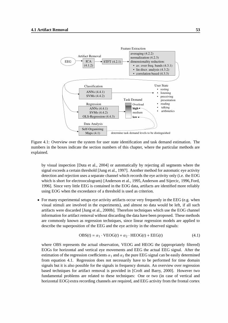
4.1 Artifact Removal 53
Figure 4.1: Overview over the system for user state identification and task demand estimation. Thenumbers in the boxes indicate the section numbers of this chapter, where the particular methods areexplained.
by visual inspection [Duta et al., 2004] or automatically by rejecting all segments where thesignal exceeds a certain threshold [Jung et al., 1997]. Another method for automatic eye activitydetection and rejection uses a separate channel which records the eye activity only (i.e. the EOGwhich is short for electrooculogram) [Anderson et al., 1995,Anderson and Sijercic, 1996,Ford,1996]. Since very little EEG is contained in the EOG data, artifacts are identified more reliablyusing EOG when the exceedance of a threshold is used as criterion.
• For many experimental setups eye activity artifacts occur very frequently in the EEG (e.g. whenvisual stimuli are involved in the experiments), and almost no data would be left, if all suchartifacts were discarded [Jung et al., 2000b]. Therefore techniques which use the EOG channelinformation for artifact removal without discarding the data have been proposed. These methodsare commonly known as regression techniques, since linear regression models are applied todescribe the superposition of the EEG and the eye activity in the observed signals:
OBS(t) = α1 · VEOG(t) + α2 · HEOG(t) + EEG(t) (4.1)
where OBS represents the actual observation, VEOG and HEOG the (appropriately filtered)EOGs for horizontal and vertical eye movements and EEG the actual EEG signal. After theestimation of the regression coefficients α1 and α2 the pure EEG signal can be easily determinedfrom equation 4.1. Regression does not necessarily have to be performed for time domainsignals but it is also possible for the signals in frequency domain. An overview over regressionbased techniques for artifact removal is provided in [Croft and Barry, 2000]. However twofundamental problems are related to these techniques: One or two (in case of vertical andhorizontal EOG) extra recording channels are required, and EEG activity from the frontal cortex

4.1 Artifact Removal 54
which is still slightly present in the EOG channels is mapped to all other channels by the artifactremoval procedure.
• [Berka et al., 2004] do not need extra electrode channels for artifact removal. They use thepositive half of a 40 µV 1.33Hz sine wave as artifact model and apply cross-correlation with theEEG signals to detect artifacts, which are characterized by maxima in the correlation function.Then artifactual data is replaced by the 4Hz high pass filtered signal of the artifactual datasegment. The two main problems of this approach are that high pass filtering might eliminateimportant EEG information and that the shape of the artifact model has to be determined usingprior knowledge.
• Finally, component based methods are an interesting group of artifact removal techniques whichalso do not require an extra EOG channel. Principal Component Analysis (PCA) or Indepen-dent Component Analysis (ICA) can be used to decompose the EEG signals in uncorrelatedcomponents (in case of PCA) or statistically independent components (in case of ICA). Theunderlying hypothesis here is that artifactual signals and signals related to neural processes areuncorrelated or emerge from independent processes so that they can be separated using methodslike PCA or ICA.
An artifact removal method which can be used in the system developed for this work should notrequire extra EOG electrodes since this would decrease the user comfort. Furthermore the use of priorknowledge to determine the shape of artifacts is problematic, since it may differ across subjects and itmay depend on the exact electrode positions. Therefore we decided to use a component based artifactremoval method in this work, namely ICA, which has been shown to be superior to PCA [Jung et al.,1998]. Component based methods have the further advantage that other (artifactual) processes thaneye activity can be detected and eliminated as well, if this is required.
The principle of ICA and its use for artifact removal is summarized briefly in the following section.A more detailed introduction on ICA can be found in [Hyvarinen and Oja, 2000].
4.1.2 Independent Component Analysis
Due to volume conduction in the body and external sources of noise (e.g. from AC lines), the signalmeasured at one electrode does not only reflect the local neural activity underneath this electrode, butit represents a superposition of several signals originating from neural and artifactual processes such asmuscular activity or noise from external electrical devices. Assuming a weighted linear superpositionof these processes, this can be expressed as follows:
x j(t) =e∑
i=1
a ji · si(t) (4.2)
Here x j(t) is the observed signal over time at electrode j, si(t) the signal corresponding to the ith
underlying process and a ji the weight which determines how much si(t) contributes to x j(t). Weassume that the number of electrode channels e is equal to the number of underlying processes orindependent components (ICs) here. This is an important assumption for ICA, which allows that theICs can be recovered from the given signals.
In practice this assumption is only approximately true. On the one hand it is possible that thenumber of independent processes is larger than the number of electrodes, when the neural processesunder each electrode are different and the signal contains additionally biological and technical arti-facts. On the other hand it may happen that in cortex regions underneath many electrodes the same

4.1 Artifact Removal 55
process takes place, namely synchronized α-activity, so that the number of independent processes issmaller than the number of electrodes. Nevertheless the approximate equality of both quantities seemssufficient for the estimation of the ICs [Makeig et al., 1996].
In matrix vector notation equation 4.2 can be reformulated as
x(t) = A · s(t) (4.3)
where x(t) is a vector containing the observed signals, s(t) a vector containing the signals correspond-ing to the ICs and A the ”mixing matrix” which defines how much each IC from s(t) contributes to thesignals x(t) observed at the different electrodes.
For detection and isolation of artifacts we are interested in the ICs which can be obtained usingthe unmixing matrix W = A−1:
s(t) = W · x(t) (4.4)
Those ICs containing artifactual data (eye activity but also AC noise and high frequent muscularactivity are well detected using ICA [Jung et al., 1998]) can be identified by visual inspection or byheuristic criteria from the training data. Using the matrix W which is estimated on the training data,the ICs can also be obtained for the validation data and for the test data. Thus it is also possibleto use cross validation to find one or more components to be rejected, so that the overall systemperformance improves most. Finally, the components which have been previously selected for removalare eliminated in the test data.
Let s′(t) be the vector where the artifact contaminated components are removed and A′ the mix-ing matrix where the columns with the indices of the artifact contaminated components of s(t) areremoved. Then an estimate for the artifact free data x′(t) is obtained by:
x′(t) = A′ · s′(t) (4.5)
The above described artifact removal process is illustrated graphically in figure 4.2.The remaining problem is the estimation of the matrices W or A. Usually only W is estimated and
A is computed as the (pseudo) inverse of W . There are several methods to obtain an estimate for W:
• Let us assume that the number of electrode channels e equals exactly the number of underly-ing (statistically independent) processes contributing to the EEG. Then the components in s(t)are independent from each other, iff only one process contributes to each component s i(t). Atthat point the central limit theorem can be used which states that the more processes are su-perimposed in one random variable, the more its probability density function (pdf) resembles agaussian pdf. Therefore our goal must be to estimate the signals si(t) for i = 1, . . . , e in a waythat their pdfs are as little gaussian as possible1 . Our actual goal is however the estimation ofthe unmixing matrix W . Therefore we use the identity si(t) = wi
T ·x(t), where wiT is the ith line
of W , so that our new goal becomes the gaussianity minimization of the pdfs of w iT · x(t) for
i = 1, . . . , e.
The gaussianity of a random variable can be measured using kurtosis which is zero for a gaus-sian random variable and becomes more negative or positive for more sub- or supergaussianrandom variables. Thus the lines wi
T of W have to be estimated such that that |kurt(wiT · x)|
becomes maximal for i = 1, . . . , e. (We denote si = wiT · x as a random variable here whose
distribution can be estimated from the time series si(t) = wiT ·x(t).) In other words the e highest
local maxima of |kurt(wiT · x)| have to be found in order to determine all e lines of W . Note
that the processes contributing to the EEG must not have a gaussian pdf themselves in order

4.1 Artifact Removal 56
Figure 4.2: Application of ICA for artifact removal in EEG data. The eye activity related artifacts areidentified by large peaks in the original data. They are isolated to the independent component 2. Afterremoval of that component and back projection of the remaining components almost artifact free datais obtained.
to make this approach work. This assumption is however usually fulfilled for EEG signals andEEG artifacts [Hyvarinen and Oja, 2000].
• Since kurtosis is very sensitive towards outliers, negentropy can be used for estimating thegaussianity of a random variable. Let g be a gaussian random variable with Cov(w i
T · x) =Cov(g) and let H denote the operator which computes the entropy of a random variable.
WhenJ(wT
i · x) = H(g) − H(wTi · x) (4.6)
is maximal, the density of wiT · x is as little gaussian as possible, since a gaussian density
has the highest entropy among all random variables of equal variance. A drawback of thisapproach is that for the computation of the entropy (non-parametric) estimates for pdfs of w i
T ·xfor i = 1, . . . e have to be computed (histograms are not sufficient) which can be difficult inpractice [Hyvarinen and Oja, 2000]. Therefore negentropy is often estimated using kurtosis,where the outlier problem arises again.
• The minimization of mutual information is a criterion for the estimation of independent com-ponents, which is inspired by information theory. Although the principle of gaussianity mini-mization to find independent components is not used here explicitly, it can be shown, that thisapproach is equivalent to the maximization of negentropy [Hyvarinen and Oja, 2000]. There-fore it can serve as a rigid mathematical justification for the more intuitive reasoning above,
1If the number of processes is larger then the number of electrode channels, the goal remains the same: When as littleprocesses as possible are superimposed in one signal, the gaussianity of the corresponding pdf is minimized. Only in therare case when there are less processes contributing to the EEG than electrode channels this approach becomes problematic.

4.1 Artifact Removal 57
which finally leads to kurtosis maximization or negentropy minimization. The mutual informa-tion of the random variables s1, . . . se which belong to the time series s1(t), . . . se(t) is defined asfollows:
MI(s1, . . . , se) =e∑
i=1
H(si) − H(s1, . . . , se) (4.7)
It is zero, when the sum of entropies of the single random variables equals the joint entropyof all random variables. If the joint entropy is smaller than the sum of single entropies, thatmeans that one or more random variables can be used to predict partly the values of one ormore others. Random variables which can be used to predict the values of each other arenot anymore independent from each other however. Therefore minimization of the mutualinformation maximizes the independence between the random variables which belong to thecomponents to be estimated.
• The infomax algorithm [Bell and Sejnowski, 1995] attempts to maximize the following crite-rion:
L = H(g1(wT1 x), . . . , ge(wT
e x)) (4.8)
where the arguments of the joint entropy operator can be interpreted as outputs of artificialneurons with non-linear activation functions gi(·) and weight vectors wi.
If we ignore the activation functions gi(·) for a moment (or set them to the identity), we obtainthe joined entropy H(s1, . . . , sn) from equation 4.7. Maximization of the joined entropy wouldlead to minimization of the mutual information, if the sum of the single entropies was almostconstant. For signals with a kurtosis larger then three, which is usually the case for EEG signals,this has been found to be a valid assumption [Bell and Sejnowski, 1995]. If however only thelinear functions wT
i x were used as arguments of the joint entropy, it could be increased simplyby increasing the variances of the arguments, i.e. the norm of wi. This is no more possible whenwT
i x is passed to a non-linear squashing function such as tanh(·) and the output of the squashingfunction is used as argument for operator computing the joint entropy [Bell and Sejnowski,1995].
Other conditions for the applicability of the infomax algorithm are that the signal sources mustreally be independent, that the signals are virtually not delayed by the ”mixing medium” be-tween source and sensors (liquor, bone and skin in case of EEG signals) and that there is asufficient number of independent processes (which is at least equal to the number of sensors).All these conditions seem to be fulfilled for EEG data [Makeig et al., 1996], so that the infomaxalgorithm is now widely applied for artifact removal in EEG data (see for instance [Jung et al.,2000a, Jung et al., 2000b, Delorme and Makeig, 2004]).
In this work ICA weights (i.e. the lines of the unmixing matrix W) are estimated using the imple-mentation of the infomax algorithm from the MATLABTM Open-Source toolbox EEGLAB [Delormeand Makeig, 2004]. The actual algorithm which maximizes the criterion in equation 4.8 is basically agradient ascent on L with respect to the weights in W . Its presentation is omitted, since it would gobeyond the scope of this work. It can be found in [Bell and Sejnowski, 1995].

4.2 Feature Extraction 58
4.2 Feature Extraction
4.2.1 Obtaining Feature Vectors
The features extracted from the time signal of each electrode channel represent the signal’s frequencycontent for a short time segment. For each electrode channel two seconds long segments which overlapone second are extracted using a hanning window. Then a short time Fourier transform (STFT) iscomputed for each segment according to
STFT(r, ω) =∞∑
m=−∞x[r + m] · w[m] · e− jωm (4.9)
where r is the index of the current time segment, ω the frequency for which the STFT is computed andw[·] denotes the windowing function which is used to extract the segment from the continuous signalx[·]. (In practice the bounds of the sum in equation 4.9 must be adapted in a way, that the maximaland minimal values of x[·] and w[·] are not exceeded.)
For a given signal the result of STFT(r, ω) is complex valued and contains information aboutamplitude and phase shift for the time segment r and the frequency ω. Since the amplitude value onlyis the information we are interested in, the phase is eliminated by taking the absolute value of theSTFT result. Thus a spectrogram is obtained:
spectrogram[r, ω] = |S T FT [r, ω]|2 (4.10)
Since two seconds long time segments are considered, we end up with an amplitude value for eachfrequency band of 1
2 Hz width for each time segment and electrode channel, which we call a feature.Remember that time segments overlap one second, so that new features for the different frequencybands are obtained every second (figure 4.3).
Features from the different electrode channels are concatenated to form one large feature vector.Let E1, . . . , Ee be the set of electrodes which are used for recording and let furthermore NE be thenumber of features which are obtained per electrode. (Since we have a 1
2 Hz resolution NE equals tothe width of the considered frequency range in Hz times two.) The value corresponding to a particularfeature for an arbitrary time segment is denoted by xi. Then for this time segment and electrode Ei,we obtain the feature vector
xEi =
x1...
xNE
for i ∈ {1, . . . , e} (4.11)
The final feature vector for this time segment is obtained by concatenating the feature vectors ofall electrodes:
x =
xE1
...
xEe
=
x1...
xNE
xNE+1...
xN
(4.12)
where N = e ·NE is the total number of features. (Note that we assume to have the same number offeatures per electrode.) In a typical setting of the data collection conducted for this work (see chapter
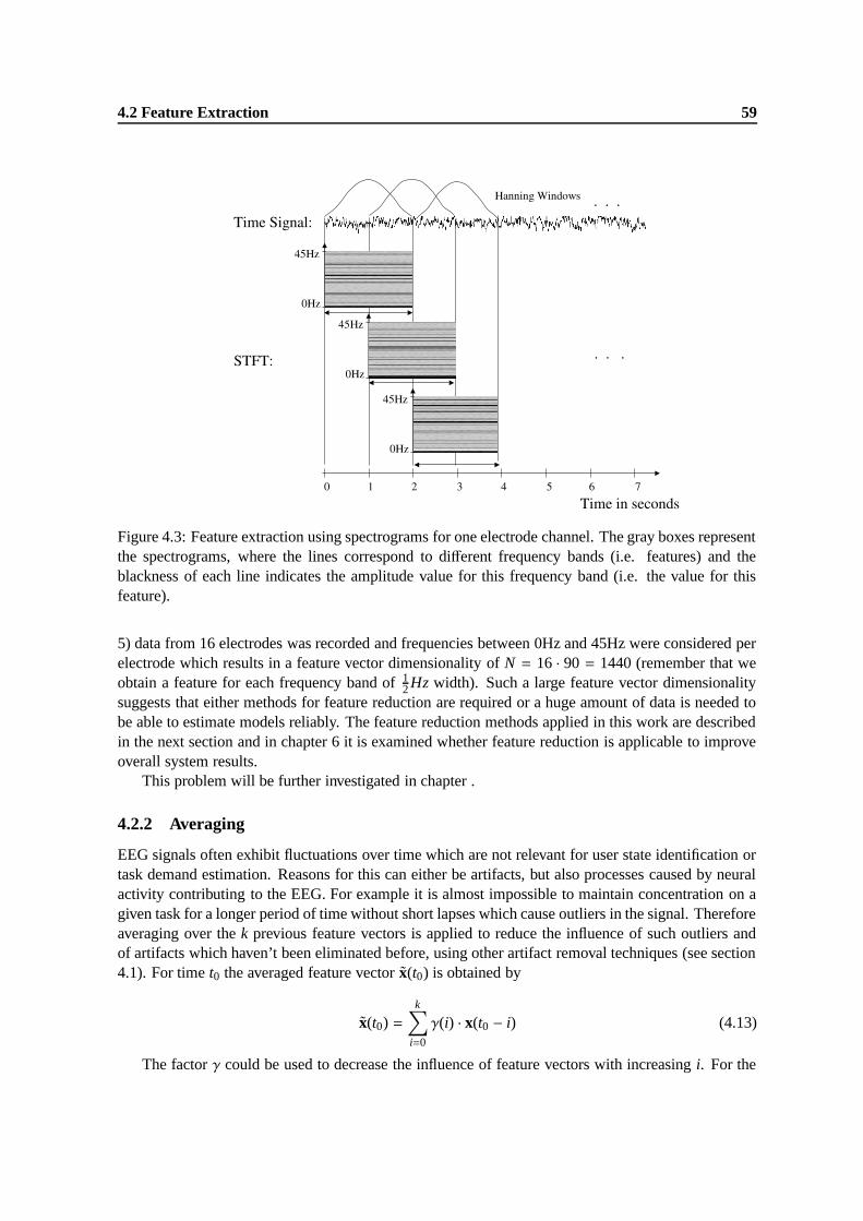
4.2 Feature Extraction 59
Figure 4.3: Feature extraction using spectrograms for one electrode channel. The gray boxes representthe spectrograms, where the lines correspond to different frequency bands (i.e. features) and theblackness of each line indicates the amplitude value for this frequency band (i.e. the value for thisfeature).
5) data from 16 electrodes was recorded and frequencies between 0Hz and 45Hz were considered perelectrode which results in a feature vector dimensionality of N = 16 · 90 = 1440 (remember that weobtain a feature for each frequency band of 1
2 Hz width). Such a large feature vector dimensionalitysuggests that either methods for feature reduction are required or a huge amount of data is needed tobe able to estimate models reliably. The feature reduction methods applied in this work are describedin the next section and in chapter 6 it is examined whether feature reduction is applicable to improveoverall system results.
This problem will be further investigated in chapter .
4.2.2 Averaging
EEG signals often exhibit fluctuations over time which are not relevant for user state identification ortask demand estimation. Reasons for this can either be artifacts, but also processes caused by neuralactivity contributing to the EEG. For example it is almost impossible to maintain concentration on agiven task for a longer period of time without short lapses which cause outliers in the signal. Thereforeaveraging over the k previous feature vectors is applied to reduce the influence of such outliers andof artifacts which haven’t been eliminated before, using other artifact removal techniques (see section4.1). For time t0 the averaged feature vector x(t0) is obtained by
x(t0) =k∑
i=0
γ(i) · x(t0 − i) (4.13)
The factor γ could be used to decrease the influence of feature vectors with increasing i. For the

4.3 Feature Reduction 60
experiments in this work it was set to one.
4.2.3 Normalization
Feature values for different frequency bands might have different ranges and different offsets. How-ever a large range of a certain feature does not necessarily imply its large importance for classifica-tion. Furthermore, the transformation of all features to a known interval is of advantage to achievequick convergence of the training procedures for some classifiers such as neural networks (see section4.5.1.5). Therefore, three simple normalization techniques are investigated:
GlobalNorm: On the training data mean and variance is calculated for each electrode and each fre-quency band. The obtained values are then used for mean subtraction and variance normaliza-tion on the training, validation and test data:
Let xi be the mean for the ith feature over the whole training set and σ2i the estimate for the
variance of this feature. For a given feature value xi of an arbitrary data set the normalizedfeature value xnorm
i is then obtained by
xnormi =
xi − xi
σi(4.14)
UserNorm: Mean and variance normalization for each frequency band is performed separately ontraining, validation and test data. If one of these data sets contains data from more than onesubject, mean and variance is also computed separately for each subject. Then the same nor-malization procedure as in equation 4.14 is applied to obtain the normalized feature values.
RelPower: To preserve relations of feature values across frequency bands, the feature value for eachfrequency band is divided by the sum of feature values over all frequency bands, which assuresthat each feature value falls within [0,1]. For a given feature vector x of dimension N thenormalized value xnorm
i for the ith feature xi is computed by
xnormi =
xi∑N
j=1 xi(4.15)
Note that a possible drawback of this method is, that information about the relation of the(total) power between adjacent feature vectors gets lost, since the sum all components of thenormalized feature vector equals to 1.
4.3 Feature Reduction
As mentioned above the dimensionality of the obtained feature vectors can be very high, when thenumber of used electrode channels and the considered frequency range per electrode channel are suf-ficiently large. Feature reduction might help here to improve the reliability of the trained models,especially in situations where training data is very sparse. Furthermore one can expect, that featurereduction methods remove those features which mainly contain noise and which are therefore detri-mental to the overall system performance. Several methods for feature reduction are investigated inthis work.

4.3 Feature Reduction 61
4.3.1 Averaging over Frequency Bands
A very straight forward method for feature reduction is to combine features by averaging over adjacentfrequency bands (i.e. adjacent features) of one feature vector. It is either possible to take always afixed number of features over which averaging is performed or to put features in physiologicallymeaningful groups, which could be for example the frequency ranges of the commonly distinguishedEEG frequency bands (see table 2.2) or of their sub-bands.
4.3.2 Linear Discriminant Analysis (LDA)
Linear discriminant analysis (LDA) is a popular method for feature reduction in classification prob-lems with a large number of features. In domains like face recognition [Li et al., 1999] or speechrecognition [Haeb-Umbach and Ney, 1992] it is commonly applied. In this work it is used to per-form feature reduction on the user state data. The underlying idea of LDA is that the feature vectordimensionality is reduced while the loss of discrimination information by eliminating features is keptminimal.
Let c1, . . . cK be the classes of a classification problem and let the feature vectors to be classifiedhave the form x = (x1, . . . xN)T . LDA attempts to find a linear function f of all features so thatdifferences between feature vectors can be expressed in a single variable, namely in the value of f :
f (x) = Y = xT · b (4.16)
where b = (b1, . . . bN )T is the vector of discriminant coefficients which weight each feature accordingto its importance for the discrimination between the given classes. Feature reduction can be performedby ranking all features according to the absolute value of their discriminant coefficient and selectingthe k highest ranked features to be included in a new feature vector. Each of these features is thenmultiplied with its discriminant coefficient and renormalized using one of the methods described insection 4.2.3. (Renormalization is required for some classification methods as mentioned above.)
The remaining problem is to find the discriminant vector b which must have the property that ismaximizes the ratio of the between class variance and the within class variance after all feature vectorshave been projected in the one dimensional ”discriminant space” using equation 4.16. Formally thevalue of γ in the following expression has to be maximized:
γ =
∑Ki=1 Rci(Yci − Y)2
∑Ki=1∑
x∈ci( f (x) − Yci)2
(4.17)
Y denotes the mean over the discriminant values of all feature vectors. The centroid Yci for class ci
which is computed according to
Yci =1
Rci
∑
x∈ci
f (x) (4.18)
where Rci denotes the number of training examples for class ci.By substituting equation 4.16 into equation 4.17 we obtain the final criterion to be maximized
which explicitly depends on b:
γ =bT BbbT Wb
(4.19)

4.3 Feature Reduction 62
The between class scatter matrix B and the within class scatter matrix W of equation 4.19 aredefined as follows:
B =K∑
i=1
(xci − x)T · (xci − x) (4.20)
W =K∑
i=1
∑
x∈ci
(x − xci)T · (x − xci ) (4.21)
where xci denotes the mean over all feature vectors of class ci and x denotes the mean over all featurevectors.
The criterion 4.19 can be maximized by setting its derivative with respect to b to zero:
∂γ
∂b!= 0
This results in the following eigenvalue problem:
(B − γW)b = 0 (4.22)
The eigenvector b for the largest eigenvalue γ corresponds to the desired discriminant vector sinceit maximizes the criterion 4.19. Note that if the feature vector dimensionality is very high and trainingdata is sparse, the matrices W and B are likely to be almost singular which can be easily seen fromtheir definitions in equations 4.20 and 4.21. In this case LDA is not applicable for feature reduction,since the eigenvalue problem in equation 4.22 does not have a stable solution. In [Li et al., 1999]the application of the QZ-algorithm for the numerical solution of the eigenvalue problem is proposedwhich succeeds to find a stable solution in cases where other algorithms (e.g. simple matrix inversion)fail. The QZ-algorithm is applied in the LDA algorithm which has been implemented for this work.Nevertheless we will see in section 6.1.7 that in some cases too little data is available, so that LDAcan not be applied.
4.3.3 Feature Reduction of Regression Tasks
LDA is a suitable feature reduction method for classification problems (e.g. for user state identifica-tion) which has been illustrated in the previous section. The problem of task demand estimation hashowever much more the properties of a regression task, since task demand is originally a continuousscaled variable. Therefore some problems would arise, if LDA-based feature reduction was appliedhere:
• For a continuous scaled dependent variable, no finite set of ”labels” (in analogy to class labels)for the different feature vectors exists.
• If the dependent variable of a regression task was ordinally scaled and if it had only a finitenumber of possible values, each value of this variable could be interpreted as a class label, sothat LDA could be applied. This is actually the case for task demand estimation, since we areconsidering only different levels of task demand: low, medium, high, overload. However LDAdoes not respect the relation between such labels, i.e. an important part of information containedin the data would not be used for LDA-based estimation of the features’ discriminative power.

4.3 Feature Reduction 63
A feature reduction method which is suitable for regression tasks is to consider the correlation co-efficient between each feature and the dependent variable. Similarly to LDA based feature reduction,features can be ranked according to the absolute value of their corresponding correlation coefficient,which is computed for the feature xi as follows:
rxi ,y =
∑Rj=1(x( j)
i − xi)(y( j) − y)∑R
j=1(x( j)i − xi)2 ·∑R
j=1(y( j) − y)2(4.23)
where x( j)i denotes the ith feature of the jth feature vector, xi the mean of the ith feature value over all
feature vectors, y( j) the value of the dependent variable belonging to the jth feature vector and y themean over all values of the dependent variable.
When using this method the occurrence of multi-collinearities is very likely, especially when thenumber of features is high. In other words, it is very likely that features are selected which are stronglycorrelated with each other. This problem could be overcome by the computation of the uncorrelatedprojections of the features using principal component analysis (PCA) prior to feature reduction. Thenthose components could be selected as features which are best correlated with the dependent variablewithout having the problem of multi-collinearities. PCA has however the same limitations as LDA,since an eigenvalue problem has to be solved to obtain the principal components which does not havea stable solution in case of high feature vector dimensionality and data sparseness.
Finally methods like forward selection or backward elimination which describe the data using alinear regression model could be used for feature reduction [Chatterjee and Price, 1991]. With sucha linear regression model one tries to find a minimal subset of features which predict the dependentvariable best.
• Forward selection starts with a regression function which includes only that feature which iscorrelated best with the dependent variable. This regression function is then extended by succes-sively adding that feature which is best correlated with the residuals obtained from the previousregression function estimation. This procedure is continued until a certain number of featureshas been included or until the sum of the squared residuals falls below a predefined threshold.Thus features which explain the dependent variable are selected in a more sophisticated waythan in case of the correlation based method proposed above. However forward selection ismuch more time consuming, since in each step one regression function has to be derived andthe correlation between the residuals and all the remaining features has to be computed. Finallyforward selection does not guarantee that multi-collinearities are avoided, but it makes only surethat in each step that feature is selected which minimizes the sum of the squared residuals in thenew regression function more than any other feature. Note that this is not necessarily the casefor the correlation based method.
• The starting point for backward elimination is the linear regression function which includesall features. Now those features are eliminated successively which reduce least the sum ofthe squared residuals. It can be shown that the feature to be eliminated next must have thelowest t-value (for the test statistic that the corresponding regression coefficient is zero) of allcandidates [Chatterjee and Price, 1991]. Backward elimination is better suited to cope withthe problem of multi-collinearities, since those features with a low t-value either don’t explainthe dependent variable well or they are highly correlated with other features which are alreadyincluded in the regression function. This elimination procedure can be continued until thelowest t-value is above a certain threshold. Similar to forward selection, the computational effort

4.4 Self-organizing Maps (SOMs) for Data Analysis 64
required for this feature reduction method is much higher compared to the correlation basedapproach, since in each step a complete regression function must be estimated. Furthermore itsapplication becomes impossible for too large feature vectors and sparse training data since thenthe matrix inversions required for the regression estimation can not be computed anymore (seealso section 4.5.3).
Due to the problems of forward and backward selection concerning computational resources andhigh feature vector dimensionalities, only the correlation-based method which has been describedabove is used in this work. For the same reasons no PCA to uncorrelate features with each otheris performed before computing correlations between features and the dependent variable. Resultsobtained using this feature reduction methods are reported in section 6.2.7.
4.3.4 Problems of Feature Reduction Methods
One common drawback of almost all feature reduction methods described above (LDA for classifi-cation tasks and correlation or linear regression based methods for regression tasks) is that they arelinear models. In case of LDA linear separability between the classes is assumed, the methods forfeature reduction in regression tasks assume a linear relationship between the features and the depen-dent variable. Furthermore LDA, PCA-based decorrelation techniques and backward selection are notapplicable in situations of data sparseness paired with high feature dimensionality.
Therefore, other methods for feature reduction have to be investigated in the future which over-come these limitations. For classification problems a promising approach which can deal with highfeature dimensionality in cases of sparse training data has been proposed for example in [Mitchellet al., 2004]. Nevertheless the application of the methods proposed above yields acceptable results aswell (see section 6).
4.4 Self-organizing Maps (SOMs) for Data Analysis
4.4.1 Motivation
Self-organizing maps (SOMs) represent a sophisticated technique for clustering data which has beenoriginally proposed by Tevu Kohonen [Kohonen, 1995]. Compared to traditional clustering tech-niques such as k-means, the main advantage of SOMs is that proximity relations between clusterscan be better visualized: While in traditional methods proximity is given by some distance measurebetween cluster prototypes, SOMs represent the proximity between cluster prototypes in a two orthree dimensional grid. Consider the example in figure 4.4. From the euclidean distances betweenthe clusters (determined by the k-means algorithm for example) it is not straight forward and in anycase difficult to infer the proximity relation which is found by a SOM. While this is also not requiredwhen results from cluster analysis are simply passed to the next step of computational processing, aproximity relation which can be visualized is extremely helpful for manual data analysis. Note thatfor many applications (and also in this work) not the real distances between prototypes in featurespace are displayed on the grid. Instead the relation holds, that points which are close together onthe grid correspond to prototypes which are close together in feature space. For many data analysisapplications this is sufficient or even desirable.
In this work SOM-based clustering is used to gain insight into the structure of the task demanddata. Features are extracted as described in the previous sections and then SOMs are trained withfeature vectors from different task demand levels. For each feature vector the best matching unit

4.4 Self-organizing Maps (SOMs) for Data Analysis 65
Figure 4.4: Comparison of the output of a traditional clustering algorithm (e.g. k-means) and of aSOM. While the traditional method outputs only distances between clusters, SOMs can be used tovisualize the proximity relations between clusters on a grid.
(BMU) on the grid is computed and visualized which allows easy analysis of the spatial relationsbetween feature vectors corresponding to different task demand levels. The BMU for a given featurevector is the unit on the grid to which the prototype with the smallest distance (in feature space) tothat feature vector belongs (see also figure 4.7).
Feature vectors with a large (euclidean) distance in feature space have BMUs which are also faraway from each other on the grid, while for vectors with smaller distances the corresponding BMUsare also closer together or they are even identical. Therefore the spatial relations between BMUswhich belong to feature vectors for different task demand levels can be used to make inferences abouthow well these task demand levels can be discriminated.
Figure 4.5 shows two SOMs together with their BMUs, one trained on data from all four taskdemand levels, the other one trained on data from low and high task demand only. When all four taskdemand levels are considered, it can be seen that the BMUs belonging to feature vectors for mediumtask demand overlap a lot with those belonging to feature vectors for low and high task demand. Thisindicates that medium task demand can not be distinguished well from the other two task demandlevels by some prediction method (i.e. a classifier or a regression method). In the other SOM one findsthat BMUs belonging to feature vectors for low and high task demand are well separated suggestingthat a prediction method can discriminate well between these two task demand levels. In section 6.2.1the SOMs trained on task demand data from other recording sessions are shown and inferences whichcan be made from their analysis are discussed. Note however that one can not necessarily infer theperformance of a prediction method only from the analysis of SOMs. It can only provide valuablehints which have to be verified experimentally using the prediction method in question. A goodexample for this are feature vectors for task demand level overload which are well separated from thefeature vectors for other task demand levels in the SOM in figure 4.5, but which are strongly confusedwith these feature vectors by all prediction methods examined in this work. (For more details aboutthat problem, please refer to section 6.2.1.)
4.4.2 Principle
Two different spaces must be distinguished for SOMs (figure 4.6):
• The map: This low dimensional (mostly two dimensional) space contains several units calledneurons which are organized in a regular grid. Neurons are connected to adjacent neurons by
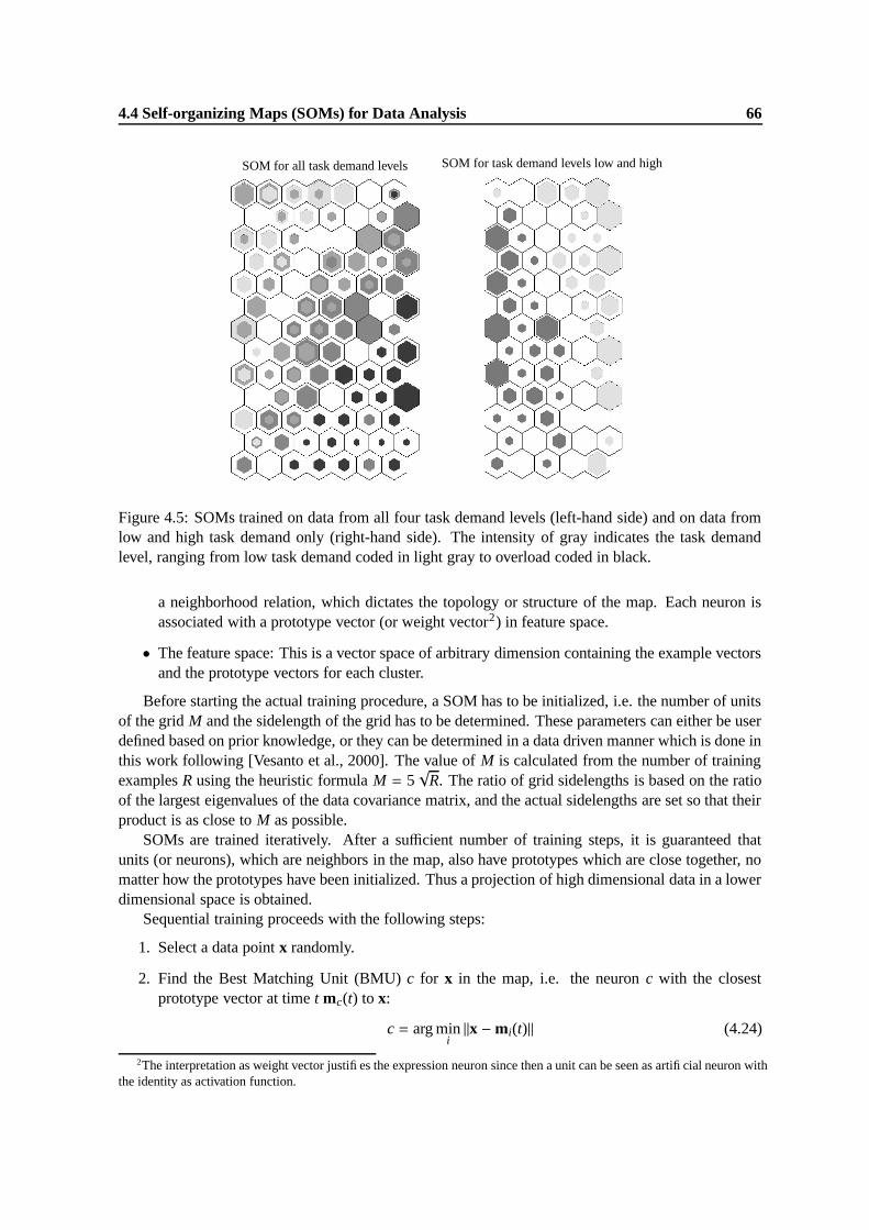
4.4 Self-organizing Maps (SOMs) for Data Analysis 66
SOM for all task demand levels SOM for task demand levels low and high
Figure 4.5: SOMs trained on data from all four task demand levels (left-hand side) and on data fromlow and high task demand only (right-hand side). The intensity of gray indicates the task demandlevel, ranging from low task demand coded in light gray to overload coded in black.
a neighborhood relation, which dictates the topology or structure of the map. Each neuron isassociated with a prototype vector (or weight vector2) in feature space.
• The feature space: This is a vector space of arbitrary dimension containing the example vectorsand the prototype vectors for each cluster.
Before starting the actual training procedure, a SOM has to be initialized, i.e. the number of unitsof the grid M and the sidelength of the grid has to be determined. These parameters can either be userdefined based on prior knowledge, or they can be determined in a data driven manner which is done inthis work following [Vesanto et al., 2000]. The value of M is calculated from the number of trainingexamples R using the heuristic formula M = 5
√R. The ratio of grid sidelengths is based on the ratio
of the largest eigenvalues of the data covariance matrix, and the actual sidelengths are set so that theirproduct is as close to M as possible.
SOMs are trained iteratively. After a sufficient number of training steps, it is guaranteed thatunits (or neurons), which are neighbors in the map, also have prototypes which are close together, nomatter how the prototypes have been initialized. Thus a projection of high dimensional data in a lowerdimensional space is obtained.
Sequential training proceeds with the following steps:
1. Select a data point x randomly.
2. Find the Best Matching Unit (BMU) c for x in the map, i.e. the neuron c with the closestprototype vector at time t mc(t) to x:
c = arg mini||x −mi(t)|| (4.24)
2The interpretation as weight vector justifies the expression neuron since then a unit can be seen as artificial neuron withthe identity as activation function.

4.4 Self-organizing Maps (SOMs) for Data Analysis 67
Figure 4.6: Map and feature space of a SOM, both of dimensionality two. For each unit on the gridthe corresponding prototype is shown. In the state depicted here, the SOM is already trained, i.e.units which are close together in the map correspond to prototype vectors which are close together infeature space.
where i is an index over all neurons in the map.
3. Now the prototype vector of each unit is altered according to the following update rule:
mi(t + 1) = mi(t) + α(t)hci(t)[x −mi(t)] (4.25)
Here α(t) is the learning rate, and hci(t) is the neighborhood kernel around the BMU c. Theneighborhood kernel usually decreases with increasing distance between c and the unit i towhich the vector mi(t) belongs. Furthermore it is non-increasing with respect to the time t. Agauss kernel
hci(t) = ed(c,i)2
σ2t
with an arbitrary distance function d(·, ·) on the grid (e.g. a block distance) and a value of σ t
which depends somehow on t would be suitable for example.
Different stopping criteria are applicable for this algorithm. One common choice is to abort it,when the update quantities for the prototype vectors drop below a threshold.
Equation 4.25 can be interpreted as follows: All prototypes mi are moved in the direction of theexample x. Prototypes are altered more, the larger the distance between m i and x, and the smaller thedistance between the BMU c and the unit i corresponding to the prototype m i. Thus even prototypeswhich are far away from x are altered little, when their corresponding neuron in the map is far awayfrom the BMU c, while other prototypes which are far away as well from x are altered a lot, whentheir corresponding unit is close to the BMU c or when it is c itself (see figure 4.7).
Training is often divided in two phases. First a large neighborhood radius is chosen (i.e. h de-creases slowly with increasing distance from the BMU) and the learning rate is large as well, so that allprototypes migrate quickly close to their final positions. In the second phase fine tuning is performedwith a small neighborhood radius and a small learning rate.
SOMs can also be trained in a batch manner where all data points are considered at one time. Thatmeans that all data points play a role for the update of an arbitrary prototype m i which belongs to unit

4.5 Classification and Regression 68
Figure 4.7: Update of prototypes during SOM training. While a prototype corresponding to a neuronwhich is far away from the BMU is altered little (mi), another prototype which has a neuron close tothe BMU is altered much more (m j).
i:
mi(t + 1) = α(t)
∑Rj=1 hc j i(t)xi(t)∑R
j=1 hc j i(t)(4.26)
where j = 1, . . .R is the index over all training examples and c j = arg maxk ||x j −mk(t)||, i.e. c j isthe BMU for the training example x j.
Similarly to the sequential training algorithm one can see here that the new prototype vectormi(t + 1) is influenced most by those data points x j for which the BMU c j is close to the neuron i onthe map. For this work the SOM implementation of the MATLABTM SOM Toolbox [Vesanto et al.,2000] was used, where batch training is performed in two phases (approximate learning and finetuning phase) as explained above. Note that batch training and sequential training generally convergeto the same results, so that the explanations given above for the sequential training algorithm are validfor the batch training algorithm as well.
4.5 Classification and Regression
To determine the user state for a given feature vector, classification techniques must be applied whichcompute a mapping
fc : X→ C (4.27)
where X denotes the feature space and C = {c1, . . . cK} the set of possible class labels.In contrast to that, task demand is measured on a continuous or at least on an ordinal scale.
Therefore regression functions are suitable to estimate the task demand level for given a feature vector.A regression function computes a mapping:
fr : X→ R (4.28)
Note that if the dependent variable in a regression task can only have a finite number of values(which is for example the case when this variable is ordinally scaled), also classification techniques

4.5 Classification and Regression 69
can be applied. Then the feature vectors which belong to a particular value of the dependent variableare put into one class, whose class label is that particular value. In this case however the informationabout the relation between values of the dependent variable gets lost, since class labels are usuallyunrelated to each other. The task demand levels considered in this work are ordinally scaled, so thatboth classification and regression techniques are investigated for task demand assessment (see section6.2). Remember that for exactly the same reasons LDA is applicable to the problem of task demandestimation, but the correlation-based method is expected to perform better, since it respects the ordinalscaling of the considered task demand levels (see section 4.3.3).
Two statistical machine learning methods are applied for classification and regression in this work:Artificial Neural Networks (ANNs) and Support Vector Machines (SVMs). Both concepts are ex-plained in the remainder of this section.
4.5.1 Artificial Neural Networks (ANNs)
4.5.1.1 Basic Principle
The structure of a single artificial neuron is depicted in figure 4.8. It receives several inputs x (in)1 , . . . x
(in)I ,
weights each input x(in)i with a weight wi, computes the sum of the weighted inputs and finally passes
the weighted sum to an ”activation” function g. (The term ”activation” function is used because ofan analogy to biological neurons which generate an axonal response only if the sum of the incom-ing impulses is large enough: if the weighted sum is above a threshold (often zero) the value of theactivation function is positive (or close to one), otherwise it is be negative (or positive but close tozero).) Common activation functions are ”squashing functions” which map an arbitrary input to acertain interval (e.g. g(h) = tanh(h) or g(h) = 1
1+ex ), linear functions or gaussians. (For the latter twothe analogy to biological neurons does not hold.) Mathematically the relation between neuron inputand output can be formulated as follows: Let x(in) = (x(in)
1 , . . . , x(in)I )T be a vector of neuron inputs, and
w = (w1, . . . ,wI)T the weight vector of the neuron. Then the neuron computes the output function
x(out)(x(in)) = g([x(in)]T w) (4.29)
Often a bias b (which plays the role of the threshold mentioned above) is subtracted from thesum of the weighted inputs before the non-linear activation function is evaluated. Then equation 4.29becomes
x(out)(x(in)) = g([x(in)]T w − b) (4.30)
When setting however x(in) = (x(in)1 , . . . , x
(in)I ,−1)T and w = (w1, . . .wI , b)T the formulation of
equation 4.29 can be used, where the bias is included implicitly when x(in) is replaced by x(in) and wby w. For simplicity we assume in the following the implicit inclusion of the bias, however we omitthe tilde.
The analogy between artificial and biological neurons which are described in section 2.1.2 doesnot only refer to the activation function but some more similarities can be found as well. The inputs ofthe artificial neurons correspond to the electrical impulses biological neurons receive via the dendrites.The weight for each input could be interpreted as the distance of the dendrite to the soma since thisdetermines the contribution of dendritic impulses to the overall potential in the soma. Finally thesubtraction of a bias and the computation of a (non-linear) activation function correspond to the wayimpulses are processed in the soma to produce an output impulse which is transmitted via the axonas explained above. The processes in biological neurons however are much more complex than thosemodeled by artificial neurons. Therefore the analogy which can be established between both conceptsis rather weak.
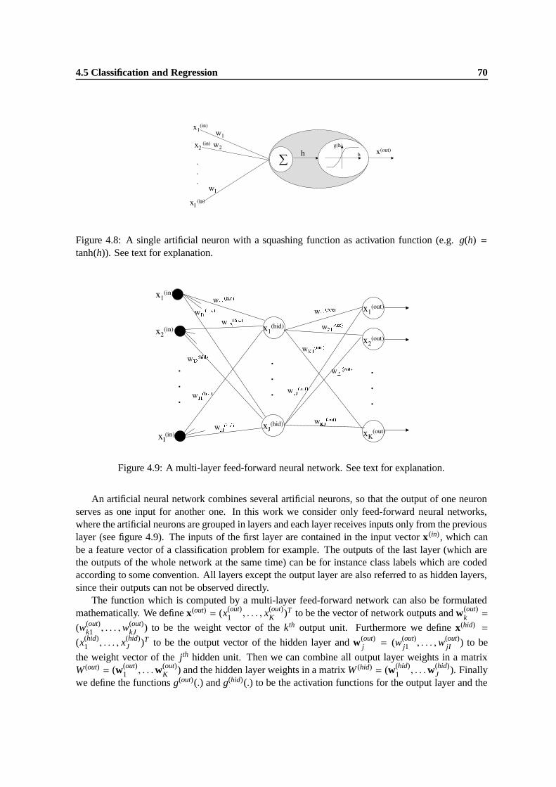
4.5 Classification and Regression 70
Figure 4.8: A single artificial neuron with a squashing function as activation function (e.g. g(h) =tanh(h)). See text for explanation.
Figure 4.9: A multi-layer feed-forward neural network. See text for explanation.
An artificial neural network combines several artificial neurons, so that the output of one neuronserves as one input for another one. In this work we consider only feed-forward neural networks,where the artificial neurons are grouped in layers and each layer receives inputs only from the previouslayer (see figure 4.9). The inputs of the first layer are contained in the input vector x(in), which canbe a feature vector of a classification problem for example. The outputs of the last layer (which arethe outputs of the whole network at the same time) can be for instance class labels which are codedaccording to some convention. All layers except the output layer are also referred to as hidden layers,since their outputs can not be observed directly.
The function which is computed by a multi-layer feed-forward network can also be formulatedmathematically. We define x(out) = (x(out)
1 , . . . , x(out)K )T to be the vector of network outputs and w(out)
k =
(w(out)k1 , . . . ,w
(out)kJ ) to be the weight vector of the kth output unit. Furthermore we define x(hid) =
(x(hid)1 , . . . , x(hid)
J )T to be the output vector of the hidden layer and w(out)j = (w(out)
j1 , . . . ,w(out)jI ) to be
the weight vector of the jth hidden unit. Then we can combine all output layer weights in a matrixW (out) = (w(out)
1 , . . .w(out)K ) and the hidden layer weights in a matrix W (hid) = (w(hid)
1 , . . .w(hid)J ). Finally
we define the functions g(out)(.) and g(hid)(.) to be the activation functions for the output layer and the

4.5 Classification and Regression 71
hidden layer respectively which take a vector of weighted sums as inputs and return an output vectorwhose components represent the outputs of the units of the corresponding layer. The network inputsare given as for the single neuron by x(in) = (x(in)
1 , . . . x(in)I )T . Now we can write:
x(out)(x(in)) = g(out)[W (out) · g(hid)(Whid · x(in))︸ ︷︷ ︸
=x(hid)
] (4.31)
In the remainder of this section the application of neural networks for classification and regressiontasks is briefly described. A more detailed description can be found in [Bishop, 1995].
4.5.1.2 ANNs for Classification Problems
Let us return to the single neuron whose behavior is described by equation 4.30. Its use for clas-sification is best illustrated geometrically. The weight vector w together with the bias b define anI-dimensional hyperplane whose orientation is given by w and whose a distance from the origin is−b||w|| (figure 4.10). If we set the neuron’s activation function g(h) = tanh(h), its output is larger thenzero if an input vector is located on that side of the hyperplane where the vector w points to (whichis the case for the example vectors depicted with ”+” in the figure), and it is smaller than zero, if theinput vector is located on the opposite side (which is the case for the example vectors depicted with”-” in the figure). Finally the neuron’s output has the exact value of zero, if the input vector is locatedexactly on the hyperplane.
Now we assign each input vector a target value which is either +1 or −1. (For a binary classifi-cation problem the target values can be interpreted as class labels.) In the following we define thatthe input vectors which are depicted with ”+” have the target value +1 and they are referred to aspositive examples, while the input vectors which are depicted with ”-” have the target value −1 andthey are referred to as negative examples. Thus the example vectors x(in) in figure 4.10 are all classi-fied correctly if we compute the network predictions by sgn(x(out)(x(in))). We conclude that a singleartificial neuron is able to discriminate between positive and negative examples as long as they can beseparated by a hyperplane. In other words, a single artificial neuron can be used as binary classifierfor linearly separable problems.
Naturally a training procedure is required before an artificial neuron can be actually used forclassification, since one can not expect that for a random initialization of the vector w positive andnegative examples are classified correctly. For the simple case where only a single neuron is used,there is an intuitive explanation of the training procedure. Starting with a randomly initialized normalvector, all training examples are considered and whenever a training example is misclassified (i.e. onthe wrong side of the hyperplane), the normal vector is moved a bit in the direction of that exampleif the example is positive, or in the opposite direction if the example is negative (figure 4.11). Math-ematically this can be described as a gradient descent on an error function which is described brieflybelow for the more general case of multi-layer feed-forward neural networks.
Note that if we have I-dimensional input vectors, we obtain an I+1 dimensional hyperplane whichpasses through the origin, if the encode the bias implicitly in the weight vector as explained above.When using an explicit bias, an I dimensional hyperplane is obtained which does not necessarily passthough the origin as shown in figure 4.10. Both formulations are completely equivalent. While thesecond one is more suitable for visualization (the behavior of a single neuron with two non-bias-related inputs can be easily visualized in a two dimensional coordinate system here), we use the firstone in the following because of its mathematical simplicity.
The classes of real-world classification problems can not always be linearly separated. Thus asingle neuron is not suitable to address such problems. Using however a multi-layer neural network
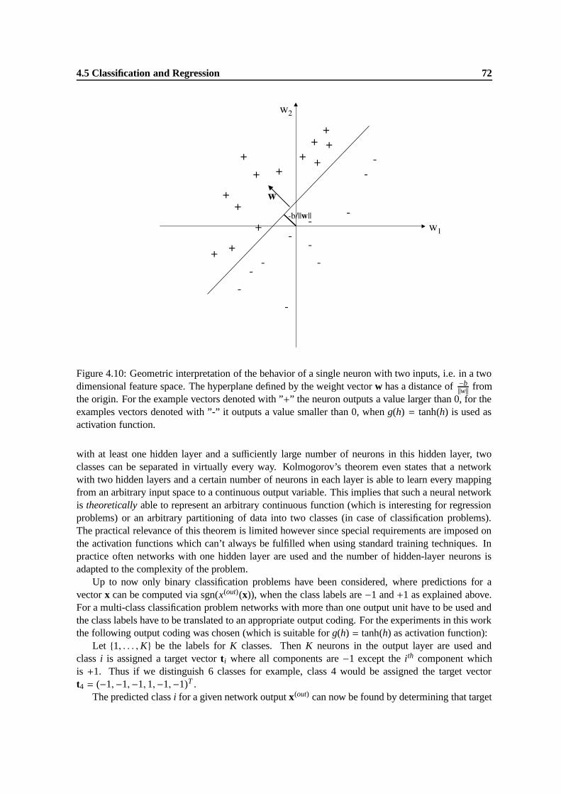
4.5 Classification and Regression 72
Figure 4.10: Geometric interpretation of the behavior of a single neuron with two inputs, i.e. in a twodimensional feature space. The hyperplane defined by the weight vector w has a distance of −b
||w|| fromthe origin. For the example vectors denoted with ”+” the neuron outputs a value larger than 0, for theexamples vectors denoted with ”-” it outputs a value smaller than 0, when g(h) = tanh(h) is used asactivation function.
with at least one hidden layer and a sufficiently large number of neurons in this hidden layer, twoclasses can be separated in virtually every way. Kolmogorov’s theorem even states that a networkwith two hidden layers and a certain number of neurons in each layer is able to learn every mappingfrom an arbitrary input space to a continuous output variable. This implies that such a neural networkis theoretically able to represent an arbitrary continuous function (which is interesting for regressionproblems) or an arbitrary partitioning of data into two classes (in case of classification problems).The practical relevance of this theorem is limited however since special requirements are imposed onthe activation functions which can’t always be fulfilled when using standard training techniques. Inpractice often networks with one hidden layer are used and the number of hidden-layer neurons isadapted to the complexity of the problem.
Up to now only binary classification problems have been considered, where predictions for avector x can be computed via sgn(x(out)(x)), when the class labels are −1 and +1 as explained above.For a multi-class classification problem networks with more than one output unit have to be used andthe class labels have to be translated to an appropriate output coding. For the experiments in this workthe following output coding was chosen (which is suitable for g(h) = tanh(h) as activation function):
Let {1, . . . ,K} be the labels for K classes. Then K neurons in the output layer are used andclass i is assigned a target vector ti where all components are −1 except the ith component whichis +1. Thus if we distinguish 6 classes for example, class 4 would be assigned the target vectort4 = (−1,−1,−1, 1,−1,−1)T .
The predicted class i for a given network output x(out) can now be found by determining that target

4.5 Classification and Regression 73
Figure 4.11: Training of a single neuron for its application as binary classifier. The example on theupper right is misclassified by the original hyperplane (dashed line). In the next training step thenormal vector of the hyperplane is moved into the direction of the misclassified example so that thenew hyperplane (solid line) does not produce this misclassification anymore.
vector for which the euclidean distance to the network output is minimal, i.e.
i = arg minj=1,...,K
||x(out) − t j||
It can easily be shown that this is equivalent to determining the index the largest component of theoutput vector x(out), i.e.
i = arg maxj=1,...,K
x(out)j
The latter method is computational more efficient, since there is no need to compare the outputvector with the target vector for each class.
4.5.1.3 ANNs for Regression Problems
For the estimation of a scalar regression function using a multi-layer feed-forward neural networkonly one output unit with a linear activation function is required (figure 4.12). If this function is setto the identity, only the weighted sum of the outputs from the hidden layer neurons is computed. Nooutput coding is required here. The output of the network can be interpreted directly as prediction ofthe dependent variable of the regression function. For the training procedure the given values of thedependent variable from the training examples can be used directly as targets. Note however that itis advisable to normalize target values before training so that they reside in a known interval (and to
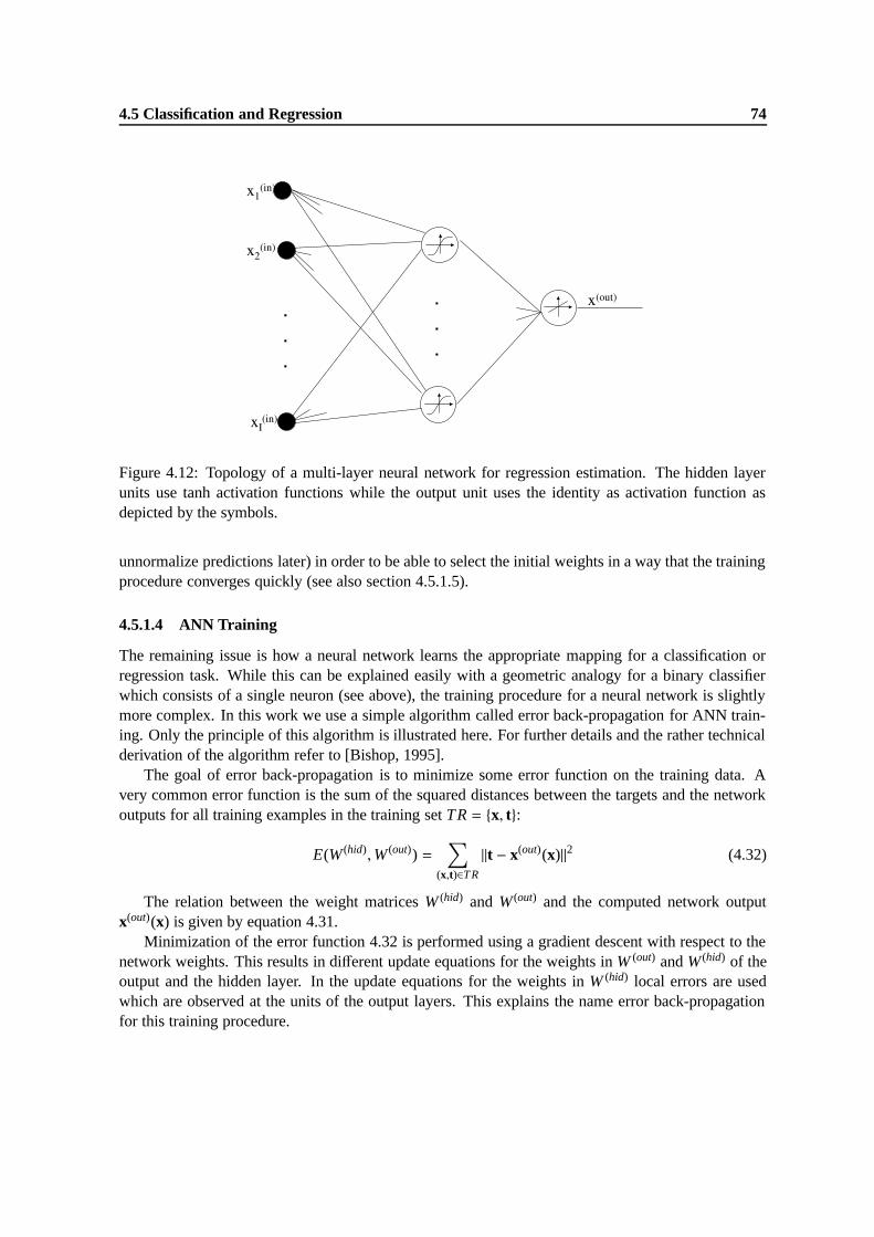
4.5 Classification and Regression 74
Figure 4.12: Topology of a multi-layer neural network for regression estimation. The hidden layerunits use tanh activation functions while the output unit uses the identity as activation function asdepicted by the symbols.
unnormalize predictions later) in order to be able to select the initial weights in a way that the trainingprocedure converges quickly (see also section 4.5.1.5).
4.5.1.4 ANN Training
The remaining issue is how a neural network learns the appropriate mapping for a classification orregression task. While this can be explained easily with a geometric analogy for a binary classifierwhich consists of a single neuron (see above), the training procedure for a neural network is slightlymore complex. In this work we use a simple algorithm called error back-propagation for ANN train-ing. Only the principle of this algorithm is illustrated here. For further details and the rather technicalderivation of the algorithm refer to [Bishop, 1995].
The goal of error back-propagation is to minimize some error function on the training data. Avery common error function is the sum of the squared distances between the targets and the networkoutputs for all training examples in the training set TR = {x, t}:
E(W (hid),W (out)) =∑
(x,t)∈TR
||t − x(out)(x)||2 (4.32)
The relation between the weight matrices W (hid) and W (out) and the computed network outputx(out)(x) is given by equation 4.31.
Minimization of the error function 4.32 is performed using a gradient descent with respect to thenetwork weights. This results in different update equations for the weights in W (out) and W (hid) of theoutput and the hidden layer. In the update equations for the weights in W (hid) local errors are usedwhich are observed at the units of the output layers. This explains the name error back-propagationfor this training procedure.

4.5 Classification and Regression 75
4.5.1.5 Practical Problems
Some practical problems must be considered for the application of neural networks in classificationor regression tasks. They are summarized briefly in this section. A more detailed discussion of theseissues is provided in [Bishop, 1995].
• When using the error function of equation 4.32 it is important to adjust the amount of trainingdata for all classes to be approximately equal, i.e. to create balanced training data. Otherwisethe network might become biased towards those classes which contain more training examples,since the minimization of the error for the examples of such classes often minimizes the overallerror function best.
• If the value of the dot product between input vectors and the weight vector h = xT w is toolarge, changes of the network weights cause virtually no change in the network output since theslope of sigmoid- and tanh- activation functions for large arguments is extremely small. Thismay lead to a very slow convergence of the training procedure. A good heuristic to avoid thisproblem is to initialize the network weights randomly to small values, e.g. from the interval[−1, 1]. The effect of small, randomly initialized weights gets lost however when the networkinputs are too large. Therefore the network inputs should be either transformed so that theirvalues reside also in a small interval around zero (again [−1, 1] is suitable for instance), or eachnetwork weight must be adapted to the range its input, so that at the end the value of h is kept ina reasonable range. In this work features are normalized before they are used as network inputsso that they have values which are at least close to [−1, 1] (see section 4.2.3). Therefore weightsare simply initialized randomly in [−1, 1] to assure reasonable fast convergence of the trainingalgorithm.
• Random weight initializations are also the reason that different local minima of the error func-tion are found, when a network is trained several times with the same training data. Whennow the process of training and evaluation of the network performance on test data is repeatedseveral times, results exhibit certain fluctuations. They can be reduced, although not avoided,when for a given training and test set more than one networks are trained and evaluated. Thenmajority decisions (in case of classification) or averaging over all network predictions (in caseof regression) can be used to obtain more stable estimates for correct class labels or regressionfunction values.
• The problem of overfitting the training data can be treated in several ways for neural net-works [Bishop, 1995]. In this work a technique commonly known as early stopping is used.The error on the validation set is computed after each training epoch, using the error functionfrom equation 4.32. The goal is to find that epoch where the validation error has its global min-imum. Using the network with the weights from this epoch, one assumes that generalizationperformance and thus the error on unseen data is best (figure 4.13). To find the global minimumof the validation error a heuristic is applied: Each time after a potential minimum (which isnot necessarily global) has been found, training is continued for a few more epochs. Only ifduring these epochs the validation error does not decrease again (or alternatively if it does notfall below the previously found minimum), training is aborted and the weights from the epochwhere the validation error was minimal are used. Otherwise training is continued. To makesure that the algorithm stops after a finite number of epochs, training is aborted as well whenthe training error drops below a certain threshold.
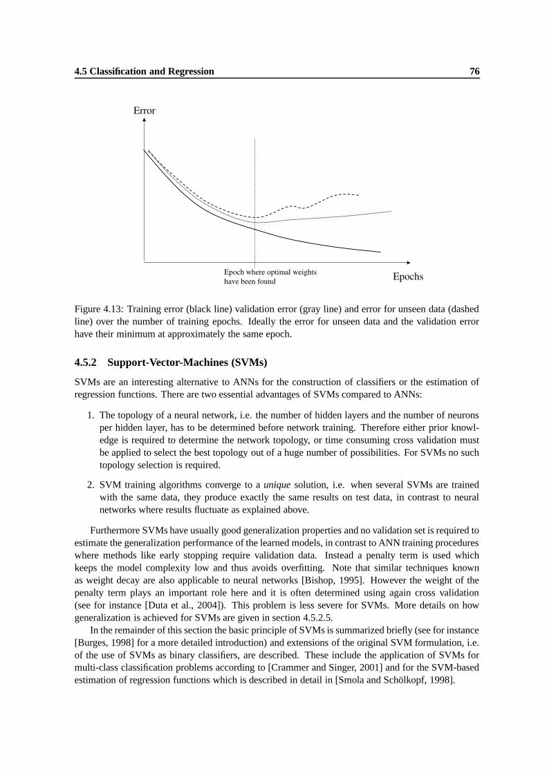
4.5 Classification and Regression 76
Figure 4.13: Training error (black line) validation error (gray line) and error for unseen data (dashedline) over the number of training epochs. Ideally the error for unseen data and the validation errorhave their minimum at approximately the same epoch.
4.5.2 Support-Vector-Machines (SVMs)
SVMs are an interesting alternative to ANNs for the construction of classifiers or the estimation ofregression functions. There are two essential advantages of SVMs compared to ANNs:
1. The topology of a neural network, i.e. the number of hidden layers and the number of neuronsper hidden layer, has to be determined before network training. Therefore either prior knowl-edge is required to determine the network topology, or time consuming cross validation mustbe applied to select the best topology out of a huge number of possibilities. For SVMs no suchtopology selection is required.
2. SVM training algorithms converge to a unique solution, i.e. when several SVMs are trainedwith the same data, they produce exactly the same results on test data, in contrast to neuralnetworks where results fluctuate as explained above.
Furthermore SVMs have usually good generalization properties and no validation set is required toestimate the generalization performance of the learned models, in contrast to ANN training procedureswhere methods like early stopping require validation data. Instead a penalty term is used whichkeeps the model complexity low and thus avoids overfitting. Note that similar techniques knownas weight decay are also applicable to neural networks [Bishop, 1995]. However the weight of thepenalty term plays an important role here and it is often determined using again cross validation(see for instance [Duta et al., 2004]). This problem is less severe for SVMs. More details on howgeneralization is achieved for SVMs are given in section 4.5.2.5.
In the remainder of this section the basic principle of SVMs is summarized briefly (see for instance[Burges, 1998] for a more detailed introduction) and extensions of the original SVM formulation, i.e.of the use of SVMs as binary classifiers, are described. These include the application of SVMs formulti-class classification problems according to [Crammer and Singer, 2001] and for the SVM-basedestimation of regression functions which is described in detail in [Smola and Scholkopf, 1998].

4.5 Classification and Regression 77
Figure 4.14: Separation between two (linearly separable) classes in a two dimensional feature spacefound by an ANN (left) and an SVM (right). While the ANN training procedure can converge toseveral possible solutions, the SVM determines a unique hyperplane which maximizes the margin κto the positive examples (denoted with ”+”) and negative examples (denoted with ”-”).
4.5.2.1 Basic principle
In their original version SVMs are binary classifiers. The most simple variant, the linear SVM, canseparate two classes in a feature space of arbitrary dimension by a hyperplane. The same problem canalso be solved by a single artificial neuron (see section 4.5.1.2). The difference between both methodscan be understood intuitively when comparing the separations which are found for linearly separableclassification problems in a two dimensional feature space by each of the classifiers (figure 4.14).
The single neuron may find different separating hyperplanes (lines in the two dimensional case),dependent on the (local) minimum of the error function to which the training procedure converges.The SVM instead determines a separation between the classes which is in a certain sense optimal. Itmaximizes the ”security margin” κ to both, the positive (denoted with ”+”) and the negative (denotedwith ”-”) training examples.
Mathematically the hyperplane which is found by an SVM is given by
wT · x + b = 0 (4.33)
where w is the normal vector of the hyperplane and b an offset which is proportional to the hyper-plane’s distance from the origin (the distance is exactly b
||w|| ). An example is classified to be positive if
wT x+ b > 0, otherwise it is classified to be negative. Let now the class label y i for a training examplexi be +1 if xi is a positive example and −1 otherwise. Then the following conditions hold for thetraining data TR = {(xi, yi)} with respect to the hyperplane defined by equation 4.33 which has beendetermined during training:
∀(xi, yi) ∈ TR : yi(w · xi + b ≥ κ) (4.34)
In other words, all training examples have a distance of at least κ from the hyperplane. (Note thatthe above conditions can only be fulfilled, if the training data is linearly separable.)
To obtain maximal margins, the value of κ has to be maximized. Division by κ and setting w = wκ
and b = bκ
results in the following condition which must be fulfilled for the training data:
∀(xi, yi) ∈ TR : yi(w · xi + b) ≥ 1 (4.35)
Now the value of κ can be maximized via the minimization of ||w||. Thus we end up with thefollowing constrained optimization problem which has to be solved to find the desired separation with

4.5 Classification and Regression 78
Figure 4.15: Two outlier examples (highlighted in gray) which make a linear separation of the classesimpossible (left) and the solution of this problem using soft margins (right).
a maximal margin. (From now on we omit the tilde in equation 4.35 for better readability):
Minimize ||w||subject to
yi(w · xi + b) ≥ 1 ∀(xi, yi) ∈ TR (4.36)
Note that the final separation is determined by only a few training vectors which are referred toas support vectors. The support vectors have the property that they are located exactly on the securitymargin.
Figure 4.15 illustrates a situation where only because of two training examples no linear separationbetween the two classes is possible anymore, although both examples are likely to be outliers. To copewith that problem soft margins are introduced, which allow that training examples violate the securitymargin at a certain cost. Equation 4.35 becomes now
∀(xi, yi) ∈ TR : yi(w · xi + b) ≥ 1 − ξi (4.37)
where ξi determines how much the margin is violated.Using soft margins, the optimization problem of equation 4.36 must be extended to:
Minimize ||w|| +C∑
i ξi
subject to
yi(w · xi + b) ≥ 1 − ξi ∀(xi, yi) ∈ TR (4.38)
C is a user-specified factor here which determines the cost for the violation of the security margin.High values of C favor little violations which results in a small margin in consequence, lower valuesof C produce more margin violations thus allowing a larger margin.

4.5 Classification and Regression 79
The optimization problem 4.38 can theoretically be solved using standard techniques for con-strained optimization. However these techniques involve the computation of matrices whose sizegrows quadratically with the feature vector dimensionality. Therefore the application of standard tech-niques becomes already unfeasible for feature vectors of medium size because of speed and memoryreasons. To overcome that problem several approximations and modifications of the standard op-timization algorithms have been developed. For more details concerning the solution of the SVMoptimization problem, please refer to [Burges, 1998].
4.5.2.2 Non-linear SVMs
SVMs are also applicable to classification tasks where classes are not linearly separable. In such acase the feature vectors x which we assume now to be elements of RN are mapped into an euclideanspace with a higher (possibly infinite) dimensionality which we call H using a mapping Φ:
Φ : RN →H
Because of several findings of statistical learning theory (see [Burges, 1998]) it is a plausibleassumption that if only the dimensionality of H is high enough, the classes can again be separatedlinearly in H . Note however that in this case the security margin is maximized only for the linearseparation in H but not for the (non-linear) separation of the classes in the original feature space.Nevertheless the generalization performance of non-linear SVMs is usually still very good. The opti-mization problem from equation 4.38 looks as follows for the non-linear case:
Minimize ||w|| +C∑
i ξi
subject to
yi
(
Φ(w) · Φ(xi) + b)
≥ 1 − ξi ∀(xi, yi) ∈ TR (4.39)
The mapping Φ is never computed explicitly, since this would be computationally very expensivefor a sufficiently high dimensionality ofH and even infeasible if the dimensionality ofH was infinite.The explicit evaluation of Φ is avoided using a method commonly referred to as ”kernel trick”:
During optimization it turns out, that the vector w can be written as linear combination of sometraining vectors, the ”support vectors”, which we define to belong to a set S V . As explained above,these vectors have the property that they lie directly on the margin and thus uniquely define the sepa-ration between the classes. Thus w becomes
w =∑
i∈S V
αixi (4.40)
where αi represent truly positive weights for the support vectors x ∈ S V .Furthermore during classification, i.e. the evaluation of sgn(w ·x+b) for some training example x
and also during optimization only dot products between feature vectors are computed. Therefore wecan define
k(xi, x j) = Φ(xi)T · Φ(x j) (4.41)
to be the dot product between two feature vectors which have been mapped before toH using Φ.Substitution of equation 4.40 in equation 4.39 and application of the identity 4.41 yields in the
following optimization problem where no explicit mapping into H is required anymore:

4.5 Classification and Regression 80
Minimize ||w|| +C∑
i ξi
subject to
yi
(
k(w · xi) + b)
≥ 1 − ξi ∀(xi, yi) ∈ TR (4.42)
The function k(·, ·) is called kernel function and it can be any function which fulfills Mercer’scondition (see [Burges, 1998] for an explanation of this condition). If this is the case it can be provedthat the kernel function computes a dot product in some high dimensional euclidean space H whichneeds not necessarily to be known.
We conclude that the kernel trick for computing the dot product between feature vectors is usefulto apply SVMs for non-linearly separable problems without increasing the amount of computationalcost tremendously. Only the evaluation of the kernel function needs usually more computation thanthe evaluation of the dot product in feature space. Therefore the computational effort for non-linearSVMs increases only by a multiplicative constant compared to linear SVMs.
Popular kernel functions are
k(x, y) = (xT · y + c)d (4.43)
k(x, y) = e||x−y||/(2σ2 ) (4.44)
k(x, y) = tanh(κ(xT · y) − δ) (4.45)
where d, σ, κ and δ are free parameters which are usually determined using cross-validation. Notethat because of the need for cross-validation to tune the kernel parameters, often linear SVMs arepreferred to non-linear SVMs when it is not known a priori that the data follows a highly non-linearrelationship.
4.5.2.3 Multiclass SVMs
Up to this point only binary classification problems have been considered in the context of SVMs.The problem of user state identification which is addressed in this work involves however the discrim-ination of more than two classes. One possibility to apply SVMs for multi-class classification is totrain an SVM for each class which discriminates the examples of this class from all others. Then thedistance from the margin computed by the different SVMs can be used as a criterion to make a finaldecision for the predicted class, if more than one SVMs decide that an example belongs to ”their”class. In this work a more elegant solution of that issue, proposed in [Crammer and Singer, 2001], isused which addresses the multi-class classification problem for SVMs directly. The function fc whichmaps a feature vector to a class label is defined here as follows:
fc(x; M) = arg maxr{Mr · x} (4.46)
fc simply decides that an example x belongs to that class r for which the similarity between x andthe prototype vector Mr for class r (expressed via the dot product of both vectors) is maximal. Thematrix M contains the prototype vectors Mr as lines.
The empirical error of the classifier in equation 4.46 on the training set TR = {(x i, yi)} can thus beformulated as:

4.5 Classification and Regression 81
Eemp =1|TR|
∑
(xi,yi)∈TR
(1 − δ fc(xi;M),yi ) (4.47)
The concept of margin maximization is introduced now by replacing (1 − δ fc(xi;M),yi ) in equation4.47 by
maxr{Mr · xi + 1 − δr,yi } −Myi · xi (4.48)
Thus the error for an example (xi, yi) is zero only if the similarity between xi and the prototypeof its correct class Myi is at least larger by one than the similarity between xi and the second similarprototype. Otherwise the error the error increases continuously.
The optimization problem to be solved for multi-class SVMs is similar to the problem for binarySVMs:
Minimize ||M||2
subject to
Myi · xi + δyi,r −Mr · xi ≥ 1 ∀r ∀(xi, yi) ∈ TR (4.49)
The incorporation of slack variables and kernels is analogous to the procedure for binary SVMswhich has been explained in sections 4.5.2.1 and 4.5.2.2. For more details please refer to [Crammerand Singer, 2001]. In this work an extension of the publicly available S V M light software [Joachims,1999] is used for SVM based multi-class classification, which embeds the above formulation in amore general framework (see [Tsochantaridis et al., 2004] for details).
4.5.2.4 Regression SVMs
For the estimation of regression functions the training examples (xi, yi) ∈ TR contain a feature vectorxi as in case of classification and a continuous value yi which is the target value of the regressionfunction f to be predicted.
The simplest case is to learn only a linear function:
f (x) = w · x + b (4.50)
Usually it is unfeasible in the presence of noise to fit data exactly to a linear function (even ifthe data follows a linear relationship). For ordinary least square regression this problem is addressedby minimizing the squared error between the values of the estimated function and the targets of thetraining examples. In case of SVM-based regression, noise is considered simply by requiring thetraining examples to lie within an ε-tube around the estimated function in order to cause no cost (seealso figure 4.16). Thus the following constraints are imposed for the estimation of f with respect tothe training data:
∀(xi, yi) ∈ TR
yi − w · xi − b ≤ εand
w · xi + b − yi ≤ ε (4.51)

4.5 Classification and Regression 82
Figure 4.16: Use of soft margins for SVM regression. The ε-tube where targets of the training datamay lie without causing a cost is shaded in gray. Only outliers which do not lie within the ε-tubecause a cost which is proportional to ξ or ξ∗ respectively.
Additionally one requires that the flattest possible function is chosen out of all functions whichfulfill the above constraints. In analogy to classification SVMs, flatness is defined here in terms of||w||, i.e. ||w|| is to be minimized to obtain the flattest function. For a more rigid justification of that,please refer to [Smola, 1998]. Intuitively the flattest function can be thought as that function whichadapts least to the noise of the training data, which is particularly evident for non-linear regressionfunctions.
Thus we have the following optimization problem for SVM regression:
Minimize ||w|| subject to
yi − w · xi − b ≤ εand
w · xi + b − yi ≤ ε ∀(xi, yi) ∈ TR (4.52)
Similarly to the classification case the introduction of soft margins makes sense here too, in orderto reduce the influence of single outliers on the estimated function (figure 4.16). Then the optimizationproblem becomes
Minimize ||w|| +C∑
i
ξi + ξ∗i
subject to (4.53)
yi − w · xi − b ≤ ε + ξiw · xi + b − yi ≤ ε + ξ∗iξi, ξ
∗i ≥ 0 ∀(xi, yi) (4.54)
Exactly in analogy to classification SVMs, kernels can be used as well to estimate non-linear

4.5 Classification and Regression 83
regression functions. Note however that here again the use of kernels requires cross-validation todetermine appropriate kernel parameters.
For the solution of the optimization problems related to SVM regression the same techniques asfor SVM classification are applied. The software S V M light [Joachims, 1999] is used in this work forSVM-based regression function estimation.
4.5.2.5 Generalization Properties of SVMs
Now that the basic concepts of SVMs are introduced their generalization properties shall be analyzedbriefly. The actual goal of each classification or regression task for which a mapping f (x) = y mustbe learned, is to minimize some error function for unknown data (i.e. the actual error Eactual). Thedata is assumed to be generated by a probability distribution P(x, y).
Eactual =
∫
c(
x, y, f (x))
dP(x, y) (4.55)
where c is an arbitrary loss function such as the squared error (y − f (x))2
Since P(x, y) is usually not known, the actual error can not be computed exactly. Neural net-works (without regularization techniques such as early stopping or weight decay, see section 4.5.1.5)approximate the actual error using the empirical error on the training set TR:
Eemp =1|TR|
∑
(x,y)∈TR
c(x, y, f (x)) (4.56)
which is clearly suboptimal since it makes overfitting very likely. Therefore in case of SVMs a penaltyterm is added to Eemp so that the following error function is minimized:
ES VM = Eemp + λ||w|| (4.57)
It has been shown above that the minimization of ||w|| corresponds to finding the hyperplane (infeature space for linear SVMs, in H for non-linear SVMs) with the maximal margin to the classesto be separated for a classification problem, or to finding the flattest function which approximatesthe data for a regression problem. The above formulation shows now that there is a relation betweenthese criteria and the approximation of the actual error in case of SVMs. The minimization of ||w|| isused here to avoid overfitting since the overall error can not be minimized simply by minimizing theempirical error only. Therefore SVMs have usually good generalization properties although no extracross-validation is required.
4.5.3 Multiple Linear Regression
Multiple linear regression is a very simple method for the estimation of regression functions. Incontrast to SVMs (with kernels) and multi-layer neural networks which can estimate non-linear func-tions, only linear relationships can be obtained using this method. Given the training data TR ={(x1, y1), . . . (xR, yR)}, the goal is to learn a function
f (x) = wT · x + b (4.58)
such that the empirical error for the training set TR is minimized. In ordinary least square (OLS)regression this is the mean square error

4.5 Classification and Regression 84
Eols =1|TR|
∑
(xi,yi)∈TR
(yi − f (xi))2 (4.59)
Now we explain how a regression function is found using OLS regression. Let the training databe
For the sake of clarity we eliminate first the parameter b from equation 4.58 by setting
w := (w(1), . . .w(N), b)T
xi := (x(1)i , . . . , x
(N)i , 1)T for i = 1, . . .R
where x( j)i denotes the jth component of the ith feature vector and w( j) the jth regression coefficient.
Then equation 4.58 becomes
f (x) = wT x
Now we define y = (y1, . . . , yR)T and
X =(
xT1
... xTR
)
Using the above definitions the regression coefficients w which minimize the error from equation4.59 are the best approximative solution of the system of linear equations:
y = X · w
Obviously an exact solution for equation 4.5.3 can only be found if the matrix X has a rank of Nwhich is usually not the case. Note that an exact solution of the equation would yield in an empiricalerror of zero, since if w = w we have
0 = ||y − X · w|| =∑
(xi,yi)∈TR
(yi − wT xi)2 = Eols
Normally the problem 4.5.3 is however either under determined or over determined. In that casean approximate solution can be computed which minimizes Eols, using the pseudo inverse X+ of X.This matrix has the important property that the estimate
w = X+ · y
for w minimizes ||y − X · w||2 which also minimizes Eols. The pseudo inverse of a matrix isusually computed using a singular value decomposition and its computation is possible even if thematrix is not square and of full rank. For a description of more properties of the pseudo inverse and anexplanation of the algorithm for singular value decomposition please refer to [Golub and Loan, 1996].
More information about multiple linear regression methods and the statistical analysis of the ob-tained regression function can be found in [Chatterjee and Price, 1991]. Note however some condi-tions must be fulfilled so that statistical methods for the interpretation of the regression function canbe applied. In particular the features are required to be uncorrelated and the distribution of the vari-able to be predicted is assumed to be gaussian. Both conditions are not fulfilled when we apply OLSregression to the problem of task demand assessment from high dimensional EEG data.
Note finally that ordinary least square regression minimizes only the empirical error without per-forming any regularization in order to attempt to minimize the actual error in contrast to SVMs.

4.6 Performance Measurements 85
Therefore one should expect that SVMs have better generalization properties than OLS regression.Furthermore SVMs can estimate regression functions even in cases of high feature dimensionalityand sparse training data. In case of OLS regression this leads to strongly under-determined systemsof linear equations for which even the computation of a pseudo inverse is not possible anymore.
4.6 Performance Measurements
In this section some measures to evaluate the performance of classification or regression functionsare introduced. This overview should help the reader to interpret the results presented in chapter 6correctly.
4.6.1 Performance Measurements for Classification Problems
As explained in section 4.5 a classification function assigns a class label ck drawn from a finite set oflabels C = {c1, . . . , cK} to a given feature vector x: f (x) = ck. Let the class labels be now positiveintegers for simplicity, i.e. C = {1, . . . ,K}. Then for a given test set T E = {(x, y)}, where y denotesthe correct class label for the feature vector x, the performance of a classification function on this testset can be represented in a confusion matrix CM:
CM = {ci j}Ki, j=1 with (4.60)
ci j =∑
(x,y)∈T E
δy,i · δ f (x), j
The entries of the confusion matrix can be interpreted as follows: The element c i j, i.e. the elementin the ith line and the jth column contains the number of test examples which belong to class i andwhich are classified by the function f to belong to class j. Thus in the diagonal of CM the number ofthose examples is found which are classified correctly.
The accuracy Ai for class i is defined as the ratio of the number of examples belonging to class iwhich were classified correctly to the number of all examples belonging to class i in the test test. Itcan be calculated from the confusion matrix:
Ai =cii
∑Kj=1 ci j
(4.61)
The average accuracy A over all classes is then defined as:
A =1K
K∑
i=1
Ai (4.62)
Note that if test sets are not balanced, i.e. if the different classes do not contain an equal amountof data, it is important to distinguish between the average accuracy and the total accuracy A (t) whichwe define here to be the ratio of all correctly classified examples to all examples in the test set:
A(t) =
∑Ki=1 cii
∑Ki, j=1 ci j
(4.63)
It is evident that classes containing more examples contribute more to the total accuracy, if thetest set is not balanced. This introduces unwanted biases in the results, since one can not assume that

4.6 Performance Measurements 86
user states, for which much data is available from our data collection, also occur most frequently inreal life situations. In this work unbalanced test sets are used in order to exploit all available datafor testing. This has the advantage that accuracies for those classes containing many test examplesare more reliable. The above problem of biased results in case of unbalanced test sets is avoided byreporting always average accuracies instead of total accuracies.
In the following accuracies for different classes or average accuracies for complete test or valida-tion sets are reported in most cases to evaluate the system performance, since this measure is moreconcise than a confusion matrix. Only for a few analyses confusion matrices are considered as well.This is especially interesting, when the accuracy for one or more classes is not good, since then theclasses which are confused most with each other by the classifier can be identified in the confusionmatrix.
Note that only the term accuracy is used in the next sections, since it becomes clear from thecontext whether the average accuracy for a whole data set or the accuracy for a particular class ismeant. Usually the mean value over the accuracies for all recording sessions from a particular datacollection is reported, however in some cases also accuracies for particular recording sessions aregiven. Also also here it can be inferred from the context which kind of accuracy is meant.
Average accuracies for classification problems can only be compared, when they were obtainedfor the same number of classes, since the ”chance accuracy” A(c) obtained as average accuracy by atrivial classifier which always predicts the same class, varies with the number of classes:
A(c) =1|C| (4.64)
Therefore an average accuracy of 60% would be still an acceptable result for the discriminationof 10 classes (A(c) = 10% here) but only little above the chance accuracy of 50% for a binary clas-sification problem. A figure which evaluates the performance of a classifier independently from thenumber of classes is the normalized expected loss, which relates the average error E = 1 − A to theerror E(c) produced by the trivial classifier which always selects the same class :
NEL =E
E(c)=
1 − A
1 − A(c)(4.65)
The smaller the value of NEL the better the performance of a classifier, no matter how manyclasses are discriminated. Therefore the normalized expected loss can also be used to compare resultsfrom classification problems with a different number of classes. Note that for ”reasonable” valuesof E, i.e. for 0 ≤ E ≤ E(c), the normalized expected loss resides in [0, 1] and it has the followingproperties:
E = 0⇔ NEL = 0
E = E(c) ⇔ NEL = 1
This is not the case when the average accuracy A is related to the chance accuracy A(c). Thevalue of A
A(c) is bounded by 1A(c) for A = 1, i.e. it still depends on the number of classes while the
normalized expected loss is 0 when A = 1, regardless of the number of classes. For the above reasonsthe normalized expected loss is used in the following to compare results when different numbers ofuser states are considered by a classifier.
When accuracies for different parameter configurations of the system are compared, it is importantto determine whether improvements are significant. Let AC1 and AC2 be vectors containing the accura-cies for the test sets of different recording sessions obtained with two different system configurations

4.6 Performance Measurements 87
C1 and C2. If the mean value over the components from the difference vector AC2 − AC1 is now signif-icantly larger than zero, this means that configuration C2 is significantly better than C1. Significancesare reported here always on the 5% level if nothing else is mentioned explicitely, i.e. the probabilityis less than 5% that C2 is not better than C1 for arbitrary data, although one decides the contrarybecause of the result of the significance test which is based on the accuracies for the given test data.Significance was tested throughout this work using right-tailed t-tests, i.e. the alternative hypothesiswas that the mean over the components of AC2 − AC1 was larger than zero (which corresponds to anull-hypothesis that the mean is smaller than zero).
4.6.2 Performance Measurements for Regression Problems
As already explained in section 4.5 the different task demand levels considered in this work are ordi-nally scaled and they can be predicted from EEG data as well with regression and classification meth-ods. Also the performance of a system predicting an ordinally scaled variable such as task demandlevels can be evaluated with methods which are commonly used for the evaluation of regression orclassification functions. Since such methods for classification functions have already been describedin the previous section, this section concentrates on methods for the evaluation of regression functionsand their modifications to make them suitable for the prediction problems given here. Furthermore itis described how class labels from the predictions of a regression function can be derived.
A very simple method to analyze the performance of a regression function is the squared error S Ebetween the targets y and the predictions of the function f (x) for a test set T E = {(y, x)}. The squarederror is usually defined as:
S E =
√
1|T E|
∑
(x,y)∈T E
( f (x) − y)2 (4.66)
Since test sets are unbalanced for the reasons explained above also in case of the task demand data,i.e. the amount of test data for each task demand level is not equal, equation 4.66 has to be modifiedsuch that the contribution of each task demand level to the overall error is considered equally. Letthe different task demand levels be now positive integers, i.e. they belong the a set C = {1, . . . ,K}.Furthermore let Ni be the number of examples available for task demand level i. Then the squarederror for unbalanced data sets S Eub can be defined as follows:
S Eub =
√√√
1K
K∑
i=1
1Ni
∑
(x,y)∈T E
δy,i( f (x) − y)2 (4.67)
This formulation has the advantage that it accounts for unbalanced data sets, but it equals to thesquared error from equation 4.66 for a balanced data set.
Also the correlation coefficient r between predictions and targets is useful for the evaluation ofregression functions. While a low squared error indicates that targets match predictions very well, thisis not necessarily the case for a correlation coefficient close to one. A high correlation can already beobtained if the difference between two targets is always similar to the difference between the corre-sponding predictions, regardless of the offset between targets and predictions. (Note that neverthelessa low value of S E usually implies a high value of r but not vice versa.) A common definition of r is:
r =
∑
(x,y)∈T E( f (x) − f (x))(y − y)∑
(x,y)∈T E( f (x) − f (x))2 ·∑(x,y)∈T E(y − y)(4.68)

4.6 Performance Measurements 88
where f (x) denotes the mean over all predicted values and y the mean over all targets. As incase of the squared error, this basic formulation of the correlation coefficient does not account forunbalanced data sets. This problem can be solved by computing correlation coefficients r (i) separatelyfor each task demand level i (by considering only those examples (x, y) ∈ T E for which y = i) andthen taking the average over all r(i) for i = 1, . . .K. Thus the correlation coefficient rub for unbalanceddata sets is defined as:
rub =
K∑
i=1
r(i) (4.69)
Note that rub does not equal to r for a balanced data set. However it can be shown that thedifferences between both are not very large for balanced data sets, when only a small number of taskdemand levels is considered and the variances of the examples are not too different for the differenttask demand levels. Both assumptions are often fulfilled in practice.
Even more insight into the relation between targets y and predictions f (x) can be gained by com-puting a linear regression function which uses the targets as dependent variable and the predictions asindependent variable:
y = b1 · f (x) + b0 (4.70)
Similarly to the correlation coefficient r, the the slope of the regression function b1, is close toone when the difference between two targets is always similar to the difference between the twocorresponding predictions. The coefficient b0 reflects the offset between targets and predictions, i.e. itindicates whether the predicted values are systematically smaller or larger than the targets.
Also classification accuracies can be obtained for the predictions of task demand using a regressionfunction. For that purpose it is necessary that each task demand prediction is assigned a label, namelythe target value for some task demand level. As above we assume that the different task demand levelsare taken from a finite set of integer numbers C = {1, . . . ,K}. Then a function l(x) can be definedwhich assigns each prediction f (x) its closest target value as label:
l(x) = arg minc∈C| f (x) − c| (4.71)
The obtained labels can now be interpreted as predicted class labels, so that all methods for theevaluation of classification functions from section 4.6.1 can be used to evaluate the system perfor-mance, even when a regression method has been used for the prediction of task demand. In thefollowing results for task demand estimation are reported mostly in terms of classification accuraciesbecause of the conciseness of this figure. Only for more detailed analyses the modified performancemeasures for regression functions from above are applied.

Chapter 5
Data Collection
To be able to conduct the experiments which are reported in chapter 6, EEG data had to be collectedfirst. In this chapter the technical recording setup and the scenarios for the collection of user state andtask demand data are described, and some figures illustrating the amount of collected data are given.
5.1 Recording Setup
Most EEG data has been collected using a standard EEG-cap (an ElectroCapTM, [Electro-Cap Interna-tional, Inc., ], figure 5.1) which is usually used for clinical EEG recordings. This recording device isequipped with 19 Ag/AgCl electrodes at the positions defined by the international 10-20 system (seefigure 2.12). For our data collection 16 electrodes at the positions Fp1, Fp2, F3, F4, Fz,F7, F8, T3, T4,T5, T6, P3, P4, Pz, O1 and O2 were selected for recording. These electrodes cover all cortex regionsbut the motor cortex (see figure 2.23), since we assume that motor activity is of little importance forthe identification of user states or the assessment of mental task demand. We are aware of the possiblerelation between different user states or levels of task demand and changes in facial expression whichshould have correlates in the motor cortex. However, the corresponding muscular activity is partlycaptured by the frontal EEG electrodes and it remains to be investigated whether this activity can beidentified in the EEG of the motor cortex as well.
Fewer data were recorded with a headband, in which we sewed-in four Ag/AgCl electrodes witha tip size of a few millimeters over the forehead (positions Fp1, Fp2, F7, F8) (see figure 5.2). A
Figure 5.1: The ElectroCapTM EEG-cap used for the data collection conducted for this work.
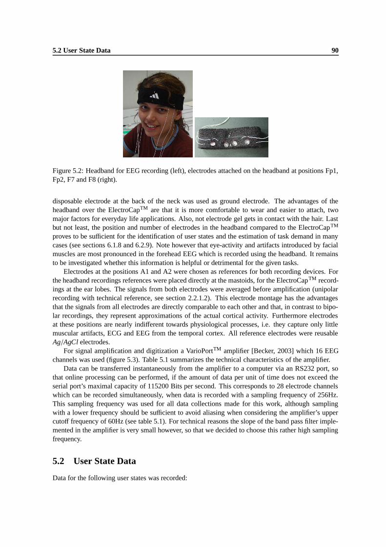
5.2 User State Data 90
Figure 5.2: Headband for EEG recording (left), electrodes attached on the headband at positions Fp1,Fp2, F7 and F8 (right).
disposable electrode at the back of the neck was used as ground electrode. The advantages of theheadband over the ElectroCapTM are that it is more comfortable to wear and easier to attach, twomajor factors for everyday life applications. Also, not electrode gel gets in contact with the hair. Lastbut not least, the position and number of electrodes in the headband compared to the ElectroCapTM
proves to be sufficient for the identification of user states and the estimation of task demand in manycases (see sections 6.1.8 and 6.2.9). Note however that eye-activity and artifacts introduced by facialmuscles are most pronounced in the forehead EEG which is recorded using the headband. It remainsto be investigated whether this information is helpful or detrimental for the given tasks.
Electrodes at the positions A1 and A2 were chosen as references for both recording devices. Forthe headband recordings references were placed directly at the mastoids, for the ElectroCapTM record-ings at the ear lobes. The signals from both electrodes were averaged before amplification (unipolarrecording with technical reference, see section 2.2.1.2). This electrode montage has the advantagesthat the signals from all electrodes are directly comparable to each other and that, in contrast to bipo-lar recordings, they represent approximations of the actual cortical activity. Furthermore electrodesat these positions are nearly indifferent towards physiological processes, i.e. they capture only littlemuscular artifacts, ECG and EEG from the temporal cortex. All reference electrodes were reusableAg/AgCl electrodes.
For signal amplification and digitization a VarioPortTM amplifier [Becker, 2003] which 16 EEGchannels was used (figure 5.3). Table 5.1 summarizes the technical characteristics of the amplifier.
Data can be transferred instantaneously from the amplifier to a computer via an RS232 port, sothat online processing can be performed, if the amount of data per unit of time does not exceed theserial port’s maximal capacity of 115200 Bits per second. This corresponds to 28 electrode channelswhich can be recorded simultaneously, when data is recorded with a sampling frequency of 256Hz.This sampling frequency was used for all data collections made for this work, although samplingwith a lower frequency should be sufficient to avoid aliasing when considering the amplifier’s uppercutoff frequency of 60Hz (see table 5.1). For technical reasons the slope of the band pass filter imple-mented in the amplifier is very small however, so that we decided to choose this rather high samplingfrequency.
5.2 User State Data
Data for the following user states was recorded:

5.2 User State Data 91
Amplification factor 2775Input Range ±450µVA/D conversion 12 Bit (4096 steps)Resolution 0,22 V / BitFrequency Range 0,9 ... 60 Hz
Table 5.1: Technical characteristics of the VarioportTM EEG amplifier used for data recording.
Figure 5.3: The VarioportTM EEG amplifier. Left: the actual amplifier, right: the recorder whichcontrols the amplifier, stores recorded data and established the connection to a computer.
Resting (R): Subjects were asked to relax and not to concentrate on a particular issue. Eyes had tostay open and most subjects preferred looking out of the window. Little to no background noisewas present during the resting periods, each lasting about 70 seconds.
The requirement to keep eyes open during the resting period should make sure that resting isnot simply identified by very pronounced α-activity in the EEG which can usually be observedonly in a relaxed state when eyes are closed. Instead a typical resting period during a meetingor a lecture should be simulated where eyes are not necessarily closed.
Listening to a talk (L): Subjects were given a talk, mostly about a medical topic, which containeda lot of facts to memorize and descriptions of complex processes, so that extensive use of theworking memory and visual imagination was required to be able to follow the talk. This is verycommon for talks where no additional visual information supporting the speech is available. Tomake sure that subjects listened attentively to the talk, they were asked to summarize its contentafterwards.
Perceiving an audio-visual presentation (P): A short presentation slide presentation was given abouta scientific topic with which the recorded subject was not familiar. Thus at least medium atten-tion was required to be able to understand the presentation. Images and graphical explanationsof facts were largely used to make sure that there were auditory and visual stimuli in contrastto user state listening. After the presentation subjects were asked to summarize it with the helpof the slides which should guarantee their attention during the presentation.
Reading an article (RE): An article from a popular news magazine of medium length (one to threepages) had to be read. Subjects were allowed to select an article which appeared interestingto them out of a large collection. This should make sure that they remembered the article wellenough to be able to summarize it afterwards.
Summarizing the read article (RS): Directly after reading, subjects had to summarize the read arti-cle. To facilitate this task and to enable subjects to talk long enough so that enough data couldbe collected, they were allowed to look from time to time at the text they had read before.

5.2 User State Data 92
Performing arithmetic operations (A): Arithmetic operations had to be performed on a sheet of pa-per. Depending on the mathematical background of the subjects, different tasks were selected:multiplications, divisions, summations and subtractions of four digit numbers, matrix multipli-cations or the computation of simple derivatives and integrals.
Not only the arithmetic task, but also the talk and the slide presentation were adapted to thebackground of the recorded subject, so that in all cases a reasonable amount of mental resourcesshould be required for task execution. This is important, since in cases of very low task demand, theneural correlates of different user states might be too weak (see section 2.3.2). Mental overload on theother hand might overwhelm the recorded subject and then lead to disengagement and thus again toweak EEG correlates of the currently recorded user state.
All user states were recorded consecutively. After each state or block of states (reading andsummarization of the read article are considered as block) there was a resting period. The orderof the other user states was chosen randomly in order to avoid biases in the data due to a fixed order.
When a classification function is trained, it is important to avoid biases due to non-equal amountof training data per class (see also section 4.5.1.5). This can either be done by balancing the trainingdata so that for each class approximately the same number of samples is available or by introducingweight factors for samples of different classes (similar to prior probabilities). Since the latter wasdifficult to integrate in the classifier implementations used for this work, we decided to balance thedata, thus accepting that some data had to be discarded.
As explained above, the resting periods lasted about 70 seconds only, while for the other userstates much more data per recording session was acquired. Therefore the data for user state restingwould be the limiting factor for amount of data per class after balancing. This problem was overcomeat least partly by concatenating for each session the data from two resting periods so that at least 140seconds of data from user state resting were available. Note that the duration of the resting periodscould have been increased as well, or more than two resting periods could have been concatenated.Subjects reported however that is was difficult to remain relaxed for a longer period then about 70seconds during the experiments, which excludes the possibility of recording longer resting periods.Concatenation of more than one resting period on the other hand would introduce more variability inthe data for user state resting only, thus making the system behave systematically different for thisuser state compared to the others1 . For these reasons we chose the compromise to concatenate onlytwo resting periods of 70 seconds length.
Data was collected from different subjects at different locations using either the ElectroCapTM
or the headband. All subjects were university students which volunteered for the experiments. Sub-jects were not paid for their participation. In the remainder of this thesis the following data sets aredistinguished for the user state data:
CMUSubjects: Six computer science students (four males, two females) between 23 and 33 yearsof age were recorded at Carnegie Mellon University in Pittsburgh (USA). None of them was anative English speaker, but they all had very good knowledge of the English language. 8767seconds of data in total were collected. In the following identifiers (U1), . . ., (U6) are used torefer to the recording sessions from the subjects of this data set.
UKASubjects: Three university students (two males, one female) with varying academic backgroundsbetween 23 and 26 years of age were recorded at University of Karlsruhe (Germany). One of
1Preliminary experiments have shown that classification accuracy increases for user state resting, when data from morethan one resting period (from the same recording session!) is contained in the test and training set.

5.2 User State Data 93
them was not a native German speaker. 9232 seconds of data are available from this datacollection. The UKASubjects recording sessions are referred to using the identifiers (U7a),(U7b), (U8a), (U8b) and (U9), where the letters ‘a’ and ‘b’ are used to distinguish the particularrecording sessions when one subject was recorded twice.
HeadBandSubjects: 3267 seconds of EEG data with the headband were collected at the Universityof Karlsruhe from two female university students with 21 and 23 years of age. The identifiers(U10) and (U11) refer to the two HeadBandSubjects recording sessions in the following.
Note that the amount of data in seconds given for the different data sets includes only EEG datarecorded for one of the six user states described above, i.e. only data which can actually be used forsubsequent processing. During the explanation of the recording procedure and during the time whichsubjects needed to prepare for the next state to be recorded no data was acquired.
In total data from eleven recordings with the ElectroCapTM and two recordings with the headbandare available. Table 5.2 shows for each user state the mean, the minimum and the maximum amountof data over all these recording sessions. In figure 5.4 this information is displayed separately foreach for the three data sets CMUSubjects, UKASubjects and HeadBandSubjects. Finally, in figure5.5 each recording session is considered separately and mean, minimum and maximum duration inseconds over all recorded user states is shown.
Two interesting observations can be made from table 5.2 and figures 5.4 and 5.5:
• The mean value for the state resting is lowest of all user states (see table 5.2 and figure 5.4),which suggests that the amount of data for this user state limits the size of the usable trainingdata per subject in many cases, since training sets are balanced. Indeed it can be seen from figure5.5 that the duration of the shortest user state is often around 140 seconds (which correspondsto the concatenation of two resting periods lasting about 70 seconds). Closer inspection of thedata from the different recording sessions reveals that the user state with this minimum durationis mostly resting. Remember that the amount of available data for this user state was alreadyenlarged by concatenating the data from two resting periods. For the reasons explained aboveno more data are available for that user state however.
• Furthermore it is interesting to compare the average durations of a recording session of thethree data sets: For the CMUSubjects data the average duration is 1461 seconds which issignificatnly less than the average duration for the UKASubjects data (1846 seconds) and theHeadBandSubjects data (1861 seconds). Furthermore it can be seen in figure 5.5 that the meanamount of data for one user state is smaller for the CMUSubjects recording sessions (sessions(U1), . . ., (U6)) compared to the other recording sessions (except sessions (U9) and (U10)).When looking at the single states, a significant difference in duration can be found for the statesperceiving a presentation (P) and summarizing the read article (RS).
As explanation for the difference for user state (P) might be, that for both data sets presenta-tions were held by a native German experimenter who talked German to the subjects whichwere recorded at Karlsruhe (UKASubjects and HeadBandSubjects data sets) and English tothe subjects which were recorded at Pittsburgh (CMUSubjects data set). Thus it is well pos-sible, that the experimenter was more brief in English than in his native language (where henaturally knows better to express himself), although for the English presentations exactly trans-lated versions of the German slides were used. A reason for the difference in duration for userstate (RS) could either be that the articles read by the subjects in Pittsburgh (from the ”TIME”magazine) were simply shorter than those read by the subjects in Karlsruhe (from the magazine

5.3 Task Demand Data 94
User State Mean Minimum Maximum
(R) 145 143 149(L) 264 169 388(P) 360 238 495
(RE) 408 223 646(RS) 206 124 345(A) 252 139 496
Complete session 1636 1267 2132
Table 5.2: Mean, minimum and maximum amount of data in seconds over all recording sessions foreach user state. In the last line mean, minimum and maximum length of a complete recording sessionare shown.
Figure 5.4: Mean amount for data in seconds for each user state over all recording sessions of the threedata sets CMUSubjects, UKASubjects and HeadBandSubjects. The shortest and longest durationof each state is depicted by the whiskers.
”Der Spiegel”). On the other hand it is possible that because of differences in style in both mag-azines, articles in the ”TIME” magazine contained less facts to report about than the articles of”Der Spiegel”.
5.3 Task Demand Data
Mental task demand data was collected while a 15 to 20 minutes long slide presentation with varyingdifficulty levels was given to the recorded subjects. During the presentation the laptop screen (slidesand mouse pointer) and the voice of the experimenter giving the presentation were recorded on a videotape. Directly after the presentation the recoded subjects were shown the video and asked to evaluate

5.3 Task Demand Data 95
Figure 5.5: Mean duration of one user state for each recording session. The duration of the shortestand longest state for each session is depicted by the whiskers.
their task demand over time which they experienced during the initial perception of the presentation.The following task demand levels could be chosen:
Low (L): It is possible to follow the presentation without any problems and without larger mentaleffort. Everything is understood, also details.
Medium (M): Some mental effort is required to be able to follow the presentation. Still everythingis understood, possibly except a few details.
High (H): Almost all available mental resources are required to be able to keep up with the pre-sentation. Details are mostly not understood anymore, however the essence of the presentedcontent is still clear. Task demand level high should also be chosen, if the talk is not understoodanymore, but still all mental resources are mobilized to try to understand it at least.
Overlad (O): The presentation is not understood anymore, the subject became overwhelmed, thendisengaged and makes no effort to gain the plot again.
The goal for the design of the presentations was that all task demand levels are experienced equallyby the recorded subjects during their perception. Since background knowledge of the subjects varieda lot, it was attempted to adapt topics and the way of their presentation individually for each subjectto reach that goal.
Many subjects reported that it was very difficult to estimate the own task demand which they ex-perienced during the initial perception of the presentation. Often they had difficulties to distinguishbetween their task demand during the presentation and during its video replay, and they were tempedto simply evaluate their current task demand while watching the video. Furthermore almost all sub-jects reported problems to find the exact transition between task demand level high and overload, i.e.the state where they still tried to understand the presentation but they could not and the state where

5.3 Task Demand Data 96
they became overwhelmed and therefore did not pay attention anymore. The question how reliablethe subjects’ self-estimates of task demand are, is addressed at the end of this section.
Two different task demand data sets were recorded at the University of Karlsruhe:
ElectroCapSubjects: In total 7690 seconds of task demand data were recorded using the ElectroCapTM.Six university students (three males, three females) with varying academic backgrounds be-tween 23 and 26 years of age volunteered for that data collection. Two subjects were none-native German speakers. The recording sessions from the different subjects of this data col-lection are referred to in the following using the identifiers (T1), . . ., (T6). One subject wasrecorded twice; the corresponding recording sessions are therefore identified with (T3a) and(T3b).
HeadBandSubjects: 1918 seconds of task demand data in total were collected from one male uni-versity student (28 years of age) and one female university student (21 years of age) usingthe headband. Both volunteered for the data collection, one subject was a non-native Germanspeaker. These recording sessions are assigned the identifiers (T7) and (T8).
Table 5.3 shows mean, minimum and maximum duration for the different task demand levels overall recording sessions. In figure 5.6 the duration of each task demand level, the mean duration ofone level and the total duration of the whole presentation is shown for each recording session. Notethat one task demand level could occur several times during the presentation. The durations of theparticular task demand levels displayed in table 5.3 and figure 5.6 result from the concatenation of alldata segments corresponding to the same level.
From the first column of table 5.3 one can see that the mean duration of 144 seconds for taskdemand level overload is the shortest of all task demand levels. It is in the same range as the meanduration of the user state for which in average least data is available, namely resting with 145 seconds(see table 5.2). The minimum durations of the different task demand levels (second column of table5.3) are however much shorter than those of the different user states (see table 5.2). This indicatesthat in general a balanced training set for task demand prediction contains less data than a balancedtraining set for user state identification. In figure 5.6 one can see that indeed for many recordingsessions much less than 145 seconds of data are available for at least one task demand level. This isnot the case for the user state data, where for one state at least 124 seconds and in most cases evenmore were recorded, see figure 5.5.
Note also the large fluctuations of the available data per task demand level for the different record-ing sessions which can be seen in figure 5.6. The goal for the design of the presentations to makesubjects experience each task demand level equally could not be reached. This shows, that it is ex-tremely difficult to anticipate the effects of a presentation on a listener, even if his or her backgroundknowledge is well known. Precisely this finding can serve as a hint, that EEG based task demandassessment can be very useful during a presentation in order to stay informed about changes in taskdemand of the audience or to be able to analyze the effect of the own talk later.
It was mentioned above that most subjects found it very difficult to estimate their task demandduring the initial perception of the presentation given the video replay. Therefore we wanted to findout how reliable their estimates are. This was done by asking the four subjects recorded in the sessions(T2), (T3b), (T4) and (T6) to repeat the evaluation of their task demand using the video a secondtime. These second evaluations took place two to eight weeks after the initial recording session. Thereason why the period between both evaluations was chosen to be sufficiently long was to avoid thatsubjects simply remembered and reproduced their decisions made during the first evaluation. Insteadsubjects were asked to estimate the task demand they experienced while watching the video, i.e.
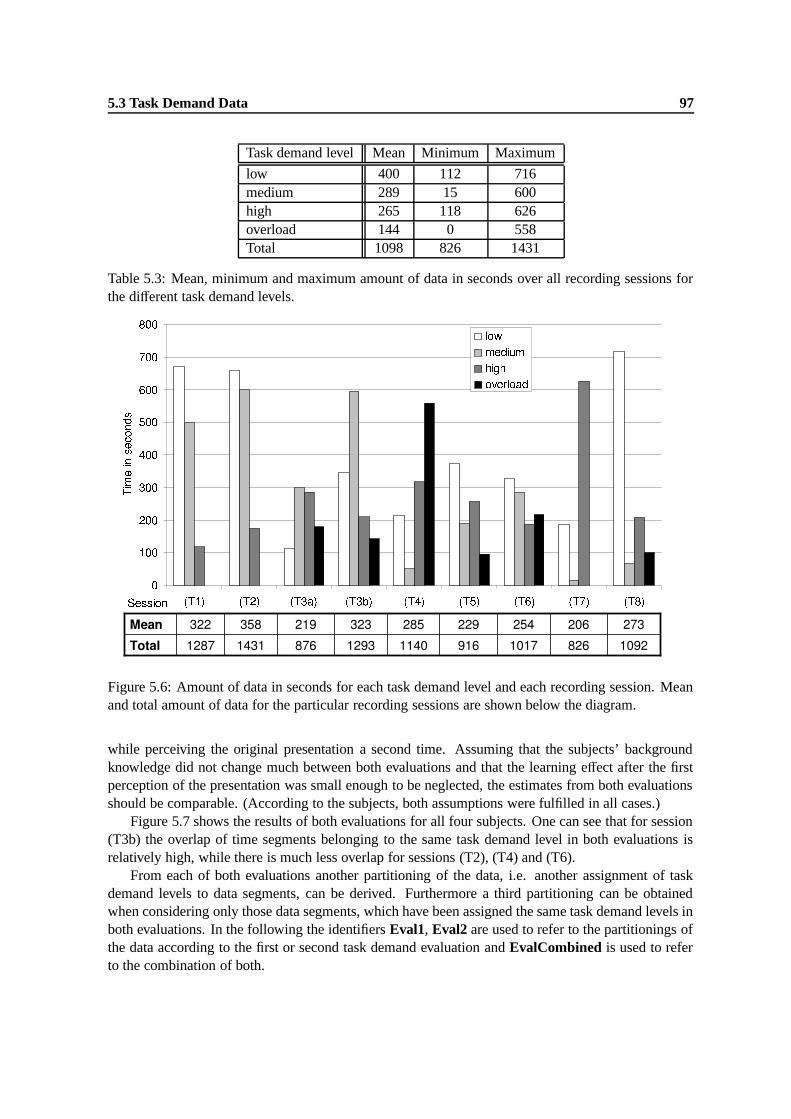
5.3 Task Demand Data 97
Task demand level Mean Minimum Maximum
low 400 112 716medium 289 15 600high 265 118 626overload 144 0 558Total 1098 826 1431
Table 5.3: Mean, minimum and maximum amount of data in seconds over all recording sessions forthe different task demand levels.
Figure 5.6: Amount of data in seconds for each task demand level and each recording session. Meanand total amount of data for the particular recording sessions are shown below the diagram.
while perceiving the original presentation a second time. Assuming that the subjects’ backgroundknowledge did not change much between both evaluations and that the learning effect after the firstperception of the presentation was small enough to be neglected, the estimates from both evaluationsshould be comparable. (According to the subjects, both assumptions were fulfilled in all cases.)
Figure 5.7 shows the results of both evaluations for all four subjects. One can see that for session(T3b) the overlap of time segments belonging to the same task demand level in both evaluations isrelatively high, while there is much less overlap for sessions (T2), (T4) and (T6).
From each of both evaluations another partitioning of the data, i.e. another assignment of taskdemand levels to data segments, can be derived. Furthermore a third partitioning can be obtainedwhen considering only those data segments, which have been assigned the same task demand levels inboth evaluations. In the following the identifiers Eval1, Eval2 are used to refer to the partitionings ofthe data according to the first or second task demand evaluation and EvalCombined is used to referto the combination of both.
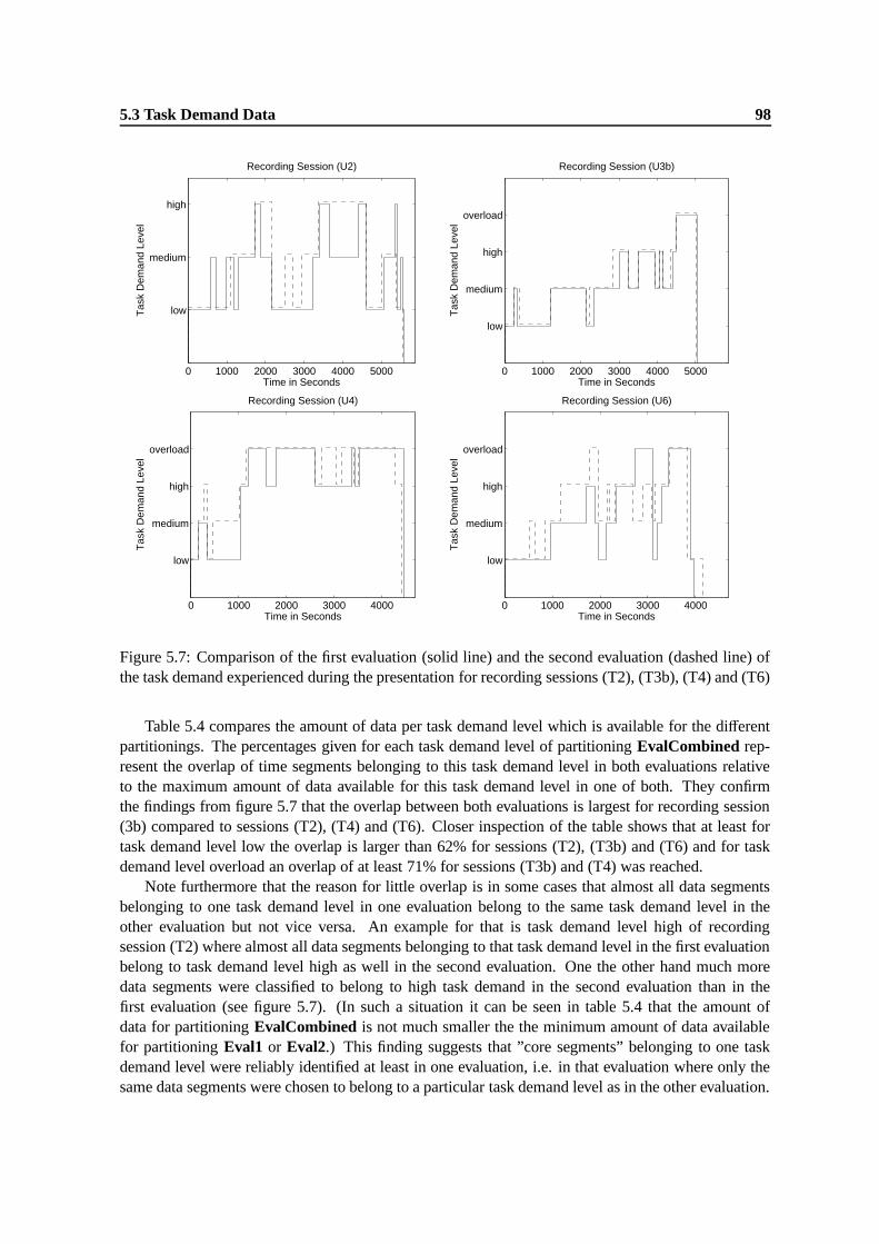
5.3 Task Demand Data 98
0 1000 2000 3000 4000 5000
low
medium
high
Time in Seconds
Tas
k D
eman
d Le
vel
Recording Session (U2)
0 1000 2000 3000 4000 5000
low
medium
high
overload
Time in Seconds
Tas
k D
eman
d Le
vel
Recording Session (U3b)
0 1000 2000 3000 4000
low
medium
high
overload
Time in Seconds
Tas
k D
eman
d Le
vel
Recording Session (U4)
0 1000 2000 3000 4000
low
medium
high
overload
Time in Seconds
Tas
k D
eman
d Le
vel
Recording Session (U6)
Figure 5.7: Comparison of the first evaluation (solid line) and the second evaluation (dashed line) ofthe task demand experienced during the presentation for recording sessions (T2), (T3b), (T4) and (T6)
Table 5.4 compares the amount of data per task demand level which is available for the differentpartitionings. The percentages given for each task demand level of partitioning EvalCombined rep-resent the overlap of time segments belonging to this task demand level in both evaluations relativeto the maximum amount of data available for this task demand level in one of both. They confirmthe findings from figure 5.7 that the overlap between both evaluations is largest for recording session(3b) compared to sessions (T2), (T4) and (T6). Closer inspection of the table shows that at least fortask demand level low the overlap is larger than 62% for sessions (T2), (T3b) and (T6) and for taskdemand level overload an overlap of at least 71% for sessions (T3b) and (T4) was reached.
Note furthermore that the reason for little overlap is in some cases that almost all data segmentsbelonging to one task demand level in one evaluation belong to the same task demand level in theother evaluation but not vice versa. An example for that is task demand level high of recordingsession (T2) where almost all data segments belonging to that task demand level in the first evaluationbelong to task demand level high as well in the second evaluation. One the other hand much moredata segments were classified to belong to high task demand in the second evaluation than in thefirst evaluation (see figure 5.7). (In such a situation it can be seen in table 5.4 that the amount ofdata for partitioning EvalCombined is not much smaller the the minimum amount of data availablefor partitioning Eval1 or Eval2.) This finding suggests that ”core segments” belonging to one taskdemand level were reliably identified at least in one evaluation, i.e. in that evaluation where only thesame data segments were chosen to belong to a particular task demand level as in the other evaluation.

5.3 Task Demand Data 99
Eval1 Eval2 EvalCombinedSession (L) (M) (H) (O) (L) (M) (H) (O) (L) (M) (H) (O)
(T2) 657 600 174 0 572 419 429 0 484(74%)
246(41%)
156(36%)
0
(T3b) 345 596 210 142 291 583 278 131 290(84%)
524(88%)
206(74%)
131(92%)
(T4) 213 51 318 558 70 169 185 707 67(31%)
25(15%)
115(36%)
504(71%)
(T6) 328 286 186 217 257 267 394 137 206(62%)
96(34%)
148(38%)
95(42%)
Table 5.4: Comparison of the amount of data in seconds available for each task demand level for datapartitionings Eval1, Eval2 and EvalCombined for recording sessions (T2), (T3b), (T4) and (T6). Thepercentages given for the last columns relate the amount of data per task demand level for partitioningEvalCombined to the maximum amount of data obtained from one of the partitionings Eval1 andEval2.
(In the above example this is the first evaluation.)An interesting question related to the overlapping segments of the same task demand level which
are contained in the partitioning EvalCombined in general, is whether predictions can be improvedwhen they are used for training and testing only. The underlying hypothesis here is that task demandestimates are more reliable for these segments, since they were assigned the same task demand levelin both evaluations. This hypothesis is further investigated in section 6.2.8.
The generally poor overlap indicates, how difficult it is to subjectively evaluate the own taskdemand during the perception of a presentation. This agrees as well with the comments of the recordedsubjects. Therefore it would not be too surprising, if training and test data were very noisy and featurevectors belonging to different task demand levels were very similar, so that the prediction of the correcttask demand level becomes extremely difficult.

Chapter 6
Experiments and Results
A lot of experiments have been conducted on the collected user state and task demand data, in orderto analyze the impact of the different processing steps on the whole system for user state identificationand task demand estimation and to optimize the overall system performance by configuring eachprocessing step appropriately. The results of these experiments are reported and discussed in thischapter using the performance measures introduced in chapter 4.6.
6.1 User State Identification
6.1.1 Experimental Setups
Several experimental setups are distinguished for the user state data in the following:
UD User and session dependent experiments: Data portions of the same recording session wereused for training (80% of the whole session), testing and validation (each 10% of the wholesession). All sessions from the CMUSubjectsdata collection (recording sessions (U1)-(U6))were used for this type of experiments. Training sets comprise here 668 seconds of data inaverage, validation sets 84 seconds and the test sets 146 seconds. If not indicated differently,results reported for this setup are always averages over the accuracies obtained for the test sets(or validation sets) of all recording sessions of this setup.
HB The same type of experiments as for setup UD were conducted on the HeadBandSubjects data(recording sessions (U10) and (U11)). The average training set length is here 681 seconds,the validation set length 84 seconds and the test set length 163 seconds. Also here usuallyaverages over the test set (or validation set) results from both recording sessions are reported inthe following.
UI User independent experiments: For the CMUSubjects data collection the system was trainedon data from five recording sessions (in average 3338 seconds of training data) and tested ondata from the remaining session in a round-robin manner. For comparability of the results thesame test sets as for setup UD were used and results are reported as averages over all recordingsessions as above. For validation 1082 seconds of data from the sessions (U7a), (U8a) and(U9) from the UKASubjects data collection were available. If results for a particular recordingsession are given for this setup in the following, the session number refers always to that sessionfrom which the test data is taken.

6.1 User State Identification 101
SI User dependent but session independent experiments: For the subjects from the UKASubjectsdata set which were recorded twice (recording sessions (U7a), (U7b), (U8a) and (U8b)) thesystem was trained using 80% of the the data of one session (in average 672 seconds) and testedon the 10% of the data recorded from the same subject in the other session (in average 198seconds). Thus there are always results from 4 test sets available for averaging in the following.Note that for this setup no good validation data exists. For the early stopping regularizationmethod for ANNs 10% of data from the training sessions were used which bears the risk ofoverfitting however and does not reflect the properties of a real session independent experimen-tal setup. For these reasons and since the data from the test session must not be touched forvalidation (this comes too close to parameter tuning on the test set), no cross validation wasapplied to determine system parameters for setup SI. Instead parameter values were chosenwhich are somewhere in-between the parameters estimated for setups UD and UI following theintuition that properties of setup SI are in-between those of the other two setups.
Note that the length of the different data sets in seconds corresponds to the number of featurevectors per data set, since features are extracted from two seconds long time windows which overlapone second as explained in section 4.2. Note furthermore that the fraction of data for training has beenbalanced after its extraction. That applies to the validation set, too, however not for the test set whichdoes not have to be balanced for the reasons explained in section 4.6. This also explains why theavailable amount of data is different for validation and testing, even when originally the same fractionof data was extracted for both.
As described above for setups UD and UI exactly the same test sets were used, which allows directcomparison of the results. In contrast to that the test sets for setups SI and HB are both based on datafrom other recording sessions. This has to be taken into account when comparing the results obtainedfor these setups with others. For this reason accuracies obtained for setups UD and UI are clearlyseparated from those obtained for setup SI or setup HB in the following sections.
6.1.2 ANN topology selection
Before ANN-based classifiers can be trained and used to make predictions, their topology, i.e. thenumber of hidden layers and the number of neurons per hidden layer, must be determined. If thetopology can not be inferred from a priori knowledge, this is usually done using cross-validation. Theabove described validation sets however are already required for early stopping regularization (seesection 4.5.1.5). Therefore training, validation and test data from recording sessions (U7a), (U8a)and (U9) (the ”validation sessions” of setup UI) was taken to determine the network topology forsetup UD. For setup UI additional data from the same sessions which is however not contained inthe original validation sets was used for topology selection. (The original training sets were kepthere.) No topology selection was performed for setup SI, because no appropriate validation data wasavailable for this setup as explained above. Since ANNs with one hidden layer are suitable for mostclassification problems in practice, cross-validation was used here only to determine the number ofhidden units for a network with a single hidden layer.
Figure 6.1 shows the accuracies obtained for the topology selection data sets of setup UD andsetup UI for different numbers of hidden units. One can see that for both setups the fluctuations ofaccuracies are very small. In particular they are smaller than the standard deviations (depicted by thewhiskers) over five repetitions of the same experiments. Note that these standard deviations are stillhigh (in particular for setup UI), although for each of the five experiments five networks were trainedwith the same data and a majority decision over the predictions of all networks was made to obtain
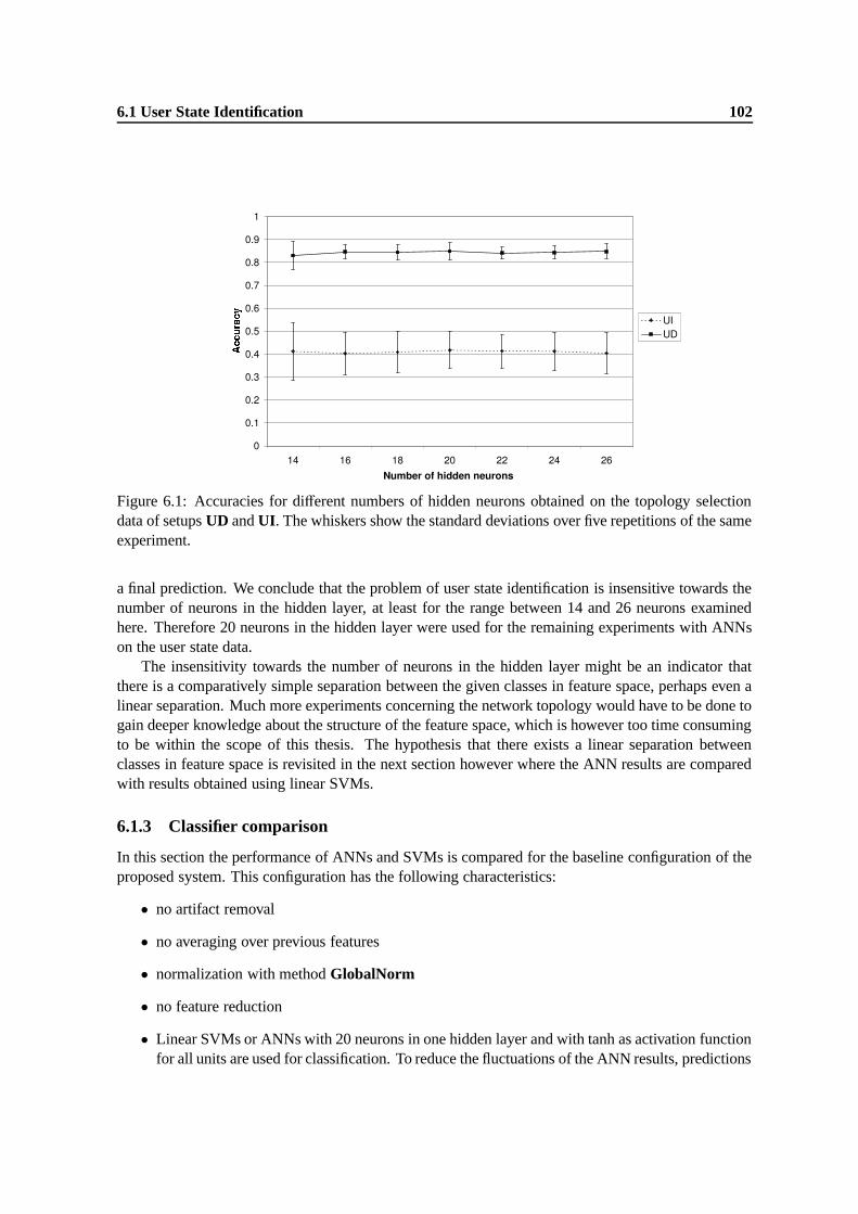
6.1 User State Identification 102
Figure 6.1: Accuracies for different numbers of hidden neurons obtained on the topology selectiondata of setups UD and UI. The whiskers show the standard deviations over five repetitions of the sameexperiment.
a final prediction. We conclude that the problem of user state identification is insensitive towards thenumber of neurons in the hidden layer, at least for the range between 14 and 26 neurons examinedhere. Therefore 20 neurons in the hidden layer were used for the remaining experiments with ANNson the user state data.
The insensitivity towards the number of neurons in the hidden layer might be an indicator thatthere is a comparatively simple separation between the given classes in feature space, perhaps even alinear separation. Much more experiments concerning the network topology would have to be done togain deeper knowledge about the structure of the feature space, which is however too time consumingto be within the scope of this thesis. The hypothesis that there exists a linear separation betweenclasses in feature space is revisited in the next section however where the ANN results are comparedwith results obtained using linear SVMs.
6.1.3 Classifier comparison
In this section the performance of ANNs and SVMs is compared for the baseline configuration of theproposed system. This configuration has the following characteristics:
• no artifact removal
• no averaging over previous features
• normalization with method GlobalNorm
• no feature reduction
• Linear SVMs or ANNs with 20 neurons in one hidden layer and with tanh as activation functionfor all units are used for classification. To reduce the fluctuations of the ANN results, predictions
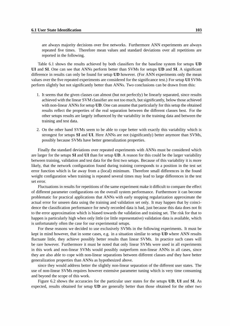
6.1 User State Identification 103
are always majority decisions over five networks. Furthermore ANN experiments are alwaysrepeated five times. Therefore mean values and standard deviations over all repetitions arereported in the following.
Table 6.1 shows the results achieved by both classifiers for the baseline system for setups UDUI and SI. One can see that ANNs perform better than SVMs for setups UD and SI. A significantdifference in results can only be found for setup UD however. (For ANN experiments only the meanvalues over the five repeated experiments are considered for the significance test.) For setup UI SVMsperform slightly but not significantly better than ANNs. Two conclusions can be drawn from this:
1. It seems that the given classes can almost (but not perfectly) be linearly separated, since resultsachieved with the linear SVM classifier are not too much, but significantly, below those achievedwith non-linear ANNs for setup UD. One can assume that particularly for this setup the obtainedresults reflect the properties of the real separation between the different classes best. For theother setups results are largely influenced by the variability in the training data and between thetraining and test data.
2. On the other hand SVMs seem to be able to cope better with exactly this variability which isstrongest for setups SI and UI. Here ANNs are not (significantly) better anymore than SVMs,possibly because SVMs have better generalization properties.
Finally the standard deviations over repeated experiments with ANNs must be considered whichare larger for the setups SI and UI than for setup UD. A reason for this could be the larger variabilitybetween training, validation and test data for the first two setups. Because of this variability it is morelikely, that the network configuration found during training corresponds to a position in the test seterror function which is far away from a (local) minimum. Therefore small differences in the foundweight configuration when training is repeated several times may lead to large differences in the testset error.
Fluctuations in results for repetitions of the same experiment make it difficult to compare the effectof different parameter configurations on the overall system performance. Furthermore it can becomeproblematic for practical applications that ANNs with early stopping regularization approximate theactual error for unseen data using the training and validation set only. It may happen that by coinci-dence the classification performance for newly recorded data is bad, just because this data does not fitto the error approximation which is biased towards the validation and training set. The risk for that tohappen is particularly high when only little (or little representative) validation data is available, whichis unfortunately often the case for our experimental setups.
For these reasons we decided to use exclusively SVMs in the following experiments. It must bekept in mind however, that in some cases, e.g. in a situation similar to setup UD where ANN resultsfluctuate little, they achieve possibly better results than linear SVMs. In practice such cases willbe rare however. Furthermore it must be noted that only linear SVMs were used in all experimentsin this work and non-linear SVMs would possibly outperform non-linear ANNs in all cases, sincethey are also able to cope with non-linear separations between different classes and they have bettergeneralization properties than ANNs as hypothesized above.
since they would address better the slightly non-linear separation of the different user states. Theuse of non-linear SVMs requires however extensive parameter tuning which is very time consumingand beyond the scope of this work.
Figure 6.2 shows the accuracies for the particular user states for the setups UD, UI and SI. Asexpected, results obtained for setup UD are generally better than those obtained for the other two
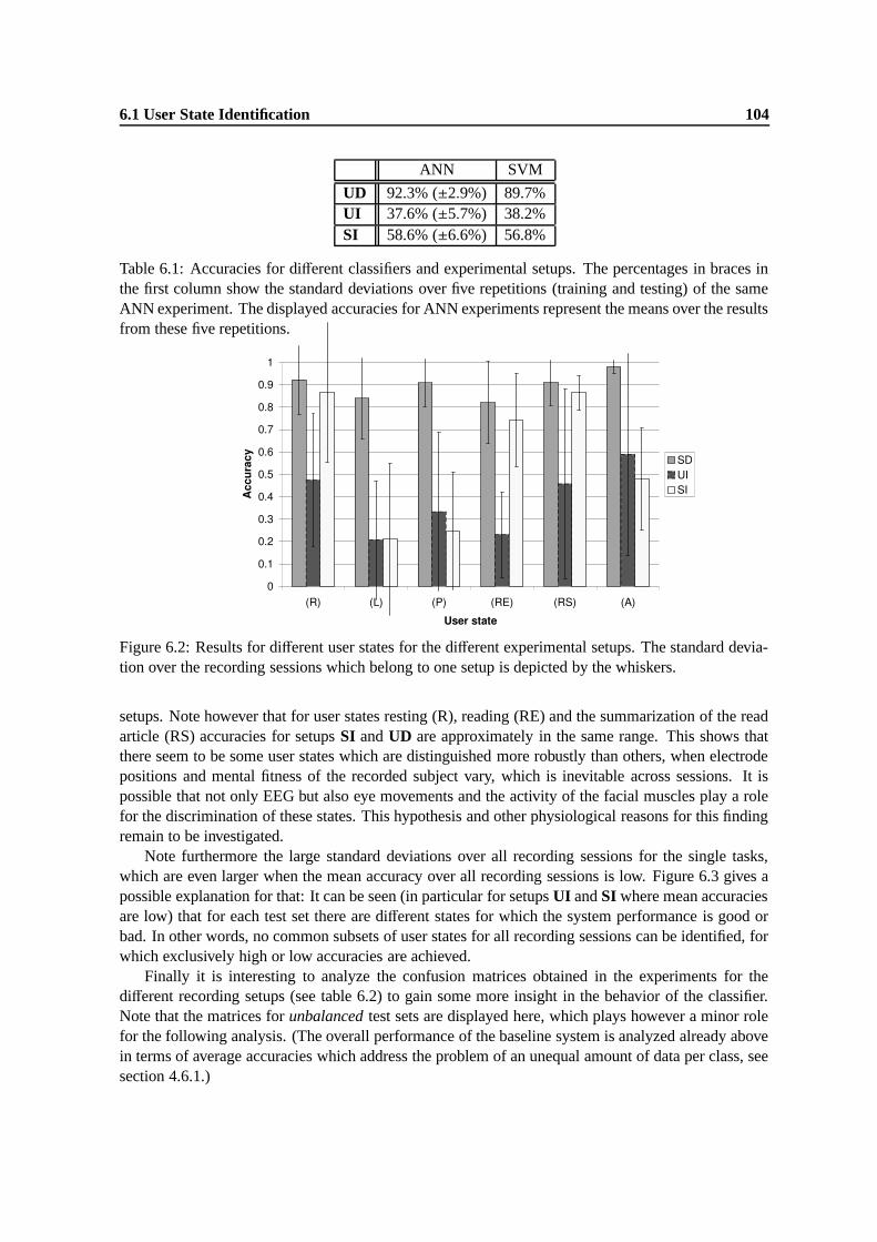
6.1 User State Identification 104
ANN SVM
UD 92.3% (±2.9%) 89.7%UI 37.6% (±5.7%) 38.2%SI 58.6% (±6.6%) 56.8%
Table 6.1: Accuracies for different classifiers and experimental setups. The percentages in braces inthe first column show the standard deviations over five repetitions (training and testing) of the sameANN experiment. The displayed accuracies for ANN experiments represent the means over the resultsfrom these five repetitions.
Figure 6.2: Results for different user states for the different experimental setups. The standard devia-tion over the recording sessions which belong to one setup is depicted by the whiskers.
setups. Note however that for user states resting (R), reading (RE) and the summarization of the readarticle (RS) accuracies for setups SI and UD are approximately in the same range. This shows thatthere seem to be some user states which are distinguished more robustly than others, when electrodepositions and mental fitness of the recorded subject vary, which is inevitable across sessions. It ispossible that not only EEG but also eye movements and the activity of the facial muscles play a rolefor the discrimination of these states. This hypothesis and other physiological reasons for this findingremain to be investigated.
Note furthermore the large standard deviations over all recording sessions for the single tasks,which are even larger when the mean accuracy over all recording sessions is low. Figure 6.3 gives apossible explanation for that: It can be seen (in particular for setups UI and SI where mean accuraciesare low) that for each test set there are different states for which the system performance is good orbad. In other words, no common subsets of user states for all recording sessions can be identified, forwhich exclusively high or low accuracies are achieved.
Finally it is interesting to analyze the confusion matrices obtained in the experiments for thedifferent recording setups (see table 6.2) to gain some more insight in the behavior of the classifier.Note that the matrices for unbalanced test sets are displayed here, which plays however a minor rolefor the following analysis. (The overall performance of the baseline system is analyzed already abovein terms of average accuracies which address the problem of an unequal amount of data per class, seesection 4.6.1.)
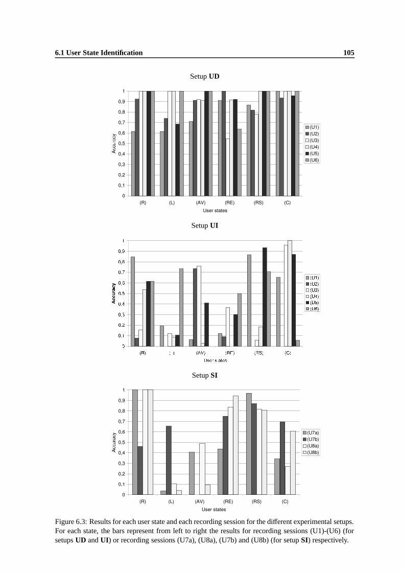
6.1 User State Identification 105
Setup UD
Setup UI
Setup SI
Figure 6.3: Results for each user state and each recording session for the different experimental setups.For each state, the bars represent from left to right the results for recording sessions (U1)-(U6) (forsetups UD and UI) or recording sessions (U7a), (U8a), (U7b) and (U8b) (for setup SI) respectively.
6.1 User State Identification 106
While for setup UD the largest entries of the confusion matrix are found on the main diagonal,this is not anymore the case for setups UI and SI where moderately high values are spread all overthe matrices. This is not surprising when the accuracies achieved for the different setups (see table6.1) are taken into account. User states which are confused particularly often for setups UI and SI areanalyzed now.
For both setups the states listening (L) and perceiving a presentation (P) are often confused withresting (R). A reason for that could be natural fluctuations in alertness during the states (L) and (P),i.e. subjects can not stay constantly alert for several minutes while listening to a talk or perceiving apresentation. Furthermore the basic alertness level during state (R) varies across subjects and sessions.Therefore it becomes likely that a short lapse in alertness during states (L) or (P) is classified as resting(R) for setups UI or SI, since for one or more training sessions recorded from subjects with a highbasic alertness level, a similar activity pattern could have been observed during state (R).
Next, it can be seen that state (L) is often confused with state (P) for setups UI and SI and state(P) is often confused with state (L) for setup SI and with state (A) for setup UI. This can possibly beexplained with the fact that similar cortex regions are activated for states (L), (P) and (A) (see alsosection 2.3.1): All three states require the understanding of symbols (letters, numbers) which involvesthe parietal cortex. Furthermore states (P) and (L) require the processing of speech and languagewhich takes places in the temporal cortex. Therefore possibly only small differences in the EEGbetween the particular states exist, which are still sufficient for their discrimination in case of setupUD, but not anymore in case of the other two setups due to the variability across sessions and subjects.
Finally the arithmetics state (A) is often confused with reading (RE) for setup SI and the state (RE)is often confused with states (P) and (A) for setup UI. The same explanation as given before mighthold here as well, since in all cases the parietal cortex for the understanding of symbols is stronglyinvolved.
6.1.4 Averaging
The first attempt to improve the performance of the baseline system was to apply averaging overthe previous k feature vectors (see section 4.2.2). The optimal value of k was obtained using crossvalidation. We consider a value of k to be optimal here, when improvements achieved by increasingit even more remain small compared to the improvements obtained before. The accuracies on thevalidation sets for different values of k are shown in figure 6.4 for setups UD and UI.
While for setup UD there are no considerable improvements for k > 2 anymore, the accuracy forsetup UI improves up to k = 4. Therefore the following experiments were continued with values ofkopt = 2 for setup UD, with kopt = 4 for setup UI and with kopt = 3 for setup SI. The value of kopt forsetup SI was chosen, following the reasoning from section 6.1.1 that properties of this experimentalsetup lie somewhere in-between those for the other two setups. Table 6.3 compares the baselineresults (k = 1) with those which are obtained when averaging over the kopt previous feature vectors isperformed for the test data of the different experimental setups. In all cases significant improvementsfor k = kopt are achieved compared to the baseline system.
It is interesting that different values of kopt are found for the different setups. This can possiblyagain be explained with the different degree of noise and variability contained in the data of the differ-ent setups. When using slack variables, an SVM is able to cope with a certain amount of variabilityand noise in the data. While for setup UD the SVMs have to cope only with the natural temporalfluctuations of the EEG signal, for setup UI additional variability is introduced by the individual dif-ferences in the EEG data of the subjects in the training set. Therefore the influence of the temporalsignal fluctuations has to be reduced more for this setup which is done by choosing a larger value of

6.1 User State Identification 107
Setup UDPrediction
(R) (L) (P) (RE) (RS) (A)
(R 72 4 0 1 1 0(L) 9 124 8 1 4 0
Target (P) 5 5 151 1 2 4(RE) 12 1 21 181 3 3(RS) 0 1 0 5 79 2(A) 0 0 1 0 1 120
Setup UIPrediction
(R) (L) (P) (RE) (RS) (A)
(R) 37 9 14 10 4 4(L) 49 34 33 14 10 6
Target (P) 45 9 56 17 3 38(RE) 23 10 43 53 16 76(RS) 3 6 16 5 42 15(A) 0 0 18 23 3 78
Setup SIPrediction
(R) (L) (P) (RE) (RS) (A)
(R) 45 7 0 0 0 0(L) 44 24 17 8 7 7
Target (P) 53 55 42 14 4 1(RE) 1 22 0 141 2 31(RS) 0 3 1 8 86 0(A) 1 1 1 71 2 56
Table 6.2: Confusion matrices for the different recording setups. The displayed matrices represent thesum over the confusion matrices of all test sets of one recording setup.
k, i.e. by considering a larger context. Thus the classifier is able to address other types of variability.When the considered context is too large however, a change of user state might be detected with delayonly, since at the time where the new user state begins too many samples of the old user state are stilltaken into account.
6.1.5 Normalization
Up two this point, all reported results were obtained using the baseline normalization method Glob-alNorm which performs mean subtraction and variance normalization globally for the whole data,using mean and variance estimates from the complete training set. As we have seen in the previoussections, the variability between subjects or sessions for setups UI and SI seems to be detrimental tothe classification results. One possibility to address that problem which is investigated in this section,is to use normalization method UserNorm, where mean subtraction and variance normalization isperformed separately for each recording session contained in the training, validation or test set. Fur-
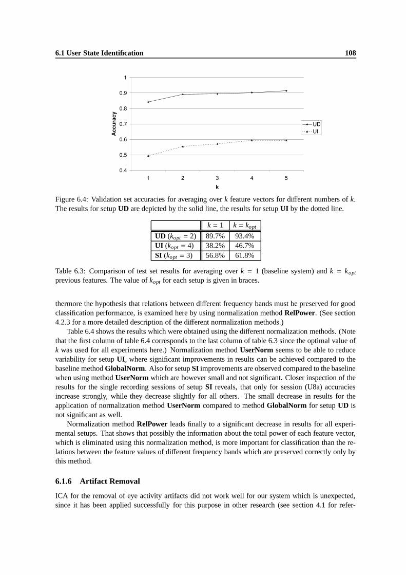
6.1 User State Identification 108
Figure 6.4: Validation set accuracies for averaging over k feature vectors for different numbers of k.The results for setup UD are depicted by the solid line, the results for setup UI by the dotted line.
k = 1 k = kopt
UD (kopt = 2) 89.7% 93.4%UI (kopt = 4) 38.2% 46.7%SI (kopt = 3) 56.8% 61.8%
Table 6.3: Comparison of test set results for averaging over k = 1 (baseline system) and k = kopt
previous features. The value of kopt for each setup is given in braces.
thermore the hypothesis that relations between different frequency bands must be preserved for goodclassification performance, is examined here by using normalization method RelPower. (See section4.2.3 for a more detailed description of the different normalization methods.)
Table 6.4 shows the results which were obtained using the different normalization methods. (Notethat the first column of table 6.4 corresponds to the last column of table 6.3 since the optimal value ofk was used for all experiments here.) Normalization method UserNorm seems to be able to reducevariability for setup UI, where significant improvements in results can be achieved compared to thebaseline method GlobalNorm. Also for setup SI improvements are observed compared to the baselinewhen using method UserNorm which are however small and not significant. Closer inspection of theresults for the single recording sessions of setup SI reveals, that only for session (U8a) accuraciesincrease strongly, while they decrease slightly for all others. The small decrease in results for theapplication of normalization method UserNorm compared to method GlobalNorm for setup UD isnot significant as well.
Normalization method RelPower leads finally to a significant decrease in results for all experi-mental setups. That shows that possibly the information about the total power of each feature vector,which is eliminated using this normalization method, is more important for classification than the re-lations between the feature values of different frequency bands which are preserved correctly only bythis method.
6.1.6 Artifact Removal
ICA for the removal of eye activity artifacts did not work well for our system which is unexpected,since it has been applied successfully for this purpose in other research (see section 4.1 for refer-
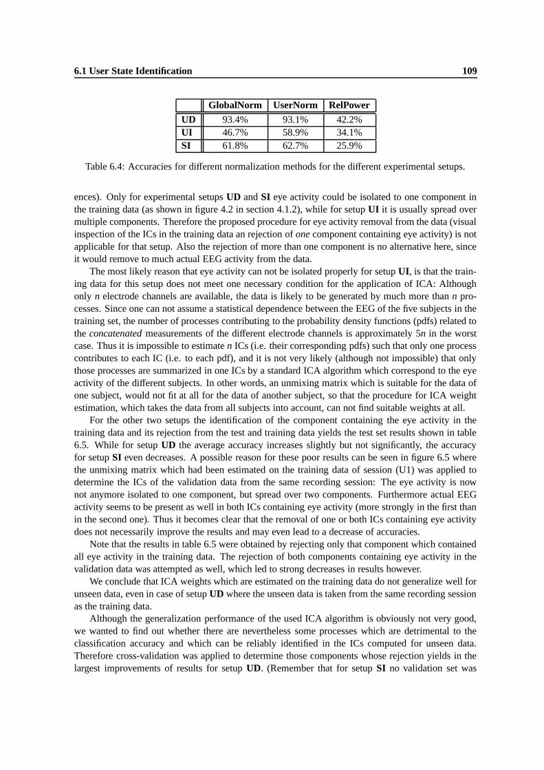
6.1 User State Identification 109
GlobalNorm UserNorm RelPower
UD 93.4% 93.1% 42.2%UI 46.7% 58.9% 34.1%SI 61.8% 62.7% 25.9%
Table 6.4: Accuracies for different normalization methods for the different experimental setups.
ences). Only for experimental setups UD and SI eye activity could be isolated to one component inthe training data (as shown in figure 4.2 in section 4.1.2), while for setup UI it is usually spread overmultiple components. Therefore the proposed procedure for eye activity removal from the data (visualinspection of the ICs in the training data an rejection of one component containing eye activity) is notapplicable for that setup. Also the rejection of more than one component is no alternative here, sinceit would remove to much actual EEG activity from the data.
The most likely reason that eye activity can not be isolated properly for setup UI, is that the train-ing data for this setup does not meet one necessary condition for the application of ICA: Althoughonly n electrode channels are available, the data is likely to be generated by much more than n pro-cesses. Since one can not assume a statistical dependence between the EEG of the five subjects in thetraining set, the number of processes contributing to the probability density functions (pdfs) related tothe concatenated measurements of the different electrode channels is approximately 5n in the worstcase. Thus it is impossible to estimate n ICs (i.e. their corresponding pdfs) such that only one processcontributes to each IC (i.e. to each pdf), and it is not very likely (although not impossible) that onlythose processes are summarized in one ICs by a standard ICA algorithm which correspond to the eyeactivity of the different subjects. In other words, an unmixing matrix which is suitable for the data ofone subject, would not fit at all for the data of another subject, so that the procedure for ICA weightestimation, which takes the data from all subjects into account, can not find suitable weights at all.
For the other two setups the identification of the component containing the eye activity in thetraining data and its rejection from the test and training data yields the test set results shown in table6.5. While for setup UD the average accuracy increases slightly but not significantly, the accuracyfor setup SI even decreases. A possible reason for these poor results can be seen in figure 6.5 wherethe unmixing matrix which had been estimated on the training data of session (U1) was applied todetermine the ICs of the validation data from the same recording session: The eye activity is nownot anymore isolated to one component, but spread over two components. Furthermore actual EEGactivity seems to be present as well in both ICs containing eye activity (more strongly in the first thanin the second one). Thus it becomes clear that the removal of one or both ICs containing eye activitydoes not necessarily improve the results and may even lead to a decrease of accuracies.
Note that the results in table 6.5 were obtained by rejecting only that component which containedall eye activity in the training data. The rejection of both components containing eye activity in thevalidation data was attempted as well, which led to strong decreases in results however.
We conclude that ICA weights which are estimated on the training data do not generalize well forunseen data, even in case of setup UD where the unseen data is taken from the same recording sessionas the training data.
Although the generalization performance of the used ICA algorithm is obviously not very good,we wanted to find out whether there are nevertheless some processes which are detrimental to theclassification accuracy and which can be reliably identified in the ICs computed for unseen data.Therefore cross-validation was applied to determine those components whose rejection yields in thelargest improvements of results for setup UD. (Remember that for setup SI no validation set was
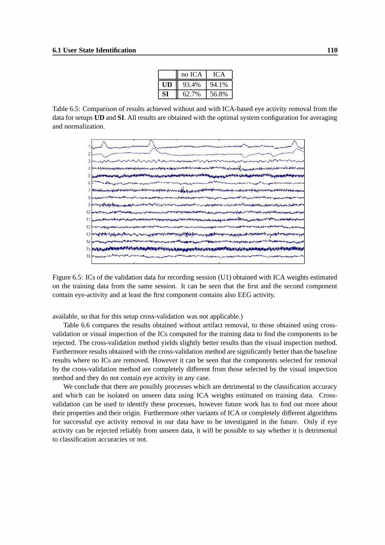
6.1 User State Identification 110
no ICA ICA
UD 93.4% 94.1%SI 62.7% 56.8%
Table 6.5: Comparison of results achieved without and with ICA-based eye activity removal from thedata for setups UD and SI. All results are obtained with the optimal system configuration for averagingand normalization.
Figure 6.5: ICs of the validation data for recording session (U1) obtained with ICA weights estimatedon the training data from the same session. It can be seen that the first and the second componentcontain eye-activity and at least the first component contains also EEG activity.
available, so that for this setup cross-validation was not applicable.)Table 6.6 compares the results obtained without artifact removal, to those obtained using cross-
validation or visual inspection of the ICs computed for the training data to find the components to berejected. The cross-validation method yields slightly better results than the visual inspection method.Furthermore results obtained with the cross-validation method are significantly better than the baselineresults where no ICs are removed. However it can be seen that the components selected for removalby the cross-validation method are completely different from those selected by the visual inspectionmethod and they do not contain eye activity in any case.
We conclude that there are possibly processes which are detrimental to the classification accuracyand which can be isolated on unseen data using ICA weights estimated on training data. Cross-validation can be used to identify these processes, however future work has to find out more abouttheir properties and their origin. Furthermore other variants of ICA or completely different algorithmsfor successful eye activity removal in our data have to be investigated in the future. Only if eyeactivity can be rejected reliably from unseen data, it will be possible to say whether it is detrimentalto classification accuracies or not.

6.1 User State Identification 111
Session no ICA vis. inspection cross validation
(U1) 86.4% 1 92.1% 3 92.3%(U2) 93.2% - 93.2% 9 94.2%(U3) 95.7% 3 93.5% 8 97.1%(U4) 97.6% 2 97.8% 12 97.6%(U5) 92.8% 3 92.4% 10 93.8%(U6) 94.7% 5 95.5% 16 94.7%Total 93.4% 94.1% 94.9%
Table 6.6: Comparison of results for the different recording sessions obtained without ICA to thoseobtained using ICA and visual inspection of the training data or cross-validation to find the compo-nents to be rejected. Left of the results for a particular method the number of the component which isrejected for each recording session is shown. A dash denotes that no component has been rejected.
6.1.7 Feature Reduction
Two potential feature reduction methods which are applicable for classification problems were pre-sented in section 4.3: Averaging over adjacent frequency bands (referred to as FreqAvg method in thissection) and linear discriminant analysis (LDA).
Figure 6.6 shows the validation set accuracies for setups UD and UI when adjacent features are puttogether in bins of size b, i.e. when averaging over b adjacent frequency bands is performed. In bothcases no significant increase in results can be observed for any value of b, but results remain stablewith increasing bin size for a while. For setup UD results start to decrease for with bin size of about12 which corresponds to a total feature vector dimensionality of 128 features. (Note that the originalfeature vector dimensionality was 1440.) For setup UI results decrease already for b = 7 where intotal 208 features are used. A very interesting observation is that results decrease only moderately upto b = 45 for both setups. In this case only two features per electrode are considered anymore: theaverage power for the lower frequencies (1-22 Hz) and the higher frequencies (23-45 Hz). Only forb = 90 (one feature per electrode) results drop strongly. This supports the hypothesis from section2.3.1 that for each electrode information about the total power in the lower frequency range (aroundthe α-band) and in the higher frequency range (around the 40Hz γ-activity) is sufficient to distinguishdifferent user states.
As explained in section 4.3.2, LDA coefficients can only be estimated when enough data is avail-able, since otherwise the eigenvalue problem to solve is ill-conditioned. Therefore LDA can only beapplied for setup UI here. Figure 6.7 shows the validation set accuracies for LDA-based dimension-ality reduction to different feature vector sizes.
For LDA-based feature reduction accuracies start to drop already for larger feature vector sizescompared to the FreqAvg method. Furthermore it can be seen that for the latter the accuracy for setupUI is still larger than 50% when only two features per electrode are considered (32 features in total),while the accuracy for LDA-based feature reduction to the same number of features is significantlylower. Closer inspection of the features selected by LDA for this feature vector size reveals thatpreferably very low frequency bands are selected, especially the bands 0 - 0.5Hz and 0.5 - 1Hz (seetable 6.8) and that across training sets there is a strong overlap between the selected features. Asexplained in section 2.3.1 these low frequencies correspond to DC potentials which are related to theprocessing of sensory inputs. They are usually pertubed with sweating and electrode artifacts howeverand therefore attenuated by the amplifiers. Nonetheless LDA seems to be able to extract valuableinformation from these features. A reason that LDA performs worse than the FreqAvg method might
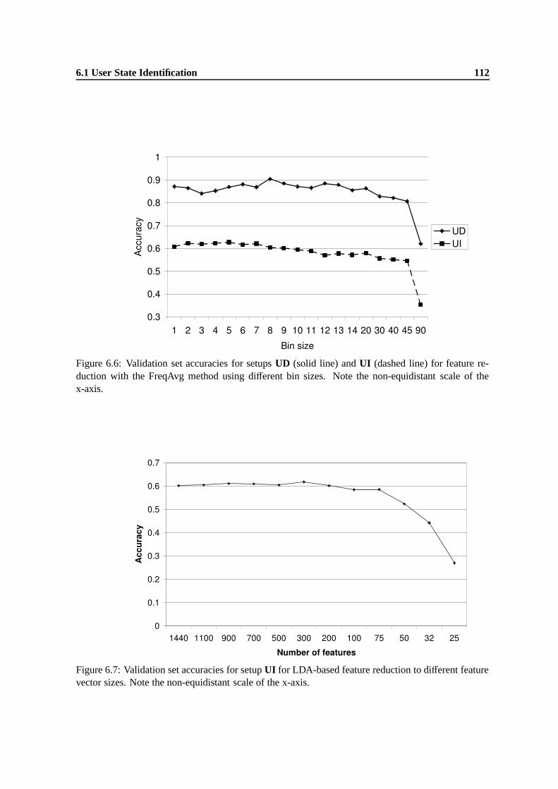
6.1 User State Identification 112
Figure 6.6: Validation set accuracies for setups UD (solid line) and UI (dashed line) for feature re-duction with the FreqAvg method using different bin sizes. Note the non-equidistant scale of thex-axis.
Figure 6.7: Validation set accuracies for setup UI for LDA-based feature reduction to different featurevector sizes. Note the non-equidistant scale of the x-axis.

6.1 User State Identification 113
Setup No feat. reduction LDA FreqAvg
UD 93.4% - 93.0% (144, b = 10)UI 58.9% 57.5% (300) 53.1% (288, b = 5)SI 62.7% - 62.5% (205, b = 7)
Table 6.7: Results for feature reduction on the test data for the different experimental setups usingLDA and the FreqAvg method compared to the baseline results obtained without feature reduction. Adash indicates that no results are available for a particular case. The number of features (and the valueof b where applicable) are displayed in braces. For better comparability no ICA was used for setupUD although this might improve results slightly. All results are obtained with the optimal systemconfiguration for averaging and normalization determined in the previous sections.
be that LDA imposes a linear separation between the classes which seems not to be true completelyalthough linear SVMs achieve comparatively good classification results (see also section 6.1.3).
One common reason for the application of feature reduction is that the elimination of features in-troducing only noise in the data might lead to better overall results. From figures 6.6 and 6.7 it can beseen that feature reduction can not improve results here. A possible explanation is that the classifieritself is well able to cope with noise, because it selects a separation between the classes where noisyfeatures play a minor role. Another advantage of feature vector dimensionality reduction is howeverthat statistical models can be estimated more reliably, even when only little data is available. Further-more less memory is required to store learned models and training and classification procedures mayspeed up a lot when the number of used features is reduced.
For these reasons it is interesting whether a feature vector dimensionality can be determined fromthe validation set results, so that results remain stable but the number of features is reduced signifi-cantly for unseen data. We decided here to make conservative choices for the reduced feature vectordimensionalities, i.e. they were chosen sufficiently larger then those dimensionalities where validationset results start to drop. Thus it should be more likely to obtain stable test set results.
Table 6.7 compares the test set results for both feature reduction methods (the feature vectordimensionality has been determined from the validation data as described above) with the baselinewhere no feature reduction is performed. All results drop slightly (but not significantly) compared tothe baseline, however it can still be said that they remain stable. The only exception are the resultsobtained with feature reduction method FreqAvg for setup UI, where a significant decrease in resultsis observed. Possibly the choice of b = 5 from the validation data was not conservative enough, i.e.possibly the validation data does not reflect the properties of the test set well enough in this case.
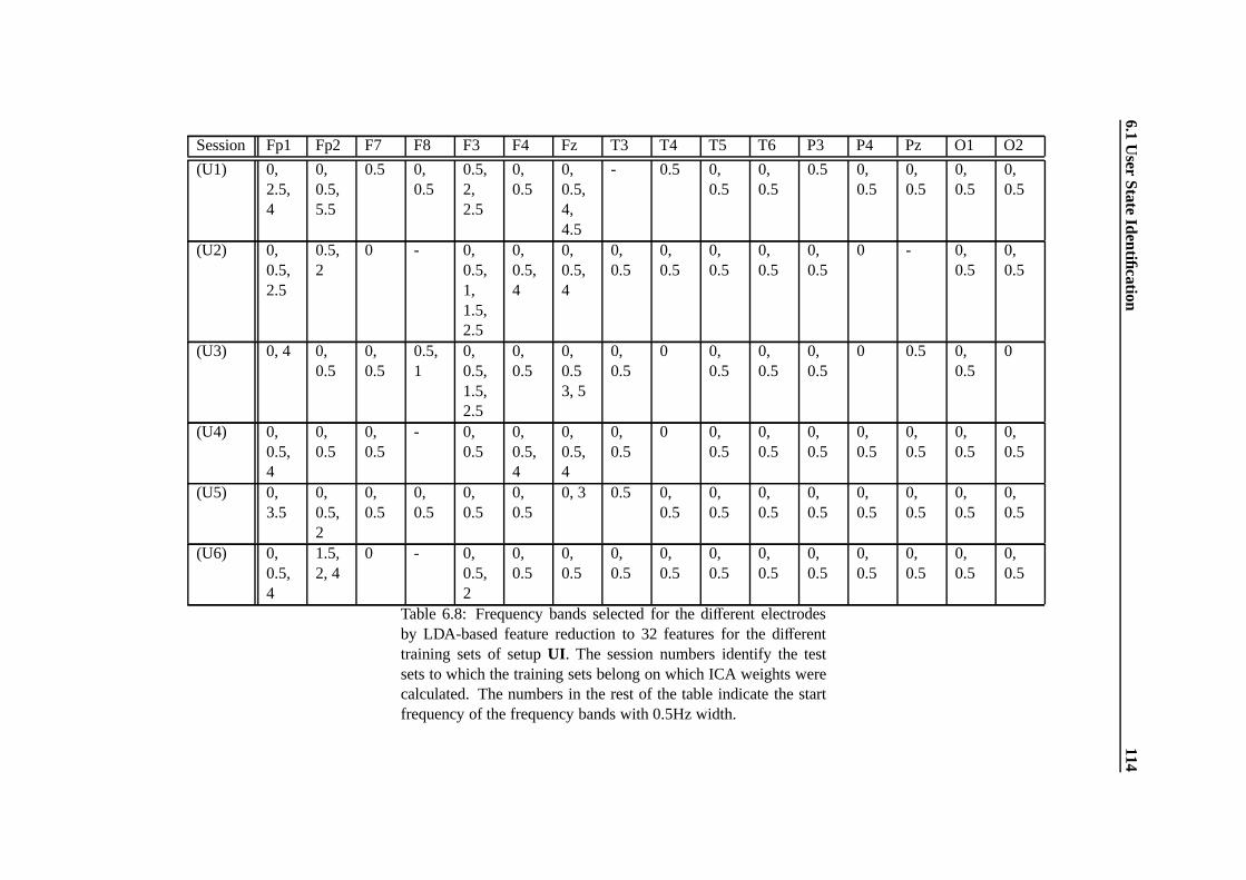
6.1U
serState
Identification114
Session Fp1 Fp2 F7 F8 F3 F4 Fz T3 T4 T5 T6 P3 P4 Pz O1 O2
(U1) 0,2.5,4
0,0.5,5.5
0.5 0,0.5
0.5,2,2.5
0,0.5
0,0.5,4,4.5
- 0.5 0,0.5
0,0.5
0.5 0,0.5
0,0.5
0,0.5
0,0.5
(U2) 0,0.5,2.5
0.5,2
0 - 0,0.5,1,1.5,2.5
0,0.5,4
0,0.5,4
0,0.5
0,0.5
0,0.5
0,0.5
0,0.5
0 - 0,0.5
0,0.5
(U3) 0, 4 0,0.5
0,0.5
0.5,1
0,0.5,1.5,2.5
0,0.5
0,0.53, 5
0,0.5
0 0,0.5
0,0.5
0,0.5
0 0.5 0,0.5
0
(U4) 0,0.5,4
0,0.5
0,0.5
- 0,0.5
0,0.5,4
0,0.5,4
0,0.5
0 0,0.5
0,0.5
0,0.5
0,0.5
0,0.5
0,0.5
0,0.5
(U5) 0,3.5
0,0.5,2
0,0.5
0,0.5
0,0.5
0,0.5
0, 3 0.5 0,0.5
0,0.5
0,0.5
0,0.5
0,0.5
0,0.5
0,0.5
0,0.5
(U6) 0,0.5,4
1.5,2, 4
0 - 0,0.5,2
0,0.5
0,0.5
0,0.5
0,0.5
0,0.5
0,0.5
0,0.5
0,0.5
0,0.5
0,0.5
0,0.5
Table 6.8: Frequency bands selected for the different electrodesby LDA-based feature reduction to 32 features for the differenttraining sets of setup UI. The session numbers identify the testsets to which the training sets belong on which ICA weights werecalculated. The numbers in the rest of the table indicate the startfrequency of the frequency bands with 0.5Hz width.
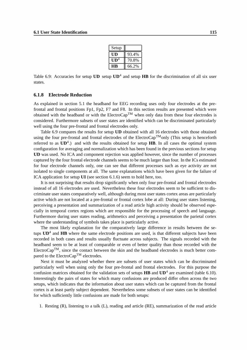
6.1 User State Identification 115
Setup
UD 93.4%UD4 70.8%HB 66.2%
Table 6.9: Accuracies for setup UD setup UD4 and setup HB for the discrimination of all six userstates.
6.1.8 Electrode Reduction
As explained in section 5.1 the headband for EEG recording uses only four electrodes at the pre-frontal and frontal positions Fp1, Fp2, F7 and F8. In this section results are presented which wereobtained with the headband or with the ElectroCapTM when only data from these four electrodes isconsidered. Furthermore subsets of user states are identified which can be discriminated particularlywell using the four pre-frontal and frontal electrodes only.
Table 6.9 compares the results for setup UD obtained with all 16 electrodes with those obtainedusing the four pre-frontal and frontal electrodes of the ElectroCapTMonly (This setup is henceforthreferred to as UD4.) and with the results obtained for setup HB. In all cases the optimal systemconfiguration for averaging and normalization which has been found in the previous sections for setupUD was used. No ICA and component rejection was applied however, since the number of processescaptured by the four frontal electrode channels seems to be much larger than four. In the ICs estimatedfor four electrode channels only, one can see that different processes such as eye activity are notisolated to single components at all. The same explanations which have been given for the failure ofICA application for setup UI (see section 6.1.6) seem to hold here, too.
It is not surprising that results drop significantly when only four pre-frontal and frontal electrodesinstead of all 16 electrodes are used. Nevertheless these four electrodes seem to be sufficient to dis-criminate user states comparatively well, although during most user states cortex areas are particularlyactive which are not located at a pre-frontal or frontal cortex lobe at all: During user states listening,perceiving a presentation and summarization of a read article high activity should be observed espe-cially in temporal cortex regions which are responsible for the processing of speech and language.Furthermore during user states reading, arithmetics and perceiving a presentation the parietal cortexwhere the understanding of symbols takes place is particularly active.
The most likely explanation for the comparatively large difference in results between the se-tups UD4 and HB where the same electrode positions are used, is that different subjects have beenrecorded in both cases and results usually fluctuate across subjects. The signals recorded with theheadband seem to be at least of comparable or even of better quality than those recorded with theElectroCapTM, since the contact between the skin and the headband electrodes is much better com-pared to the ElectroCapTM electrodes.
Next it must be analyzed whether there are subsets of user states which can be discriminatedparticularly well when using only the four pre-frontal and frontal electrodes. For this purpose theconfusion matrices obtained for the validation sets of setups HB and UD4 are examined (table 6.10).Interestingly the pairs of states for which many confusions are produced differ often across the twosetups, which indicates that the information about user states which can be captured from the frontalcortex is at least partly subject dependent. Nevertheless some subsets of user states can be identifiedfor which sufficiently little confusions are made for both setups:
1. Resting (R), listening to a talk (L), reading and article (RE), summarization of the read article
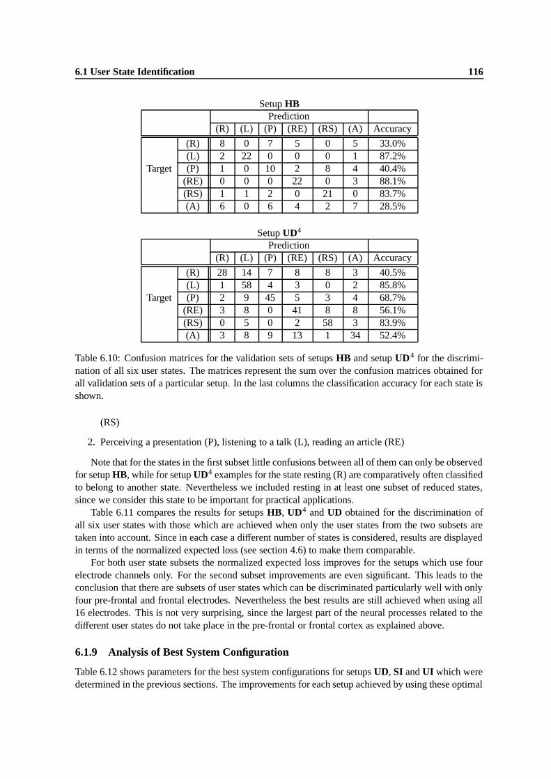
6.1 User State Identification 116
Setup HBPrediction
(R) (L) (P) (RE) (RS) (A) Accuracy
(R) 8 0 7 5 0 5 33.0%(L) 2 22 0 0 0 1 87.2%
Target (P) 1 0 10 2 8 4 40.4%(RE) 0 0 0 22 0 3 88.1%(RS) 1 1 2 0 21 0 83.7%(A) 6 0 6 4 2 7 28.5%
Setup UD4
Prediction(R) (L) (P) (RE) (RS) (A) Accuracy
(R) 28 14 7 8 8 3 40.5%(L) 1 58 4 3 0 2 85.8%
Target (P) 2 9 45 5 3 4 68.7%(RE) 3 8 0 41 8 8 56.1%(RS) 0 5 0 2 58 3 83.9%(A) 3 8 9 13 1 34 52.4%
Table 6.10: Confusion matrices for the validation sets of setups HB and setup UD4 for the discrimi-nation of all six user states. The matrices represent the sum over the confusion matrices obtained forall validation sets of a particular setup. In the last columns the classification accuracy for each state isshown.
(RS)
2. Perceiving a presentation (P), listening to a talk (L), reading an article (RE)
Note that for the states in the first subset little confusions between all of them can only be observedfor setup HB, while for setup UD4 examples for the state resting (R) are comparatively often classifiedto belong to another state. Nevertheless we included resting in at least one subset of reduced states,since we consider this state to be important for practical applications.
Table 6.11 compares the results for setups HB, UD4 and UD obtained for the discrimination ofall six user states with those which are achieved when only the user states from the two subsets aretaken into account. Since in each case a different number of states is considered, results are displayedin terms of the normalized expected loss (see section 4.6) to make them comparable.
For both user state subsets the normalized expected loss improves for the setups which use fourelectrode channels only. For the second subset improvements are even significant. This leads to theconclusion that there are subsets of user states which can be discriminated particularly well with onlyfour pre-frontal and frontal electrodes. Nevertheless the best results are still achieved when using all16 electrodes. This is not very surprising, since the largest part of the neural processes related to thedifferent user states do not take place in the pre-frontal or frontal cortex as explained above.
6.1.9 Analysis of Best System Configuration
Table 6.12 shows parameters for the best system configurations for setups UD, SI and UI which weredetermined in the previous sections. The improvements for each setup achieved by using these optimal
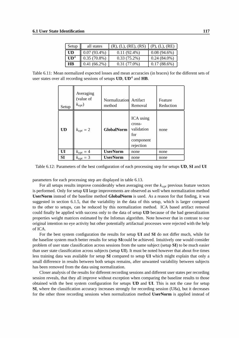
6.1 User State Identification 117
Setup all states (R), (L), (RE), (RS) (P), (L), (RE)
UD 0.07 (93.4%) 0.11 (92.4%) 0.08 (94.6%)UD4 0.35 (70.8%) 0.33 (75.2%) 0.24 (84.0%)HB 0.41 (66.2%) 0.31 (77.0%) 0.17 (88.6%)
Table 6.11: Mean normalized expected losses and mean accuracies (in braces) for the different sets ofuser states over all recording sessions of setups UD, UD4 and HB.
Setup
Averaging(value ofkopt)
Normalizationmethod
ArtifactRemoval
FeatureReduction
UD kopt = 2 GlobalNorm
ICA usingcross-validationforcomponentrejection
none
UI kopt = 4 UserNorm none noneSI kopt = 3 UserNorm none none
Table 6.12: Parameters of the best configuration of each processing step for setups UD, SI and UI
parameters for each processing step are displayed in table 6.13.For all setups results improve considerably when averaging over the kopt previous feature vectors
is performed. Only for setup UI large improvements are observed as well when normalization methodUserNorm instead of the baseline method GlobalNorm is used. As a reason for that finding, it wassuggested in section 6.1.5, that the variability in the data of this setup, which is larger comparedto the other to setups, can be reduced by this normalization method. ICA based artifact removalcould finally be applied with success only to the data of setup UD because of the bad generalizationproperties weight matrices estimated by the Infomax algorithm. Note however that in contrast to ouroriginal intention no eye activity but other potentially artifactual processes were rejected with the helpof ICA.
For the best system configuration the results for setup UI and SI do not differ much, while forthe baseline system much better results for setup SIcould be achieved. Intuitively one would considerproblem of user state classification across sessions from the same subject (setup SI) to be much easierthan user state classification across subjects (setup UI). It must be noted however that about five timesless training data was available for setup SI compared to setup UI which might explain that only asmall difference in results between both setups remains, after unwanted variability between subjectshas been removed from the data using normalization.
Closer analysis of the results for different recording sessions and different user states per recordingsession reveals, that they all improve without exception when comparing the baseline results to thoseobtained with the best system configuration for setups UD and UI. This is not the case for setupSI, where the classification accuracy increases strongly for recording session (U8a), but it decreasesfor the other three recording sessions when normalization method UserNorm is applied instead of
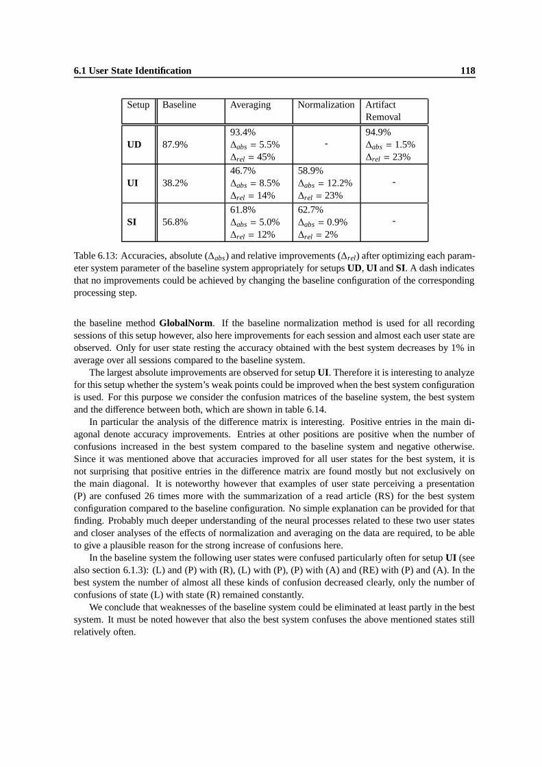
6.1 User State Identification 118
Setup Baseline Averaging Normalization ArtifactRemoval
UD 87.9%93.4%∆abs = 5.5%∆rel = 45%
-94.9%∆abs = 1.5%∆rel = 23%
UI 38.2%46.7%∆abs = 8.5%∆rel = 14%
58.9%∆abs = 12.2%∆rel = 23%
-
SI 56.8%61.8%∆abs = 5.0%∆rel = 12%
62.7%∆abs = 0.9%∆rel = 2%
-
Table 6.13: Accuracies, absolute (∆abs) and relative improvements (∆rel) after optimizing each param-eter system parameter of the baseline system appropriately for setups UD, UI and SI. A dash indicatesthat no improvements could be achieved by changing the baseline configuration of the correspondingprocessing step.
the baseline method GlobalNorm. If the baseline normalization method is used for all recordingsessions of this setup however, also here improvements for each session and almost each user state areobserved. Only for user state resting the accuracy obtained with the best system decreases by 1% inaverage over all sessions compared to the baseline system.
The largest absolute improvements are observed for setup UI. Therefore it is interesting to analyzefor this setup whether the system’s weak points could be improved when the best system configurationis used. For this purpose we consider the confusion matrices of the baseline system, the best systemand the difference between both, which are shown in table 6.14.
In particular the analysis of the difference matrix is interesting. Positive entries in the main di-agonal denote accuracy improvements. Entries at other positions are positive when the number ofconfusions increased in the best system compared to the baseline system and negative otherwise.Since it was mentioned above that accuracies improved for all user states for the best system, it isnot surprising that positive entries in the difference matrix are found mostly but not exclusively onthe main diagonal. It is noteworthy however that examples of user state perceiving a presentation(P) are confused 26 times more with the summarization of a read article (RS) for the best systemconfiguration compared to the baseline configuration. No simple explanation can be provided for thatfinding. Probably much deeper understanding of the neural processes related to these two user statesand closer analyses of the effects of normalization and averaging on the data are required, to be ableto give a plausible reason for the strong increase of confusions here.
In the baseline system the following user states were confused particularly often for setup UI (seealso section 6.1.3): (L) and (P) with (R), (L) with (P), (P) with (A) and (RE) with (P) and (A). In thebest system the number of almost all these kinds of confusion decreased clearly, only the number ofconfusions of state (L) with state (R) remained constantly.
We conclude that weaknesses of the baseline system could be eliminated at least partly in the bestsystem. It must be noted however that also the best system confuses the above mentioned states stillrelatively often.

6.1 User State Identification 119
Setup UI, baseline configurationPrediction
(R) (L) (P) (RE) (RS) (A)
(R) 37 9 14 10 4 4(L) 49 34 33 14 10 6
Target (P) 45 9 56 17 3 38(RE) 23 10 43 53 16 76(RS) 3 6 16 5 42 15(A) 0 0 18 23 3 78
Setup UI, best configurationPrediction
(R) (L) (P) (RE) (RS) (A)
(R) 44 16 10 5 3 0(L) 49 65 25 0 4 3
Target (P) 31 14 77 10 29 7(RE) 34 15 29 100 11 32(RS) 4 0 4 3 73 3(A) 0 0 8 14 8 92
Difference between best and baseline configuration for setup UIPrediction
(R) (L) (P) (RE) (RS) (A)
(R) 7 7 -4 -5 -1 -4(L) 0 31 -8 -14 -6 -3
Target (P) -14 5 21 -7 26 -31(RE) 11 5 -14 47 -5 -44(RS) 1 -6 -12 -2 31 -12(A) 0 0 -10 -9 5 14
Table 6.14: Confusion matrices of the baseline system, the best system and the difference betweenboth for setup UI.
6.1.10 Prototype System
To show the feasibility of user state classification in real time and to be able to get an immediateresponse of the system when data is recorded under different conditions, a prototype system has beendeveloped (figure 6.8).
The workflow of the system can be described as follows: First raw EEG data is acquired with theheadband and the amplifier which are described in section 5.1. Then a Pentium III 800MHz laptopis used for data processing. Data is received by the computer via the serial RS232 port using a C++-based data acquisition tool which has been developed at University of Karlsruhe. Then preprocessingand classification are performed with a MATLABTM implementation of the corresponding algorithms(which is partly based on standard tool boxes). Finally a hypothesis for the current user state isdisplayed by the data acquisition tool. Note that for technical reasons ANNs instead of SVMs areused as classifiers in the prototype system.
EEG is recorded continuously and every five seconds a new user state hypothesis is produced
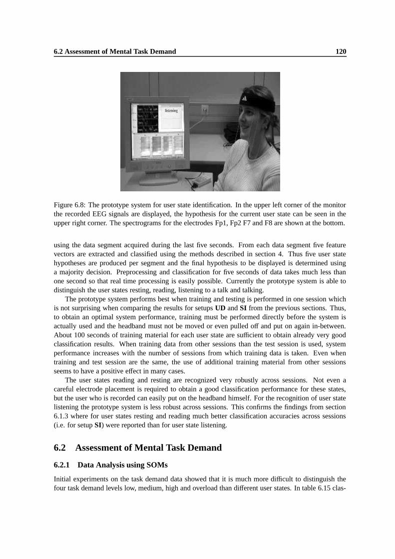
6.2 Assessment of Mental Task Demand 120
Figure 6.8: The prototype system for user state identification. In the upper left corner of the monitorthe recorded EEG signals are displayed, the hypothesis for the current user state can be seen in theupper right corner. The spectrograms for the electrodes Fp1, Fp2 F7 and F8 are shown at the bottom.
using the data segment acquired during the last five seconds. From each data segment five featurevectors are extracted and classified using the methods described in section 4. Thus five user statehypotheses are produced per segment and the final hypothesis to be displayed is determined usinga majority decision. Preprocessing and classification for five seconds of data takes much less thanone second so that real time processing is easily possible. Currently the prototype system is able todistinguish the user states resting, reading, listening to a talk and talking.
The prototype system performs best when training and testing is performed in one session whichis not surprising when comparing the results for setups UD and SI from the previous sections. Thus,to obtain an optimal system performance, training must be performed directly before the system isactually used and the headband must not be moved or even pulled off and put on again in-between.About 100 seconds of training material for each user state are sufficient to obtain already very goodclassification results. When training data from other sessions than the test session is used, systemperformance increases with the number of sessions from which training data is taken. Even whentraining and test session are the same, the use of additional training material from other sessionsseems to have a positive effect in many cases.
The user states reading and resting are recognized very robustly across sessions. Not even acareful electrode placement is required to obtain a good classification performance for these states,but the user who is recorded can easily put on the headband himself. For the recognition of user statelistening the prototype system is less robust across sessions. This confirms the findings from section6.1.3 where for user states resting and reading much better classification accuracies across sessions(i.e. for setup SI) were reported than for user state listening.
6.2 Assessment of Mental Task Demand
6.2.1 Data Analysis using SOMs
Initial experiments on the task demand data showed that it is much more difficult to distinguish thefour task demand levels low, medium, high and overload than different user states. In table 6.15 clas-

6.2 Assessment of Mental Task Demand 121
Session Low Medium High Overload Average Norm. expt. loss
(T1) 62% 27% 100% - 63% 0.56(T2) 44% 39% 100% - 61% 0.59(T3a) 90% 0% 40% 88% 53% 0.72(T4) 75% 100% 10% 0% 46% 0.61
Table 6.15: Accuracies for each task demand level obtained in an initial subject and session dependentexperiment for recording sessions (T1), (T2), (T3a) and (T4). Linear multiclass SVMs were used asclassifiers here, for averaging a value of k = 2 was chosen and normalization was performed withmethod GlobalNorm. A dash at a certain position indicates that no data for that task demand levelfrom the corresponding recording session was available.
sification accuracies for the discrimination of the task demand levels low, medium, high and overloadare shown for recording sessions (T1), (T2), (T3a) and (T4). An experimental setup similar to setupUD for the user state data was used to obtain these results: Classification was performed with linearmulticlass SVMs, for averaging a value of k = 2 was chosen and normalization method GlobalNormwas applied.
The obtained accuracies are all above the chance accuracy of 25%, however far below the resultswhich were obtained for setup UDfor the discrimination of six user states. Furthermore it can be seenfrom table 6.15 that for each recording session there are no more than two task demand levels forwhich the accuracies are clearly above chance. Closer inspection of the confusion matrices for thesinlge recording sessions reveals, that the examples for task demand levels with low accuracies aremostly classified to belong to one task demand level with a higher accuracy.
Also when using ANNs for classification or the regression versions of SVMs or ANNs results cannot be improved. This leads to the hypotheses that either the neural correlates of task demand whichcan be measured in the EEG are too weak to be used for the prediction of task demand, or that thetarget values for the available data are too unreliable. Especially the latter hypothesis seems plausible,since the targets were obtained from subjective task demand evaluations by the recorded subjects ,and subjects usually found it very difficult to identify the exact transition between two levels of taskdemand (see section 5.3). This hypothesis is supported even more when considering the poor overlapbetween time segments corresponding to the same task demand level for two subjective evaluationsof one recording (see table 5.4).
To find out whether there is at least some structure in the data despite the potentially bad quality ofthe references, i.e. to find out whether there are at least two or three task demand levels which can bereliably discriminated, SOMs were trained to gain insight about the spatial relations of the availablefeature vectors. Only if all feature vectors belonging to different task demand levels are sufficientlyfar away from each other, the training of classification or regression functions for the discriminationof these task demand levels makes sense.
Figure 6.9 shows the SOMs for recording sessions (T1), (T2), (T3a) and (T4). After SOM training,the BMUs of the examples belonging to different task demand levels were indicated in the map asdots of different colors. The size of the dots is proportional to the number of examples of one taskdemand level sharing the same BMU. To make the generation of the SOMs computationally tractable,averaging over five adjacent frequency bands was performed which should not be too detrimental tothe results according to the experience with the user state data (see section 6.1.7). (In section 6.2.7 it isconfirmed that also results for the task demand data remain stable, even when averaging is performedover up to 45 adjacent features.)

6.2 Assessment of Mental Task Demand 122
The BMUs for task demand level medium overlap either with those for task demand level high(in case of session (T2)), with those for task demand level low (in case of session (T4)) or even withthe BMUs for task demand level high and low (in case of sessions (T1) and (T3a)). This agrees withthe above hypothesis that either the EEG activity related to medium task demand is not very differentfrom the activity related to low or high task demand, or that subjects were simply not able to find theexact transitions between medium task demand and the other task demand levels. Since in table 6.15the lowest accuracies are reported also for task demand level medium, we decided to exclude it fromfurther experiments.
Only for two of the four considered recording sessions (sessions (T3a) and (T4)) examples for taskdemand level overload are available, and it can be seen from figure 6.9 that their corresponding BMUsalmost do not overlap with the BMUs of other task demand levels. For session (T4) however no clearseparation between the BMUs for the examples of task demand levels high and overload can be seen,which suggests bad generalization performance for unseen data. To analyze the relation between thethree remaining task demand levels low, high and overload in greater detail, SOMs for sessions (T3a)and (T4) were trained with examples for these task demand levels only (see figure 6.10). Now someoverlap between the BMUs for examples of task demand levels high and overload can be seen forsession (T3a), while for session (T4) there is still no overlap but also no clear separation betweenthe BMUs of examples of both task demand levels. The finding for session (T3a) that overload andhigh task demand are only separated well in the SOM trained on all data (figure 6.9) suggests, thatthe feature vectors of both two task demand levels belong to separate clusters which are however veryclose together. As a consequence of that for unseen data generalization might be bad. Furthermoreit can be found for the initial experiments described above that either many confusions were madebetween high task demand and overload (in case of session (T3a)) or that examples of task demandlevel overload were exclusively classified to belong to other arbitrary task demand levels (in case forsession (T4)). For these reasons also examples of task demand level overload were excluded from thefollowing experiments.
Figure 6.11 shows finally the SOMs for the four recording sessions which are trained only on theexamples for the remaining task demand levels low and high. Except for session (T1), one can see thatexamples for low and high task demand have mostly to non-overlapping BMUs which are separatedclearly in the SOMs. This indicates that also for unseen data the prediction of these two task demandlevels should work well. The overlapping BMUs of both task demand levels for session (T1) suggestthat the variance between feature vectors for different task demand levels is smaller than the variancewithin the group for feature vectors belonging to one task demand level. Note however that thisdoes necessarily imply bad classification results, since it is possible that also small changes of somefeature values have a large predictive power. Thus this finding is only an indicator that generalizationperformance for unseen data might be bad1.
For all SOMs presented here, the BMUs were determined for the examples which were used fortraining only, since the goal for using SOMs was to gain insight into the structure of the available datain general, and not to test the generalization performance of a SOM-based classification algorithm. Toexamine whether our hypothesis concerning the good separability of feature vectors for task demandlevels low and high can also be generalized for unseen data, experiments with the same setup as abovewere conduced on test data, where these two task demand levels only were discriminated . The resultsare shown in table 6.16.
1Note that for the above decisions to reject the data from task demand levels medium and overload for the following ex-periments, not only overlapping or badly separated BMUs for the different examples in the SOMs were used as justification,but also actual classification accuracies from the initial experiments were considered. This is also done here (see table 6.16)to justify the decision that low and high task demand can be separated well.
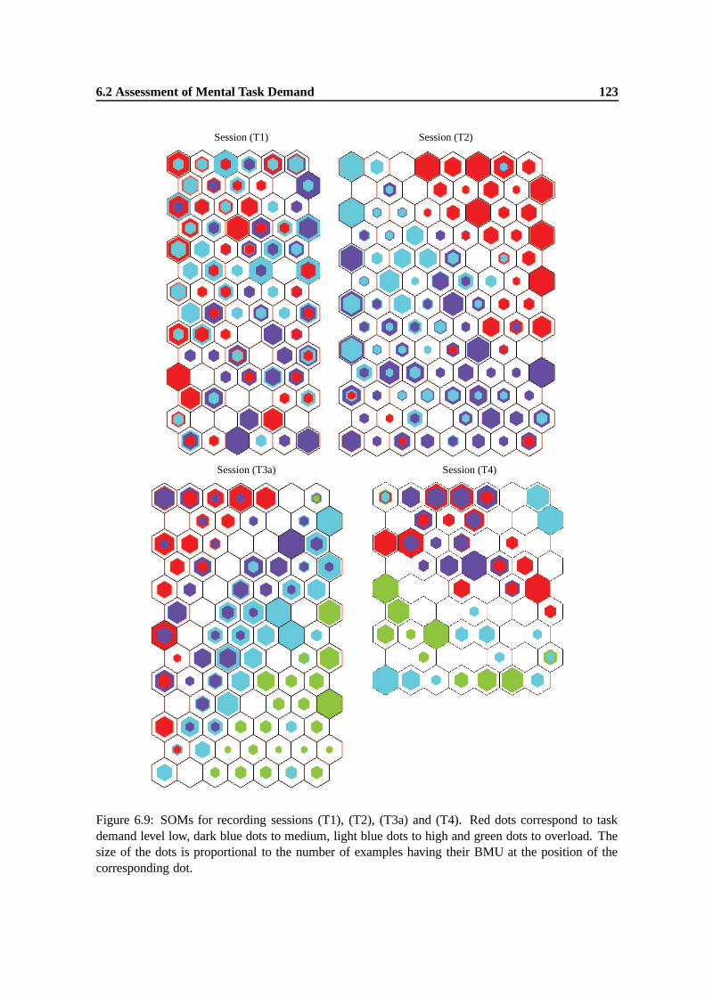
6.2 Assessment of Mental Task Demand 123
Session (T1) Session (T2)
Session (T3a) Session (T4)
Figure 6.9: SOMs for recording sessions (T1), (T2), (T3a) and (T4). Red dots correspond to taskdemand level low, dark blue dots to medium, light blue dots to high and green dots to overload. Thesize of the dots is proportional to the number of examples having their BMU at the position of thecorresponding dot.
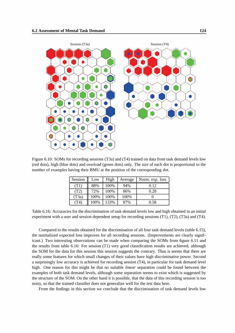
6.2 Assessment of Mental Task Demand 124
Session (T3a) Session (T4)
Figure 6.10: SOMs for recording sessions (T3a) and (T4) trained on data from task demand levels low(red dots), high (blue dots) and overload (green dots) only. The size of each dot is proportional to thenumber of examples having their BMU at the position of the corresponding dot.
Session Low High Average Norm. exp. loss
(T1) 88% 100% 94% 0.12(T2) 72% 100% 86% 0.28(T3a) 100% 100% 100% 0(T4) 100% 133% 87% 0.58
Table 6.16: Accuracies for the discrimination of task demand levels low and high obtained in an initialexperiment with a user and session dependent setup for recording sessions (T1), (T2), (T3a) and (T4).
Compared to the results obtained for the discrimination of all four task demand levels (table 6.15),the normalized expected loss improves for all recording sessions. (Improvements are clearly signif-icant.) Two interesting observations can be made when comparing the SOMs from figure 6.11 andthe results from table 6.16: For session (T1) very good classification results are achieved, althoughthe SOM for the data for this session this session suggests the contrary. Thus is seems that there arereally some features for which small changes of their values have high discriminative power. Seconda surprisingly low accuracy is achieved for recording session (T4), in particular for task demand levelhigh. One reason for this might be that no suitable linear separation could be found between theexamples of both task demand levels, although some separation seems to exist which is suggested bythe structure of the SOM. On the other hand it is possible, that the data of this recording session is toonoisy, so that the trained classifier does not generalize well for the test data here.
From the findings in this section we conclude that the discrimination of task demand levels low
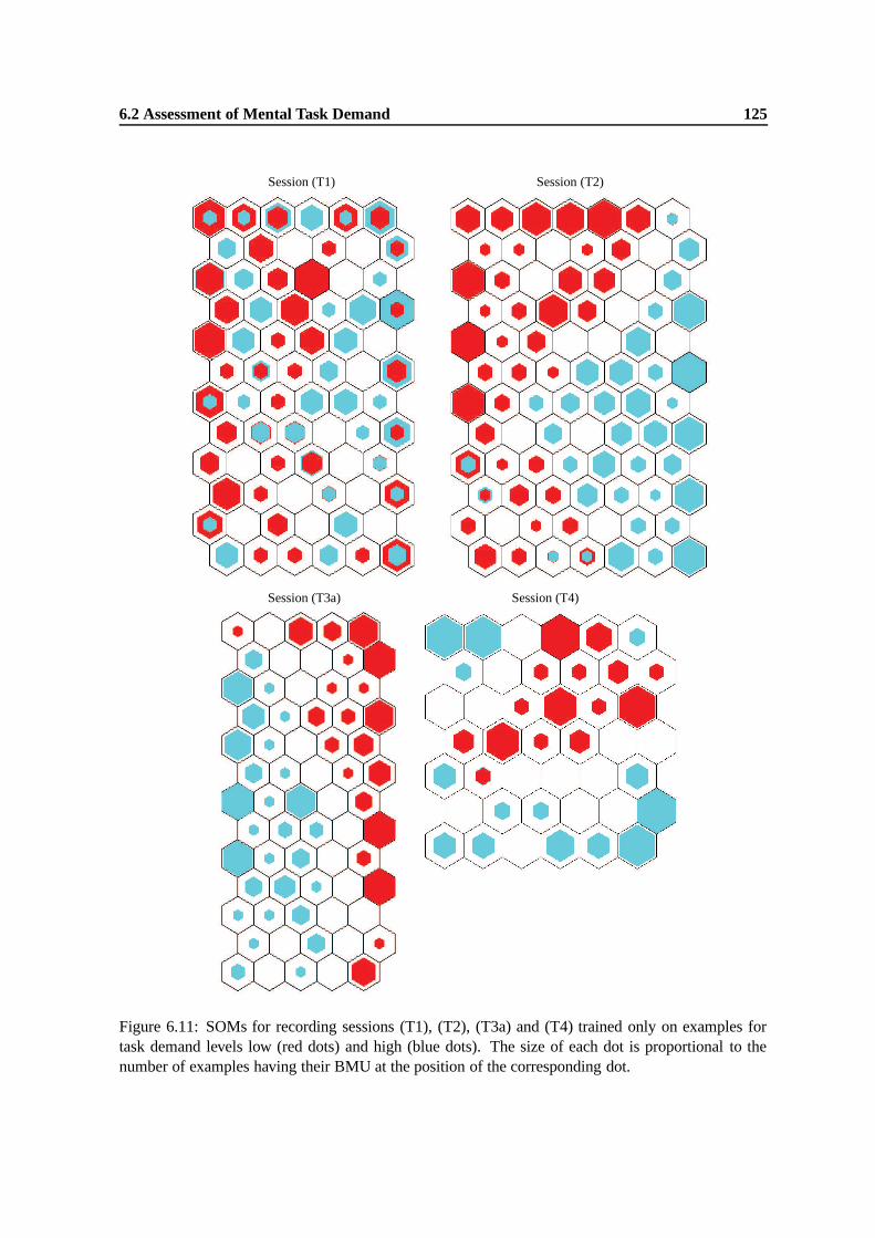
6.2 Assessment of Mental Task Demand 125
Session (T1) Session (T2)
Session (T3a) Session (T4)
Figure 6.11: SOMs for recording sessions (T1), (T2), (T3a) and (T4) trained only on examples fortask demand levels low (red dots) and high (blue dots). The size of each dot is proportional to thenumber of examples having their BMU at the position of the corresponding dot.
6.2 Assessment of Mental Task Demand 126
and high seems to work relatively well. Therefore only these two task demand levels were consideredin the experiments presented in the following sections.
6.2.2 Experimental Setups
The experimental setups for the task demand data are very similar to those which were distinguishedfor the user state data. Therefore the same names for similar setups setups are used here to make iteasier to remember their characteristics. Each setup is now described briefly below:
UD User and session dependent experiments: Different data portions of the same recording sessionwere extracted for training (80% of the whole session), testing and validation (each 10% of thewhole session). Recording sessions (T1), (T2), (T3b) and (T4) from the ElectroCapSubjectsdata collection were used for this setup and results are always reported as averages over thetest or validation set accuracies for all these sessions if not indicated differently. Training setscomprise in average 247 seconds of data, validation sets 31 seconds and test sets 64 seconds.
HB The same type of experiments as for setup UD was conducted on the HeadBandSubjects data(recording sessions (T7) and (T8)). The average size of the training sets is here 314 seconds,the average validation set size 39 seconds and the average test set size 86 seconds. Also herereported results are averages over the accuracies obtained for the validation or test sets of bothrecording sessions.
UI User independent experiments: For recording sessions (T1), (T2), (T3b) and (T4) from the Elec-troCapSubjects data the system was trained in a round-robin manner on a subset of threerecording sessions (in average 740 seconds of data) and tested on the remaining session. Forcomparability of the results the same test sets as in setup UD were used and results were aver-aged in the same way. For validation 229 seconds of data from the sessions (T5) and (T6) fromthe ElectroCapSubjects data collection were available.
SI User dependent but session independent experiments: Only for one subject task demand data wascollected twice (recording sessions (T3a) and (T3b)). For this data, experiments across sessionswere conducted, i.e. training was performed on 80% of the data of one session (in average 257seconds of data), testing on 10% of the other session (in average 48 seconds of data) and viceversa. Results are reported as averages over the accuracies from both test sets. As in case ofthe user state data, no data was available for validation here, which reflects the properties of asession independent experimental setup. For early stopping regularization 10% of non-trainingdata from the training sessions was used (in average 32 seconds). In all other cases plausibleguesses for system parameters were made based on the estimates for setups UD and UI.
Note that also for the task demand data the length of the different data sets in seconds correspondsto the number of feature vectors per data set, since for each second a new feature vector is available,as explained in section 4.2. Note furthermore that data sets for training and validation were balancedafter their extraction from the different recording sessions (as in case of the user state data), so thatthe percentages given above do not represent their fraction of all available data. For the test data thisis not the case, which also explains the difference between the available test and validation data, evenwhen the same amount of data had been extracted for both prior to balancing.
Similarly to the user state data (see section 6.1.1), the test sets for setups UD and UI are exactlythe same, while the test sets for the other two setups are based on different recording sessions. For this

6.2 Assessment of Mental Task Demand 127
reason accuracies obtained for setups UD and UI are clearly separated from the accuracies obtainedfor the other setups in all following tables in the same way as is has been done for the user state data.
6.2.3 ANN topology selection
As explained in section 6.1.2 for the user state data, ANN topology selection had to be performed aswell for the task demand data, before ANNs can be trained and used for task demand prediction. Alsohere exclusively networks with one hidden layer are used so that only the number of neurons in thehidden layer remains to be determined.
For setup UD this is done using the data from recording sessions (T5) and (T6) (the validationdata sessions for setup UI). For setup UI networks are trained on the original training data and earlystopping regularization is performed using the original validation data. As topology section test setdata portions from recording sessions (T5) and (T6) are used which are disjoint with the originalvalidation data. No data is available to perform topology selection for setup SI. Therefore the networktopology for this setup was guessed based on the results obtained for the other two setups.
Figure 6.12 shows the accuracies for different numbers of neurons in the hidden layer obtainedwith regression and classification ANNs for setups UD and UI. Accuracies represent always aver-ages over five repetitions of the same experiment. The standard deviations over these repetitions aredepicted by the whiskers in the figure. From the predictions of regression ANNs accuracies wereobtained using equation 4.71.
Several observations can be made in figure 6.12. For both experimental setups regression ANNsperform slightly better than classification ANNs, however differences in results are in most cases verysmall (except when less than 8 hidden units are used in case of setup UD) and often within the standarddeviations over the repeated experiments. Thus the hypothesis from section 4.5 that different taskdemand levels are predicted better when using a regression function instead of a classification function(since the first method exploits the information contained in the ordinal scaling of the different taskdemand levels) is supported only slightly by that finding. Furthermore closer inspection of the resultsfor particular recording sessions reveals that fluctuations across subjects are larger when a regressionANN instead of a classification ANN is used.
For setup UD the classification results increase when increasing the number of hidden units up to14, while regression results seem to be mostly insensitive towards the number of hidden units. There-fore in the following ANN experiments using setup UD 18 hidden units were used for classificationANNs and 14 hidden units for regression ANNs.
For setup UI it can be seen that results are only slightly above chance accuracy. Therefore ithas to be investigated in the following, whether it is generally possible to predict task demand acrosssubjects, and if this is the case, whether ANNs are applicable for this task. Besides that it can be seenthat results for classification and regression ANNs are insensitive towards the number of hidden units.Therefore 14 hidden units were used for both methods in the following experiments using setup UI.Also for setup SI 14 hidden units were used for all ANN experiments.
6.2.4 Comparison of Prediction Methods
In this section the performance of the regression and classification versions of SVMs and ANNs arecompared for the following baseline system configuration:
• no artifact removal
• no averaging over feature vectors
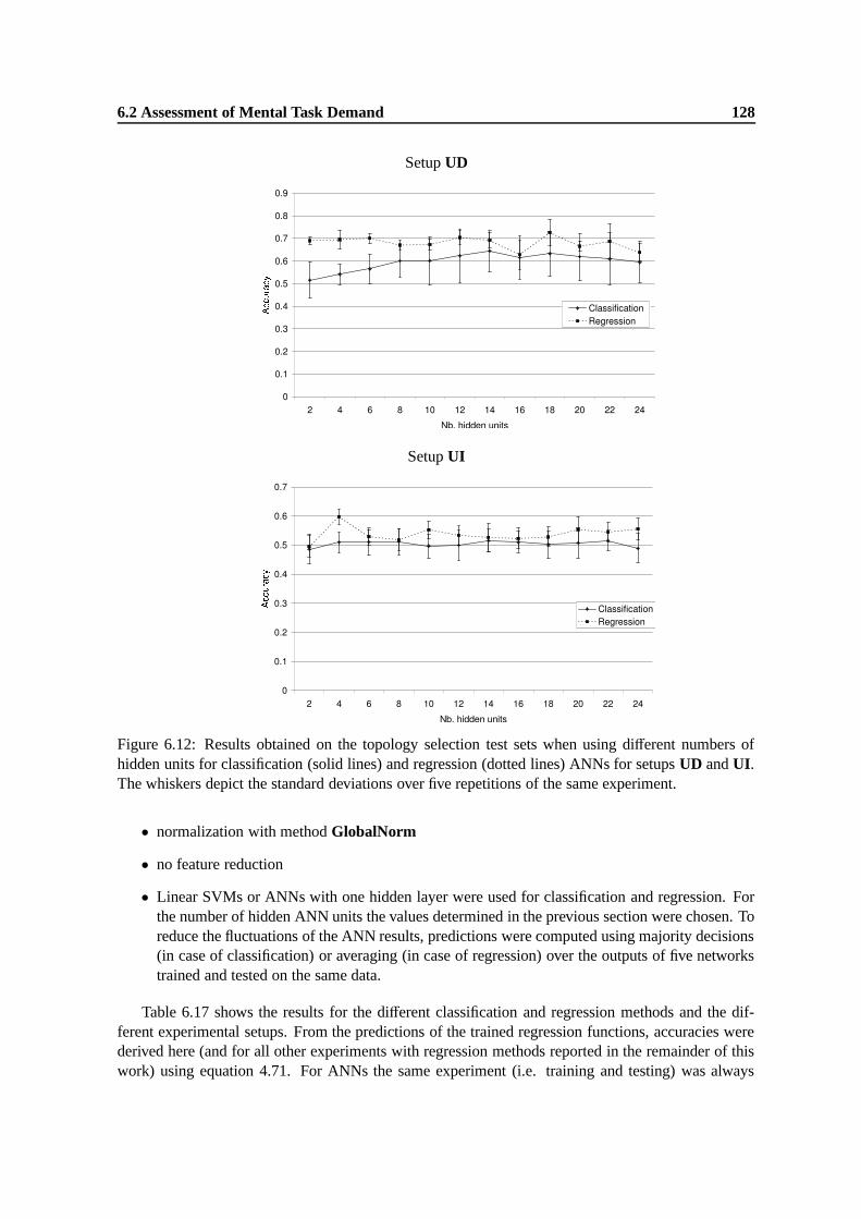
6.2 Assessment of Mental Task Demand 128
Setup UD
Setup UI
Figure 6.12: Results obtained on the topology selection test sets when using different numbers ofhidden units for classification (solid lines) and regression (dotted lines) ANNs for setups UD and UI.The whiskers depict the standard deviations over five repetitions of the same experiment.
• normalization with method GlobalNorm
• no feature reduction
• Linear SVMs or ANNs with one hidden layer were used for classification and regression. Forthe number of hidden ANN units the values determined in the previous section were chosen. Toreduce the fluctuations of the ANN results, predictions were computed using majority decisions(in case of classification) or averaging (in case of regression) over the outputs of five networkstrained and tested on the same data.
Table 6.17 shows the results for the different classification and regression methods and the dif-ferent experimental setups. From the predictions of the trained regression functions, accuracies werederived here (and for all other experiments with regression methods reported in the remainder of thiswork) using equation 4.71. For ANNs the same experiment (i.e. training and testing) was always
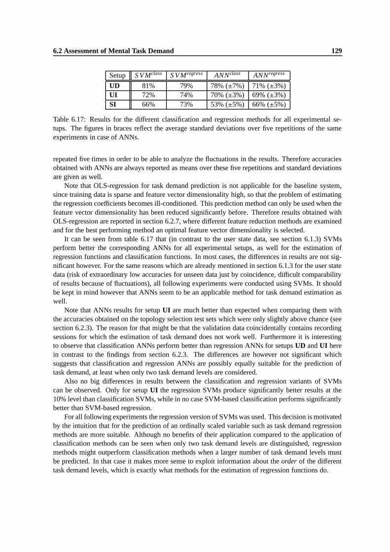
6.2 Assessment of Mental Task Demand 129
Setup S V Mclass S V Mregress ANNclass ANNregress
UD 81% 79% 78% (±7%) 71% (±3%)UI 72% 74% 70% (±3%) 69% (±3%)SI 66% 73% 53% (±5%) 66% (±5%)
Table 6.17: Results for the different classification and regression methods for all experimental se-tups. The figures in braces reflect the average standard deviations over five repetitions of the sameexperiments in case of ANNs.
repeated five times in order to be able to analyze the fluctuations in the results. Therefore accuraciesobtained with ANNs are always reported as means over these five repetitions and standard deviationsare given as well.
Note that OLS-regression for task demand prediction is not applicable for the baseline system,since training data is sparse and feature vector dimensionality high, so that the problem of estimatingthe regression coefficients becomes ill-conditioned. This prediction method can only be used when thefeature vector dimensionality has been reduced significantly before. Therefore results obtained withOLS-regression are reported in section 6.2.7, where different feature reduction methods are examinedand for the best performing method an optimal feature vector dimensionality is selected.
It can be seen from table 6.17 that (in contrast to the user state data, see section 6.1.3) SVMsperform better the corresponding ANNs for all experimental setups, as well for the estimation ofregression functions and classification functions. In most cases, the differences in results are not sig-nificant however. For the same reasons which are already mentioned in section 6.1.3 for the user statedata (risk of extraordinary low accuracies for unseen data just by coincidence, difficult comparabilityof results because of fluctuations), all following experiments were conducted using SVMs. It shouldbe kept in mind however that ANNs seem to be an applicable method for task demand estimation aswell.
Note that ANNs results for setup UI are much better than expected when comparing them withthe accuracies obtained on the topology selection test sets which were only slightly above chance (seesection 6.2.3). The reason for that might be that the validation data coincidentally contains recordingsessions for which the estimation of task demand does not work well. Furthermore it is interestingto observe that classification ANNs perform better than regression ANNs for setups UD and UI herein contrast to the findings from section 6.2.3. The differences are however not significant whichsuggests that classification and regression ANNs are possibly equally suitable for the prediction oftask demand, at least when only two task demand levels are considered.
Also no big differences in results between the classification and regression variants of SVMscan be observed. Only for setup UI the regression SVMs produce significantly better results at the10% level than classification SVMs, while in no case SVM-based classification performs significantlybetter than SVM-based regression.
For all following experiments the regression version of SVMs was used. This decision is motivatedby the intuition that for the prediction of an ordinally scaled variable such as task demand regressionmethods are more suitable. Although no benefits of their application compared to the application ofclassification methods can be seen when only two task demand levels are distinguished, regressionmethods might outperform classification methods when a larger number of task demand levels mustbe predicted. In that case it makes more sense to exploit information about the order of the differenttask demand levels, which is exactly what methods for the estimation of regression functions do.

6.2 Assessment of Mental Task Demand 130
In figure 6.13 the predictions of the learned regression functions are compared with the targetvalues for low task demand (target values 1) and high task demand (target value 2). The classificationaccuracies which can be derived from these predictions are shown in figure 6.14 for each recordingsession and each experimental setup.
The relation between the regression function predictions (figure 6.13) and the classification accu-racies derived from these predictions (figure 6.14) is now discussed separately for each experimentalsetup.
For setup UD it can be seen that the predictions for session (T3a) match the targets very well andthat they show little variability. This results in a classification accuracy of 100% for this session. Forsessions (T1) and (T2) much more variabilty in the predictions can be observed. However predictionswhich belong to examples for high task demand have in average higher values than those beloningto examples for low task demand. The values of the latter are generally much higher than theirtarget values. The effect of both observations on classification accuracies is, that the performance forhigh task demand is much better than the performance for low task demand for both sessions. Allpredictions for the test data of session (T4) are approximately on the same level. It can easily beseen that those belonging to examples of high task demand are much too low in order to produce thecorrect classification. Note however there is a slight tendency of these predictions to be higher thanthe predicted values for examples for low task demand.
For experimental setup UI it is interesting to observe that for sessions (T2) and (T4) better clas-sification accuracies are achieved compared to setup UD. That means that data recorded from othersubjects is better suited to predict the task demand for these two sessions, than data which is takenfrom these sessions themselves. The variability of predictions is large for setup UI, too. In particularfor session (T1) it surprising that classification accuracies clearly above chance are achieved, althoughpredictions seem almost randomly spread between the target values for low and high task demand. Ingeneral results for setup UI are much better than expected according to the experience made for theuser state data (see section 6.1.3).
When comparing the predictions for recording session (T3a) for setups UD and SI, it can be seenthat the predicted values contain much more variability when another recording session from the samesubject is used for training. Nevertheless predictions belonging to examples for low task demand aresufficiently low, and those for high task demand are sufficiently high also for setup SI, so that stillgood classification accuracies are obtained. For session (T3b) a similar observation as for session(T4) in case of setup UD can be made: The predictions for examples for high task demand stay tooclose to the target value for low task demand, so that only the chance classification accuracy of 50%is obtained, since all examples are classified as low task demand.
Table 6.18 finally shows for each recording session and each experimental setup some statisticalmeasures which are suitable for the evaluation of regression functions (see section 4.6.2) together withthe average classification accuracy for comparison.
It can be seen that high values for rub and low values of the squared error do not necessarilyimply good classification accuracies. The main reason for this seems to be, that despite the largevariability of the predictions in many cases, the predicted values are still closer to their target valuethan to the target value of the other task demand level, so that good classification accuracies areobtained. In our case that means that predictions for examples for low or high task demand whichare only slightly below or above 1.5 may lead to good classification accuracies, while they producehigh squared errors and low correlation coefficients. Furthermore it is interesting to observe the (inmost cases) largely positive offsets of the linear regression functions. This shows that task demandpredictions are generally higher than they should be, what can also be seen in figure 6.13, in particularfor the examples for low task demand.
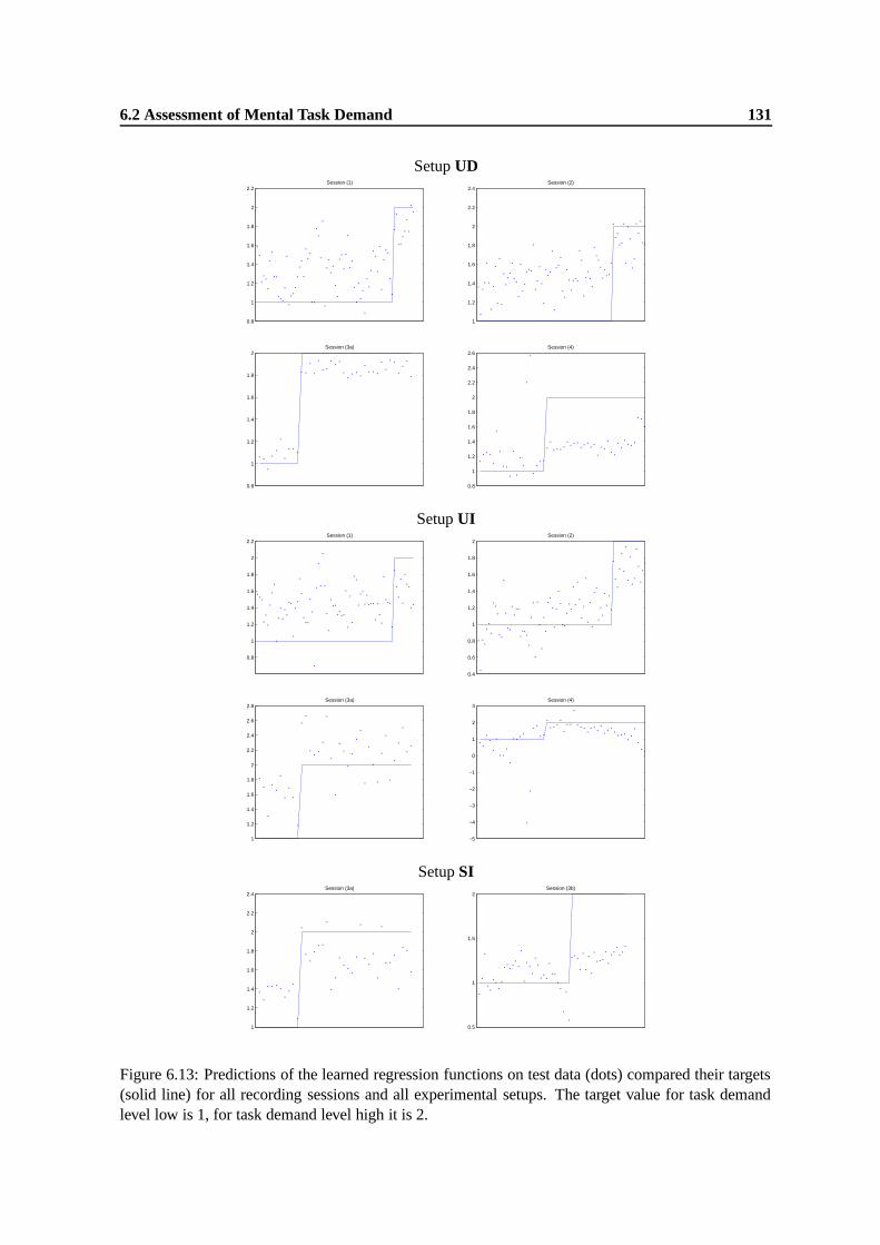
6.2 Assessment of Mental Task Demand 131
Setup UD
0.8
1
1.2
1.4
1.6
1.8
2
2.2Session (1)
1
1.2
1.4
1.6
1.8
2
2.2
2.4Session (2)
0.8
1
1.2
1.4
1.6
1.8
2Session (3a)
0.8
1
1.2
1.4
1.6
1.8
2
2.2
2.4
2.6Session (4)
Setup UI
0.8
1
1.2
1.4
1.6
1.8
2
2.2Session (1)
0.4
0.6
0.8
1
1.2
1.4
1.6
1.8
2Session (2)
1
1.2
1.4
1.6
1.8
2
2.2
2.4
2.6
2.8Session (3a)
−5
−4
−3
−2
−1
0
1
2
3Session (4)
Setup SI
1
1.2
1.4
1.6
1.8
2
2.2
2.4Session (3a)
0.5
1
1.5
2Session (3b)
Figure 6.13: Predictions of the learned regression functions on test data (dots) compared their targets(solid line) for all recording sessions and all experimental setups. The target value for task demandlevel low is 1, for task demand level high it is 2.
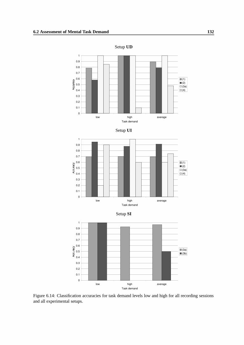
6.2 Assessment of Mental Task Demand 132
Setup UD
Setup UI
Setup SI
Figure 6.14: Classification accuracies for task demand levels low and high for all recording sessionsand all experimental setups.

6.2 Assessment of Mental Task Demand 133
Setup UDSession rub S Eub reg. fctn av. accuracy
(T1) 0.62 0.32 t = 0.48p + 0.83 89%(T2) 0.68 0.37 t = 0.40p + 1.06 79%(T3a) 0.98 0.13 t = 0.77p + 0.32 100%(T4) 0.24 0.56 t = 0.10p + 1.16 48%
Setup UISession rub S Eub reg. fctn av. accuracy
(T1) 0.43 0.44 t = 0.20p + 1.23 70%(T2) 0.70 0.31 t = 0.57p + 0.53 91%(T3a) 0.71 0.51 t = 0.59p + 1.02 60%(T4) 0.55 1.12 t = 1.07p − 0.62 75%
Setup SISession rub S Eub reg. fctn av. accuracy
(T3a) 0.71 0.35 t = 0.38p + 0.98 96%(T3b) 0.65 0.53 t = 0.21p + 0.86 50%
Table 6.18: Correlation coefficient rub and squared error (S Eub) for unbalanced data sets and linear re-gression functions between targets (t) and predictions (p)obtained for the different recording sessionsand different experimental setups. In the last column the average classification accuracies are shownfor comparison.
We conclude that for all experimental setups SVM-based regression function estimation for taskdemand prediction works comparatively well, although single recording sessions exist where no morethan chance accuracy is achieved (session (T4) for setup UD and session (T3b) for setup SI). Thisindicates that there are data sets for which task demand can not be predicted well with our methods,at least for the baseline system configuration. Next it is important to remark that in many cases wheregood classification accuracies are achieved, the variability of the predicted values is nevertheless largeand predictions often do not match their targets very well, what can be seen from figure 6.13. Thestatistical measures characterizing the estimated regression functions confirm that finding. This showsthat in many cases predictions of class labels are not very stable and that the problem of task demandestimation, even when it is reduced to the problem of distinguishing two task demand levels, stillremains difficult.
Although it is important to keep in mind that classification accuracies are always derived frompredictions of regression functions here, experimental results are reported mostly in terms of accura-cies in the following. We believe that this measure provides the best overview over changes of thesystem performance when different parameters are varied.
6.2.5 Averaging
Also for the task demand data the effect of averaging over the k previous feature vectors was examined.Figure 6.15 shows the validation set accuracies for setups UD and UI for different values of k.
Compared to the user state data (see figure 6.4), improvements achieved by averaging are relativelysmall. For setup UI the best results are observed for k = 2 in contrast to the expectation that results
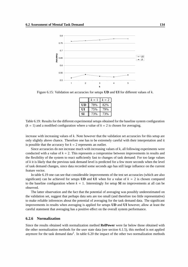
6.2 Assessment of Mental Task Demand 134
Figure 6.15: Validation set accuracies for setups UD and UI for different values of k.
k = 1 k = 2
UD 78% 82%UI 75% 79%SI 73% 73%
Table 6.19: Results for the different experimental setups obtained for the baseline system configuration(k = 1) and a modified configuration where a value of k = 2 is chosen for averaging.
increase with increasing values of k. Note however that the validation set accuracies for this setup areonly slightly above chance. Therefore one has to be extremely careful with their interpretation and itis possible that the accuracy for k = 2 represents an outlier.
Since accuracies do not increase much with increasing values of k, all following experiments wereconducted with a value of k = 2. This represents a compromise between improvements in results andthe flexibility of the system to react sufficiently fast to changes of task demand: For too large valuesof k it is likely that the previous task demand level is predicted for a few more seconds when the levelof task demand changes, since data recorded some seconds ago has still large influence on the currentfeature vector.
In table 6.19 one can see that considerable improvements of the test set accuracies (which are alsosignificant) can be achieved for setups UD and UI when for a value of k = 2 is chosen comparedto the baseline configuration where k = 1. Interestingly for setup SI no improvements at all can beobserved.
The latter observation and the fact that the potential of averaging was possibly underestimated onthe validation set, suggest that perhaps data sets are too small (and therefore too little representative)to make reliable inferences about the potential of averaging for the task demand data. The significantimprovements in results when averaging is applied for setups UD and UI however, allow at least thecareful statement that averaging has a positive effect on the overall system performance.
6.2.6 Normalization
Since the results obtained with normalization method RelPower were far below those obtained withthe other normalization methods for the user state data (see section 6.1.5), this method is not appliedanymore for the task demand data2. In table 6.20 the impact of the other two normalization methods
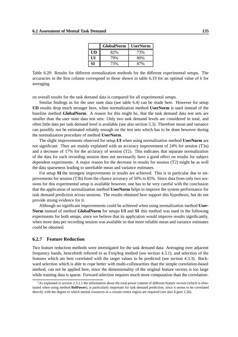
6.2 Assessment of Mental Task Demand 135
GlobalNorm UserNorm
UD 82% 73%UI 79% 80%SI 73% 87%
Table 6.20: Results for different normalization methods for the different experimental setups. Theaccuracies in the first column correspond to those shown in table 6.19 for an optimal value of k foraveraging.
on overall results for the task demand data is compared for all experimental setups.Similar findings as for the user state data (see table 6.4) can be made here. However for setup
UD results drop much stronger here, when normalization method UserNorm is used instead of thebaseline method GlobalNorm. A reason for this might be, that the task demand data test sets aresmaller than the user state data test sets: Only two task demand levels are considered in total, andoften little data per task demand level is available (see also section 5.3). Therefore mean and variancecan possibly not be estimated reliably enough on the test sets which has to be done however duringthe normalization procedure of method UserNorm.
The slight improvements observed for setup UI when using normalization method UserNorm arenot significant. They are mainly explained with an accuracy improvement of 24% for session (T3a)and a decrease of 17% for the accuracy of session (T2). This indicates that separate normalizationof the data for each recording session does not necessarily have a good effect on results for subjectdependent experiments. A major reason for the decrease in results for session (T2) might be as wellthe data sparseness leading to unreliable mean and variance estimates.
For setup SI the strongest improvements in results are achieved. This is in particular due to im-provements for session (T3b) from the chance accuracy of 50% to 85%. Since data from only two ses-sions for this experimental setup is available however, one has to be very careful with the conclusionthat the application of normalization method UserNorm helps to improve the system performance fortask demand prediction across sessions. The results obtained here support this hypothesis, but do notprovide strong evidence for it.
Although no significant improvements could be achieved when using normalization method User-Norm instead of method GlobalNorm for setups UI and SI this method was used in the followingexperiments for both setups, since we believe that its application would improve results significantly,when more data per recording session was available so that more reliable mean and variance estimatescould be obtained.
6.2.7 Feature Reduction
Two feature reduction methods were investigated for the task demand data: Averaging over adjacentfrequency bands, henceforth referred to as FreqAvg method (see section 4.3.1), and selection of thefeatures which are best correlated with the target values to be predicted (see section 4.3.3). Back-ward selection which is able to cope better with multi-collinearities than the simple correlation-basedmethod, can not be applied here, since the dimensionality of the original feature vectors is too largewhile training data is sparse. Forward selection requires much more computation than the correlation-
2As explained in section 2.3.2.1 the information about the total power content of different feature vectors (which is elim-inated when using method RelPower), is particularly important for task demand prediction, since it seems to be correlateddirectly with the degree to which mental resources in a certain cortex region are required (see also figure 2.26).

6.2 Assessment of Mental Task Demand 136
Figure 6.16: Validation set accuracies for setups UD and UI when different bin sizes for the FreqAvgmethod are used. The optimal system configuration for averaging and normalization (as determinedin the previous sections) was used for both setups.
based approach, but it can not be shown that is better able to avoid the problem of multi-collinearities(see section 4.3.3). Therefore it is not applied here as well.
Figure 6.16 shows validation set accuracies when averaging over a different number of adjacentfrequency bands is performed, i.e. when adjacent frequency bands are put into bins of different sizes b,for setups UD and UI. A very similar tendency as already observed for the user state data (see section6.2.7) can be seen here: Accuracies fluctuate in a comparatively small range for all bin sizes between 1and 45 and they decrease strongly only for a bin size of 90. We conclude that also for the task demanddata the information about the power content of lower and upper frequencies per electrode as a wholeseems to be sufficient to obtain acceptable predictions. Note that here again validation set results forsetup UI are only slightly above chance. Therefore one must be careful with their interpretation.
Figure 6.17 shows validation set results for the correlation-based feature reduction method forsetups UD and UI. For setup UD results for feature vector dimensionalities below 100 are much betterthan those obtained with higher feature vector dimensionalities or even without feature reduction, andthey do not drop even when the number of features is reduced down to 16. Only 16 features, i.e. onefeature per electrode, are also used for a bin size of 90 for the FreqAvg method. Here results dropstrongly compared to larger feature vector sizes which can be seen from figure 6.16.
For setup UI no large changes in results can be observed when reducing the feature vector di-mensionality with the correlation-based method. However, also for this setup results do not decreasewhen using only 16 features are used, compared to the case where the feature vector dimensionality isreduced to 16 with the FreqAvg method. A reason that the correlation-based method can not improveresults for this setup could be (besides the problem of validation set accuracies close to chance), thatfor different subjects different features have the largest predictive power (see also table 6.22 below).Therefore the features selected by the correlation based method are not necessarily highly correlatedwith the targets for the test data, but with the targets of data from different subjects in the training set.
We conclude that the correlation-based feature reduction method seems more suitable for featurereduction than the FreqAvg method for the problem of task demand prediction. Note that on the taskdemand data for setup UD even improvements of results could be achieved when correlation-basedfeature reduction was performed, in contrast to the user state data, where for the application of bothLDA (to setup UI) and the FreqAvg method (to both setups) results could only be kept constantly

6.2 Assessment of Mental Task Demand 137
Figure 6.17: Validation set accuracies for correlation-based feature reduction to different feature vec-tor dimensionalities for setups UD and setup UI. The optimal system configuration for averaging andnormalization (as determined in the previous sections) was used for both setups.
Figure 6.18: Development of the standard deviation over the validation set accuracies obtained fordifferent recording sessions for setup UD when the number of features is reduced with the correlation-based method.
when reducing the feature vector dimensionality. That shows that for session dependent estimation oftask demand linear feature reduction methods are suitable.
For setup UD it is interesting to observe the relation between the standard deviation over the resultsfrom different recording sessions and the feature vector dimensionality when correlation-based featurereduction is performed (see figure 6.18): For a smaller number of features the standard deviationbecomes smaller as well. Accuracies which are already high for a larger feature vector dimensionalitydecrease a little (sessions (T1) and (T3a)), while previously low accuracies increase considerably(sessions (T2) and (T4)) for a reduced number of features. This indicates that feature reduction is inparticular useful when for a high number of features accuracies are low. In that case, the correlation-based feature reduction method seems to be able to sort out features which introduce a lot of noise inthe data (apparently more than SVMs could cope with) and whose presence in the feature vectors istherefore harmful to the predictions.

6.2 Assessment of Mental Task Demand 138
No feature reduction Corr.-based feat. reduc-tion
UD 82% 92% (80 features)UI 80% 77% (240 features)SI 87% 61% (240 features)
Table 6.21: Results obtained for feature reduction with the correlation-based method for the differentexperimental setups compared to the results obtained without feature reduction. In braces the numberof used features for each setup is given. Results for the particular setups are always achieved withtheir optimal system configuration for averaging and normalization.
Table 6.21 compares finally the test set results obtained without feature reduction to those obtainedusing correlation-based feature reduction method. Based on the validation set results from figure 6.17a feature vector dimensionality of 80 was determined for setup UD. For setup UI we argued abovethat the features selected on the training data are not necessarily the best correlated features with thetarget values of the test data. Therefore we decided to allow a three times larger feature vector size of240 for this setup to increase the chance that also features with high predictive power for the test dataare included. This feature vector size was also chosen for setup SI.
While accuracies for setup UD increase by 10%, a decrease of results for the other setups canbe observed, although a larger feature vector size was allowed here. The most likely reason for thatis that features with the largest predictive power for the test sets are still not included in the featurevectors. This shows that features which are suitable for the prediction of task demand seem to differ alot across subjects and even across sessions.
For setup UD where correlation-based feature reduction yields improvements in results, it is inter-esting to analyze which features are selected for the different recording sessions, i.e. for the differentsubjects. In table 6.22 for each session the number of features selected per electrode channel isshown. No commonalities for all recording sessions can be found, however some similarities betweentwo pairs of sessions are noteworthy. For recording sessions (T1) and (T2) electrode T4 has a largeimportance, although the pre-frontal electrodes Fp1 and Fp2 play an even more important role in caseof recording session (T1). For session (T2) only for electrode Fp2 some more features than for otherelectrodes are selected, but the largest number of features is still taken from electrode T4. Record-ing sessions (T3a) and (T4) share the importance of electrode O1. While for session (T3a) the datafrom O1 only is sufficient to make good predictions however, for session (T4) also the frontal and thefronto-temporal cortex plays an important role.
We conclude that features which are most correlated with task demand are generally subject-specific, although there are remarkable similarities at least between groups of subjects. On the otherhand one finds for setup SI that there are little similarities between the features selected for the twosessions recorded from the same subject ((T3a) and (T3b)). While for (T3a) all 80 features are chosenfrom electrode O1 as shown above, the fronto-temporal cortex and the parietal cortex are preferredfor session (T3b). Therefore it seems that the selected features are not (or not only) subject-specific,but possibly also task-specific. This becomes clear when considering that different types of men-tal resources are required when different presentations are given to one subject. While during onepresentation mathematical reasoning might be more important, for another one the understanding ofsketches and visual perception could be required. Naturally, in both cases the correlates of differenttask demand levels are observed most pronounced at different cortex regions as explained in section2.3.

6.2 Assessment of Mental Task Demand 139
Session Fp1 Fp2 F7 F8 F3 F4 Fz T3 T4 T5 T6 P3 P4 Pz O1 O2
(T1) 36 13 3 0 3 0 1 1 12 0 6 1 1 3 0 0(T2) 2 9 0 2 1 0 2 2 59 3 0 0 0 0 0 0(T3a) 0 0 0 0 0 0 0 0 0 0 0 0 0 0 80 0(T4) 0 6 4 8 5 4 5 5 6 1 3 1 5 3 21 3
Table 6.22: Number of features selected per electrode for the different recording sessions of setupUD, when correlation based reduction to 80 features is performed.
S V Mregress OLS-Regression
UD 92% 79%UI 77% 77%SI 61% 70%
Table 6.23: Comparison of results achieved by regression SVMs and OLS-regression for the differentexperimental setups. For all setups the feature vector dimensionality is reduced with the correlation-based method to the values shown in table 6.17 for this method.
The analysis of the selected frequency bands for feature reduction to 80 features for the record-ing sessions of setup UD reveals, that mostly frequency bands above 20Hz are preferred, except forsession (T3a) where almost all frequency bands from electrode O1 are chosen. This agrees with thehypothesis from section 2.3.2.1 that in particular high frequent EEG activity is a good correlate oftask demand.
For a comparatively small feature vector dimensionality it becomes finally possible to examinethe performance of OLS-regression for the prediction of task demand. Table 6.23 compares the re-sults obtained with regression SVMs to those obtained using OLS-regression for a feature vectordimensionality of 80. Interestingly only the results for setup UD seem to confirm the hypothesis fromsection 4.5.3 that regression SVMs perform better than OLS-regression, since the latter method doesnot perform any regularization to minimize the acual error instead of the training set error. For setupSI the application of OLS-regression improves results even by 10%. The reason for this is the averageaccuracy obtained with a regression SVM for session (T3b) of 26% (which is far below chance) isincreased to 79% using OLS-regression. Much deeper analysis of the data from sessions (T3a) and(T3b) would probably be required to understand the differences in results obtained with both methods.
6.2.8 Combination of Two Subjective Task Demand Evaluations
In section 5.3 it was mentioned that some subjects evaluated the task demand they experienced duringthe perception of the presentation twice. These two evaluations were then used to create the three datapartitionings Eval1, Eval2 and EvalCombined. In this section the results from experiments with allthree data partitionings are reported and discussed in order to analyze the following issues:
1. Is system performance better for partitioning Eval1 or Eval2? With this question, we want tofind out whether subjects are still able to estimate their task demand while they were given thepresentation some days or even weeks after the actual presentation.
2. Do results improve when using partitioning EvalCombined? Here we want to examine whetherin the data from partitioning EvalCombined (which contains the overlapping time segmentsfrom both evaluations) only those time segments are included for which differences in task

6.2 Assessment of Mental Task Demand 140
Session Eval1 Eval2 EvalCombined
(T2) 88% 78% 72%(T3b) 48% 57% 57%(T4) 98% 91% 90%(T6) 55% 92% 70%Mean 72% 79% 72%
Table 6.24: Average accuracies for the different recording sessions and means over all sessions for datapartitionings Eval1, Eval2 and EvalCombined. Results were obtained using experimental setup UDfor which the optimal parameters for averaging, normalization and feature reduction (as determinedin the previous sections) were chosen.
demand are particularly pronounced, since time segments for which subjects were unsure howto evaluate them are probably removed in this partitioning.
Table 6.24 shows the average accuracies for the different recording sessions (for sessions (T2),(T3b), (T4) and (T6) two task demand evaluations are available) and the mean over all sessions forpartitionings Eval1, Eval2 and EvalCombined. Results are obtained using experimental setup UD.One can see that in average better results are achieved for partitioning Eval1 compared to partition-ing Eval2. In particular the results for sessions (T3b) and (T6) which are below or close to chanceaccuracy for partitioning Eval1 improve when using partitioning Eval2, while results for sessions(T2) and (T4) drop. The difference of the mean accuracies over all recording sessions between bothpartitionings is not significant.
We conclude that even some weeks after the actual perception of the presentation subjects werestill able to give estimates of their task demand during the initial perception of the presentation whichare correlated with their EEG. This seems surprising when the poor overlap between both evaluations(see table 5.4) is considered. On the other hand it must be taken into account however that betweenboth evaluations mostly high task demand and overload or low task demand and medium task demandwere confused (see figure 5.7) and that medium task demand and overload are not considered herefor prediction. Thus the time segments belonging to task demand levels low and high for whichpredictions are made, virtually do not overlap between both partitionings, so that it becomes plausibleagain that acceptable results are obtained for both partitionings.
For the partitioning EvalCombined better results were expected because of the above explainedhypothesis. However it is important to note that the amount of available data decreases when com-bining both evaluations (see also 5.4) which might explain that results do not improve compared topartitioning Eval1 or Eval2. Nevertheless accuracies for all sessions are better compared to thoseobtained when using partitioning Eval1.
6.2.9 Electrode Reduction
Also for the task demand data experiments with a reduced set of electrodes were conducted. Table6.25 compares results obtained for setup UD with those obtained for setups HB and UD4, where datais taken only from the four pre-frontal and frontal electrodes which are also used for the headbandrecordings. When the data from four electrodes only was used for prediction, the application offeature reduction could not improve results. Therefore also for setup UD the results obtained withoutfeature reduction are displayed in table 6.25 for better comparability.

6.2 Assessment of Mental Task Demand 141
Setup UD
Session
(T1) 93%(T2) 79%(T3a) 100%(T4) 57%Mean 82%
Setup UD4
Session
(T1) 91%(T2) 48%(T3a) 86%(T4) 50%Mean 69%
Setup HB
Session
(T7) 89%(T8) 49%Mean 69%
Table 6.25: Accuracies for the different recording sessions and means over all sessions for setupsHB, UDand UD4. In all cases the system is configured optimally according to the findings from theprevious sections. Only feature reduction is not performed.
Setup
Averaging(value ofkopt)
Normalizationmethod
FeatureReduction
UD kopt = 2 GlobalNorm correlation-basedfeature re-duction to80 features
UI kopt = 2 UserNorm noneSI kopt = 2 UserNorm none
Table 6.26: Parameters of the best system configuration for setups UD, SI and UI.
As expected, accuracies drop when using only four pre-frontal and frontal electrodes instead of all16, however they are still clearly above chance. Furthermore there are large fluctuations between theresults for different recording sessions for setups HB and UD4For both setups for half of the sessionsresults are in the same range as for setup UD, while for the rest accuracies are not better than chance.The reason for these fluctuations is possibly the same as above where it was attempted to explain thatacross subjects and sessions different features are selected (section 6.2.7): Only for a certain groupof subjects or a certain type task to be executed, the mental resources required primarily during taskexecution produce an EEG which can be measured using no more than four pre-frontal and frontalelectrodes.
6.2.10 Analysis of Best System Configuration
In this section the best system configuration for each experimental setup is summarized. In table 6.26for all processing steps and all experimental setups the parameters are displayed which lead for eachprocessing step to the largest performance gain. Table 6.27 shows the improvements in results foreach processing step when the optimal parameters for this step are chosen. All results are achievedwith the regression version of a linear SVM.
Note that artifact removal is not considered in tables 6.26 and 6.27, since neither visual inspectionbased nor cross-validation based rejection of independent components could improve results for thetask demand data. Besides the above mentioned problem that ICA weight matrices generalize badly
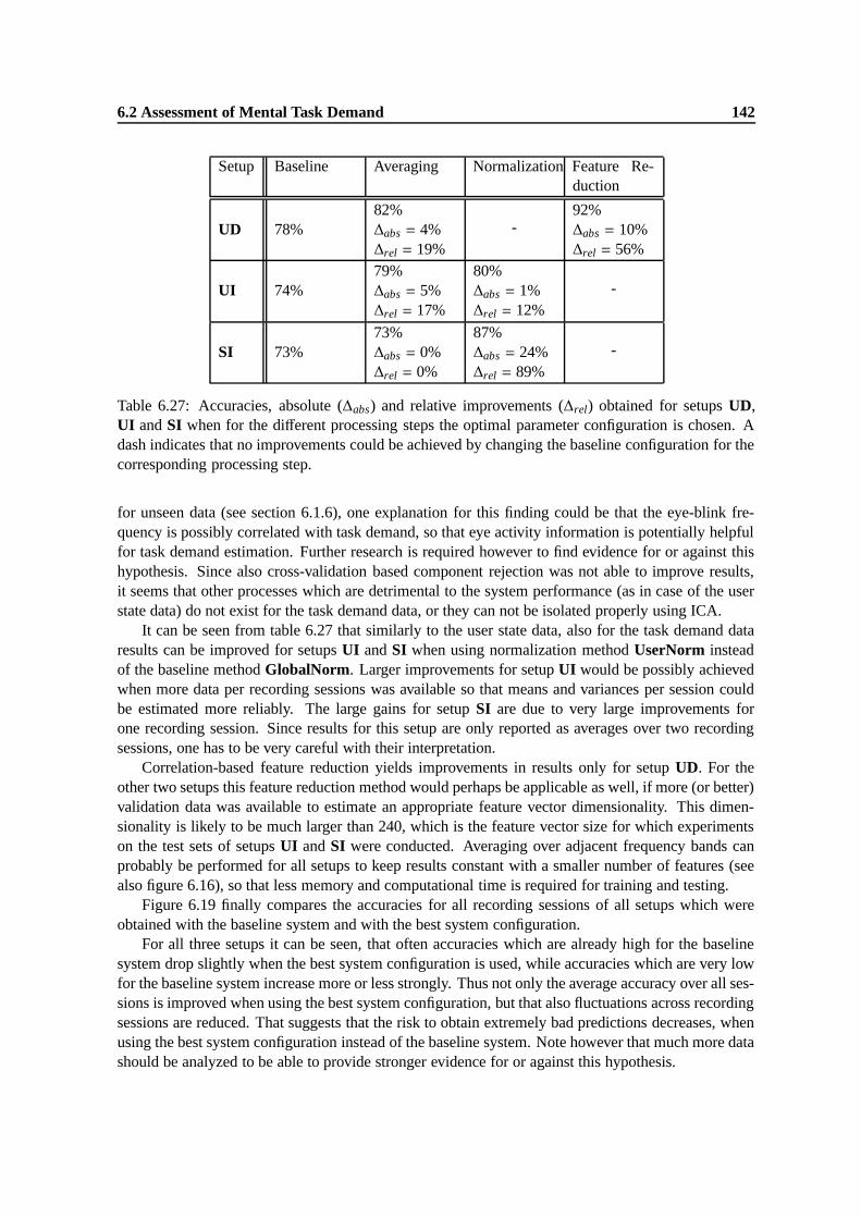
6.2 Assessment of Mental Task Demand 142
Setup Baseline Averaging Normalization Feature Re-duction
UD 78%82%∆abs = 4%∆rel = 19%
-92%∆abs = 10%∆rel = 56%
UI 74%79%∆abs = 5%∆rel = 17%
80%∆abs = 1%∆rel = 12%
-
SI 73%73%∆abs = 0%∆rel = 0%
87%∆abs = 24%∆rel = 89%
-
Table 6.27: Accuracies, absolute (∆abs) and relative improvements (∆rel) obtained for setups UD,UI and SI when for the different processing steps the optimal parameter configuration is chosen. Adash indicates that no improvements could be achieved by changing the baseline configuration for thecorresponding processing step.
for unseen data (see section 6.1.6), one explanation for this finding could be that the eye-blink fre-quency is possibly correlated with task demand, so that eye activity information is potentially helpfulfor task demand estimation. Further research is required however to find evidence for or against thishypothesis. Since also cross-validation based component rejection was not able to improve results,it seems that other processes which are detrimental to the system performance (as in case of the userstate data) do not exist for the task demand data, or they can not be isolated properly using ICA.
It can be seen from table 6.27 that similarly to the user state data, also for the task demand dataresults can be improved for setups UI and SI when using normalization method UserNorm insteadof the baseline method GlobalNorm. Larger improvements for setup UI would be possibly achievedwhen more data per recording sessions was available so that means and variances per session couldbe estimated more reliably. The large gains for setup SI are due to very large improvements forone recording session. Since results for this setup are only reported as averages over two recordingsessions, one has to be very careful with their interpretation.
Correlation-based feature reduction yields improvements in results only for setup UD. For theother two setups this feature reduction method would perhaps be applicable as well, if more (or better)validation data was available to estimate an appropriate feature vector dimensionality. This dimen-sionality is likely to be much larger than 240, which is the feature vector size for which experimentson the test sets of setups UI and SI were conducted. Averaging over adjacent frequency bands canprobably be performed for all setups to keep results constant with a smaller number of features (seealso figure 6.16), so that less memory and computational time is required for training and testing.
Figure 6.19 finally compares the accuracies for all recording sessions of all setups which wereobtained with the baseline system and with the best system configuration.
For all three setups it can be seen, that often accuracies which are already high for the baselinesystem drop slightly when the best system configuration is used, while accuracies which are very lowfor the baseline system increase more or less strongly. Thus not only the average accuracy over all ses-sions is improved when using the best system configuration, but that also fluctuations across recordingsessions are reduced. That suggests that the risk to obtain extremely bad predictions decreases, whenusing the best system configuration instead of the baseline system. Note however that much more datashould be analyzed to be able to provide stronger evidence for or against this hypothesis.
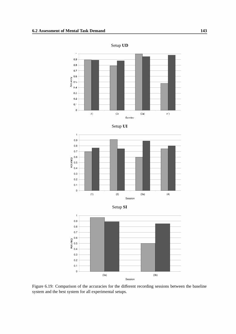
6.2 Assessment of Mental Task Demand 143
Setup UD
Setup UI
Setup SI
Figure 6.19: Comparison of the accuracies for the different recording sessions between the baselinesystem and the best system for all experimental setups.

Chapter 7
Conclusions and Future Work
In this thesis a system for the identification of user states and the assessment of mental task demand us-ing electroencephalographic data has been proposed. For the discrimination of the user states resting,listening, perceiving a presentation, reading an article in a magazine, summarizing the read article andperforming arithmetic operations, classification accuracies of 94.9% in session and subject dependentexperiments, 58.9% in subject independent experiments and 62.7% in subject dependent but sessionindependent experiments could be obtained. For the prediction of low and high task demand duringthe perception of a presentation accuracies of 92.2% in session and subject dependent experiements,80.0% in subject independent experiments and 87.1% in subject dependent but session independentexperiments were achieved.
Potential fields of application for the proposed system are meeting, lecture or office scenarios,where interaction between users and mobile communication devices or face-to-face communicationbetween persons can be improved, when information about user state and task demand is available(see section 1.2). In section 1.1 several goals were formulated which must be fulfilled to make EEGrecording and EEG data processing practical for the mentioned fields of applications. Below it issummarized in how far each of these goals could be met by the research work described in this thesis:
• Robustness: For subject and session dependent experiments accuracies obtained for user stateidentification and task demand estimation are both above 90%. Since these results were achievedwhen no attempt was made to remove artifacts from the data, which usually occur very fre-quently when recording EEG under non-clinical conditions, it seems that artifacts have nostrong negative influence on the overall system performance. ICA-based artifact removal wasonly partially successful. While the rejection of those components containing eye activity couldnot improve results, small but significant improvements were achieved when cross-validationwas applied to identify those components which are most detrimental to classification accura-cies. A general problem of the ICA algorithm used here seemed to be that weights learned ontraining data do not generalize well for unseen data. Besides that the robustness of the systemtowards the variability across sessions and subjects must be increased, since results achieved insession or subject independent experiments are far below those obtained for session and subjectdependent experiments (at least for the user state data).
• Acceptability: In experiments with the headband for EEG recording (see section 5.1 for moredetails about this recording device) it was shown that user state identification and task demandassessment is possible with four electrodes over the pre-frontal and frontal cortex only. Theseare suitable electrode positions for EEG recording in meeting, lecture or office scenarios, since

145
electrodes are easy to attach, no conductive paste gets in contact with the user’s hair and thedata recorded from these electrodes is sufficient to obtain acceptable user state and task demandpredictions in many cases. In the future better positions for electrode attachment should beinvestigated. For instance they could be mounted on a glasses frame or attached behind the earlobes. Thus more cortex regions would be covered compared to the headband which recordssignals from pre-frontal and frontal cortex regions only. Furthermore electrodes at these posi-tions are less visible which might increase the user’s readiness to wear them.
• Real Time Behavior: On a 800 MHz Pentium-3 laptop preprocessing of raw EEG data andprediction of user states takes about one second for more than 100 examples (which correspondsto 100 seconds of data) and much less than one second for five examples using a MATLABTM-based implementation of all algorithms1 . The prediction of task demand requires even lesstime. With the prototype system (see section 6.1.10) it has been demonstrated that user stateprediction is possible in real time.
• Realistic Scenarios: The scenarios used for the data collection and for the experiments withthe prototype system are very different from the highly controlled recording conditions whichmust be fulfilled for clinical EEG recording. On the other hand the proposed system has notbeen tested yet in a real meeting or lecture or during realistic office work. This is however avery essential step which should be made soon. Furthermore the users’ real needs during thescenarios we are aiming at should be investigated more, and it should be examined whetherEEG recording during such scenarios is acceptable for users in general.
We conclude that all formulated goals haven been realized at least partly during the researchdescribed in this thesis, which we consider to be completely satisfactory, since no previous attempttowards EEG-based identification of user states and assessment of task demand in meeting, lecture oroffice scenarios has been made. Besides the above mentioned tasks to be accomplished, there remainalso some other issues to be considered in future research:
• Much more data should be collected, in particular task demand data, to be able to make more re-liable inferences about the system behavior when optimizing its parameters. Also other record-ing setups should be tested (i.e. other user states or other tasks which evoke different taskdemand levels) in order to learn more about the potential and the limits of the proposed meth-ods.
• A deeper insight into the bio-medical background of the EEG would be of advantage to beable to incorporate more a priori knowledge into the system. It should be analyzed for in-stance which are the most meaningful features to be extracted. This does not necessarily haveto be the frequency content of the signals which can be obtained using a Fourier transform.Frequency-based signal representations using wavelets or features which are extracted from thetime signal (in the simplest case the time signal itself and/or its ’derivative’, i.e. its slope) couldbe investigated for example.
• For many processing steps the application of more sophisticated methods should be examined.This includes the use of more robust methods to estimate the frequency spectrum of the signals,
1In the MATLABTM implementation ANNs are used for classification, since no suitable SVM implementation forMATLABTM was available. The S V Mlight software [Joachims, 1999] which was used for SVM-based classification andregression usually requires about 1/100th of a second to make predictions for a few hundred examples of user state or taskdemand data, when the learned model is already in memory.

146
e.g. autoregressive models, the investigation of feature selection techniques which do not implya linear structure of the data and finally the application of non-linear SVMs.
At the end of this work it shall be pointed out that we believe in the large potential of EEGto obtain information about user state and task demand. Such information is extremely useful forthe construction of attentive user interfaces which adapt themselves to the wishes and needs of theirowners. Furthermore inferences about how people interact and communicate with each other can bemade using information from the EEG. The largest challenge for practical applications of the proposedmethodology in the future remains however to minimize the disturbance of users who wear mobileEEG recording devices, while maximizing the benefit of these devices.

Bibliography
[Anderson et al., 1995] Anderson, C., Devulapalli, S., and Stolz, E. (1995). Determining Mental Statefrom EEG Signals Using Neural Networks. Scientific Programming, Special Issue on ApplicationsAnalysis, 4(3):171–183.
[Anderson and Sijercic, 1996] Anderson, C. and Sijercic, Z. (1996). Classification of EEG Signalsfrom Four Subjects During Five Mental Tasks. In Solving Engineering Problems with NeuralNetworks: Proceedings of the Conference on Engineering Applications in Neural Networks, pages407–414.
[Applied Anthropology Institute, 2001] Applied Anthropology Institute (2001). Lifeguard Vigilance.Technical report, Applied Anthropology Institute.
[Beatty, 1982] Beatty, J. (1982). Task-Evoked Pupillary Responses, Processing Load, and the Struc-ture of Processing Resources. Psychological Bulletin, 91(2):276–292.
[Becker, 2003] Becker, K. (2003). VarioPortTM. http://www.becker-meditec.com/.
[Beer et al., 2003] Beer, R., Lehmann, W., Noldus, L., Paterno, F., Schmidt, E., ten Hove, W., andTheuws, J. (2003). The usability lab of the future. In Proceedings of Conference on Human-Computer Interaction – INTERACT03.
[Bell and Sejnowski, 1995] Bell, A. J. and Sejnowski, T. J. (1995). An Information-MaximizationApproach to Blind Separation and Blind Deconvolution. Neural Computation, 7(6):1129–1159.
[Berka et al., 2004] Berka, C. et al. (2004). Real-Time Analysis of EEG Indexes of Alertness, Cog-nition, and Memory Acquired With a Wireless EEG Headset. International Journal of HumanComputer Interaction, 17(2):151–170.
[Bishop, 1995] Bishop, C. M. (1995). Neural networks for pattern recognition. Clarendon Press.
[Bokranz and Landau, 1991] Bokranz, R. and Landau, K. (1991). Einfuhrung in die Arbeitswis-senschaft. Ulmer.
[Bolz and Urbaszek, 2002] Bolz, A. and Urbaszek, W. (2002). Technik in der Kardiologie: eineinterdisziplinare Darstellung f¨r Ingenieure und Mediziner. Springer, Berlin, Heidelberg.
[Burges, 1998] Burges, C. J. C. (1998). A Tutorial On Support Vector Machines for Pattern Recog-nition. Data Mining and Knowledge Discovery, 2.
[Chatterjee and Price, 1991] Chatterjee, S. and Price, B. (1991). Regression Analysis By Example.John Wiley & Sons, Inc., New York.

BIBLIOGRAPHY 148
[Chen and Vertegaal, 2004] Chen, D. and Vertegaal, R. (2004). Using Mental Load for ManagingInterruptions in a Physiologically Attentive User Interface. In Proceedings of the InternationalConference on Human Computer Interaction.
[Crammer and Singer, 2001] Crammer, K. and Singer, Y. (2001). On the Algorithmic Implementationof Multiclass Kernel-Based Vector Machines. Journal of Machine Learning Research, 2(6):265–292.
[Croft and Barry, 2000] Croft, R. J. and Barry, R. J. (2000). EOG correction: Which regressionshould we use? Psychophysiology, 37:123–125.
[Culpepper, 1999] Culpepper, J. (1999). Discriminating Mental States Using EEG Represented BySpectral Power Density. Technical report, Harvey Mudd College.
[Defayolle et al., 1971] Defayolle, M., Dinaud, J., and Fourcade, J. (1971). Problemes theoriques etpratiques de la vigilance. Revue des Corps de sante, 12(2):171–186.
[Delorme and Makeig, 2004] Delorme, A. and Makeig, S. (2004). EEGLAB: an open source toolboxfor analysis of single-trial EEG dynamics. Journal of Neuroscience Methods, 134:9–21.
[Dossel, 2000] Dossel, O. (2000). Bildgebende Verfahren in der Medizin: von der Technik zur medi-zinischen Anwendung. Springer, Berlin, Heidelberg.
[Dudel and Backhaus, 1996] Dudel, J. and Backhaus, W. (1996). Neurowissenschaft. Springer.
[Duta et al., 2004] Duta, M., Alford, C., Wilon, S., and Tarassenko, L. (2004). Neural NetworkAnalysis of the Mastoid EEG for the Assessment of Vigilance. International Journal of HumanComputer Interaction, 17(2):171–195.
[Electro-Cap International, Inc., ] Electro-Cap International, Inc. Electro-CapTM.http://www.electro-cap.com/.
[Faller, 1995] Faller, A. (1995). Der Korper des Menschen. Thieme.
[Ford, 1996] Ford, D. K. (1996). Analysis of LVQ in the Context of Spontaneous EEG Signal Clas-sification. Master’s thesis, Colorado State University.
[Golub and Loan, 1996] Golub, G. H. and Loan, C. F. V. (1996). Matrix computations. Johns HopkinsUniversity Press, 3. ed. edition.
[Haeb-Umbach and Ney, 1992] Haeb-Umbach, R. and Ney, H. (1992). Linear Disriminant Analysisfor Improved Large Vocabulary Continous Speech Recognition. In Proceesings of the ICASSP.
[Hoecks and Levelt, 1993] Hoecks, B. and Levelt, W. (1993). Pupillary Dilation as a Measure of At-tention: A Quantitative System Analysis. Behavior Research Methods, Instruments, & Computers,25:16–16.
[Honal and Schultz, 2005] Honal, M. and Schultz, T. (2005). Identifying User State Using Electroen-cephalographic Data. In Proceedings of Workshop on Multimodal Multipary Meeting Processingof the ICMI.
[Hyvarinen and Oja, 2000] Hyvarinen, A. and Oja, E. (2000). Independent Component Analysis:Algorithms and Applications. Neural Networks, 13(4-5):411–430.

BIBLIOGRAPHY 149
[Iqbal et al., 2004] Iqbal, S. T., Zheng, X. S., and Bailey, B. P. (2004). Task evoked pupillary responseto mental workload in human computer interaction. In Proceedings of Conference of Human Fac-tors in Computer Systems (CHI).
[Izzetoglu et al., 2004] Izzetoglu, K. et al. (2004). Functional Optical Brain Imaging Using Near-Infrared During Cognitive Tasks. International Journal of Human Computer Interaction,17(2):211–227.
[Jasper, 1958] Jasper, H. H. (1958). The ten-twenty electrode system of the International Federation.Electroencephalographic Clinical Neurophysiolgy, 10:371–375.
[Joachims, 1999] Joachims, T. (1999). Making Large-Scale SVM Learning Practical, chapter 11.MIT-Press.
[John et al., 2002] John, M. S., Kobus, D. A., and Morrison, J. G. (2002). A Multi-Tasking Envi-ronment for Manipulating and Measuring Neural Correlates of Cognitive Workload. In IEEE 7 th
Human Factors Meeting.
[Jung et al., 2000a] Jung, T. et al. (2000a). Removing Electroencephalographic Artifacts by BlindSource Separation. Psychophysiology, 37(2):163–178.
[Jung et al., 1998] Jung, T., Humphries, C., Lee, M., Iragui, V., Makeig, S., and Sejnowski, T. (1998).Removing electroencephalographic artifacts: Comparison between ICA and PCA. In Proceedingsof IEEE International Workshop on Neural Networks for Signal Processing.
[Jung et al., 1997] Jung, T., Makeig, S., Stensmo, M., and Sejnowski, T. (1997). Estimating Alertnessfrom the EEG Power Spectrum. IEEE Transactions on Biomedical Engineering, 4(1):60–69.
[Jung et al., 2000b] Jung, T. P., Makeig, S., Westerfield, M., Townsend, J., Courchesne, E., and Se-jnowsky, T. J. (2000b). Removal of Eye-Artifacts in Visual Event-Releated Potentials in Normaland Clinical Subjects. Clinical Neurophysiology, 111:1745–1758.
[Keirn and Aunon, 1990] Keirn, Z. and Aunon, J. (1990). A New Mode of Communication BetweenMan and his Surroundings. IEEE Transactions on Biomedical Engineering, 27:1209–1240.
[Kohonen, 1995] Kohonen, T. (1995). Self-organizing Maps. Springer Series in Information Sci-ences, 30.
[Laufs et al., 2003] Laufs, H., Kleinschmidt, A., Beyerle, A., Eger, E., Salek-Haddadi, A., Preibisch,C., , and Krakowa, K. (2003). EEG-correlated fMRI of human alpha activity. NeuroImage,19:1463–1476.
[Lethonen, 2003] Lethonen, J. (2003). EEG-based Brain Computer Interfaces. Master’s thesis,Helsinki University of Technology.
[Li et al., 1999] Li, Y., Kittler, J., and Matas, J. (1999). Effective Implementation of Linear Dis-criminant Analysis for Face Recognition and Verification. In Proceedings of the 8 th InternationalConference on Computer Analysis of Images and Patterns.
[Makeig et al., 1996] Makeig, S., Bell, A., Jung, T., and Sejnowsky, T. (1996). Independent Com-ponent Analysis of Electroencephalographic Data. Advances in Neural Information ProcessingSystems, 8.

BIBLIOGRAPHY 150
[Martinez-Montes et al., 2004] Martinez-Montes, E., Valdes-Sosa, P. A., Miwakeichi, F., Goldman,R. I., and Cohen, M. S. (2004). Concurrent EEG/fMRI analysis by multiway Partial Least Squares.NeuroImage, 22:1023 – 1034.
[Meyer-Waarden, 1985] Meyer-Waarden, K. (1985). Bioelektrische Signale und ihre Ableitverfahren.Schattauer.
[Mitchell et al., 2004] Mitchell, T. et al. (2004). Learning to Decode Cognitive States from BrainImages. Machine Learning, 57(1–2):145–175.
[Niedermeyer and da Silva, 1987] Niedermeyer, E. and da Silva, F. L. (1987). Electroencephalogra-phy: Basic principle, clinical applications and related fields. Urbarn and Schwarzenberg.
[Nielsen, 1993] Nielsen, J. (1993). Usability Engineering. Academic Press.
[Pineda et al., 2000] Pineda, J., Allison, B., and A.Vankov (2000). The effects of self-movement, ob-servation, and imagination on µ rhythms and readiness potentials (RP’s): toward a brain-computerinterface (BCI). IEEE Transactions on Rehabilitation Engineering, 8(2):219–222.
[Pleydell-Pearce et al., 2003] Pleydell-Pearce, C. W., Whitecross, S. E., and Dickson, B. T. (2003).Multivariate Analysis of EEG: Predicting Cognition on the basis of Frequency Decomposition,Inter-electrode Correlation, Coherence, Cross Phase and Cross Power. In Proceedings of 38 th
HICCS.
[Schmidt and Thews, 1997] Schmidt, R. F. and Thews, G., editors (1997). Physiologie des Menschen.Springer.
[Schmorrow and Kruse, 2002] Schmorrow, D. D. and Kruse, A. A. (2002). DARPA’s AugmentedCognition Program - Tomorrow’s Human Computer Interaction from Vision to Reality: BuildingCognitively Aware Computational Systems. In Proceedings of IEEE 7th Human Factors Meeting.
[Scientific Learning Cooperation, 1999] Scientific Learning Cooperation (1999).www.BrainConnection.com. http://www.brainconnection.com/.
[Smith et al., 2001] Smith, M., Gevins, A., Brown, H., Karnik, A., and Du, R. (2001). Monitor-ing Task Loading with Multivariate EEG Measures during Complex Forms of Human-ComputerInteraction. Human Factors, 43(3):366–380.
[Smola, 1998] Smola, A. J. (1998). Learning with Kernels. PhD thesis, Technische Universitat Berlin.
[Smola and Scholkopf, 1998] Smola, A. J. and Scholkopf, B. (1998). A Tutorial on Support VectorRegression. Technical report, Gesellschaft fur Mathematik und Datenverarbeitung.
[Student Government, University of Maine, 2005] Student Government, University of Maine (2005).GSS Meeting 1. http://www2.umaine.edu/StudentGovernment/pictures.
[Tsochantaridis et al., 2004] Tsochantaridis, I., Hofmann, T., Joachims, T., and Altun, Y. (2004).Support Vector Machine Learning for Interdependent and Structured Output Spaces. In Proceed-ings of the ICML.
[Vaughan et al., 2003] Vaughan, T. et al. (2003). Brain-computer interface technology: A review ofthe Second International Meeting. IEEE Transactions on Neural Systems & Rehabilitation Engi-neering, 11(2):94–109.

BIBLIOGRAPHY 151
[Vesanto et al., 2000] Vesanto, J., Himberg, J., Alhoniemi, E., and Parhankangas, J. (2000). SOMToolbox for Matlab 5. Technical report, Helsinki University of Technology.
[Wolpaw et al., 2000] Wolpaw, J. R. et al. (2000). Brain-computer interface technology: A review ofthe first international meeting. IEEE Transactions on Rehabilitation Engineering, 8(2):164–173.
[Zschocke, 1995] Zschocke, S. (1995). Klinische Elektroenzephalographie. Springer.