Embed Size (px)
Citation preview
DISSERTATION
Frequency measurementstesting Newton’s Gravity Law
with the Rabi-qBounce experiment
Ausgefuhrt zum Zwecke der Erlangung des akademischen Grades einesDoktors der Technischen Wissenschaften unter der Leitung von
Univ. Prof. Dr. Hartmut Abele
E141 - Atominstitut
eingereicht an der Technischen Universitat WienFakultat fur Physik
von
Dipl.-Ing. Gunther Cronenberg
Matrikelnummer 0225298Alpenlandstraße 2, A-2380 Perchtoldsdorf
Wien, am 16. Dezember 2015
Die approbierte Originalversion dieser Dissertation ist in der Hauptbibliothek der Technischen Universität Wien aufgestellt und zugänglich. http://www.ub.tuwien.ac.at
The approved original version of this thesis is available at the main library of the Vienna University of Technology.
http://www.ub.tuwien.ac.at/eng

Zusammenfassung
Im Rahmen dieser Arbeit wurde ein Aufbau zur Gravitations-Resonanz-Spektroskopierealisiert, um Newtons Gravitationsgesetz bei kleinen Abstanden zu uberprufen. Mit demAufbau konnen gravitativ gebundene, diskrete Zustande ultrakalter Neutronen studiertwerden, die sich oberhalb eines Neutronenspiegels im Gravitationsfeld der Erde ausbilden.Die Zustande haben Eigenenergien, welche im pico-eV Bereich liegen und nur von der lo-kalen Erdbeschleunigung, der Neutronenmasse sowie der Plankschen Konstante abhangigsind. Gravitations-Resonanz-Spektroskopie ist eine neue Form der Spektroskopie, welchekeine elektromagnetische Wechselwirkungen verwendet. Der neue Aufbau, angepasst andie Gravitation, basiert auf Rabis Methode zur Messung von Energiedifferenzen einzelnerQuantenzustande. In dieser Arbeit wurden resonante Ubergange zwischen den Zustandendurch kontrollierte mechanische Oszillationen der Randbedingung mit variabler Starkeund Frequenz induziert.
Der Aufbau besteht erstmals aus drei verschiedenen Regionen, wobei in der Wech-selwirkungsregion auf einen oberen Spiegel verzichtet werden konnte, was ungestorteund damit systematisch reinere Zustande ermoglicht. Gleichzeitig konnte die Wechselwir-kungszeit deutlich vergroßert werden, was sich in schmaleren Ubergangen manifestiert.
Mit diesem Aufbau konnte der Ubergang zwischen dem Grund- und dem drittenZustand sowie erstmals zwischen dem Grund- und dem vierten Zustand angeregt undmit einer Energiedifferenz ∆E13 “ h ˆ p464.1`1.1
´1.2 Hz) bzw. ∆E14 “ h ˆ p648.8`1.5´1.6 Hz)
beobachtet werden. Zum ersten Mal konnte auch die ursprungliche Zustandsbesetzungbei Resonanz wieder hergestellt werden, namlich bei dem Ubergang zwischen Grund-und drittem Zustand. Dabei wurde keine Dekoharenz der Zustande beobachtet.
Da die Wellenfunktionen als Losungen der Schrodingergleichung fur das lineare Gravi-tationspotential eine vertikale Ausdehnung von einigen dutzend Mikrometern haben, istdas System außert sensitiv auf Abweichungen von Newtons Gravitationsgesetz bei diesenLangenskalen. Zahlreiche theoretische Modelle, welche das Standard Modell der Teilchen-physik erweitern sollen, sowie Dunkle Materie und Dunkle Energie erklaren wollen, sagensolche Abweichungen vorher. Mit dem hier prasentierten Aufbau konnten Grenzen fur dieExistenz eines neuen Skalarfeldes abgeleitet werden. Dieses sogenannte Chamaleon-Feldwurde eingefuhrt, um Dunkle Energie zu erklaren. Seine Existenz wurde die Energienive-aus der Gravitationszustande und damit der Ubergangsfrequenzen in bestimmter Weisebeeinflussen. Des weiteren wurden generische Abweichungen untersucht, welche durchKrafte mit einer Yukawa-artigen Wechselwirkung herruhren. Da neue Krafte sehr wahr-scheinlich das Einsteinsche Aquivalenzprinzip verletzen, wird das Experiment auch als
i

Zusammenfassung
Test des universellen freien Falls betrachtet.
ii
Abstract
In this thesis a new experiment for Gravity Resonance Spectroscopy is presented tostudy Newton’s inverse square law of gravitation at short distances. It allows to observethe gravitationally bound discrete states of ultra-cold neutrons which they form whenconfined above a mirror in the gravity potential of the Earth. The eigen energies whichare in the pico-eV range, are functions of the local acceleration, the neutron mass andthe Planck’s constant. Gravity Resonance Spectroscopy is a new form of spectroscopywhich does not use electromagnetic interaction. The new setup, adapted for gravitation,is based on Rabi’s method gives access to the energy differences of quantum states bymeasuring the transition frequencies upon which resonant excitation occurs. In thiscase, the excitations are driven by controlled mechanical oscillations of the boundaryconditions with variable strength and frequency imposed by the confining neutron mirror.
For the first time the Rabi-like setup features three distinct regions without an ad-ditional mirror on top in the interaction region, allowing for an undisturbed and hencesystematically well-defined wave function. Additionally the interaction time could besignificantly increased which leads to narrower transitions. The experimental techniquesfor the new kind of setup with increased complexity were refined and implemented. Theseinclude alignment measurements and assessment as well as oscillation control and confine-ment. With this setup, transitions between the ground and the third gravitational stateand for the first time between the ground and the fourth state were excited and observedwith an energy difference of ∆E13 “ hˆ p464.1`1.1
´1.2 Hz) and ∆E14 “ hˆ p648.8`1.5´1.6 Hz).
Also for the first time, a full state reversal could be induced and observed namely forthe transition between the ground and third state. No decoherence of the states wasobserved.
The wave functions have a vertical size of a few dozens of microns, and the system issensitive to any deviations from Newton’s inverse square law at these distances. Sourcesof such hypothetical deviations are an active field of research as they might give accessto new extensions of the standard model of particle physics and explain the matterand energy content of the universe. With this setup, limits on chameleon fields, a newscalar field, which is considered as an attractive dark energy candidate, could be derived.Its existence would lead to energy shifts of the gravitational states which have a clearsignature in the transition frequencies. Also, generic deviations in form of forces witha Yukawa-like interaction potential are studied. As any new force is likely to violatethe Einstein equivalence principle, the experiment can be interpreted as a universallyfree-fall test.
iii

Contents
Zusammenfassung i
Abstract iii
Contents v
1 Gravity Experiments 11.1 Overview of ways to probe theories on gravitation . . . . . . . . . . . . . . 21.2 Quantum objects in the gravity field . . . . . . . . . . . . . . . . . . . . . 31.3 Gravity resonance spectroscopy . . . . . . . . . . . . . . . . . . . . . . . . 4
2 Gravity tests using Resonance Spectroscopy 72.1 Ultra-cold neutrons . . . . . . . . . . . . . . . . . . . . . . . . . . . . . . . 72.2 The Quantum bouncer . . . . . . . . . . . . . . . . . . . . . . . . . . . . . 82.3 Gravity resonance spectroscopy with a full Rabi-type setup . . . . . . . . . 10
2.3.1 State preparation . . . . . . . . . . . . . . . . . . . . . . . . . . . . 112.3.2 State analysis and detection . . . . . . . . . . . . . . . . . . . . . . 122.3.3 State excitation . . . . . . . . . . . . . . . . . . . . . . . . . . . . . 13
3 Experimental realisation of Rabi-type GRS 173.1 Technical realisation and its systematic investigations . . . . . . . . . . . . 17
3.1.1 Neutrons time-of-flight . . . . . . . . . . . . . . . . . . . . . . . . . 173.1.2 State preparation and analysis with rough boundary conditions . . . 213.1.3 Setup alignment . . . . . . . . . . . . . . . . . . . . . . . . . . . . . 273.1.4 Induced state excitation with mechanical oscillations . . . . . . . . . 303.1.5 Neutron detection . . . . . . . . . . . . . . . . . . . . . . . . . . . . 353.1.6 Vacuum chamber . . . . . . . . . . . . . . . . . . . . . . . . . . . . . 403.1.7 Magnetic shielding . . . . . . . . . . . . . . . . . . . . . . . . . . . . 413.1.8 External systematics . . . . . . . . . . . . . . . . . . . . . . . . . . . 423.1.9 Null rate stability . . . . . . . . . . . . . . . . . . . . . . . . . . . . 45
4 Data analysis 474.1 Fit function and its parameters . . . . . . . . . . . . . . . . . . . . . . . . 474.2 Comparison of different fit hypotheses . . . . . . . . . . . . . . . . . . . . . 494.3 Conclusions . . . . . . . . . . . . . . . . . . . . . . . . . . . . . . . . . . . 51
v
Contents
5 GRS Results 535.1 Determination of the local acceleration . . . . . . . . . . . . . . . . . . . . 535.2 Einstein equivalence principle . . . . . . . . . . . . . . . . . . . . . . . . . 53
5.2.1 General relativity and the Einstein equivalence principle . . . . . . . 545.2.2 Quantum mechanical tests of EEP . . . . . . . . . . . . . . . . . . . 545.2.3 The quantum bouncer and universal free fall . . . . . . . . . . . . . 545.2.4 Limit on the Eotvosh parameter . . . . . . . . . . . . . . . . . . . . 555.2.5 Determining the neutrons mass . . . . . . . . . . . . . . . . . . . . . 56
5.3 Fifth force constraints . . . . . . . . . . . . . . . . . . . . . . . . . . . . . . 575.4 Experimental constraints on chameleon fields . . . . . . . . . . . . . . . . . 59
6 Summary & Outlook 65
A Airy functions, their primitives and applications as wave functions 69A.1 Airy functions . . . . . . . . . . . . . . . . . . . . . . . . . . . . . . . . . . 69A.2 Overlap of Airy functions . . . . . . . . . . . . . . . . . . . . . . . . . . . . 70A.3 The free wave function . . . . . . . . . . . . . . . . . . . . . . . . . . . . . 70A.4 The wave function with upper mirror . . . . . . . . . . . . . . . . . . . . . 70A.5 Overlap with partial derivative . . . . . . . . . . . . . . . . . . . . . . . . . 72A.6 Overlap with position operator . . . . . . . . . . . . . . . . . . . . . . . . . 72
B Characterisation of polarisation foil 73B.1 Motivation . . . . . . . . . . . . . . . . . . . . . . . . . . . . . . . . . . . . 73B.2 Characterisation of a polariser . . . . . . . . . . . . . . . . . . . . . . . . . 73
B.2.1 Functioning of the polariser . . . . . . . . . . . . . . . . . . . . . . . 73B.2.2 Experimental setup . . . . . . . . . . . . . . . . . . . . . . . . . . . 74B.2.3 Data evaluation . . . . . . . . . . . . . . . . . . . . . . . . . . . . . 74
C Glossary 79
Bibliography 81
List of Figures 88
List of Tables 90
vi
Chapter 1
Gravity Experiments
Gravitation is one of the four known fundamental forces. While the other three forces,namely the electromagnetic, the weak and the strong force are described within thestandard model of particle physics, gravitation still has a special part in our understand-ing of nature. Its description, general relativity (GR), is fundamentally different in itsform from the standard model (SM).
The Einstein field equations, celebrating 100 years since introduction are at the heartof GR [Einstein, 1915]:
Gαβ ` Λgαβ “8πG
c4Tαβ, (1.1)
where Gαβ is the Einstein tensor, Tαβ is the stress-energy tensor. Λ, the cosmologicalconstant, originally introduced to allow for a static universe, is nowadays used to im-plement a mechanism to allow for an accelerated expanding universe caused by darkenergy.
General relativity has passed numerous experimental tests in its 100 year history andis also at the heart of our modern technology, for example in global navigation satellitesystems. However, from a conceptual point there is a strong desire to extend the the-ory and to unify GR with the standard model. There are numerous theoretical modelsproviding such extensions but their construction proves to be quite tricky because GR isa geometric description while the other forces are described by gauge theories. Addition-ally, the gravitational force is many orders of magnitude weaker than the electromagneticforce. This so-called hierarchy problem should be addressed by a more general theory.
Furthermore, an extension seems to be required by empirical observations which posesome puzzling unanswered questions. The rotation curves of various galaxies show thatthe rotational velocities are rather linear and do not decrease with the radius as one mightexpect from general relativity. From the virial theorem this indicates a mass increasewith radius M9 r. The additional mass, which is currently unidentified, was named darkmatter as it seems not to interact with the other three known forces, thus being invisibleand dark [Zwicky, 1933, Trimble, 1987, Iocco et al., 2015].
At the same time we observe an acceleratingly expanding universe which leads usto believe that there is an additional pressure term in equation 1.1 responsible for this
1
Chapter 1. Gravity Experiments
behaviour. It is normally absorbed in the cosmological constant, its nature is also un-known and an intensive field of research. From the latest satellite data the energy-massdensity in the universe is attributed to 26.8% dark matter and to 68.3% dark energywhich supports a flat universe [Planck Collaboration, 2014].
1.1 Overview of ways to probe theories on gravitation
As gravitation is of great interest, there is a seemingly endless number of experimentsstudying gravitation and its effects over a huge length scale from cosmological distancesto the quantum regime. In the following is a non-exhaustive list of experiments. Start-ing at the cosmological scale, there are observations of the cosmic microwave backgroundfrom the satellite Planck and from ground BICEP-2 [BICEP2/Keck and Planck Collab-orations, 2015], which look back to the recombination epoch when the universe becametransparent. They study GR indirectly by looking at the dark matter and dark energycontent.
The Lunar Laser Ranging (LLR) experiment contributes at an intermediate scale[Bender et al., 1973]. Corner-cube mirrors left at the moon during the Apollo andLuna moon missions reflect pulsed monochromatic laser light back to Earth. In thebeginning only few photons were received from each shot. Today however, with improvedlaser power and experimental techniques, many thousand returning photons are detectedtoday despite the ageing of the mirrors. This allows to track the distance to the moongoverned by gravitational effects from Earth and the sun and probe for any additionalforces [Williams et al., 2012].
One example of the many space based experiments is the evolved Laser InterferometrySpace Antenna (eLISA) planned to start in 15 years. Three satellites will be searchingfor gravitational waves below 1 Hz while orbiting the sun. In a V-constellation, the1ˆ 106 km distances of the two interferometer arms will be monitored by laser beams[Amaro-Seoane et al., 2012]. The ground based Laser Interferometer Gravitational WaveObservatory (LIGO) was built to measure gravitational waves at different locations.It is currently being updated to Advanced LIGO for an improved sensitivity at lowerfrequencies down to 10 Hz, which allows a longer observation time of certain sources.Two laser arms oriented normal to each other measure a four kilometre long cavity.Incoming gravitational waves from sources like coalescing neutron stars binaries or fast-spinning neutron stars are expected to be detected [Harry, 2010].
The most precise measurements of the weak equivalence principle are pendulum exper-iments [Schlamminger et al., 2008]. This field was pioneered by Eotvos who determinedthe acceleration of different materials with a torsion pendulum. The two test masseswere mounted on the ends of a rod, which was balanced on a wire. This method allowsto measure the so-called Eotvos parameter η. The experiments were again re-analysed byDicke [Bod et al., 1991]. Nowadays the Eot-Wash group is known for using the methodwith greatly improved techniques to test additional theories and to impose limits onη. Combining their data with the one obtained from LLR yield even more stringentlimits [Adelberger et al., 1990].
2
1.2. Quantum objects in the gravity field
1.2 Quantum objects in the gravity field
On even smaller scale, quantum mechanics is normally needed to describe a system whichis often dominated by the electroweak or strong force. In such experiments, gravitationcan be and is neglected for the description of small systems. In the following are a fewexperiments listed non-exhaustively which are designed in such a way that gravitationaleffects become visible. This allows to study gravitation at laboratory scales. Also thediscrepancy between gravitation as a classical theory and quantum mechanics comesinto play. In GR, as a geometrical theory, the kinematics are independent of a particlesmass. The geometrical nature is the basis for Einstein Equivalence Principle. Howeverin quantum mechanics, the inertial and gravitational masses enter on different footing[Greenberger, 1968]. A more thorough discussion follows in section 5.2.
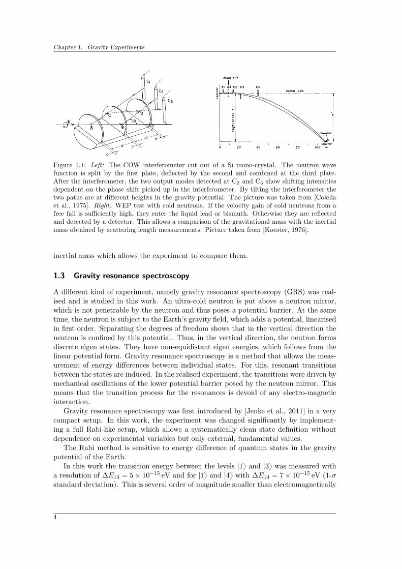
The COW experiment [Colella et al., 1975] measured the gravitational phase shift ofa neutron in an interferometric setup. A neutron wave function is split on a silicon plate,then deflected at a subsequent plate and finally combined again by a third plate (seefigure 1.1). The output modes show the interfered signal from the two parts. Any phasedifference that is accumulated by the wave function in the two separate ways results inintensity being moved from one output mode to the other. By tilting the silicon interfer-ometer one path lays higher in the gravitational potential than the other, which leads toa gravitational phase shift β proportional to wave length, local acceleration and neutronmass: β9λg~´2m2
N (as well as known and unknown systematic effects like the phaseshift due to bending of the material). This shows that the quantum particle behavesindeed as expected in the gravity field. The same method can be used in atomic interfer-ometers, which are implemented in various laboratories [Peters et al., 1999, Chiow et al.,2011, Hamilton et al., 2015a]. There, instead of neutrons, laser-cooled atomic ensemblesare separated and combined again in a gravitational field. The separation, deflection andcombination are here realised by laser pulses and the population of the output modes isdetermined by fluorescence. A modification of the scheme is an implementation wheresuch an atom interferometer setup is dropped in a drop tower [Schlippert et al., 2014].During the free fall two atom clouds of different composition are each interfered simul-taneously and the weak equivalence principle (WEP) can be tested.
Very slow free-falling neutrons were used to test the WEP [Koester, 1976] (see figure1.1 right). The kinetic energy gain from the fall needed to penetrate liquid lead andbismuth was measured and their scattering length derived. This method was compared toscattering-length measurements independent of gravity. While the first method includesthe gravitational mass, the other results were only dependent on the inertial mass.
More recently, ultra-cold neutrons were used to study the weak equivalence principle[Frank et al., 2009]. Monochromatic neutrons, produced by a spectrometer, fell downin the gravity potential and passed subsequently a rotating grating. The grating de-creased their kinetic energy by a quantised amount depending on the diffraction order.Afterwards the neutrons encountered an energy selector, which accepted the same en-ergy as the initial spectrometer. Neutrons could only pass the experiment when thekinetic energy gain from the fall compensated the energy loss of the grating. To fulfilthis condition, the vertical position of the final spectrometer could be changed as wellas the rotation frequency of the grating. While the energy gain from the classical fall isdependent on the gravitational mass, the energy loss at the grating is a function of the
3
Chapter 1. Gravity Experiments
PHYSICAL REVIEW D VOLUME 14, NUMBER 4 15 AUGUST 1976
Verification of the equivalence of gravitational and inertial mass for the neutron
L. KoesterPhysik-Department der Technischen Universitat 3funchen, Reaktorstation Garching, Munich, Germany
(Received 2 February 1976)A comparison of neutron scattering lengths measured dependent on and independent of gravity leads to avalue y for the ratio of gravitational to inertial mass for the neutron. We obtained y = 1.00016+0.00025. Thismeans the first verification of the equivalence for the neutron with an uncertainty of only 1/4000.
I. INTRODUCTION
Very precise measurements of the gravitationalforce have been performed only on bulk matter"'and most recently on very massive bodies' . Bythese experiments the principle of equivalence ofinertial and gravitational mass could be verifiedwithin stringent limits of 2 parts in 10' . Further-more, it has been shown that the gravity acceler-ation is independent of the composition of matterwithin one part in 10".' Thus it may be concludedthat neutrons and protons bound in nuclei experi-ence the same gravitational acceleration withinabout 10 "4g/g. On the other hand the behaviorof free particles, atoms, ' neutrons, ""'electrons, 'and photons" in the earth's gravitational field hasbeen studied with lower accuracy of about onlyone part in 10' or 10'. Among the particles, theneutron is best suited for a study of the gravitation-al force in the "quantum limit"" since it may ex-perience the gravity simultaneously while reactingas a matter wave.Thus, experiments with freely falling matter
waves may provide a direct proof of the statementthat the action of gravity does not affect the valid-ity of the quantum physical laws for matter waves.A verification of this fact includes also the verifi-cation of the Einstein equivalence principle. On theother hand, experiments with freely falling neu-trons in the "classical" limit, without neutron re-actions other than simple detection, are not suit-able for verifying the equivalence.In this note I will report on evaluations of exact
measurements of scattering length for slow neu-trons which led to a direct verification of theequivalence for the neutron in the quantum limit.
for the equality of inertial (m;) and passive gravi-tational mass (m) for the neutron. A verificationof this equality with y =1 would confirm that theuniversality of free fall implies the Einsteinequivalence principle since gz/g, =m/m, . Suitablefor this purpose are experiments which have beenperformed to measure neutron scattering lengthsdependent on and independent of gravity. Thegravity-dependent measurements were made in theneutron gravity ref ractometer. ' ' In this device(see Fig. 1) very slow neutrons are reflected fromliquid mirrors after having fallen a distance h.By the free fall they gain an energy mgfh in thedirection of gravity. If this energy equals thepotential energy of neutrons inside the mirrorsubstance (scattering length b, N atoms per cm')the relation
m ain slit
K1 K3 K2 K5-„t0 9 0."or a ~K4
beam axis
m g,h, = 2~5'm. -'Nb
is valid. h, denotes the critical height for totalreflection. Measurements of h, for liquid lead'and previous experiments" on liquid bismuthyielded values for the scattering length bf listedin line 12 of Table I. These quantities were cal-culated with effective values h,* for the criticalheight of fall" according to
Nb& ——m, mg&h,*/2vh' = ym~ ,g,*h2/sv'.The equivalence fa.ctor y = (m,./m)(gz/g, ) was takento be unity. If this assumption is not fulfilled,
II. METHOD AND RESULT
From the experimentally (with high accuracy)confirmed principle of the universality of freefall it follows that the gravitational accelerationsof the free neutron (gz) and of bulk matter, thelocal value (g,), are equal. Thus, neutron ex-periments which result in a value for the equi-valence factor y = (m, /m)(gz/g, ) provide a test
0O
Ch
1F
I I I I I I I I mirror0 20 40 60 80 100 m
FIG. 1. Principle of the neutron gravity refractometer.Kl, ... , Kg: slits and stopper for the neutron beam(Ref. 8).
14 907
Figure 1.1: Left: The COW interferometer cut out of a Si mono-crystal. The neutron wavefunction is split by the first plate, deflected by the second and combined at the third plate.After the interferometer, the two output modes detected at C2 and C3 show shifting intensitiesdependent on the phase shift picked up in the interferometer. By tilting the interferometer thetwo paths are at different heights in the gravity potential. The picture was taken from [Colellaet al., 1975]. Right: WEP test with cold neutrons. If the velocity gain of cold neutrons from afree fall is sufficiently high, they enter the liquid lead or bismuth. Otherwise they are reflectedand detected by a detector. This allows a comparison of the gravitational mass with the inertialmass obtained by scattering length measurements. Picture taken from [Koester, 1976].
inertial mass which allows the experiment to compare them.
1.3 Gravity resonance spectroscopy
A different kind of experiment, namely gravity resonance spectroscopy (GRS) was real-ised and is studied in this work. An ultra-cold neutron is put above a neutron mirror,which is not penetrable by the neutron and thus poses a potential barrier. At the sametime, the neutron is subject to the Earth’s gravity field, which adds a potential, linearisedin first order. Separating the degrees of freedom shows that in the vertical direction theneutron is confined by this potential. Thus, in the vertical direction, the neutron formsdiscrete eigen states. They have non-equidistant eigen energies, which follows from thelinear potential form. Gravity resonance spectroscopy is a method that allows the meas-urement of energy differences between individual states. For this, resonant transitionsbetween the states are induced. In the realised experiment, the transitions were driven bymechanical oscillations of the lower potential barrier posed by the neutron mirror. Thismeans that the transition process for the resonances is devoid of any electro-magneticinteraction.
Gravity resonance spectroscopy was first introduced by [Jenke et al., 2011] in a verycompact setup. In this work, the experiment was changed significantly by implement-ing a full Rabi-like setup, which allows a systematically clean state definition withoutdependence on experimental variables but only external, fundamental values.
The Rabi method is sensitive to energy difference of quantum states in the gravitypotential of the Earth.
In this work the transition energy between the levels |1y and |3y was measured witha resolution of ∆E13 “ 5ˆ 10´15 eV and for |1y and |4y with ∆E14 “ 7ˆ 10´15 eV (1-σstandard deviation). This is several order of magnitude smaller than electromagnetically
4
1.3. Gravity resonance spectroscopy
bound states. In the long run a sensitivity of 5ˆ 10´21 eV can be expected [Abele et al.,2010].
While GRS also uses a quantum system within a gravitational field in the Newtonianlimit, the experiment is unique in the way that gravitation enters the system. Forother experiments, gravity becomes detectable through an induced phase shift or dueto an energy gain of the quantum particle. Here however, the properties of the systemthemselves are defined by the gravitational field. As a consequence, gravitation is notthe reason for one effect among others that leads to a measurable change in a physicalquantity, but instead defines the whole system. Consequently, hypothetical modificationsof general relativity do not just lead to deviations of one effect among many, but to bethe main effect that can be studied in a systematically simpler form.
Gravity resonance spectroscopy has access to a number of parameters which allowto study gravity with different aspects. These experimental parameters are distance,mass, torsion, spin-coupling and the cosmological constant. A summary can be foundin table 1.1. Focusing on the distance allows to test the validity of Newton’s inversesquare law at short distances. Most new physics models predict additional quantumfields which exhibit characteristic length dependencies of a Yukawa-like potential. Thesearch for such models that modify the distance dependency is discussed in section 5.3.Next, both the inertial and the gravitational mass enter the description of our system,but on a different footing, which allows a test of the universal free fall, which is animportant part of the Einstein equivalence principle which itself is a cornerstone of GR.Additionally, this test is not with a classical but a quantum system. In section 5.2 it willbe discussed how GRS can contribute to this topic. Next, cosmological models with ascreening mechanism, like the hypothetical chameleon field, can in principle be detectedwith GRS. Derived limits on this special scalar-field can be found in section 5.4. GRScan also search for modifications of the gravitational potential caused by (pseudo-)scalarcouplings of neutrons with axion-like particles, which are dark matter candidates. Thishas been demonstrated in the previous iteration of the experiment [Jenke et al., 2014] anda technical analysis of a component, namely the spin-selector can be found in appendixB. For completeness, it should be mentioned that theoretically GRS has the means tosearch for torsion, a geometrical concept beyond GR, as it would result to a metric-spincoupling of the neutron. This has not been tested with this setup but further discussioncan be found in [Abele et al., 2015].
5
Chapter 1. Gravity Experiments
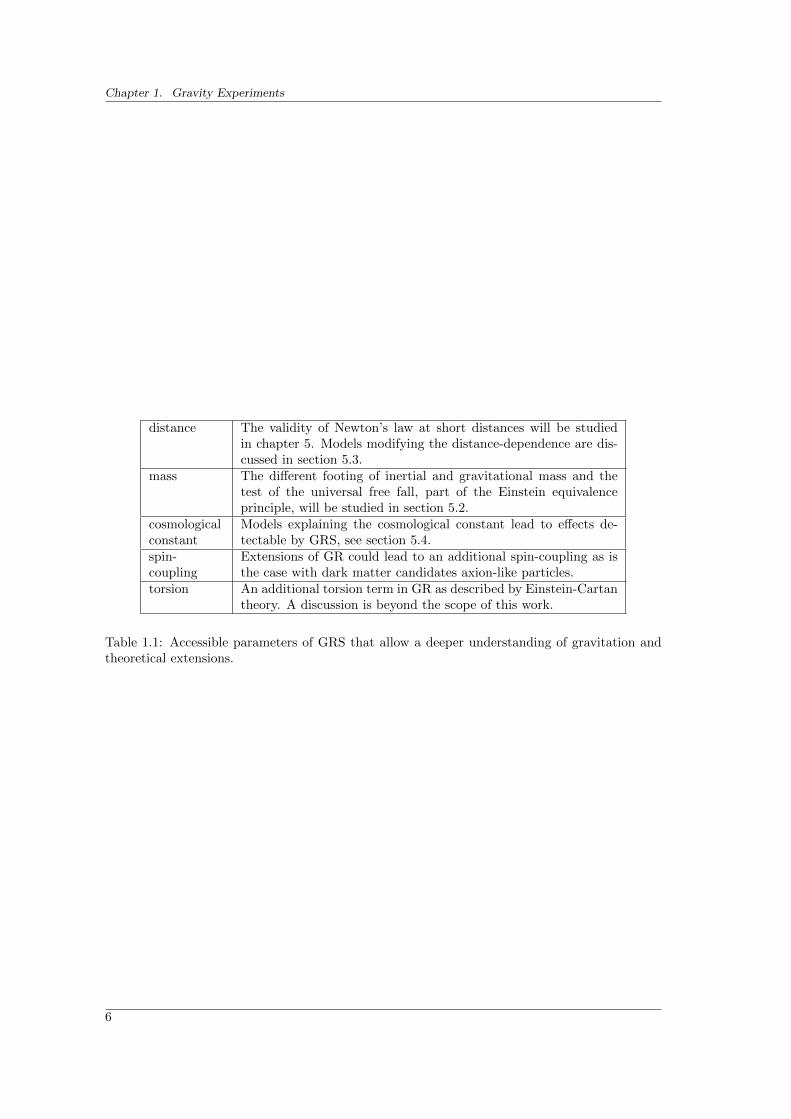
distance The validity of Newton’s law at short distances will be studiedin chapter 5. Models modifying the distance-dependence are dis-cussed in section 5.3.
mass The different footing of inertial and gravitational mass and thetest of the universal free fall, part of the Einstein equivalenceprinciple, will be studied in section 5.2.
cosmologicalconstant
Models explaining the cosmological constant lead to effects de-tectable by GRS, see section 5.4.
spin-coupling
Extensions of GR could lead to an additional spin-coupling as isthe case with dark matter candidates axion-like particles.
torsion An additional torsion term in GR as described by Einstein-Cartantheory. A discussion is beyond the scope of this work.
Table 1.1: Accessible parameters of GRS that allow a deeper understanding of gravitation andtheoretical extensions.
6
Chapter 2
Gravity tests using Resonance Spectroscopy
2.1 Ultra-cold neutrons
While there are many quantum objects to study gravity, the properties of ultra-coldneutrons make them ideal probes. Neutrons below a critically energy of about 300 neV(depending on the material) are reflected totally under any angle of incidence from mostsurfaces, they are then called ultra-cold neutrons (UCNs). This effect occurs when thewave length of the neutron is large enough to be be coherently scattered by the nuclei ofthe bulk. The bulk can then be described by an effective Fermi potential VF which wasintroduced by Fermi in 1936 [Golub et al., 1991]:
VF “2π~2
mNnbc, (2.1)
where mN is the neutron mass, bc the coherent scattering length of the material andn the material density. The neutron with a kinetic energy below VF has an exponen-tially decaying probability of penetrating the bulk and is thus reflected from the surface.Typical values for the Fermi potential of different materials are VF «p50 to 500q neV.
First ultra-cold neutrons were produced at Munich, Germany, and in Dubna, Russia,by [Steyerl, 1969, Lushchikov et al., 1969]. They can be produced in fission reactorslike FRM-II in Munich and the high-flux reactor at the Institut Laue-Langevin (ILL)in Grenoble, which delivers the highest UCN density. At the ILL, UCNs are obtainedthrough multiple steps: Neutrons from the reactor core are thermalised in a cold sourcefilled with liquid deuterium. Afterwards they ascend in a neutron guide against gravityreducing their kinetic energy. By sending them through a Doppler-cooling turbine, de-veloped by Steyerl [Steyerl, 1975] their velocity is reduced down to „p5 to 10qm s´1. Theultra-cold neutrons are then fed through neutron guides and are available for experimentsin a steady-flow mode. Alternative approaches use super-thermal neutron sources whichemploy down-scattering of cold neutrons in super-fluid helium He4 [Zimmer et al., 2011]and spallation sources in combination with down-scattering in solid deuterium e.g. atthe Paul Scherrer Institut [Anghel et al., 2009].
Ultra-cold neutrons found numerous applications in various experiments due to theirproperties. Currently the best limits on the neutrons electric dipole moment (nEDM)
7
Chapter 2. Gravity tests using Resonance Spectroscopy
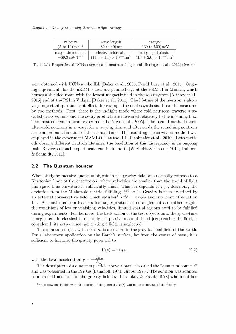
velocity wave length energyp5 to 10qm s´1 p80 to 40qnm p130 to 500qneV
magnetic moment electr. polarisab. magn. polarisab.´60.3 neV T´1 p11.6˘ 1.5q ˆ 10´4 fm3 p3.7˘ 2.0q ˆ 10´4 fm3
Table 2.1: Properties of UCNs (upper) and neutrons in general [Beringer et al., 2012] (lower).
were obtained with UCNs at the ILL [Baker et al., 2006, Pendlebury et al., 2015]. Ongo-ing experiments for the nEDM search are planned e.g. at the FRM-II in Munich, whichhouses a shielded room with the lowest magnetic field in the solar system [Altarev et al.,2015] and at the PSI in Villigen [Baker et al., 2011]. The lifetime of the neutron is also avery important question as it effects for example the nucleosynthesis. It can be measuredby two methods. First, there is the in-flight mode where cold neutrons traverse a so-called decay volume and the decay products are measured relatively to the incoming flux.The most current in-beam experiment is [Nico et al., 2005]. The second method storesultra-cold neutrons in a vessel for a varying time and afterwards the remaining neutronsare counted as a function of the storage time. This counting-the-survivors method wasemployed in the experiment MAMBO II at the ILL [Pichlmaier et al., 2010]. Both meth-ods observe different neutron lifetimes, the resolution of this discrepancy is an ongoingtask. Reviews of such experiments can be found in [Wietfeldt & Greene, 2011, Dubbers& Schmidt, 2011].
2.2 The Quantum bouncer
When studying massive quantum objects in the gravity field, one normally retreats to aNewtonian limit of the description, where velocities are smaller than the speed of lightand space-time curvature is sufficiently small. This corresponds to hµν , describing thedeviation from the Minkowski metric, fulfilling |h00| ! 1. Gravity is then described byan external conservative field which satisfies1 ∇2φ “ 4πGρ and is a limit of equation1.1. As most quantum features like superposition or entanglement are rather fragile,the conditions of low or vanishing velocities, limited spatial regions need to be fulfilledduring experiments. Furthermore, the back action of the test objects onto the space-timeis neglected. In classical terms, only the passive mass of the object, sensing the field, isconsidered, its active mass, generating a field, is neglected.
The quantum object with mass m is attracted in the gravitational field of the Earth.For a laboratory application on the Earth’s surface, far from the centre of mass, it issufficient to linearise the gravity potential to
V pzq “ mg z, (2.2)
with the local acceleration g “ ´GMC
R2C
.
The description of a quantum particle above a barrier is called the ”quantum bouncer”and was presented in the 1970ies [Langhoff, 1971, Gibbs, 1975]. The solution was adaptedto ultra-cold neutrons in the gravity field by [Luschikov & Frank, 1978] who identified
1From now on, in this work the notion of the potential V prq will be used instead of the field φ.
8
2.2. The Quantum bouncer
1
2
3
4
5
0 10 20 30 40 50
1.41
2.46
3.32
4.08
4.78
height [µm]
energy
[peV
]
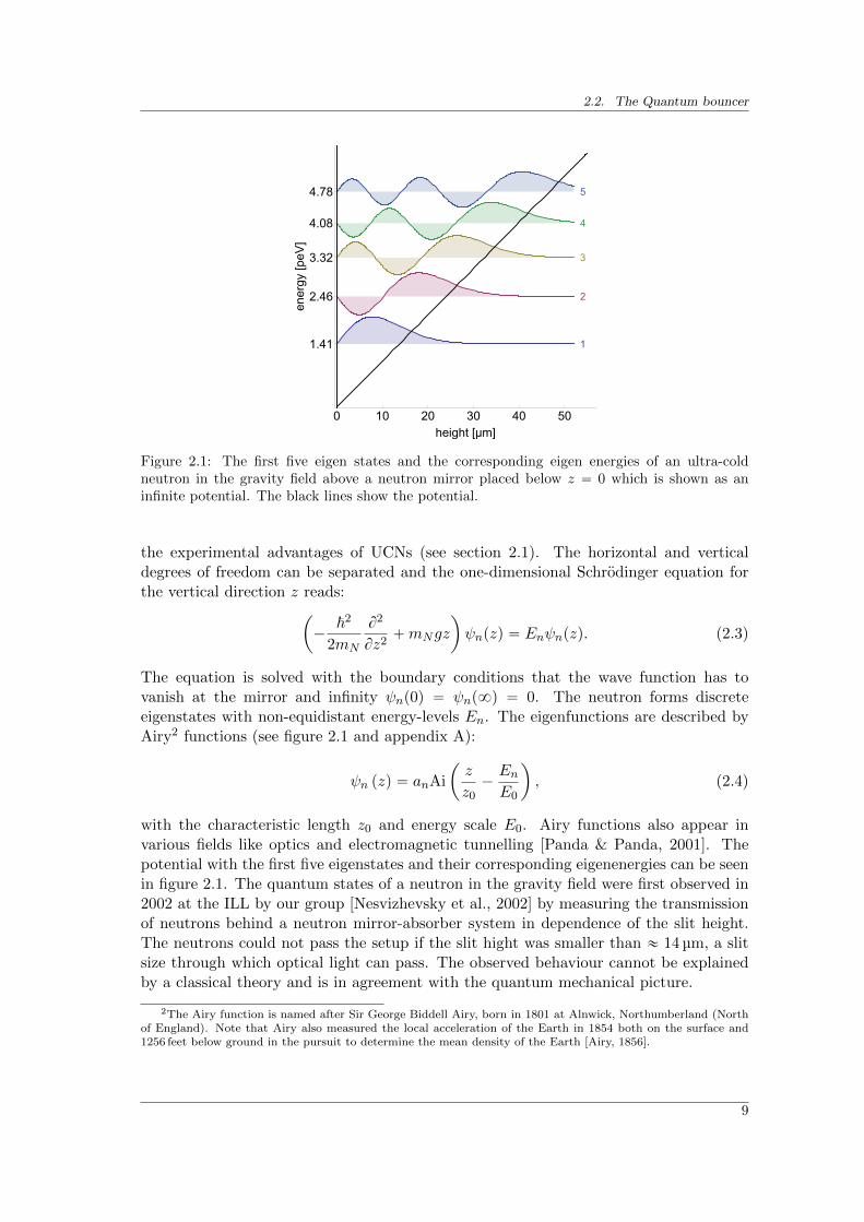
Figure 2.1: The first five eigen states and the corresponding eigen energies of an ultra-coldneutron in the gravity field above a neutron mirror placed below z “ 0 which is shown as aninfinite potential. The black lines show the potential.
the experimental advantages of UCNs (see section 2.1). The horizontal and verticaldegrees of freedom can be separated and the one-dimensional Schrodinger equation forthe vertical direction z reads:
ˆ
´~2
2mN
B2
Bz2`mNgz
˙
ψnpzq “ Enψnpzq. (2.3)
The equation is solved with the boundary conditions that the wave function has tovanish at the mirror and infinity ψnp0q “ ψnp8q “ 0. The neutron forms discreteeigenstates with non-equidistant energy-levels En. The eigenfunctions are described byAiry2 functions (see figure 2.1 and appendix A):
ψn pzq “ anAi
ˆ
z
z0´EnE0
˙
, (2.4)
with the characteristic length z0 and energy scale E0. Airy functions also appear invarious fields like optics and electromagnetic tunnelling [Panda & Panda, 2001]. Thepotential with the first five eigenstates and their corresponding eigenenergies can be seenin figure 2.1. The quantum states of a neutron in the gravity field were first observed in2002 at the ILL by our group [Nesvizhevsky et al., 2002] by measuring the transmissionof neutrons behind a neutron mirror-absorber system in dependence of the slit height.The neutrons could not pass the setup if the slit hight was smaller than « 14 µm, a slitsize through which optical light can pass. The observed behaviour cannot be explainedby a classical theory and is in agreement with the quantum mechanical picture.
2The Airy function is named after Sir George Biddell Airy, born in 1801 at Alnwick, Northumberland (Northof England). Note that Airy also measured the local acceleration of the Earth in 1854 both on the surface and1256 feet below ground in the pursuit to determine the mean density of the Earth [Airy, 1856].
9
Chapter 2. Gravity tests using Resonance Spectroscopy
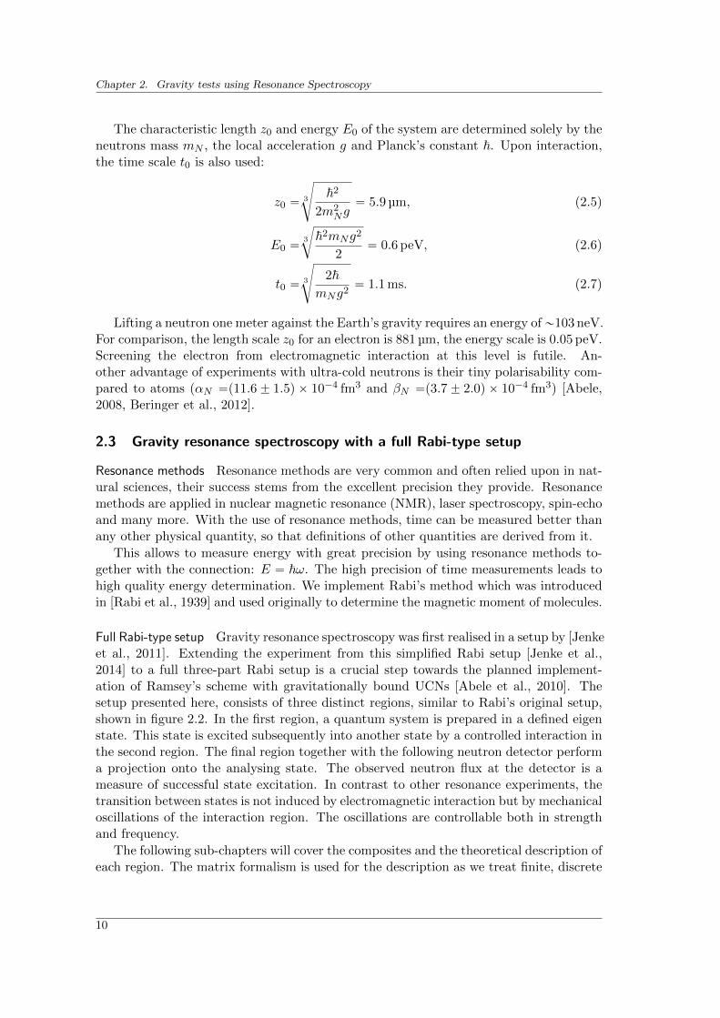
The characteristic length z0 and energy E0 of the system are determined solely by theneutrons mass mN , the local acceleration g and Planck’s constant ~. Upon interaction,the time scale t0 is also used:
z0 “3
d
~2
2m2Ng
“ 5.9 µm, (2.5)
E0 “3
c
~2mNg2
2“ 0.6 peV, (2.6)
t0 “3
d
2~mNg2
“ 1.1 ms. (2.7)
Lifting a neutron one meter against the Earth’s gravity requires an energy of„103 neV.For comparison, the length scale z0 for an electron is 881 µm, the energy scale is 0.05 peV.Screening the electron from electromagnetic interaction at this level is futile. An-other advantage of experiments with ultra-cold neutrons is their tiny polarisability com-pared to atoms (αN “p11.6˘ 1.5q ˆ 10´4 fm3 and βN “p3.7˘ 2.0q ˆ 10´4 fm3) [Abele,2008, Beringer et al., 2012].
2.3 Gravity resonance spectroscopy with a full Rabi-type setup
Resonance methods Resonance methods are very common and often relied upon in nat-ural sciences, their success stems from the excellent precision they provide. Resonancemethods are applied in nuclear magnetic resonance (NMR), laser spectroscopy, spin-echoand many more. With the use of resonance methods, time can be measured better thanany other physical quantity, so that definitions of other quantities are derived from it.
This allows to measure energy with great precision by using resonance methods to-gether with the connection: E “ ~ω. The high precision of time measurements leads tohigh quality energy determination. We implement Rabi’s method which was introducedin [Rabi et al., 1939] and used originally to determine the magnetic moment of molecules.
Full Rabi-type setup Gravity resonance spectroscopy was first realised in a setup by [Jenkeet al., 2011]. Extending the experiment from this simplified Rabi setup [Jenke et al.,2014] to a full three-part Rabi setup is a crucial step towards the planned implement-ation of Ramsey’s scheme with gravitationally bound UCNs [Abele et al., 2010]. Thesetup presented here, consists of three distinct regions, similar to Rabi’s original setup,shown in figure 2.2. In the first region, a quantum system is prepared in a defined eigenstate. This state is excited subsequently into another state by a controlled interaction inthe second region. The final region together with the following neutron detector performa projection onto the analysing state. The observed neutron flux at the detector is ameasure of successful state excitation. In contrast to other resonance experiments, thetransition between states is not induced by electromagnetic interaction but by mechanicaloscillations of the interaction region. The oscillations are controllable both in strengthand frequency.
The following sub-chapters will cover the composites and the theoretical description ofeach region. The matrix formalism is used for the description as we treat finite, discrete
10
2.3. Gravity resonance spectroscopy with a full Rabi-type setup
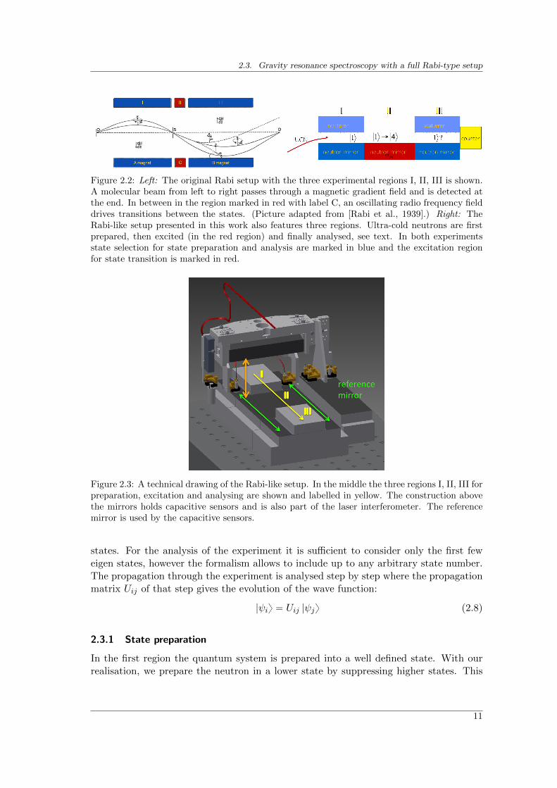
Figure 2.2: Left: The original Rabi setup with the three experimental regions I, II, III is shown.A molecular beam from left to right passes through a magnetic gradient field and is detected atthe end. In between in the region marked in red with label C, an oscillating radio frequency fielddrives transitions between the states. (Picture adapted from [Rabi et al., 1939].) Right: TheRabi-like setup presented in this work also features three regions. Ultra-cold neutrons are firstprepared, then excited (in the red region) and finally analysed, see text. In both experimentsstate selection for state preparation and analysis are marked in blue and the excitation regionfor state transition is marked in red.
Figure 2.3: A technical drawing of the Rabi-like setup. In the middle the three regions I, II, III forpreparation, excitation and analysing are shown and labelled in yellow. The construction abovethe mirrors holds capacitive sensors and is also part of the laser interferometer. The referencemirror is used by the capacitive sensors.
states. For the analysis of the experiment it is sufficient to consider only the first feweigen states, however the formalism allows to include up to any arbitrary state number.The propagation through the experiment is analysed step by step where the propagationmatrix Uij of that step gives the evolution of the wave function:
|ψiy “ Uij |ψjy (2.8)
2.3.1 State preparation
In the first region the quantum system is prepared into a well defined state. With ourrealisation, we prepare the neutron in a lower state by suppressing higher states. This
11
Chapter 2. Gravity tests using Resonance Spectroscopy
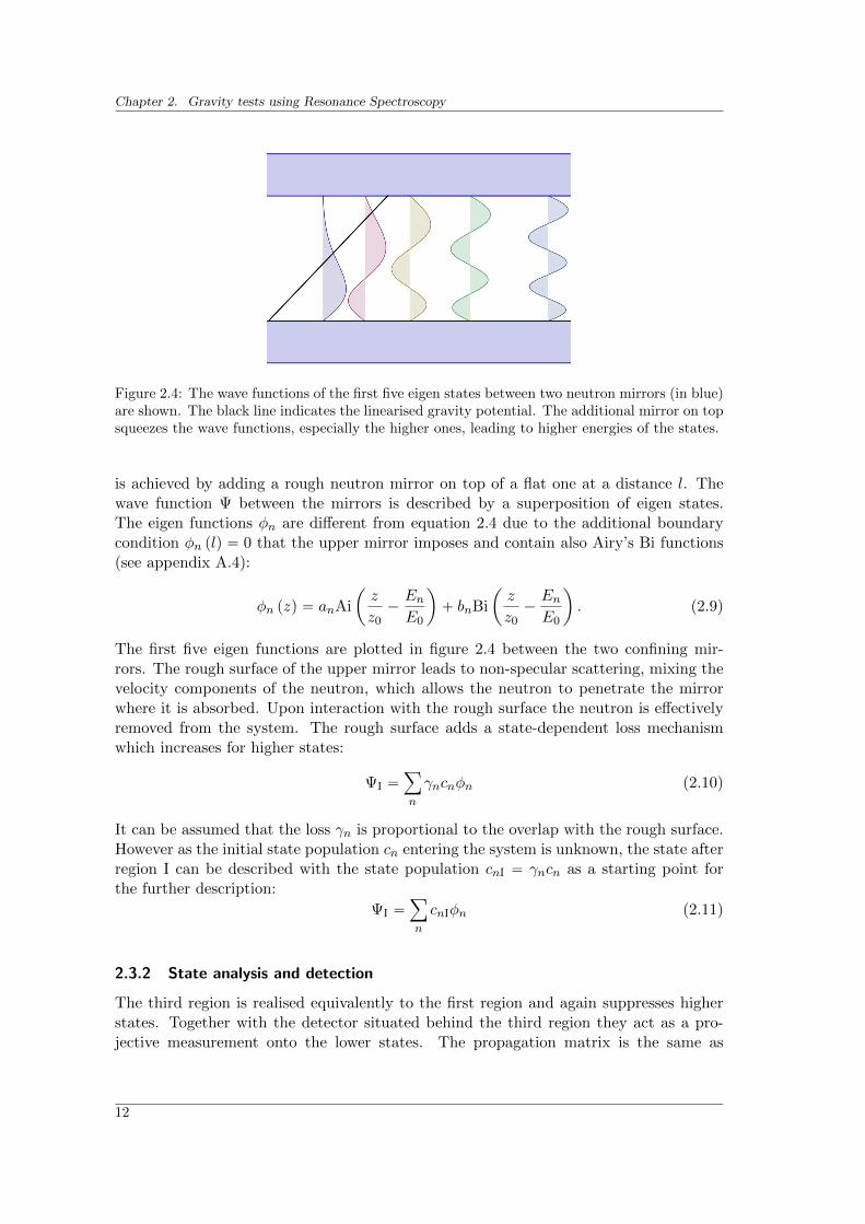
Figure 2.4: The wave functions of the first five eigen states between two neutron mirrors (in blue)are shown. The black line indicates the linearised gravity potential. The additional mirror on topsqueezes the wave functions, especially the higher ones, leading to higher energies of the states.
is achieved by adding a rough neutron mirror on top of a flat one at a distance l. Thewave function Ψ between the mirrors is described by a superposition of eigen states.The eigen functions φn are different from equation 2.4 due to the additional boundarycondition φn plq “ 0 that the upper mirror imposes and contain also Airy’s Bi functions(see appendix A.4):
φn pzq “ anAi
ˆ
z
z0´EnE0
˙
` bnBi
ˆ
z
z0´EnE0
˙
. (2.9)
The first five eigen functions are plotted in figure 2.4 between the two confining mir-rors. The rough surface of the upper mirror leads to non-specular scattering, mixing thevelocity components of the neutron, which allows the neutron to penetrate the mirrorwhere it is absorbed. Upon interaction with the rough surface the neutron is effectivelyremoved from the system. The rough surface adds a state-dependent loss mechanismwhich increases for higher states:
ΨI “ÿ
n
γncnφn (2.10)
It can be assumed that the loss γn is proportional to the overlap with the rough surface.However as the initial state population cn entering the system is unknown, the state afterregion I can be described with the state population cnI “ γncn as a starting point forthe further description:
ΨI “ÿ
n
cnIφn (2.11)
2.3.2 State analysis and detection
The third region is realised equivalently to the first region and again suppresses higherstates. Together with the detector situated behind the third region they act as a pro-jective measurement onto the lower states. The propagation matrix is the same as
12
2.3. Gravity resonance spectroscopy with a full Rabi-type setup
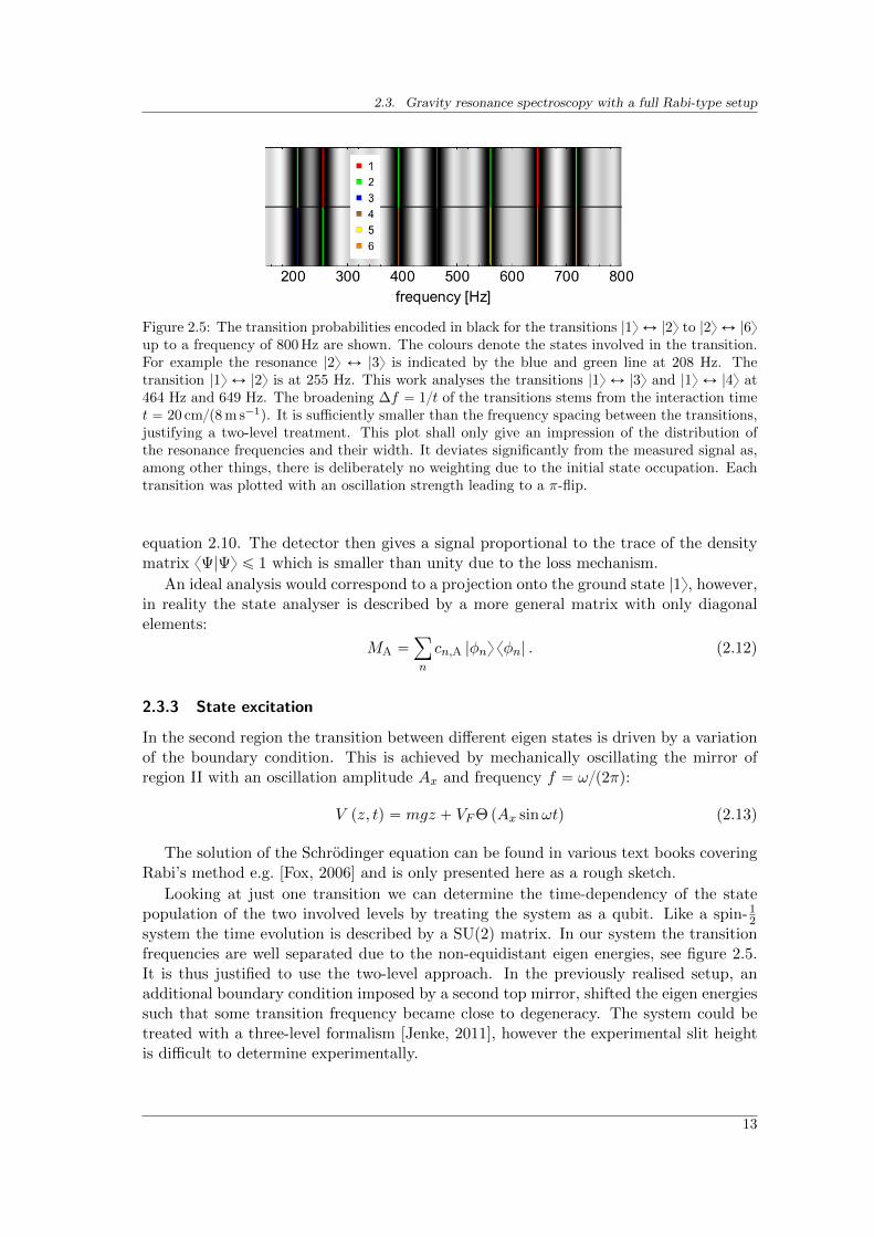
Figure 2.5: The transition probabilities encoded in black for the transitions |1y Ø |2y to |2y Ø |6yup to a frequency of 800 Hz are shown. The colours denote the states involved in the transition.For example the resonance |2y Ø |3y is indicated by the blue and green line at 208 Hz. Thetransition |1y Ø |2y is at 255 Hz. This work analyses the transitions |1y Ø |3y and |1y Ø |4y at464 Hz and 649 Hz. The broadening ∆f “ 1t of the transitions stems from the interaction timet “ 20 cmp8 m s´1q. It is sufficiently smaller than the frequency spacing between the transitions,justifying a two-level treatment. This plot shall only give an impression of the distribution ofthe resonance frequencies and their width. It deviates significantly from the measured signal as,among other things, there is deliberately no weighting due to the initial state occupation. Eachtransition was plotted with an oscillation strength leading to a π-flip.
equation 2.10. The detector then gives a signal proportional to the trace of the densitymatrix xΨ|Ψy ď 1 which is smaller than unity due to the loss mechanism.
An ideal analysis would correspond to a projection onto the ground state |1y, however,in reality the state analyser is described by a more general matrix with only diagonalelements:
MA “ÿ
n
cn,A |φny xφn| . (2.12)
2.3.3 State excitation
In the second region the transition between different eigen states is driven by a variationof the boundary condition. This is achieved by mechanically oscillating the mirror ofregion II with an oscillation amplitude Ax and frequency f “ ωp2πq:
V pz, tq “ mgz ` VFΘ pAx sinωtq (2.13)
The solution of the Schrodinger equation can be found in various text books coveringRabi’s method e.g. [Fox, 2006] and is only presented here as a rough sketch.
Looking at just one transition we can determine the time-dependency of the statepopulation of the two involved levels by treating the system as a qubit. Like a spin-1
2system the time evolution is described by a SU(2) matrix. In our system the transitionfrequencies are well separated due to the non-equidistant eigen energies, see figure 2.5.It is thus justified to use the two-level approach. In the previously realised setup, anadditional boundary condition imposed by a second top mirror, shifted the eigen energiessuch that some transition frequency became close to degeneracy. The system could betreated with a three-level formalism [Jenke, 2011], however the experimental slit heightis difficult to determine experimentally.
13
Chapter 2. Gravity tests using Resonance Spectroscopy
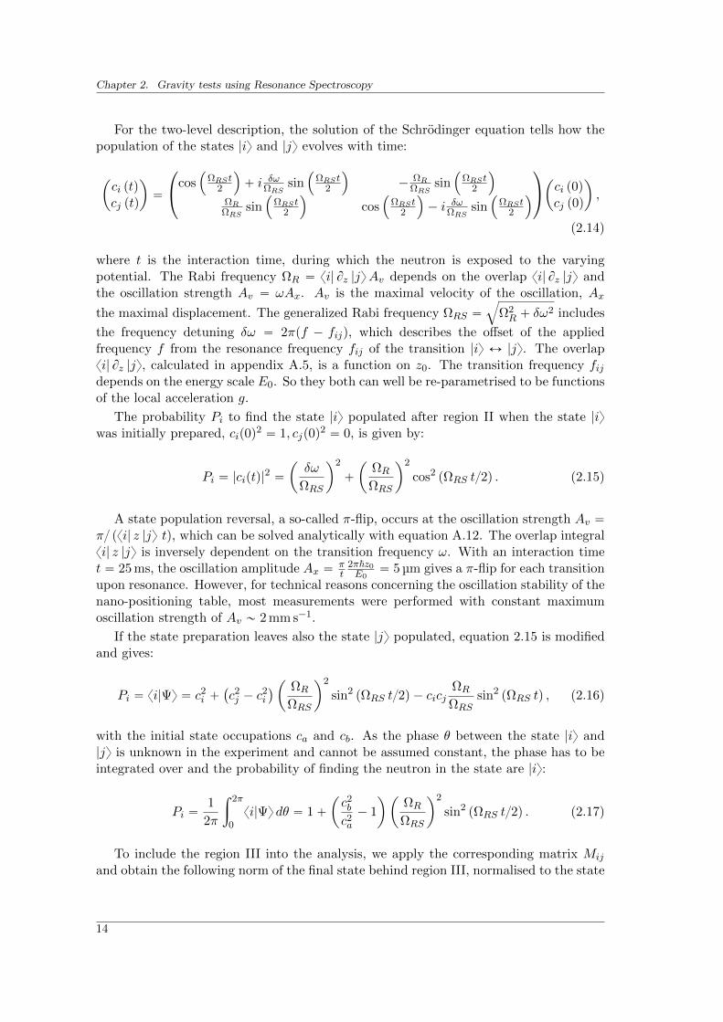
For the two-level description, the solution of the Schrodinger equation tells how thepopulation of the states |iy and |jy evolves with time:
ˆ
ci ptqcj ptq
˙
“
¨
˝
cos´
ΩRSt2
¯
` i δωΩRSsin
´
ΩRSt2
¯
´ΩR
ΩRSsin
´
ΩRSt2
¯
ΩRΩRS
sin´
ΩRSt2
¯
cos´
ΩRSt2
¯
´ i δωΩRSsin
´
ΩRSt2
¯
˛
‚
ˆ
ci p0qcj p0q
˙
,
(2.14)
where t is the interaction time, during which the neutron is exposed to the varyingpotential. The Rabi frequency ΩR “ xi| Bz |jyAv depends on the overlap xi| Bz |jy andthe oscillation strength Av “ ωAx. Av is the maximal velocity of the oscillation, Ax
the maximal displacement. The generalized Rabi frequency ΩRS “
b
Ω2R ` δω
2 includes
the frequency detuning δω “ 2πpf ´ fijq, which describes the offset of the appliedfrequency f from the resonance frequency fij of the transition |iy Ø |jy. The overlapxi| Bz |jy, calculated in appendix A.5, is a function on z0. The transition frequency fijdepends on the energy scale E0. So they both can well be re-parametrised to be functionsof the local acceleration g.
The probability Pi to find the state |iy populated after region II when the state |iywas initially prepared, cip0q
2 “ 1, cjp0q2 “ 0, is given by:
Pi “ |ciptq|2 “
ˆ
δω
ΩRS
˙2
`
ˆ
ΩR
ΩRS
˙2
cos2 pΩRS t2q . (2.15)
A state population reversal, a so-called π-flip, occurs at the oscillation strength Av “π pxi| z |jy tq, which can be solved analytically with equation A.12. The overlap integralxi| z |jy is inversely dependent on the transition frequency ω. With an interaction timet “ 25 ms, the oscillation amplitude Ax “
πt
2π~z0E0
“ 5 µm gives a π-flip for each transitionupon resonance. However, for technical reasons concerning the oscillation stability of thenano-positioning table, most measurements were performed with constant maximumoscillation strength of Av „ 2 mm s´1.
If the state preparation leaves also the state |jy populated, equation 2.15 is modifiedand gives:
Pi “ xi|Ψy “ c2i `
`
c2j ´ c
2i
˘
ˆ
ΩR
ΩRS
˙2
sin2 pΩRS t2q ´ cicjΩR
ΩRSsin2 pΩRS tq , (2.16)
with the initial state occupations ca and cb. As the phase θ between the state |iy and|jy is unknown in the experiment and cannot be assumed constant, the phase has to beintegrated over and the probability of finding the neutron in the state are |iy:
Pi “1
2π
ż 2π
0xi|Ψy dθ “ 1`
ˆ
c2b
c2a
´ 1
˙ˆ
ΩR
ΩRS
˙2
sin2 pΩRS t2q . (2.17)
To include the region III into the analysis, we apply the corresponding matrix Mij
and obtain the following norm of the final state behind region III, normalised to the state
14
2.3. Gravity resonance spectroscopy with a full Rabi-type setup
before region II:
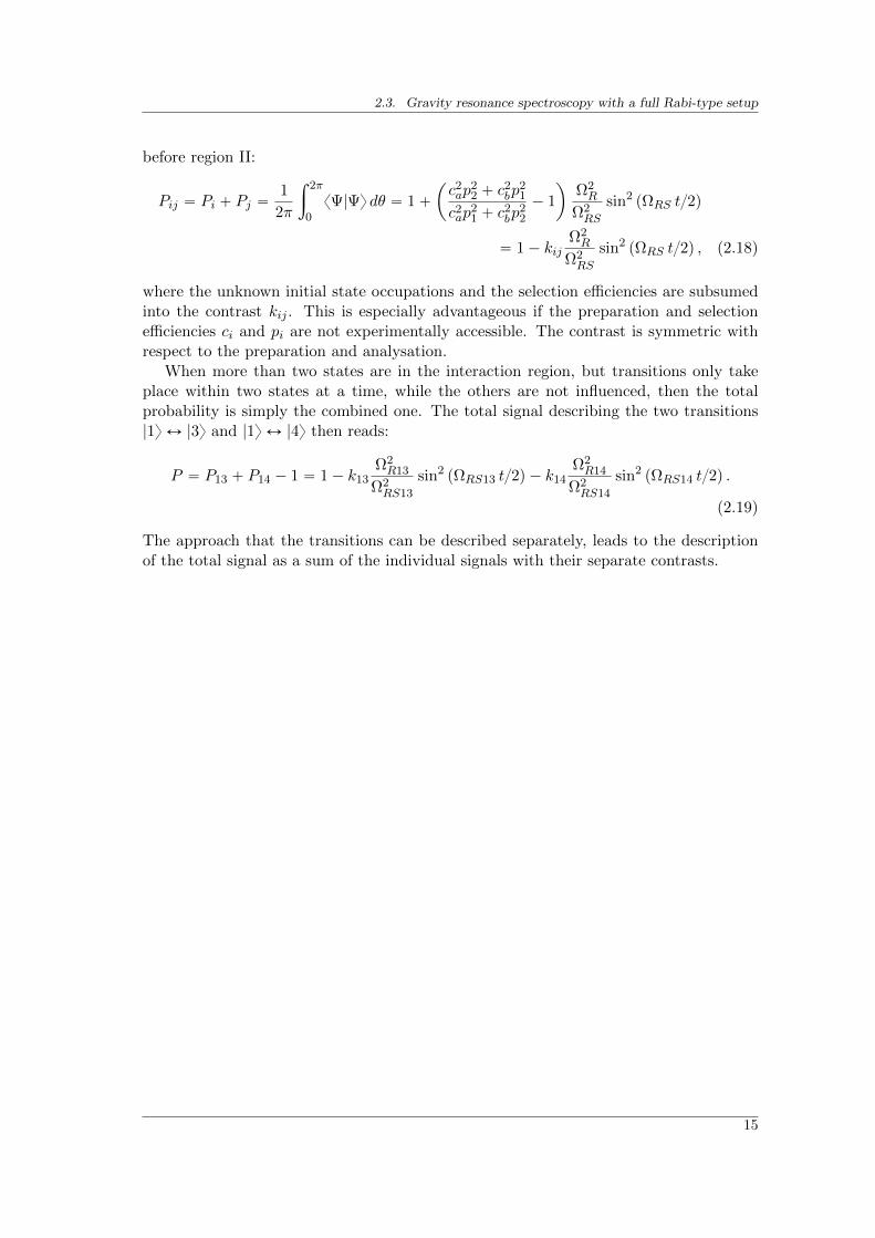
Pij “ Pi ` Pj “1
2π
ż 2π
0xΨ|Ψy dθ “ 1`
ˆ
c2ap
22 ` c
2bp
21
c2ap
21 ` c
2bp
22
´ 1
˙
Ω2R
Ω2RS
sin2 pΩRS t2q
“ 1´ kijΩ2R
Ω2RS
sin2 pΩRS t2q , (2.18)
where the unknown initial state occupations and the selection efficiencies are subsumedinto the contrast kij . This is especially advantageous if the preparation and selectionefficiencies ci and pi are not experimentally accessible. The contrast is symmetric withrespect to the preparation and analysation.
When more than two states are in the interaction region, but transitions only takeplace within two states at a time, while the others are not influenced, then the totalprobability is simply the combined one. The total signal describing the two transitions|1y Ø |3y and |1y Ø |4y then reads:
P “ P13 ` P14 ´ 1 “ 1´ k13Ω2R13
Ω2RS13
sin2 pΩRS13 t2q ´ k14Ω2R14
Ω2RS14
sin2 pΩRS14 t2q .
(2.19)
The approach that the transitions can be described separately, leads to the descriptionof the total signal as a sum of the individual signals with their separate contrasts.
15

Chapter 3
Experimental realisation of Rabi-type GRS
The measurements presented in this work were performed at the UCN beam line atthe PF2 platform of the Institut Laue-Langevin1 (ILL), which is known for its high-fluxneutron-source reactor. We were allocated the experiment number 3-14-305 which wasscheduled during the reactor cycles 167 and 168 from 28.08.-12.11.2012. In between thetwo cycles there was a planned reactor shut down for a fuel rod change. After settingup the experiment and performing various tests on the parts of the setup and initialpreparations we started measuring the transmission of neutrons through the full 3-partRabi setup as a function of the oscillation frequency and amplitude.
In this chapter, the various components of the experiment, as used during the beamtime, are presented and their physical implications are discussed in detail. The methods,like the velocity selection of ultra-cold neutrons (UCNs) and the preparation of thequantum system, are theoretically studied and evaluated. It is followed by a discussionof the realisation for induced state transitions. Afterwards, the driving and monitoringof the mechanical oscillations is discussed. The methods of neutron detection used in theexperiment are presented and followed by a discussion of the obstacles with the setupalignment and ways of dealing with them. The vacuum chamber and its purpose arementioned briefly. The observed rate dampening concludes the chapter together with ananalysis of external influences such as the moon and the rotation of the Earth.
3.1 Technical realisation and its systematic investigations
3.1.1 Neutrons time-of-flight
Selecting trajectories with Collimating blades
The experiment is of the so-called ”flow-through” type, meaning that the neutrons passthrough our setup horizontally. The aim is that the neutrons form bound quantum statesclose to the ground state with transversal energies in the pico-eV regime. Controllingand determining their horizontal velocity while preparing them at the same time in avertical quantum state is the task of the velocity selector.
1http://www.ill.eu
17
Chapter 3. Experimental realisation of Rabi-type GRS
X
Zl
x
z
mirror
scatterer
upper blade
lower blade
Zu
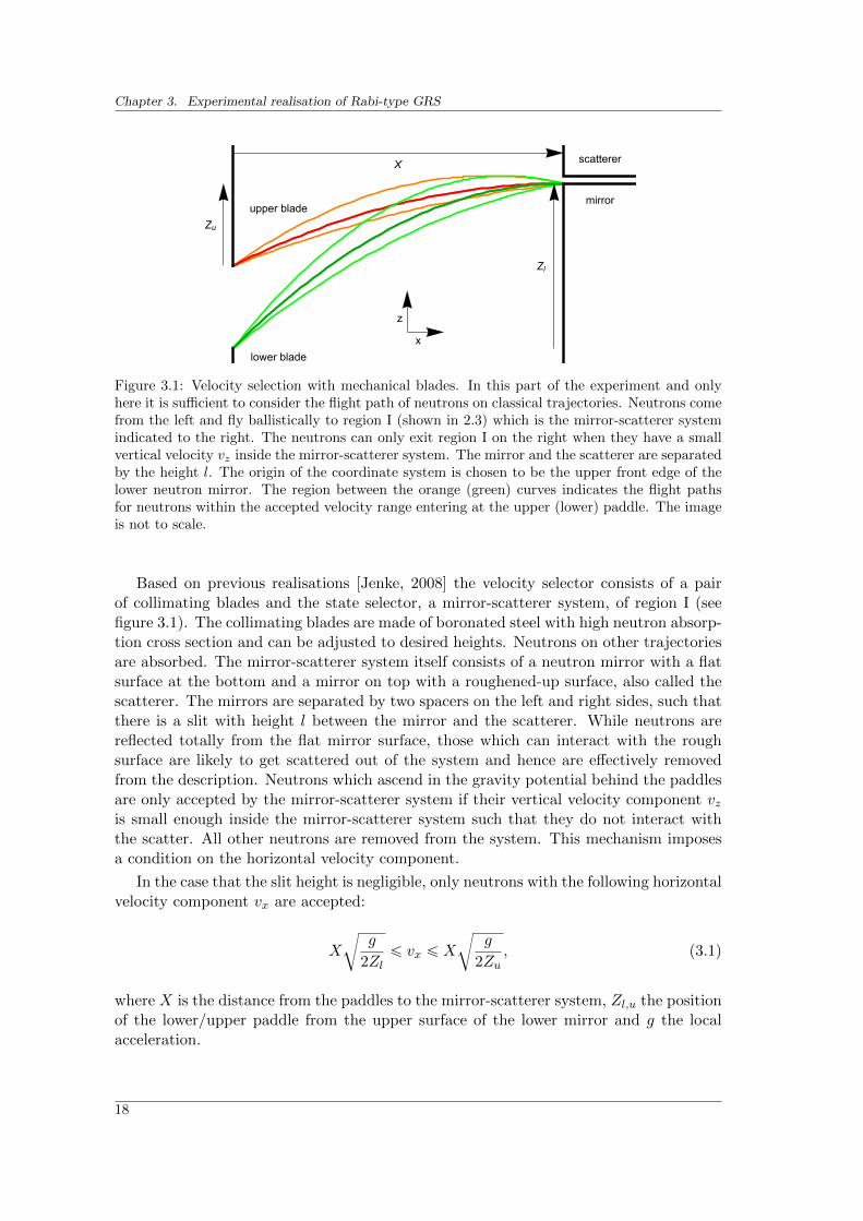
Figure 3.1: Velocity selection with mechanical blades. In this part of the experiment and onlyhere it is sufficient to consider the flight path of neutrons on classical trajectories. Neutrons comefrom the left and fly ballistically to region I (shown in 2.3) which is the mirror-scatterer systemindicated to the right. The neutrons can only exit region I on the right when they have a smallvertical velocity vz inside the mirror-scatterer system. The mirror and the scatterer are separatedby the height l. The origin of the coordinate system is chosen to be the upper front edge of thelower neutron mirror. The region between the orange (green) curves indicates the flight pathsfor neutrons within the accepted velocity range entering at the upper (lower) paddle. The imageis not to scale.
Based on previous realisations [Jenke, 2008] the velocity selector consists of a pairof collimating blades and the state selector, a mirror-scatterer system, of region I (seefigure 3.1). The collimating blades are made of boronated steel with high neutron absorp-tion cross section and can be adjusted to desired heights. Neutrons on other trajectoriesare absorbed. The mirror-scatterer system itself consists of a neutron mirror with a flatsurface at the bottom and a mirror on top with a roughened-up surface, also called thescatterer. The mirrors are separated by two spacers on the left and right sides, such thatthere is a slit with height l between the mirror and the scatterer. While neutrons arereflected totally from the flat mirror surface, those which can interact with the roughsurface are likely to get scattered out of the system and hence are effectively removedfrom the description. Neutrons which ascend in the gravity potential behind the paddlesare only accepted by the mirror-scatterer system if their vertical velocity component vzis small enough inside the mirror-scatterer system such that they do not interact withthe scatter. All other neutrons are removed from the system. This mechanism imposesa condition on the horizontal velocity component.
In the case that the slit height is negligible, only neutrons with the following horizontalvelocity component vx are accepted:
X
c
g
2Zlď vx ď X
c
g
2Zu, (3.1)
where X is the distance from the paddles to the mirror-scatterer system, Zl,u the positionof the lower/upper paddle from the upper surface of the lower mirror and g the localacceleration.
18
3.1. Technical realisation and its systematic investigations
100 µm
30 µm
2 µm
0 5 10 150.00
0.05
0.10
0.15
0.20
0.25
vx [m/s]
ξ(vx)
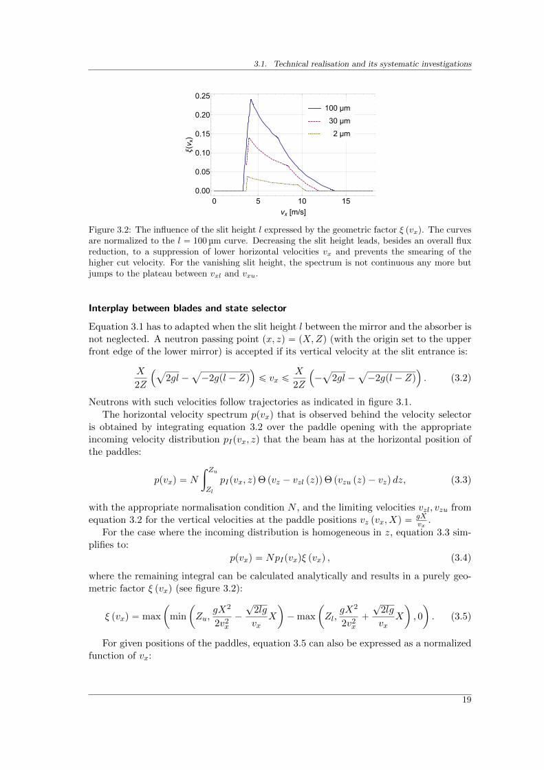
Figure 3.2: The influence of the slit height l expressed by the geometric factor ξ pvxq. The curvesare normalized to the l “ 100 µm curve. Decreasing the slit height leads, besides an overall fluxreduction, to a suppression of lower horizontal velocities vx and prevents the smearing of thehigher cut velocity. For the vanishing slit height, the spectrum is not continuous any more butjumps to the plateau between vxl and vxu.
Interplay between blades and state selector
Equation 3.1 has to adapted when the slit height l between the mirror and the absorber isnot neglected. A neutron passing point px, zq “ pX,Zq (with the origin set to the upperfront edge of the lower mirror) is accepted if its vertical velocity at the slit entrance is:
X
2Z
´
a
2gl ´a
´2gpl ´ Zq¯
ď vx ďX
2Z
´
´a
2gl ´a
´2gpl ´ Zq¯
. (3.2)
Neutrons with such velocities follow trajectories as indicated in figure 3.1.
The horizontal velocity spectrum ppvxq that is observed behind the velocity selectoris obtained by integrating equation 3.2 over the paddle opening with the appropriateincoming velocity distribution pIpvx, zq that the beam has at the horizontal position ofthe paddles:
ppvxq “ N
ż Zu
Zl
pIpvx, zqΘ pvz ´ vzl pzqqΘ pvzu pzq ´ vzq dz, (3.3)
with the appropriate normalisation condition N , and the limiting velocities vzl, vzu fromequation 3.2 for the vertical velocities at the paddle positions vz pvx, Xq “
gXvx
.
For the case where the incoming distribution is homogeneous in z, equation 3.3 sim-plifies to:
ppvxq “ NpIpvxqξ pvxq , (3.4)
where the remaining integral can be calculated analytically and results in a purely geo-metric factor ξ pvxq (see figure 3.2):
ξ pvxq “ max
ˆ
min
ˆ
Zu,gX2
2v2x
´
?2lg
vxX
˙
´max
ˆ
Zl,gX2
2v2x
`
?2lg
vxX
˙
, 0
˙
. (3.5)
For given positions of the paddles, equation 3.5 can also be expressed as a normalizedfunction of vx:
19
Chapter 3. Experimental realisation of Rabi-type GRS
vc “a
2gl, vi “Xvc
2
¨
˚
˝
ˆ
b
1´ Zll ¯ 1
˙
Zl´b
1´ Zul ¯ 1
¯
Zu
˛
‹
‚
, (3.6)
ξpvxq “1
log ZlZu
ˆ
Θ pvx ´ vIqΘ pvIII ´ vxq
ˆ
v´1x ´
gX
2vcv´2x
˙
`Θ pvx ´ vIIqΘ pvIV ´ vxq
ˆ
v´1x `
gX
2vcv´2x
˙
`Θ pvx ´ vIqΘ pvII ´ vxqZlXvc
´Θ pvx ´ vIIIqΘ pvIV ´ vxqZuXvc
˙
. (3.7)
Depending on the choice of experimental values, different terms of equation 3.7 dominateand lead to either a step-like or a mainly inverse-vx form of the geometric factor. Thelog-term ensures the correct normalisation.
Simulations of a velocity selection with rough media can be found in [Chizhova et al.,2014]. Additionally, UCNs have to pass through multiple aluminium foils which cutstheir velocity spectrum at the critical velocity of aluminium. As this is around 3.2 m s´1
it has no effect on the presented experimental setup.
Application during beam time 3-14-305
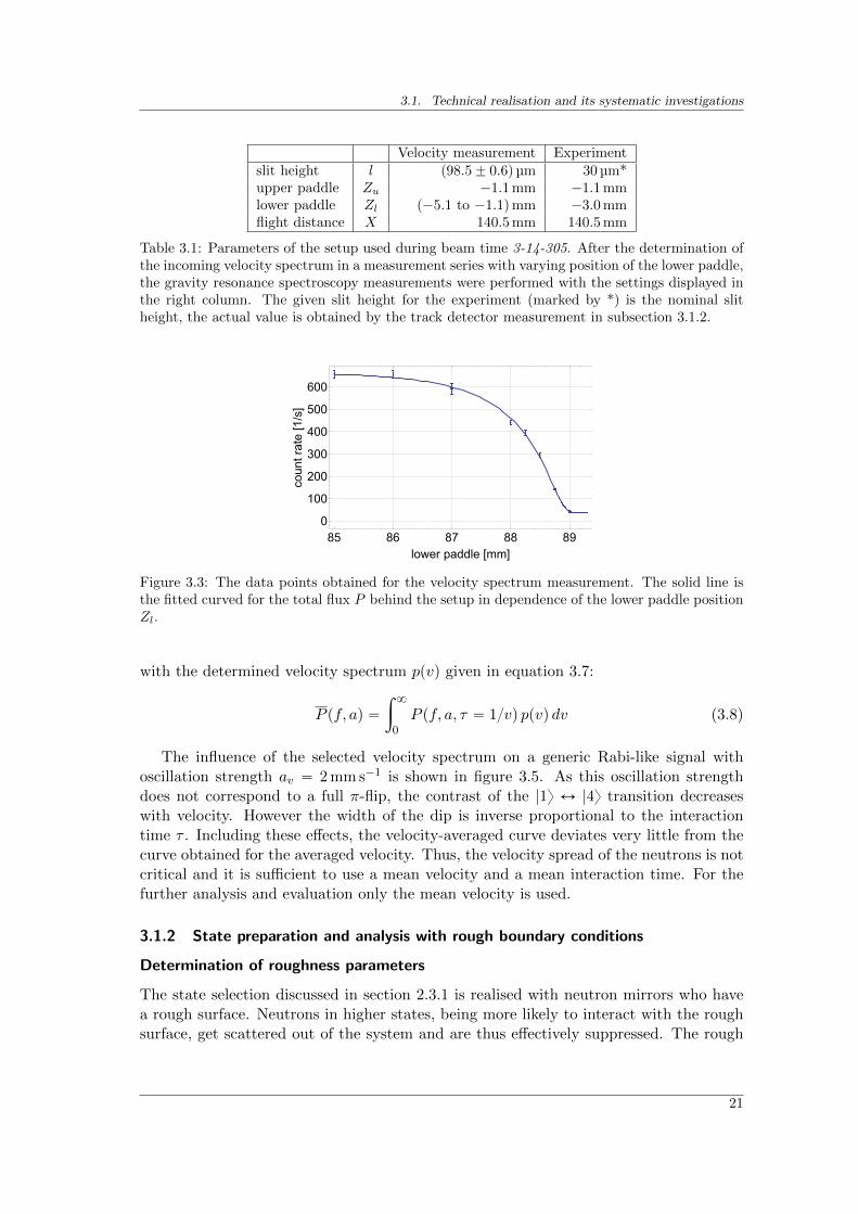
The incoming velocity spectrum was determined by a measurement set conducted inthe beginning of the beam time 3-14-305. The lower mirror had a width of 200 mm,the upper one of 100 mm, both were 150 mm long. The slit between them was set tothe height l “ p98.5˘ 0.6q µm (see table 3.1). The total flux P , being the integral ofequation 3.2, was measured as a function of the lower paddle’s position while keepingthe upper paddle fixed (see figure 3.3).
The incoming velocity distribution pI pvxq was assumed to be a polynomial of orderfour with six independent parameters. The total flux P was integrated analytically for allmeasured values of the lower paddle position. By fitting P with the least-square method,by minimizing the χ2, the values for the parameters were obtained. Figure 3.3 showsthe measurement together with the fitted curve. The velocity distribution during theexperiment can now be calculated analytically by applying the corresponding geometricalfactor for the paddle values and slit size to be found in table 3.1 (see Figure 3.4).
The final settings for the beam time 3-14-305 are displayed in table 3.1. Neglectingthe slit width between the mirrors gives an acceptance of p5.6 to 9.5qm s´1.
Influence of the velocity spread
The interaction time τ of the neutron with the oscillating potential in region II is de-termined by the velocity vx of the neutrons. To account for the velocity spread in theexperiment, the expected Rabi-like signal displayed in section 2.3 has to be integrated
20
3.1. Technical realisation and its systematic investigations
Velocity measurement Experimentslit height l p98.5˘ 0.6q µm 30 µm*upper paddle Zu ´1.1 mm ´1.1 mmlower paddle Zl p´5.1 to ´1.1qmm ´3.0 mmflight distance X 140.5 mm 140.5 mm
Table 3.1: Parameters of the setup used during beam time 3-14-305. After the determination ofthe incoming velocity spectrum in a measurement series with varying position of the lower paddle,the gravity resonance spectroscopy measurements were performed with the settings displayed inthe right column. The given slit height for the experiment (marked by *) is the nominal slitheight, the actual value is obtained by the track detector measurement in subsection 3.1.2.
85 86 87 88 890
100
200
300
400
500
600
lower paddle [mm]
countrate[1/s]
Figure 3.3: The data points obtained for the velocity spectrum measurement. The solid line isthe fitted curved for the total flux P behind the setup in dependence of the lower paddle positionZl.
with the determined velocity spectrum ppvq given in equation 3.7:
P pf, aq “
ż 8
0P pf, a, τ “ 1vq ppvq dv (3.8)
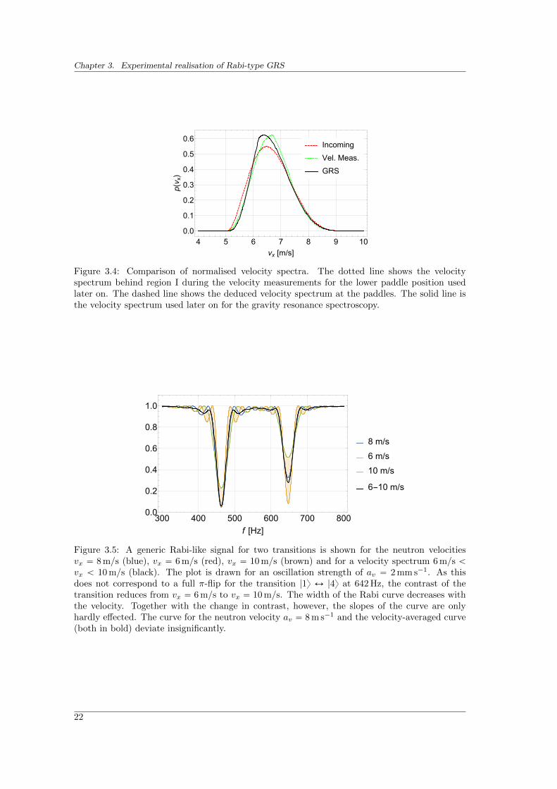
The influence of the selected velocity spectrum on a generic Rabi-like signal withoscillation strength av “ 2 mm s´1 is shown in figure 3.5. As this oscillation strengthdoes not correspond to a full π-flip, the contrast of the |1y Ø |4y transition decreaseswith velocity. However the width of the dip is inverse proportional to the interactiontime τ . Including these effects, the velocity-averaged curve deviates very little from thecurve obtained for the averaged velocity. Thus, the velocity spread of the neutrons is notcritical and it is sufficient to use a mean velocity and a mean interaction time. For thefurther analysis and evaluation only the mean velocity is used.
3.1.2 State preparation and analysis with rough boundary conditions
Determination of roughness parameters
The state selection discussed in section 2.3.1 is realised with neutron mirrors who havea rough surface. Neutrons in higher states, being more likely to interact with the roughsurface, get scattered out of the system and are thus effectively suppressed. The rough
21
Chapter 3. Experimental realisation of Rabi-type GRS
Incoming
Vel. Meas.
GRS
4 5 6 7 8 9 100.0
0.1
0.2
0.3
0.4
0.5
0.6
vx [m/s]
p(v x)
Figure 3.4: Comparison of normalised velocity spectra. The dotted line shows the velocityspectrum behind region I during the velocity measurements for the lower paddle position usedlater on. The dashed line shows the deduced velocity spectrum at the paddles. The solid line isthe velocity spectrum used later on for the gravity resonance spectroscopy.
300 400 500 600 700 8000.0
0.2
0.4
0.6
0.8
1.0
f [Hz]
8 m/s
6 m/s
10 m/s
6-10 m/s
Figure 3.5: A generic Rabi-like signal for two transitions is shown for the neutron velocitiesvx “ 8 m/s (blue), vx “ 6 m/s (red), vx “ 10 m/s (brown) and for a velocity spectrum 6 m/s ăvx ă 10 m/s (black). The plot is drawn for an oscillation strength of av “ 2 mm s´1. As thisdoes not correspond to a full π-flip for the transition |1y Ø |4y at 642 Hz, the contrast of thetransition reduces from vx “ 6 m/s to vx “ 10 m/s. The width of the Rabi curve decreases withthe velocity. Together with the change in contrast, however, the slopes of the curve are onlyhardly effected. The curve for the neutron velocity av “ 8 m s´1 and the velocity-averaged curve(both in bold) deviate insignificantly.
22
3.1. Technical realisation and its systematic investigations
profile
waviness
0 200 400 600 800 1000 1200-2.0
-1.5
-1.0
-0.5
0.0
0.5
1.0
1.5
x [µm]
z[µm]
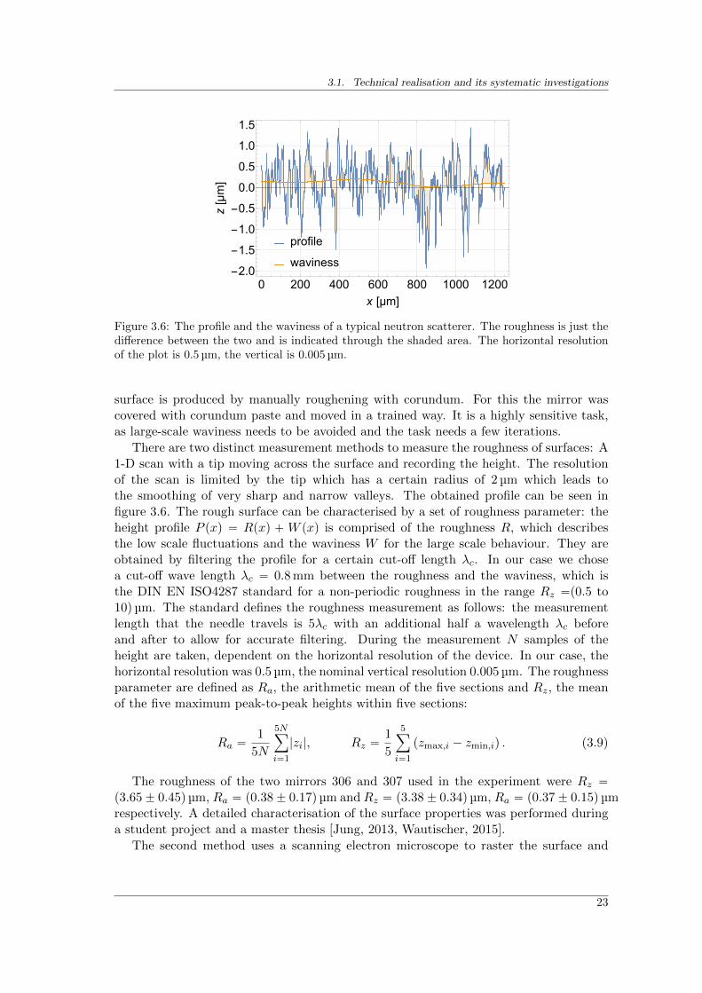
Figure 3.6: The profile and the waviness of a typical neutron scatterer. The roughness is just thedifference between the two and is indicated through the shaded area. The horizontal resolutionof the plot is 0.5 µm, the vertical is 0.005 µm.
surface is produced by manually roughening with corundum. For this the mirror wascovered with corundum paste and moved in a trained way. It is a highly sensitive task,as large-scale waviness needs to be avoided and the task needs a few iterations.
There are two distinct measurement methods to measure the roughness of surfaces: A1-D scan with a tip moving across the surface and recording the height. The resolutionof the scan is limited by the tip which has a certain radius of 2 µm which leads tothe smoothing of very sharp and narrow valleys. The obtained profile can be seen infigure 3.6. The rough surface can be characterised by a set of roughness parameter: theheight profile P pxq “ Rpxq `W pxq is comprised of the roughness R, which describesthe low scale fluctuations and the waviness W for the large scale behaviour. They areobtained by filtering the profile for a certain cut-off length λc. In our case we chosea cut-off wave length λc “ 0.8 mm between the roughness and the waviness, which isthe DIN EN ISO4287 standard for a non-periodic roughness in the range Rz “p0.5 to10q µm. The standard defines the roughness measurement as follows: the measurementlength that the needle travels is 5λc with an additional half a wavelength λc beforeand after to allow for accurate filtering. During the measurement N samples of theheight are taken, dependent on the horizontal resolution of the device. In our case, thehorizontal resolution was 0.5 µm, the nominal vertical resolution 0.005 µm. The roughnessparameter are defined as Ra, the arithmetic mean of the five sections and Rz, the meanof the five maximum peak-to-peak heights within five sections:
Ra “1
5N
5Nÿ
i“1
|zi|, Rz “1
5
5ÿ
i“1
pzmax,i ´ zmin,iq . (3.9)
The roughness of the two mirrors 306 and 307 used in the experiment were Rz “p3.65˘ 0.45q µm, Ra “ p0.38˘ 0.17q µm andRz “ p3.38˘ 0.34q µm, Ra “ p0.37˘ 0.15q µmrespectively. A detailed characterisation of the surface properties was performed duringa student project and a master thesis [Jung, 2013, Wautischer, 2015].
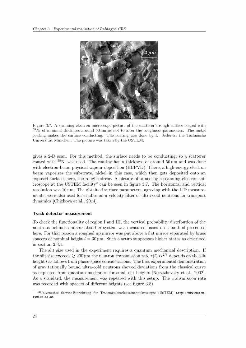
The second method uses a scanning electron microscope to raster the surface and
23
Chapter 3. Experimental realisation of Rabi-type GRS
Figure 3.7: A scanning electron microscope picture of the scatterer’s rough surface coated with58Ni of minimal thickness around 50 nm as not to alter the roughness parameters. The nickelcoating makes the surface conducting. The coating was done by D. Seiler at the TechnischeUniversitat Munchen. The picture was taken by the USTEM.
gives a 2-D scan. For this method, the surface needs to be conducting, so a scatterercoated with 58Ni was used. The coating has a thickness of around 50 nm and was donewith electron-beam physical vapour deposition (EBPVD). There, a high-energy electronbeam vaporizes the substrate, nickel in this case, which then gets deposited onto anexposed surface, here, the rough mirror. A picture obtained by a scanning electron mi-croscope at the USTEM facility2 can be seen in figure 3.7. The horizontal and verticalresolution was 10 nm. The obtained surface parameters, agreeing with the 1-D measure-ments, were also used for studies on a velocity filter of ultra-cold neutrons for transportdynamics [Chizhova et al., 2014].
Track detector measurement
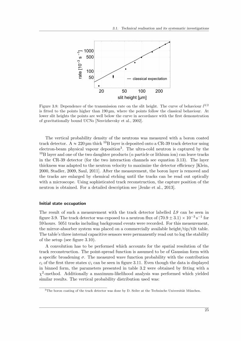
To check the functionality of region I and III, the vertical probability distribution of theneutrons behind a mirror-absorber system was measured based on a method presentedhere. For that reason a roughed up mirror was put above a flat mirror separated by brassspacers of nominal height l “ 30 µm. Such a setup suppresses higher states as describedin section 2.3.1.
The slit size used in the experiment requires a quantum mechanical description. Ifthe slit size exceeds Á 200 µm the neutron transmission rate rplq9l23 depends on the slitheight l as follows from phase-space considerations. The first experimental demonstrationof gravitationally bound ultra-cold neutrons showed deviations from the classical curveas expected from quantum mechanics for small slit heights [Nesvizhevsky et al., 2002].As a standard, the measurement was repeated with this setup. The transmission ratewas recorded with spacers of different heights (see figure 3.8).
2Universitare Service-Einrichtung fur Transmissionselektronenmikroskopie (USTEM) http://www.ustem.
tuwien.ac.at
24
3.1. Technical realisation and its systematic investigations
classical expectation
20 50 100 200
50100
5001000
slit height [µm]
rate
[10-3s
-1]
Figure 3.8: Dependence of the transmission rate on the slit height. The curve of behaviour l32
is fitted to the points higher than 190 µm, where the points follow the classical behaviour. Atlower slit heights the points are well below the curve in accordance with the first demonstrationof gravitationally bound UCNs [Nesvizhevsky et al., 2002].
The vertical probability density of the neutrons was measured with a boron coatedtrack detector. A « 220 µm thick 10B layer is deposited onto a CR-39 track detector usingelectron-beam physical vapour deposition3. The ultra-cold neutron is captured by the10B layer and one of the two daughter products (α particle or lithium ion) can leave tracksin the CR-39 detector (for the two interaction channels see equation 3.13). The layerthickness was adapted to the neutron velocity to maximize the detector efficiency [Klein,2000, Stadler, 2009, Saul, 2011]. After the measurement, the boron layer is removed andthe tracks are enlarged by chemical etching until the tracks can be read out opticallywith a microscope. Using sophisticated track reconstruction, the capture position of theneutron is obtained. For a detailed description see [Jenke et al., 2013].
Initial state occupation
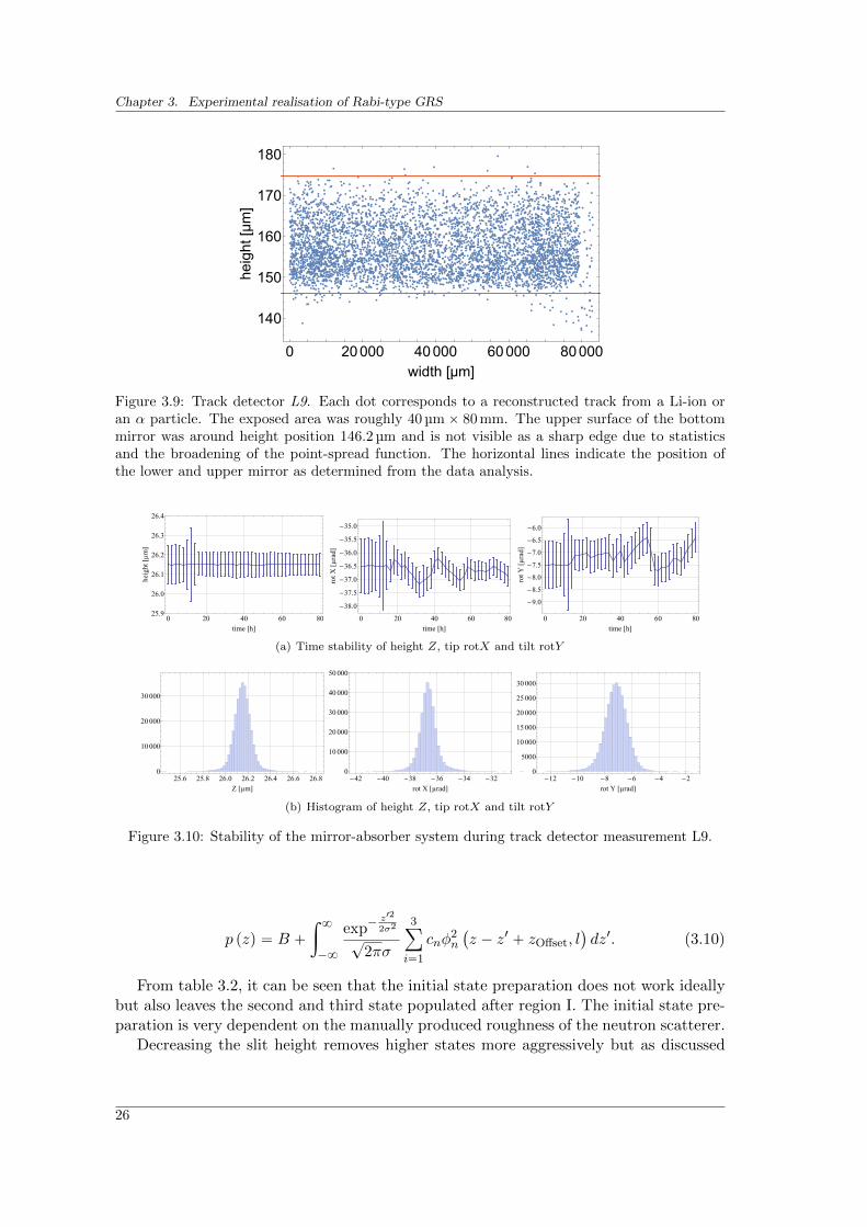
The result of such a measurement with the track detector labelled L9 can be seen infigure 3.9. The track detector was exposed to a neutron flux of p70.9˘ 3.1q ˆ 10´3 s´1 for59 hours. 5051 tracks including background events were recorded. For this measurement,the mirror-absorber system was placed on a commercially available height/tip/tilt table.The table’s three internal capacitive sensors were permanently read out to log the stabilityof the setup (see figure 3.10).
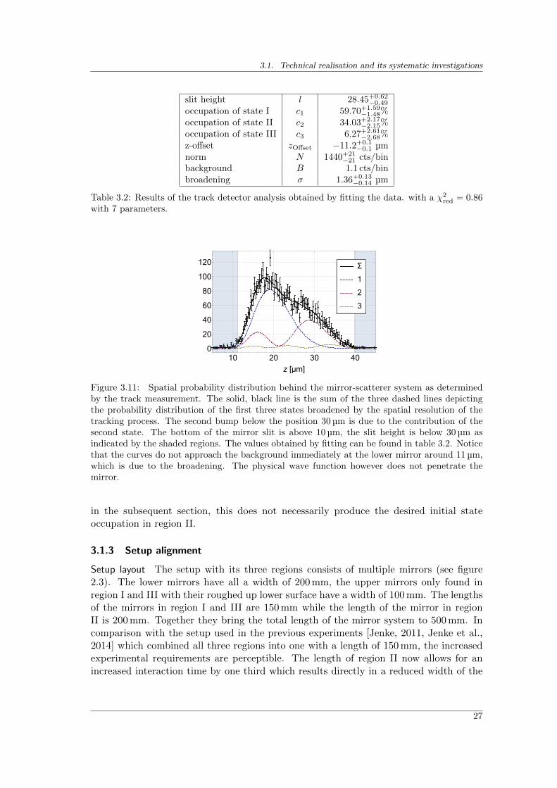
A convolution has to be performed which accounts for the spatial resolution of thetrack reconstruction. The point-spread function is assumed to be of Gaussian form witha specific broadening σ. The measured wave function probability with the contributionci of the first three states ψi can be seen in figure 3.11. Even though the data is displayedin binned form, the parameters presented in table 3.2 were obtained by fitting with aχ2-method. Additionally a maximum-likelihood analysis was performed which yieldedsimilar results. The vertical probability distribution used was:
3The boron coating of the track detector was done by D. Seiler at the Technische Universitat Munchen.
25
Chapter 3. Experimental realisation of Rabi-type GRS
0 20000 40000 60000 80000
140
150
160
170
180
width [µm]
height
[µm]
Figure 3.9: Track detector L9. Each dot corresponds to a reconstructed track from a Li-ion oran α particle. The exposed area was roughly 40 µm ˆ 80 mm. The upper surface of the bottommirror was around height position 146.2 µm and is not visible as a sharp edge due to statisticsand the broadening of the point-spread function. The horizontal lines indicate the position ofthe lower and upper mirror as determined from the data analysis.
0 20 40 60 8025.9
26.0
26.1
26.2
26.3
26.4
time @hD
heig
ht@µm
D
0 20 40 60 80
-38.0
-37.5
-37.0
-36.5
-36.0
-35.5
-35.0
time @hD
rotX
@µrad
D
0 20 40 60 80
-9.0
-8.5
-8.0
-7.5
-7.0
-6.5
-6.0
time @hD
rotY
@µrad
D
(a) Time stability of height Z, tip rotX and tilt rotY
25.6 25.8 26.0 26.2 26.4 26.6 26.80
10 000
20 000
30 000
Z @µmD-42 -40 -38 -36 -34 -32
0
10 000
20 000
30 000
40 000
50 000
rot X @µradD-12 -10 -8 -6 -4 -2
0
5000
10 000
15 000
20 000
25 000
30 000
rot Y @µradD
(b) Histogram of height Z, tip rotX and tilt rotY
Figure 3.10: Stability of the mirror-absorber system during track detector measurement L9.
p pzq “ B `
ż 8
´8
exp´z12
2σ2
?2πσ
3ÿ
i“1
cnφ2n
`
z ´ z1 ` zOffset, l˘
dz1. (3.10)
From table 3.2, it can be seen that the initial state preparation does not work ideallybut also leaves the second and third state populated after region I. The initial state pre-paration is very dependent on the manually produced roughness of the neutron scatterer.
Decreasing the slit height removes higher states more aggressively but as discussed
26
3.1. Technical realisation and its systematic investigations
slit height l 28.45`0.62´0.49
occupation of state I c1 59.70`1.59´1.48%
occupation of state II c2 34.03`2.17´2.15%
occupation of state III c3 6.27`2.61´2.68%
z-offset zOffset ´11.2`0.1´0.1 µm
norm N 1440`21´21 cts/bin
background B 1.1 cts/binbroadening σ 1.36`0.13
´0.14 µm
Table 3.2: Results of the track detector analysis obtained by fitting the data. with a χ2red “ 0.86
with 7 parameters.
Σ
1
2
3
10 20 30 400
20
40
60
80
100
120
z [µm]
Figure 3.11: Spatial probability distribution behind the mirror-scatterer system as determinedby the track measurement. The solid, black line is the sum of the three dashed lines depictingthe probability distribution of the first three states broadened by the spatial resolution of thetracking process. The second bump below the position 30 µm is due to the contribution of thesecond state. The bottom of the mirror slit is above 10 µm, the slit height is below 30 µm asindicated by the shaded regions. The values obtained by fitting can be found in table 3.2. Noticethat the curves do not approach the background immediately at the lower mirror around 11 µm,which is due to the broadening. The physical wave function however does not penetrate themirror.
in the subsequent section, this does not necessarily produce the desired initial stateoccupation in region II.
3.1.3 Setup alignment
Setup layout The setup with its three regions consists of multiple mirrors (see figure2.3). The lower mirrors have all a width of 200 mm, the upper mirrors only found inregion I and III with their roughed up lower surface have a width of 100 mm. The lengthsof the mirrors in region I and III are 150 mm while the length of the mirror in regionII is 200 mm. Together they bring the total length of the mirror system to 500 mm. Incomparison with the setup used in the previous experiments [Jenke, 2011, Jenke et al.,2014] which combined all three regions into one with a length of 150 mm, the increasedexperimental requirements are perceptible. The length of region II now allows for anincreased interaction time by one third which results directly in a reduced width of the
27
Chapter 3. Experimental realisation of Rabi-type GRS
Physik Instrumente (PI) GmbH & Co. KG_Auf der Römerstrasse 1_76228 Karlsruhe, Germany Telefon +49 721 4846-0, Fax +49 721 4846-1019, E-mail [email protected], www.pi.ws
Sensorlage P-518.TCD:
Sensor 1
Sensor 2
Sensor 3
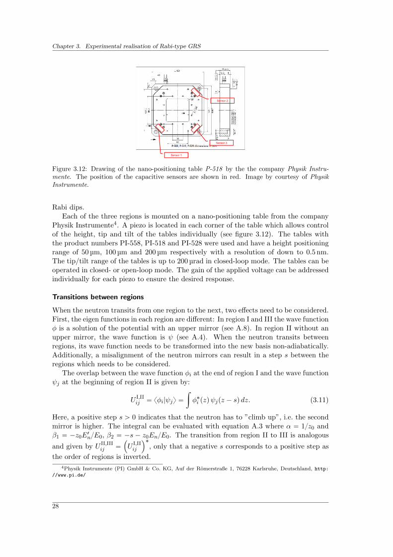
Figure 3.12: Drawing of the nano-positioning table P-518 by the the company Physik Instru-mente. The position of the capacitive sensors are shown in red. Image by courtesy of PhysikInstrumente.
Rabi dips.Each of the three regions is mounted on a nano-positioning table from the company
Physik Instrumente4. A piezo is located in each corner of the table which allows controlof the height, tip and tilt of the tables individually (see figure 3.12). The tables withthe product numbers PI-558, PI-518 and PI-528 were used and have a height positioningrange of 50 µm, 100 µm and 200 µm respectively with a resolution of down to 0.5 nm.The tip/tilt range of the tables is up to 200 µrad in closed-loop mode. The tables can beoperated in closed- or open-loop mode. The gain of the applied voltage can be addressedindividually for each piezo to ensure the desired response.
Transitions between regions
When the neutron transits from one region to the next, two effects need to be considered.First, the eigen functions in each region are different: In region I and III the wave functionφ is a solution of the potential with an upper mirror (see A.8). In region II without anupper mirror, the wave function is ψ (see A.4). When the neutron transits betweenregions, its wave function needs to be transformed into the new basis non-adiabatically.Additionally, a misalignment of the neutron mirrors can result in a step s between theregions which needs to be considered.
The overlap between the wave function φi at the end of region I and the wave functionψj at the beginning of region II is given by:
U I,IIij “ xφi|ψjy “
ż
φ˚i pzqψjpz ´ sq dz. (3.11)
Here, a positive step s ą 0 indicates that the neutron has to ”climb up”, i.e. the secondmirror is higher. The integral can be evaluated with equation A.3 where α “ 1z0 andβ1 “ ´z0E
1nE0, β2 “ ´s ´ z0EnE0. The transition from region II to III is analogous
and given by U II,IIIij “
´
U I,IIij
¯˚
, only that a negative s corresponds to a positive step as
the order of regions is inverted.
4Physik Instrumente (PI) GmbH & Co. KG, Auf der Romerstraße 1, 76228 Karlsruhe, Deutschland, http:
//www.pi.de/
28
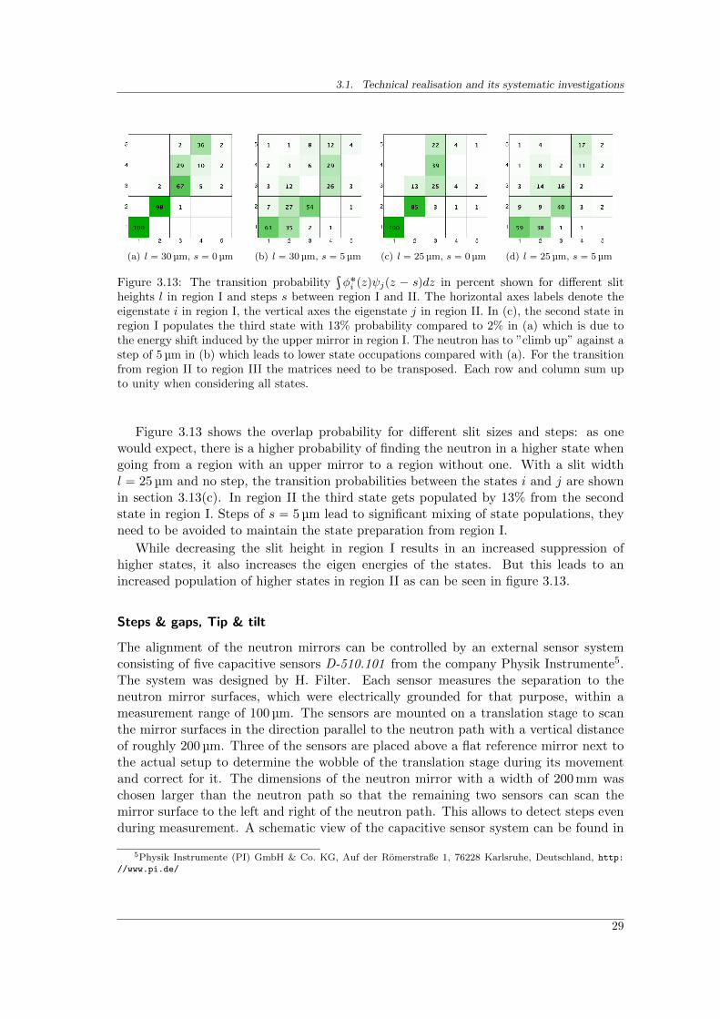
3.1. Technical realisation and its systematic investigations
(a) l “ 30 µm, s “ 0 µm (b) l “ 30 µm, s “ 5 µm (c) l “ 25 µm, s “ 0 µm (d) l “ 25 µm, s “ 5 µm
Figure 3.13: The transition probabilityş
φ˚i pzqψjpz ´ sqdz in percent shown for different slitheights l in region I and steps s between region I and II. The horizontal axes labels denote theeigenstate i in region I, the vertical axes the eigenstate j in region II. In (c), the second state inregion I populates the third state with 13% probability compared to 2% in (a) which is due tothe energy shift induced by the upper mirror in region I. The neutron has to ”climb up” against astep of 5 µm in (b) which leads to lower state occupations compared with (a). For the transitionfrom region II to region III the matrices need to be transposed. Each row and column sum upto unity when considering all states.
Figure 3.13 shows the overlap probability for different slit sizes and steps: as onewould expect, there is a higher probability of finding the neutron in a higher state whengoing from a region with an upper mirror to a region without one. With a slit widthl “ 25 µm and no step, the transition probabilities between the states i and j are shownin section 3.13(c). In region II the third state gets populated by 13% from the secondstate in region I. Steps of s “ 5 µm lead to significant mixing of state populations, theyneed to be avoided to maintain the state preparation from region I.
While decreasing the slit height in region I results in an increased suppression ofhigher states, it also increases the eigen energies of the states. But this leads to anincreased population of higher states in region II as can be seen in figure 3.13.
Steps & gaps, Tip & tilt
The alignment of the neutron mirrors can be controlled by an external sensor systemconsisting of five capacitive sensors D-510.101 from the company Physik Instrumente5.The system was designed by H. Filter. Each sensor measures the separation to theneutron mirror surfaces, which were electrically grounded for that purpose, within ameasurement range of 100 µm. The sensors are mounted on a translation stage to scanthe mirror surfaces in the direction parallel to the neutron path with a vertical distanceof roughly 200 µm. Three of the sensors are placed above a flat reference mirror next tothe actual setup to determine the wobble of the translation stage during its movementand correct for it. The dimensions of the neutron mirror with a width of 200 mm waschosen larger than the neutron path so that the remaining two sensors can scan themirror surface to the left and right of the neutron path. This allows to detect steps evenduring measurement. A schematic view of the capacitive sensor system can be found in
5Physik Instrumente (PI) GmbH & Co. KG, Auf der Romerstraße 1, 76228 Karlsruhe, Deutschland, http:
//www.pi.de/
29
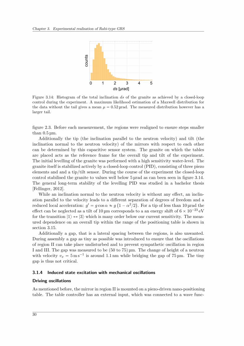
Chapter 3. Experimental realisation of Rabi-type GRS
0 1 2 3 4 5ds [µrad]
counts
Figure 3.14: Histogram of the total inclination ds of the granite as achieved by a closed-loopcontrol during the experiment. A maximum likelihood estimation of a Maxwell distribution forthe data without the tail gives a mean µ “ 0.52 µrad. The measured distribution however has alarger tail.
figure 2.3. Before each measurement, the regions were realigned to ensure steps smallerthan 0.5 µm.
Additionally the tip (the inclination parallel to the neutron velocity) and tilt (theinclination normal to the neutron velocity) of the mirrors with respect to each othercan be determined by this capacitive sensor system. The granite on which the tablesare placed acts as the reference frame for the overall tip and tilt of the experiment.The initial levelling of the granite was performed with a high sensitivity water-level. Thegranite itself is stabilized actively by a closed-loop control (PID), consisting of three piezoelements and and a tip/tilt sensor. During the course of the experiment the closed-loopcontrol stabilised the granite to values well below 5 µrad as can been seen in figure 3.14.The general long-term stability of the levelling PID was studied in a bachelor thesis[Fellinger, 2012].
While an inclination normal to the neutron velocity is without any effect, an inclin-ation parallel to the velocity leads to a different separation of degrees of freedom and areduced local acceleration: g1 “ g cosα « g
`
1´ α22˘
. For a tip of less than 10 µrad theeffect can be neglected as a tilt of 10 µm corresponds to a an energy shift of 6ˆ 10´23 eVfor the transition |1y Ø |3y which is many order below our current sensitivity. The meas-ured dependence on an overall tip within the range of the positioning table is shown insection 3.15.
Additionally a gap, that is a lateral spacing between the regions, is also unwanted.During assembly a gap as tiny as possible was introduced to ensure that the oscillationsof region II can take place undisturbed and to prevent sympathetic oscillation in regionI and III. The gap was measured to be p50 to 75q µm. The change of height of a neutronwith velocity vx “ 5 m s´1 is around 1.1 nm while bridging the gap of 75 µm. The tinygap is thus not critical.
3.1.4 Induced state excitation with mechanical oscillations
Driving oscillations
As mentioned before, the mirror in region II is mounted on a piezo-driven nano-positioningtable. The table controller has an external input, which was connected to a wave func-
30
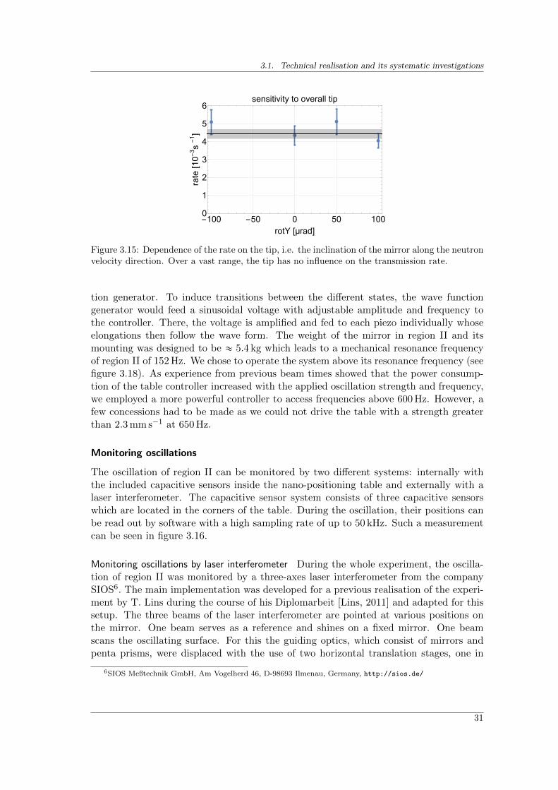
3.1. Technical realisation and its systematic investigations
-100 -50 0 50 1000
1
2
3
4
5
6
rotY [µrad]
rate
[10-3s
-1]
sensitivity to overall tip
Figure 3.15: Dependence of the rate on the tip, i.e. the inclination of the mirror along the neutronvelocity direction. Over a vast range, the tip has no influence on the transmission rate.
tion generator. To induce transitions between the different states, the wave functiongenerator would feed a sinusoidal voltage with adjustable amplitude and frequency tothe controller. There, the voltage is amplified and fed to each piezo individually whoseelongations then follow the wave form. The weight of the mirror in region II and itsmounting was designed to be « 5.4 kg which leads to a mechanical resonance frequencyof region II of 152 Hz. We chose to operate the system above its resonance frequency (seefigure 3.18). As experience from previous beam times showed that the power consump-tion of the table controller increased with the applied oscillation strength and frequency,we employed a more powerful controller to access frequencies above 600 Hz. However, afew concessions had to be made as we could not drive the table with a strength greaterthan 2.3 mm s´1 at 650 Hz.
Monitoring oscillations
The oscillation of region II can be monitored by two different systems: internally withthe included capacitive sensors inside the nano-positioning table and externally with alaser interferometer. The capacitive sensor system consists of three capacitive sensorswhich are located in the corners of the table. During the oscillation, their positions canbe read out by software with a high sampling rate of up to 50 kHz. Such a measurementcan be seen in figure 3.16.
Monitoring oscillations by laser interferometer During the whole experiment, the oscilla-tion of region II was monitored by a three-axes laser interferometer from the companySIOS6. The main implementation was developed for a previous realisation of the experi-ment by T. Lins during the course of his Diplomarbeit [Lins, 2011] and adapted for thissetup. The three beams of the laser interferometer are pointed at various positions onthe mirror. One beam serves as a reference and shines on a fixed mirror. One beamscans the oscillating surface. For this the guiding optics, which consist of mirrors andpenta prisms, were displaced with the use of two horizontal translation stages, one in
6SIOS Meßtechnik GmbH, Am Vogelherd 46, D-98693 Ilmenau, Germany, http://sios.de/
31
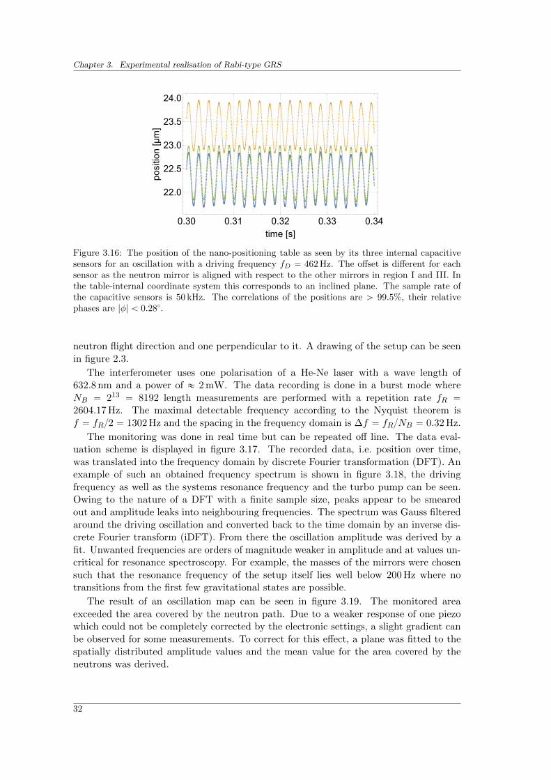
Chapter 3. Experimental realisation of Rabi-type GRS
0.30 0.31 0.32 0.33 0.34
22.0
22.5
23.0
23.5
24.0
time [s]
position[µm]
Figure 3.16: The position of the nano-positioning table as seen by its three internal capacitivesensors for an oscillation with a driving frequency fD “ 462 Hz. The offset is different for eachsensor as the neutron mirror is aligned with respect to the other mirrors in region I and III. Inthe table-internal coordinate system this corresponds to an inclined plane. The sample rate ofthe capacitive sensors is 50 kHz. The correlations of the positions are ą 99.5%, their relativephases are |φ| ă 0.280.
neutron flight direction and one perpendicular to it. A drawing of the setup can be seenin figure 2.3.
The interferometer uses one polarisation of a He-Ne laser with a wave length of632.8 nm and a power of « 2 mW. The data recording is done in a burst mode whereNB “ 213 “ 8192 length measurements are performed with a repetition rate fR “
2604.17 Hz. The maximal detectable frequency according to the Nyquist theorem isf “ fR2 “ 1302 Hz and the spacing in the frequency domain is ∆f “ fRNB “ 0.32 Hz.
The monitoring was done in real time but can be repeated off line. The data eval-uation scheme is displayed in figure 3.17. The recorded data, i.e. position over time,was translated into the frequency domain by discrete Fourier transformation (DFT). Anexample of such an obtained frequency spectrum is shown in figure 3.18, the drivingfrequency as well as the systems resonance frequency and the turbo pump can be seen.Owing to the nature of a DFT with a finite sample size, peaks appear to be smearedout and amplitude leaks into neighbouring frequencies. The spectrum was Gauss filteredaround the driving oscillation and converted back to the time domain by an inverse dis-crete Fourier transform (iDFT). From there the oscillation amplitude was derived by afit. Unwanted frequencies are orders of magnitude weaker in amplitude and at values un-critical for resonance spectroscopy. For example, the masses of the mirrors were chosensuch that the resonance frequency of the setup itself lies well below 200 Hz where notransitions from the first few gravitational states are possible.
The result of an oscillation map can be seen in figure 3.19. The monitored areaexceeded the area covered by the neutron path. Due to a weaker response of one piezowhich could not be completely corrected by the electronic settings, a slight gradient canbe observed for some measurements. To correct for this effect, a plane was fitted to thespatially distributed amplitude values and the mean value for the area covered by theneutrons was derived.
32
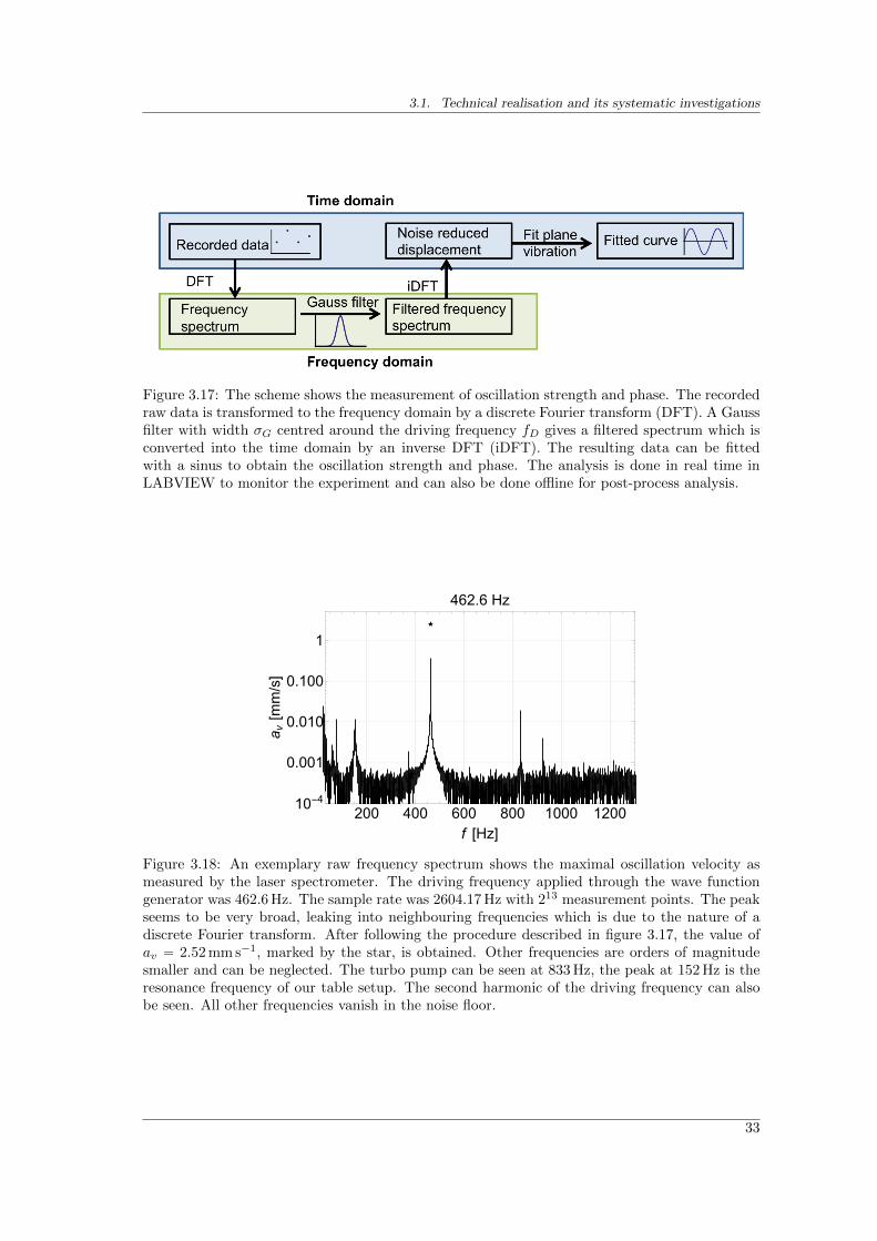
3.1. Technical realisation and its systematic investigations
Figure 3.17: The scheme shows the measurement of oscillation strength and phase. The recordedraw data is transformed to the frequency domain by a discrete Fourier transform (DFT). A Gaussfilter with width σG centred around the driving frequency fD gives a filtered spectrum which isconverted into the time domain by an inverse DFT (iDFT). The resulting data can be fittedwith a sinus to obtain the oscillation strength and phase. The analysis is done in real time inLABVIEW to monitor the experiment and can also be done offline for post-process analysis.
200 400 600 800 1000 120010-4
0.001
0.010
0.100
1
f [Hz]
a v[mm/s]
462.6 Hz
Figure 3.18: An exemplary raw frequency spectrum shows the maximal oscillation velocity asmeasured by the laser spectrometer. The driving frequency applied through the wave functiongenerator was 462.6 Hz. The sample rate was 2604.17 Hz with 213 measurement points. The peakseems to be very broad, leaking into neighbouring frequencies which is due to the nature of adiscrete Fourier transform. After following the procedure described in figure 3.17, the value ofav “ 2.52 mm s´1, marked by the star, is obtained. Other frequencies are orders of magnitudesmaller and can be neglected. The turbo pump can be seen at 833 Hz, the peak at 152 Hz is theresonance frequency of our table setup. The second harmonic of the driving frequency can alsobe seen. All other frequencies vanish in the noise floor.
33
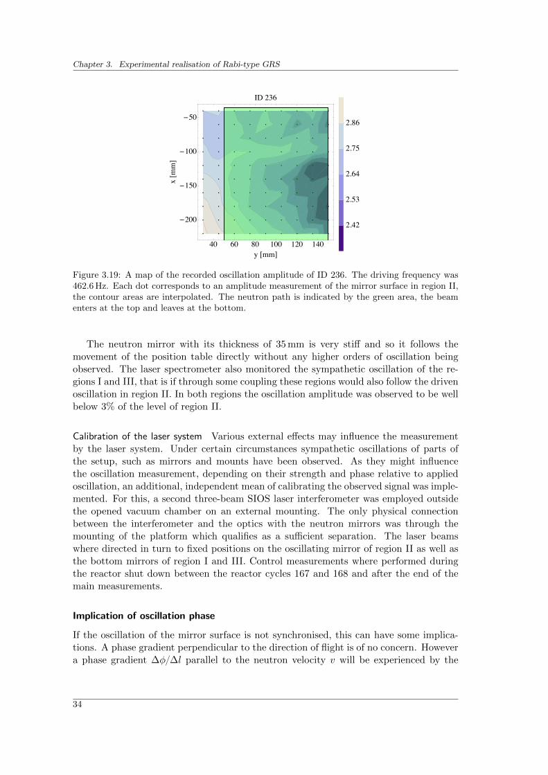
Chapter 3. Experimental realisation of Rabi-type GRS
40 60 80 100 120 140
-200
-150
-100
-50
y @mmD
x@mmD
ID 236
2.42
2.53
2.64
2.75
2.86
-6-4-20246
Figure 3.19: A map of the recorded oscillation amplitude of ID 236. The driving frequency was462.6 Hz. Each dot corresponds to an amplitude measurement of the mirror surface in region II,the contour areas are interpolated. The neutron path is indicated by the green area, the beamenters at the top and leaves at the bottom.
The neutron mirror with its thickness of 35 mm is very stiff and so it follows themovement of the position table directly without any higher orders of oscillation beingobserved. The laser spectrometer also monitored the sympathetic oscillation of the re-gions I and III, that is if through some coupling these regions would also follow the drivenoscillation in region II. In both regions the oscillation amplitude was observed to be wellbelow 3% of the level of region II.
Calibration of the laser system Various external effects may influence the measurementby the laser system. Under certain circumstances sympathetic oscillations of parts ofthe setup, such as mirrors and mounts have been observed. As they might influencethe oscillation measurement, depending on their strength and phase relative to appliedoscillation, an additional, independent mean of calibrating the observed signal was imple-mented. For this, a second three-beam SIOS laser interferometer was employed outsidethe opened vacuum chamber on an external mounting. The only physical connectionbetween the interferometer and the optics with the neutron mirrors was through themounting of the platform which qualifies as a sufficient separation. The laser beamswhere directed in turn to fixed positions on the oscillating mirror of region II as well asthe bottom mirrors of region I and III. Control measurements where performed duringthe reactor shut down between the reactor cycles 167 and 168 and after the end of themain measurements.
Implication of oscillation phase
If the oscillation of the mirror surface is not synchronised, this can have some implica-tions. A phase gradient perpendicular to the direction of flight is of no concern. Howevera phase gradient ∆φ∆l parallel to the neutron velocity v will be experienced by the
34
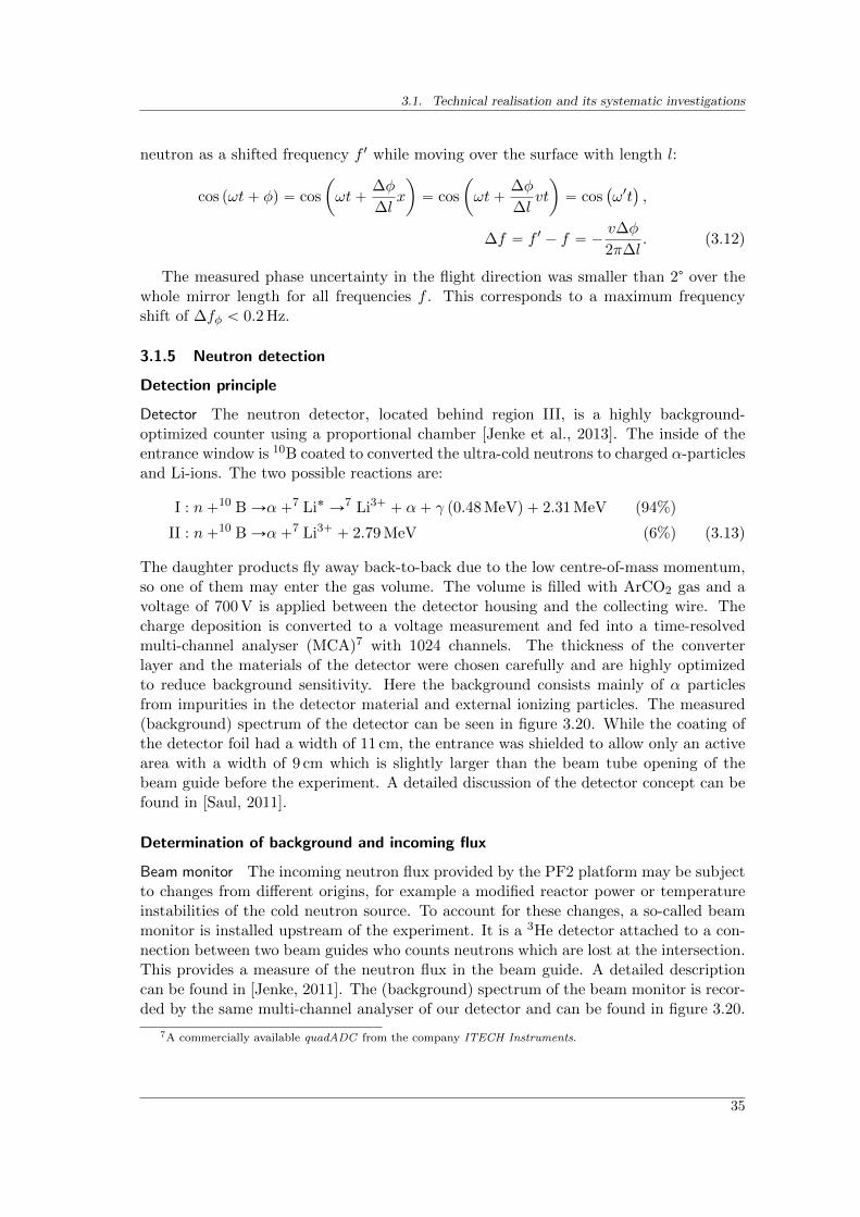
3.1. Technical realisation and its systematic investigations
neutron as a shifted frequency f 1 while moving over the surface with length l:
cos pωt` φq “ cos
ˆ
ωt`∆φ
∆lx
˙
“ cos
ˆ
ωt`∆φ
∆lvt
˙
“ cos`
ω1t˘
,
∆f “ f 1 ´ f “ ´v∆φ
2π∆l. (3.12)
The measured phase uncertainty in the flight direction was smaller than 2° over thewhole mirror length for all frequencies f . This corresponds to a maximum frequencyshift of ∆fφ ă 0.2 Hz.
3.1.5 Neutron detection
Detection principle
Detector The neutron detector, located behind region III, is a highly background-optimized counter using a proportional chamber [Jenke et al., 2013]. The inside of theentrance window is 10B coated to converted the ultra-cold neutrons to charged α-particlesand Li-ions. The two possible reactions are:
I : n`10 B Ñα`7 Li˚ Ñ7 Li3` ` α` γ p0.48 MeVq ` 2.31 MeV p94%q
II : n`10 B Ñα`7 Li3` ` 2.79 MeV p6%q (3.13)
The daughter products fly away back-to-back due to the low centre-of-mass momentum,so one of them may enter the gas volume. The volume is filled with ArCO2 gas and avoltage of 700 V is applied between the detector housing and the collecting wire. Thecharge deposition is converted to a voltage measurement and fed into a time-resolvedmulti-channel analyser (MCA)7 with 1024 channels. The thickness of the converterlayer and the materials of the detector were chosen carefully and are highly optimizedto reduce background sensitivity. Here the background consists mainly of α particlesfrom impurities in the detector material and external ionizing particles. The measured(background) spectrum of the detector can be seen in figure 3.20. While the coating ofthe detector foil had a width of 11 cm, the entrance was shielded to allow only an activearea with a width of 9 cm which is slightly larger than the beam tube opening of thebeam guide before the experiment. A detailed discussion of the detector concept can befound in [Saul, 2011].
Determination of background and incoming flux
Beam monitor The incoming neutron flux provided by the PF2 platform may be subjectto changes from different origins, for example a modified reactor power or temperatureinstabilities of the cold neutron source. To account for these changes, a so-called beammonitor is installed upstream of the experiment. It is a 3He detector attached to a con-nection between two beam guides who counts neutrons which are lost at the intersection.This provides a measure of the neutron flux in the beam guide. A detailed descriptioncan be found in [Jenke, 2011]. The (background) spectrum of the beam monitor is recor-ded by the same multi-channel analyser of our detector and can be found in figure 3.20.
7A commercially available quadADC from the company ITECH Instruments.
35
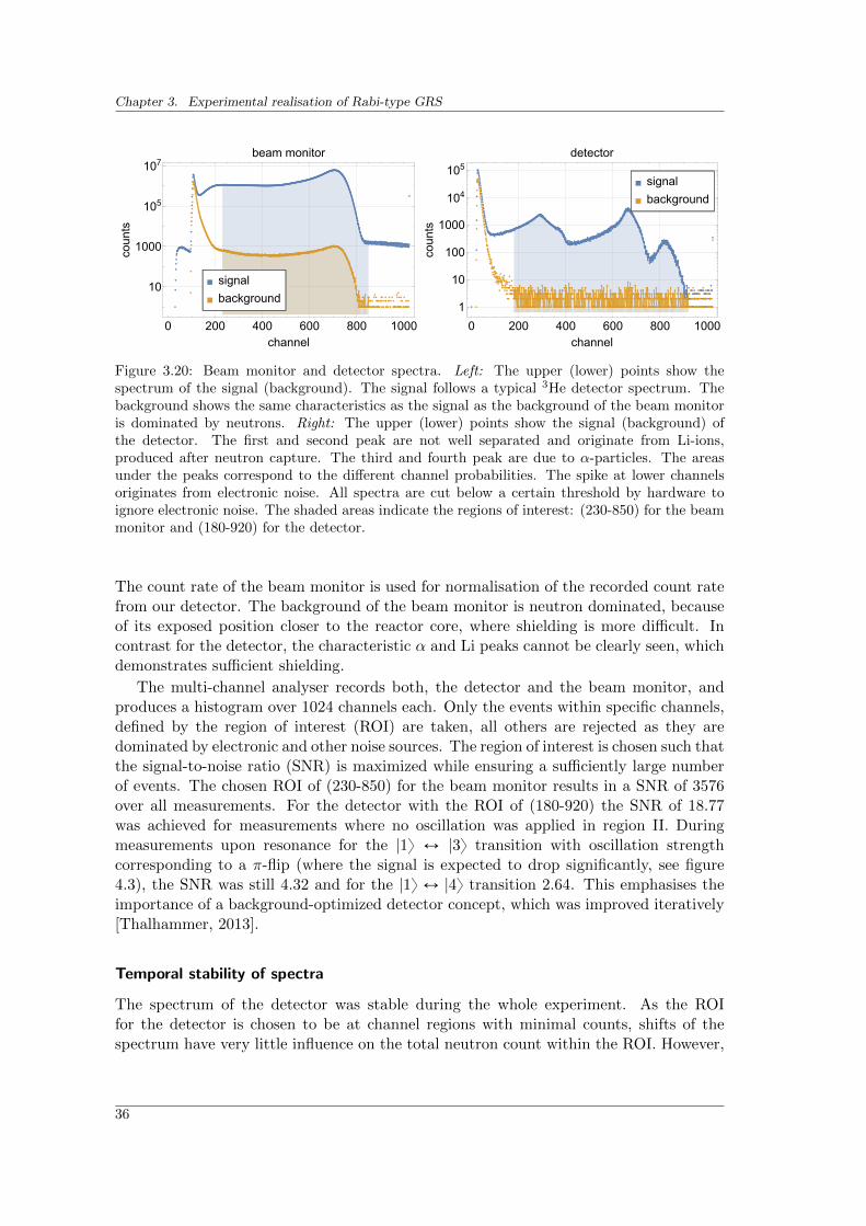
Chapter 3. Experimental realisation of Rabi-type GRS
0 200 400 600 800 1000
10
1000
105
107
channel
counts
beam monitor
signal
background
0 200 400 600 800 1000
1
10
100
1000
104
105
channel
counts
detector
signal
background
Figure 3.20: Beam monitor and detector spectra. Left: The upper (lower) points show thespectrum of the signal (background). The signal follows a typical 3He detector spectrum. Thebackground shows the same characteristics as the signal as the background of the beam monitoris dominated by neutrons. Right: The upper (lower) points show the signal (background) ofthe detector. The first and second peak are not well separated and originate from Li-ions,produced after neutron capture. The third and fourth peak are due to α-particles. The areasunder the peaks correspond to the different channel probabilities. The spike at lower channelsoriginates from electronic noise. All spectra are cut below a certain threshold by hardware toignore electronic noise. The shaded areas indicate the regions of interest: (230-850) for the beammonitor and (180-920) for the detector.
The count rate of the beam monitor is used for normalisation of the recorded count ratefrom our detector. The background of the beam monitor is neutron dominated, becauseof its exposed position closer to the reactor core, where shielding is more difficult. Incontrast for the detector, the characteristic α and Li peaks cannot be clearly seen, whichdemonstrates sufficient shielding.
The multi-channel analyser records both, the detector and the beam monitor, andproduces a histogram over 1024 channels each. Only the events within specific channels,defined by the region of interest (ROI) are taken, all others are rejected as they aredominated by electronic and other noise sources. The region of interest is chosen such thatthe signal-to-noise ratio (SNR) is maximized while ensuring a sufficiently large numberof events. The chosen ROI of (230-850) for the beam monitor results in a SNR of 3576over all measurements. For the detector with the ROI of (180-920) the SNR of 18.77was achieved for measurements where no oscillation was applied in region II. Duringmeasurements upon resonance for the |1y Ø |3y transition with oscillation strengthcorresponding to a π-flip (where the signal is expected to drop significantly, see figure4.3), the SNR was still 4.32 and for the |1y Ø |4y transition 2.64. This emphasises theimportance of a background-optimized detector concept, which was improved iteratively[Thalhammer, 2013].
Temporal stability of spectra
The spectrum of the detector was stable during the whole experiment. As the ROIfor the detector is chosen to be at channel regions with minimal counts, shifts of thespectrum have very little influence on the total neutron count within the ROI. However,
36
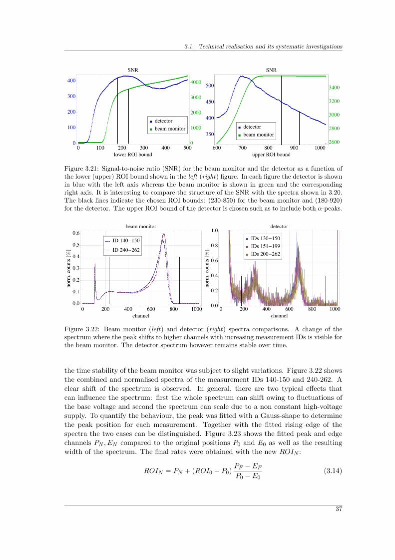
3.1. Technical realisation and its systematic investigations
0 100 200 300 400 5000
1000
2000
3000
4000
lower ROI bound
SNR
detectorbeam monitor
0
100
200
300
400
600 700 800 900 10002600
2800
3000
3200
3400
upper ROI bound
SNR
detectorbeam monitor350
400
450
500
Figure 3.21: Signal-to-noise ratio (SNR) for the beam monitor and the detector as a function ofthe lower (upper) ROI bound shown in the left (right) figure. In each figure the detector is shownin blue with the left axis whereas the beam monitor is shown in green and the correspondingright axis. It is interesting to compare the structure of the SNR with the spectra shown in 3.20.The black lines indicate the chosen ROI bounds: (230-850) for the beam monitor and (180-920)for the detector. The upper ROI bound of the detector is chosen such as to include both α-peaks.
0 200 400 600 800 10000.0
0.1
0.2
0.3
0.4
0.5
0.6
channel
norm.counts@%D
beam monitor
ID 140-150
ID 240-262
0 200 400 600 800 10000.0
0.2
0.4
0.6
0.8
1.0
channel
norm.counts@%D
detector
IDs 130-150IDs 151-199IDs 200-262
Figure 3.22: Beam monitor (left) and detector (right) spectra comparisons. A change of thespectrum where the peak shifts to higher channels with increasing measurement IDs is visible forthe beam monitor. The detector spectrum however remains stable over time.
the time stability of the beam monitor was subject to slight variations. Figure 3.22 showsthe combined and normalised spectra of the measurement IDs 140-150 and 240-262. Aclear shift of the spectrum is observed. In general, there are two typical effects thatcan influence the spectrum: first the whole spectrum can shift owing to fluctuations ofthe base voltage and second the spectrum can scale due to a non constant high-voltagesupply. To quantify the behaviour, the peak was fitted with a Gauss-shape to determinethe peak position for each measurement. Together with the fitted rising edge of thespectra the two cases can be distinguished. Figure 3.23 shows the fitted peak and edgechannels PN , EN compared to the original positions P0 and E0 as well as the resultingwidth of the spectrum. The final rates were obtained with the new ROIN :
ROIN “ PN ` pROI0 ´ P0qPF ´ EFP0 ´ E0
(3.14)
37
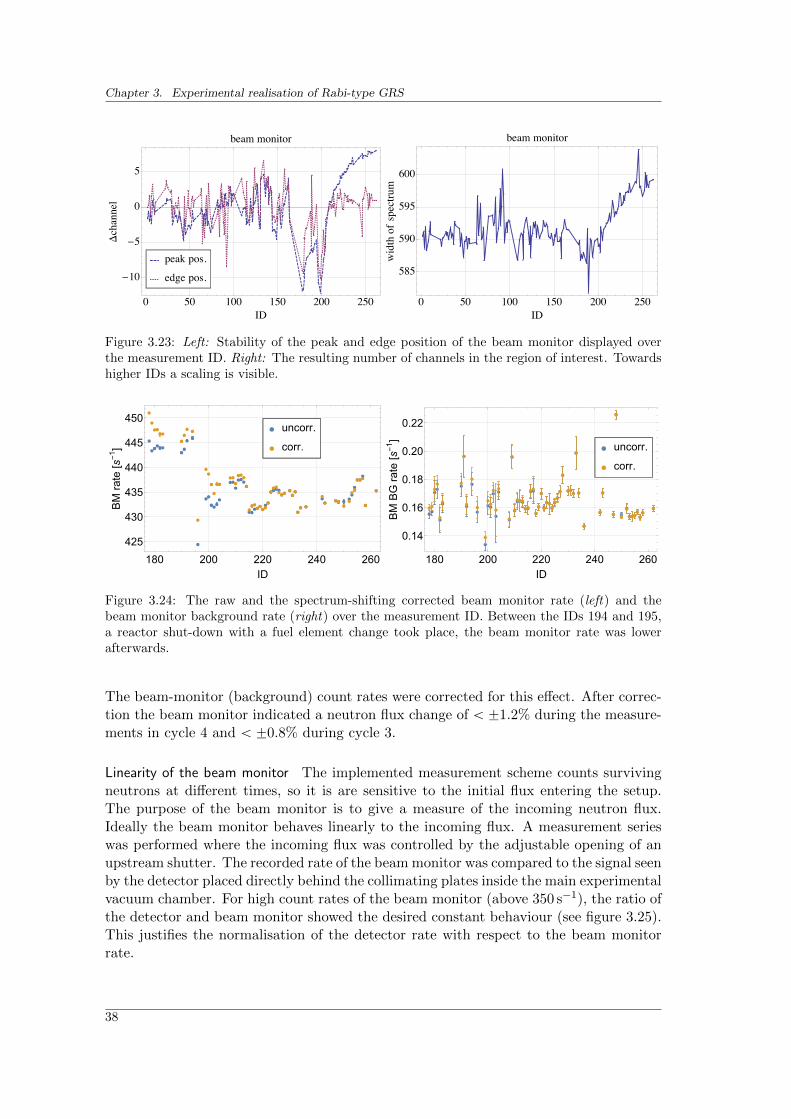
Chapter 3. Experimental realisation of Rabi-type GRS
0 50 100 150 200 250
-10
-5
0
5
ID
Dchannel
beam monitor
peak pos.
edge pos.
0 50 100 150 200 250
585
590
595
600
ID
widthofspectrum
beam monitor
Figure 3.23: Left: Stability of the peak and edge position of the beam monitor displayed overthe measurement ID. Right: The resulting number of channels in the region of interest. Towardshigher IDs a scaling is visible.
180 200 220 240 260
425
430
435
440
445
450
ID
BMrate
[s-1]
uncorr.
corr.
180 200 220 240 260
0.14
0.16
0.18
0.20
0.22
ID
BMBGrate
[s-1]
uncorr.
corr.
Figure 3.24: The raw and the spectrum-shifting corrected beam monitor rate (left) and thebeam monitor background rate (right) over the measurement ID. Between the IDs 194 and 195,a reactor shut-down with a fuel element change took place, the beam monitor rate was lowerafterwards.
The beam-monitor (background) count rates were corrected for this effect. After correc-tion the beam monitor indicated a neutron flux change of ă ˘1.2% during the measure-ments in cycle 4 and ă ˘0.8% during cycle 3.
Linearity of the beam monitor The implemented measurement scheme counts survivingneutrons at different times, so it is are sensitive to the initial flux entering the setup.The purpose of the beam monitor is to give a measure of the incoming neutron flux.Ideally the beam monitor behaves linearly to the incoming flux. A measurement serieswas performed where the incoming flux was controlled by the adjustable opening of anupstream shutter. The recorded rate of the beam monitor was compared to the signal seenby the detector placed directly behind the collimating plates inside the main experimentalvacuum chamber. For high count rates of the beam monitor (above 350 s´1), the ratio ofthe detector and beam monitor showed the desired constant behaviour (see figure 3.25).This justifies the normalisation of the detector rate with respect to the beam monitorrate.
38
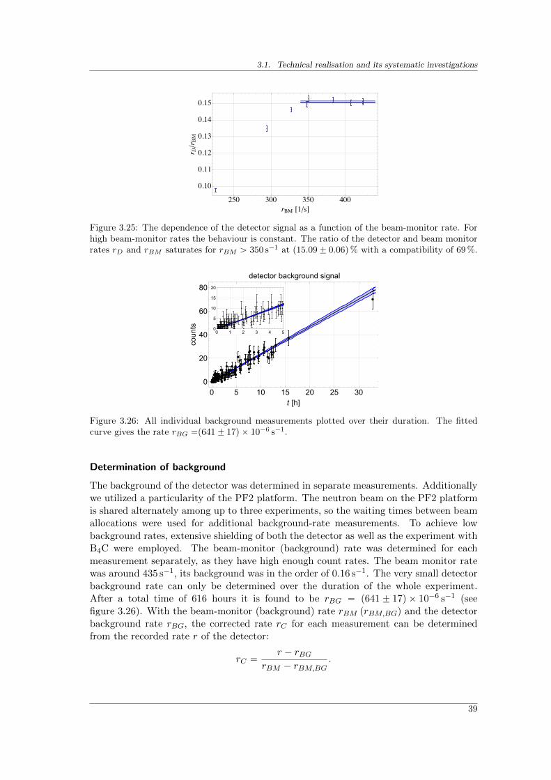
3.1. Technical realisation and its systematic investigations
250 300 350 400
0.10
0.11
0.12
0.13
0.14
0.15
rBM @1êsDr Dêr BM
Figure 3.25: The dependence of the detector signal as a function of the beam-monitor rate. Forhigh beam-monitor rates the behaviour is constant. The ratio of the detector and beam monitorrates rD and rBM saturates for rBM ą 350 s´1 at p15.09˘ 0.06q% with a compatibility of 69 %.
0 5 10 15 20 25 300
20
40
60
80
t [h]
counts
detector background signal
0 1 2 3 4 50
5
10
15
20
Figure 3.26: All individual background measurements plotted over their duration. The fittedcurve gives the rate rBG “p641˘ 17q ˆ 10´6 s´1.
Determination of background
The background of the detector was determined in separate measurements. Additionallywe utilized a particularity of the PF2 platform. The neutron beam on the PF2 platformis shared alternately among up to three experiments, so the waiting times between beamallocations were used for additional background-rate measurements. To achieve lowbackground rates, extensive shielding of both the detector as well as the experiment withB4C were employed. The beam-monitor (background) rate was determined for eachmeasurement separately, as they have high enough count rates. The beam monitor ratewas around 435 s´1, its background was in the order of 0.16 s´1. The very small detectorbackground rate can only be determined over the duration of the whole experiment.After a total time of 616 hours it is found to be rBG “ p641˘ 17q ˆ 10´6 s´1 (seefigure 3.26). With the beam-monitor (background) rate rBM prBM,BGq and the detectorbackground rate rBG, the corrected rate rC for each measurement can be determinedfrom the recorded rate r of the detector:
rC “r ´ rBG
rBM ´ rBM,BG.
39
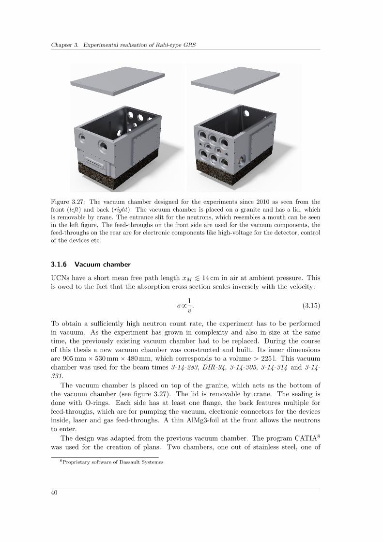
Chapter 3. Experimental realisation of Rabi-type GRS
Figure 3.27: The vacuum chamber designed for the experiments since 2010 as seen from thefront (left) and back (right). The vacuum chamber is placed on a granite and has a lid, whichis removable by crane. The entrance slit for the neutrons, which resembles a mouth can be seenin the left figure. The feed-throughs on the front side are used for the vacuum components, thefeed-throughs on the rear are for electronic components like high-voltage for the detector, controlof the devices etc.
3.1.6 Vacuum chamber
UCNs have a short mean free path length xM À 14 cm in air at ambient pressure. Thisis owed to the fact that the absorption cross section scales inversely with the velocity:
σ91
v. (3.15)
To obtain a sufficiently high neutron count rate, the experiment has to be performedin vacuum. As the experiment has grown in complexity and also in size at the sametime, the previously existing vacuum chamber had to be replaced. During the courseof this thesis a new vacuum chamber was constructed and built. Its inner dimensionsare 905 mm ˆ 530 mm ˆ 480 mm, which corresponds to a volume ą 225 l. This vacuumchamber was used for the beam times 3-14-283, DIR-94, 3-14-305, 3-14-314 and 3-14-331.
The vacuum chamber is placed on top of the granite, which acts as the bottom ofthe vacuum chamber (see figure 3.27). The lid is removable by crane. The sealing isdone with O-rings. Each side has at least one flange, the back features multiple forfeed-throughs, which are for pumping the vacuum, electronic connectors for the devicesinside, laser and gas feed-throughs. A thin AlMg3-foil at the front allows the neutronsto enter.
The design was adapted from the previous vacuum chamber. The program CATIA8
was used for the creation of plans. Two chambers, one out of stainless steel, one of
8Proprietary software of Dassault Systemes
40
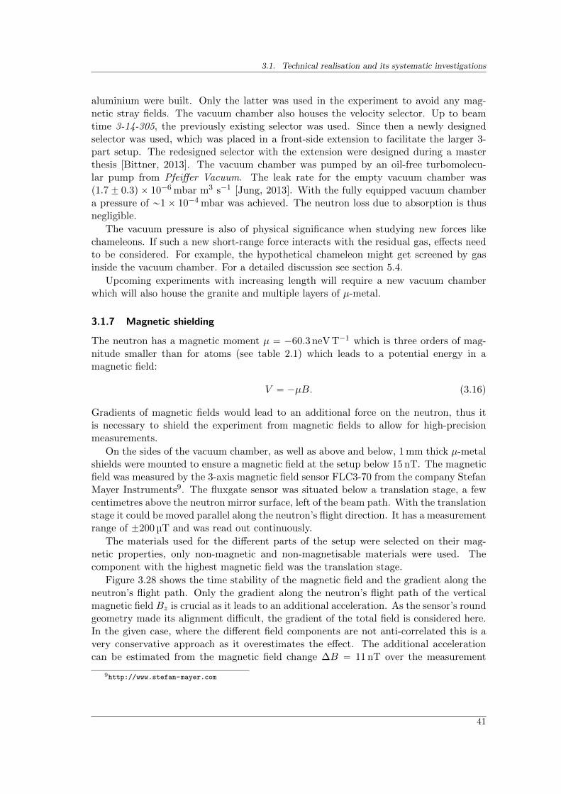
3.1. Technical realisation and its systematic investigations
aluminium were built. Only the latter was used in the experiment to avoid any mag-netic stray fields. The vacuum chamber also houses the velocity selector. Up to beamtime 3-14-305, the previously existing selector was used. Since then a newly designedselector was used, which was placed in a front-side extension to facilitate the larger 3-part setup. The redesigned selector with the extension were designed during a masterthesis [Bittner, 2013]. The vacuum chamber was pumped by an oil-free turbomolecu-lar pump from Pfeiffer Vacuum. The leak rate for the empty vacuum chamber wasp1.7˘ 0.3q ˆ 10´6 mbar m3 s´1 [Jung, 2013]. With the fully equipped vacuum chambera pressure of „1ˆ 10´4 mbar was achieved. The neutron loss due to absorption is thusnegligible.
The vacuum pressure is also of physical significance when studying new forces likechameleons. If such a new short-range force interacts with the residual gas, effects needto be considered. For example, the hypothetical chameleon might get screened by gasinside the vacuum chamber. For a detailed discussion see section 5.4.
Upcoming experiments with increasing length will require a new vacuum chamberwhich will also house the granite and multiple layers of µ-metal.
3.1.7 Magnetic shielding
The neutron has a magnetic moment µ “ ´60.3 neV T´1 which is three orders of mag-nitude smaller than for atoms (see table 2.1) which leads to a potential energy in amagnetic field:
V “ ´µB. (3.16)
Gradients of magnetic fields would lead to an additional force on the neutron, thus itis necessary to shield the experiment from magnetic fields to allow for high-precisionmeasurements.
On the sides of the vacuum chamber, as well as above and below, 1 mm thick µ-metalshields were mounted to ensure a magnetic field at the setup below 15 nT. The magneticfield was measured by the 3-axis magnetic field sensor FLC3-70 from the company StefanMayer Instruments9. The fluxgate sensor was situated below a translation stage, a fewcentimetres above the neutron mirror surface, left of the beam path. With the translationstage it could be moved parallel along the neutron’s flight direction. It has a measurementrange of ˘200 µT and was read out continuously.
The materials used for the different parts of the setup were selected on their mag-netic properties, only non-magnetic and non-magnetisable materials were used. Thecomponent with the highest magnetic field was the translation stage.
Figure 3.28 shows the time stability of the magnetic field and the gradient along theneutron’s flight path. Only the gradient along the neutron’s flight path of the verticalmagnetic field Bz is crucial as it leads to an additional acceleration. As the sensor’s roundgeometry made its alignment difficult, the gradient of the total field is considered here.In the given case, where the different field components are not anti-correlated this is avery conservative approach as it overestimates the effect. The additional accelerationcan be estimated from the magnetic field change ∆B “ 11 nT over the measurement
9http://www.stefan-mayer.com
41
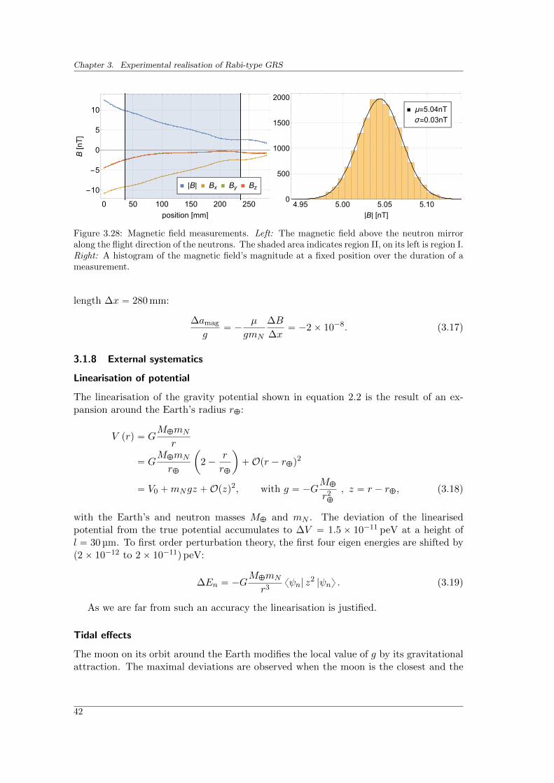
Chapter 3. Experimental realisation of Rabi-type GRS
|B| Bx By Bz
0 50 100 150 200 250
-10
-5
0
5
10
position [mm]
B[nT]
μ=5.04nT
σ=0.03nT
4.95 5.00 5.05 5.100
500
1000
1500
2000
|B| [nT]
Figure 3.28: Magnetic field measurements. Left: The magnetic field above the neutron mirroralong the flight direction of the neutrons. The shaded area indicates region II, on its left is region I.Right: A histogram of the magnetic field’s magnitude at a fixed position over the duration of ameasurement.
length ∆x “ 280 mm:
∆amag
g“ ´
µ
gmN
∆B
∆x“ ´2ˆ 10´8. (3.17)
3.1.8 External systematics
Linearisation of potential
The linearisation of the gravity potential shown in equation 2.2 is the result of an ex-pansion around the Earth’s radius rC:
V prq “ GMCmN
r
“ GMCmN
rC
ˆ
2´r
rC
˙
`Opr ´ rCq2
“ V0 `mNgz `Opzq2, with g “ ´GMC
r2C
, z “ r ´ rC, (3.18)
with the Earth’s and neutron masses MC and mN . The deviation of the linearisedpotential from the true potential accumulates to ∆V “ 1.5ˆ 10´11 peV at a height ofl “ 30 µm. To first order perturbation theory, the first four eigen energies are shifted byp2ˆ 10´12 to 2ˆ 10´11q peV:
∆En “ ´GMCmN
r3xψn| z
2 |ψny . (3.19)
As we are far from such an accuracy the linearisation is justified.
Tidal effects
The moon on its orbit around the Earth modifies the local value of g by its gravitationalattraction. The maximal deviations are observed when the moon is the closest and the
42
3.1. Technical realisation and its systematic investigations
furthest away respectively:
g1K “ ˘GMK
pdK ˘ rCq2 . (3.20)
This results in a relative changeg1
K
g “´3.5ˆ 10´6 to 3.3ˆ 10´6. Additionally the Earthrevolves in 27 days around the centre of mass which is located roughly 1680 km belowthe surface. The centrifugal force from this motion is directed away from the moon alongthe axis containing the mass centres of Earth and moon for every point on the Earth
and leads to an accelerationg2
K
g “ 3.4ˆ 10´6. This effect counteracts the gravitational
pull of the moon. The net effect of the moon gives gK
g “´9.9ˆ 10´8 to 1.2ˆ 10´7.
The sensitivity on the i-th state is given by
δEi “B
BgE0pgq AiZeropiq δg, (3.21)
with E0pgq “3
b
~2mNg22 from equation 2.6. The first four states have a sensitivity of
p2.1ˆ 10´7 to 6.1ˆ 10´7q peV.
The same is true for the sun on its diurnal path across the sky. Using equation 3.20with the sun mass M@ and distance d@ shows that the effect from the gravitational pull
is of orderg1
@
g “ ˘6.0ˆ 10´4 while the centrifugal force isg2
@
g “ ¯6.0ˆ 10´4 resulting in
a total effect g@
g “´5.6ˆ 10´8 to 4.7ˆ 10´8. This leads to a sensitivity of p9.7ˆ 10´8
to 2.8ˆ 10´7q peV for the first four states.
Coriolis force
The laboratory is no inertial frame as (among other things) the Earth rotates around itsaxis. Thus, in the laboratory reference frame pseudo forces like the Coriolis force FCor
appear. The Coriolis force couples the horizontal and vertical degrees of freedom. Itdepends on Earth’s angular velocity ωC and the flight direction of the neutron vN :
ÝÑF Cor “ ´2mN
ÝÑω C ˆÝÑv N . (3.22)
Equation 3.22 shows that only the component normal to the Earth’s rotation axis contrib-utes. The neutron, flying horizontally in the laboratory system with roughly v “ 8 m s´1
in Grenoble at a latitude of 45°, feels a maximal additional acceleration aCorg “ 8.4ˆ 10´5.
The energy of the first four states is thus shifted by p7.9ˆ 10´5 to 2.3ˆ 10´4q peV. Theeffect can be corrected for, a 2 degrees orientation uncertainty at a north-west alignmentof the experiment leads to a maximal uncertainty of 2ˆ 10´6 peV.
External mass distribution
Surrounding masses also modify the local acceleration felt by the neutron. For examplethe mirror on above the neutron in region I and III counteracts Earth’s gravity. Themirror has a density ρ “ 2.5 g cm´3 and let us assume the dimensions lx, ly, lz “ p200ˆ200 ˆ 35q mm. Treating the potential created from the mirror as a perturbation, the
43
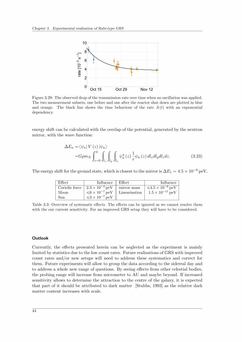
Chapter 3. Experimental realisation of Rabi-type GRS
Oct 15 Oct 29 Nov 120
2
4
6
8
10
rate
[10-3s-1]
Figure 3.29: The observed drop of the transmission rate over time when no oscillation was applied.The two measurement subsets, one before and one after the reactor shut down are plotted in blueand orange. The black line shows the time behaviour of the rate A ptq with an exponentialdependency.
energy shift can be calculated with the overlap of the potential, generated by the neutronmirror, with the wave function:
∆En “xψn|V pzq |ψny
“GρmN
ż 8
z“0
ż
lz
ż
ly
ż
lx
ψ˚n pzq1
rψn pzq dlxdlydlzdz. (3.23)
The energy shift for the ground state, which is closest to the mirror is ∆E1 “ 4.5ˆ 10´8 peV.
Effect Influence Effect InfluenceCoriolis force 2.3ˆ 10´4 peV mirror mass ď4.5ˆ 10´8 peVMoon ď6ˆ 10´7 peV Linearisation 1.5ˆ 10´11 peVSun ď3ˆ 10´7 peV
Table 3.3: Overview of systematic effects. The effects can be ignored as we cannot resolve themwith the our current sensitivity. For an improved GRS setup they will have to be considered.
Outlook
Currently, the effects presented herein can be neglected as the experiment is mainlylimited by statistics due to the low count rates. Future realisations of GRS with improvedcount rates and/or new setups will need to address these systematics and correct forthem. Future experiments will allow to group the data according to the sidereal day andto address a whole new range of questions. By seeing effects from other celestial bodies,the probing range will increase from micrometer to AU and maybe beyond. If increasedsensitivity allows to determine the attraction to the centre of the galaxy, it is expectedthat part of it should be attributed to dark matter [Stubbs, 1993] as the relative darkmatter content increases with scale.
44
3.1. Technical realisation and its systematic investigations
3.1.9 Null rate stability
The neutron flux was measured repeatedly when no oscillation was driven. Over the timeof the experiment, a degradation of this transmission rate was observed. The behaviourof transmission rate over time can be seen in figure 3.29. Small neutron flux variationsare normal at a neutron source like the ILL (see section 3.1.5), however for this significantchange, the definite origin is unknown. As the behaviour is not seen with a simplified1-part Rabi setup, it is likely that depositions like dust have accumulated on region IIover time as there is no protecting mirror above the surface. To test this hypothesis,the vacuum chamber was opened after the measurements and the surface of the mirrorin region II was carefully cleaned. An ensuing measurement without driven oscillationexhibited an increased count-rate. As no time for further investigations was available,no conclusive explanation for the behaviour can be given. The next generation of theexperiment will feature a protection against unwanted depositions.
The measurements extended over the two reactor cycles 167 and 168, in between wasa reactor halt for ten days. For the analysis we group the measurements into two subsets,according to the cycles.
To study the effect, various time dependent behaviours were tested on their compat-ibility with the data points where no oscillation was applied. The expected constantrate r0 was multiplied by a time dependent function Aptq to match the recorded rater “ Aptq r0. The compatibility of the following models can be seen in table 3.4.
Constant Choosing A ptq “ A0 as constant over time is not compatible with all measure-ments, it is labelled const. I in the results table 3.4. Even two individual constantrates for each of the two subsets are not compatible (labelled const. II ).
Linear drop The next to simplest approach is a linear time dependency A ptq “ A0´c0t.Still, the model does not explain the behaviour sufficiently.
Quadratic and higher orders The next polynomial order, a quadratic term is tested:A ptq “ A0 ` c0t
2. Still the compatibility is not high enough. Even increasing theorder of the polynomial up to four does not give satisfying results.
Exponential drop The model of exponential dampening of the rate uses the formA ptq “ c exp´kt`A0. This model describes the data best and is used in the dataevaluation in section 4.1. There the correction is applied to all data points. Themeasurements in the two subgroups can now be treated on the same footing, aseparation is not needed. The fitted curve is shown in figure 3.29.
Future realisation of GRS will include an additional setup protection against dust de-position from the top.
45
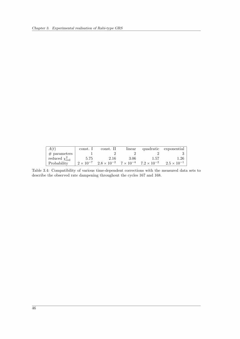
Chapter 3. Experimental realisation of Rabi-type GRS
Aptq const. I const. II linear quadratic exponential# parameters 1 2 2 2 3reduced χ2
red 5.75 2.16 3.06 1.57 1.26Probability 2ˆ 10´7 2.8ˆ 10´2 7ˆ 10´4 7.2ˆ 10´2 2.5ˆ 10´1
Table 3.4: Compatibility of various time-dependent corrections with the measured data sets todescribe the observed rate dampening throughout the cycles 167 and 168.
46
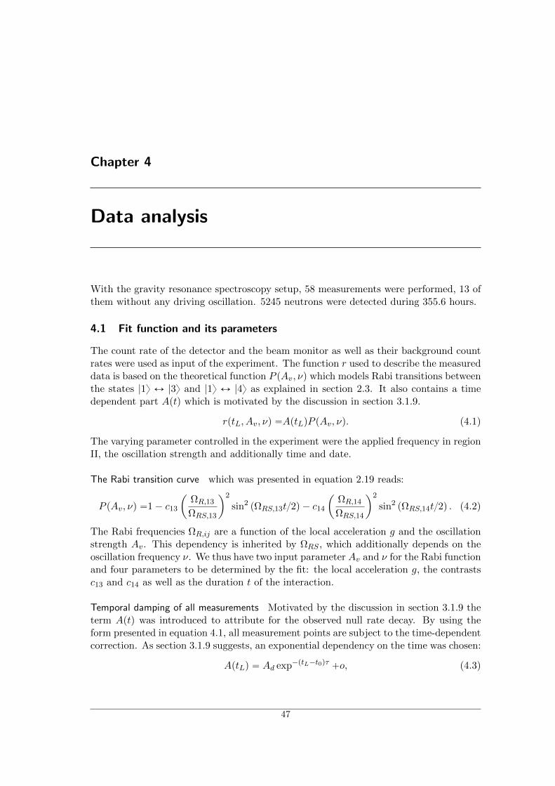
Chapter 4
Data analysis
With the gravity resonance spectroscopy setup, 58 measurements were performed, 13 ofthem without any driving oscillation. 5245 neutrons were detected during 355.6 hours.
4.1 Fit function and its parameters
The count rate of the detector and the beam monitor as well as their background countrates were used as input of the experiment. The function r used to describe the measureddata is based on the theoretical function P pAv, νq which models Rabi transitions betweenthe states |1y Ø |3y and |1y Ø |4y as explained in section 2.3. It also contains a timedependent part Aptq which is motivated by the discussion in section 3.1.9.
rptL, Av, νq “AptLqP pAv, νq. (4.1)
The varying parameter controlled in the experiment were the applied frequency in regionII, the oscillation strength and additionally time and date.
The Rabi transition curve which was presented in equation 2.19 reads:
P pAv, νq “1´ c13
ˆ
ΩR,13
ΩRS,13
˙2
sin2 pΩRS,13t2q ´ c14
ˆ
ΩR,14
ΩRS,14
˙2
sin2 pΩRS,14t2q . (4.2)
The Rabi frequencies ΩR,ij are a function of the local acceleration g and the oscillationstrength Av. This dependency is inherited by ΩRS , which additionally depends on theoscillation frequency ν. We thus have two input parameter Av and ν for the Rabi functionand four parameters to be determined by the fit: the local acceleration g, the contrastsc13 and c14 as well as the duration t of the interaction.
Temporal damping of all measurements Motivated by the discussion in section 3.1.9 theterm Aptq was introduced to attribute for the observed null rate decay. By using theform presented in equation 4.1, all measurement points are subject to the time-dependentcorrection. As section 3.1.9 suggests, an exponential dependency on the time was chosen:
AptLq “ Ad exp´ptL´t0qτ `o, (4.3)
47
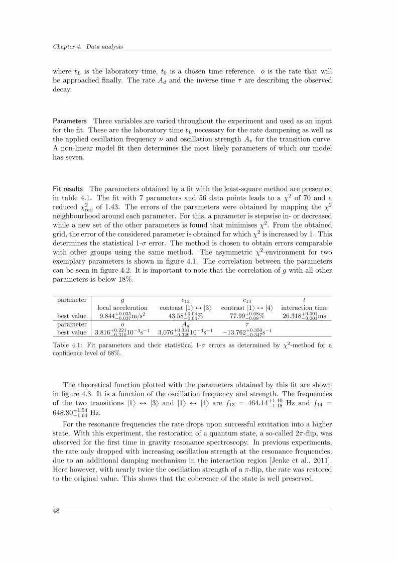
Chapter 4. Data analysis
where tL is the laboratory time, t0 is a chosen time reference. o is the rate that willbe approached finally. The rate Ad and the inverse time τ are describing the observeddecay.
Parameters Three variables are varied throughout the experiment and used as an inputfor the fit. These are the laboratory time tL necessary for the rate dampening as well asthe applied oscillation frequency ν and oscillation strength Av for the transition curve.A non-linear model fit then determines the most likely parameters of which our modelhas seven.
Fit results The parameters obtained by a fit with the least-square method are presentedin table 4.1. The fit with 7 parameters and 56 data points leads to a χ2 of 70 and areduced χ2
red of 1.43. The errors of the parameters were obtained by mapping the χ2
neighbourhood around each parameter. For this, a parameter is stepwise in- or decreasedwhile a new set of the other parameters is found that minimises χ2. From the obtainedgrid, the error of the considered parameter is obtained for which χ2 is increased by 1. Thisdetermines the statistical 1-σ error. The method is chosen to obtain errors comparablewith other groups using the same method. The asymmetric χ2-environment for twoexemplary parameters is shown in figure 4.1. The correlation between the parameterscan be seen in figure 4.2. It is important to note that the correlation of g with all otherparameters is below 18%.
parameter g c13 c14 tlocal acceleration contrast |1y Ø |3y contrast |1y Ø |4y interaction time
best value 9.844`0.035´0.037ms2 43.58`0.04
´0.04% 77.99`0.08´0.08% 26.318`0.001
´0.001msparameter o Ad τbest value 3.816`0.221
´0.31010´3s´1 3.076`0.331´0.32910´3s´1 ´13.762`0.350
´0.347s´1
Table 4.1: Fit parameters and their statistical 1-σ errors as determined by χ2-method for aconfidence level of 68%.
The theoretical function plotted with the parameters obtained by this fit are shownin figure 4.3. It is a function of the oscillation frequency and strength. The frequenciesof the two transitions |1y Ø |3y and |1y Ø |4y are f13 “ 464.14`1.10
´1.18 Hz and f14 “
648.80`1.54´1.64 Hz.
For the resonance frequencies the rate drops upon successful excitation into a higherstate. With this experiment, the restoration of a quantum state, a so-called 2π-flip, wasobserved for the first time in gravity resonance spectroscopy. In previous experiments,the rate only dropped with increasing oscillation strength at the resonance frequencies,due to an additional damping mechanism in the interaction region [Jenke et al., 2011].Here however, with nearly twice the oscillation strength of a π-flip, the rate was restoredto the original value. This shows that the coherence of the state is well preserved.
48
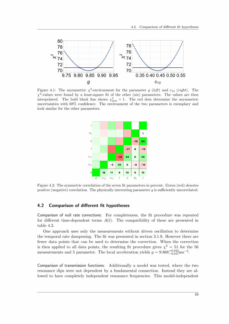
4.2. Comparison of different fit hypotheses
9.75 9.80 9.85 9.90 9.95707274767880
g
χ2
0.35 0.40 0.45 0.50 0.557072747678
c13
χ2
Figure 4.1: The asymmetric χ2-environment for the parameter g (left) and c13 (right). Theχ2-values were found by a least-square fit of the other (six) parameters. The values are theninterpolated. The bold black line shows χ2
min ` 1. The red dots determine the asymmetricuncertainties with 68% confidence. The environment of the two parameters is exemplary andlook similar for the other parameters.
Figure 4.2: The symmetric correlation of the seven fit parameters in percent. Green (red) denotespositive (negative) correlation. The physically interesting parameter g is sufficiently uncorrelated.
4.2 Comparison of different fit hypotheses
Comparison of null rate corrections: For completeness, the fit procedure was repeatedfor different time-dependent terms Aptq. The compatibility of these are presented intable 4.2.
One approach uses only the measurements without driven oscillation to determinethe temporal rate dampening. The fit was presented in section 3.1.9. However there arefewer data points that can be used to determine the correction. When the correctionis then applied to all data points, the resulting fit procedure gives χ2 “ 51 for the 56measurements and 5 parameter. The local acceleration yields g “ 9.868`0.042
´0.047ms´2.
Comparison of transmission functions: Additionally a model was tested, where the tworesonance dips were not dependent by a fundamental connection. Instead they are al-lowed to have completely independent resonance frequencies. This model-independent
49
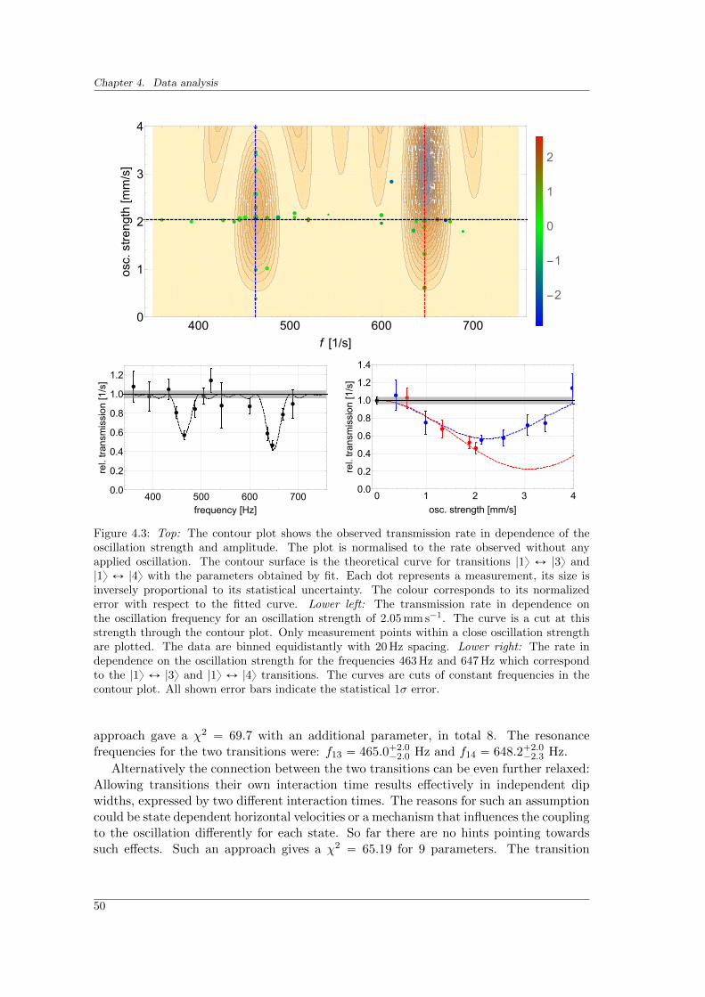
Chapter 4. Data analysis
400 500 600 7000
1
2
3
4
f [1/s]
osc.strength
[mm/s]
-2
-1
0
1
2
400 500 600 7000.0
0.2
0.4
0.6
0.8
1.0
1.2
frequency [Hz]
rel.transmission
[1/s]
0 1 2 3 40.0
0.2
0.4
0.6
0.8
1.0
1.2
1.4
osc. strength [mm/s]
rel.transmission
[1/s]
Figure 4.3: Top: The contour plot shows the observed transmission rate in dependence of theoscillation strength and amplitude. The plot is normalised to the rate observed without anyapplied oscillation. The contour surface is the theoretical curve for transitions |1y Ø |3y and|1y Ø |4y with the parameters obtained by fit. Each dot represents a measurement, its size isinversely proportional to its statistical uncertainty. The colour corresponds to its normalizederror with respect to the fitted curve. Lower left: The transmission rate in dependence onthe oscillation frequency for an oscillation strength of 2.05 mm s´1. The curve is a cut at thisstrength through the contour plot. Only measurement points within a close oscillation strengthare plotted. The data are binned equidistantly with 20 Hz spacing. Lower right: The rate independence on the oscillation strength for the frequencies 463 Hz and 647 Hz which correspondto the |1y Ø |3y and |1y Ø |4y transitions. The curves are cuts of constant frequencies in thecontour plot. All shown error bars indicate the statistical 1σ error.
approach gave a χ2 “ 69.7 with an additional parameter, in total 8. The resonancefrequencies for the two transitions were: f13 “ 465.0`2.0
´2.0 Hz and f14 “ 648.2`2.0´2.3 Hz.
Alternatively the connection between the two transitions can be even further relaxed:Allowing transitions their own interaction time results effectively in independent dipwidths, expressed by two different interaction times. The reasons for such an assumptioncould be state dependent horizontal velocities or a mechanism that influences the couplingto the oscillation differently for each state. So far there are no hints pointing towardssuch effects. Such an approach gives a χ2 “ 65.19 for 9 parameters. The transition
50
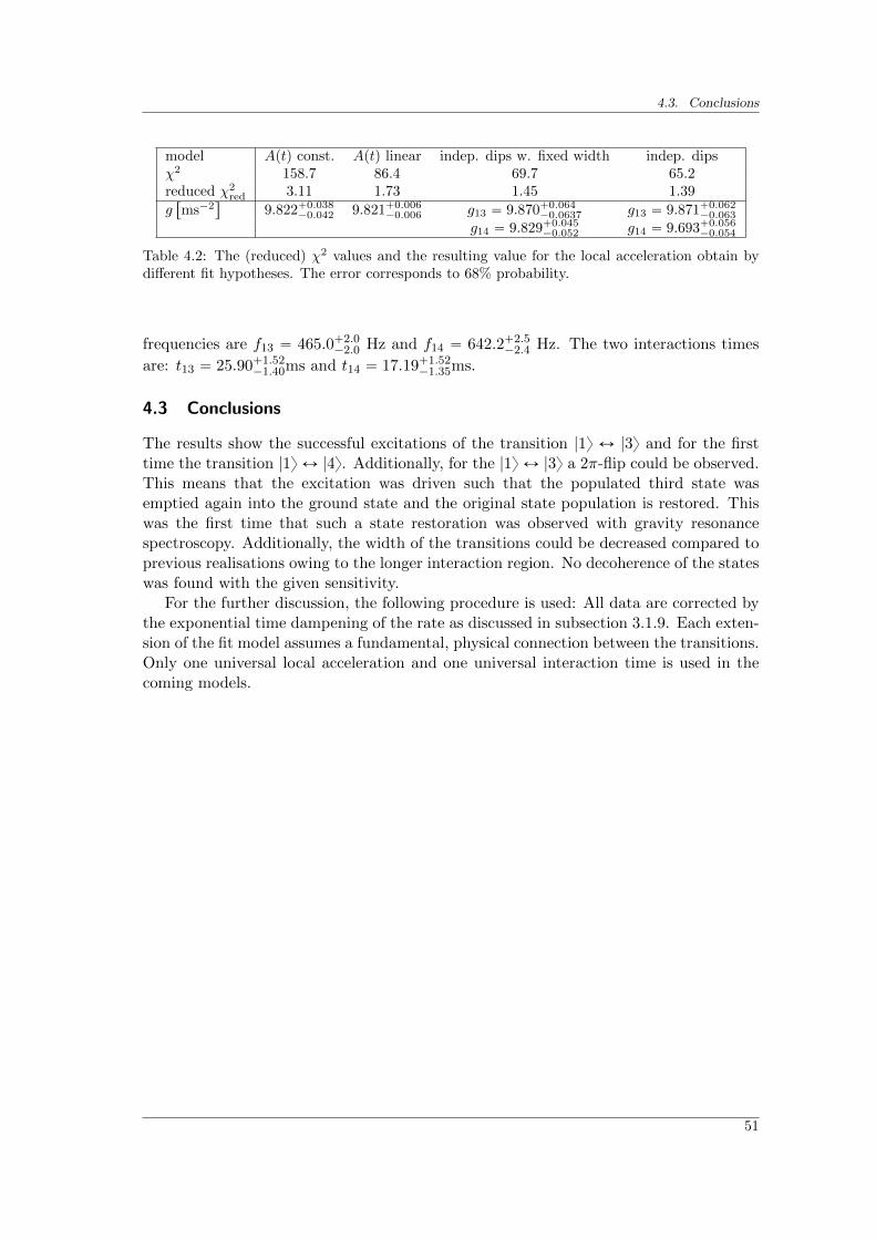
4.3. Conclusions
model Aptq const. Aptq linear indep. dips w. fixed width indep. dipsχ2 158.7 86.4 69.7 65.2reduced χ2
red 3.11 1.73 1.45 1.39
g“
ms´2‰
9.822`0.038´0.042 9.821`0.006
´0.006 g13 “ 9.870`0.064´0.0637 g13 “ 9.871`0.062
´0.063
g14 “ 9.829`0.045´0.052 g14 “ 9.693`0.056
´0.054
Table 4.2: The (reduced) χ2 values and the resulting value for the local acceleration obtain bydifferent fit hypotheses. The error corresponds to 68% probability.
frequencies are f13 “ 465.0`2.0´2.0 Hz and f14 “ 642.2`2.5
´2.4 Hz. The two interactions times
are: t13 “ 25.90`1.52´1.40ms and t14 “ 17.19`1.52
´1.35ms.
4.3 Conclusions
The results show the successful excitations of the transition |1y Ø |3y and for the firsttime the transition |1y Ø |4y. Additionally, for the |1y Ø |3y a 2π-flip could be observed.This means that the excitation was driven such that the populated third state wasemptied again into the ground state and the original state population is restored. Thiswas the first time that such a state restoration was observed with gravity resonancespectroscopy. Additionally, the width of the transitions could be decreased compared toprevious realisations owing to the longer interaction region. No decoherence of the stateswas found with the given sensitivity.
For the further discussion, the following procedure is used: All data are corrected bythe exponential time dampening of the rate as discussed in subsection 3.1.9. Each exten-sion of the fit model assumes a fundamental, physical connection between the transitions.Only one universal local acceleration and one universal interaction time is used in thecoming models.
51

Chapter 5
GRS Results
5.1 Determination of the local acceleration
By assuming known inertial and gravitational masses of the neutron, the experiment canserve as a gravimeter with a quantum object which determines the value for the localacceleration g. From the results presented in section 4.1, the experimentally derived localacceleration is g “ 9.844`0.035
´0.037ms2, for which this yields a successful test of Newton’sinverse square law at short distances.
5.2 Einstein equivalence principle
The history of the equivalence principle dates back to ancient Greece when Aristotlediscussed how objects fall. In his famous Physics he states that matter falls accordingto its mass. But already Philoponus, a philosopher who lived in Alexandria in the 6thcentury disagreed with Aristotle’s view [Rabinowitz, 2007]. The discussion became moresubstantial when Kepler found a description of the planet movements which did not needtheir masses. Well known is the test by Galileo by measuring the roll time of marbles onan inclined plane. Newton then provided the theory where the inertial mass mi, whichresists changes of movement and the gravitational mass mg, which interacts with thegravitational field, are equal.
In classical mechanics all particles in an external gravitational field are subject to thesame acceleration if their inertial and gravitational masses are equal which follows from:
mia “ mgg. (5.1)
In the following sections when talking about the gravitational mass, the passive grav-itational mass, which couples to an external field, is meant as opposed to the activemass, which generates a gravitational field. This implies that the back action of the testparticle mass on the field can be neglected, which is valid for the here discussed scenarioof a neutron in the gravity field: if we assume a neutron to be a homogeneous spherewith a radius rN “ 1 fm than the gravitational self energy is given by:
EG “ ´3
5Gm2N
rN“ ´7ˆ 10´31 J. (5.2)
53
Chapter 5. GRS Results
5.2.1 General relativity and the Einstein equivalence principle
In general relativity, formulated by Einstein, an observer is unable to distinguish betweenan accelerated and a free-falling reference frame. This cornerstone of general relativityleads to a geometrical interpretation of gravitation as a metric theory. If the back actionof test particle on the space-time geometry is sufficiently small, the equations of motionare independent of masses and each mass follows a geodetic.
The Einstein equivalence principle (EEP) leads to three different hypotheses [Giulini,2012]: The universality of free fall (UFF) or often called the weak equivalence principle(WEP), the local Lorentz invariance (LLI) and the local position invariance (LPI). Whilea geometric nature is sufficient to satisfy UFF, a metric theory is needed for EEP. Thethree hypotheses are of viable theoretical interest. Any violation of them would show thelimits in the validity of general relativity and hint to extensions of the theory. For ex-ample, time-varying fundamental constants would lead to composition dependent effectsand hence to violations of the UFF [Uzan, 2011].
Currently the UFF is the best tested part of this triple, see subsection 5.2.4. The LLIstates that local non-gravitational experiments have no preferred space-time direction. Itis tested to the level of 10´16 [Herrmann et al., 2005]. The LPI is commonly formulatedas universality of gravitational redshift (UGR) and universality of clock rates (UCR)which states that travelling different world lines between two events leads to the samered shift and two clocks agree upon travelling the same word line. They are tested to7ˆ 10´5 [Vessot et al., 1980] and p2˘ 4q ˆ 10´6 [Fortier et al., 2007] respectively.
5.2.2 Quantum mechanical tests of EEP
Gravitational effects on a quantum system were demonstrated with neutron interfero-metry, where two different flight paths in the gravity potential lead to a detectable phaseshift dependent on the mass of the neutron [Colella et al., 1975].
Another test is to let slow neutrons fall onto a liquid mirror from a variable height.As long as the kinetic energy gain from the fall is smaller than the Fermi potential ofthe liquid mirror, the neutron will be reflected of the surface and detected by a counter.While the free fall includes mg, the Fermi potential depends on mi (see section 2.1).This yields the inertial mass of the neutron to mi “ p1`p1.6˘ 2.5q ˆ 10´4qmg [Koester,1976] (but no rigorous test of the equivalence of the two masses). Additional work[Schmiedmayer, 1989] including scattering length determined with other experimentalsetups, derived the mass ratio
mgmi´ 1 “ p11˘ 17q ˆ 10´4. However some argue that this
test is not purely quantum as only the interaction with the reflecting material is witha quantum description, the free fall itself is in the classical limit [van der Zouw et al.,2000].
5.2.3 The quantum bouncer and universal free fall
[Greenberger, 1968] pointed out an intrinsic difference between GR and quantum mech-anics. So while in GR a particles trajectory is independent on the particle’s mass byconstruction using a geometrical structure, it enters in quantum mechanics due to quant-ization of various quantities. For example, the mass of an electron can be derived from
54
5.2. Einstein equivalence principle
its allowed orbits around a hydrogen nucleus. This means that quantities which areclassically kinematic can become depend on the mass.
Now we revisit the discussion of section 2.2 to introduce rigorously the inertial andgravitational masses. This follows the proposal of [Kajari et al., 2010]. The Schrodingerequation with the potential V pzq “ mg g z takes then the form:
ˆ
´~2
2mi
B2
Bz2`mggz
˙
ψnpzq “ Enψnpzq, (5.3)
where g “ GMC
RCoriginates only from the external gravity field. Solving the equation
above leads to the energy scale E0 and length scale z0, similar to equations 2.6:
E0 “3
d
~2m2gg
2
2mi, z0 “
3
d
~2
2mimgg. (5.4)
We are now in a situation to have two experimental parameters accessible where theinertial and gravitational mass enter in different relations. While gravity resonance spec-troscopy allows precise measurements of E0, experiments measuring the time evolutionof an UCN wave function after falling down a step provide accurate z0 values [Jenkeet al., 2009].
5.2.4 Limit on the Eotvosh parameter
Typically deviations on the WEP are normally parametrised by the Eotvosh parameterη. It describes the difference of acceleration a of two different test masses A and B,ideally at the same position to be subject to the same gravitational field, with differentchemical compositions.
η “ 2aA ´ aBaA ` aB
. (5.5)
The current limit of UFF, which is obtained by torsion pendulum experiments com-paring Beryllium and Titanium is η “ p0.8˘ 1.8q ˆ 10´13 [Schlamminger et al., 2008].As the test masses are macroscopic, this test is purely classical.
With gravity resonance spectroscopy, the Eotvosh parameter can derived from com-paring the local acceleration obtained from the transition frequencies and an externalclassical measurement. The local acceleration gspring was measured at the VCN exper-iment on the PF2 platform with a spring based WS 410/100 gravimeter. The valuegsp “ p9.805 07˘ 0.000 02qms´2 was obtained [Weber, 1998]. The uncertainty of thisvalue originates from the uncertainty of the absolute value measured at a reference pointin Grenoble that this relative measurement is referenced to. The uncertainty of the rel-ative measurements are several orders better. Comparing the two acceleration gives thefollowing Eotvosh parameter:
η “ p3.93˘ 3.80q ˆ 10´3. (5.6)
To put the result in perspective one should not forget that the gsp measurement is nearly20 years old and was conducted only in rough proximity to the actual GRS location.Over such a time frame it is not possible to reconstruct all potential changes in the
55
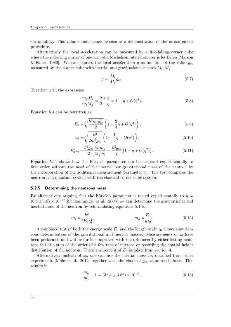
Chapter 5. GRS Results
surrounding. This value should hence be seen as a demonstration of the measurementprocedure.
Alternatively the local acceleration can be measured by a free-falling corner cubewhere the reflecting mirror of one arm of a Michelson interferometer is let fallen [Marson& Faller, 1986]. We can express the local acceleration g as function of the value gcc
measured by the corner cube with inertial and gravitational masses Mi,Mg:
g “Mi
Mggcc. (5.7)
Together with the expression
mgMi
miMg“
2` η
2´ η“ 1` η `Opη2q, (5.8)
Equation 5.4 can be rewritten as:
E0 “3
c
~2mig2cc
2
ˆ
1`2
3η `Opη2q
˙
, (5.9)
z0 “3
d
~2
2m2i gcc
ˆ
1´1
3η `Opη2q
˙
, (5.10)
E20z0 “
~2gcc
2
Mimg
Mgmi“
~2gcc
2
`
1` η `Opη2q˘
. (5.11)
Equation 5.11 shows how the Eotvosh parameter can be accessed experimentally tofirst order without the need of the inertial nor gravitational mass of the neutron bythe incorporation of the additional measurement parameter z0. The test compares theneutron as a quantum system with the classical corner-cube system.
5.2.5 Determining the neutrons mass
By alternatively arguing that the Eotvosh parameter is tested experimentally to η “p0.8˘ 1.8q ˆ 10´13 [Schlamminger et al., 2008] we can determine the gravitational andinertial mass of the neutron by reformulating equations 5.4 to:
mi “~2
2E0z20
, mg “E0
gz0. (5.12)
A combined test of both the energy scale E0 and the length scale z0 allows simultan-eous determination of the gravitational and inertial masses. Measurements of z0 havebeen performed and will be further improved with the qBouncer by either letting neut-rons fall of a step of the order of a few tens of microns or recording the spatial heightdistribution of the neutron. The measurement of E0 is taken from section 4.
Alternatively instead of z0, one can use the inertial mass mi obtained from otherexperiments [Mohr et al., 2012] together with the classical gsp value used above. Thisresults in
mg
mi´ 1 “ p3.94˘ 3.82q ˆ 10´3. (5.13)
56
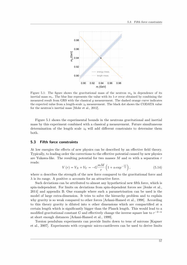
5.3. Fifth force constraints
energy meas.
length meas.
0.90 0.92 0.94 0.96 0.98
0.90
0.92
0.94
0.96
0.98
mi [GeV]
mg[GeV
]
Figure 5.1: The figure shows the gravitational mass of the neutron mg in dependence of itsinertial mass mi. The blue line represents the value with its 1-σ error obtained by combining themeasured result from GRS with the classical g measurement. The dashed orange curve indicatesthe expected value from a length-scale z0 measurement. The black dot shows the CODATA valuefor the neutron’s inertial mass [Mohr et al., 2012].
Figure 5.1 shows the experimental bounds in the neutrons gravitational and inertialmass by this experiment combined with a classical g measurement. Future simultaneousdetermination of the length scale z0 will add different constraints to determine themboth.
5.3 Fifth force constraints
At low energies the effects of new physics can be described by an effective field theory.Typically, to leading order the corrections to the effective potential caused by new physicsare Yukawa-like. The resulting potential for two masses M and m with a separation rreads:
V prq “ VN ` VY “ ´GmM
r
´
1` α exp´|r|λ
¯
, (5.14)
where α describes the strength of the new force compared to the gravitational force andλ is its range. A positive α accounts for an attractive force.
Such deviations can be attributed to almost any hypothetical new fifth force, which isspin-independent. For limits on deviations from spin-dependent forces see [Jenke et al.,2014] and appendix B. One example where such a parametrisation can be used is themodel of large extra-dimension. It tries to solve the hierarchy problem and to explainwhy gravity is so weak compared to other forces [Arkani-Hamed et al., 1998]. Accordingto this theory gravity is diluted into n other dimensions which are compactified at acertain length which is significantly bigger than the Planck length. This would lead to amodified gravitational constant G and effectively change the inverse square law to r´2´n
at short enough distances [Arkani-Hamed et al., 1999].Torsion pendulum experiments can provide limits down to tens of microns [Kapner
et al., 2007]. Experiments with cryogenic micro-cantilevers can be used to derive limits
57
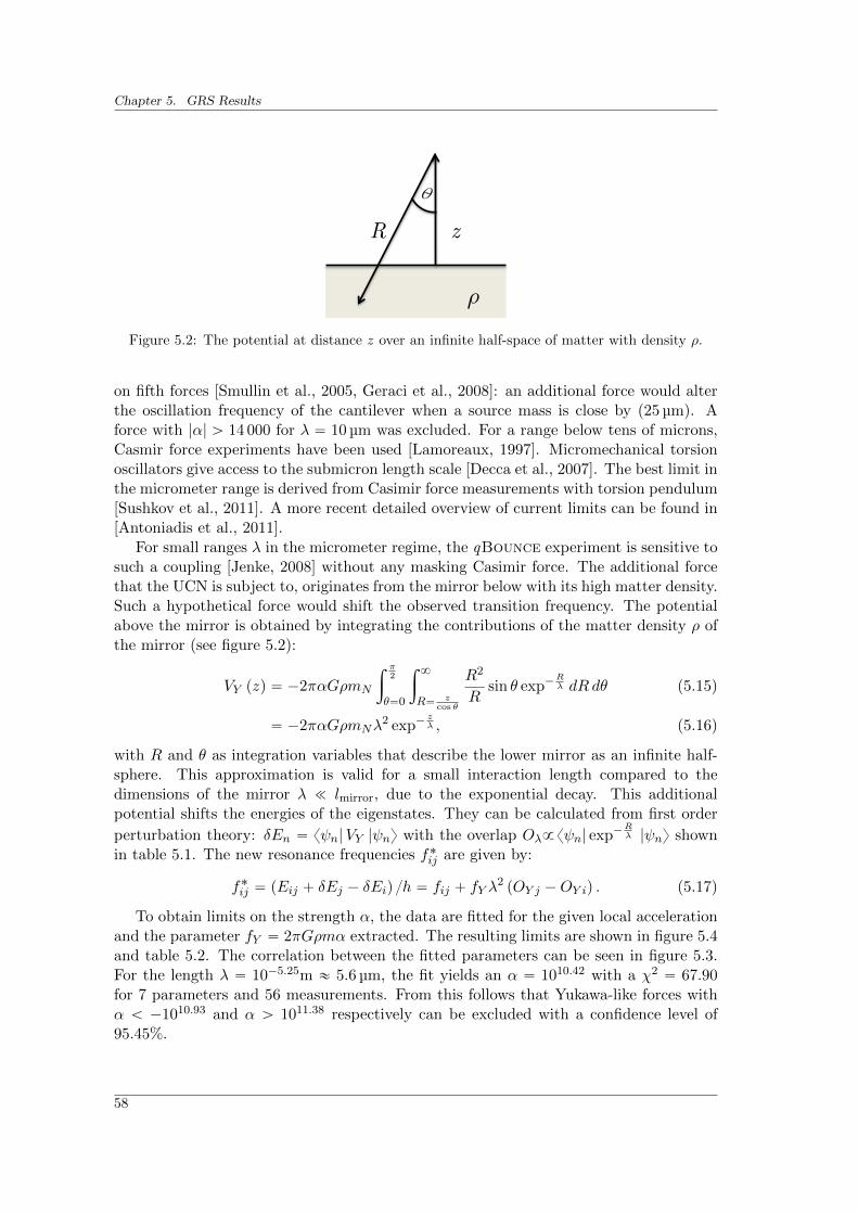
Chapter 5. GRS Results
ρ
R z
Ѳ
Figure 5.2: The potential at distance z over an infinite half-space of matter with density ρ.
on fifth forces [Smullin et al., 2005, Geraci et al., 2008]: an additional force would alterthe oscillation frequency of the cantilever when a source mass is close by (25 µm). Aforce with |α| ą 14 000 for λ “ 10 µm was excluded. For a range below tens of microns,Casmir force experiments have been used [Lamoreaux, 1997]. Micromechanical torsionoscillators give access to the submicron length scale [Decca et al., 2007]. The best limit inthe micrometer range is derived from Casimir force measurements with torsion pendulum[Sushkov et al., 2011]. A more recent detailed overview of current limits can be found in[Antoniadis et al., 2011].
For small ranges λ in the micrometer regime, the qBounce experiment is sensitive tosuch a coupling [Jenke, 2008] without any masking Casimir force. The additional forcethat the UCN is subject to, originates from the mirror below with its high matter density.Such a hypothetical force would shift the observed transition frequency. The potentialabove the mirror is obtained by integrating the contributions of the matter density ρ ofthe mirror (see figure 5.2):
VY pzq “ ´2παGρmN
ż π2
θ“0
ż 8
R“ zcos θ
R2
Rsin θ exp´
Rλ dRdθ (5.15)
“ ´2παGρmNλ2 exp´
zλ , (5.16)
with R and θ as integration variables that describe the lower mirror as an infinite half-sphere. This approximation is valid for a small interaction length compared to thedimensions of the mirror λ ! lmirror, due to the exponential decay. This additionalpotential shifts the energies of the eigenstates. They can be calculated from first order
perturbation theory: δEn “ xψn|VY |ψny with the overlap Oλ9xψn| exp´Rλ |ψny shown
in table 5.1. The new resonance frequencies f˚ij are given by:
f˚ij “ pEij ` δEj ´ δEiq h “ fij ` fY λ2 pOY j ´OY iq . (5.17)
To obtain limits on the strength α, the data are fitted for the given local accelerationand the parameter fY “ 2πGρmα extracted. The resulting limits are shown in figure 5.4and table 5.2. The correlation between the fitted parameters can be seen in figure 5.3.For the length λ “ 10´5.25m « 5.6 µm, the fit yields an α “ 1010.42 with a χ2 “ 67.90for 7 parameters and 56 measurements. From this follows that Yukawa-like forces withα ă ´1010.93 and α ą 1011.38 respectively can be excluded with a confidence level of95.45%.
58
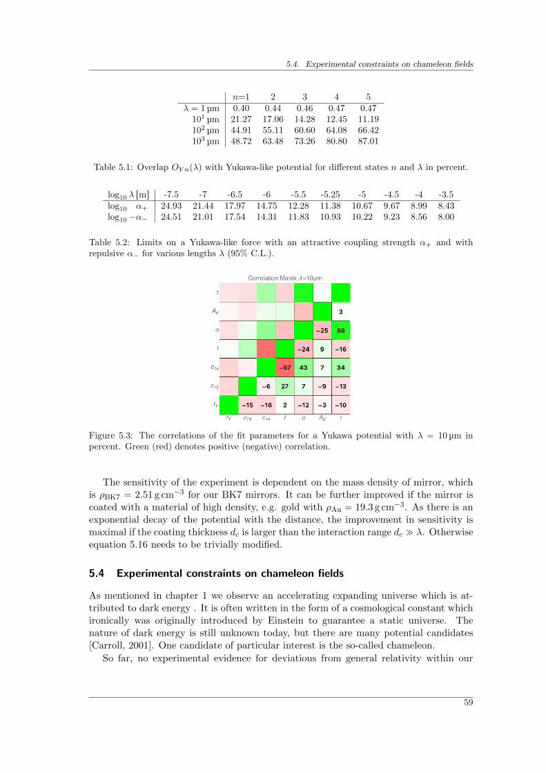
5.4. Experimental constraints on chameleon fields
n=1 2 3 4 5λ “ 1 µm 0.40 0.44 0.46 0.47 0.47
101 µm 21.27 17.06 14.28 12.45 11.19102 µm 44.91 55.11 60.60 64.08 66.42103 µm 48.72 63.48 73.26 80.80 87.01
Table 5.1: Overlap OY npλq with Yukawa-like potential for different states n and λ in percent.
log10 λ rms -7.5 -7 -6.5 -6 -5.5 -5.25 -5 -4.5 -4 -3.5log10 α` 24.93 21.44 17.97 14.75 12.28 11.38 10.67 9.67 8.99 8.43log10´α´ 24.51 21.01 17.54 14.31 11.83 10.93 10.22 9.23 8.56 8.00
Table 5.2: Limits on a Yukawa-like force with an attractive coupling strength α` and withrepulsive α´ for various lengths λ (95% C.L.).
Figure 5.3: The correlations of the fit parameters for a Yukawa potential with λ “ 10 µm inpercent. Green (red) denotes positive (negative) correlation.
The sensitivity of the experiment is dependent on the mass density of mirror, whichis ρBK7 “ 2.51 g cm´3 for our BK7 mirrors. It can be further improved if the mirror iscoated with a material of high density, e.g. gold with ρAu “ 19.3 g cm´3. As there is anexponential decay of the potential with the distance, the improvement in sensitivity ismaximal if the coating thickness dc is larger than the interaction range dc " λ. Otherwiseequation 5.16 needs to be trivially modified.
5.4 Experimental constraints on chameleon fields
As mentioned in chapter 1 we observe an accelerating expanding universe which is at-tributed to dark energy . It is often written in the form of a cosmological constant whichironically was originally introduced by Einstein to guarantee a static universe. Thenature of dark energy is still unknown today, but there are many potential candidates[Carroll, 2001]. One candidate of particular interest is the so-called chameleon.
So far, no experimental evidence for deviations from general relativity within our
59
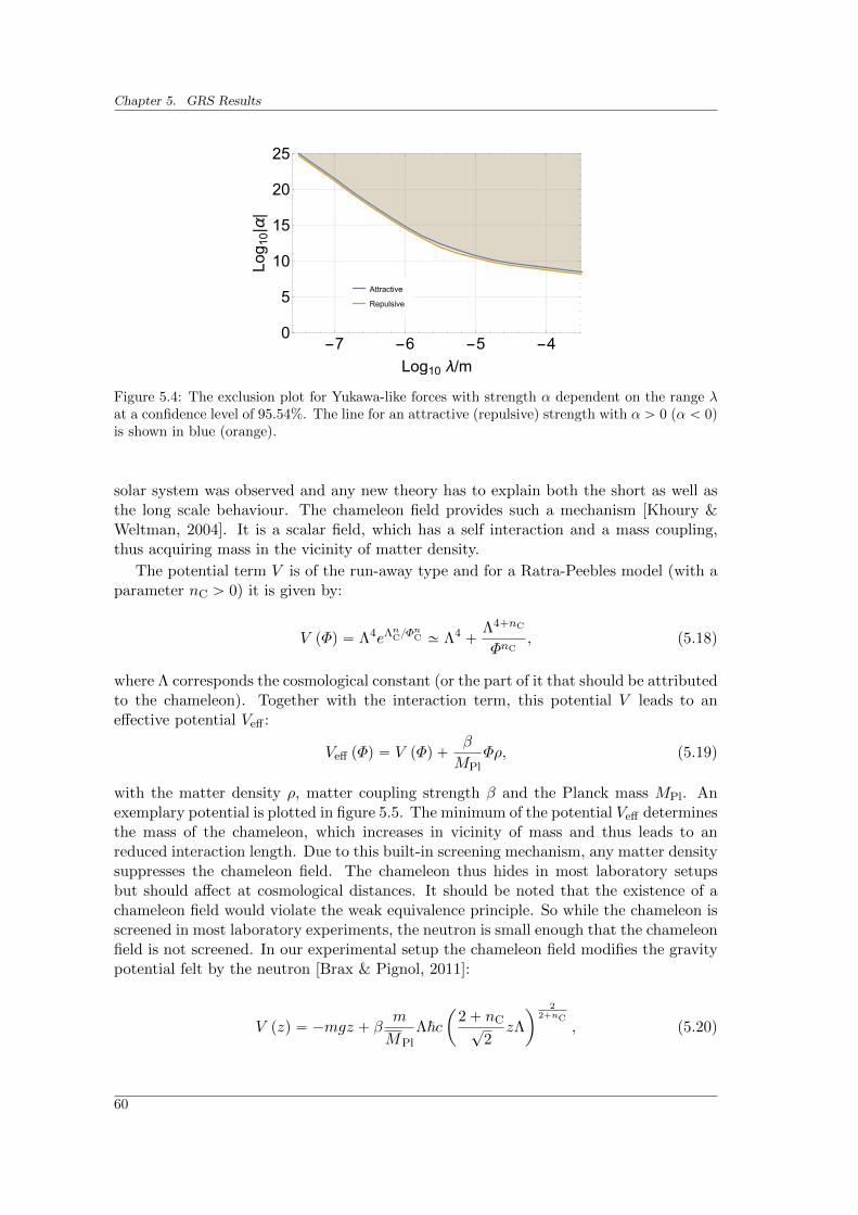
Chapter 5. GRS Results
Attractive
Repulsive
-7 -6 -5 -40
5
10
15
20
25
Log10 λ/m
Log 10|α|
Figure 5.4: The exclusion plot for Yukawa-like forces with strength α dependent on the range λat a confidence level of 95.54%. The line for an attractive (repulsive) strength with α ą 0 (α ă 0)is shown in blue (orange).
solar system was observed and any new theory has to explain both the short as well asthe long scale behaviour. The chameleon field provides such a mechanism [Khoury &Weltman, 2004]. It is a scalar field, which has a self interaction and a mass coupling,thus acquiring mass in the vicinity of matter density.
The potential term V is of the run-away type and for a Ratra-Peebles model (with aparameter nC ą 0) it is given by:
V pΦq “ Λ4eΛnCΦnC » Λ4 `
Λ4`nC
ΦnC, (5.18)
where Λ corresponds the cosmological constant (or the part of it that should be attributedto the chameleon). Together with the interaction term, this potential V leads to aneffective potential Veff :
Veff pΦq “ V pΦq `β
MPlΦρ, (5.19)
with the matter density ρ, matter coupling strength β and the Planck mass MPl. Anexemplary potential is plotted in figure 5.5. The minimum of the potential Veff determinesthe mass of the chameleon, which increases in vicinity of mass and thus leads to anreduced interaction length. Due to this built-in screening mechanism, any matter densitysuppresses the chameleon field. The chameleon thus hides in most laboratory setupsbut should affect at cosmological distances. It should be noted that the existence of achameleon field would violate the weak equivalence principle. So while the chameleon isscreened in most laboratory experiments, the neutron is small enough that the chameleonfield is not screened. In our experimental setup the chameleon field modifies the gravitypotential felt by the neutron [Brax & Pignol, 2011]:
V pzq “ ´mgz ` βm
MPl
Λ~cˆ
2` nC?
2zΛ
˙2
2`nC
, (5.20)
60
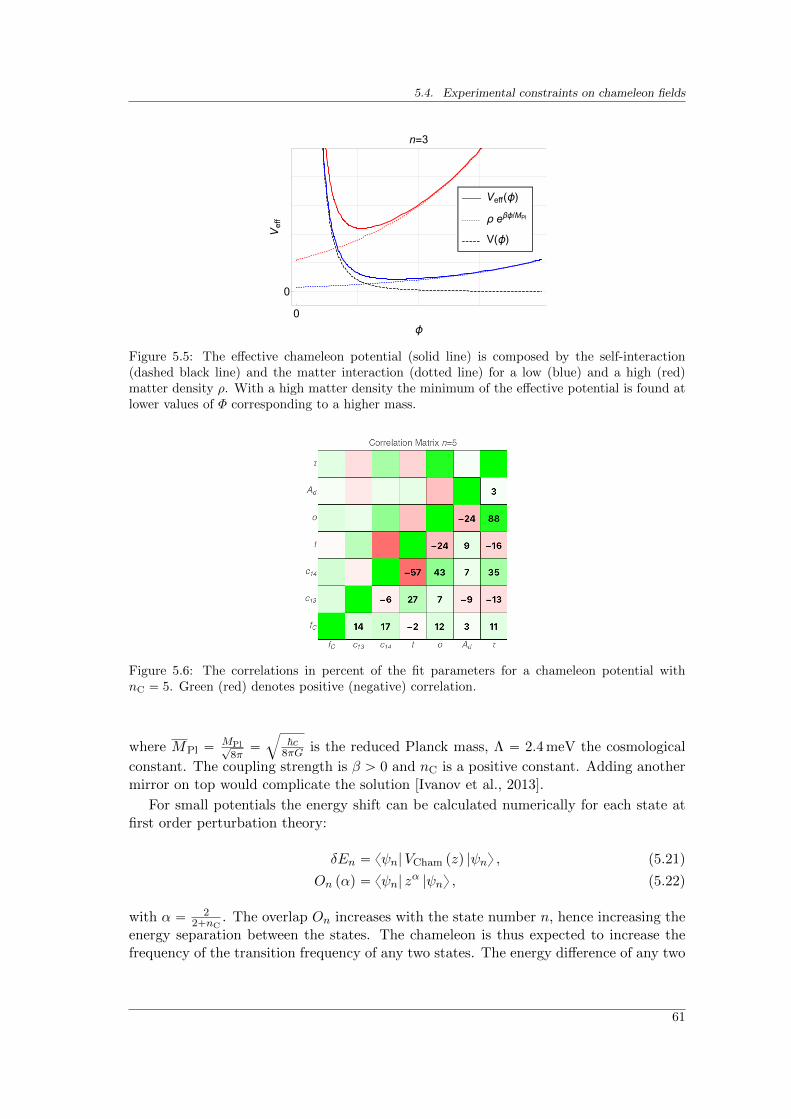
5.4. Experimental constraints on chameleon fields
Veff(ϕ)
ρ eβϕ/MPl
V(ϕ)
0
0
ϕ
Veff
n=3
Figure 5.5: The effective chameleon potential (solid line) is composed by the self-interaction(dashed black line) and the matter interaction (dotted line) for a low (blue) and a high (red)matter density ρ. With a high matter density the minimum of the effective potential is found atlower values of Φ corresponding to a higher mass.
Figure 5.6: The correlations in percent of the fit parameters for a chameleon potential withnC “ 5. Green (red) denotes positive (negative) correlation.
where MPl “MPl?
8π“
b
~c8πG is the reduced Planck mass, Λ “ 2.4 meV the cosmological
constant. The coupling strength is β ą 0 and nC is a positive constant. Adding anothermirror on top would complicate the solution [Ivanov et al., 2013].
For small potentials the energy shift can be calculated numerically for each state atfirst order perturbation theory:
δEn “ xψn|VCham pzq |ψny , (5.21)
On pαq “ xψn| zα |ψny , (5.22)
with α “ 22`nC
. The overlap On increases with the state number n, hence increasing theenergy separation between the states. The chameleon is thus expected to increase thefrequency of the transition frequency of any two states. The energy difference of any two
61
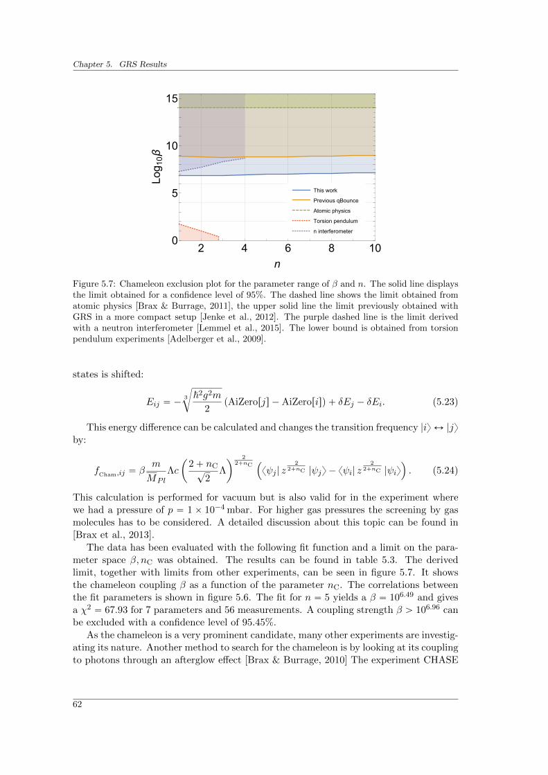
Chapter 5. GRS Results
This work
Previous qBounce
Atomic physics
Torsion pendulum
n interferometer
2 4 6 8 100
5
10
15
n
Log 10β
Figure 5.7: Chameleon exclusion plot for the parameter range of β and n. The solid line displaysthe limit obtained for a confidence level of 95%. The dashed line shows the limit obtained fromatomic physics [Brax & Burrage, 2011], the upper solid line the limit previously obtained withGRS in a more compact setup [Jenke et al., 2012]. The purple dashed line is the limit derivedwith a neutron interferometer [Lemmel et al., 2015]. The lower bound is obtained from torsionpendulum experiments [Adelberger et al., 2009].
states is shifted:
Eij “ ´3
c
~2g2m
2pAiZerorjs ´AiZerorisq ` δEj ´ δEi. (5.23)
This energy difference can be calculated and changes the transition frequency |iy Ø |jyby:
fCham,ij “ β
m
MPl
Λc
ˆ
2` nC?
2Λ
˙2
2`nC´
xψj | z2
2`nC |ψjy ´ xψi| z2
2`nC |ψiy¯
. (5.24)
This calculation is performed for vacuum but is also valid for in the experiment wherewe had a pressure of p “ 1ˆ 10´4 mbar. For higher gas pressures the screening by gasmolecules has to be considered. A detailed discussion about this topic can be found in[Brax et al., 2013].
The data has been evaluated with the following fit function and a limit on the para-meter space β, nC was obtained. The results can be found in table 5.3. The derivedlimit, together with limits from other experiments, can be seen in figure 5.7. It showsthe chameleon coupling β as a function of the parameter nC. The correlations betweenthe fit parameters is shown in figure 5.6. The fit for n “ 5 yields a β “ 106.49 and givesa χ2 “ 67.93 for 7 parameters and 56 measurements. A coupling strength β ą 106.96 canbe excluded with a confidence level of 95.45%.
As the chameleon is a very prominent candidate, many other experiments are investig-ating its nature. Another method to search for the chameleon is by looking at its couplingto photons through an afterglow effect [Brax & Burrage, 2010] The experiment CHASE
62
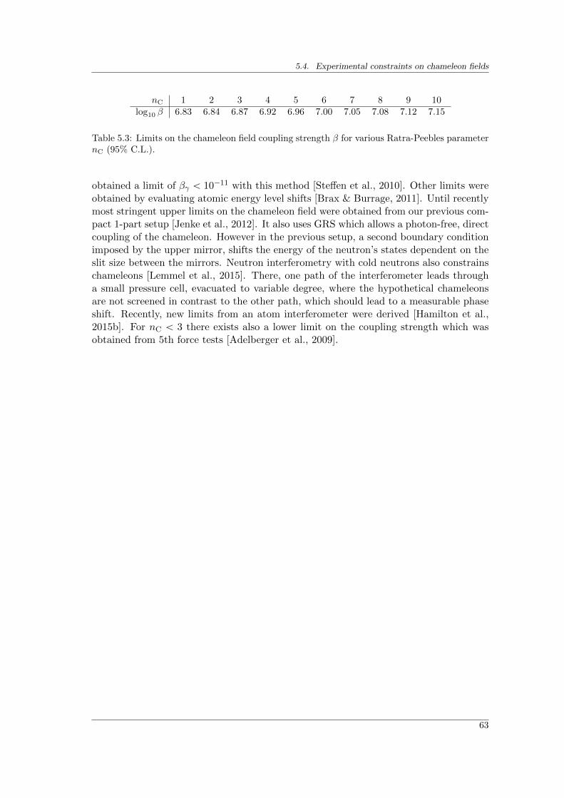
5.4. Experimental constraints on chameleon fields
nC 1 2 3 4 5 6 7 8 9 10log10 β 6.83 6.84 6.87 6.92 6.96 7.00 7.05 7.08 7.12 7.15
Table 5.3: Limits on the chameleon field coupling strength β for various Ratra-Peebles parameternC (95% C.L.).
obtained a limit of βγ ă 10´11 with this method [Steffen et al., 2010]. Other limits wereobtained by evaluating atomic energy level shifts [Brax & Burrage, 2011]. Until recentlymost stringent upper limits on the chameleon field were obtained from our previous com-pact 1-part setup [Jenke et al., 2012]. It also uses GRS which allows a photon-free, directcoupling of the chameleon. However in the previous setup, a second boundary conditionimposed by the upper mirror, shifts the energy of the neutron’s states dependent on theslit size between the mirrors. Neutron interferometry with cold neutrons also constrainschameleons [Lemmel et al., 2015]. There, one path of the interferometer leads througha small pressure cell, evacuated to variable degree, where the hypothetical chameleonsare not screened in contrast to the other path, which should lead to a measurable phaseshift. Recently, new limits from an atom interferometer were derived [Hamilton et al.,2015b]. For nC ă 3 there exists also a lower limit on the coupling strength which wasobtained from 5th force tests [Adelberger et al., 2009].
63

Chapter 6
Summary & Outlook
With the setup presented here, the technique of Gravity Resonance Spectroscopy wasfurther improved. The previously limiting systematic factor, an upper mirror in theinteraction region could be spared by realising a three-part setup. While being sys-tematically more appealing, it increased the experimental complexity of the experiment.New techniques were incorporated and the setup was modified at many different areas.Additionally the influences of the changed layout were evaluated, like the eigen basischanges between regions, alignment influences and confinement of the oscillation.
With the new setup and the increased interaction time transitions between the states|1y Ø |3y and |1y Ø |4y could be studied, the latter for the first time in GRS. Anotherfirst is the observed state revival of the ground state upon a π-flip for the transition|1y Ø |3y. Driving the oscillation sufficiently strong the original state population ofthe first and the excited third state could be restored. The observed energy resolutionof these transitions was ∆E13 “ 5ˆ 10´15 eV and ∆E14 “ 7ˆ 10´15 eV (1-σ standarddeviation). This is a feature that is only possible with the new three part setup whichdoes not add any dampening in the interaction region (and further improved setups tocome in the future). No decoherence of the states was observed with this setup.
With this experiment, the natural length scale E0 of a gravitationally bound ultra-coldneutron is easily accessible. This allows to study the connection of the local accelera-tion, the neutrons gravitational and inertial mass and Planck’s constant. The measuredlocal acceleration can be compared with the value obtained in a classical measurementto test the weak equivalence principle or to derive the gravitational mass of the neutron.New experiments within the qBounce collaboration will further enrich this discussionby determining the natural length scale z0 with increased precision. Hypothetical devi-ations of Newton’s inverse square law of gravity at the micrometer length scale are ofavid interest for the community searching for extensions of the standard model. Suchnew forces are in the sensitivity range of the experiment and limits for a special para-metrisation with the form of a Yukawa-like potential have been derived. Furthermore,the observed transitions were used to derive limits on the scalar chameleon field, a verypopular candidate for dark energy. While not the most stringent ones, they are morerigorous than previous limits obtained from neutron physics.
Following the lessons learned from expanding the setup, the next technological leap
65
Chapter 6. Summary & Outlook
lays ahead as the implementation of Gravity Resonance Spectroscopy with a Ramsey-like setup [Ramsey, 1956]. The advantages this step will bring, like self-focussing velocityinsensitivity and even longer propagation times, face the challenging task of maintainingthe borderline low neutron flux [Abele et al., 2010]. New ultra-cold neutron sources witha higher flux might help to facilitate the external time constrains of this class of experi-ments. Furthermore, a Ramsey-like setup would also allow, with some modifications, totest the neutrons charge [Durstberger-Rennhofer et al., 2011].
66

Appendices
67

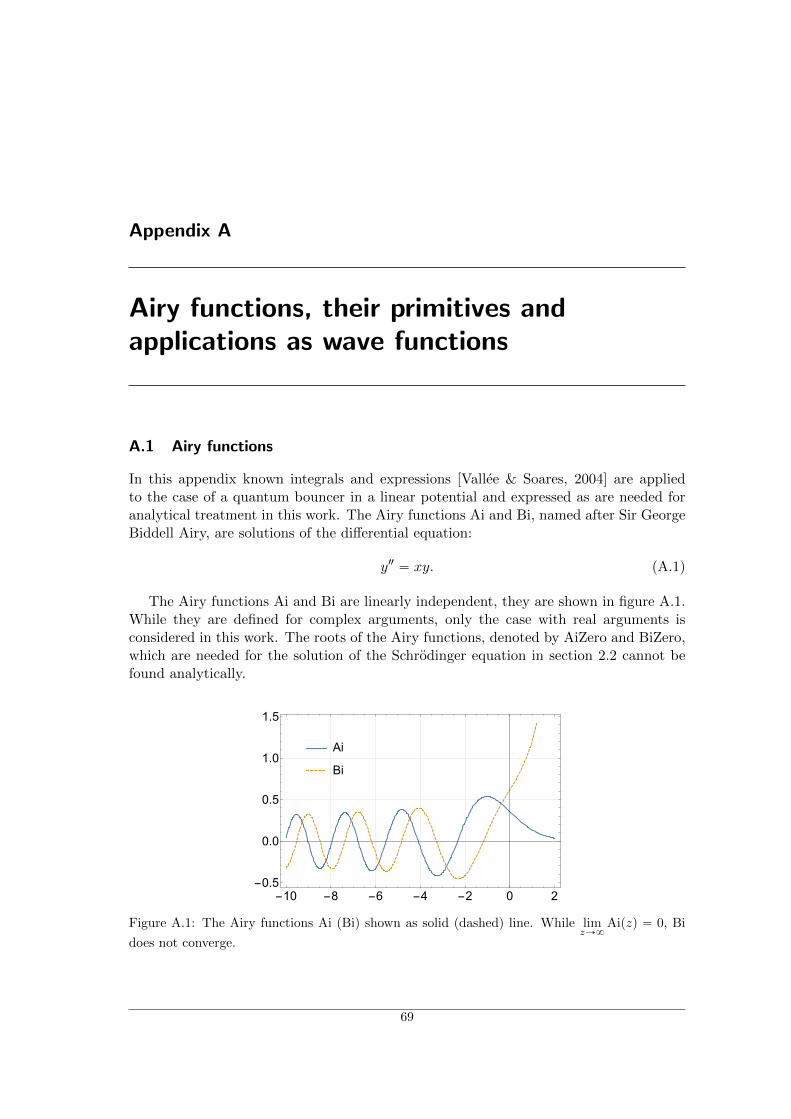
Appendix A
Airy functions, their primitives andapplications as wave functions
A.1 Airy functions
In this appendix known integrals and expressions [Vallee & Soares, 2004] are appliedto the case of a quantum bouncer in a linear potential and expressed as are needed foranalytical treatment in this work. The Airy functions Ai and Bi, named after Sir GeorgeBiddell Airy, are solutions of the differential equation:
y2 “ xy. (A.1)
The Airy functions Ai and Bi are linearly independent, they are shown in figure A.1.While they are defined for complex arguments, only the case with real arguments isconsidered in this work. The roots of the Airy functions, denoted by AiZero and BiZero,which are needed for the solution of the Schrodinger equation in section 2.2 cannot befound analytically.
Ai
Bi
-10 -8 -6 -4 -2 0 2-0.5
0.0
0.5
1.0
1.5
Figure A.1: The Airy functions Ai (Bi) shown as solid (dashed) line. While limzÑ8
Aipzq “ 0, Bi
does not converge.
69
Appendix A. Airy functions, their primitives and applications as wave functions
A.2 Overlap of Airy functions
The overlap of different linear combinations A, B of Airy functions Ai and Bi can becalculated by:
ż
A pα pz ` βqqB pα pz ` βqq dz “
pz ` βqA pα pz ` βqqB pα pz ` βqq ´1
αA1 pα pz ` βqqB1 pα pz ` βqq (A.2)
A more general form for different arguments reads:
ż
A pα pz ` β1qqB pα pz ` β2qq dz “
1
α2 pβ1 ´ β2qtA1 pα pz ` β1qqB pα pz ` β2qq ´A pα pz ` β1qqB1 pα pz ` β2qqu (A.3)
A.3 The free wave function
The wave function of a neutron in the gravity field, which fulfils the Schrodinger equationreads:
ψn pzq “ cnAi
ˆ
z
z0`AiZero pnq
˙
, (A.4)
where z is the vertical coordinate, z0 is the length scale that scales the Airy functionaccordingly to the physical system (see equation 2.5). The wave function of the n-thstate is a Airy function shifted by the n-th root. This ensures that the wave functionfulfils the boundary condition ψpz “ 0q “ 0. The eigen energy of the state is given by
En “ ´AiZero pnq ¨ E0, (A.5)
with the energy scale E0 of the system.To obtain the normalisation constant cn in equation A.4, the definite integral given
in equation A.2 can be used with the limits limzÑ8
zAi2 pzq “ 0 and limzÑ8
Ai12 pzq “ 0:
ż 8
0Ai2
ˆ
z
z0`AiZero pnq
˙
dz “ z0Ai12pAiZero pnqq . (A.6)
Demanding that the wave function squared has to be unity |ψn pzq |2 “ 1 gives the
normalisation constant cn with dimension L´12:
cn “ 1
b
z0Ai12 pAiZero pnqq. (A.7)
A.4 The wave function with upper mirror
When a second mirror at height l confines the neutron from above, an additional bound-ary condition has to be satisfied φpz “ lq “ 0. The wave function of a neutron in thegravity field with an additional boundary condition then reads:
φn pzq “ anAi
ˆ
z
z0´E1nE0
˙
` bnBi
ˆ
z
z0´E1nE0
˙
. (A.8)
70
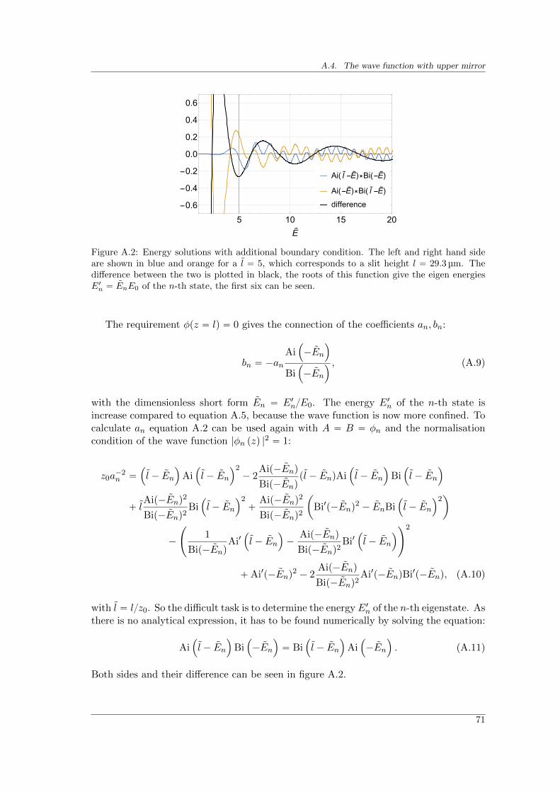
A.4. The wave function with upper mirror
Ai( l˜-E˜)⨯Bi(-E
˜)
Ai(-E˜)⨯Bi( l
˜-E˜)
difference
5 10 15 20
-0.6
-0.4
-0.2
0.0
0.2
0.4
0.6
E˜
Figure A.2: Energy solutions with additional boundary condition. The left and right hand sideare shown in blue and orange for a l “ 5, which corresponds to a slit height l “ 29.3 µm. Thedifference between the two is plotted in black, the roots of this function give the eigen energiesE1n “ EnE0 of the n-th state, the first six can be seen.
The requirement φpz “ lq “ 0 gives the connection of the coefficients an, bn:
bn “ ´anAi
´
´En
¯
Bi´
´En
¯ , (A.9)
with the dimensionless short form En “ E1nE0. The energy E1n of the n-th state isincrease compared to equation A.5, because the wave function is now more confined. Tocalculate an equation A.2 can be used again with A “ B “ φn and the normalisationcondition of the wave function |φn pzq |
2 “ 1:
z0a´2n “
´
l ´ En
¯
Ai´
l ´ En
¯2´ 2
Aip´Enq
Bip´Enqpl ´ EnqAi
´
l ´ En
¯
Bi´
l ´ En
¯
` lAip´Enq
2
Bip´Enq2Bi
´
l ´ En
¯2`
Aip´Enq2
Bip´Enq2
ˆ
Bi1p´Enq2 ´ EnBi
´
l ´ En
¯2˙
´
˜
1
Bip´EnqAi1
´
l ´ En
¯
´Aip´Enq
Bip´Enq2Bi1
´
l ´ En
¯
¸2
`Ai1p´Enq2 ´ 2
Aip´Enq
Bip´Enq2Ai1p´EnqBi1p´Enq, (A.10)
with l “ lz0. So the difficult task is to determine the energy E1n of the n-th eigenstate. Asthere is no analytical expression, it has to be found numerically by solving the equation:
Ai´
l ´ En
¯
Bi´
´En
¯
“ Bi´
l ´ En
¯
Ai´
´En
¯
. (A.11)
Both sides and their difference can be seen in figure A.2.
71
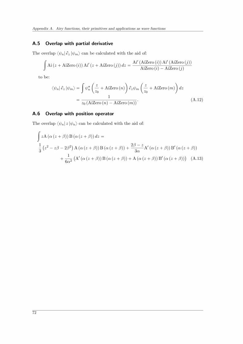
Appendix A. Airy functions, their primitives and applications as wave functions
A.5 Overlap with partial derivative
The overlap xψn| Bz |ψmy can be calculated with the aid of:
ż
Ai pz `AiZero piqqAi1 pz `AiZero pjqq dz “Ai1 pAiZero piqqAi1 pAiZero pjqq
AiZero piq ´AiZero pjq
to be:
xψn| Bz |ψmy “
ż
ψ˚n
ˆ
z
z0`AiZero pnq
˙
Bzψm
ˆ
z
z0`AiZero pmq
˙
dz
“1
z0 pAiZero pnq ´AiZero pmqq. (A.12)
A.6 Overlap with position operator
The overlap xψn| z |ψny can be calculated with the aid of:
ż
zA pα pz ` βqqB pα pz ` βqq dz “
1
3
`
z2 ´ zβ ´ 2β2˘
A pα pz ` βqqB pα pz ` βqq `2β ´ z
3αA1 pα pz ` βqqB1 pα pz ` βqq
`1
6α2
`
A1 pα pz ` βqqB pα pz ` βqq `A pα pz ` βqqB1 pα pz ` βqq˘
(A.13)
72
Appendix B
Characterisation of polarisation foil
B.1 Motivation
To search for deviations from gravity which are caused by spin-dependent forces one canmake use of the neutron spin. Any spin-coupling field would modify the eigen energiesof the gravitational states dependent on their spin orientation. Searches for such a spin-coupling field have been carried out at the Institut Laue-Langevin (ILL) with gravityresonance spectroscopy and derived limits on axion-like particles [Jenke et al., 2014].
Experimental modifications of the setup were required to search for an additional spin-coupling. A magnetic guiding field was installed and the entrance foil of the detector wascoated to ensure only one polarisation was able to enter the detector and be recorded.The resonance curve was measured for both spin polarisations by reversing the magneticfield and the polariser. Missing deviations between these measurements lead to limits onspin-coupling fields.
B.2 Characterisation of a polariser
B.2.1 Functioning of the polariser
The polariser is realised by a modification of the detector entrance foil. The entrancefoil, separating the vacuum from the detector volume filled with ArCO2 is coated onthe inside with 10B to convert ultra-cold neutrons into charged particles, see chapter3.1.5. To allow only one spin orientation to enter the detector, the outside of the foil wascoated with soft iron. The coating was done by Th. Lauers group1. When the soft ironis polarised, the potential V˘ of the material V˘ as seen by each orientation is given bythe Fermi potential VF modified by an additional spin-dependent part (see 2.1):
V˘ “ VF ˘ µB, (B.1)
where µ is the UCNs magnetic moment and B the internal magnetic field of the coating.If the neutron spin is anti-/parallel to the foil polarisation, the Fermi potential is in-/decreased. In each case, UCNs can pass the foil only if their velocity exceeds the
1At the time of testing associated at the Institut fur Physik, Universitat Mainz, Germany.
73
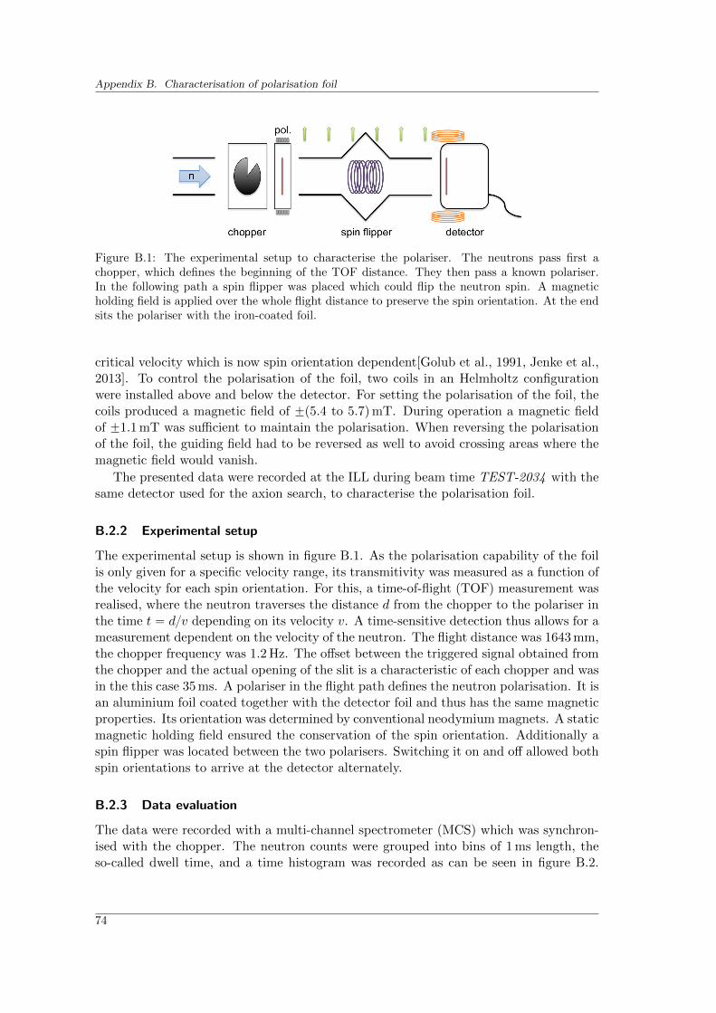
Appendix B. Characterisation of polarisation foil
Figure B.1: The experimental setup to characterise the polariser. The neutrons pass first achopper, which defines the beginning of the TOF distance. They then pass a known polariser.In the following path a spin flipper was placed which could flip the neutron spin. A magneticholding field is applied over the whole flight distance to preserve the spin orientation. At the endsits the polariser with the iron-coated foil.
critical velocity which is now spin orientation dependent[Golub et al., 1991, Jenke et al.,2013]. To control the polarisation of the foil, two coils in an Helmholtz configurationwere installed above and below the detector. For setting the polarisation of the foil, thecoils produced a magnetic field of ˘p5.4 to 5.7qmT. During operation a magnetic fieldof ˘1.1 mT was sufficient to maintain the polarisation. When reversing the polarisationof the foil, the guiding field had to be reversed as well to avoid crossing areas where themagnetic field would vanish.
The presented data were recorded at the ILL during beam time TEST-2034 with thesame detector used for the axion search, to characterise the polarisation foil.
B.2.2 Experimental setup
The experimental setup is shown in figure B.1. As the polarisation capability of the foilis only given for a specific velocity range, its transmitivity was measured as a function ofthe velocity for each spin orientation. For this, a time-of-flight (TOF) measurement wasrealised, where the neutron traverses the distance d from the chopper to the polariser inthe time t “ dv depending on its velocity v. A time-sensitive detection thus allows for ameasurement dependent on the velocity of the neutron. The flight distance was 1643 mm,the chopper frequency was 1.2 Hz. The offset between the triggered signal obtained fromthe chopper and the actual opening of the slit is a characteristic of each chopper and wasin the this case 35 ms. A polariser in the flight path defines the neutron polarisation. It isan aluminium foil coated together with the detector foil and thus has the same magneticproperties. Its orientation was determined by conventional neodymium magnets. A staticmagnetic holding field ensured the conservation of the spin orientation. Additionally aspin flipper was located between the two polarisers. Switching it on and off allowed bothspin orientations to arrive at the detector alternately.
B.2.3 Data evaluation
The data were recorded with a multi-channel spectrometer (MCS) which was synchron-ised with the chopper. The neutron counts were grouped into bins of 1 ms length, theso-called dwell time, and a time histogram was recorded as can be seen in figure B.2.
74
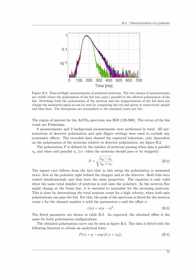
B.2. Characterisation of a polariser
Figure B.2: Time-of-flight measurements of polarised neutrons. The two classes of measurementsare visible where the polarisation of the foil was (anti-) parallel to the allowed polarisation of thefoil. Switching both the polarisation of the neutron and the magnetisation of the foil does notchange the measured signal as can be seen by comparing the red and green or respectively purpleand blue lines. The histograms are normalised to the maximal count per bin.
The region of interest for the ArCO2 spectrum was ROI (128-900). The errors of the bincount are Poissonian.
8 measurements and 2 background measurements were performed in total. All per-mutations of detector polarisation and spin flipper settings were used to exclude anysystematic effects. The recorded data showed the expected behaviour, only dependenton the polarisation of the neutrons relative to detector polarisation, see figure B.2.
The polarisation P is defined by the number of neutrons passing when spin is parallelnp and when anti parallel ns (i.e. when the neutrons should pass or be stopped):
P “
d
np ´ nsnp ` ns
. (B.2)
The square root follows from the fact that in this setup the polarisation is measuredtwice: first at the polariser right behind the chopper and at the detector. Both foils werecoated simultaneously and thus have the same properties. The equation is only validwhen the same total number of neutrons is sent onto the polariser. As the neutron fluxmight change at the beam line, it is essential to normalise for the incoming neutrons.This is done by determining the total neutron count for a high velocity, when both spinpolarisations can pass the foil. For this, the peak of the spectrum is fitted for the neutroncount c for the channel number n with the parameters a and the offset o:
cpnq “ apn´ oq2. (B.3)
The fitted parameter are shown in table B.3. As expected, the obtained offset is thesame for both polarisation configurations.
The obtained polarisation curve can be seen in figure B.4. The data is fitted with thefollowing function to obtain an analytical form:
P pvq “ p´ exp pk pv ` v0qq . (B.4)
75
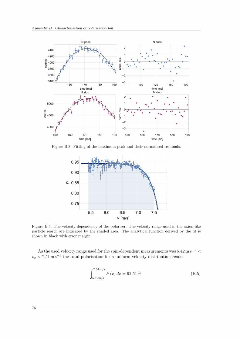
Appendix B. Characterisation of polarisation foil
160 170 180 1903400
3600
3800
4000
4200
4400
time [ms]
counts
N pass
160 170 180 190-3
-2
-1
0
1
2
time [ms]
norm.res.
N pass
150 160 170 180 190
4000
4500
5000
time [ms]
counts
N stop
150 160 170 180 190
-3
-2
-1
0
1
2
time [ms]
norm.res.
N stop
Figure B.3: Fitting of the maximum peak and their normalised residuals.
5.5 6.0 6.5 7.0 7.5
0.75
0.80
0.85
0.90
0.95
v [m/s]
P
Figure B.4: The velocity dependency of the polariser. The velocity range used in the axion-likeparticle search are indicated by the shaded area. The analytical function derived by the fit isshown in black with error margin.
As the used velocity range used for the spin-dependent measurements was 5.42 m s´1 ă
vx ă 7.51 m s´1 the total polarisation for a uniform velocity distribution reads:
ż 7.51ms
5.42msP pvq dv “ 92.51 %. (B.5)
76
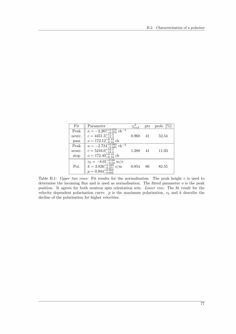
B.2. Characterisation of a polariser
Fit Parameter χ2red pts prob. r%s
Peak a “ ´2.267`0.078´0.078 ch´2
neutr. c “ 4451.3`15.3´15.3 0.968 41 52.54
pass o “ 172.12`0.19´0.18 ch
Peak a “ ´2.724`0.085´0.085 ch´2
neutr. c “ 5216.0`16.4´16.4 1.288 41 11.03
stop o “ 172.40`0.18´0.18 ch
v0 “ ´8.01`0.04´0.04 m/s
Pol. k “ 3.826`0.289´0.271 s/m 0.854 86 82.55
p “ 0.944`0.002´0.002
Table B.1: Upper two rows: Fit results for the normalisation. The peak height c is used todetermine the incoming flux and is used as normalisation. The fitted parameter o is the peakposition. It agrees for both neutron spin orientation sets. Lower row: The fit result for thevelocity dependent polarisation curve. p is the maximum polarisation, v0 and k describe thedecline of the polarisation for higher velocities.
77

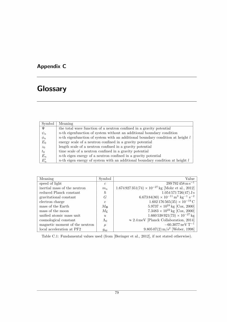
Appendix C
Glossary
Symbol MeaningΨ the total wave function of a neutron confined in a gravity potentialψn n-th eigenfunction of system without an additional boundary conditionφn n-th eigenfunction of system with an additional boundary condition at height lE0 energy scale of a neutron confined in a gravity potentialz0 length scale of a neutron confined in a gravity potentialt0 time scale of a neutron confined in a gravity potentialEn n-th eigen energy of a neutron confined in a gravity potentialE1n n-th eigen energy of system with an additional boundary condition at height l
Meaning Symbol Valuespeed of light c 299 792 458 m s´1
inertial mass of the neutron mn 1.674 927 351p74q ˆ 10´27 kg [Mohr et al., 2012]reduced Planck constant ~ 1.054 571 726p47q J sgravitational constant G 6.673 84p80q ˆ 10´11 m3 kg´1 s´2
electron charge e 1.602 176 565p35q ˆ 10´19 Cmass of the Earth MC 5.9737ˆ 1024 kg [Cox, 2000]mass of the moon MK 7.3483ˆ 1022 kg [Cox, 2000]unified atomic mass unit u 1.660 538 921p73q ˆ 10´27 kgcosmological constant Λ0 « 2.4 meV [Planck Collaboration, 2014]magnetic moment of the neutron µ ´60.3077 neV T´1
local acceleration at PF2 gsp 9.805 07p2qm/s2 [Weber, 1998]
Table C.1: Fundamental values used (from [Beringer et al., 2012], if not stated otherwise).
79

Bibliography
[Abele, 2008] H. Abele. The neutron. Its properties and basic interactions. Progress in Particle andNuclear Physics, 60(1):1, 2008. [cited at p. 10]
[Abele et al., 2015] H. Abele, A. Ivanov, T. Jenke, M. Pitschmann, & P. Geltenbort. GravityResonance Spectroscopy and Einstein- Cartan Gravity. 2015. [cited at p. 5]
[Abele et al., 2010] H. Abele, T. Jenke, H. Leeb, & J. Schmiedmayer. Ramseys method of separatedoscillating fields and its application to gravitationally induced quantum phase shifts. PhysicalReview D, 81(6):065019, 2010. [cited at p. 5, 10, 66]
[Adelberger et al., 2009] E. Adelberger, J. Gundlach, B. Heckel, S. Hoedl, & S. Schlamminger.Torsion balance experiments: A low-energy frontier of particle physics. Progress in Particle andNuclear Physics, 62(1):102, 2009. [cited at p. 62, 63]
[Adelberger et al., 1990] E. G. Adelberger, B. R. Heckel, G. Smith, Y. Su, & H. E. Swanson.Eotvos experiments, lunar ranging and the strong equivalence principle. Nature, 347(6290):261,1990. [cited at p. 2]
[Airy, 1856] G. B. Airy. Account of Pendulum Experiments Undertaken in the Harton Colliery, for thePurpose of Determining the Mean Density of the Earth. Philosophical Transactions of the RoyalSociety of London, 146(January):297, 1856. [cited at p. 9]
[Altarev et al., 2015] I. Altarev, M. Bales, D. H. Beck, T. Chupp, K. Fierlinger, P. Fierlinger,F. Kuchler, et al. A large-scale magnetic shield with 106 damping at millihertz frequencies.Journal of Applied Physics, 117(18):183903, 2015. [cited at p. 8]
[Amaro-Seoane et al., 2012] P. Amaro-Seoane, S. Aoudia, S. Babak, P. Binetruy, E. Berti,A. Bohe, C. Caprini, et al. Low-frequency gravitational-wave science with eLISA/NGO. Clas-sical and Quantum Gravity, 29(12):124016, 2012. [cited at p. 2]
[Anghel et al., 2009] A. Anghel, F. Atchison, B. Blau, B. van den Brandt, M. Daum,R. Doelling, M. Dubs, et al. The PSI ultra-cold neutron source. Nuclear Instruments andMethods in Physics Research, Section A: Accelerators, Spectrometers, Detectors and AssociatedEquipment, 611(2-3):272, 2009. [cited at p. 7]
[Antoniadis et al., 2011] I. Antoniadis, S. Baessler, M. Buchner, V. V. Fedorov, S. Hoedl,A. Lambrecht, V. V. Nesvizhevsky, et al. Short-range fundamental forces. Comptes RendusPhysique, 12(8):755, 2011. [cited at p. 58]
[Arkani-Hamed et al., 1998] N. Arkani-Hamed, S. Dimopoulos, & G. Dvali. The hierarchy problemand new dimensions at a millimeter. Physics Letters B, 429(3-4):263, 1998. [cited at p. 57]
[Arkani-Hamed et al., 1999] N. Arkani-Hamed, S. Dimopoulos, & G. Dvali. Phenomenology, astro-physics, and cosmology of theories with submillimeter dimensions and TeV scale quantum gravity.Physical Review D, 59(8):086004, 1999. [cited at p. 57]
81
Bibliography
[Baker et al., 2011] C. Baker, G. Ban, K. Bodek, M. Burghoff, Z. Chowdhuri, M. Daum,M. Fertl, et al. The search for the neutron electric dipole moment at the Paul Scherrer In-stitute. Physics Procedia, 17:159, 2011. [cited at p. 8]
[Baker et al., 2006] C. A. Baker, D. D. Doyle, P. Geltenbort, K. Green, M. G. D. van derGrinten, P. G. Harris, P. Iaydjiev, et al. Improved Experimental Limit on the ElectricDipole Moment of the Neutron. Physical Review Letters, 97(13):1, 2006. [cited at p. 8]
[Bender et al., 1973] P. L. Bender, D. G. Currie, S. K. Poultney, C. O. Alley, R. H. Dicke,D. T. Wilkinson, D. H. Eckhardt, et al. The Lunar Laser Ranging Experiment. Science(New York, N.Y.), 182(4109):229, 1973. [cited at p. 2]
[Beringer et al., 2012] J. Beringer, J. F. Arguin, R. M. Barnett, & K. Copic. Review of ParticlePhysics. Physical Review D, 86(1):010001, 2012. [cited at p. 8, 10, 79]
[BICEP2/Keck and Planck Collaborations, 2015] BICEP2/Keck and Planck Collaborations.Joint Analysis of BICEP2/ Keck Array and Planck Data. Physical Review Letters, 114(10):1,2015. [cited at p. 2]
[Bittner, 2013] T. Bittner. Entwicklung eines Blendensystems zur Geschwindigkeitsselektion fur dasqBounce Experiment. Diplomarbeit, Technische Universitat Wien, 2013. [cited at p. 41]
[Bod et al., 1991] L. Bod, E. Fischbach, G. Marx, & M. Naray-Ziegler. One hundred years of theEotvos experiment. Acta Physica Hungarica, 69(3-4):335, 1991. [cited at p. 2]
[Brax & Burrage, 2010] P. Brax & C. Burrage. Chameleon induced atomic afterglow. Physical ReviewD - Particles, Fields, Gravitation and Cosmology, 82:13, 2010. [cited at p. 62]
[Brax & Burrage, 2011] P. Brax & C. Burrage. Atomic precision tests and light scalar couplings.Physical Review D - Particles, Fields, Gravitation and Cosmology, 83(3):1, 2011. [cited at p. 62, 63]
[Brax & Pignol, 2011] P. Brax & G. Pignol. Strongly Coupled Chameleons and the NeutronicQuantum Bouncer. Physical Review Letters, 107(11):111301, 2011. [cited at p. 60]
[Brax et al., 2013] P. Brax, G. Pignol, & D. Roulier. Probing strongly coupled chameleons withslow neutrons. Physical Review D, 88(8):083004, 2013. [cited at p. 62]
[Carroll, 2001] S. M. Carroll. The Cosmological Constant. Living Reviews in Relativity, 4(December1999):50, 2001. [cited at p. 59]
[Chiow et al., 2011] S. W. Chiow, T. Kovachy, H. C. Chien, & M. a. Kasevich. 102 k Large AreaAtom Interferometers. Physical Review Letters, 107(13):1, 2011. [cited at p. 3]
[Chizhova et al., 2014] L. A. Chizhova, S. Rotter, T. Jenke, G. Cronenberg, P. Geltenbort,G. Wautischer, H. Filter, et al. Vectorial velocity filter for ultracold neutrons based on asurface-disordered mirror system. Physical Review E, 89(3):032907, 2014. [cited at p. 20, 24]
[Colella et al., 1975] R. Colella, A. Overhauser, & S. Werner. Observation of gravitationallyinduced quantum interference. Physical Review Letters, 34(23):1472, 1975. [cited at p. 3, 4, 54]
[Cox, 2000] A. N. Cox (ed.). Allen’s Astrophysical Quantities. Springer, New York, 2000. ISBN 978-0-387-95189-8. [cited at p. 79]
[Decca et al., 2007] R. S. Decca, D. Lopez, E. Fischbach, G. L. Klimchitskaya, D. E. Krause, &V. M. Mostepanenko. Tests of new physics from precise measurements of the Casimir pressurebetween two gold-coated plates. Physical Review D - Particles, Fields, Gravitation and Cosmology,75(7):7, 2007. [cited at p. 58]
[Dubbers & Schmidt, 2011] D. Dubbers & M. G. Schmidt. The neutron and its role in cosmology andparticle physics. Reviews of Modern Physics, 83(4):1111, 2011. [cited at p. 8]
[Durstberger-Rennhofer et al., 2011] K. Durstberger-Rennhofer, T. Jenke, & H. Abele. Prob-ing the neutrons electric neutrality with Ramsey spectroscopy of gravitational quantum states ofultracold neutrons. Physical Review D, 84(3):5, 2011. [cited at p. 66]
82
Bibliography
[Einstein, 1915] A. Einstein. Die Feldgleichungen der Gravitation. Preuss. Akad. Wiss. Berlin, Sitzungs-ber., pp. 844–847, 1915. [cited at p. 1]
[Fellinger, 2012] J. Fellinger. Einrichten der Experimentieroberflache des q-Bounce Experiments sen-krecht zum Erdmittelpunkt. Bachelor thesis, Technische Universitat Wien, 2012. [cited at p. 30]
[Fortier et al., 2007] T. Fortier, N. Ashby, J. Bergquist, M. Delaney, S. Diddams, T. Heavner,L. Hollberg, et al. Precision Atomic Spectroscopy for Improved Limits on Variation of the FineStructure Constant and Local Position Invariance. Physical Review Letters, 98(7):070801, 2007.[cited at p. 54]
[Fox, 2006] M. Fox. Quantum Optics. Oxford University Press, Oxford, 2006. [cited at p. 13]
[Frank et al., 2009] A. Frank, P. Geltenbort, M. Jentschel, G. Kulin, D. Kustov, V. Nosov,& A. Strepetov. New test of the weak equivalence principle for neutrons. Nuclear Instrumentsand Methods in Physics Research Section A: Accelerators, Spectrometers, Detectors and AssociatedEquipment, 611(2-3):314, 2009. [cited at p. 3]
[Geraci et al., 2008] A. Geraci, S. Smullin, D. Weld, J. Chiaverini, & A. Kapitulnik. Improvedconstraints on non-Newtonian forces at 10 microns. Physical Review D, 78(2):12, 2008. [cited at p. 58]
[Gibbs, 1975] R. L. Gibbs. The quantum bouncer. American Journal of Physics, 43(1):25, 1975.[cited at p. 8]
[Giulini, 2012] D. Giulini. Equivalence Principle, Quantum Mechanics, and Atom-Interferometric Tests.In Quantum Field Theory and Gravity, pp. 345–370. Springer Basel, Basel, 2012. doi:10.1007/978-3-0348-0043-3tz u16. [cited at p. 54]
[Golub et al., 1991] R. Golub, D. Richardson, & S. K. Lamoreaux. Ultra-Cold Neutrons. Inst. ofPhysics Pub., New York, 1991. ISBN 978-0750301152. [cited at p. 7, 74]
[Greenberger, 1968] D. Greenberger. The role of equivalence in Quantum Mechanics. Annals ofPhysics, 47(1):116, 1968. [cited at p. 3, 54]
[Hamilton et al., 2015a] P. Hamilton, M. Jaffe, J. M. Brown, L. Maisenbacher, B. Estey, &H. Muller. Atom Interferometry in an Optical Cavity. Physical Review Letters, 114(10):100405,2015a. [cited at p. 3]
[Hamilton et al., 2015b] P. Hamilton, M. Jaffe, P. Haslinger, Q. Simmons, H. Muller, &J. Khoury. Atom-interferometry constraints on dark energy. Science, 349(6250):849, 2015b.[cited at p. 63]
[Harry, 2010] G. M. Harry. Advanced LIGO: the next generation of gravitational wave detectors.Classical and Quantum Gravity, 27(8):084006, 2010. [cited at p. 2]
[Herrmann et al., 2005] S. Herrmann, A. Senger, E. Kovalchuk, H. Muller, & A. Peters. Testof the Isotropy of the Speed of Light Using a Continuously Rotating Optical Resonator. PhysicalReview Letters, 95(15):150401, 2005. [cited at p. 54]
[Iocco et al., 2015] F. Iocco, M. Pato, & G. Bertone. Evidence for dark matter in the inner MilkyWay. Nature Physics, 11(February):245, 2015. [cited at p. 1]
[Ivanov et al., 2013] A. N. Ivanov, R. Hollwieser, T. Jenke, M. Wellenzohn, & H. Abele. Influ-ence of the chameleon field potential on transition frequencies of gravitationally bound quantumstates of ultracold neutrons. Physical Review D, 87(10):105013, 2013. [cited at p. 61]
[Jenke, 2008] T. Jenke. Weiterentwicklung eines Experiments zur Realisierung eines Quantum BouncingBalls und Suche nach Extradimensionen der Raumzeit. Diplomarbeit, Ruprecht-Karls-UniversitatHeidelberg, 2008. [cited at p. 18, 58]
[Jenke, 2011] T. Jenke. qBounce - vom Quantum Bouncer zur Gravitationsresonanzspektroskopie. Ph.D.thesis, Technische Universitat Wien, 2011. [cited at p. 13, 27, 35]
[Jenke et al., 2014] T. Jenke, G. Cronenberg, J. Burgdorfer, L. A. Chizhova, P. Geltenbort,A. N. Ivanov, T. Lauer, et al. Gravity Resonance Spectroscopy Constrains Dark Energy andDark Matter Scenarios. Physical Review Letters, 112(15):151105, 2014. [cited at p. 5, 10, 27, 57, 73]
83
Bibliography
[Jenke et al., 2013] T. Jenke, G. Cronenberg, H. Filter, P. Geltenbort, M. Klein, T. Lauer,K. Mitsch, et al. Ultracold neutron detectors based on 10B converters used in the qBounceexperiments. Nuclear Instruments and Methods in Physics Research Section A: Accelerators, Spec-trometers, Detectors and Associated Equipment, 732:1, 2013. [cited at p. 25, 35, 74]
[Jenke et al., 2012] T. Jenke, G. Cronenberg, P. Geltenbort, A. N. Ivanov, T. Lauer, T. Lins,U. Schmidt, et al. A quantized frequency reference in the short-ranged gravity potential and itsapplication for dark matter and dark energy searches. p. 18, 2012. [cited at p. 62, 63]
[Jenke et al., 2011] T. Jenke, P. Geltenbort, H. Lemmel, & H. Abele. Realization of a gravity-resonance-spectroscopy technique. Nature Physics, 7(6):468, 2011. [cited at p. 4, 10, 48]
[Jenke et al., 2009] T. Jenke, D. Stadler, H. Abele, & P. Geltenbort. Q-BOUNCE - Experimentswith quantum bouncing ultracold neutrons. Nuclear Instruments and Methods in Physics ResearchSection A: Accelerators, Spectrometers, Detectors and Associated Equipment, 611(2-3):318, 2009.[cited at p. 55]
[Jung, 2013] J. Jung. Aufbau und Betreuung des qBounce-Versuchsaufbaus. Projektarbeit, Vienna Uni-versity of Technology, 2013. [cited at p. 23, 41]
[Kajari et al., 2010] E. Kajari, N. L. Harshman, E. M. Rasel, S. Stenholm, G. Sußmann, &W. P. Schleich. Inertial and gravitational mass in quantum mechanics. Applied Physics B,100(1):43, 2010. [cited at p. 55]
[Kapner et al., 2007] D. Kapner, T. Cook, E. Adelberger, J. Gundlach, B. Heckel, C. Hoyle,& H. Swanson. Tests of the Gravitational Inverse-Square Law below the Dark-Energy LengthScale. Physical Review Letters, 98(2):1, 2007. [cited at p. 57]
[Khoury & Weltman, 2004] J. Khoury & A. Weltman. Chameleon cosmology. Physical Review D,69(4):1, 2004. [cited at p. 60]
[Klein, 2000] M. Klein. Experimente zur Quantenmechanik mit ultrakalten Neutronen und Entwicklungeines neuen Detektors zum ortsaufgelosten Nachweis von thermischen Neutronen auf großenFlachen. Ph.D. thesis, Ruprecht-Karls-Universitat Heidelberg, 2000. [cited at p. 25]
[Koester, 1976] L. Koester. Verification of the equivalence of gravitational and inertial mass for theneutron. Physical Review D, 14(4):4, 1976. [cited at p. 3, 4, 54]
[Lamoreaux, 1997] S. K. Lamoreaux. Demonstration of the Casimir Force in the 0.6 to 6 µm Range.Physical Review Letters, 78(1):5, 1997. [cited at p. 58]
[Langhoff, 1971] P. W. Langhoff. Schrodinger Particle in a Gravitational Well. American Journal ofPhysics, 39(8):954, 1971. [cited at p. 8]
[Lemmel et al., 2015] H. Lemmel, P. Brax, a.N. Ivanov, T. Jenke, G. Pignol, M. Pitschmann,T. Potocar, et al. Neutron interferometry constrains dark energy chameleon fields. PhysicsLetters B, 743:310, 2015. [cited at p. 62, 63]
[Lins, 2011] T. Lins. Quantenzustande im Gravitationsfeld der Erde. Diplomarbeit, Technische Uni-versitat Munchen, 2011. [cited at p. 31]
[Luschikov & Frank, 1978] V. I. Luschikov & A. I. Frank. Quantum effects occuring when ultracoldneutrons are stored on a plane. JETP Lett, 28(9), 1978. [cited at p. 8]
[Lushchikov et al., 1969] V. I. Lushchikov, Y. N. Pokotilovskii, A. V. Strelkov, & F. L. Shapiro.Observation of Ultracold Neutrons. JETP Letters, 9(1):23, 1969. [cited at p. 7]
[Marson & Faller, 1986] I. Marson & J. E. Faller. g-the acceleration of gravity: its measurement andits importance. Journal of Physics E: Scientific Instruments, 19(1):22, 1986. [cited at p. 56]
[Mohr et al., 2012] P. J. Mohr, B. N. Taylor, & D. B. Newell. CODATA Recommended Valuesof the Fundamental Physical Constants: 2010. Journal of Physical and Chemical Reference Data,41(4):043109, 2012. [cited at p. 56, 57, 79]
84
Bibliography
[Nesvizhevsky et al., 2002] V. V. Nesvizhevsky, H. G. Borner, A. K. Petukhov, H. Abele,S. Baessler, F. J. Ruess, T. Stoferle, et al. Quantum states of neutrons in the Earth’sgravitational field. Nature, 415(6869):297, 2002. [cited at p. 9, 24, 25]
[Nico et al., 2005] J. S. Nico, M. S. Dewey, D. M. Gilliam, F. E. Wietfeldt, X. Fei, W. M.Snow, G. L. Greene, et al. Measurement of the neutron lifetime by counting trapped protonsin a cold neutron beam. Physical Review C, 71(5):055502, 2005. [cited at p. 8]
[Panda & Panda, 2001] S. Panda & B. K. Panda. Analytic methods for field induced tunneling inquantum wells with arbitrary potential profiles. Pramana, 56(6):809, 2001. [cited at p. 9]
[Pendlebury et al., 2015] J. M. Pendlebury, S. Afach, N. J. Ayres, C. A. Baker, G. Ban,G. Bison, K. Bodek, et al. Revised experimental upper limit on the electric dipole moment ofthe neutron. Physical Review D, 92(9):092003, 2015. [cited at p. 8]
[Peters et al., 1999] A. Peters, K. Chung, & S. Chu. Measurement of gravitational acceleration bydropping atoms. Nature, pp. 849–852, 1999. [cited at p. 3]
[Pichlmaier et al., 2010] A. Pichlmaier, V. Varlamov, K. Schreckenbach, & P. Geltenbort.Neutron lifetime measurement with the UCN trap-in-trap MAMBO II. Physics Letters, Section B:Nuclear, Elementary Particle and High-Energy Physics, 693(3):221, 2010. [cited at p. 8]
[Planck Collaboration, 2014] Planck Collaboration. Planck 2013 results. XVI. Cosmological para-meters. Astronomy & Astrophysics, 16:69, 2014. [cited at p. 2, 79]
[Rabi et al., 1939] I. Rabi, S. Millman, P. Kusch, & J. Zacharias. The Molecular Beam ResonanceMethod for Measuring Nuclear Magnetic Moments. The Magnetic Moments of Li63, Li73 and F199.Physical Review, 55(6):526, 1939. [cited at p. 10, 11]
[Rabinowitz, 2007] M. Rabinowitz. Falling Bodies: the Obvious,the Subtle, and the Wrong. 31:27,2007. [cited at p. 53]
[Ramsey, 1956] N. F. Ramsey. Molecular Beams. Clarendon Press, 1956. [cited at p. 66]
[Saul, 2011] H. Saul. Weiterentwicklung des Detektor- und Auslesekonzepts fur das Gravitationsexperi-ment qBounce. Diplomarbeit, Technische Universitat Munchen, 2011. [cited at p. 25, 35]
[Schlamminger et al., 2008] S. Schlamminger, K.-Y. Choi, T. Wagner, J. Gundlach, & E. Adel-berger. Test of the Equivalence Principle Using a Rotating Torsion Balance. Physical ReviewLetters, 100(4):041101, 2008. [cited at p. 2, 55, 56]
[Schlippert et al., 2014] D. Schlippert, J. Hartwig, H. Albers, L. L. Richardson, C. Schubert,A. Roura, W. P. Schleich, et al. Quantum Test of the Universality of Free Fall. PhysicalReview Letters, 112(20):203002, 2014. [cited at p. 3]
[Schmiedmayer, 1989] J. Schmiedmayer. The equivalence of the gravitational and inertial mass of theneutron. Nuclear Instruments and Methods in Physics Research Section A: Accelerators, Spectro-meters, Detectors and Associated Equipment, 284(1):59, 1989. [cited at p. 54]
[Smullin et al., 2005] S. J. Smullin, a. a. Geraci, D. M. Weld, J. Chiaverini, S. Holmes, &a. Kapitulnik. Constraints on Yukawa-type deviations from Newtonian gravity at 20 microns.Physical Review D - Particles, Fields, Gravitation and Cosmology, 72:1, 2005. [cited at p. 58]
[Stadler, 2009] D. Stadler. Dynamik ultrakalter Neutronen im Gravitationsfeld der Erde. Diplomarbeit,Universitat Heidelberg, 2009. [cited at p. 25]
[Steffen et al., 2010] J. H. Steffen, A. Upadhye, A. Baumbaugh, A. S. Chou, P. O. Mazur,R. Tomlin, A. Weltman, et al. Laboratory Constraints on Chameleon Dark Energy andPower-Law Fields. Physical Review Letters, 105(26):261803, 2010. [cited at p. 63]
[Steyerl, 1969] A. Steyerl. Measurements of total cross sections for very slow neutrons with velocitiesfrom 100 m/sec to 5 m/sec. Physics Letters B, 29(1):33, 1969. [cited at p. 7]
[Steyerl, 1975] A. Steyerl. A neutron turbine as an efficient source of ultracold neutrons. NuclearInstruments and Methods, 125(3):461, 1975. [cited at p. 7]
85
Bibliography
[Stubbs, 1993] C. W. Stubbs. Experimental limits on any long range nongravitational interactionbetween dark matter and ordinary matter. Physical Review Letters, 70(2):119, 1993. [cited at p. 44]
[Sushkov et al., 2011] A. O. Sushkov, W. J. Kim, D. A. R. Dalvit, & S. K. Lamoreaux. NewExperimental Limits on Non-Newtonian Forces in the Micrometer Range. Physical Review Letters,107(17):171101, 2011. [cited at p. 58]
[Thalhammer, 2013] M. Thalhammer. Optimierung der Detektorsignalverarbeitung des Gravitationsex-periments qBounce. Diplomarbeit, Vienna University of Technology, 2013. [cited at p. 36]
[Trimble, 1987] V. Trimble. Existence And Nature Of Dark Matter In The Universe. 1987. doi:10.1146/annurev.astro.25.1.425. [cited at p. 1]
[Uzan, 2011] J.-P. Uzan. Varying Constants, Gravitation and Cosmology. Living Reviews in Relativity,14, 2011. [cited at p. 54]
[Vallee & Soares, 2004] O. Vallee & M. Soares. Airy Functions and Applications to Physics. ImperialCollege Press, 2004. ISBN 978-1860944789. doi:10.1142/9781848165502tz ufmatter. [cited at p. 69]
[Vessot et al., 1980] R. Vessot, M. Levine, E. Mattison, E. Blomberg, T. Hoffman, G. Nystrom,B. Farrel, et al. Test of Relativistic Gravitation with a Space-Borne Hydrogen Maser. PhysicalReview Letters, 45(26):2081, 1980. [cited at p. 54]
[Wautischer, 2015] G. Wautischer. Realisation of quantum transport measurements with UCNs withinthe qBounce project. Diplomarbeit, Vienna University of Technology, 2015. [cited at p. 23]
[Weber, 1998] M. Weber. Gravitation in der Interferometrie mit kalten Neutronen. Ph.D. thesis, Univ.Innsbruck, 1998. [cited at p. 55, 79]
[Wietfeldt & Greene, 2011] F. E. Wietfeldt & G. L. Greene. Colloquium: The neutron lifetime.Reviews of Modern Physics, 83(4):1173, 2011. [cited at p. 8]
[Williams et al., 2012] J. G. Williams, S. G. Turyshev, & D. H. Boggs. Lunar laser ranging testsof the equivalence principle. Classical and Quantum Gravity, 29(18):184004, 2012. [cited at p. 2]
[Zimmer et al., 2011] O. Zimmer, F. Piegsa, & S. Ivanov. Superthermal Source of Ultracold Neutronsfor Fundamental Physics Experiments. Physical Review Letters, 107(13):1, 2011. [cited at p. 7]
[van der Zouw et al., 2000] G. van der Zouw, M. Weber, J. Felber, R. Gahler, P. Geltenbort,& A. Zeilinger. AharonovBohm and gravity experiments with the very-cold-neutron interfero-meter. Nuclear Instruments and Methods in Physics Research Section A: Accelerators, Spectromet-ers, Detectors and Associated Equipment, 440(3):568, 2000. [cited at p. 54]
[Zwicky, 1933] F. Zwicky. Die Rotverschiebung von extragalaktischen Nebeln. Helv. Phys. Acta,II(6):110, 1933. [cited at p. 1]
86
Acknowledgements
This thesis would have been impossible without the help of many people. I want toexpress my gratitude and warmest thanks to
Prof. Hartmut Abele for giving me the possibility to pursue this intriguing experimentand to study gravitation with quantum objects. I am grateful for his guidance, continuoussupport and advise which allowed this thesis.
Prof. Klaus Kirch for accepting to be the second referee.Tobias Jenke for continued help as well as his experience and insight regarding the
qBounce experiment.Peter Geltenbort for his support both inside and outside the ILL and introducing me
to the ways of the PF2.Dr. Ulrich Schmidt, Dr. Thorsten Lauer, Prof. Rotter and Larisa Chizhova as our
collaborators.Mario Pitschmann for many insightful discussions and comments.Hanno Filter and Martin Thalhammer for their support and comradeship especially
during the beam times.Herbert Hartmann as well as Roman Gergen, Miklos Horvath and the mechanical
workshop who always managed to realise the most impossible ideas when they were, asalways, most urgent.
Thomas Brenner and his crucial emergency fixes which were always needed in anuntimely manner.
the many students who contributed with their parts and efforts to the experiment.Tobias Rechberger in general and especially for his comments.Jaqueline Erhart and many other colleagues at the Atominstitut, who contributed to
a nice environment.Thomas Haschka, Stefan Heiss and Wernfried Mayr-Schmolzer for your comments.And of course, I also owe many thanks to my parents for their continuous support!
87
List of Figures
1.1 Gravity experiments with neutrons . . . . . . . . . . . . . . . . . . . . . . . . 4
2.1 Gravity states . . . . . . . . . . . . . . . . . . . . . . . . . . . . . . . . . . . . 9
2.2 Original Rabi setup . . . . . . . . . . . . . . . . . . . . . . . . . . . . . . . . . 11
2.3 The Rabi-like setup . . . . . . . . . . . . . . . . . . . . . . . . . . . . . . . . . 11
2.4 Wave functions between two mirrors . . . . . . . . . . . . . . . . . . . . . . . 12
2.5 Applicability of 2-level assumption . . . . . . . . . . . . . . . . . . . . . . . . 13
3.1 Velocity selection setup . . . . . . . . . . . . . . . . . . . . . . . . . . . . . . . 18
3.2 Slit height dependence on velocity selection . . . . . . . . . . . . . . . . . . . 19
3.3 Measurement for velocity spectrum . . . . . . . . . . . . . . . . . . . . . . . . 21
3.4 Comparison of velocity spectra . . . . . . . . . . . . . . . . . . . . . . . . . . 22
3.5 Velocity attributed smearing of transmission signal . . . . . . . . . . . . . . . 22
3.6 Profile and waviness of neutron scatterer . . . . . . . . . . . . . . . . . . . . . 23
3.7 Scanning electron microscope picture of the rough surface . . . . . . . . . . . 24
3.8 Dependence of the transmission rate on the slit height. . . . . . . . . . . . . . 25
3.9 Track detector L9 . . . . . . . . . . . . . . . . . . . . . . . . . . . . . . . . . . 26
3.10 Stability during track detector measurement L9 . . . . . . . . . . . . . . . . . 26
3.11 Spatial probability distribution of track measurement . . . . . . . . . . . . . . 27
3.12 Position of capacitive sensors . . . . . . . . . . . . . . . . . . . . . . . . . . . 28
3.13 Matrix elements with step . . . . . . . . . . . . . . . . . . . . . . . . . . . . . 29
3.14 Alignment stability . . . . . . . . . . . . . . . . . . . . . . . . . . . . . . . . . 30
3.15 Alignment sensitivity . . . . . . . . . . . . . . . . . . . . . . . . . . . . . . . . 31
3.16 Oscillation as seen by capacitive sensors . . . . . . . . . . . . . . . . . . . . . 32
3.17 Measuring oscillation strength and phase . . . . . . . . . . . . . . . . . . . . . 33
3.18 Measured frequency spectrum . . . . . . . . . . . . . . . . . . . . . . . . . . . 33
3.19 Measured amplitude . . . . . . . . . . . . . . . . . . . . . . . . . . . . . . . . 34
3.20 Beam monitor and detector spectra . . . . . . . . . . . . . . . . . . . . . . . . 36
3.21 Signal-to-noise ratio for beam monitor and detector . . . . . . . . . . . . . . . 37
3.22 Beam monitor and detector spectra comparisons . . . . . . . . . . . . . . . . 37
3.23 Time stability of beam monitor . . . . . . . . . . . . . . . . . . . . . . . . . . 38
3.24 (Corrected) Beam monitor (background) rate over time . . . . . . . . . . . . . 38
3.25 Linearity of beam monitor signal . . . . . . . . . . . . . . . . . . . . . . . . . 39
88
List of Figures
3.26 Detector background signal . . . . . . . . . . . . . . . . . . . . . . . . . . . . 393.27 Vacuum chamber . . . . . . . . . . . . . . . . . . . . . . . . . . . . . . . . . . 403.28 Magnetic field measurements . . . . . . . . . . . . . . . . . . . . . . . . . . . 423.29 Null rate stability . . . . . . . . . . . . . . . . . . . . . . . . . . . . . . . . . . 44
4.1 χ2-environment of parameters . . . . . . . . . . . . . . . . . . . . . . . . . . . 494.2 Correlation of fit parameters . . . . . . . . . . . . . . . . . . . . . . . . . . . . 494.3 Overview of measurement points . . . . . . . . . . . . . . . . . . . . . . . . . 50
5.1 Gravitational mass of the neutron . . . . . . . . . . . . . . . . . . . . . . . . . 575.2 Yukawa layout . . . . . . . . . . . . . . . . . . . . . . . . . . . . . . . . . . . . 585.3 Correlations of fit parameters for Yukawa potential . . . . . . . . . . . . . . . 595.4 Yukawa exclusion plot . . . . . . . . . . . . . . . . . . . . . . . . . . . . . . . 605.5 The effective chameleon potential . . . . . . . . . . . . . . . . . . . . . . . . . 615.6 Correlations of fit parameters for chameleon potential . . . . . . . . . . . . . . 615.7 Chameleon exclusion plot . . . . . . . . . . . . . . . . . . . . . . . . . . . . . 62
A.1 Airy functions . . . . . . . . . . . . . . . . . . . . . . . . . . . . . . . . . . . . 69A.2 Energy solutions with additional boundary condition . . . . . . . . . . . . . . 71
B.1 Polariser characterisation setup . . . . . . . . . . . . . . . . . . . . . . . . . . 74B.2 TOF signal for polarising foil . . . . . . . . . . . . . . . . . . . . . . . . . . . 75B.3 Fitting of the maximum peak and their normalised residuals. . . . . . . . . . 76B.4 Velocity dependency of polariser . . . . . . . . . . . . . . . . . . . . . . . . . . 76
89
List of Tables
1.1 Accessible parameters of GRS . . . . . . . . . . . . . . . . . . . . . . . . . . . 6
2.1 Properties of UCNs . . . . . . . . . . . . . . . . . . . . . . . . . . . . . . . . . 8
3.1 Parameters of the setup used during beam time 3-14-305 . . . . . . . . . . . 213.2 Results of the track detector analysis . . . . . . . . . . . . . . . . . . . . . . . 273.3 Systematic effects . . . . . . . . . . . . . . . . . . . . . . . . . . . . . . . . . . 443.4 Compatibility of time-dependent corrections . . . . . . . . . . . . . . . . . . . 46
4.1 Fit parameters . . . . . . . . . . . . . . . . . . . . . . . . . . . . . . . . . . . 484.2 Compatibility of fit models . . . . . . . . . . . . . . . . . . . . . . . . . . . . . 51
5.1 Overlap with Yukawa-like potential . . . . . . . . . . . . . . . . . . . . . . . . 595.2 Limits on a Yukawa-like force . . . . . . . . . . . . . . . . . . . . . . . . . . . 595.3 Limits on the chameleon field . . . . . . . . . . . . . . . . . . . . . . . . . . . 63
B.1 Polarisation fit results . . . . . . . . . . . . . . . . . . . . . . . . . . . . . . . 77
C.1 Fundamental values . . . . . . . . . . . . . . . . . . . . . . . . . . . . . . . . . 79
90
Lebenslauf
Zur Person:
Name: Gunther CronenbergAdresse: Alpenlandstraße 2, 2380 PerchtoldsdorfTelefon: +43 699 17131912E-Mail: [email protected]: 31.08.1983 in WienFamilienstand: ledig
Nationalitat: Osterreich
Werdegang:
seit 04/2010 Doktorarbeit am Atominstitut TU Wien09/2009 Diplom in Technischer Physik der Technischen Universtitat Wien10/2002-09/2009 Studium Technische Physik an der Technischen Universitat Wien06/2007-08/2007 Mitarbeit am ATLAS Projekt, CERN als Summer Student08/2004-06/2005 Erasmus Auslandsjahr an der Uppsala University, Schweden
02/2001 Matura am BRG Perchtoldsdorf, Osterreich
Publikationen:
7. T. Jenke, G. Cronenberg, J. Burgdorfer, L.A. Chizhova, P. Geltenbort, A.N. Ivanov, T.Lauer, T. Lins, S. Rotter, H. Saul, U. Schmidt and H. Abele, Phys. Rev. Lett. 112,151105 (2014)
6. L. A. Chizhova, S. Rotter, T. Jenke, G. Cronenberg, P. Geltenbort, G. Wautischer, H.Filter, H. Abele, and J. Burgdorfer, Phys. Rev. E 89, 032907 (2014)
5. T. Jenke, G. Cronenberg, H. Filter, P. Geltenbort, M. Klein, Th. Lauer, K. Mitsch, H.Saul, D. Seiler, D. Stadler, M. Thalhammer and H. Abele, Nucl. Instr. and Meth. A 732,1-8 (2013)
4. G. Cronenberg, K. Durstberger-Rennhofer, P. Geltenbort, T. Jenke, H. Lemmel and H.Abele, Journal of Physics: Conference Series, 340, 012045 (2012)
3. H. Abele, G. Cronenberg, P. Geltenbort, T. Jenke, T. Lins, H. Saul, Physics Procedia 17,4-9 (2011)
2. St. Barz, G. Cronenberg, A. Zeilinger, Ph. Walther, Nature Photonics 4, 553-556 (2010)1. R. Prevedel, G. Cronenberg, M. S. Tame, M. Paternostro, P. Walther, M. S. Kim and A.
Zeilinger, Phys. Rev. Lett. 103, 020503 (2009)
Diplomarbeit: G. Cronenberg, Experimental realisation and investigation of a six-photon sym-metric Dicke state, Technische Universitat Wien (2009)

![Fluoreszenzfarbstoffe mit großen Stokes-Shifts - eine einfache … · 2012-05-22 · Ellermann Jochen and Brehm Ludwig: Chemistry of Polyfunctional Molecules, 88: (Chloromethyl)tris[(diiodoarsino)methyl]methane](https://img.pdfslide.org/doc/110x75/5e7aa47b92fba057b30d30f3/fluoreszenzfarbstoffe-mit-groen-stokes-shifts-eine-einfache-2012-05-22-ellermann.jpg)