Grundlagen und quantitative Methoden des ERM - aktuar.de · Schriftliche Prüfung CERA-Modul A Grundlagen und quantitative Methoden des ERM am 18.05.2018 Aufgabe 1. Fallstudie –

Schriftliche Prüfung im CERA-Modul A

Grundlagen und quantitative Methoden des ERM

gemäß Prüfungsordnung 2.0der Deutschen Aktuarvereinigung e. V.

zum Erwerb der Zusatzqualifikation CERA

am 18.05.2018

Hinweise:

• Als Hilfsmittel ist ein Taschenrechner zugelassen.

• Die Gesamtpunktzahl beträgt 180 Punkte. Die Klausur ist bestanden, wennmindestens 90 Punkte erreicht werden.

• Bitte prüfen Sie die Ihnen vorliegende Prüfungsklausur auf Vollständigkeit. DieKlausur besteht aus 8 Seiten.

• Alle Antworten sind zu begründen und bei Rechenaufgaben muss der Lösungs-weg ersichtlich sein.

Mitglieder der Prüfungskommission:

Dr. P. Brühne, Prof. Dr. R. FreyDr. I. Merk, E. Müller

Prof. Dr. J. Wolf, A. Wolfstein

Schriftliche Prüfung CERA-Modul AGrundlagen und quantitative Methoden des ERM

am 18.05.2018

Aufgabe 1. Fallstudie – die Rolle des Chief Risk Officers ausfüllen. [60 Punk-

te]

Nehmen Sie an, dass Sie zum Chief Risk Officer (CRO) der Letzeburg Re bestelltwerden, einer weltweit aktiven Rückversicherungsgruppe. Sie sind verantwortlichfür das Gruppenrisikomanagement. Der Sitz der Muttergesellschaft der Gruppe, Let-zeburg Re SE, befindet sich in Luxemburg. Letzeburg Re SE ist ein börsennotiertesUnternehmen. Es gibt keinen Mehrheitsaktionär. Rechtlich unabhängige Tochterge-sellschaften befinden sich in Irland, Bermuda, USA und Australien. Das Prämien-volumen – rein aus Rückversicherungsgeschäft – teilt sich in 10% Leben und 90%Nichtleben, wobei 50% der Nichtlebensprämien aus nicht-proportionalem Naturge-fahrengeschäft kommen. Die Hauptexponierung ist in Nordamerika (hauptsächlichErdbeben und Wirbelstürme) und Europa (hauptsächlich Winterstürme und Überflu-tung). Um den Kapitalanforderungen unter Solvency II Genüge zu tun hat LetzeburgRe ein volles Internes Modell welches von der Luxemburgischen Aufsicht genehmigtwurde. Ziel bei den Ratings der Agenturen A.M. Best und Standard & Poor´s ist dasjeweils zweithöchste (A+ von A.M. Best, AA von Standard and Poor´s), um attrakti-ves Geschäft von Kunde bekommen zu können.

Ihre Hauptaufgabe ist das Erstellen und Aufrechterhalten des gruppenweiten enter-prise risk management-Systems. Sie sind verantwortlich für das Interne Modell, dieAggregatkontrolle bezüglich Naturgefahren, sowie für alle Aspekte des qualitativenRisikomanagements: Regelmäßige Überprüfung der Risikostrategie, interne und ex-terne Risikoberichterstattung und Management operationaler Risiken. Einmal proQuartal berichten Sie über die aktuelle Lage und Änderungen seit dem letzten Be-richt an das Risikokomitee, welches aus fünf Mitgliedern besteht: Sie selbst (CRO)und die vier Board-Mitglieder CEO, CFO, COO Life&Health and COO Non-life.

(a) [8 Punkte] Ihr CEO hat Sie gebeten, im nächsten Risikokomitee zu erklären, wieRisikomanagement zur Wertschaffung bei Letzeburg Re beiträgt, basierend aufzwei Beispielen. Bitte skizzieren Sie Ihre Antwort.

(b) [12 Punkte] Verschiedene Stakeholder Ihres Unternehmens haben verschiede-ne Bewertungsansätze. Vergleichen Sie die verschiedenen Bewertungsansätzevon drei Stakeholder-Gruppen.

(c) [8 Punkte] Welche Möglichkeiten für konkrete Wertsteigerung für Letzeburg Reidentifizieren Sie in Ihrer Rolle als CRO unter dem aktuellen Risikoprofil? Bitteschlagen Sie Ihrem Management zwei konkrete Maßnahmen vor.

(d) [10 Punkte] Messbarkeit von ERM Kultur:

(i) [4 Punkte] Nennen Sie positive und negative Kriterien (jeweils zwei) umdie ERM Kultur eines Unternehmens zu beschreiben.

Seite 2 von 8


am 18.05.2018

(ii) [6 Punkte] Leiten Sie aus diesen Kriterien her, warum Quantifizierung vonERM Kultur schwierig ist, und diskutieren Sie ein pro und ein contra Argu-ment.

(e) [22 Punkte] Letzeburg Re hat seit einigen Jahre Berufsunfähigkeitsgeschäft (di-sability) im australischen Markt geschrieben. Jetzt stellt sich heraus, dass einerder Zedenten seine Versicherten in der Schadenabwicklung unfair behandelthat. Stellen Sie fest, welche Arten von Risiken bezüglich dieser Situation fürLetzeburg Re identifiziert werden können. Führen Sie für drei wesentliche Risi-ken eine Risikoanalyse und -bewertung durch basierend auf dem Risikoappetitvon Letzeburg Re (Sie können bezüglich dieses Risikoappetits Annahmen tref-fen), und wählen Sie geeignete Maßnahmen aus, um diese Risiken zu behan-deln.

Aufgabe 2. Risikomaße und Modellierung. [30 Punkte]

(a) [8 Punkte] Betrachten Sie eine Verlustvariable X mit Verteilungsfunktion

F() = 1 − exp�

−p�

, ≥ 0.

(i) [2 Punkte] Bestimmen Sie das Risikomaß VR0.99(X).

(ii) [6 Punkte] Berechnen Sie die mittlere Überschreitung von X über die Schwel-le 20.

Hinweis.∫

2 exp(−)d = exp(−)�

−2 − 2 − 2�

(b) [22 Punkte] Ein Versicherungsunternehmen setzt ein Bayesianisches Modellein, um einen Sachversicherungsvertrag zu pricen. Es trifft die folgenden An-nahmen.

• Die Schadenhöhe X, gegeben den Wert θ des unbekannten Parameters Θ,wird als LN(θ, σ2)-verteilt angenommen.

• Auf Basis eines externen Datenpools wird als a-priori Verteilung des Para-meters Θ die Normalverteilung N (μ, τ2) angesetzt.

Hinweis. Die Lognormalverteilung LN(θ, σ2) hat die Dichte

ƒ () =1

p2πσ

exp

�

−(ln() − θ)2

2σ2

�

, > 0,

und den Erwartungswert exp(θ + 12σ

2).

Seite 3 von 8


am 18.05.2018

(i) [8 Punkte] Zeigen Sie, dass die a-posteriori Dichte von Θ, gegeben dieBeobachtung 0, die Normalverteilungsdichte mit den Parametern

τ2P=

�

1

τ2+1

σ2

�−1

=σ2τ2

σ2 + τ2,

μP =τ2P

τ2· μ +

τ2P

σ2· ln(0)

ist.

(ii) [2 Punkte] Geben Sie ein Integral an, das die Vorhersageverteilung von X,gegeben 0 festlegt.Hinweis. Die Aufgabenstellung beinhaltet nicht die Berechnung des Inte-grals.

(iii) [4 Punkte] Die Vorhersageverteilung aus ii) stellt sich als LN(μP, σ2 + τ2P)heraus. Ihr Expected Shortfall ist gegeben durch

ESα(X|0) =exp

�

μP + 0.5(σ2 + τ2P)�

1 − α· �Ç

σ2 + τ2P− −1(α)

�

,

wobei die Standardnormalverteilungsfunktion bezeichnet. DiskutierenSie, inwieweit ESα(X|0) das Parameterrisiko berücksichtigt.

(iv) [8 Punkte] Infolge sich verändernder Rechtssprechung erwartet das Ver-sicherungsunternehmen einen Schadenanstieg. Um diesen Anstieg in derPrämienkalkulation zu antizipieren, bittet das Unternehmen einen unab-hängigen Experten, den künftigen Erwartungswert des Parameters Θ ein-zuschätzen. Gegeben die Experteneinschätzung δ0 ∈ R+ , führt das Unter-nehmen eine analoge Bayesianische Analyse durch, wobei es annimmt,dass die Experteneinschätzung δ, gegeben Θ = θ, N (θ, κ2)-verteilt ist.Die Bayesianische Analyse, die die letzte Beobachtung 0 und die neueExperteneinschätzung δ0 einbezieht, liefert als aktualisierte a-posterioriVerteilung von Θ die Normalverteilung mit den Parametern

τ2P=

�

1

τ2+1

σ2+1

κ2

�−1

,

μP =τ2P

τ2· μ +

τ2P

σ2· ln(0) +

τ2P

κ2· δ0.

Das Unternehmen zieht daraufhin die aktualisierte Vorhersageverteilungfür die Prämienkalkulation heran. Kommentieren Sie die Modellannahmenund entwickeln Sie einen Vorschlag, wie Ihre Kritikpunkte abgestellt wer-den können.

Seite 4 von 8


am 18.05.2018

Aufgabe 3. Extremwerttheorie. [15 Punkte]

(a) [4 Punkte] Nennen Sie zwei Beispiele von high severity/low frequency eventsim aktuariellen Risikomanagement. Diskutieren Sie kurz die Probleme beimUmgang mit derartigen Ereignissen. Warum kann EVT bei der Messung der mithigh severity/low frequency events verbundenen Risiken hilfreich sein?

(b) [4 Punkte] Erläutern Sie die peaks over threshold (POT) Methode in der Extrem-werttheorie und die Grundidee des zugehörigen tail-Schätzers. Zur Erinnerung:der POT tail Schätzer ist durch den folgenden Ausdruck gegeben

b

F() =N

n

�

1 + bξ − bβ

�−1/ bξ

, > . (1)

(Hier bezeichnet die bei der Anwendung des Schätzers verwendete Schwelleund N die Anzahl der Beobachtungen, die die Schwelle überschreiten.)

(c) [4 Punkte] Nehmen Sie an, dass die POT Methode auf Schadendaten angewen-det wird, die einer Pareto Verteilung mit Überlebensfunktion F̄() = (K/)α, > K, mit Parametern K,α > 0 genügt. Welche Werte würden Sie für denSchätzwert bξ erwarten, vorausgesetzt Sie verfügen über eine ausreichendgroße Anzahl an Beobachtungen? Was würde für normalverteilte Schadenda-ten passieren? Geben Sie eine kurze Begründung für Ihre Antwort.

(d) [3 Punkte] Nehmen Sie an, dass der tail einer unbekannten Verlustverteilungdurch den tail Schätzer (1) modelliert wird. Berechnen Sie einen Schätzer fürVRα unter der Annahme, dass α > 1 − N/N gilt.

Aufgabe 4. Risikomaße und Kapitalallokation [15 Punkte]

Betrachten Sie ein Versicherungsunternehmen mit d Geschäftseinheiten mit zuge-hörigem Verlust gegeben durch die Zufallsvariablen L, 1 ≤ ≤ d. Der Verlust desGesamtunternehmens ist also L :=

∑d=1 L. Seien ϱ ein positiv homogenes Risiko-

maß wie etwa VRα oder der expected shortfall ESα und sei ϱ(L) das Risikokapitalfür das Gesamtunternehmen. In diesem Zusammenhang ordnet ein Kapitalallokati-onsprinzip den einzelnen Geschäftsbereichen das ökonomische Kapital AC1, . . . ,ACdzu, wobei die sogenannte full allocation property ϱ(L) =

∑d=1 AC gelten muss.

(a) [4 Punkte] Definieren Sie für λ = (λ1, . . . , λd)′ die Zufallsvariable L(λ) =∑d

=1 λLund setzen Sie rϱ(λ) = ϱ(L(λ)). In diesem Zusammenhang ist das Euler-Kapital-allokationsprinzip gegeben durch

AC =∂rϱ

∂λ(1), 1 ≤ ≤ d.

Seite 5 von 8


am 18.05.2018

Erläutern Sie kurz, warum Kapitalallokationsprinzipien bei der risikoadjustier-ten performance-Messung zum Einsatz kommen. Nennen Sie mindestens einenmethodischen Vorteil des Euler Prinzips (“einfach” reicht nicht aus).

(b) [3 Punkte] Betrachten Sie eine Zufallsvariable L, die gemäß N(μ, σ2) verteiltist. Zeigen Sie, dass für den expected shortfall

ESα = μ + σφ(qα)

1 − α,

gilt, wobei φ die Dichte und qα das α Quantil der Standardnormalverteilungbezeichnen. Hinweis: Es gilt

∫

e−2/2d = −e−2/2.

(c) [8 Punkte] Expected shortfall contributions.

(i) [6 Punkte] Die Zufallsvariablen (L1, . . . , Ld) seien multivariat normalver-teilt mit Mittelwert μ = 0 and Kovarianzmatrix . Zeigen Sie, dass in die-sem Fall die Euler Kapitalallokationen für ϱ = ESα (the sogenannten ex-pected shortfall contributions) durch den Ausdruck

AC =cov(L, L)p

vr(L)

φ(qα)

1 − α

gegeben sind. Hinweis: Zeigen Sie zunächst unter Verwendung von Auf-gabenteil i), dass

ESα(d∑

=1

λL) = (λ′λ)1/2φ(qα)

1 − α.

(ii) [2 Punkte] Geben Sie eine alternative Darstellung der expected shortfallcontributions an, die allgemein gilt (nicht nur für elliptische Verteilungen).

Aufgabe 5. Copulas und Risikoaggregation [15 Punkte]

Betrachten Sie ein Versicherungsunternehmen mit zwei Geschäftsbereichen und zu-gehörigem loss L1, L2. Das Unternehmen verwendet den VaR, um das Risikokapitalfür das Gesamtunternehmen zu bestimmen, so dass SCR = VaRα(L), = 1,2. (SCRsteht für solvency capital requirement). Um das firmenweite SCR(L) zu bestimmen,verwendet das Unternehmen eine Kapitalallokationsregel der Form

SCR(L) =�

SCR21 + 2ρ · SCR1 · SCR2 + SCR22�1/2

; (2)

hierbei ist ρ ∈ [0,1] ein Korrelationsparameter, der vom Regulator vorgegebenwird.

(a) [3 Punkte] Diskutieren Sie Stärken und Schwächen einer Kapitalallokationsre-gel der Form (2).

Seite 6 von 8


am 18.05.2018

(b) [4 Punkte] Welche Aggregationsregel erhält man, wenn man in (2) ρ = 1 ein-setzt? Ist diese Wahl von ρ immer konservativ, in dem Sinn, dass die Unglei-chung SCR(L) ≤ SCR1 + SCR2 gilt?

(c) [6 Punkte] Nehmen Sie an, dass L1 und L2 lognormalverteilt sind, L1 ∼ LN(μ1, σ21),L2 ∼ LN(μ2, σ22). Für welche Abhängigkeitsstruktur ist die Korrelation zwischenden Risiken maximal? Ist dies auch die Abhängigkeitsstruktur, die den Valueat Risk von L maximiert? Unter welchen Bedingungen an die Parameter μ, σ, = 1,2, ist die maximal mögliche Korrelation gleich 1?

(d) [2 Punkte] Diskutieren Sie im Hinblick auf Teilaufgabe c) die Aussage “EineKorrelation nahe Null zwischen zwei Risiken impliziert immer ein großes Po-tential zur Diversifizierung von Risiken.” (Betrachten Sie nur den Fall positiverKorrelationen.)

Aufgabe 6. Zinsrisiko und Zinsstrukturmodelle. [30 Punkte]

(a) [10 Punkte] Auf welche Weise kann ein Receiver Swap mit Nominalwert 1 undFixingterminen 1, 2, 3 (d.h. Zahlungszeitpunkten 2 und 3) zum Zeitpunkt 0 mitHilfe von Zerobonds repliziert werden? Geben Sie eine geeignete Handelsstra-tegie mit dem Replikationsportfolio an.

(b) [8 Punkte] Nehmen Sie an, dass P(t, S) > P(t, T) · 11+(S−T)·F(0,T,S) für t ≤ T ≤ S

gilt, wobei P(t, T) bzw. F(0, T, S) den Preis des Zerobonds mit Fälligkeit T zurZeit t bzw. die Forward-Rate für die künftige Periode [T, S] zum Zeitpunkt 0bezeichnen. Entwickeln Sie eine Arbitrage-Strategie.

(c) [8 Punkte] Sei F(t, T, S) der einfache Terminzins (simply-compounded forwardrate) zum Zeitpunkt t mit Ablauf T ≥ t und Fälligkeit S > T. Zeigen Sie

ET(F(t, T, S) | F) = F(, T, S), 0 ≤ ≤ t ≤ T < S,

wobei ES den Erwartungswert unter dem S-forward-Maß QS bezeichnet. Disku-tieren Sie dieses Resultat im Spezialfall t = T.

(d) [4 Punkte] Erklären Sie die grundlegende Idee hinter der Black 76 Formel fürein Caplet. In welchem Modellrahmen kann diese Idee mathematisch sauberimplementiert werden? Diskutieren Sie Stärken dieses Modellrahmens im Ver-gleich zur klassischen Black 76 Formel.

Aufgabe 7. Risikomanagement für Firmenanleihen und doppelt stochasti-

sche Ausfallzeiten [15 Punkte]

Betrachten Sie ein Portfolio von Firmenanleihen im Anlageportfolio eines Versiche-rers.

Seite 7 von 8


am 18.05.2018

(a) [6 Punkte] Beschreiben Sie die Risiken, denen dieses Portfolio ausgesetzt ist(mindestens 3 Risikokategorien). Nennen Sie ein Risiko, das durch die Verwen-dung von CDS als hedging Instrument stark reduziert werden kann, beschrei-ben Sie die zugehörige Strategie und gehen Sie kurz auf potentielle Problemeein. Nennen Sie ein anderes Risiko, das nicht mit CDS abgesichert werdenkann.

(b) [9 Punkte] Betrachten Sie eine einzige ausfallbehaftetete Nullkuponanleihe miteiner Restlaufzeit von T = 2 Jahren; der Ausfallzeitpunkt sei mit τ bezeichnet.Der Wert der Anleihe nach einem Ausfall sei gleich 0 (zero recovery); die Aus-zahlung im Zeitpunkt T ist 1{τ>T} und der heutige (t = 0) Preis der Anleihesei mit p0 bezeichnet. Nehmen Sie an, dass die ausfallfreie Zinsrate gleichder Konstanten r > 0 ist, dass τ unter dem historischen Wahrscheinlichkeits-maß doppelt stochastisch ist mit hazard rate process γP und dass τ unter demrisikoneutralen Maß Q doppelt stochastisch ist mit hazard rate process γQ. Au-ßerdem gelte die Beziehung

γPt= ψt und γQ

t= 2ψt ,

wobei ψ einem CIR Process mit P-Parametern κP, θP, σ > 0 und mit Q-ParameternκQ, θQ, σ > 0 folgt.

(i) [4 Punkte] Beschreiben Sie einen Algorithmus zur Simulation des Ausfall-indikators Yt = 1{τ≤t} unter dem historischen Maß P.

(ii) [5 Punkte] Entwickeln Sie einen Simulationsalgorithmus zur Berechnungder Verlustverteilung und des VaR der Anleihe über den Zeithorizont T = 1(Jahr). Definieren Sie dazu die Funktion

p(t1, t2, ψ; r, ρ, κ, θ, σ) = E�

exp�

−∫ t2

t1

r + ρψsds�

| ψt1 = ψ�

, .

Hierbei folge ψ einem CIR Prozess mit generischen Parametern κ, θ, σ. (DieFunktion p(t1, t2, ψ; r, ρ, κ, θ, σ) kann in geschlossener Form berechnet wer-den, aber die genaue Form von p ist nicht relevant für die Aufgabe.) Er-läutern Sie, für welchen Teil der Simulation Sie auf risikoneutrale bzw. aufhistorische Größen zurückgreifen müssen.

Seite 8 von 8

Lösungsvorschläge zur Klausur im CERA-Modul AGrundlagen und quantitative Methoden des ERM

18.05.2018

Lösungsvorschläge

Aufgabe 1. Fallstudie – die Rolle des Chief Risk Officers ausfüllen.

FEHLT

Aufgabe 2. Risikomaße und Modellierung.

(a) (i) Die Lösung der Gleichung 1 − exp(−p) = α ergibt den Value at Risk:

VRα(X) = (ln(1 − α))2.

Wir erhalten VR0.99(X) = 21.21.

(ii) Die mittlere Überschreitung der Schwelle 20 ist gegeben durch

E((X − 20)+) =∫ ∞

20( − 20) ·

1

2pexp(−

p)d

=∫ ∞

p20(y2 − 20) · exp(−y)dy

=∫ ∞

p20y2 exp(−y)dy − 20 · exp(−

p

20)

= [exp(−y)(−y2 − 2y − 2)]∞p20− 0.2285

= 0.1250.

(b) (i) Die a-posteriori Dichte von Θ, gegeben die Beobachtung 0, ist moduloeiner Konstanten gegeben durch

π(θ|0) ∝ ƒX(0|θ) · ƒΘ(θ)

∝ exp�

−1

2σ2(ln(0) − θ)2

�

· exp�

−1

2τ2(θ − μ)2

�

∝ exp�

−1

2σ2τ2�

(σ2 + τ2)θ2 − (2τ2 ln(0) + 2σ2μ)θ�

�

∝ exp

−1

2 σ2τ2

σ2+τ2

�

θ −τ2 ln(0) + σ2μ

σ2 + τ2

�2

.

Modulo einer Konstante ist dies die Dichte von N�

τ2 ln(0)+σ2μσ2+τ2 , σ2τ2

σ2+τ2

�

.

(ii) Wir erhalten die Vorhersageverteilung von X durch Mittelung der Beob-achtungsdichte über die a-posteriori Dichte des Parameters.

ƒX(|0) =∫

ƒX(|θ) · π(θ|0)dθ

=∫ ∞

−∞

1p2π · σ

exp

�

−(ln() − θ)2

2σ2

�

·1

p2π · τP

exp

�

−(θ − μP)2

2 · τ2P

�

dθ

Seite 1 von 7


18.05.2018

(iii) Die Vorhersageverteilung aus (ii) ist gegeben durch LN(μP, σ2 + τ2P):

ƒX|0() =∫ ∞

−∞

1p2πσ

exp

�

−(ln() − θ)2

2σ2

�

·1

p2πτP

exp

�

−(θ − μP)2

2τ2P

�

dθ

=1

q

2π(τ2P+ σ2)

exp

�

−(ln() − μP)2

2(τ2P+ σ2)

�

·∫ ∞

−∞

q

τ2P+ σ2

p2πτPσ

exp

−τ2P+ σ2

2τ2Pσ2

�

θ −τ2Pln() + σ2μP

τ2P+ σ2

�2

dθ

=1

q

2π(τ2P+ σ2)

exp

�

−(ln() − μP)2

2(τ2P+ σ2)

�

, > 0

Ihr Expected Shortfall lautet

ESα(X|0) =exp

�

μP + 0.5(σ2 + τ2P)�

1 − α�Ç

σ2 + τ2P− −1(α)

�

,

wobei die Standardnormalverteilungsfunktion bezeichnet. Würde das Ri-sikomaß auf Basis des Punktschätzers μP kalkuliert, erhielten wir den ge-ringeren Wert

ESα(X) =exp

�

μP + 0.5σ2�

1 − α�p

σ2 − −1(α)�

.

Die positive Differenz kann als Maß für das Parameterrisiko betrachtet wer-den.

(iv) Wenn der Experte den Anstieg der Schadenhöhen antizipieren soll, ist dieAnnahme, der Mittelwert der aktuellen Schadenhöhe und der Mittelwertder Experteneinschätzung seien gleich, inkonsistent.

Es gibt verschiedene alternative Ansätze. Das Bayesianische Modell-Updatekönnte mit der Experteneinschätzung δ0 und einem inflationierten Beob-achtungswert durchgeführt werden, zum Beispiel 0 · δ0

E(X) , um die neuenTrends in stetiger Weise einzubeziehen. Falls das Unternehmen von einemechten Strukturbruch in der Rechtssprechung ausgeht, könnte es bevor-zugen, eine neue a priori-Verteilung für Θ an Experteneinschätzungen zukalibrieren und das Bayesianische Modelle neu zu starten.

Aufgabe 3. Extremwerttheorie (EVT).

(a) Beispiele für high frequency/low severity events in der Schadenversicherung:Versicherung gegen Naturkatastrophen oder gegen Terrorattacken; Risiken auf-grund von Rechtsstreitigkeiten im operational risk etc.

Seite 2 von 7


18.05.2018

High frequency/low severity events sind aus verschiedenen Gründen schwerzu managen: zum einen hat man meist mit Datenknappheit zu tun (seltenesAuftreten von Großschäden impliziert wenige Beobachtungen); zum anderenweist die Schadensverteilung eines Portfolios mit high frequency/low severi-ty Risiken eine sehr hohe Variabilität auf, so dass Diversifikation der Verlustenur im Zeitablauf d.h. über mehrere Bilanzperioden möglich ist. (In normalenJahren werden die Prämieneinnahmen die Schäden übersteigen, in Katastro-phenjahren sind die Schäden größer als die Prämien.)

EVT kann einen Beitrag zur Schätzung der Ränder der Schadenshöhenvertei-lung und somit zum Umgang mit der Datenproblematik leisten.

(b) Grundidee der POT Methode: Man wählt eine hohe Schwelle . Für > giltF̄() = F̄()F̄( − ), wobei F die excess distribution von F bezüglich be-zeichnet. Falls nicht zu groß ist, kann F̄() durch die empirische Überlebens-verteilung geschätzt werden; dies führt auf den Schätzer N/N. Die excessVerteilung wird durch eine GPD modelliert (basierend auf dem Grenzwertsatzvon Pickands, Balkema und de Haan), ξ̂ und β̂ lassen sich durch MaximumLikelihood schätzen.

(c) Im Pareto Fall sollte gelten, dass bξ ≈ 1/α, da die Pareto Verteilung einen powertail mit Abklingrate α hat; im Fall der Normalverteilung erwartet man bξ nahebei Null, da die Normalverteilung einen exponentiell schnell abfallenden tailhat.

(d) Wir müssen die Gleichung b

F() = (1 − α) lösen; dies führt nach einigen ele-mentaren Umformungen auf den Schätzer

ÖVRα = +β̂

ξ̂

�

1 − α

N/N

�−ξ̂

− 1

!

.

Aufgabe 4. Risikomaße und Kapitalallokation.

(a) Bei Verwendung eines risikoadjustierten Performance Maßes der Form RORAC =expected return of unit / AC muss man das ökonomische Kapital AC bestim-men. An dieser Stelle werden Kapitalallokationsprinzipien verwendet, um dieBeziehung zwischen L und L auf angemessene Weise abzubilden. Das EulerPrinzip gibt die richtigen Signale für die RORAC basierte performance Messung(RORAC compatibility) und es belohnt Diversifikation. (nur ein Punkt verlangt,dieser sollte allerdings etwas detaillierter ausgeführt werden).

(b) Da ES translationsinvariant und positiv homogen ist, gilt, dass

ESα = μ + σE�L − μ

σ

�

�

�

�

L − μ

σ≥ qα

�L − μ

σ

��

;

Seite 3 von 7


18.05.2018

daher reicht es aus, den expected shortfall für die standard Normalverteilungzu berechnen. Hier erhält man mit L̃ := (L − μ)/σ

ESα(L̃) =1

1 − α

∫ ∞

−1(α)φ()d =

1

1 − α[−φ()]∞−1(α) =

φ(−1(α))

1 − α.

(c) (i) Da (L1, . . . , Ld) ∼ Nd(0,) folgt, dass L(λ) ∼ N(0, σ2(λ)) mit σ2(λ) = λ′λ.Nach Aufgabe b) folgt also

ESα(L(λ)) =q

σ2(λ) =φ(−1(α))

1 − α.

Damit erhalten wir für das Euler-Prinzip

∂

∂λrESα(λ)|λ=1 =

φ(−1(α))

1 − α

∂

∂λ

q

σ2(λ)|λ=1 =φ(−1(α))

1 − α)(1)SD(L)

=φ(−1(α))

1 − α

cov(L, L)

SD(L).

(ii) Die expected shortfall contributions haben die alternative Darstellung

AC = E(L | L > VRα(L)).

Aufgabe 5. Copulas und Risikoaggregation.

(a) Vor- und Nachteile.

• Pro: Leicht berechenbar, Diversifikation wird zumindest auf informelle Wei-se berücksichtigt.

• Con: nicht modellbasiert außer für elliptische Verteilungen; beruht aufdem Konzept der linearen Korrelation; es ist schwer einen angemessenenWert für ρ zu bestimmen.

(b) Für ρ = 1 erhält man die sogenannte “simple summation”, SCR(L) = SCR1+ SCR2.Diese Wahl von ρ ist nicht konservativ, falls VaR als Risikomaß verwendet wird;Gegenbeispiele sind alle Beispiele, in denen VaR nicht subadditiv ist. Für ES istsimple summation konservativ, da der ES subadditiv ist.

(c) Nach dem Satz von Höffding wird die maximale Korrelation ρmax erreicht, fallsbeide Risiken komonoton sind. In diesem Fall gilt, dass VR(L1+L2) = VR(L1)+VR(L2). Dies ist im Allgemeinen nicht der Maximalwert von VaR (fehlendeSubadditivität). Die Gleichung ρmax = 1 gilt genau dann, wenn beide Zufallsva-riablen vom gleichen Typ sind und somit für σ1 = σ2. (Die μ dürfen verschiedensein.)

Seite 4 von 7


18.05.2018

(d) Die Aussage ist im Allgemeinen nicht korrekt; für bestimmte Randverteilungenkönnen sogar komonotone (also perfekt abhängige) Risiken eine Korrelationnahe Null aufweisen. Für elliptisch verteilte Risiken ist die Aussage hingegenkorrekt.

Aufgabe 6. Zinsrisiko und Zinsstrukturmodelle.

(a) Sei K der feste Zinssatz. Zum Zeitpunkt t = 0 werden K Anteile des Zero-bonds mit Fälligkeit T = 2 und 1 + K Anteile des Zerobonds mit Fälligkeit T = 3gekauft sowie ein Zerobond mit Fälligkeit T = 1 verkauft. Der Preis des Repli-kationsportfolios beträgt

P = K · P(0,2) + (1 + K) · P(0,3) − P(0,1),

wobei P(t, T) den Preis des Zerobonds mit Fälligkeit T zum Zeitpunkt t bezeich-net.

Zum Zeitpunkt t = 1 werden 1P(1,2) Anteile des Zerobonds mit Fälligkeit 2 ver-

kauft, um eine Geldeinheit an den Inhaber des zur Zeit 1 fällig gewordenenZerobonds auszuzahlen. Es verbleiben K − 1

P(1,2) = K − L(1,2) − 1 Anteile desZerobonds mit Fälligkeit 2.

Zum Zeitpunkt t = 2 zahlt der Receiver Swap den Betrag K−L(1,2) aus. Um dieverbleibende Position von -1 Geldeinheit auszugleichen, werden 1

P(2,3) Anteiledes Zerobonds mit Fälligkeit 3 verkauft. Es verbleiben

1 + K −1

P(2,3)= K − L(2,3)

Anteile des Zerobonds mit Fälligkeit 3, die zum Zeitpunkt 3 den Betrag K −L(2,3) auszahlen.

(b) Zur Zeit t = 0 verkaufe P(t,T)P(t,S) Zerobonds mit Fälligkeit S und kaufe 1 Zerobond

mit Fälligkeit T, so dass keine Zahlung fällig wird. Schließe darüber hinauseinen Receiver Swap mit Strike K = F(t, T, S) und Nominal 1 kostenlos ab. ZurZeit T wird die Zahlung 1 des fälligen Zerobonds in 1

P(T,S) Anteile des Zerobondsmit Fälligkeit S investiert. Zur Zeit S ist die resultierende Zahlung gegebendurch

1

P(T, S)−P(t, T)

P(t, S)+ (S − T) · F(t, T, S) − (S − T) · L(T, S)

>1

P(T, S)−P(t, T)

P(t, S)+�

P(t, T)

P(t, S)− 1

�

−�

1

P(T, S)− 1

�

= 0.

Dies bedeutet einen strikt positiven Gewinn ohne Verlustrisiko.

Seite 5 von 7


18.05.2018

(c) Da Zerobonds handelbare Finanzinstrumente darstellen, trifft dies auch für dasInstrument

F(t, T, S)P(t, S) =1

S − T(P(t, T) − P(t, S))

zu. Folglich ist sein diskontierter Preisprozess

F(t, T, S)P(t, S)

P(t, S)= F(t, T, S)

ein Martingal unter dem Forward-Maß QS. Daher gilt

ES(F(t, T, S) | F) = F(, T, S), 0 ≤ ≤ t ≤ T < S.

Im Spezialfall t = T nimmt diese Beziehung die Gestalt

ET(L(T, S) | F) = F(, T, S), 0 ≤ ≤ T < S,

an, da F(T, T, S) = L(T, S) gilt. Dies zeigt, dass zur Zeit ≤ T die Forward- RateF(, T, S) die verfügbare Marktinformation über den Kassazins in der zukünfti-gen Periode [T, S] reflektiert.

(d) Die grundlegende Idee der Black 76 Formel für Caplets besteht darin, dieForward-Rate F(, T, S), 0 ≤ ≤ T, mit einer sotchastischen Differentialglei-chung vom Black-Scholes Typ

dF(, T, S) = σ · F(, T, S)dW(), 0 ≤ ≤ T,

bezüglich einer Brownschen Bewegung W zu modellieren und die Black-ScholesFormel für Call-Optionen zu übertragen.

Dieser Ansatz wird mathematisch rigoros in der Theorie der LIBOR-Marktmodelleumgesetzt. Jene Modelle ermöglichen es, zeitabhängige und stochastische Vo-latilitäten abzubilden, und verbessern somit die Kalibrierung an Marktpreisevon Zinsderivaten.

Aufgabe 7. Risikomanagement für Unternehmensanleihen und doppelt sto-

chastische Ausfallzeiten.

(a) Ein Portfolio von Firmenanleihen wird unter anderem von Zinsänderungsrisiko,Spread Risiko (das Risiko von Änderungen in den credit spreads), Ausfallrisikound dem Risiko von Verlusten aufgund von rating Änderungen beeinflusst.

CDSs können zur Absicherung des Ausfallrisikos und - zu einem gewissen Grad- des Spread Risikos verwendet werden (protection buyer Position). PotentielleProbleme: Basisrisiko (wegen maturity mismatch und da CDS nur für großeEmittenten gehandelt werden); counterparty risk. Zinsrisiko kann nicht durchCDSs abgesichert werden.

Seite 6 von 7


18.05.2018

(b) (i) Um eine Trajektorie des Ausfallsindikators Y = 1{τ≤t}, 0 ≤ t ≤ T zu ge-nerieren, setzt man die threshold simulation ein. Der Algorithmus ist wiefolgt:

1. Erzeuge E ∼ Exp(1).

2. Erzeuge eine Trajektorie von ψ unter Verwendung der P-ParameterκP, θP, σ und berechne P

t=∫ t

0 ψsds, t ≤ T.

3. Falls PT< E setze Yt = 0 für 0 ≤ t ≤ T. Andernfalls definiere τ := inf{t ≥

0 : Qt ≥ E} und setze Yt = 0 für t < τ und Yt = 1 für t ≥ τ.

(ii) Der folgende Algorithmus kann verwendet werden, um eine Realisierungdes losses der Anleihe zu erzeugen.

1. Erzeuge einen Pfad des Prozesses ψ unter Verwendung der P Parame-ter κP, θP, σ bis zum Zeitpunkt T = 1.

2. Erzeuge (für den Pfad aus Schritt 1) eine Realisierung des Ausfallindi-kators 1{τ>1} mittels threshold simulation (siehe Aufgabenteil i)

3. Die Ausgabe des Algorithmus ist dann der loss

p0 − 1{τ>1}p(1,2, ψ1; r,1.5, κQ, θQ, σ)

Häufige Wiederholung des Algorithmus erzeugt eine Approximation derVerlustverteilung; der Value at Risk kann dann mittels empirischer Quan-tilschätzung bestimmt werden (Details sind nicht gefragt).

Seite 7 von 7

Written exam CERA module A

Foundations and Quantitative Methods of ERM

in accordance with the examination regulations no. 2.0of Deutschen Aktuarvereinigung e. V.

for the acquisition of the CERA qualification

18 May 2018

Please note:

• The use of a pocket calculator is permitted.

• The maximum score is 180 points. The examination is passed if the total scoreis at least 90 points.

• Please check the exam sheets for completeness. The exam has 7 pages.

• All answers shall be justified. For computational tasks it is required to providethe solution approach.

Examination board members:

Dr. P. Brühne, Prof. Dr. R. FreyDr. I. Merk, E. Müller

Prof. Dr. J. Wolf, A. Wolfstein

Written exam CERA module AFoundations and Quantitative Methods of ERM

18 May 2018

Question 1. Case study – Carrying out the role of CRO. [60 points] Assumethat you are appointed CRO of Letzeburg Re, a worldwide active reinsurance group.You are responsible for group risk management. The headquarter of the group´sultimate parent, Letzeburg Re SE, is located in Luxemburg. Letzeburg Re SE is tra-ded in the stock market. There is no majority shareholder. Legally independentsubsidiaries are located in Ireland, Bermuda, USA und Australia. The premium vo-lume – reinsurance business only – splits into 10% life & health and 90% non-life,with 50% of the non-life premium originating from non-proportional natural cata-strophe business. Main exposures are in North America (mainly earthquakes andhurricanes) and Europe (mainly winter storms and flooding). To comply with capitalrequirements under Solvency II Letzeburg Re runs a full internal model that wasapproved by the Luxemburg supervisory authority. Targeted rating categories fromrating agencies A.M. Best and Standard & Poor’s are the second highest availa-ble (A+ from A.M. Best, AA from Standard and Poor’s) in order to gain attractivebusiness from clients.

Your main task is the establishment and maintenance of the group-wide enterpri-se risk management system. You are responsible for running the internal model,aggregate control for natural catastrophes as well as all aspects of qualitative riskmanagement: Regular checks of risk strategy, internal and external risk reportingand management of operational risks. Once per quarter you report on the actualrisk situation and changes since the last report to the risk committee, which con-sists of five members: Yourself (CRO) and the four board members CEO, CFO, COOL& H and COO Non-life.

(a) [8 points] Your CEO has asked you to explain in the next risk committee mee-ting how risk management contributes to value creation at Letzeburg Re basedon two examples. Please outline your answer.

(b) [12 points] Different stakeholders of your company have different valuationapproaches. Please compare the different valuation approaches of three sta-keholder groups.

(c) [8 points] Which possibilities for specific value increases of Letzeburg Re giventhe current risk profile do you identify in your role as CRO? Please propose toyour management two concrete measures.

(d) [10 points] Measurement of ERM culture:

(i) [4 points] List positive and negative criteria (two for each) to describe theERM culture of a company.

(ii) [6 points] Derive out of these criteria why quantification of ERM culture isdifficult, and discuss one pro and one con argument.

page 2 of 7


18 May 2018

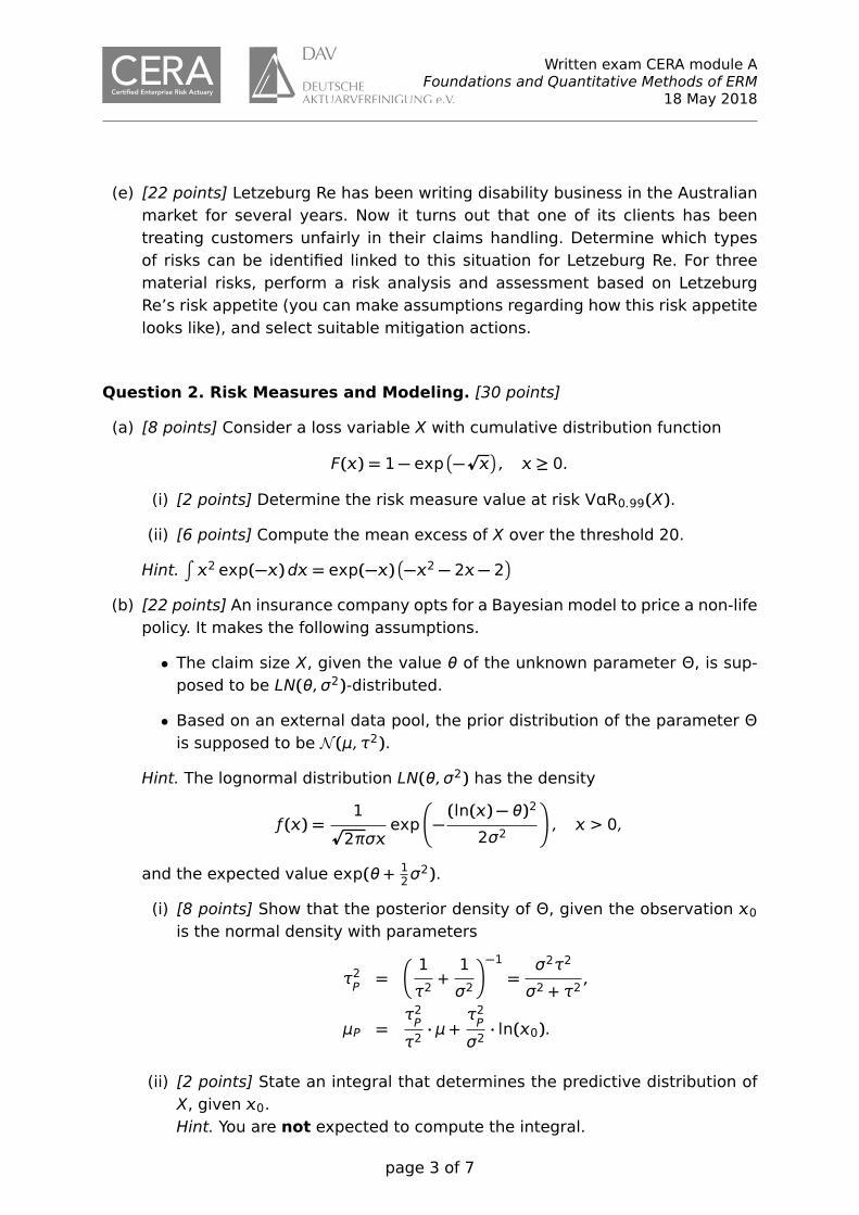
(e) [22 points] Letzeburg Re has been writing disability business in the Australianmarket for several years. Now it turns out that one of its clients has beentreating customers unfairly in their claims handling. Determine which typesof risks can be identified linked to this situation for Letzeburg Re. For threematerial risks, perform a risk analysis and assessment based on LetzeburgRe’s risk appetite (you can make assumptions regarding how this risk appetitelooks like), and select suitable mitigation actions.

Question 2. Risk Measures and Modeling. [30 points]

(a) [8 points] Consider a loss variable X with cumulative distribution function

F() = 1 − exp�

−p�

, ≥ 0.

(i) [2 points] Determine the risk measure value at risk VR0.99(X).

(ii) [6 points] Compute the mean excess of X over the threshold 20.

Hint.∫

2 exp(−)d = exp(−)�

−2 − 2 − 2�

(b) [22 points] An insurance company opts for a Bayesian model to price a non-lifepolicy. It makes the following assumptions.

• The claim size X, given the value θ of the unknown parameter Θ, is sup-posed to be LN(θ, σ2)-distributed.

• Based on an external data pool, the prior distribution of the parameter Θis supposed to be N (μ, τ2).

Hint. The lognormal distribution LN(θ, σ2) has the density

ƒ () =1

p2πσ

exp

�

−(ln() − θ)2

2σ2

�

, > 0,

and the expected value exp(θ + 12σ

2).

(i) [8 points] Show that the posterior density of Θ, given the observation 0is the normal density with parameters

τ2P=

�

1

τ2+1

σ2

�−1

=σ2τ2

σ2 + τ2,

μP =τ2P

τ2· μ +

τ2P

σ2· ln(0).

(ii) [2 points] State an integral that determines the predictive distribution ofX, given 0.Hint. You are not expected to compute the integral.

page 3 of 7


18 May 2018

(iii) [4 points] The predictive distribution from ii) turns out to be LN(μP, σ2+τ2P).Its expected shortfall is given by

ESα(X|0) =exp

�

μP + 0.5(σ2 + τ2P)�

1 − α· �Ç

σ2 + τ2P− −1(α)

�

,

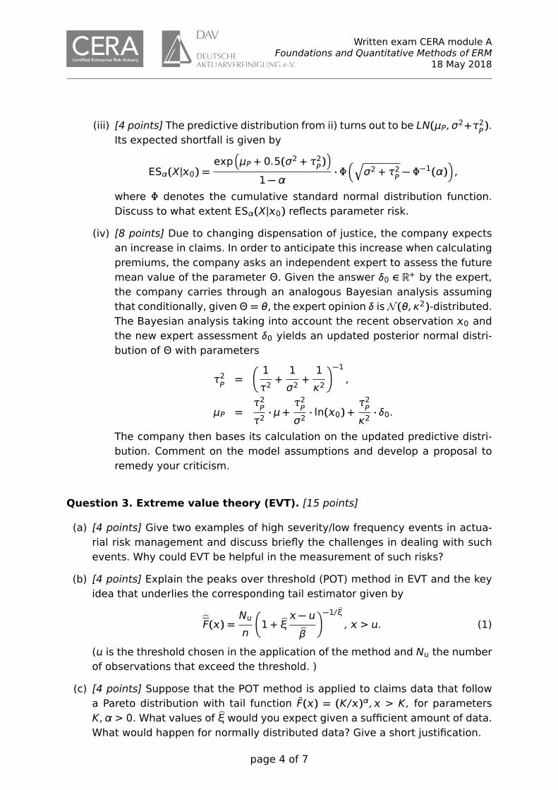
where denotes the cumulative standard normal distribution function.Discuss to what extent ESα(X|0) reflects parameter risk.

(iv) [8 points] Due to changing dispensation of justice, the company expectsan increase in claims. In order to anticipate this increase when calculatingpremiums, the company asks an independent expert to assess the futuremean value of the parameter Θ. Given the answer δ0 ∈ R+ by the expert,the company carries through an analogous Bayesian analysis assumingthat conditionally, given Θ = θ, the expert opinion δ is N (θ, κ2)-distributed.The Bayesian analysis taking into account the recent observation 0 andthe new expert assessment δ0 yields an updated posterior normal distri-bution of Θ with parameters

τ2P=

�

1

τ2+1

σ2+1

κ2

�−1

,

μP =τ2P

τ2· μ +

τ2P

σ2· ln(0) +

τ2P

κ2· δ0.

The company then bases its calculation on the updated predictive distri-bution. Comment on the model assumptions and develop a proposal toremedy your criticism.

Question 3. Extreme value theory (EVT). [15 points]

(a) [4 points] Give two examples of high severity/low frequency events in actua-rial risk management and discuss briefly the challenges in dealing with suchevents. Why could EVT be helpful in the measurement of such risks?

(b) [4 points] Explain the peaks over threshold (POT) method in EVT and the keyidea that underlies the corresponding tail estimator given by

b

F() =N

n

�

1 + bξ − bβ

�−1/ bξ

, > . (1)

( is the threshold chosen in the application of the method and N the numberof observations that exceed the threshold. )

(c) [4 points] Suppose that the POT method is applied to claims data that followa Pareto distribution with tail function F̄() = (K/)α, > K, for parametersK,α > 0. What values of bξ would you expect given a sufficient amount of data.What would happen for normally distributed data? Give a short justification.

page 4 of 7


18 May 2018

(d) [3 points] Suppose that the tail of an unknown loss distribution is modelled bythe tail estimator (1). Compute an estimator of VRα for α > 1 − N/N.

Question 4. Risk measures and capital allocation. [15 points] Consider aninsurance company with d business units. The loss of these units is described by therandom variables L, 1 ≤ ≤ d so that the total loss is given by L :=

∑d=1 L. Let ϱ by

a positively homogenous risk measure such as VRα or expected shortfall ESα, andlet ϱ(L) be the risk capital for the entire company. In this context a capital allocationprinciple allocates the capital AC1, . . . ,ACd to the individual business units, wherethe so-called full allocation property ϱ(L) =

∑d=1 AC has to hold.

(a) [4 points] Define for λ = (λ1, . . . , λd)′ the random variable L(λ) =∑d

=1 λL andlet rϱ(λ) = ϱ(L(λ)). Then the Euler capital allocation principle is given by

AC =∂rϱ

∂λ(1), 1 ≤ ≤ d.

Explain why capital allocation principles are used in risk adjusted performancemeasurement and discuss at least one economic argument that supports theuse of the Euler principle (simplicity and tractability are not enough).

b) [3 points] Consider a random variable L ∼ N(μ, σ2) and show that the expectedshortfall is given by

ESα(L) = μ + σφ(qα)

1 − α,

where φ denotes the density and qα the α quantile of the standard normaldistribution. Hint: it holds that

∫

e−2/2d = −e−2/2.

(b) [8 points] Expected shortfall contributions

(i) [6 points] Assume that (L1, . . . , Ld) are multivariate normal with meanμ = 0 and covariance matrix . Show that in this case the Euler capitalallocations for ϱ = ESα (the so-called expected shortfall contributions) aregiven by

AC =cov(L, L)p

vr(L)

φ(qα)

1 − α.

Hint: show using i) that ESα(∑d

=1 λL) = (λ′λ)1/2 φ(qα)1−α .

(ii) [2 points] State an alternative representation of the expected shortfallcontributions that holds generally (not only for elliptic distributions).

Question 5. Copulas and risk aggregation. [15 points] Consider an insurancecompany with two business lines and associated loss L1, L2. The company uses

page 5 of 7


18 May 2018

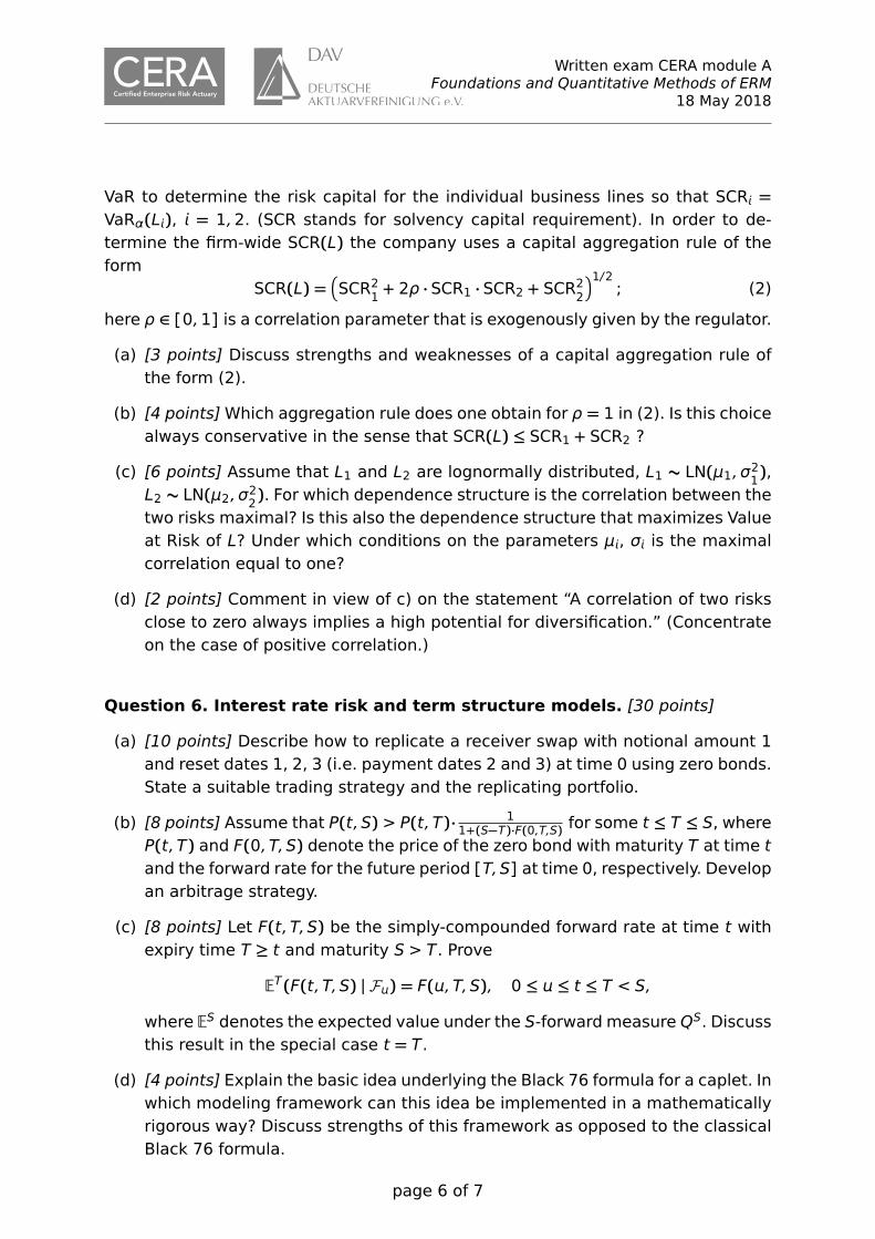
VaR to determine the risk capital for the individual business lines so that SCR =VaRα(L), = 1,2. (SCR stands for solvency capital requirement). In order to de-termine the firm-wide SCR(L) the company uses a capital aggregation rule of theform

SCR(L) =�

SCR21 + 2ρ · SCR1 · SCR2 + SCR22�1/2

; (2)

here ρ ∈ [0,1] is a correlation parameter that is exogenously given by the regulator.

(a) [3 points] Discuss strengths and weaknesses of a capital aggregation rule ofthe form (2).

(b) [4 points] Which aggregation rule does one obtain for ρ = 1 in (2). Is this choicealways conservative in the sense that SCR(L) ≤ SCR1 + SCR2 ?

(c) [6 points] Assume that L1 and L2 are lognormally distributed, L1 ∼ LN(μ1, σ21),L2 ∼ LN(μ2, σ22). For which dependence structure is the correlation between thetwo risks maximal? Is this also the dependence structure that maximizes Valueat Risk of L? Under which conditions on the parameters μ, σ is the maximalcorrelation equal to one?

(d) [2 points] Comment in view of c) on the statement “A correlation of two risksclose to zero always implies a high potential for diversification.” (Concentrateon the case of positive correlation.)

Question 6. Interest rate risk and term structure models. [30 points]

(a) [10 points] Describe how to replicate a receiver swap with notional amount 1and reset dates 1, 2, 3 (i.e. payment dates 2 and 3) at time 0 using zero bonds.State a suitable trading strategy and the replicating portfolio.

(b) [8 points] Assume that P(t, S) > P(t, T)· 11+(S−T)·F(0,T,S) for some t ≤ T ≤ S, where

P(t, T) and F(0, T, S) denote the price of the zero bond with maturity T at time tand the forward rate for the future period [T, S] at time 0, respectively. Developan arbitrage strategy.

(c) [8 points] Let F(t, T, S) be the simply-compounded forward rate at time t withexpiry time T ≥ t and maturity S > T. Prove

ET(F(t, T, S) | F) = F(, T, S), 0 ≤ ≤ t ≤ T < S,

where ES denotes the expected value under the S-forward measure QS. Discussthis result in the special case t = T.

(d) [4 points] Explain the basic idea underlying the Black 76 formula for a caplet. Inwhich modeling framework can this idea be implemented in a mathematicallyrigorous way? Discuss strengths of this framework as opposed to the classicalBlack 76 formula.

page 6 of 7


18 May 2018

Question 7. Risk management for corporate bonds and doubly stochastic

default times. [15 points] Consider a portfolio of corporate bonds in the assetportfolio of an insurer.

(a) [6 points] Describe the risks that affect this portfolio (at least 3 risk categories).Give an example of a risk that can be mitigated by using CDSs as a hedging in-strument, describe the corresponding strategy and mention ensuing problems.Describe another risk type that cannot be hedged with CDS.

(b) [9 points] Consider a single corporate zero-coupon bond with time to maturityT = 2 years and denote by τ the default time of the bond. The recovery valueof the bond is zero so that its payment at T is 1{τ>T} and the current price ofthe bond is p0.

Assume that the risk-free interest rate is equal to the constant r > 0, that underthe historical probability measure P, τ is doubly stochastic with hazard rateprocess γP and that under the risk-neutral measure Q, it is doubly stochasticwith hazard rate process γQ Moreover,

γPt= ψt and γQ

t= 2ψt

where ψ follows a CIR process with P-parameters κP, θP, σ > 0 and Q-parametersκQ, θQ, σ > 0.

(i) [4 points] Describe an algorithm to generate realization of the defaultindicator Yt = 1{τ≤t} under the historical measure P.

(ii) [5 points] Develop a simulation algorithm to compute the loss distributionand the VaR of the bond over the time horizon T = 1 year. Define for thisthe function

p(t1, t2, ψ; r, ρ, κ, θ, σ) = E�

exp�

−∫ t2

t1

r + ρψsds�

| ψt1 = ψ�

,

where ψ follows a CIR process with generic parameters κ, θ, σ. (Note thatp(t1, t2, ψ; r, ρ, κ, θ, σ) is known explicitly, but the precise form of this func-tion is not required). Explain, for which part of the simulation risk-neutralrespectively historical quantities are needed.

page 7 of 7

Proposal for solution to exam CERA module AFoundations and Quantitative Methods of ERM

18 May 2018

Proposal for solution

Question 1. Case study – Carrying out the role of CRO.

(a) Risk management is designed following the foundations of ERM by linking per-formance and systematic evaluation of risks and opportunities. More concre-tely, as first example specifically for a reinsurer it is important to anticipatethe clients are likely to be exposed and have a clear view of emerging risks.ERM thus provides early insights in business opportunities and a clear view onthe risk-return-relation. As second example, by our transparent and targetedcommunication throughout the group (e.g. quarterly risk report) we enhancerisk awareness but also bottom-up and top-down the information on opportu-nities. Thus, risk management creates value by avoiding losses, revealing op-portunities and allowing for risk-return-balanced decisions. At Letzeburg Re byrunning the internal model it is possible to analyse which business segmentsare profitable (creating at least the return that is necessary to serve the boundcapital) and which business segments are unprofitable. Also, it is possible toanalyse the diversification effect between business segments and betweenrisk categories. Possibilities for value creation are the support for underwritingprofitable business, the avoidance of unprofitable business and unwanted riskrealisations and the support of the value proposition from third parties. Thisincludes all aspects of qualitative risk management that are helping to main-tain and increase confidence in Letzeburg Re‘s value proposition. Example forsupporting profitable business: if only one of two treaties can be underwrittenbecause of capacity constraints use the internal model to find out which treatyis generating more value. Example for avoiding unwanted event realization:use natural catastrophe modeling to find out where limits for natural catastro-phe aggregates like US earthquakes or hurricanes should be set to avoid anundue exposure to the capital. Example for supporting the value proposition ofthird parties: demonstrate to analysts and rating agencies how effective yourun your operational risk management system.

(b) Shareholders are on the one hand interested in maximizing the return on theinvested capital with given (and transparent) risk and on the other hand mini-mizing of the risk for a given return (shareholder value approach). This impliesthe avoidance of over-capitalization i.e. hold capital buffers beyond the agreedrisk appetite. On the other hand this implies a risk-adequate capitalisation toavoid excessive risk for the invested capital. This implies a certain tension bet-ween short term maximisation of profit and long term stability. Letzeburg Re’sclients are interested in low premiums on the one hand and on the other handin financial stability of their reinsurer and easy claims handling. Regulators areinterested in protecting the policyholder and other beneficiaries and therefore

page 1 of 11


18 May 2018

look for capital standards and governance systems that assure a sufficient le-vel of protection. Return issues are of minor interest but efficient and effectiverisk management and conduct of business are considered as key elements ofproper governance. Different countries have different requirements. In orderto protect the value of Letzeburg Re it has to comply with Solvency II in Europe(Luxemburg and Ireland) and with the respective requirements in Bermuda,USA and Australia. For a reinsurer like Letzeburg Re it might be important tosafeguard a targeted rating. This is to protect the access to profitable businessas this is often ceded with rating constraints. Rating agencies have their ownvaluation systems with quantitative (mainly capital models) and qualitativerequirements. Capital models of rating agencies and internal models usuallydiffer as they are using different valuation approaches e.g. for diversification.Rating agencies as stakeholders follow their own business model as providerof information to investors, implying a certain ambition of achieving a uniqueselling point by own standards. Rating agencies action in the field of tensionof most transparent and valuable information for investors as clients and goodratings for rated companies also being clients. Management and staff of Letze-burg Re have a natural interest in protecting the value of the group as this willsafeguard their workplaces and income streams. The group´s strategy and riskstrategy are outlining how this can be achieved. Further stakeholders can be:Governments (e.g. stabilising the economy, protection against extreme eventsand protect tax streams), consultants and brokers (to earn fees by assisting inachieving business goals and compliance with external requirements) et.al.At publicly traded companies like Letzeburg Re a proposal to reflect differentvaluation systems simultaneously usually starts with shareholder value consi-derations which should find their way into the general strategy and the riskstrategy. All other valuation approaches are either mandatory (regulatory andaccounting requirements) or need a decision (targeted rating category) thatalso should be reflected in the strategy / risk strategy. In case of concurringrequirements (e. g. capital) the requirements need to be played out againsteach other depending on the situation. To give an example, comparing thesethree stakeholder groups, one finds that all are interested in financial stabilityof Letzeburg Re, but given their other interest to a different degree weight thisaspect. While shareholders would like to have an optimised minimum level ofcapital buffers, clients and supervisors would typically prefer a more comforta-ble capitalisation. Clients will also be interested in a good rating of LetzeburgRe as this will impact the credit risk they have to capitalise for. Letzeburg Rewill have to find the right balance.

(c) First proposal: Improvement of diversification between life & health and non-life. The current relation of 10 : 90 could be moved successively towards 50: 50 under the side condition, that life & health business are profitable andthe market allows for the expansion in that field. Correlation between these

page 2 of 11


18 May 2018

two business segments usually is very low. By using the internal model andworking with full probability distributions it might be possible to determinethe optimal business mix. Second proposal: When looking at potential expos-ures it appears that 50% of the non-life business comes from non-proportionalcatastrophe treaties. This appears to be quite high. A measure might be tomake better use of deferred tax assets and of the tax environments acrossthe company, e.g. Bermuda, to avoid the strain of money in „random“ goodyears that might be needed in „bad“ years („loss spread over time“). Thirdproposal: Diversification could be achieved by additional proportional non-catretail business with a less pronounced volatility and generate more stable cashflows. Fourth proposal: A reduction of natural catastrophe exposures by meansof cessions to third parties might improve the risk-return-relation and impro-ve relative return and stability. This can be done by traditional retrocessions toother insurers / reinsurers or by placements of these exposures into the capitalmarket (e. g. securitisations like CatBonds). The advantage of securitisationsis the availability of the liable capital and the option of diversification of coun-terparties, reducing credit risk. Fifth proposal: There are various possibilitiesto decrease the capital requirements of rating agencies. This usually turns outto be a direct value creation as rating agency capital requirements for upperrating categories tend to be significantly higher than respective requirementsfrom regulators or from internal models. S&P e.g. allows for approving theinternal model which then would enable Letzeburg Re to replace a certain per-centage of the overall capital requirement by the results of the internal model(„M-Factor“). The proposal therefore reads. Achieve / increase a positive M-Factor from Standard and Poor’s.

(d) (i) Possible „positive“ criteria are: positive working climate, transparency inobjective setting, definition of risk appetite etc, processes and communi-cation, open minded, behaviour of people in line with these criteria Pos-sible „negative“ criteria are: bureaucratism, formal approach, thinking insilos, „colleague viewed as a risk“, behaviour of people in line with thesecriteria

(ii) These criteria are all qualitative and like working climate at least hardor not directly measurable (con). To generate a rating nevertheless ERMculture has to be evaluated and is part of the rating as a measurement ofthe company. This could be checked and evaluated by looking at everydayaspects of decision making, at organisational and governance structurefor management of risks and communication of risk and risk managementand the degree of transparency of risk management processes includingtheir public communications (pro).

(e) Potential risks from this situation can be (a) insurance risk: additional claimspayments for past cases and higher claims for future cases, (b) credit risk:

page 3 of 11


18 May 2018

financial distress of the affected client with impact on the PV of future cashflows, (c) operational risk: internal control processes on “know your client”were insufficient and need to be reviewed, (d) legal/regulatory risk: fines forLetzeburg Re by the supervisor if they are found to be involved in the unfairtreatment, and (e) contagion risk: other clients may be found to have alsooperated unfairly, leading to higher claims with these clients as well and po-tentially reduced sales of disability products across the Australian market, (f)reputation risk: Letzeburg Re’s support of the unfair handling might impacton Letzeburg Re’s reputation in the Australian market, spreading to other mar-kets, (g) FX risk: payout of higher claims than expected in AUD might stress thecurrency hedging of the EUR balance sheet of the parent entity, (h) liquidityrisk: payout of higher claims than expected might stress the liquidity situationof the Australian subsidiary and require cash support from Letzeburg Re.

Risk analysis and assessment and mitigation – examples for (a) and (f)

(a) Insurance risk

Analysis: It can be expected that past cases which were refused by L’Re’sclient will be re-opened and settled in favour of the insureds, potentially inclu-ding accumulated claims payments. As the settlement practice of the insurerwill have to be revised in order to comply with the “treat customers fairly”approach, the rate of future claims is also expected to increase. As a conse-quence, reinsurance loss ratios under L’Re’s treaty for this client will increaseand are expected to be higher than assumed in best estimates and in pricing.

Assessment: Based on estimates from L’Re’s local claims department takinginto account the order of magnitude of fluctuations in annual disability claimsin the past years and the weight of the client in the overall portfolio, additio-nal claims due to the event for the current year are expected to be +4% oftotal volume, in absolute terms AUD 10m. Risk appetite for disability claimsdeviation is 5% in any year, so the risk is within the appetite.

Mitigation: The risk is with the appetite, so theoretically speaking the addi-tional claims payments could be accepted; but it would be better to enterinto negotiations with the client and to refuse the payment based on misbe-haviour and potential breach of contract. Best estimate for future claims andthe pricing need to be updated, new business premiums should also be re-negotiated. If the new claims expectations drive down the value of the deal tobelow target, and if the overall portfolio mix does allow for the associated lossof diversification benefit, it should be considered to terminate the relationshipwith the client.

(f) Reputation risk

page 4 of 11


18 May 2018

Analysis: The local management and strategy team sees that the close link inmedical underwriting and claims handling between reinsurer and cedant com-pany means that there is a high risk that L’Re’s reputation could be affected.This would not necessarily mean negative publicity in mainstream media, alt-hough this might also be the case, but primarily other insurance companiesin Australia and elsewhere could assume that L’Re was supporting the un-fair treatment, and refuse doing business with L’Re going forward. The impactwould be stronger for life and health, and weaker for non-life clients.

Assessment: Based on estimates from experts at L’Re’s parent entity and ta-king into account the total business volume of the company, loss of new busi-ness in the next year could be 5% of total life and health volume, and 1% ofnon-life premiums; in absolute terms EUR 0.5m and EUR 5m. This reflects thatthe relative lower impact on P&C translates into a higher absolute impact dueto the dominance in exposure. As L’Re is interested in a good rating it can beinferred that the risk appetite for reputational risk is very low and this event isa breach.

Mitigation: The risk needs to be reduced. L’Re should start a communicationcampaign to distance itself from the unfair treatment and to show active invol-vement in cooperating with industry bodies and supervisors in the clarificationand proper settlement of disputed claims. If the overall portfolio mix does al-low for the associated loss of diversification benefit, it should be considered toterminate the relationship with the client. To prevent the risk from re-occurring,L’Re should start client audits with the remaining disability clients to ensurethat their practices are sound.

Question 2. Risk Measures and Modeling.

(a) (i) Solving the equation 1 − exp(−p) = α gives the value at risk:

VRα(X) = (ln(1 − α))2.

We obtain VR0.99(X) = 21.21.

(ii) The mean excess over the threshold 20 is given by

E((X − 20)+) =∫ ∞

20( − 20) ·

1

2pexp(−

p)d

=∫ ∞

p20(y2 − 20) · exp(−y)dy

=∫ ∞

p20y2 exp(−y)dy − 20 · exp(−

p

20)

= [exp(−y)(−y2 − 2y − 2)]∞p20− 0.2285

= 0.1250.

page 5 of 11


18 May 2018

(b) (i) Up to a constant, the posterior density of Θ, given the observation 0 isgiven by

π(θ|0) ∝ ƒX(0|θ) · ƒΘ(θ)

∝ exp�

−1

2σ2(ln(0) − θ)2

�

· exp�

−1

2τ2(θ − μ)2

�

∝ exp�

−1

2σ2τ2�

(σ2 + τ2)θ2 − (2τ2 ln(0) + 2σ2μ)θ�

�

∝ exp

−1

2 σ2τ2

σ2+τ2

�

θ −τ2 ln(0) + σ2μ

σ2 + τ2

�2

.

Up to a constant, this is the density of N�

τ2 ln(0)+σ2μσ2+τ2 , σ2τ2

σ2+τ2

�

.

(ii) We obtain the predictive distribution of X by averaging the sample densityover the posterior density of the parameter.

ƒX(|0) =∫

ƒX(|θ) · π(θ|0)dθ

=∫ ∞

−∞

1p2π · σ

exp

�

−(ln() − θ)2

2σ2

�

·1

p2π · τP

exp

�

−(θ − μP)2

2 · τ2P

�

dθ

(iii) The predictive distribution from (ii) is given by LN(μP, σ2 + τ2P):

ƒX|0() =∫ ∞

−∞

1p2πσ

exp

�

−(ln() − θ)2

2σ2

�

·1

p2πτP

exp

�

−(θ − μP)2

2τ2P

�

dθ

=1

q

2π(τ2P+ σ2)

exp

�

−(ln() − μP)2

2(τ2P+ σ2)

�

·∫ ∞

−∞

q

τ2P+ σ2

p2πτPσ

exp

−τ2P+ σ2

2τ2Pσ2

�

θ −τ2Pln() + σ2μP

τ2P+ σ2

�2

dθ

=1

q

2π(τ2P+ σ2)

exp

�

−(ln() − μP)2

2(τ2P+ σ2)

�

, > 0

Its expected shortfall is given by

ESα(X|0) =exp

�

μP + 0.5(σ2 + τ2P)�

1 − α�Ç

σ2 + τ2P− −1(α)

�

,

where denotes the cumulative standard normal distribution function. Ifthe risk measure was calculated on the point estimate μP, we would obtainthe lower value

ESα(X) =exp

�

μP + 0.5σ2�

1 − α�p

σ2 − −1(α)�

.

The positive difference can be considered as measure of parameter risk.

page 6 of 11


18 May 2018

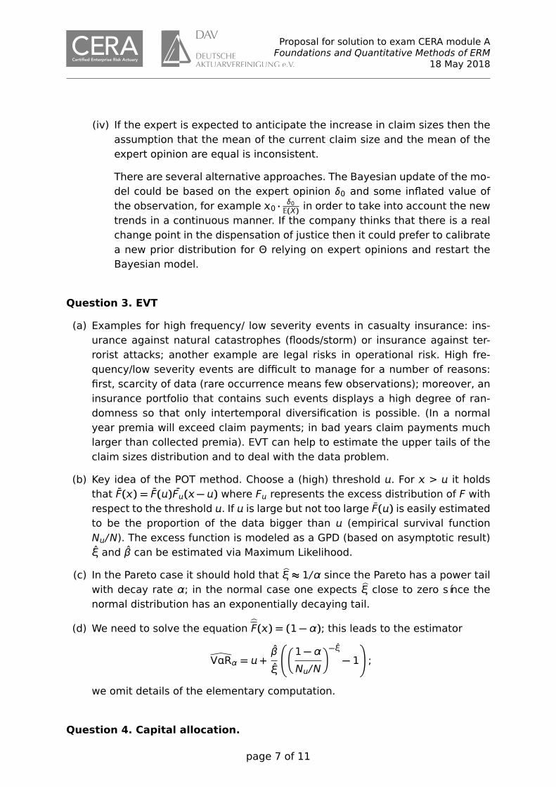
(iv) If the expert is expected to anticipate the increase in claim sizes then theassumption that the mean of the current claim size and the mean of theexpert opinion are equal is inconsistent.

There are several alternative approaches. The Bayesian update of the mo-del could be based on the expert opinion δ0 and some inflated value ofthe observation, for example 0 · δ0

E(X) in order to take into account the newtrends in a continuous manner. If the company thinks that there is a realchange point in the dispensation of justice then it could prefer to calibratea new prior distribution for Θ relying on expert opinions and restart theBayesian model.

Question 3. EVT

(a) Examples for high frequency/ low severity events in casualty insurance: ins-urance against natural catastrophes (floods/storm) or insurance against ter-rorist attacks; another example are legal risks in operational risk. High fre-quency/low severity events are difficult to manage for a number of reasons:first, scarcity of data (rare occurrence means few observations); moreover, aninsurance portfolio that contains such events displays a high degree of ran-domness so that only intertemporal diversification is possible. (In a normalyear premia will exceed claim payments; in bad years claim payments muchlarger than collected premia). EVT can help to estimate the upper tails of theclaim sizes distribution and to deal with the data problem.

(b) Key idea of the POT method. Choose a (high) threshold . For > it holdsthat F̄() = F̄()F̄(− ) where F represents the excess distribution of F withrespect to the threshold . If is large but not too large F̄() is easily estimatedto be the proportion of the data bigger than (empirical survival functionN/N). The excess function is modeled as a GPD (based on asymptotic result)ξ̂ and β̂ can be estimated via Maximum Likelihood.

(c) In the Pareto case it should hold that bξ ≈ 1/α since the Pareto has a power tailwith decay rate α; in the normal case one expects bξ close to zero sínce thenormal distribution has an exponentially decaying tail.

(d) We need to solve the equation b

F() = (1 − α); this leads to the estimator

ÖVRα = +β̂

ξ̂

�

1 − α

N/N

�−ξ̂

− 1

!

;

we omit details of the elementary computation.

Question 4. Capital allocation.

page 7 of 11


18 May 2018

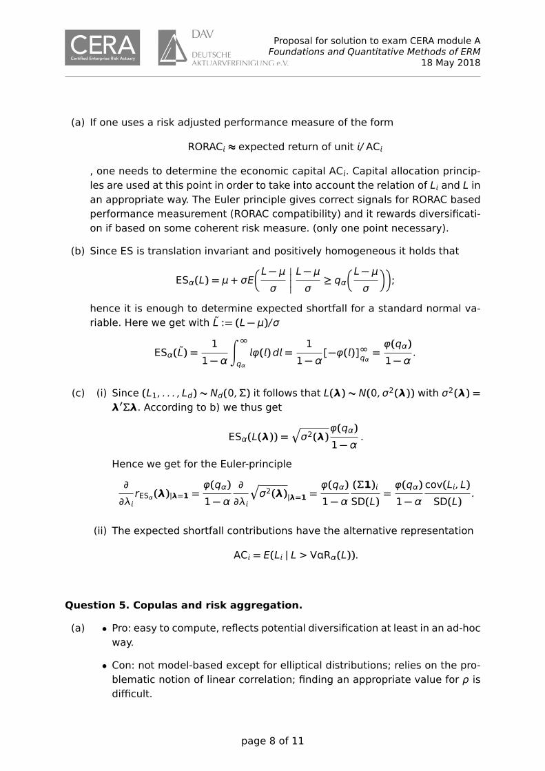
(a) If one uses a risk adjusted performance measure of the form

RORAC ≈ expected return of unit / AC

, one needs to determine the economic capital AC. Capital allocation princip-les are used at this point in order to take into account the relation of L and L inan appropriate way. The Euler principle gives correct signals for RORAC basedperformance measurement (RORAC compatibility) and it rewards diversificati-on if based on some coherent risk measure. (only one point necessary).

(b) Since ES is translation invariant and positively homogeneous it holds that

ESα(L) = μ + σE�L − μ

σ

�

�

�

�

L − μ

σ≥ qα

�L − μ

σ

��

;

hence it is enough to determine expected shortfall for a standard normal va-riable. Here we get with L̃ := (L − μ)/σ

ESα(L̃) =1

1 − α

∫ ∞

qα

φ()d =1

1 − α[−φ()]∞

qα=φ(qα)

1 − α.

(c) (i) Since (L1, . . . , Ld) ∼ Nd(0,) it follows that L(λ) ∼ N(0, σ2(λ)) with σ2(λ) =λ′λ. According to b) we thus get

ESα(L(λ)) =q

σ2(λ)φ(qα)

1 − α.

Hence we get for the Euler-principle

∂

∂λrESα(λ)|λ=1 =

φ(qα)

1 − α

∂

∂λ

q

σ2(λ)|λ=1 =φ(qα)

1 − α

(1)SD(L)

=φ(qα)

1 − α

cov(L, L)

SD(L).

(ii) The expected shortfall contributions have the alternative representation

AC = E(L | L > VRα(L)).

Question 5. Copulas and risk aggregation.

(a) • Pro: easy to compute, reflects potential diversification at least in an ad-hocway.

• Con: not model-based except for elliptical distributions; relies on the pro-blematic notion of linear correlation; finding an appropriate value for ρ isdifficult.

page 8 of 11


18 May 2018

(b) For ρ = 1 we obtain simple summation, SCR(L) = SCR1+ SCR2. This choice isnot conservative if we use VaR as risk measure; any counterexample to thesubadditivity of VaR is a counterexample. For ES simple summation would beconservative since ES is subadditive.

(c) According to Höffding’s theorem maximal correlation ρmax is attained if bothrisks are comonotonic. In that case it holds that VR(L1 + L2) = VR(L1) +VR(L2). This is in general not the maximal value of as VaR is not subadditive.It holds that ρmax = 1 if and only if both rvs are of the same type, that is forσ1 = σ2.

(d) The statement is in general not correct; depending on the choice of the mar-ginal distribution even comonotonic (perfectly dependent) risks may have lowlinear correlation (for instance two lognormal risks with very different σ). Thestatement is however correct for elliptical distributions.

Question 6. Interest rate risk and term structure models.

(a) Let K be the fixed rate. At time t = 0, we buy K shares of the zero bond withmaturity T = 2 and 1 + K shares of the zero bond with maturity T = 3 and sella zero bond with maturity T = 1. The price of this replicating portfolio is givenby

P = K · P(0,2) + (1 + K) · P(0,3) − P(0,1),

where P(t, T) denotes the price of the zero bond with maturity T at time t.

At time t = 1, we sell 1P(1,2) shares of the zero bond with maturity 2 in order to

pay one unit of currency to the holder of the zero bond that falls due at time 1.There remain K − 1

P(1,2) = K − L(1,2) − 1 shares of the zero bond with maturity2.

At time t = 2, the receiver swap pays the amount K − L(1,2). In order to settlethe remaining position of -1 unit of currency, we sell 1

P(2,3) shares of the zerobond with maturity 3. There remain

1 + K −1

P(2,3)= K − L(2,3)

shares of the zero bond with maturity 3, that pay the amount K − L(2,3) attime 3.

(b) At time t = 0 sell P(t,T)P(t,S) zero bonds with maturity S and buy 1 zero bond with

maturity T, resulting in a zero net investment. In addition, enter a receiverswap with K = F(t, T, S) and nominal 1 for free. At time T, the payment 1 of the

page 9 of 11


18 May 2018

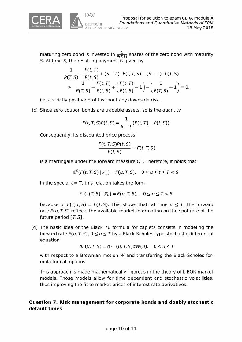
maturing zero bond is invested in 1P(T,S) shares of the zero bond with maturity

S. At time S, the resulting payment is given by

1

P(T, S)−P(t, T)

P(t, S)+ (S − T) · F(t, T, S) − (S − T) · L(T, S)

>1

P(T, S)−P(t, T)

P(t, S)+�

P(t, T)

P(t, S)− 1

�

−�

1

P(T, S)− 1

�

= 0,

i.e. a strictly positive profit without any downside risk.

(c) Since zero coupon bonds are tradable assets, so is the quantity

F(t, T, S)P(t, S) =1

S − T(P(t, T) − P(t, S)).

Consequently, its discounted price process

F(t, T, S)P(t, S)

P(t, S)= F(t, T, S)

is a martingale under the forward measure QS. Therefore, it holds that

ES(F(t, T, S) | F) = F(, T, S), 0 ≤ ≤ t ≤ T < S.

In the special t = T, this relation takes the form

ET(L(T, S) | F) = F(, T, S), 0 ≤ ≤ T < S.

because of F(T, T, S) = L(T, S). This shows that, at time ≤ T, the forwardrate F(, T, S) reflects the available market information on the spot rate of thefuture period [T, S].

(d) The basic idea of the Black 76 formula for caplets consists in modeling theforward rate F(, T, S), 0 ≤ ≤ T by a Black-Scholes type stochastic differentialequation

dF(, T, S) = σ · F(, T, S)dW(), 0 ≤ ≤ T

with respect to a Brownian motion W and transferring the Black-Scholes for-mula for call options.

This approach is made mathematically rigorous in the theory of LIBOR marketmodels. Those models allow for time dependent and stochastic volatilities,thus improving the fit to market prices of interest rate derivatives.

Question 7. Risk management for corporate bonds and doubly stochastic

default times

page 10 of 11


18 May 2018

(a) A portfolio of corporate bonds is affected among others by interest rate risk,spread risk (the risk of changes in credit spreads), default risk and the risk oflosses due to downgrading.

CDSs can be used to hedge default risk and - to a certain extent - credit risk.For this one would assume a protection buyer position in CDSs on the issuersof the bonds in the portfolio. Potential problems: basis risk (due to maturitymismatch and since CDSs are traded only for major bond issuers), counter-party risk (default of protection seller). Interest-rate risk cannot be hedged viaCDSs.

(b) (i) To simulate a realized trajectory of the default indicator Y = 1{τ≤t}, 0 ≤t ≤ T one would use threshold simulation as follows

1. Generate E ∼ Exp(1).

2. Generate a trajectory of ψ using P parameters κP, θP, σ up to T = 1 andcompute the integrated process P

t=∫ t

0 ψsds, t ≤ T.

3. If PT< E put Yt = 0 for 0 ≤ t ≤ T. Else let τ := inf{t ≥ 0 : Qt ≥ E} and

put Yt = 0 for t < τ and Yt = 1 for t ≥ τ.

(ii) We have the following algorithm to compute one realization of the lossassociated with the bond.

1. Generate a trajectory of ψ using P parameters κP, θP, σ up to T = 1.

2. Generate (for the trajectory from 1) a realisation of 1{τ>1} via thres-hold simulation (see i)

3. Return the loss

p0 − 1{τ>1}p(1,2, ψ1; r,1.5, κQ, θQ, σ)

Repeating this algorithm many times gives an approximation of the lossdistribution; from this the VaR can be computed by empirical quantile esti-mation.

page 10 of 10

tk

Textfeld

Page 11 of 11

Documents

Grundlagen und quantitative Methoden des ERM - aktuar.de · Schriftliche Prüfung CERA-Modul A Grundlagen und quantitative Methoden des ERM am 18.05.2018 Aufgabe 1. Fallstudie –