Heckscher Ohlin Handout

8/6/2019 Heckscher Ohlin Handout

http://slidepdf.com/reader/full/heckscher-ohlin-handout 1/13

Econ 340 Handout Heckscher-Ohlin-Samuelson Model Souvik Gupta

Production functions and properties of CRS production function:

• A production function shows the technically efficient relationship (no waste) between

the factor inputs, viz, labor (L) and capital (K) in our cases, and the output of a good.

Mathematically, a production function can be expressed as a functional relationship

between output (Y) and factor inputs as Y = f(L,K), where the function “f”summarizes the relationship. A few examples of production function are given below.

Fixed proportions

An important family of production functions which involves using the factor inputs in

fixed proportions. These production functions are also known as Leontief production

functions.

How can we describe such a technology precisely?

Y = min{L, K/2},

Check out the logic of this formula by considering the output it assigns to various

combinations of machines and workers:

1 labor and 2 machines yield min{1,2/2} = min{1,1} = 1 unit of output

2 labors and 4 machines yield min{2,4/2} = min{2,2} = 2 units of output

A general fixed proportions production function for two inputs has the form:

Y= min{aL,bK}, for some positive constants a and b.

Perfect substitutes

A technology whose character is exactly the opposite to that of a fixed proportions

technology and allows one input to be substituted freely for another at a constant rate.

We can describe the technology by the production function

Y = L + K

More generally, any production function of the form: Y = aL + bK, for any positive

constants a and b

A production function with smooth but not perfect substitution between inputs

Many technologies allow inputs to be substituted for each other, but not at a constant

rate. Suppose that one person operating a machine for an hour can produce 10 units of

Page 1 of 13




output using 10 units of raw material. If, for example, the speed of the machine isincreased, the same 10 units of output can be produced in 45 minutes using 15 units

of raw material, more raw materials being needed. If the speed is increased further,

the amount of raw material needed may increase by much more than 5 units.

A class of production functions that models situations in which inputs can besubstituted for each other to produce the same output, but cannot be substituted at a

constant rate, contains functions of the form:

Y = A.Lα K1-α , for some positive constants A and α, where 0< α <1

Such a production function is also known as a Cobb-Douglas production function.

An example of such a function is

Y = L1/2K1/2, where A = 1 and α = ½.

• We will assume for the discussion of Heckscher-Ohlin-Samuelson model that the

production function exhibits Constant Returns to Scale (CRS). By this it is meant that

if inputs are changed by certain proportion, then output also changes by the sameproportion. For example, in the Cobb-Douglas production function above, if L and K

are doubled, i.e. increased by 100%, then output also doubles.

• CRS production functions imply constant average cost of production in a perfectlycompetitive market structure, where firms do not have any pricing power.

• A constants average cost of production implies that marginal cost is also constant and

equal to the average cost. Thus, for CRS production functions under perfectcompetitions firms have AC = MC.

• Profit maximization by firms imply that marginal revenue should be equalized to

marginal cost. In the perfectly competitive market setup it becomes that price (which

is equal to marginal revenue for perfectly competitive firms) be equalized to marginalcost. So, a profit-maximizing firm with CRS technology and operating in a perfectly

competitive world, will always set P = MC.

• CRS production functions always exhibit positive marginal product (which is thechange in output per unit change in factor input usage) for the factor inputs. We shall

assume that, ceteris paribus, marginal products are decreasing: as more of one factorinput is added without changing the amount of the other factor input, then eachadditional unit of the former input produces less and less of output. However, if the

other factor input is allowed to vary as well, then marginal product of a factor input

may not exhibit decreasing returns.

• In the case of CRS production functions, the marginal product of a factor depends onthe ratio of factor inputs chosen.

Page 2 of 13




A higher (K/L) implies a higher marginal productivity for labor and a lower marginal

productivity for capital and vice-versa.

• A production process is called capital-intensive if it chooses a higher capital-labor

ratio at equilibrium. The equilibrium for a firm is defined as that particular inputcombinations which maximizes profit through cost minimization.

• One final property of the CRS production functions that is sometimes useful is the

“product exhaustion theorem”. This says that if each factor is paid an amount equal tothe value of its marginal product (i.e. price of the output multiplied by the marginal

product of the factor input), as would be the case if factor markets are perfectlycompetitive, then the revenue raised by selling the output will be just sufficient to pay

all factors of production leaving no room for any profit.

Decision making by a perfectly competitive firm with CRS production function:

L

K

X1

Y2

Y*

X*

O

KY

KX

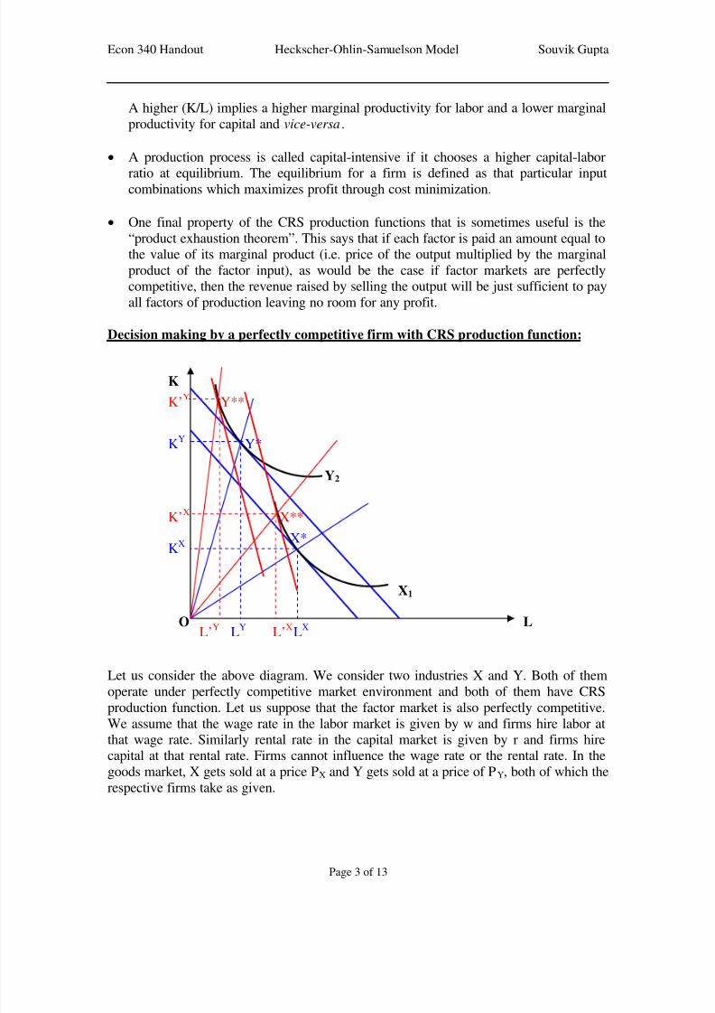
Let us consider the above diagram. We consider two industries X and Y. Both of them

operate under perfectly competitive market environment and both of them have CRS

production function. Let us suppose that the factor market is also perfectly competitive.We assume that the wage rate in the labor market is given by w and firms hire labor atthat wage rate. Similarly rental rate in the capital market is given by r and firms hirecapital at that rental rate. Firms cannot influence the wage rate or the rental rate. In the

goods market, X gets sold at a price PX and Y gets sold at a price of PY, both of which the

respective firms take as given.

LXLY

X**

Y**K’Y

K’X

L’Y L’X

Page 3 of 13




In the above diagram the negatively sloped line captures the cost of production. A singlesuch line (for example the blue solid line) represents a given total cost of production and

tells us various combinations of labor and capital that a firm can choose under the market

given wage and rental rates. For example, if w =10 and r = 5 and the firm wants to spend200, i.e. total cost = 200, then it can do so by choosing 10 units of L and 20 units of K or

by choosing 15 units of L and 10 units of K or by choosing 4 units of L and 32 units of Kand so on. For all these combinations of L and K the total cost of production is the same,viz. 200. That is why these negatively sloped lines are called isocost lines.

The further an isocost line is from the origin, the higher is the total cost of

production.

The slope of an isocost line is given by (w/r) preceded by a negative sign. So a

change in the (w/r) will change the slope. If (w/r) increases the isocost linesbecome steeper and if (w/r) falls isocost lines become flatter.

Similarly, in the above diagram we use isoquants for industry X and Y. Isoquants give usvarious combinations of L and K that produce the same amount of output. We have

shown one such isoquant for industry X and Y separately. Let us assume that the isoquant

labeled X1 implies lower output in X-industry than the isoquant labeled Y2 for Y-

industry.

Now, given the wage-rental ratio, and given the output level, a profit maximizing firm

will always try to minimize its cost of production. Thus it will seek to use thatcombination of L and K which can help the firm meet the output target at a minimum

cost. Diagrammatically, it means that given an isoquant a firm will seek to reach theisocost line which is closer to the origin, since closer to the origin implies lower cost of

production.

The profit maximizing equilibrium for each firm is obtained at the point of tangency

between an isoquant and an isocost line. This equilibrium is shown by X* for X-industry

and Y* for Y-industry. Notice, since Y industry has a higher output target than X-industry, its cost of production is also higher as given by an isocost line farther away

from the origin. But these two isocost lines are parallel as industries face the same (w/r).

At equilibrium, X industry chooses to employ OLX

units of labor and OKX

units of capital, whereas Y-industry chooses OLY units of labor and OKY units of capital. We can

see that at equilibrium, the capital-labor ratio (i.e. K/L) is higher for Y-industry. This can

be seen by drawing a ray from the origin through the equilibrium factor allocation point.The farther (nearer) the ray is from the horizontal axis, the more capital (labor) intensive

the production process is. In our example Y-industry in capital-intensive and it is easily

validated in the above diagram as the ray OY* is farther away from the horizontal axisthan the ray OX*.

Page 4 of 13




Formally, production of Y is capital intensive, if at equilibrium,

(KY / L

Y) > (K

X / L

X)

If industry Y is capital intensive, then it is mathematically true that industry X is laborintensive, i.e. (LY / K

Y) < (L

X / K

X)

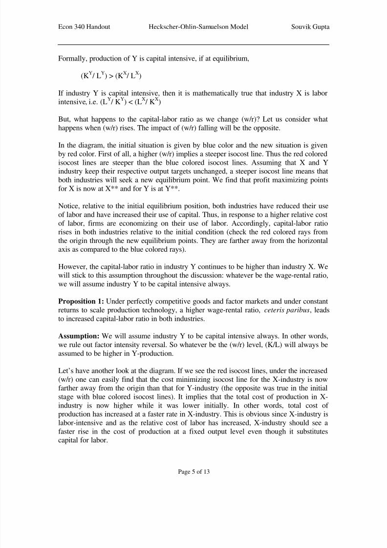
But, what happens to the capital-labor ratio as we change (w/r)? Let us consider what

happens when (w/r) rises. The impact of (w/r) falling will be the opposite.

In the diagram, the initial situation is given by blue color and the new situation is given

by red color. First of all, a higher (w/r) implies a steeper isocost line. Thus the red colored

isocost lines are steeper than the blue colored isocost lines. Assuming that X and Yindustry keep their respective output targets unchanged, a steeper isocost line means that

both industries will seek a new equilibrium point. We find that profit maximizing points

for X is now at X** and for Y is at Y**.

Notice, relative to the initial equilibrium position, both industries have reduced their use

of labor and have increased their use of capital. Thus, in response to a higher relative cost

of labor, firms are economizing on their use of labor. Accordingly, capital-labor ratiorises in both industries relative to the initial condition (check the red colored rays from

the origin through the new equilibrium points. They are farther away from the horizontal

axis as compared to the blue colored rays).

However, the capital-labor ratio in industry Y continues to be higher than industry X. Wewill stick to this assumption throughout the discussion: whatever be the wage-rental ratio,

we will assume industry Y to be capital intensive always.

Proposition 1: Under perfectly competitive goods and factor markets and under constant

returns to scale production technology, a higher wage-rental ratio, ceteris paribus, leads

to increased capital-labor ratio in both industries.

Assumption: We will assume industry Y to be capital intensive always. In other words,

we rule out factor intensity reversal. So whatever be the (w/r) level, (K/L) will always be

assumed to be higher in Y-production.

Let’s have another look at the diagram. If we see the red isocost lines, under the increased

(w/r) one can easily find that the cost minimizing isocost line for the X-industry is nowfarther away from the origin than that for Y-industry (the opposite was true in the initial

stage with blue colored isocost lines). It implies that the total cost of production in X-

industry is now higher while it was lower initially. In other words, total cost of production has increased at a faster rate in X-industry. This is obvious since X-industry is

labor-intensive and as the relative cost of labor has increased, X-industry should see a

faster rise in the cost of production at a fixed output level even though it substitutescapital for labor.

Page 5 of 13




Since the output target has remained unchanged, a faster rise in the total cost of

production in X-industry implies that the average cost of production has also increased at

a faster rate in X-industry. Now, under CRS production function, we know average costof production equals marginal cost production, which in turn equals to the product price

under perfectly competitive market structure. A faster rise in the average cost of production in X-industry following a rise in (w/r), thus, implies that the relative price of good X, viz. (PX /PY), also goes up.

Proposition 2: Under perfectly competitive goods and factor markets and under constant

returns to scale production technology, a higher wage-rental ratio, ceteris paribus, leadsto higher relative price for the labor intensive production process.

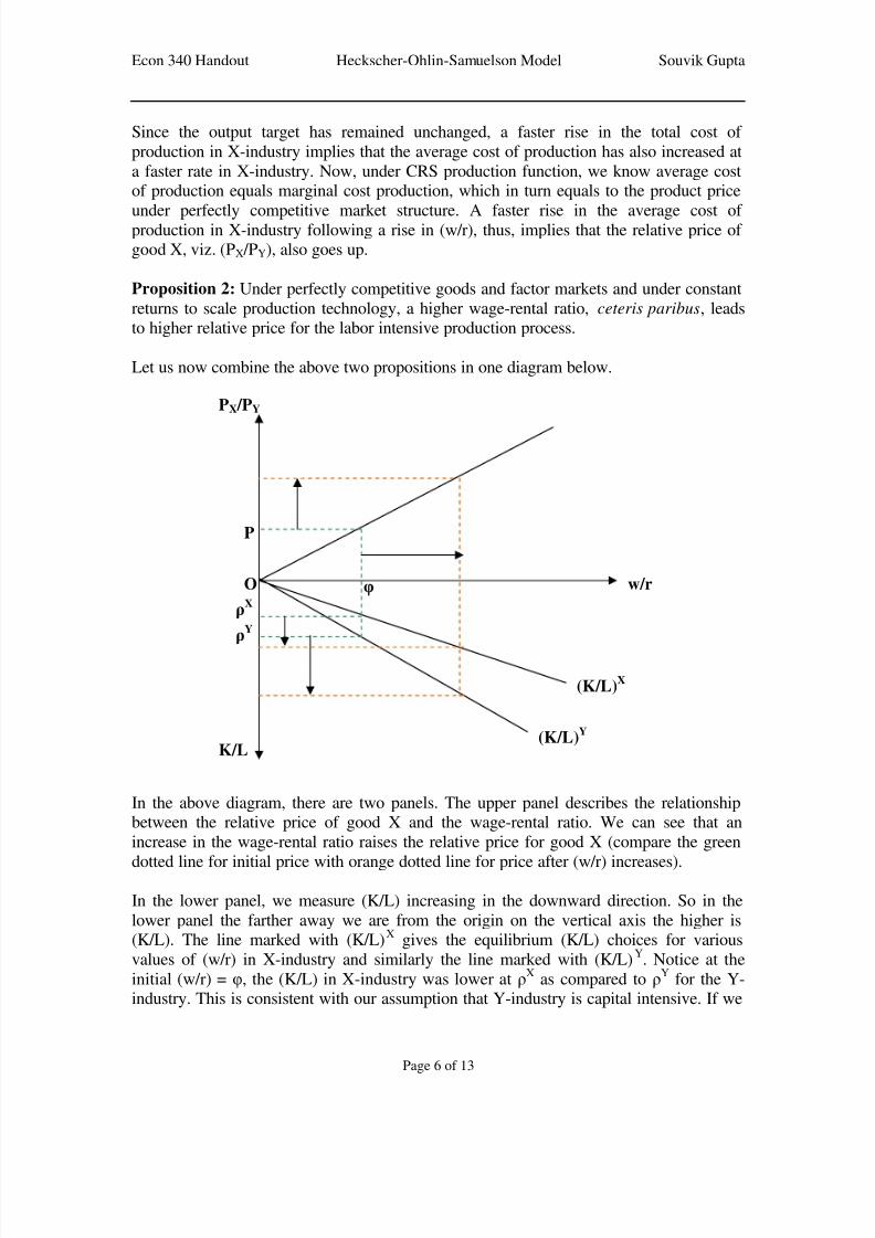
Let us now combine the above two propositions in one diagram below.

w/r

PX /PY

K/L

O

(K/L)X

P

ρX

ρY

φ

(K/L)Y

In the above diagram, there are two panels. The upper panel describes the relationshipbetween the relative price of good X and the wage-rental ratio. We can see that an

increase in the wage-rental ratio raises the relative price for good X (compare the green

dotted line for initial price with orange dotted line for price after (w/r) increases).

In the lower panel, we measure (K/L) increasing in the downward direction. So in the

lower panel the farther away we are from the origin on the vertical axis the higher is(K/L). The line marked with (K/L)X gives the equilibrium (K/L) choices for various

values of (w/r) in X-industry and similarly the line marked with (K/L)Y. Notice at the

initial (w/r) = φ, the (K/L) in X-industry was lower at ρX

as compared to ρY

for the Y-industry. This is consistent with our assumption that Y-industry is capital intensive. If we

Page 6 of 13




increase (w/r), the (K/L) for both industries rise (compare the green and orange dottedlines for each industry separately). However, the (K/L) in Y-industry is still higher than

that in X-industry, which is consistent with our assumption that there is no factor-

intensity reversal.

Now, we are ready for the discussion of the Heckscher-Ohlin-Samuelson model after allthese build-ups.

Heckscher-Ohlin-Samuelson Model:

Assumptions:

1. There are 2 countries, 2 commodities and 2 factors of production (2x2x2 model).

2. There is perfect competition in both goods and factor markets.3. All production functions exhibit constant returns to scale.

4. The production functions are such that two commodities show different factor

intensities at a common factor price ratio, but there is no factor intensity reversal.5. Production functions differ between commodities, but they are identical in both

countries.

6. Factors of production are perfectly mobile between industries within a country,

but perfectly immobile between countries.7. Taste and consumer preferences are identical in the two countries.

8. Whenever these two countries engage in trade, it will be considered as free trade.

The assumption that the two countries have identical production technologies in X and Y

productions (assumption 5 above) and that perfect competition prevails everywhereensure that we can use the same diagram for both the countries to describe the

relationship between relative price and wage-rental ratio and also factor-intensity and

wage-rental ratio.

The two countries will, however, be different in terms of their endowment of labor and

capital. Thus, the countrywide capital-labor ratio is assumed to vary between the twocountries in this model. We will call the countries A and B. Based on the endowments of

capital and labor, we need to find out the factor abundance in these countries.

Definitions:

Physical definition of factor abundance:

Country B is called capital-rich if (K/L)B > (K/L)A

Notice, these capital-labor ratios are at the country level and they relate to the relativefactor abundance at the country level. The capital-labor ratio at the industry level defines

the factor intensity and it is assumed that X-industry is always labor-intensive in both the

countries and Y-industry is always capital-intensive in both the countries. Factor intensityin production is different from factor abundance for a country.

Page 7 of 13




Price definition of factor abundance:

Country B is called a capital-rich country if at autarky , (w/r)B

> (w/r)A.

In a two country setup, if a country is capital-rich, then it is mathematically true that theother country is labor-rich.

In our example, we will always assume country A to be labor-rich and country B to be

capital-rich.

Typically, these two definitions are same under the assumption that tastes and consumer

preferences are identical in the two countries (assumption 7). Without this assumption

these two definitions of factor abundance could have different implications. We rule outany possibility of divergence between the two definitions with the help of assumption 7.

The theorem:

Under the above set of assumptions, the Heckscher-Ohlin theorem states that a capital-

rich country will have comparative advantage in the capital-intensive good and a labor-

rich country will have comparative advantage in labor-intensive good.

So, now we have one possible answer to the question how a country attains comparative

advantage in some lines of production. But we should also keep in mind that this is notthe only possible reason for the existence of comparative advantage.

If we, now, appeal to the theory of comparative advantage, we know that a country

exports the good in which it has a comparative advantage. Hence, by combining the

Heckscher-Ohlin theorem and theory of comparative advantage we can say a capital-rich(labor-rich) country will have comparative advantage in the capital-intensive good (labor-

intensive good), will also export the capital-intensive good (labor-intensive good) and

will import the labor-intensive good (capital-intensive good).

(Continued….)

Page 8 of 13




Free Trade and Factor Rewards in the Heckscher-Ohlin-Samuelson model:

w/r

PX /PY

K/L

O

(K/L)

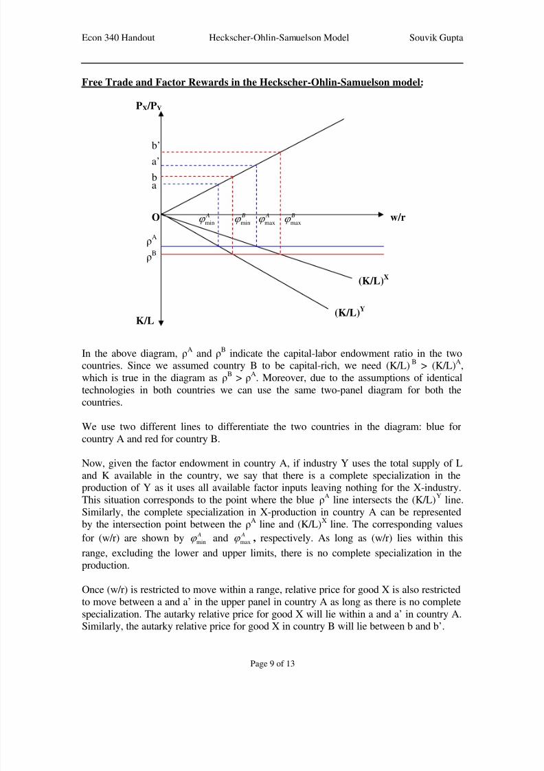
In the above diagram, ρA

and ρB

indicate the capital-labor endowment ratio in the twocountries. Since we assumed country B to be capital-rich, we need (K/L)B > (K/L)A,

which is true in the diagram as ρB > ρ

A. Moreover, due to the assumptions of identical

technologies in both countries we can use the same two-panel diagram for both the

countries.

We use two different lines to differentiate the two countries in the diagram: blue for

country A and red for country B.

Now, given the factor endowment in country A, if industry Y uses the total supply of L

and K available in the country, we say that there is a complete specialization in theproduction of Y as it uses all available factor inputs leaving nothing for the X-industry.

This situation corresponds to the point where the blue ρA line intersects the (K/L)Y line.

Similarly, the complete specialization in X-production in country A can be representedby the intersection point between the ρ

A line and (K/L)X line. The corresponding values

for (w/r) are shown by min

A

ϕ and max

A

ϕ , respectively. As long as (w/r) lies within thisrange, excluding the lower and upper limits, there is no complete specialization in the

production.

Once (w/r) is restricted to move within a range, relative price for good X is also restricted

to move between a and a’ in the upper panel in country A as long as there is no complete

specialization. The autarky relative price for good X will lie within a and a’ in country A.Similarly, the autarky relative price for good X in country B will lie between b and b’.

X

(K/L)Y

a

ρA

ρB

min

Aϕ

a’

b

b’

min

B max

Bϕ ϕ max

Aϕ

Page 9 of 13




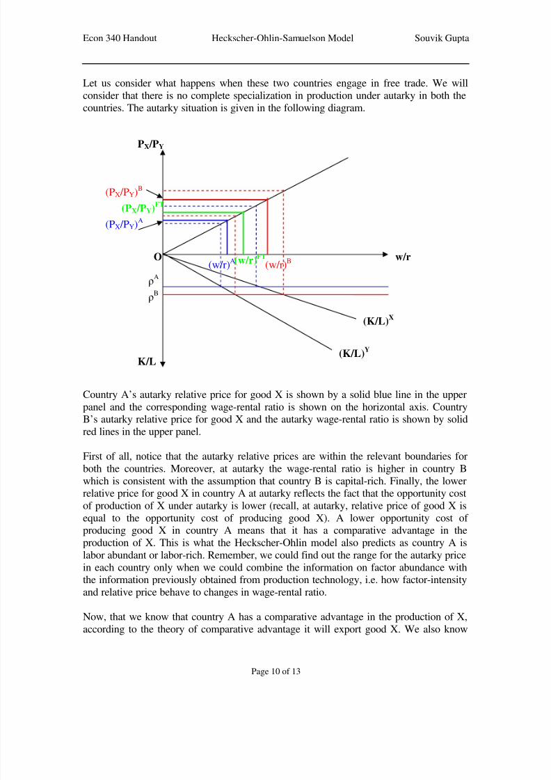
Let us consider what happens when these two countries engage in free trade. We will

consider that there is no complete specialization in production under autarky in both the

countries. The autarky situation is given in the following diagram.

w/r

PX /PY

K/L

O

(K/L)X

(K/L)Y

ρA

ρB

(PX /PY)A

(PX /PY)B

Country A’s autarky relative price for good X is shown by a solid blue line in the upper

panel and the corresponding wage-rental ratio is shown on the horizontal axis. CountryB’s autarky relative price for good X and the autarky wage-rental ratio is shown by solid

red lines in the upper panel.

First of all, notice that the autarky relative prices are within the relevant boundaries for

both the countries. Moreover, at autarky the wage-rental ratio is higher in country B

which is consistent with the assumption that country B is capital-rich. Finally, the lowerrelative price for good X in country A at autarky reflects the fact that the opportunity cost

of production of X under autarky is lower (recall, at autarky, relative price of good X is

equal to the opportunity cost of producing good X). A lower opportunity cost of producing good X in country A means that it has a comparative advantage in the

production of X. This is what the Heckscher-Ohlin model also predicts as country A islabor abundant or labor-rich. Remember, we could find out the range for the autarky price

in each country only when we could combine the information on factor abundance withthe information previously obtained from production technology, i.e. how factor-intensity

and relative price behave to changes in wage-rental ratio.

Now, that we know that country A has a comparative advantage in the production of X,

according to the theory of comparative advantage it will export good X. We also know

(w/r)A (w/r)B

(PX /PY)FT

(w/r)FT

Page 10 of 13




that in order to induce the producers of good X in country A to export to the country B,they need to be given a price incentive in the form of a higher world relative price for

good X. We also know that the world relative price for good X will lie between its

autarky relative prices in the two country. So, we pick a price in between the two autarkyprices and represent it with solid green line. The free trade variables are shown with a

“FT” superscript.

Weak form of factor price equalization:

Under the assumptions of the Heckscher-Ohlin-Samuelson model and with no complete

specialization, free trade in goods and services leads to equalization in the relative returnsto the factors of production in the two countries.

This is one of the important predictions of the Heckscher-Ohlin-Samuelson model. It isimportant because we see equalization of relative return to factor inputs across

international borders even though factors are completely immobile internationally. This is

happening because under free trade relative prices of goods are equalized to theirrespective world market prices and through that channel relative return to labor is

converging to (w/r)FT in both countries separately. Please remember that there is no

international factor market. This equalization in the relative return is happening due to the

relationship between the product prices and factor prices in each country.

We can see that under free trade the relative price of good X rises in country A and falls

in country B. At the same time the relative return to labor, viz (w/r), in country A alsorises and falls in country B. So, in country A, labor gains relative to capital and in country

B labor loses relative to capital.

The opposite is happening to the relative return to capital, which is given by (r/w). As

country B exports the capital intensive good Y, the relative price of Y in country B rises(falls in country A) and relative return to capital in country B rises (falls in country A).

Strong form of factor price equalization:

Under the assumptions of the Heckscher-Ohlin-Samuelson model and with no complete

specialization, free trade in goods and services leads to equalization in the real returns to

the factors of production in the two countries.

The only difference between the weak and strong form of factor price equalization (FPE)

is that the former talks about the relative return to factor inputs and the latter talks aboutreal returns to factor inputs.

Real return to labor in terms of good X is given by: w/PX

Real return to labor in terms of good Y is given by: w/PY

Real return to capital in terms of good X is given by: r/PX

Real return to capital in terms of good X is given by: r/PY

Page 11 of 13




We know that (w/r) rises in country A after free trade. So, a move from autarky to freetrade will make firms economize on their use of labor in both industries and they will, in

fact, increase the (K/L) in both industries under free trade. Since both industries exhibit

CRS in their production technology, higher (K/L) during free trade implies marginalproductivity of labor rises and that of capital falls in both industries.

We also know from microeconomic theory, real return to factor inputs under perfectlycompetitive factor market is equal to their marginal product. Thus, in country A higher

marginal product for labor under free trade in the production of both X and Y means a

higher real return to labor in terms of both the goods. On the other hand, under free trade

real return to capital decreases under free trade in country A in terms of both the goods.

In country B, (w/r) falls, i.e. (r/w) rises, under free trade. Thus both industries will

economize on their use of capital and will reduce their (K/L). Hence, the marginalproductivity of labor falls in both industries leading to fall in real returns in terms of both

the goods. On the other hand, a fall in (K/L) leads to an increase in the marginal

productivity of capital in both the industries under free trade and its real return rises interms of both the goods.

Finally, since both countries use the same technology they will be choosing the same

(K/L) in X-industry while facing the (w/r)* and same (K/L) in Y-industry. Thus,marginal productivity of labor and capital in X-industry will be the same in both the

countries, which means that real returns in terms of good X will also be the same.

Similarly, marginal productivity of labor and capital will be the same in Y-industry inboth the countries implying equalization of real returns between the countries in terms of

good Y as well.

Hence, not only relative returns to factors of production are equalized, real returns are

also equalized between the countries.

Note: in the presence of complete specialization and/or widely apart factor endowments

for the two countries, even though free trade will lead to equalization in the relativeprices for the goods in the two countries, there will be no factor price equalization.

Stolper-Samuelson Theorem:

The above discussion leads us to the Stolper-Samuelson theorem. We could see earlier

that due to free trade relative price of the export good rises in both the countries, and it

was the factor used intensively in the production of the export good that saw a rise in therelative return and also a rise in the real return in each country.

Stolper-Samuelson theorem links this movement in product prices to factor returns. Itsays that under the assumptions of CRS production functions, full-employment of factors

and perfectly competitive market a rise in the relative price, ceteris paribus, of a good

leads to an increase in the return to the factor input used intensively in the production of that good and a drop in the return to the other factor input.

Page 12 of 13




In the above discussion of the Heckscher-Ohlin-Samuelson model we saw that a rise in

the relative price of good X under free trade leads to an increase to the return to labor in

country A. Similarly, return to capital in country B rises as the price of the capital-intensive good Y rises under free trade.

Rybczynski Theorem:

If the endowment of one of the factor input increases under full-employment, ceteris

paribus, the output of the good using this factor intensively rises and that of the other

good, which does not use this factor intensively, falls.

Thus, if there is a rise in labor endowment in our example, everything else remaining the

same, there will be a rise in the production of X and a drop in the production of Y.

Page 13 of 13

Documents

Heckscher Ohlin Handout