Embed Size (px)
Citation preview
TECHNISCHE UNIVERSITÄT MÜNCHEN
Lehrstuhl „Economics of Aging“
REFORMS, INCENTIVES AND FLEXIBILIZATION
Five Essays on Retirement
Nicolas Goll
Vollständiger Abdruck der von der Fakultät für Wirtschaftswissenschaften der
Technischen Universität München zur Erlangung des akademischen Grades eines
Doktors der Volkswirtschaft (Dr. oec. publ.) genehmigten Dissertation.
Vorsitzender: Prof. Dr. Robert K. Freiherr von Weizsäcker
Prüfer der Dissertation:
1. Prof. Dr. Axel Börsch-Supan, Ph.D.
2. Prof. Regina T. Riphahn, Ph.D., Friedrich-Alexander-Universität Erlangen-Nürnberg
Die Dissertation wurde am 24.02.2020 bei der Technischen Universität München eingereicht und
durch die Fakultät für Wirtschaftswissenschaften am 15.05.2020 angenommen.


To my parents

Acknowledgements
This dissertation would not have been possible without the support of many people who
accompanied me along the way. I would like to use this occasion to express my gratitude for their
support.
First, I would like to thank Prof. Dr. h.c. Axel Börsch-Supan, Ph.D. for giving me the chance to
work in such a stimulating environment like the MEA in Munich. I am thankful for his support and
the comments on my work. I am in particular grateful for the tremendously instructive
collaborations through the time of writing this dissertation and for the opportunity to always work
on the most current policy issues. Furthermore, I would like to thank Prof. Regina Riphahn, Ph.D.
who agreed to be the second examiner of this dissertation and to Prof. Dr. Robert Frhr. von
Weizsäcker for being the chairperson of my dissertation committee.
Over the last nearly five years, many people at MEA have contributed to the success of this work.
I am in particular grateful to Prof. Dr. Tabea Bucher-Koenen for her great support and confidence
from the very beginning. Tabea is co-author of the fourth chapter. Furthermore, I would like to
thank Dr. Irene Ferrari and Dr. Johannes Rausch especially for their great collaboration in the
International Social Security Project. The collaboration and the conferences have always been
engaging and led to the second and third chapter of this dissertation. Moreover, I am thankful to
Dr. Vesile Kutlu Koc for being my first mentor and for co-authoring the fourth chapter. I also would
like to thank all of my research assistants, in particular Elisabeth Gruber, Hannah Horton and
Christina Meyer, for their excellent assistance over the last years. A special thanks goes to
Dr. Sebastian Kluth for initially bringing my attention to MEA. Last but not least, very special
thanks go to Dr. Felizia Hanemann and Dr. Klaus Härtl without whom working at MEA would not
have been as much fun.
However, above all, I would like to thank my wife Dr. Ricarda Zeh, LL.M. (Columbia) and my
parents. Without their love and unconditional support, not only over the last years but throughout
my whole life, I would not have been able to get to the point where I am now, let alone finish my
dissertation. This dissertation is dedicated to my parents.
v
Contents
List of abbreviations ....................................................................................................................... x
List of figures ................................................................................................................................. xi
List of tables .................................................................................................................................. xv
1. Reforms, Incentives and Flexibilization: General Introduction ......................................... 1
1.1 Social Security Reforms and the Changing Retirement Behavior in Germany ................. 8
1.2 Retirement Decisions in Germany: Micro-Modelling ....................................................... 9
1.3 Dangerous Flexibility – Retirement Reforms Reconsidered ........................................... 10
1.4 Dangerous Flexible Retirement Reforms – A Supplementary Placebo Analysis across Time ...................................................................................................................... 11
1.5 Working Pensioners in Europe ........................................................................................ 12
1.6 Closing Remarks.............................................................................................................. 13
2. Social Security Reforms and the Changing Retirement Behavior in Germany .............. 16
2.1 Introduction ..................................................................................................................... 16
2.2 Employment rate among older individuals and pension claiming behavior .................... 18
2.3 Institutional changes: German pension policy and its development ............................... 25
2.3.1 German pension system until 1980 .......................................................................... 25
2.3.2 Reform process since 1980 ...................................................................................... 28
2.3.2.1 Phase 1 (1980 to 1992): modest retrenchment within the pension system/increasing generosity outside the pension system ................... 29
2.3.2.2 Phase 2 (1992 to 2007): sustainability reforms................................................. 29
2.3.2.3 Phase 3 (2007 to 2016): reform backlash, the “pension with 63” .................... 35
Contents
vi
2.4 The implicit tax on working longer ................................................................................. 40
2.4.1 Definition ................................................................................................................. 40
2.4.2 Empirical implementation ........................................................................................ 41
2.5 Results ............................................................................................................................. 46
2.5.1 Replacement rates and social security wealth, scaled for Germany ......................... 46
2.5.1.1 Replacement rate ............................................................................................... 46
2.5.1.2 Social security wealth ....................................................................................... 49
2.5.2 Common macro environment: replacement rates, social security wealth and its accrual ................................................................................................................. 51
2.5.2.1 Replacement rate ............................................................................................... 51
2.5.2.2 Social security wealth ....................................................................................... 52
2.5.2.3 Accrual rates ..................................................................................................... 53
2.5.3 Common macro environment: implicit taxes on working longer............................. 55
2.5.4 Implicit taxes on working longer by education/skill ................................................ 62
2.5.5 German macro environment: the influence of changes in the taxation, cohort-specific income profiles and survival probabilities .................................................. 63
2.5.6 Relation between implicit taxes and employment rates ........................................... 65
2.5.7 Relation between implicit taxes and pension claiming ages .................................... 67
2.6 Conclusions ..................................................................................................................... 70
3. Retirement Decisions in Germany: Micro-Modelling ....................................................... 71
3.1 Introduction ..................................................................................................................... 71
3.2 German public pension system ........................................................................................ 74
3.3 Data and variable specification ........................................................................................ 79
3.3.1 The German Socio-Economic Panel ........................................................................ 79
3.3.2 Income profiles ......................................................................................................... 81
3.3.3 Definition of retirement status .................................................................................. 83
3.4 The implicit tax on working longer ................................................................................. 87
3.5 Validation of pension calculator ...................................................................................... 91
3.6 Expected pension benefits on multiple pathways to retirement ...................................... 94

Contents
vii
3.7 Results ............................................................................................................................. 96
3.7.1 ITAX based on micro data ....................................................................................... 96
3.7.2 Empirical estimation ................................................................................................ 97
3.7.2.1 The retirement model ........................................................................................ 97
3.7.2.2 Estimation results .............................................................................................. 99
3.8 Counterfactual simulations ............................................................................................ 104
3.9 Conclusions ................................................................................................................... 110
4. Dangerous Flexibility – Retirement Reforms Reconsidered ........................................... 111
4.1 Introduction ................................................................................................................... 111
4.2 Labor supply and retirement patterns ............................................................................ 113
4.3 Flexibility reforms ......................................................................................................... 116
4.4 Economic theory: More flexibility does not necessarily increase labor supply ............ 120
4.4.1 A simple model of a stylized flexibility reform ..................................................... 121
4.4.2 Model extensions and pension policy .................................................................... 123
4.5 Empirical analysis.......................................................................................................... 127
4.5.1 Methodology .......................................................................................................... 127
4.5.2 Data ........................................................................................................................ 128
4.5.3 Pooled OLS ............................................................................................................ 131
4.5.4 Synthetic control method ....................................................................................... 134
4.5.4.1 The model ....................................................................................................... 134
4.5.4.2 Treatment effects ............................................................................................ 135
4.6 Conclusions ................................................................................................................... 144
5. Dangerous Flexible Retirement Reforms – A Supplementary Placebo Analysis
across Time .......................................................................................................................... 147
5.1 Introduction ................................................................................................................... 147
5.2 The synthetic control method ........................................................................................ 150
5.2.1 The model ............................................................................................................... 150
5.2.2 Requirements and limitations of the synthetic control method .............................. 152

Contents
viii
5.2.3 Inference with the synthetic control method: in-space placebos and in-time placebos ..................................................................................................... 153
5.3 Data and variables ......................................................................................................... 156 5.4 Results ........................................................................................................................... 158
5.4.1 Labor force participation ........................................................................................ 159
5.4.2 Working hours ........................................................................................................ 165
5.4.3 Total labor supply .................................................................................................. 170
5.5 Summary and conclusion ............................................................................................... 174
6. Working Pensioners in Europe .......................................................................................... 176
6.1 Introduction ................................................................................................................... 176
6.2 Economic theory and institutional details ..................................................................... 179
6.3 Data and variables ......................................................................................................... 185
6.3.1 SHARE data and other data ................................................................................... 185
6.3.2 Variables and sample selection .............................................................................. 185
6.4 Empirical analysis.......................................................................................................... 192
6.4.1 Part I: within-country variation .............................................................................. 192
6.4.1.1 Regression analysis ......................................................................................... 192
6.4.1.2 Variance decomposition ................................................................................. 196
6.4.2 Part II: between-country variation.......................................................................... 198
6.5 Summary and conclusions ............................................................................................. 202
A. Appendix to Chapter 4 ....................................................................................................... 204
A.1 Flexible retirement options and institutional details ...................................................... 204
A.2 Mathematical appendix to model of stylized flexibility reform .................................... 207
A.3 Descriptive statistics ...................................................................................................... 210
A.4 Checking for changes in trend ....................................................................................... 212
A.5 Pre- and post-treatment periods by country ................................................................... 213
A.6 Synthetic control weights .............................................................................................. 214
A.7 Robustness of the treatment effects ............................................................................... 216
A.8 The quality of pre-treatment characteristics .................................................................. 219

Contents
ix
B. Appendix to Chapter 5 ....................................................................................................... 223
B.1 Pre- and post-treatment periods by country ................................................................... 223
B.2 Synthetic control weights .............................................................................................. 224 B.3 Robustness of the treatment effects ............................................................................... 226
B.4 Quality of pre-treatment characteristics......................................................................... 228
B.5 Sensitivity check: dropping Luxembourg from the synthetic control groups ............... 231
C. Appendix to Chapter 6 ....................................................................................................... 238
References ................................................................................................................................... 249

x
List of abbreviations
AEA Average exit age
DC Defined contribution
DB Defined benefit
DRV Deutsche Rentenversicherung Bund
EEA Earliest eligibility age
EP Earnings points
FRA Full rate age
GDP Gross domestic product
GRV Gesetzliche Rentenversicherung
GSOEP German Socio-Economic-Panel
ISSP International Social Security Project
ITAX Implicit tax on working longer
LFP Labor force participation
NBER National Bureau of Economic Research
OECD Organization for Economic Co-operation and Development
PAYG Pay-as-you-go
pp(s) Percentage point(s)
SEA Statutory eligibility age
SHARE Survey of Health, Ageing and Retirement in Europe
SSW Social security wealth
SUF Scientific use file
TLS Total labor supply
VSKT Versichertenkontenstichprobe
WH Working hours
xi
List of figures
Figure 1.1: West German employment rate by age group and gender ............................................. 2
Figure 2.1: West German employment rate by age group and gender ........................................... 17
Figure 2.2: West Germany older women’s employment rate with and without correction for general trend in younger women’s employment rates .................................................................... 20
Figure 2.3: Average pension claiming age by gender (West Germany) ........................................ 21
Figure 2.4: Coverage of pathways to retirement on annual newly claimed pensions .................... 22
Figure 2.5: Pension claiming by age and year (1985-2015) in West Germany ............................. 23
Figure 2.6: Timeline of the reforms to the social security system ................................................. 28
Figure 2.7: Eligibility ages with and without actuarial deductions for each pathway to retirement in respect to legal situation ............................................................................................................. 38
Figure 2.8: (Synthetic) Earnings profiles by gender and education ............................................... 43
Figure 2.9: Coverage of pathways to retirement on annual newly claimed pensions without passively insured individuals .......................................................................................................... 45
Figure 2.10: Replacement rate for median educated men, women and couples by age ................. 47
Figure 2.11: Average replacement rate of age group 60-64 by education group ........................... 48
Figure 2.12: Median educated men’s, women’s and couple’s social security wealth of leaving the labor market immediately in 1,000€ by age ................................................................ 49
Figure 2.13: Average social security wealth of age group 60-64 in 1,000€ by education ............. 50
Figure 2.14: Replacement rate for median educated men, women and couples by age (common case) ............................................................................................................................... 51
Figure 2.15: Average replacement rate of age group 60-64 by education group (common case) ............................................................................................................................... 52
Figure 2.16: Median educated men’s, women’s and couple’s social security wealth of leaving the labor market immediately in 1,000€ by age (common case) ....................................... 52
List of figures
xii
Figure 2.17: Average social security wealth of age group 60-64 in 1,000€ by education (common case) ............................................................................................................................... 53
Figure 2.18: Median educated men’s, women’s and couple’s accrual of social security wealth of leaving the labor market immediately in 1,000€ by age (common case) ................................... 54
Figure 2.19: Average accrual of social security wealth of age group 60-64 in 1,000€ by education (common case) ............................................................................................................... 54
Figure 2.20: Median educated men’s implicit taxes over time by age ........................................... 58
Figure 2.21: Median educated men’s implicit taxes by age ........................................................... 59
Figure 2.22: Median educated women’s implicit taxes over time by age ...................................... 60
Figure 2.23: Median educated women’s implicit taxes by age ...................................................... 60
Figure 2.24: Median educated couple’s implicit taxes over time ................................................... 61
Figure 2.25: Median educated couple’s implicit taxes by age ....................................................... 61
Figure 2.26: Implicit taxes aggregated over age 60 to 64 by education group .............................. 62
Figure 2.27: Average implicit taxes (of ages 60 to 64) for common and German taxation ........... 64
Figure 2.28: Average implicit taxes (of ages 60 to 64) for common and German cohort-specific income profiles and survival probabilities ..................................................................................... 65
Figure 2.29: Employment rate versus implicit tax ......................................................................... 66
Figure 2.30: Development of single person’s implicit tax and pension claiming at different ages .................................................................................................................................. 69
Figure 3.1: West German employment rate by age group and gender ........................................... 72
Figure 3.2: Pathways to retirement, West Germany....................................................................... 77
Figure 3.3: Earnings points profiles by gender and education ....................................................... 82
Figure 3.4: Earnings points flat profiles by gender and education ................................................. 83
Figure 3.5: Retiring, benefit claiming and flexible retirement ....................................................... 84
Figure 3.6: Working status and benefit claiming by age and gender ............................................. 85
Figure 3.7: Retirement hazard by gender ....................................................................................... 86
Figure 3.8: Distance between husband and wife’s retirement dates by age difference .................. 87
List of figures
xiii
Figure 3.9: ITAX in Germany over time by single years of age, men, median-educated .............. 89
Figure 3.10: ITAX in Germany over time by single years of age, women, median-educated ....... 90
Figure 3.11: Validation of pension benefit calculator – Distribution of predicted vs. observed pension benefits by age groups and pension type .......................................................................... 92
Figure 3.12: Validation of pension benefit calculator – Difference between predicted and observed pensions by age group and pension type ......................................................................... 93
Figure 3.13: Distribution of ITAX by age ...................................................................................... 96
Figure 3.14: Counterfactual simulation: average retirement probability for age 55-65 ............... 105
Figure 3.15: Counterfactual simulation: average retirement probability for age 55-59 ............... 106
Figure 3.16: Counterfactual simulation: average retirement probability for age 60-65 ............... 106
Figure 3.17: Counterfactual simulation: percentage of individuals still working at age 65 ......... 107
Figure 3.18: Observed labor force participation of men, age group 55-69, 1984-2015 ............... 108
Figure 3.19: Counterfactual simulation: expected retirement age at age 55 ................................ 109
Figure 3.20: Counterfactual simulation: expected retirement age at age 62 ................................ 109
Figure 4.1: Labor force participation rate (LFPR) by single years of age, statutory eligibility age (SEA) and average exit age (AEA) by country, 2012, males ................................................ 115
Figure 4.2: Number of hours worked when middle-aged ............................................................. 122
Figure 4.3: Number of hours worked when young (a) and total number of life-time hours worked (b) .......................................................................................................................... 125
Figure 4.4: Trends in labor force participation: treated vs. synthetic control .............................. 136
Figure 4.5: Trends in working hours: treated vs. synthetic control .............................................. 138
Figure 4.6: Trends in males’ total labor supply: treated vs. synthetic control ............................. 141
Figure 5.1: Trends in labor force participation: treated vs. synthetic control. Actual reform years ...................................................................................................................... 160
Figure 5.2: Trends in labor force participation: treated vs. synthetic control. Placebo reform years .................................................................................................................... 161
Figure 5.3: Trends in working hours: treated vs. synthetic control. Actual reform years ............ 165
Figure 5.4: Trends in working hours: treated vs. synthetic control. Placebo reform years .......... 166
List of figures
xiv
Figure 5.5: Trends in total labor supply: treated vs. synthetic control. Actual reform year ......... 170
Figure 5.6: Trends in total labor supply: treated vs. synthetic control. Placebo reform year ....... 171
Figure 6.1: Working pensioner proportion across countries ........................................................ 187
Figure 6.2: Potential determining factors of being a working pensioner ......................................... 193
Figure 6.3: Variance decomposition for the probability of being a working pensioner ............... 196
Figure 6.4: Counterfactual simulation for working pensioner proportions .................................. 199
Figure A.7.1: Trends in males’ LFP aged 55-64, robustness of the treatment effects ................. 217
Figure A.7.2: Trends in males’ working hours aged 55-64, robustness of the treatment effects ........................................................................................................................... 218
Figure B.3.1: Trends in males’ LFP aged 55-64, robustness of the treatment effects. Placebo reform year ...................................................................................................................... 227
Figure B.3.2: Trends in males’ working hours aged 55-64, robustness of the treatment effects. Placebo reform year ...................................................................................................................... 228
Figure B.5.1: Trends in males’ LFP aged 55-64: treated vs. synthetic control. Placebo reform years. Without Luxembourg in the synthetic control groups .............................. 233
Figure B.5.2: Trends in males’ working hours aged 55-64: treated vs. synthetic control. Placebo reform years. Without Luxembourg in the synthetic control group ............................... 234
Figure B.5.3: Trends in males’ total labor supply aged 55-64: treated vs. synthetic control. Placebo reform years. Without Luxembourg in the synthetic control group ............................... 235
Figure B.5.4: Trends in males’ LFP aged 55-64, robustness of the treatment effects. Placebo reform year. Without Luxembourg in the synthetic control group ................................. 236
Figure B.5.5: Trends in males’ working hours aged 55-64, robustness of the treatment effects. Placebo reform year. Without Luxembourg in the synthetic control group ................................. 237
Figure C.1: Depiction of potential mismeasurement .................................................................... 238
Figure C.2: Potential determining factors of being a working pensioner. Based on linear regression model ........................................................................................................................... 238
Figure C.3: Counterfactual simulation for working pensioner proportions. Based on linear regression model ........................................................................................................................... 238
xv
List of tables
Table 2.1: Pathways to retirement. Eligibility criteria ................................................................... 26
Table 2.2: Standard net replacement rate and standard net replacement rate before taxes ............ 27
Table 2.3: Unemployment benefits as percentage of last net income ............................................ 33
Table 2.4: Contribution to public pension system for unemployed as percentage of last gross income ............................................................................................................................ 34
Table 2.5: Maximal duration time of unemployment benefits for older workers in months ......... 36
Table 2.6: Actuarial adjustment factor for early/late pension claiming in percentage by pathway to retirement, pension claiming age and cohort/pension claiming year ........................... 37
Table 3.1: Pathways to retirement. Eligibility criteria ................................................................... 76
Table 3.2: Descriptive statistics of main variables ......................................................................... 81
Table 3.3: Regression estimates for single households (accrual rate) .......................................... 100
Table 3.4: Regression estimates for couple households (accrual rate) ......................................... 100
Table 3.5: Regression estimates for single households (ITAX) ................................................... 100
Table 3.6: Regression estimates for couple households (ITAX) .................................................. 101
Table 3.7: Regression estimates for single households using alternative models (accrual rate) ................................................................................................................................. 102
Table 3.8: Regression estimates for couple households using alternative models (accrual rate) ................................................................................................................................. 102
Table 3.9: Regression estimates for single households using alternative models (ITAX) ........... 103
Table 3.10: Regression estimates for couple households using alternative models (ITAX) ........ 103
List of tables
xvi
Table 4.1: Effects of flexibility reforms on labor force participation (LFP), working hours and total labor supply (TLS) ............................................................................................................... 132
Table 4.2: Post-treatment results regarding LFP of males aged 55-64, effects and pseudo p-values ............................................................................................................................ 137
Table 4.3: Post-treatment results regarding working hours of males aged 55-64, effects and pseudo p-values ............................................................................................................................ 140
Table 4.4: Post-treatment results for total labor supply of males aged 55-64, effects and pseudo p-values ............................................................................................................................ 142
Table 5.1: Post-treatment results regarding LFP of males aged 55-64, effects and pseudo p-values ............................................................................................................................ 162
Table 5.2: Post-treatment results regarding working hours of males aged 55-64, effects and pseudo p-values ............................................................................................................................ 168
Table 5.3: Post-treatment results for total labor supply of males aged 55-64, effects and pseudo p-values ............................................................................................................................ 172
Table 6.1: Overview of institutional details concerning flexible retirement options and earnings tests ................................................................................................................................ 182
Table 6.2: Summary statistics ...................................................................................................... 191
Table A.1.1: Overview of flexible retirement options, earnings tests and mandatory retirement regulations across countries .......................................................................................................... 205
Table A.3.1: Descriptive statistics ................................................................................................ 210
Table A.4.1: OLS Regression – effects of flexibility reforms on labor force participation (LFP), working hours and total labor supply (TLS) – trend specification ............................................... 212
Table A.5.1: Treated countries and time periods for labor force participation (LFP) and working hours (WH) .................................................................................................................... 213
Table A.6.1: Synthetic control weights, outcome variable: labor force participation .................. 214
Table A.6.2: Synthetic control weights, outcome variable: weekly working hours ..................... 215
Table A.8.1: Labor force participation predictor means before the partial retirement reform ..... 220
Table A.8.2: Working hours predictor means before the partial retirement reform ..................... 221
List of tables
xvii
Table B.1.1: Treated countries, placebo reform years and time periods for labor force participation (LFP) and working hours (WH) .............................................................................. 223
Table B.2.1: Synthetic control weights, outcome variable: Labor force participation ................. 224
Table B.2.2: Synthetic control weights, outcome variable: weekly working hours ..................... 225
Table B.4.1: Labor force participation predictor means before the flexibility reform ................. 229
Table B.4.2: Working hours predictor means before the flexibility reform ................................. 230
Table B.5.1: Post-treatment results regarding LFP of males aged 55-64, effects and pseudo p-values. Without Luxembourg in the synthetic control group ....................................... 233
Table B.5.2: Post-treatment results regarding working hours of males aged 55-64, effects and pseudo p-values. Without Luxembourg in the synthetic control group ....................................... 234
Table B.5.3: Post-treatment results regarding total labor supply of males aged 55-64, effects and pseudo p-values. Without Luxembourg in the synthetic control group ....................................... 235
Table C.1: Gross domestic product and labor force participation rate of age group 55–64 by countries ....................................................................................................................................... 239
Table C.2: Sample size, gender composition and average age by group and country ................. 239
Table C.3: Potential determining factors of working pensioners. Dependent variable: working pensioner yes/no ........................................................................................................................... 240
Table C.4: Potential determining factors of working pensioners. Dependent variable: working pensioner yes/no ........................................................................................................................... 242
Table C.5: Potential determining factors of working pensioners. Dependent variable: working pensioner yes/no. Based on linear regression model .................................................................... 242

xviii
1
1. Reforms, Incentives and Flexibilization: General Introduction
Demographic change is one megatrend of the twenty-first century.1 Demographic change holds the
potential for substantial social, political and economic change around the world throughout the next
decades. Most industrialized countries currently undergo such a change in demographic patterns
which is mainly caused by two developments: First, life expectancy has substantially risen in almost
all parts of the world. Second, low fertility rates have evolved since the 1970s, even if there is some
variation across countries. Both developments taken together have led to aging populations in many
countries. At the same time, the average retirement age in industrialized countries declined
throughout most of the twentieth century. In combination, these developments put enormous
pressure on pension systems, many of which have proven to be financially unsustainable. In
particular, an aging population jeopardizes Pay-as-you-go (PAYG) pension systems where the
contributions of current employees finance pension benefits of current pensioners. This has caused
a long-lasting debate on how to make old-age provision systems more sustainable (see e.g. Gruber
and Wise 1999, 2004). Most governments in developed countries have implemented fundamental
pension reforms in order to stabilize the pension systems.2
Germany is in particular confronted with demographic change. While life expectancy is constantly
increasing, the country experienced an extraordinary sequence of large birth cohorts born in the
second half of the 1950s and the 1960s (baby boomers) and subsequent low fertility rates since the
1970s.The slightly increasing birthrates in the last years will overall not be able to counteract
1 John Naisbitt, a futurologist and best-selling author, coined the term megatrend for long-term processes of transformation with a broad scope and a fundamental impact. See, e.g., Naisbitt (1982) and Naisbitt and Aburdene (1990). 2 The extent of those large reform efforts around the globe are for instance described in the country chapters in Börsch-Supan and Coile (2019) presenting in great detail the reform process in 12 Western industrialized countries over the past almost four decades. Besides, Barr and Diamond (2010) give an introduction to the economics of pension reforms.
1. General Introduction
2
population aging. Moreover, the baby boomers will reach eligibility ages for pension benefits over
the next years, which leads to one million individuals more retiring within the next five years in
comparison to the last five years. Already in the near future, this will dramatically change the ratio
between the working age population and pension benefit recipients. However, there will not be
demographic easing in the longer run either: The old-age dependency ratio – the number of
individuals aged 65 and over per 100 people in the working age (aged 20 to 64) – will almost double
from 35.3 in 2015 to 65.1 in 2050 (OECD 2015).
The German public pension system (Gesetzliche Rentenversicherung) is organized as PAYG
system and features a very broad coverage. About 85% of the German workforce are part of the
system.3 For most insurants pension benefits from the public pension system form the most
important source of income in old age. Therefore, the financial imbalance of the public pension
system is particularly alarming.
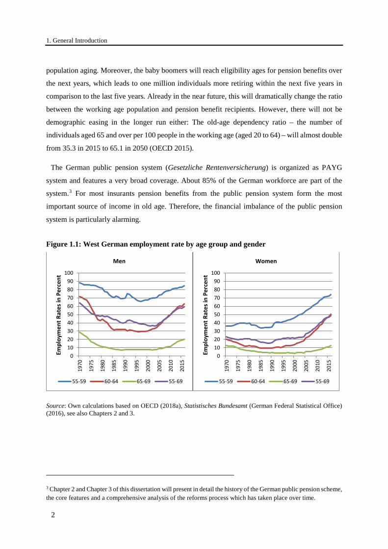
Figure 1.1: West German employment rate by age group and gender
Source: Own calculations based on OECD (2018a), Statistisches Bundesamt (German Federal Statistical Office) (2016), see also Chapters 2 and 3.
3 Chapter 2 and Chapter 3 of this dissertation will present in detail the history of the German public pension scheme, the core features and a comprehensive analysis of the reforms process which has taken place over time.
0102030405060708090
100
1970
1975
1980
1985
1990
1995
2000
2005
2010
2015
Empl
oym
ent R
ates
in P
erce
nt
Men
55-59 60-64 65-69 55-69
0102030405060708090
100
1970
1975
1980
1985
1990
1995
2000
2005
2010
2015
Empl
oym
ent R
ates
in P
erce
nt
Women
55-59 60-64 65-69 55-69

1. General Introduction
3
While demographic change has constantly continued in Germany, working later in life has been
undergoing a remarkable change throughout the last decades (see Figure 1.1). The employment rate
of older men experienced a long declining trend that began in the early 1970s. Since about 2000,
employment rates of both older men and older women have been stunningly increasing. For males,
the overall picture shows a U-shaped pattern with a reversal at the end of the 1990s. The
employment rates of women aged 55 to 59 experienced a rather constant increase and a mild reversal
for the older age groups. Whether the recent increase in employment rates of older workers can help
to permanently reduce the negative consequences of aging on fiscal sustainability depends on
whether the trend will continue. Consequently, it is important to understand the causes for this
recent increase.
Promising candidates for an explanation of the trend reversal are secular developments like
younger cohorts with improved health and better education, and the different role of women in
society. However, previous literature has shown that these developments have contributed
surprisingly little (Coile et al. 2019 for an overview; Börsch-Supan and Ferrari 2019 for Germany).
Hence, the causes of the trend reversal have to be found elsewhere. Another promising explanatory
factor could be found in institutional changes such as reforms of the pension system. After the
pension reforms in Germany in the 1960s and 1970s had led to one of the world’s most generous
public pension systems, the acknowledgement of demographic change initiated a series of reforms
meant to foster the sustainability of the system in times of demographic pressure. The most
important reform measures aiming at more sustainability were:
• Introduction of actuarial adjustment factors for early retirement
• Increase of eligibility ages for drawing pension benefits
• Abolishment of pathways to early retirement
• Introduction of a self-regulating factor in the pension adjustment formula that links the
benefits to the system’s dependency ratio (“sustainability factor”)
• Introduction of flexible retirement options
Recently, however, the reform process toward a sustainable public pension system ended and
Germany experienced a phase of reform backlashes. “Bridges to early retirement” outside the public
pension system were strengthened and new and generous early retirement options inside the public
pension system were created which already have led to behavioral responses. For instance, the 2014
reform increased the generosity of a specific early retirement pathway for individuals with long
insurance careers by reducing the eligibility age for full pension benefits from 65 to 63 (“retirement

1. General Introduction
4
at 63”). The reform aimed at individuals who have worked in burdensome employment for many
years (Deutscher Bundestag 2014). Dolls and Krolage (2019) showed that individuals who are
eligible for the generous early retirement pathways claim benefits on average 5.4 months earlier
than non-eligible individuals with identical characteristics. Moreover, they illustrated that the
reform involves enormous additional costs for the pension system.4
This dissertation aims at investigating the role of structural policy changes in explaining the
employment trend reversal of older individuals. The reforms have constantly altered the incentives
to stay in the labor force and to claim pension benefits, respectively. The first central objective of
the dissertation is to analyze how these reforms have influenced retirement incentives over time and
consequently, whether they have set the stage for increasing employment rates. The second aim is
to investigate how much of the German trend reversal in employment rates later in life can be
attributed to these varying retirement incentives. This eventually reflects the collective effect of the
many reforms.
Turning away from the conglomeration of reforms and focusing on one specific reform device,
the third central aim of the dissertation is to examine the role of flexibilization in connection to
retirement choices and labor supply decisions of older individuals. Not only in Germany but also in
other countries flexible retirement options have been enacted as part of reform processes. The idea
of flexible retirement is to insert a transition period with reduced work effort between the phases of
full-time employment and full retirement. The income loss resulting from the work reduction is
supposed to be compensated by drawing (partial) pension benefits or by other compensatory sources
(e.g. governmental subsidies, unemployment insurance funds, occupational pension funds etc.).
One objective of flexibilization has been to better tap into the pool of older workers in order to
increase the number of contributors to the pension system. For policy makers, flexible retirement
appears to be an elegant alternative to increasing eligibility ages for claiming pension benefits,
which is usually not a very popular policy. In contrast, flexibilization may have intuitive appeal as
4 Börsch-Supan et al. (2019a) analyze the targeting success of the generous early retirement pathway (“retirement at 63”). They find that those individuals who are eligible for the generous early retirement pathway are on average not in worse health in comparison to a group with a similar working career but which does not qualify. This contradicts the intended aim of the policy. In addition, the authors examine a reform on disability insurance and the potential target quality of a recent reform on supplemental pension benefits which will come into effect on January 1st 2021 (Grundrente, see Deutscher Bundestag 2020). Ye (2018) has shown that an earlier reform on supplemental pension benefits implemented in Germany in 1992 induced female recipients to claim pension benefits earlier. Future research has to show whether the recent reform (Grundrente) will also lead to earlier claiming dates.
1. General Introduction
5
increasing the flexibility of retirement seems beneficial on paper. This dissertation scrutinizes this
assessment by investigating flexible retirement reforms enacted in different OECD countries
between 1992 and 2006. The central question in the analysis is whether these reforms could actually
help to ease the burden of demographic change by strengthening the labor supply of older workers.
In the final chapter of the dissertation, I examine the role of pension systems in fostering or
hampering working pensioners across European countries. The term “working pensioner” refers to
individuals who combine pension income and income from work at the end of their working career
to aim at a more flexible transition into retirement.
Following this general introduction, the dissertation comprises five chapters: While the first two
chapters focus on public pension reforms and retirement incentives in Germany, the latter three
chapters employ an internationally comparative view to study the effect of flexibilization in the
retirement process.
The tool for investigating structural policy changes in Germany from 1980 to 2015 is the
calculation of time series for the “implicit tax on working longer” (ITAX). ITAX is a well-known
incentive measure and collapses various dimensions of social security policy into a single
dimension. Following Börsch-Supan and Coile (2019), the single dimension has both advantages
and disadvantages: On the one hand, the single ITAX variable can easily display associations
between policy and outcome variables such as employment rates. On the other hand, this comes at
the risk of oversimplification: Social security policies may be too complex for ITAX to comprise
potential inconsistencies that are masked by this one-dimensional measure.
In Chapter 2, ITAX time series are calculated based on aggregate data and for stylized model
households to then relate ITAX rates to the changes in employment rates and pension benefit
claiming behavior over the same study period. However, the correlations between these synthetic
numbers and employment rates do not control for the many other potential explanatory factors and
the heterogeneity in the population. Therefore, Chapter 3 uses survey data and the exogenous policy
changes to draw causal inference on the effect of public pension rules on labor supply choices at
older ages.
Overall, this dissertation contributes to the literature studying older individuals’ labor market
responses to varying incentives in the old-age security system. Chapters 2 and 3 are closely related
to the work done by Gruber and Wise (1999, 2004), who investigated the effect of retirement
incentives on the downturn of labor force participation of older individuals by the end of last
century. They found that retirement incentives had a strong effect on retirement decisions. More
1. General Introduction
6
recent empirical literature has shown that specific reform devices have changed individual labor
force behavior of older workers and evaluated for instance the reform effect of the introduction of
actuarial adjustments for early retirement (Hanel 2010, Engels et al. 2017, Giesecke 2018), the
increase of the statutory eligibility age (Hanel and Riphahn 2012), the increase of the earliest
eligibility age for early retirement (Geyer and Welteke 2017 and Geyer et al. 2020), a reform on
disability insurance (Hanel 2012), or whether in Germany the 2006 unemployment insurance reform
affected older workers’ labor market transitions (Riphahn and Schrader 2019). These investigations
found that the reforms have led to substantial reactions of older individuals’ labor market behavior,
albeit at varying magnitudes. The key novelty of Chapter 3 lies in investigating the effect of
primarily public pension reforms on retirement and employment choices at older ages over almost
four decades with a considerable reversal of employment rates and several structural policy
changes. Chapter 2 sets the stage for this effort by constructing the machinery that can be applied
in the analyses of longitudinal developments then. However, limitations and questions for future
research remain (see Chapter 1.6 “Closing Remarks”).
The remaining Chapters 4, 5, and 6 focus on flexible retirement: In Chapter 4, a model of a stylized
flexibility reform is established to provide the theoretical reasoning of flexibilization within the
retirement process. The chapter also includes an empirical analysis of different flexibility reforms
by, inter alia, using the synthetic control method. Chapter 5 takes a more comprehensive review of
this method and contains a validation of the results of Chapter 4. Eventually, Chapter 6 deals with
the role of pension systems in explaining working pensioner shares across European countries.
Chapters 4 and 5 thus contribute to the existing literature by assessing the effectiveness of flexible
retirement reforms. There is overall not much research on this topic, especially not when it comes
to cross-country studies. Previous work has focused on the reform effects of a particular reform in
a specific country (see e.g. Graf et al. 2011 for evidence on Austria, Huber et al. 2013 for evidence
on Germany, Ilmakunnas and Ilmakunnas 2006 for evidence on Finland, and Brinch et al. 2015 for
evidence on Norway). By way of contrast, this chapter employs an internationally comparative view
to study the effect of different flexibility reforms. Moreover, Chapter 4 provides the theoretical
reasoning by establishing a model of a stylized flexibility reform. Further, a particular novelty of
the empirical analysis lies in estimating the reform effect on total labor supply, measured as the
product of labor force participation (extensive margin) and working hours of older workers
(intensive margin). The distinction between the intensive and the extensive margin in an
international context is an important feature of this chapter that eventually makes it stand out from
the literature. Most of the previous studies have focused on the effect on labor force participation

1. General Introduction
7
only. However, the relevant factor for the financial base particularly of PAYG pension systems is
total labor supply.
One method in the empirical analysis is the synthetic control method, which has been more and
more applied in the literature in particular over the last 15 years. To evaluate the significance of the
estimates, placebo tests are conducted. Taken Chapters 4 and 5 together, this dissertation adds to
the very few studies to date that compares the results of exploiting two different placebo dimensions
(“space” and “time”).
Finally, Chapter 6 adds to the few existing cross-country studies on working pensioners. The
chapter contributes by, first, employing an internationally comparative view on the determinants of
being a working pensioner and the variation across countries in Europe. Second, the investigation
explicitly integrates the pension system into the analysis. To the best of my knowledge, none of the
existing cross-country studies so far have done so.
The dissertation contains to a large extent empirical analyses based on different data. While
Chapters 2, 4, and 5 are based on data by the German Statutory Pension Insurance Scheme
(Deutsche Rentenversicherung Bund) and on aggregate macro data from various sources,
Chapters 3 and 6 mainly use survey data. Chapter 3 uses data from the German Socio-Economic
Panel (GSOEP), which started in 1984. This comparably long time horizon facilitates exploring the
trend reversal of employment rates of older individuals. Chapter 6 uses data from the Survey of
Health, Ageing and Retirement in Europe (SHARE), a multidisciplinary and cross-national panel
database of individuals aged 50 and above. SHARE covers micro data on individuals in
27 European countries and Israel. The cross-national survey character is explicitly opportune for
cross-country studies like the analysis of working pensioners in Europe in Chapter 6.
In the course of my research I had the good fortune to cooperate with several other economists.
Chapters 2 to 4 are co-authored with current colleagues at the Munich Center for the Economics of
Aging (MEA) or MEA Fellows. In addition, Chapters 2 and 3 are part of the International Social
Security Project under the auspices of the National Bureau of Economic Research (NBER) based
in Cambridge, Massachusetts. Chapter 2 is the country chapter of the ninth phase and Chapter 3 of
the tenth phase of this long-term international research program. The project involves researchers
from 12 Western industrialized countries (nine countries of the European Union, the United States,
Canada and Japan) and was founded by Jonathan Gruber and David Wise. It is now led by Axel
Börsch-Supan and Courtney Coile. The key objective of the project is to use the vast differences in
1. General Introduction
8
social security programs across countries as a natural laboratory to study the effects of retirement
program provisions on several questions related to the older workforce.
In the following, I will briefly outline the five respective articles which compose the remainder of
this dissertation. The appendix contains additional material referred to in the chapters. The complete
bibliography concludes this dissertation.
1.1 Social Security Reforms and the Changing Retirement Behavior in Germany
Joint work with Axel Börsch-Supan and Johannes Rausch
Objective. The objective of Chapter 2 is to examine the role of structural policy changes in
explaining the trend reversal of older individuals’ employment rates. We focus on West Germany
and analyze the period from 1980 to 2015.
Methodology. The key concept in our analysis is the “implicit tax on working longer” (ITAX),
an extensively used measure that captures monetary incentives to retire. To link the role of policy
reforms to the employment trend reversal, we construct time series for ITAX from 1980 to 2015.
Based on aggregate data, we compute ITAX rates for a set of synthetic individuals differing by
gender, household demographics and education. We subsequently associate the ITAX numbers to
the changes in employment rates and pension benefit claiming behavior over the study period.
Main findings. Our main finding is that for both men and women the increase in the employment
rates coincides with a reduction in the early retirement incentives expressed by lower ITAX rates.
The introduction of actuarial deductions for early retirement starting in the mid-1990s substantially
decreased ITAX rates. Lower ITAX rates mean a reduction of early retirement incentives. The
decreasing generosity coincides with the increasing employment rates at the beginning of the 2000s.
We find similar correlations between the development of the implicit tax and actual pension
claiming behavior. Overall, there has been a positive ITAX for almost all ages in the age group 55
to 69 (“retirement window”) throughout almost the whole observation period with only very few
exceptions. This means that there has always been an incentive to claim pension benefits early in
nearly all periods.
This chapter has been published as a preliminary draft for the NBER book “Social Security
Programs and Retirement around the World: Reforms and Retirement Incentives”, Börsch-
1. General Introduction
9
Supan, A. and C. Coile (2019), forthcoming from University of Chicago Press. See Börsch-Supan
et al. 2019b.
1.2 Retirement Decisions in Germany: Micro-Modelling
Joint work with Axel Börsch-Supan, Irene Ferrari and Johannes Rausch
Objective. The evidence in Chapter 2 is highly suggestive since the bivariate correlations do not
control for the many other potential explanatory factors and the heterogeneity in the population.
The objective of Chapter 3 is to conduct a much more elaborate multivariate analysis of the effect
of public pension policies on retirement and labor force participation choices later in life.
Our main data source is survey data from the GSOEP. GSOEP was started in 1984 and we use
waves up to 2015 included. With that, we can count on 32 consecutive years of data. This is
particularly convenient for the current analysis as this time span includes the reversal of older men’s
labor force participation since around 2000. Furthermore, several pension reforms were
implemented during these years, which provide variation in pension incentives necessary for the
identification of our retirement model.
Methodology. We use the micro data and the exogenous policy changes to draw causal inference
on the effect of public pension rules on employment choices at older ages. We construct, for each
individual, time series of the implicit tax. These incentive variables, other macro variables and
further determinants on the individual level then serve as explanatory variables in an econometric
analysis. The outcome variable of interest is labor force status in old age. The variable takes the
value zero if the individual is in the labor force and one when she/he is retired. We calculate
predicted retirement probabilities for each sample person and how they have changed from 1985 to
2015. Subsequently, we compute counterfactual retirement probabilities, i.e., how retirement
probabilities would have changed if no reforms had taken place after 1985. The difference between
these counterfactual retirement probabilities and the predicted baseline probabilities can be
interpreted as the causal effect of the pension reforms that took place between 1985 and 2015.
Main findings. Our main finding is that for men in couple households the predicted and
counterfactual retirement probabilities begin to diverge after about the year 2000. This coincides
with the introduction of actuarial adjustments for early retirement as legislated in the 1992 reform.
In addition, our model credits an increase of about 0.3 years in the average retirement age to the
public pension reforms that took place. The actual increase was around 1.5 years. This means that
1. General Introduction
10
our model indeed relates less than the actual increase to the reform-driven change of the ITAX. One
reason may be that the one-dimensional ITAX does not capture all dimensions that explain
individuals’ retirement behavior.
This chapter is a preliminary draft for the NBER Book Series – International Social Security,
forthcoming from University of Chicago Press. See Börsch-Supan et al. (2020a).
1.3 Dangerous Flexibility – Retirement Reforms Reconsidered
Joint work with Axel Börsch-Supan, Tabea Bucher-Koenen and Vesile Kutlu Koc
Objective. In order to reduce the negative consequences of an aging population on fiscal
sustainability of pension systems, a common aim of governments around the world has been to
strengthen the pool of older workers. However, increasing eligibility ages for drawing pension
benefits is usually not a very popular policy. Therefore, many governments have implemented
flexible retirement schemes that allow workers to gradually reduce work effort with increasing age.
In this way, older workers should stay active at the labor market longer. Flexibilization may have
intuitive appeal as more flexibility seems to always be a good thing. However, this chapter argues
that these schemes are dangerous instruments because flexibilization can have ambiguous effect on
total labor supply from a theoretical point of view. On the one hand, flexibilization is likely to
increase labor force participation among older workers. On the other hand, it may decrease their
working hours. Therefore, the effect on total labor supply is ex ante unclear and remains an
empirical question.
Methodology. We first build a model of a stylized flexibility reform to show that the reform effect
on total labor supply is ex ante unclear from a theoretical perspective. In an empirical analysis, we
estimate the effect of the flexibility reforms on labor force participation, average weekly working
hours and total labor supply of workers in the age group 55-64. We use aggregate time series data
for a subsample of nine OECD countries, which introduced flexible retirement reforms between
1992 and 2006. We employ two different methods: We at first use pooled Ordinary Least Squares
(OLS) to obtain an average effect of the flexibility reforms over all countries and time periods. To
refine the investigation, we secondly apply the synthetic control method proposed by Abadie and
Gardeazabal (2003) for each country individually.
Main findings. Our main finding is that the flexibility reforms enacted so far have failed to be an
effective policy to increase total labor supply of older workers. Both econometric approaches yield
1. General Introduction
11
similar results: Labor force participation of older men aged 55-64 has very little if at all increased
in some countries and years due to the flexibility reforms. At the same time, older workers have
decreased their weekly working hours. In sum, the reforms have produced zero to negative effects
on total labor supply. We conclude that if the objective of these flexibility reforms was to increase
labor supply of older workers, they have failed to reach this aim.
This finding is qualitatively in line with the results of Graf et al. (2011) for Austria. The authors
found that the subsidized old-age part-time scheme (OAPT) introduced in 2000 led to an increase
of the employment probability of one percentage point for males and 1.6 pps for females,
respectively. Over a five year period, however, the treatment effect is significantly positive only in
the first two years after individuals entered the OAPT. For the fourth and fifth year they even find
negative effects. This results in a cumulative negative effect of OAPT on employment figures if
one considers a five-year period. Moreover, they found that OAPT significantly reduces total hours
worked. Once a four-year period is taken into account, employment in full-time equivalents are
reduced by 29 pps for males and 25 pps (females), respectively.
This chapter has been published as an article in the journal ‘Economic Policy’ (2018, Vol. 33,
Issue 94, pp. 315–355).
1.4 Dangerous Flexible Retirement Reforms – A Supplementary Placebo Analysis across Time
Objective. To study the effects of flexibility reforms on total labor supply, Chapter 3 introduced
and applied the synthetic control method. The results in Chapter 3 are based on “in-space” placebo
studies. Chapter 4 scrutinizes these results by applying “in-time” placebo studies.
Methodology. In the context of the synthetic control method applied to flexible retirement reforms
the number of comparison units is small. Therefore, large sample inference techniques are
problematic to comparative case studies. To perform inference, Abadie and Gardeazabal (2003)
proposed placebo studies. Using the time dimension means an artificial reassignment of the
flexibility reforms to placebo reform dates earlier than the actual reform year. The rationale behind
this exercise is the following: If I found significant effects assigned to dates when the reform did
not actually happen, the confidence in the result of Chapter 3 would diminish.
Main findings. The supplementary analysis reveals that the results found in Chapter 3 are valid
to this robustness check. Overall, the supplementary analysis sustains the result that the reforms

1. General Introduction
12
have produced zero to negative effects on total labor supply. The synthetic control method requires
a large amount of data thus making data availability the key challenge for the application of the
method.
1.5 Working Pensioners in Europe
Objective. Over the past decades, many countries in the European Union have made it easier for
pensioners to combine pension benefits with work income. However, working pensioners are not a
broad phenomenon in Europe, even if previous survey evidence revealed that substantial shares of
individuals prefer flexible retirement. The objective of Chapter 6 is to find explanations for the
mismatch between what workers wish and standard labor market theory predicts on the one side,
and low take-up rates of flexible retirement schemes on the other side.
Methodology. The empirical analysis in Chapter 6 follows a two-step procedure: First, I study
variable sets that determine whether individuals actually decide to become working pensioners. In
the second step, I investigate which of those variable sets explain variation across countries by
applying counterfactual simulations. The counterfactual simulations are executed with specific sets
of variables (i.e. demographics, health, economic variables, pension system) which are set to the
average across all countries. This way, I predict working pensioner shares as if everybody had the
same average characteristics in a specific set of variables.
The main data source is Wave 6 data from SHARE. Additionally, I use detailed information on
characteristics of the pension systems in the 13 countries under investigation. Moreover, I use macro
data from the OECD’s database to control for the economic situation.
Main findings. The regression analysis reveals that demographic variables, health variables,
economic variables as well as the pension system are important determinants for individuals’ choice
of a flexible transition into full retirement at the end of their working career. Applying
counterfactual simulations reveals that variation in working pensioner proportions between
countries can be explained by economic differences as well as differences in pension systems. The
results indicate that countries with more flexible pension systems exhibit higher working pensioner
shares. Therefore, systems that are more flexible facilitate what individuals have reported as their
preferences.
1. General Introduction
13
1.6 Closing Remarks
Demographic change promises both risks and opportunities in many countries around the world. To
be prepared for the social, political and economic changes that come with it, it is essential to
understand the consequences of demographic developments. In the near future, aging populations
will steadily weaken the ratio of working age population to pension benefit recipients. Together
with the looming retirement of the baby boomers, these developments will put more and more
pressure on the sustainability of pension systems. This especially holds true for PAYG pension
systems like the public pension system in Germany (Gesetzliche Rentenversicherung) where the
contributions of current employees finance the benefits of current pensioners. Therefore,
employment of older workers is a crucial factor for the financial base of the public pension system.
Strengthening labor supply of older workers is one way to ease the burden of demographic change.
This dissertation contains five studies that investigate the role of pension systems and the effects of
public pension reforms in explaining labor supply decisions of older individuals. With this
dissertation, I hope to contribute to painting a picture of the world we currently see and to adding
new knowledge for future responsible reforms.
This dissertation has found that the employment trends of older workers throughout the past
almost four decades is partly caused by the various public pension reforms that took place over
time. In addition, this dissertation has shown that flexible retirement reforms are dangerous
instruments when the aim is to increase older workers’ labor supply. The flexibility reforms enacted
so far have failed to actually increase total labor volume of older men aged 55 to 64. The reform
effects indicate dependence on the institutional environment in which they have taken place. While
the evidence is still outstanding, it seems to be more likely that flexible retirement reforms increase
total labor volume if they are not substitutes but complements to other accompanying measures.
Eventually, the dissertation detected that pension systems play an important role in explaining the
different shares of working pensioners that chose a flexible transition into retirement across
countries. Overall, more flexible pension systems seem to support flexible transitions into
retirement. Systems that are more flexible facilitate what individuals have reported in previous
surveys namely that workers actually want flexibility. There seems to be demand for flexibility
which, accompanied by appropriate reforms, is more likely to increase older worker’s labor supply.
1. General Introduction
14
However, limitations and open questions of future research remain:
• The model in Chapter 3 does not fully explain the actual increase of the average retirement
age. The increase that the model does not link to the public pension reforms is most likely
due to the one-dimensional character of the applied incentive measure. This measure
captures only part of the changed policy environment and misses, e.g., the changing
general awareness of demographic change and potentially varying preferences for work
vs. leisure. Seibold (2019) found that retirement patterns of older individuals cannot be
explained by financial incentives alone. He investigates reference point effects like
presenting a threshold as eligibility age or framing of eligibility ages as potential
explanation of what shapes retirement patterns beside financial incentives. Moreover, we
only observe labor supply reactions until 2015. Future research has to show how already
legislated reforms, such as, e.g., the gradual increase of the statutory eligibility age until
2030, will influence actual retirement ages.
• Moreover, the analyses in this dissertation primarily focus on how the structural policy
changes influence labor market behavior of the average older individual. However, the
reforms may affect heterogeneous groups of individuals differently, depending on, e.g, the
individuals’ income situation, employment history or health. Giesecke (2018) for instance
investigates the effect of actuarial deductions for early retirement on the timing of pension
benefit claiming of manual and non-manual workers. He finds that manual workers
postponed pension benefit claiming by about 50 percent less compared to non-manual
workers. Future similar studies can help to better understand the heterogeneity of reform
effects.
• A research area that additionally should gain attention in the future is the question how
pension reforms influence inequality within society. Heterogeneous groups of individuals
may be affected differently by pension reforms with effects on inequality.
• Furthermore, the analysis of welfare effects goes beyond the scope of this dissertation.
The effects of pension reforms on welfare for a society as a whole depend on the
demographic structure and general equilibrium effects. Besides, welfare effects also
depend on the institutional environment the reforms have taken place in. New evidence
on the topic of flexibilization and welfare could help to better understand potential effects.
• The cross-sectional perspective of working pensioners in Chapter 6 does not allow a
complete explanation of the transition process from full-time work to full retirement with
a phase in which individuals combine pension benefits and employment income. An

1. General Introduction
15
extension to a panel perspective could help to better understand the actual transition
choices, namely what individuals report and later do or what they do not do, respectively.
Future research could focus on employment possibilities of older workers, legal obstacles
and a more comprehensive analysis of the employers’ role.
• Another question yet to be answered in this context is whether working pensioners ensure
adequate pension income for themselves by further increasing their pension entitlements
with the contributions stemming from employment income.
16
2. Social Security Reforms and the Changing Retirement Behavior in Germany
This chapter was written in co-authorship with Axel Börsch-Supan and Johannes Rausch.
2.1 Introduction
Much like other industrialized countries around the world, the retirement age in Germany has
declined for a long time. This has put enormous fiscal pressures on Germany’s pension system.
Since about 2000, however, working later in life has been making a stunning comeback. Among
the 12 countries involved in the International Social Security Project (ISSP), Germany has
experienced the largest increase in the employment rate of the 55-69 age group, see Figure 2.1. This
figure and the remainder of the chapter refer to West Germany in order to avoid confounding
pension policy effects with the strong unification effects in East Germany after 1989. West
Germany used to feature a relatively low level of old-age employment with a rate of only
36.8/21.5% (men/women) in 2000 for the 55-69 age group. 16 years later, this rate has reached a
stunning 59.5/48.6% (OECD 2018a). The trend reversal is particularly pronounced among men, see
Figure 2.1, while the picture is a bit more complex for women who experienced a rather constant
increase for the 55-59 age group and a mild reversal for the other age groups. The trends in labor
force participation (LFP) are very similar (not shown). Understanding the causes for this recent
increase in employment and LFP is important if one wants to assess whether the current rising trend
will continue, thus reducing the negative consequences of aging on fiscal sustainability. If the
reversal is mainly caused by transitory or one-off events old-age labor force participation may slow
down again in the near future. However, if it is caused by a structural change, we may expect a
lasting impact on fiscal sustainability.
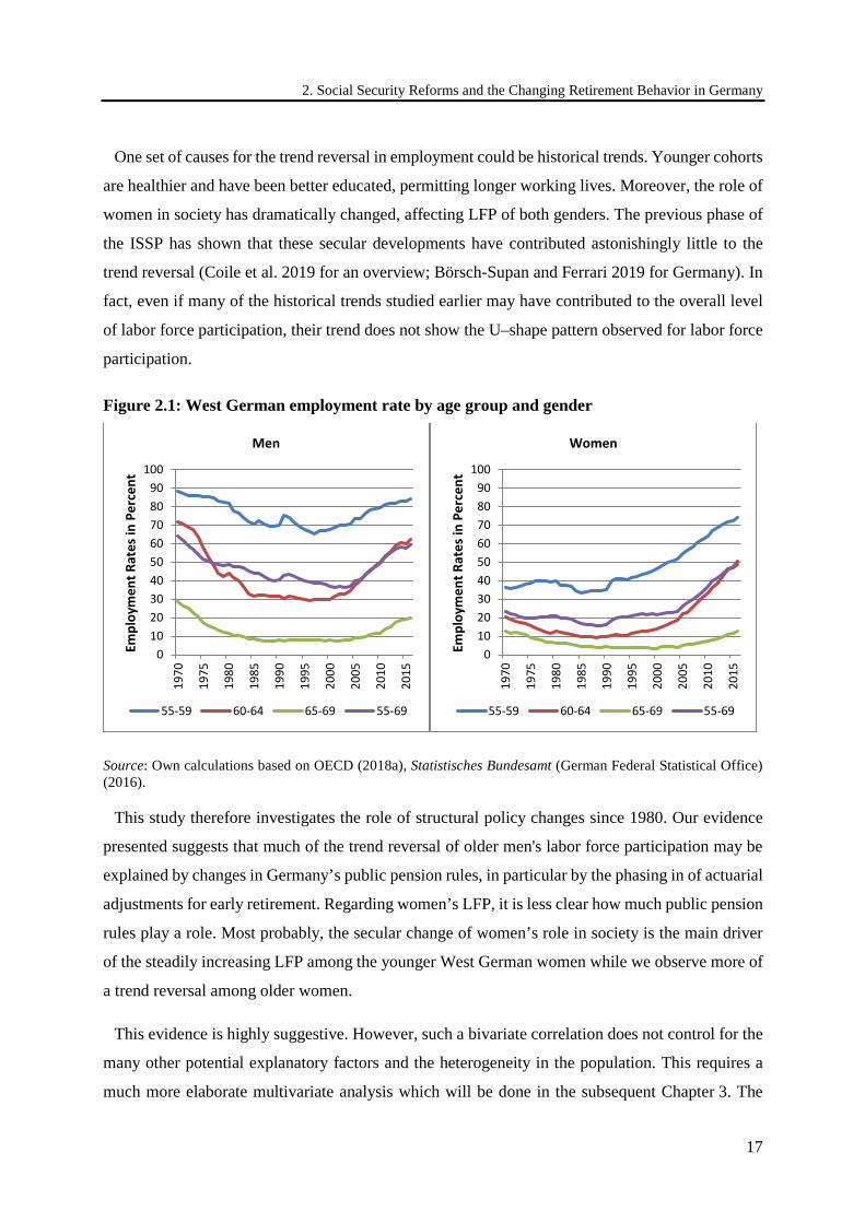
2. Social Security Reforms and the Changing Retirement Behavior in Germany
17
One set of causes for the trend reversal in employment could be historical trends. Younger cohorts
are healthier and have been better educated, permitting longer working lives. Moreover, the role of
women in society has dramatically changed, affecting LFP of both genders. The previous phase of
the ISSP has shown that these secular developments have contributed astonishingly little to the
trend reversal (Coile et al. 2019 for an overview; Börsch-Supan and Ferrari 2019 for Germany). In
fact, even if many of the historical trends studied earlier may have contributed to the overall level
of labor force participation, their trend does not show the U–shape pattern observed for labor force
participation.
Figure 2.1: West German employment rate by age group and gender
Source: Own calculations based on OECD (2018a), Statistisches Bundesamt (German Federal Statistical Office) (2016).
This study therefore investigates the role of structural policy changes since 1980. Our evidence
presented suggests that much of the trend reversal of older men's labor force participation may be
explained by changes in Germany’s public pension rules, in particular by the phasing in of actuarial
adjustments for early retirement. Regarding women’s LFP, it is less clear how much public pension
rules play a role. Most probably, the secular change of women’s role in society is the main driver
of the steadily increasing LFP among the younger West German women while we observe more of
a trend reversal among older women.
This evidence is highly suggestive. However, such a bivariate correlation does not control for the
many other potential explanatory factors and the heterogeneity in the population. This requires a
much more elaborate multivariate analysis which will be done in the subsequent Chapter 3. The
0102030405060708090
100
1970
1975
1980
1985
1990
1995
2000
2005
2010
2015
Empl
oym
ent R
ates
in P
erce
nt
Men
55-59 60-64 65-69 55-69
0102030405060708090
100
1970
1975
1980
1985
1990
1995
2000
2005
2010
2015
Empl
oym
ent R
ates
in P
erce
ntWomen
55-59 60-64 65-69 55-69
2.1 Introduction
18
analysis in Chapter 3 comprises a causal analysis of the role of public pension policies in shaping
LFP. Chapter 2 is contributing to this effort by constructing time series of the implicit tax for a
small set of stylized household types. The next step will then be to apply this machinery to real
households in a population-representative survey, and to embed our incentive variables, the macro
variables considered in Börsch-Supan and Coile (2019) and other determinants into an econometric
analysis of retirement and labor force participation.
Overall, Chapter 2 and Chapter 3 taken together contribute to the large empirical literature
studying individual retirement responses to varying incentives in the old-age security system. Both
studies are closely related to the work that was done by Gruber and Wise (1999, 2004), who
investigated the effect of retirement incentives on the downturn of labor force participation of older
individuals at the end of last century. They found that retirement incentives had a strong effect on
retirement decisions. More recent empirical investigations have shown that specific reform devices
have led to substantial reactions of older individuals’ labor market behavior, albeit at varying
magnitudes. Existing studies evaluated specific reforms such as the introduction of actuarial
adjustments for early retirement (Hanel 2010, Engels et al. 2017, Giesecke 2018), the increase of
the earliest eligibility age for early retirement (Geyer and Welteke 2017 and Geyer et al. 2020), the
reform that increased the generosity of a specific early retirement pathway for individuals with at
least 45 insurance years (Dolls and Krolage 2019), an earlier reform on supplemental pension
benefits (Ye 2018), a reform on disability insurance (Hanel 2012), and whether the 2006
unemployment insurance reform affected older workers’ labor market transitions (Riphahn and
Schrader 2019). The key novelty of Chapter 2 and Chapter 3 lies in investigating the effect of
structural policy changes on retirement and employment choices at older ages over almost four
decades. Within this period, Germany experienced a considerable reversal of employment rates and
several reforms.
Chapter 2 of this dissertation is organized as follows. Section 2.2 describes the changes in the
German labor force participation and pension claiming behavior between 1980 and 2016.
Section 2.3 provides a summary of the institutional changes and pension reforms in Germany that
may be the causes for the stunning trend reversal. Section 2.4 is the main methodological part of
the chapter and describes how we boil down the institutional changes into a few key statistics,
especially the “implicit tax on working longer”. Section 2.5 presents our results. We show how the
implicit tax on working longer has changed between 1980 and 2016, using several alternative
specifications and robustness checks. We then graphically relate the implicit tax on working longer
to the prevailing employment rate. Section 2.6 concludes. We find a negative correlation between
2. Social Security Reforms and the Changing Retirement Behavior in Germany
19
the employment rate and the incentives to claim benefits early. In other words, as the implicit tax
on working longer decreased, employment at older ages increased.
2.2 Employment rate among older individuals and pension claiming behavior
In this section, we will take a closer look at the development of the employment rate of older
workers and their actual pension claiming behavior. It is important to note that labor market exit
and the beginning of pension benefit claiming may not take place at the same time. We therefore
avoid the term “retirement” as much as we can since in many languages it ambiguously refers to
both decisions which may be driven by different considerations and determinants. We also take care
to distinguish between the group of older workers and the group of insured individuals. They do not
precisely overlap. For instance, homemakers and emigrated workers do not belong to the German
labor force but often have earned pension claims in Germany. We therefore first look at changes in
employment and later at changes in claiming behavior.
Employment rate. West Germany shares with other industrialized countries a “U-shape” pattern
in the employment rate (labor force participation rate) of older workers over time. In its downward-
phase from 1970 into the 1990s5 the employment rate of older men (age group 55-69) declined by
23.7 percentage points (pps) to 40.5% until 1990 (see Figure 2.1). Even more pronounced was this
decline for the age group 60 to 64 with a decrease by 40 pps to 31.8% until 1990. The decline was
much smaller for women with 7.1 (10.6) pps for the age group 55 to 69 (60 to 64). However, their
employment rate was with 23.5% already rather small in 1970.
5 The employment rate of whole Germany includes another drop in 1991. However, this drop results mainly from the unification of Germany and the small employment rates in East Germany. For younger age groups we also observe an increase in the employment rate after 1990 due to the unification.
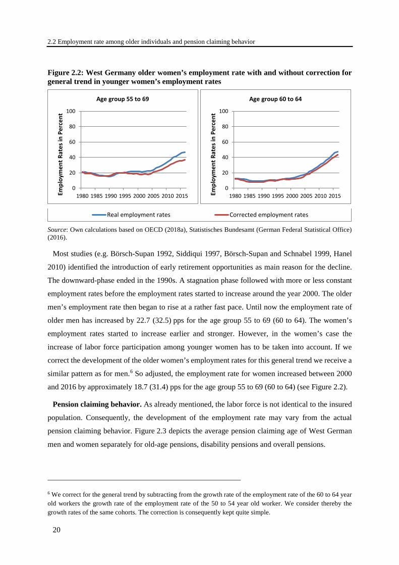
2.2 Employment rate among older individuals and pension claiming behavior
20
Figure 2.2: West Germany older women’s employment rate with and without correction for general trend in younger women’s employment rates
Source: Own calculations based on OECD (2018a), Statistisches Bundesamt (German Federal Statistical Office) (2016).
Most studies (e.g. Börsch-Supan 1992, Siddiqui 1997, Börsch-Supan and Schnabel 1999, Hanel
2010) identified the introduction of early retirement opportunities as main reason for the decline.
The downward-phase ended in the 1990s. A stagnation phase followed with more or less constant
employment rates before the employment rates started to increase around the year 2000. The older
men’s employment rate then began to rise at a rather fast pace. Until now the employment rate of
older men has increased by 22.7 (32.5) pps for the age group 55 to 69 (60 to 64). The women’s
employment rates started to increase earlier and stronger. However, in the women’s case the
increase of labor force participation among younger women has to be taken into account. If we
correct the development of the older women’s employment rates for this general trend we receive a
similar pattern as for men.6 So adjusted, the employment rate for women increased between 2000
and 2016 by approximately 18.7 (31.4) pps for the age group 55 to 69 (60 to 64) (see Figure 2.2).
Pension claiming behavior. As already mentioned, the labor force is not identical to the insured
population. Consequently, the development of the employment rate may vary from the actual
pension claiming behavior. Figure 2.3 depicts the average pension claiming age of West German
men and women separately for old-age pensions, disability pensions and overall pensions.
6 We correct for the general trend by subtracting from the growth rate of the employment rate of the 60 to 64 year old workers the growth rate of the employment rate of the 50 to 54 year old worker. We consider thereby the growth rates of the same cohorts. The correction is consequently kept quite simple.
0
20
40
60
80
100
1980 1985 1990 1995 2000 2005 2010 2015Empl
oym
ent R
ates
in P
erce
nt
Age group 55 to 69
0
20
40
60
80
100
1980 1985 1990 1995 2000 2005 2010 2015Empl
oym
ent R
ates
in P
erce
nt
Age group 60 to 64
Real employment rates Corrected employment rates
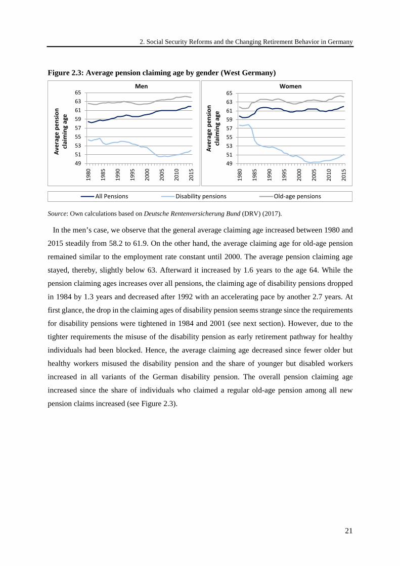
2. Social Security Reforms and the Changing Retirement Behavior in Germany
21
Figure 2.3: Average pension claiming age by gender (West Germany)
Source: Own calculations based on Deutsche Rentenversicherung Bund (DRV) (2017).
In the men’s case, we observe that the general average claiming age increased between 1980 and
2015 steadily from 58.2 to 61.9. On the other hand, the average claiming age for old-age pension
remained similar to the employment rate constant until 2000. The average pension claiming age
stayed, thereby, slightly below 63. Afterward it increased by 1.6 years to the age 64. While the
pension claiming ages increases over all pensions, the claiming age of disability pensions dropped
in 1984 by 1.3 years and decreased after 1992 with an accelerating pace by another 2.7 years. At
first glance, the drop in the claiming ages of disability pension seems strange since the requirements
for disability pensions were tightened in 1984 and 2001 (see next section). However, due to the
tighter requirements the misuse of the disability pension as early retirement pathway for healthy
individuals had been blocked. Hence, the average claiming age decreased since fewer older but
healthy workers misused the disability pension and the share of younger but disabled workers
increased in all variants of the German disability pension. The overall pension claiming age
increased since the share of individuals who claimed a regular old-age pension among all new
pension claims increased (see Figure 2.3).
495153555759616365
1980
1985
1990
1995
2000
2005
2010
2015
Aver
age
pens
ion
clai
min
g ag
e
Men
495153555759616365
1980
1985
1990
1995
2000
2005
2010
2015
Aver
age
pens
ion
clai
min
g ag
e
Women
All Pensions Disability pensions Old-age pensions
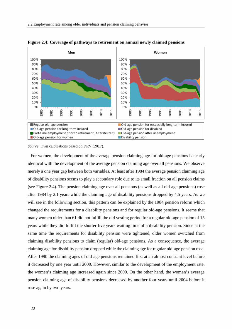
2.2 Employment rate among older individuals and pension claiming behavior
22
Figure 2.4: Coverage of pathways to retirement on annual newly claimed pensions
Source: Own calculations based on DRV (2017).
For women, the development of the average pension claiming age for old-age pensions is nearly
identical with the development of the average pension claiming age over all pensions. We observe
merely a one year gap between both variables. At least after 1984 the average pension claiming age
of disability pensions seems to play a secondary role due to its small fraction on all pension claims
(see Figure 2.4). The pension claiming age over all pensions (as well as all old-age pensions) rose
after 1984 by 2.1 years while the claiming age of disability pensions dropped by 4.5 years. As we
will see in the following section, this pattern can be explained by the 1984 pension reform which
changed the requirements for a disability pensions and for regular old-age pensions. It seems that
many women older than 61 did not fulfill the old vesting period for a regular old-age pension of 15
years while they did fulfill the shorter five years waiting time of a disability pension. Since at the
same time the requirements for disability pension were tightened, older women switched from
claiming disability pensions to claim (regular) old-age pensions. As a consequence, the average
claiming age for disability pension dropped while the claiming age for regular old-age pension rose.
After 1990 the claiming ages of old-age pensions remained first at an almost constant level before
it decreased by one year until 2000. However, similar to the development of the employment rate,
the women’s claiming age increased again since 2000. On the other hand, the women’s average
pension claiming age of disability pensions decreased by another four years until 2004 before it
rose again by two years.
0%10%20%30%40%50%60%70%80%90%
100%
1980
1985
1990
1995
2000
2005
2010
2015
Men
0%10%20%30%40%50%60%70%80%90%
100%
1980
1985
1990
1995
2000
2005
2010
2015
Women
Regular old-age pension Old-age pension for esspecially long-term insuredOld-age pension for long-term insured Old-age pension for disabledPart-time employment prior to retirement (Altersteilzeit) Old-age pension after unemploymentOld-age pension for women Disability pension
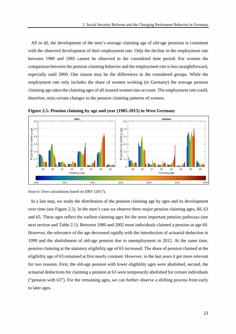
2. Social Security Reforms and the Changing Retirement Behavior in Germany
23
All in all, the development of the men’s average claiming age of old-age pensions is consistent
with the observed development of their employment rate. Only the decline in the employment rate
between 1980 and 1985 cannot be observed in the considered time period. For women the
comparison between the pension claiming behavior and the employment rate is less straightforward,
especially until 2000. One reason may be the differences in the considered groups. While the
employment rate only includes the share of women working (in Germany) the average pension
claiming age takes the claiming ages of all insured women into account. The employment rate could,
therefore, miss certain changes in the pension claiming patterns of women.
Figure 2.5: Pension claiming by age and year (1985-2015) in West Germany
Source: Own calculations based on DRV (2017).
In a last step, we study the distribution of the pension claiming age by ages and its development
over time (see Figure 2.5). In the men’s case we observe three major pension claiming ages, 60, 63
and 65. These ages reflect the earliest claiming ages for the most important pension pathways (see
next section and Table 2.1). Between 1980 and 2002 most individuals claimed a pension at age 60.
However, the relevance of the age decreased rapidly with the introduction of actuarial deduction in
1999 and the abolishment of old-age pension due to unemployment in 2012. At the same time,
pension claiming at the statutory eligibility age of 65 increased. The share of pension claimed at the
eligibility age of 63 remained at first nearly constant. However, in the last years it got more relevant
for two reasons. First, the old-age pension with lower eligibility ages were abolished, second, the
actuarial deductions for claiming a pension at 63 were temporarily abolished for certain individuals
(“pension with 63”). For the remaining ages, we can further observe a shifting process from early
to later ages.

2.2 Employment rate among older individuals and pension claiming behavior
24
For women two major pension claiming ages can be observed. First, the eligibility age for the old-
age pension for women at age 60 and second the statutory eligibility age at 65. Similar to the men’s
case the share of pension claiming at age 60 declined after 1999 in two steps. The first drop after
1999 reduced the share on all pension claiming by almost 20 pps while the second drop, which
occurred 2012 (abolishment of the old-age pension for women), covered a decline of 15 pps. At the
same time the earliest eligibility age for long-term insured (age 63) became more relevant. In total,
the share of women claiming a pension at age 63 increased from 2.4% to 28.2%. Nonetheless, with
over 40 percent, most women claimed their pension at the statutory eligibility age. Similar to the
men’s case, between the ages 60 and 63, a shifting process can be observed – which moves the
pension claiming from younger to older ages.
2. Social Security Reforms and the Changing Retirement Behavior in Germany
25
2.3 Institutional changes: German pension policy and its development
The main hypothesis of this study is that the reversals in labor supply and pension claiming behavior
around the year 2000 are to a large extent driven by changes in pension policies. To this end, this
section presents the policy changes that occurred since 1980 and are salient for changes in
retirement behavior. We start with a brief summary of the structure of the German pension system
in 1980 in order to assess the initial situation of the system at the beginning of the time span
considered in this study.
2.3.1 German pension system until 1980
The German pension system originally began as a funded disability insurance scheme in 1889. In
the beginning, “old age” was classified as a subcategory of disability. “Disability benefits due to
old age” were lower compared to real disability benefits and were granted starting from age 70.
With further reforms in the following years (in particular in 1899, 1911, 1913, 1916), the scheme
was broadened into a general old-age security system with disability pensions and mere old-age
pensions. Benefits of disability pensions and old-age pensions were set on the same level and the
coverage among workers and employees was increasingly enlarged. The eligibility age was lowered
to 65, first for employees in 1913 and for workers in 1916 (DRV 2020). After two world wars and
a period of hyperinflation about half of the capital stock was lost and the system was transformed
into a pay-as-you-go (PAYG) system in 1957. Benefits from this public PAYG system were
designed to maintain the living standard that was achieved during the working life to the time of
retirement. Therefore, individual pension benefits were set to be proportional to the individual labor
income averaged over the entire working career such that the relative income position of an
individual during the working life would be preserved during retirement. While the absolute level
of pension benefits has been reduced in the subsequent reforms, the principle of maintaining the
relative income position has been preserved until today. The German public pension system
therefore features only few redistributive properties, much less than, e.g., the US Social Security
system. The main redistribution instrument to prevent old-age poverty is a kind of minimum pension
at the social assistance level that was introduced in 2001. The system is mandatory for all workers
except for most self-employed, civil servants and workers with earnings below the official
minimum earnings threshold. In the case of the main earner’s death spouses and children are
additionally protected through survivor benefits.
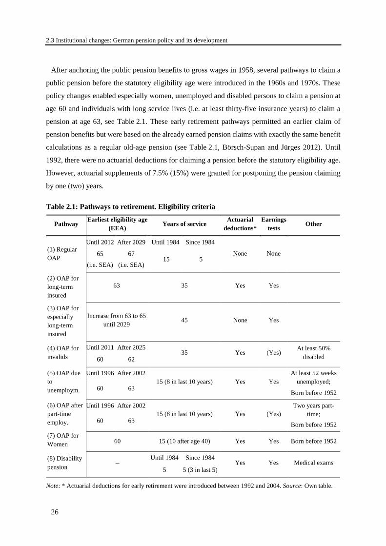
2.3 Institutional changes: German pension policy and its development
26
After anchoring the public pension benefits to gross wages in 1958, several pathways to claim a
public pension before the statutory eligibility age were introduced in the 1960s and 1970s. These
policy changes enabled especially women, unemployed and disabled persons to claim a pension at
age 60 and individuals with long service lives (i.e. at least thirty-five insurance years) to claim a
pension at age 63, see Table 2.1. These early retirement pathways permitted an earlier claim of
pension benefits but were based on the already earned pension claims with exactly the same benefit
calculations as a regular old-age pension (see Table 2.1, Börsch-Supan and Jürges 2012). Until
1992, there were no actuarial deductions for claiming a pension before the statutory eligibility age.
However, actuarial supplements of 7.5% (15%) were granted for postponing the pension claiming
by one (two) years.
Table 2.1: Pathways to retirement. Eligibility criteria
Pathway Earliest eligibility age
(EEA) Years of service
Actuarial deductions*
Earnings tests
Other
(1) Regular OAP
Until 2012 After 2029 Until 1984 Since 1984
None None
65
(i.e. SEA)
67
(i.e. SEA) 15 5
(2) OAP for long-term insured
63 35 Yes Yes
(3) OAP for especially long-term insured
Increase from 63 to 65 until 2029
45 None Yes
(4) OAP for invalids
Until 2011 After 2025 35 Yes (Yes)
At least 50% disabled 60 62
(5) OAP due to unemploym.
Until 1996 After 2002 15 (8 in last 10 years) Yes Yes
At least 52 weeks unemployed;
Born before 1952 60 63
(6) OAP after part-time employ.
Until 1996 After 2002 15 (8 in last 10 years) Yes (Yes)
Two years part-time;
Born before 1952 60 63
(7) OAP for Women 60 15 (10 after age 40) Yes Yes Born before 1952
(8) Disability pension –
Until 1984 Since 1984 Yes Yes Medical exams
5 5 (3 in last 5)
Note: * Actuarial deductions for early retirement were introduced between 1992 and 2004. Source: Own table.
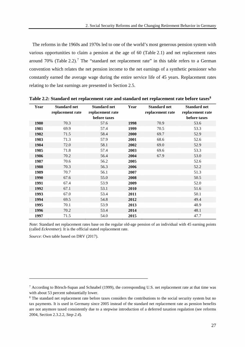
2. Social Security Reforms and the Changing Retirement Behavior in Germany
27
The reforms in the 1960s and 1970s led to one of the world’s most generous pension system with
various opportunities to claim a pension at the age of 60 (Table 2.1) and net replacement rates
around 70% (Table 2.2).7 The “standard net replacement rate” in this table refers to a German
convention which relates the net pension income to the net earnings of a synthetic pensioner who
constantly earned the average wage during the entire service life of 45 years. Replacement rates
relating to the last earnings are presented in Section 2.5.
Table 2.2: Standard net replacement rate and standard net replacement rate before taxes8
Year Standard net replacement rate
Standard net replacement rate
before taxes
Year Standard net replacement rate
Standard net replacement rate
before taxes 1980 70.3 57.6 1998 70.9 53.6 1981 69.9 57.4 1999 70.5 53.3 1982 71.5 58.4 2000 69.7 52.9 1983 71.3 57.9 2001 68.6 52.6 1984 72.0 58.1 2002 69.0 52.9 1985 71.8 57.4 2003 69.6 53.3 1986 70.2 56.4 2004 67.9 53.0 1987 70.6 56.2 2005 52.6 1988 70.3 56.3 2006 52.2 1989 70.7 56.1 2007 51.3 1990 67.6 55.0 2008 50.5 1991 67.4 53.9 2009 52.0 1992 67.1 53.1 2010 51.6 1993 67.0 53.4 2011 50.1 1994 69.5 54.8 2012 49.4 1995 70.1 53.9 2013 48.9 1996 70.2 53.4 2014 48.1 1997 71.5 54.0 2015 47.7
Note: Standard net replacement rates base on the regular old-age pension of an individual with 45 earning points (called Eckrentner). It is the official stated replacement rate.
Source: Own table based on DRV (2017).
7 According to Börsch-Supan and Schnabel (1999), the corresponding U.S. net replacement rate at that time was with about 53 percent substantially lower. 8 The standard net replacement rate before taxes considers the contributions to the social security system but no tax payments. It is used in Germany since 2005 instead of the standard net replacement rate as pension benefits are not anymore taxed consistently due to a stepwise introduction of a deferred taxation regulation (see reforms 2004, Section 2.3.2.2, Step 2.4).
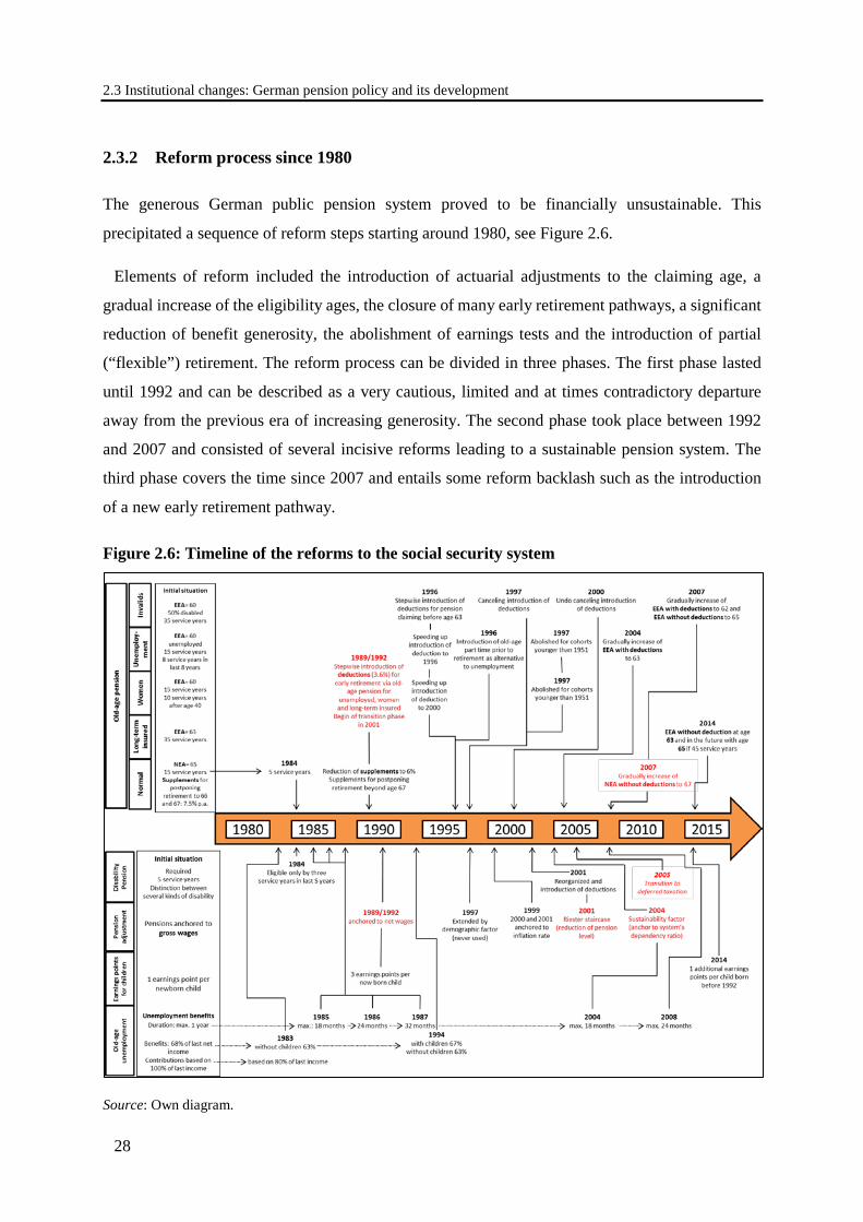
2.3 Institutional changes: German pension policy and its development
28
2.3.2 Reform process since 1980
The generous German public pension system proved to be financially unsustainable. This
precipitated a sequence of reform steps starting around 1980, see Figure 2.6.
Elements of reform included the introduction of actuarial adjustments to the claiming age, a
gradual increase of the eligibility ages, the closure of many early retirement pathways, a significant
reduction of benefit generosity, the abolishment of earnings tests and the introduction of partial
(“flexible”) retirement. The reform process can be divided in three phases. The first phase lasted
until 1992 and can be described as a very cautious, limited and at times contradictory departure
away from the previous era of increasing generosity. The second phase took place between 1992
and 2007 and consisted of several incisive reforms leading to a sustainable pension system. The
third phase covers the time since 2007 and entails some reform backlash such as the introduction
of a new early retirement pathway.
Figure 2.6: Timeline of the reforms to the social security system
Source: Own diagram.
2. Social Security Reforms and the Changing Retirement Behavior in Germany
29
2.3.2.1 Phase 1 (1980 to 1992): modest retrenchment within the pension system/increasing
generosity outside the pension system
In the 1984 reform, the requirements for disability pensions were tightened by making a minimum
of three contribution years in the last five years a necessary condition. Moreover, stricter medical
examinations were introduced. As kind of compensation, the vesting period for regular old-age
pensions was reduced from 15 to five service years. Together this gravely changed the balance
between newly claimed old-age pension and disability pension in favor of old-age pensions. As
Figure 2.4 depicts, this was especially the case for the women’s pension claiming behavior. The
share of claimed disability pensions on all newly claimed pension dropped for women by over
30 pps while the share of regular old-age pension increased by the same amount. This strong effect
has two reasons. First, the number of women fulfilling the new requirements for disability pensions
dropped, as many women stopped working after marriage or childbirth and had therefore paid no
contributions in the last five years. Second, due to similar reasons, women may have only been able
to claim disability pensions as they did not fulfilled the former vesting period of 15 service years
for a regular old-age pension.
In a contradictory move, the opportunity to leave the labor market early was widened between
1984 and 1987 by extending the maximal duration time of unemployment benefits for older workers
(age 56 and above) from 12 months to 32 months. In fact, since unemployment benefits are neither
means-tested nor do they require job search attempts they are often used “to build a bridge to
retirement”. The extension of the duration time widened this “bridge”. Moreover, severance pay
became tax advantageous for employers. This further facilitated a mutual agreement among
employers and employees regarding ending the employment relationship with the right to claim
unemployment benefits.
2.3.2.2 Phase 2 (1992 to 2007): sustainability reforms
Step 2.1 (1992): Toward actuarial adjustments and more flexibility
The 1992 pension reform, which passed the parliament in 1989, represents a significant landmark
in the German pension policy as it marks the leap into an era of reforms striving to increase the
system’s sustainability. As a first step of this process, the 1992 pension reform introduced two
significant changes to the pension system’s framework. First, it switched the benefit adjustment
from gross wage growth to net wage growth. This measure got rid of an odd situation where
increasing social contribution rates would have led to a circle of rising net replacement rates.
2.3 Institutional changes: German pension policy and its development
30
Second, starting in 2001 it provided a phased introduction (by cohorts) of actuarial adjustments for
an early pension claiming. This measure started a long sequence of changes in the system of
pathways to retirement and their eligibility ages with and without actuarial adjustments. They are
graphically displayed in Figure 2.7 at the end of this section; each panel a) through h) presents an
element in this sequence.
The stepwise introduction of actuarial adjustments dealt with the strong incentives to claim a
pension early as they reduce pension benefits by 3.6% per year of early pension claiming (counted
from the statutory eligibility age or a respective earlier adjustment-free eligibility age, see
Table 2.6). However, these actuarial adjustments are not actuarial neutral as several studies showed
(see Werding 2007, 2012 and Gasche 2012); hence an incentive to claim a pension early remains.
Proper actuarial neutral adjustment would have to be at least twice as large as the current ones.
Parallel to the introduction of actuarial deduction, the actuarial supplements for postponing the
pension claiming beyond the statutory eligibility age were changed. From 1992 onward actuarial
supplements were granted for each year of later pension claiming (not only for the first two years).
However, at the same time the actuarial supplements were reduced to six percent per year of later
retirement (actuarial deduction of 20%).
Beside these sustainability-increasing measures, the 1992 pension reform contained two
additional components. First, the number of earnings points parents receive for newborn children
were increased from one to three. Second, a partial old-age pension was introduced which enabled
individuals to compensate an income loss due to a reduction in working hours (part-time work) by
drawing a partial pension. The partial pension could be drawn, however, only for certain proportions
of the split between work and retirement: one third, one half, or two thirds. The earning limits were
calculated individually based on the labor income of the last three years before drawing the partial
pension. In the end, this pension scheme was not overly successful as very few individuals used it.
In 1996, the timetable for the introduction of the actuarial adjustment was moved up to 1997 for
the old-age pension due to unemployment and to 2000 for the old-age pension for women (see
Figure 2.7c). Moreover, it was decided to phase in actuarial adjustments for the old-age pension for
disabled persons (see Table 2.6).
2. Social Security Reforms and the Changing Retirement Behavior in Germany
31
Parallel, the old-age pension due to unemployment was expanded to also include part-time
workers prior retirement for employees over 55 (Altersteilzeit).9 This represented the so far most
widely used model of pre-retirement work reduction. The scheme is based on a bilateral agreement
between employee and employer and required a reduction of working hours by half in the last five
years before the public pension is claimed. The remaining “half” working time could be distributed
either consistent over the whole period of five years or could be fulfilled entirely in the first two
and a half years without a reduction in working, the “block model”. In both cases, the employee
receives an ongoing payment composed of their part-time work income and a supplementary
income of 20% by the employer. Additionally, the employer pays pension contributions for 80% of
the part-time work income. The scheme is subsidized in the sense that the supplementary
compensation by the employer is tax exempted (see Börsch-Supan et al. 2015).
Step 2.2 (1997): Closing early retirement schemes and the demographic factor
In December 1997 a reform package passed the German parliament which (would have) included
three crucial components to further increase the sustainability of the Germen pension system. First,
the old-age pension due to unemployment and for women were abolished for cohorts born after
1952 (see Figure 2.7d); second, the pension adjustment indexation formula was amended by a
demographic factor which would have adapted the benefit growth to the demographic development;
and third, actuarial adjustments were introduced for disability pensions. Other than for the old-age
pensions the actuarial adjustments were, however, limited to 10.8% and depended on the distance
between the claiming of a disability pension and the age 63. Moreover, the pre-adjusted disability
pension benefits were enlarged if the act of disability happened before the age of 60, which
compensated for a major part of the newly introduced actuarial adjustments. The reform package
itself should have become effective in 1999. However, the 1998 new elected government of Social
Democrats and Green Party suspended the second and third component of the reform package
(demographic factor and changes to the disability pension) in order to find a more social regulation.
For 2000 and 2001, the benefit adjustment was aligned to the inflation rate.
Step 2.3 (2000 till 2001): Toward a genuine multipillar system
The new government presented the revised pension plan in 2000 and 2001. Regarding the disability
pension, the new government adopted the plans of the former government, meaning the introduction
9 For readability reasons we will continue to call this pension scheme old-age pension due to unemployment.
2.3 Institutional changes: German pension policy and its development
32
of actuarial adjustments combined with an improvement of the disability benefits (see Table 2.6
and Figure 2.7e). The previous version of the disability pension covered vocational disability
(Berufsunfähigkeit, BU) and “real” disability (Erwerbsunfähigkeit, EU). This distinction was
abolished in favor for a two-step disability pension (partial/full earning incapacity) with strict health
tests. Whether a disabled individual is eligible for a partial or full disability pension depends on his
maximal working capacity (less than six hours per day for a partial disability pension or less than
three hours per day for a full rate disability pension). The new disability pension became effective
in 2001.
In the same year, the Riester reforms took place which entailed a major reorganization of the
German pension system by converting the formally monolithic pay-as-you-go pension scheme into
a genuine multi-pillar system. With this reform, the pay-as-you-go financed system was partial
substituted by a (not mandatory) subsidized private funded system (Riester-Rente). The benefits of
the original system were therefore gradually reduced in proportion to the maximal subsidized
contribution rate of the newly created supplementary pension scheme (see decreasing replacement
rates in Table 2.2). This was done by adding an appropriate component into the pension benefit
indexation formula.10 The side effect of this rearrangement was that the pay-as-you-go system was
relieved. This corresponded with the second aim of the Riester reform to stabilize the contribution
rate by reducing the pension level. Actually, the Riester reform law stated that the contribution rate
to the public retirement insurance must stay below 20% until 2020 and below 22% until 2030, while
the standard net replacement rate must stay above 67%. Failure must precipitate further government
actions.
Step 2.4 (2004): Toward Sustainability (sustainability factor)
It quickly became obvious that the contribution rate thresholds could not be fulfilled without further
cost-cutting measures. As a consequence, the Commission for Sustainability in Financing the
German Social Insurance Systems was established to develop appropriate reform plans at the end
of 2002. In the following year, the commission proposed an entire reform package (Commission
2003) with two key components. First, the commission encouraged the government to anchor the
10 The new component represented solely the growth rate of the pension system’s contribution rate. This component replaced the former one introduced with the 1989 reform that had linked benefits to net wage growth. Due to this novelty, changes in the balance between the fiscal burden of pensions and wages had no longer an influence on the adjustment of the pensions.
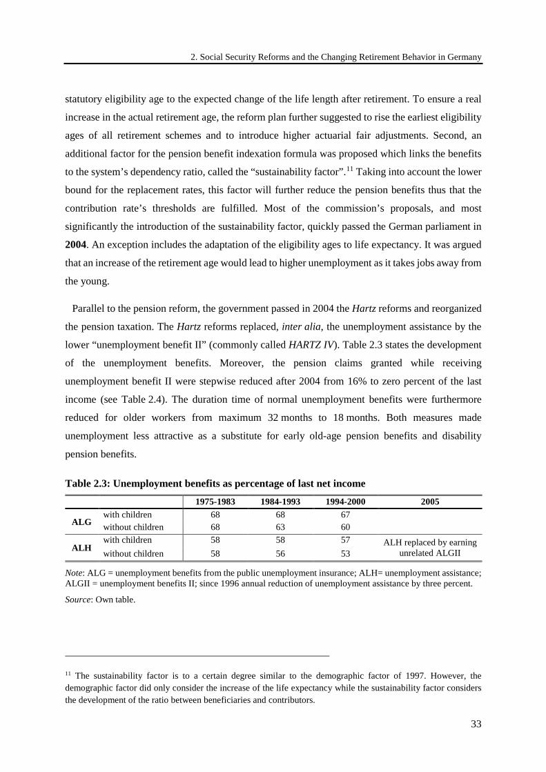
2. Social Security Reforms and the Changing Retirement Behavior in Germany
33
statutory eligibility age to the expected change of the life length after retirement. To ensure a real
increase in the actual retirement age, the reform plan further suggested to rise the earliest eligibility
ages of all retirement schemes and to introduce higher actuarial fair adjustments. Second, an
additional factor for the pension benefit indexation formula was proposed which links the benefits
to the system’s dependency ratio, called the “sustainability factor”.11 Taking into account the lower
bound for the replacement rates, this factor will further reduce the pension benefits thus that the
contribution rate’s thresholds are fulfilled. Most of the commission’s proposals, and most
significantly the introduction of the sustainability factor, quickly passed the German parliament in
2004. An exception includes the adaptation of the eligibility ages to life expectancy. It was argued
that an increase of the retirement age would lead to higher unemployment as it takes jobs away from
the young.
Parallel to the pension reform, the government passed in 2004 the Hartz reforms and reorganized
the pension taxation. The Hartz reforms replaced, inter alia, the unemployment assistance by the
lower “unemployment benefit II” (commonly called HARTZ IV). Table 2.3 states the development
of the unemployment benefits. Moreover, the pension claims granted while receiving
unemployment benefit II were stepwise reduced after 2004 from 16% to zero percent of the last
income (see Table 2.4). The duration time of normal unemployment benefits were furthermore
reduced for older workers from maximum 32 months to 18 months. Both measures made
unemployment less attractive as a substitute for early old-age pension benefits and disability
pension benefits.
Table 2.3: Unemployment benefits as percentage of last net income
1975-1983 1984-1993 1994-2000 2005
ALG with children 68 68 67 without children 68 63 60
ALH with children 58 58 57 ALH replaced by earning
unrelated ALGII without children 58 56 53
Note: ALG = unemployment benefits from the public unemployment insurance; ALH= unemployment assistance; ALGII = unemployment benefits II; since 1996 annual reduction of unemployment assistance by three percent.
Source: Own table.
11 The sustainability factor is to a certain degree similar to the demographic factor of 1997. However, the demographic factor did only consider the increase of the life expectancy while the sustainability factor considers the development of the ratio between beneficiaries and contributors.

2.3 Institutional changes: German pension policy and its development
34
Table 2.4: Contribution to public pension system for unemployed as percentage of last gross income
until 1978 1979-1982 1983-1999 2000-2004 2005-2006 2007-2010 since 2011
ALG 80 100 80 80 80 80 80 ALH/ALGII 80 100 80 ca. 32 ca. 16 ca. 8 none
Note: ALG = unemployment benefits from the public unemployment insurance; ALH = unemployment assistance replaced by the unemployment benefits II (ALG II) in 2005; paid contributions indicates collected pension claims (earnings points) while unemployed.
Source: Own table.
2. Social Security Reforms and the Changing Retirement Behavior in Germany
35
Due to a decision by the Federal Constitutional Court, which was prompted by differential taxation
of public pension benefits and the pensions of civil servants, the pension taxation system was
reorganized (see Börsch-Supan and Quinn 2015). Until 2004 public pensions were only taxed if
they surpassed a quite large allowance. Actually, this only applied to relative few cases. With the
new regulations, a deferred taxation of pension was introduced. Hence, the contributions to the
pension insurance became tax exempt and the pension benefits taxable. To prevent a double taxation
the reform included a generous transition period.12
Step 2.5 (2007): Toward later retirement ages
In the end, population aging remained high on the political agenda and so the yet not implemented
reform proposal of the commission, namely the increase of eligibility ages. Finally in 2007 the then
Federal Minister of Labor and Social Affairs Franz Müntefering surprisingly unilaterally announced
the increase of the statutory eligibility age similar to the suggestion of the commission until 2029
(see Figure 2.7g black and blue line).13 Parallel, the benchmarks for adjustment free disability
pensions should be raised from 63 to 65. In contrast, the adoption of the earliest eligibility scheme
(old-age pension for workers with a long service history) to life expectancy (see Figure 2.7g blue
dotted line) as well as the introduction of actuarial fair adjustments (see Table 2.6 for cohort-
specific actuarial adjustments) remained unrealized.
2.3.2.3 Phase 3 (2007 to 2016): reform backlash, the “pension with 63”
In the 2007 pension reform the process toward a sustainable pension system ended and a phase of
moderate reform backlashes followed. This process actually already began within the 2007 pension
reform as the decision to increase the statutory eligibility age was weakened by exemptions for
those workers who have forty-five years with active contribution payments (see Figure 2.7g orange
line). This new type of old-age pensions (“old-age pension for especially long careers”) could be
claimed at the age 65 or older, but not earlier, even with actuarial adjustments. The next backlash
12 The transition included, on the one hand side, an implementation of the tax exemption between 2005 and 2025 and, on the other hand, a constant tax allowances on pension claimed before 2040. The tax exemption increases stepwise from 60% to 100%. For pension claimed before 2005 the tax allowance was set to 50% of the gross pension benefits in 2005. For pensions claimed between 2005 and 2040 the allowance is a fraction of the first received gross pension whereby the fraction itself depends on the pension claiming year and decreases from 50% to zero percent. 13 Note that the statutory eligibility age was not automatically linked to life expectancy.
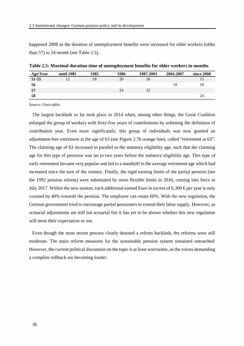
2.3 Institutional changes: German pension policy and its development
36
happened 2008 as the duration of unemployment benefits were increased for older workers (older
than 57) to 24 month (see Table 2.5).
Table 2.5: Maximal duration time of unemployment benefits for older workers in months
Age\Year until 1985 1985 1986 1987-2003 2004-2007 since 2008 51-55 12 18 20 26
15
56
18 18 57
24 32
58
24
Source: Own table.
The largest backlash so far took place in 2014 when, among other things, the Great Coalition
enlarged the group of workers with forty-five years of contributions by softening the definition of
contribution year. Even more significantly, this group of individuals was now granted an
adjustment-free retirement at the age of 63 (see Figure 2.7h orange line), called “retirement at 63”.
The claiming age of 63 increased in parallel to the statutory eligibility age, such that the claiming
age for this type of pensions was set to two years before the statutory eligibility age. This type of
early retirement became very popular and led to a standstill in the average retirement age which had
increased since the turn of the century. Finally, the rigid earning limits of the partial pension (see
the 1992 pension reform) were substituted by more flexible limits in 2016, coming into force in
July 2017. Within the new system, each additional earned Euro in excess of 6,300 € per year is only
counted by 40% towards the pension. The employee can retain 60%. With the new regulation, the
German government tried to encourage partial pensioners to extend their labor supply. However, as
actuarial adjustments are still not actuarial fair it has yet to be shown whether this new regulation
will meet their expectation or not.
Even though the most recent process clearly denoted a reform backlash, the reforms were still
moderate. The main reform measures for the sustainable pension system remained untouched.
However, the current political discussion on the topic is at least worrisome, as the voices demanding
a complete rollback are becoming louder.
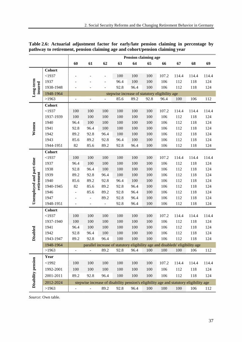
2. Social Security Reforms and the Changing Retirement Behavior in Germany
37
Table 2.6: Actuarial adjustment factor for early/late pension claiming in percentage by pathway to retirement, pension claiming age and cohort/pension claiming year
Pension claiming age
60 61 62 63 64 65 66 67 68 69 Cohort
Lon
g-te
rm
insu
red
<1937 - - - 100 100 100 107.2 114.4 114.4 114.4 1937 - - - 96.4 100 100 106 112 118 124 1938-1948 - - - 92.8 96.4 100 106 112 118 124 1948-1964 stepwise increase of statutory eligibility age >1963 - - - 85.6 89.2 92.8 96.4 100 106 112 Cohort
Wom
en
<1937 100 100 100 100 100 100 107.2 114.4 114.4 114.4 1937-1939 100 100 100 100 100 100 106 112 118 124 1940 96.4 100 100 100 100 100 106 112 118 124 1941 92.8 96.4 100 100 100 100 106 112 118 124 1942 89.2 92.8 96.4 100 100 100 106 112 118 124 1943 85.6 89.2 92.8 96.4 100 100 106 112 118 124 1944-1951 82 85.6 89.2 92.8 96.4 100 106 112 118 124 Cohort
Une
mpl
oyed
and
par
t-tim
e re
tirem
ent
<1937 100 100 100 100 100 100 107.2 114.4 114.4 114.4 1937 96.4 100 100 100 100 100 106 112 118 124 1938 92.8 96.4 100 100 100 100 106 112 118 124 1939 89.2 92.8 96.4 100 100 100 106 112 118 124 1940 85.6 89.2 92.8 96.4 100 100 106 112 118 124 1940-1945 82 85.6 89.2 92.8 96.4 100 106 112 118 124 1946 - 85.6 89.2 92.8 96.4 100 106 112 118 124 1947 - - 89.2 92.8 96.4 100 106 112 118 124 1948-1951 - - - 92.8 96.4 100 106 112 118 124
Cohort
Dis
able
d
<1937 100 100 100 100 100 100 107.2 114.4 114.4 114.4 1937-1940 100 100 100 100 100 100 106 112 118 124 1941 96.4 100 100 100 100 100 106 112 118 124 1942 92.8 96.4 100 100 100 100 106 112 118 124 1943-1947 89.2 92.8 96.4 100 100 100 106 112 118 124 1948-1964 parallel increase of statutory eligibility age and disableds' eligibility age >1963 - - 89.2 92.8 96.4 100 100 100 106 112
Dis
abili
ty p
ensi
on Year
<1992 100 100 100 100 100 100 107.2 114.4 114.4 114.4 1992-2001 100 100 100 100 100 100 106 112 118 124 2001-2011 89.2 92.8 96.4 100 100 100 106 112 118 124
2012-2024 stepwise increase of disability pension's eligibility age and statutory eligibility age >1963 - - 89.2 92.8 96.4 100 100 100 106 112
Source: Own table.
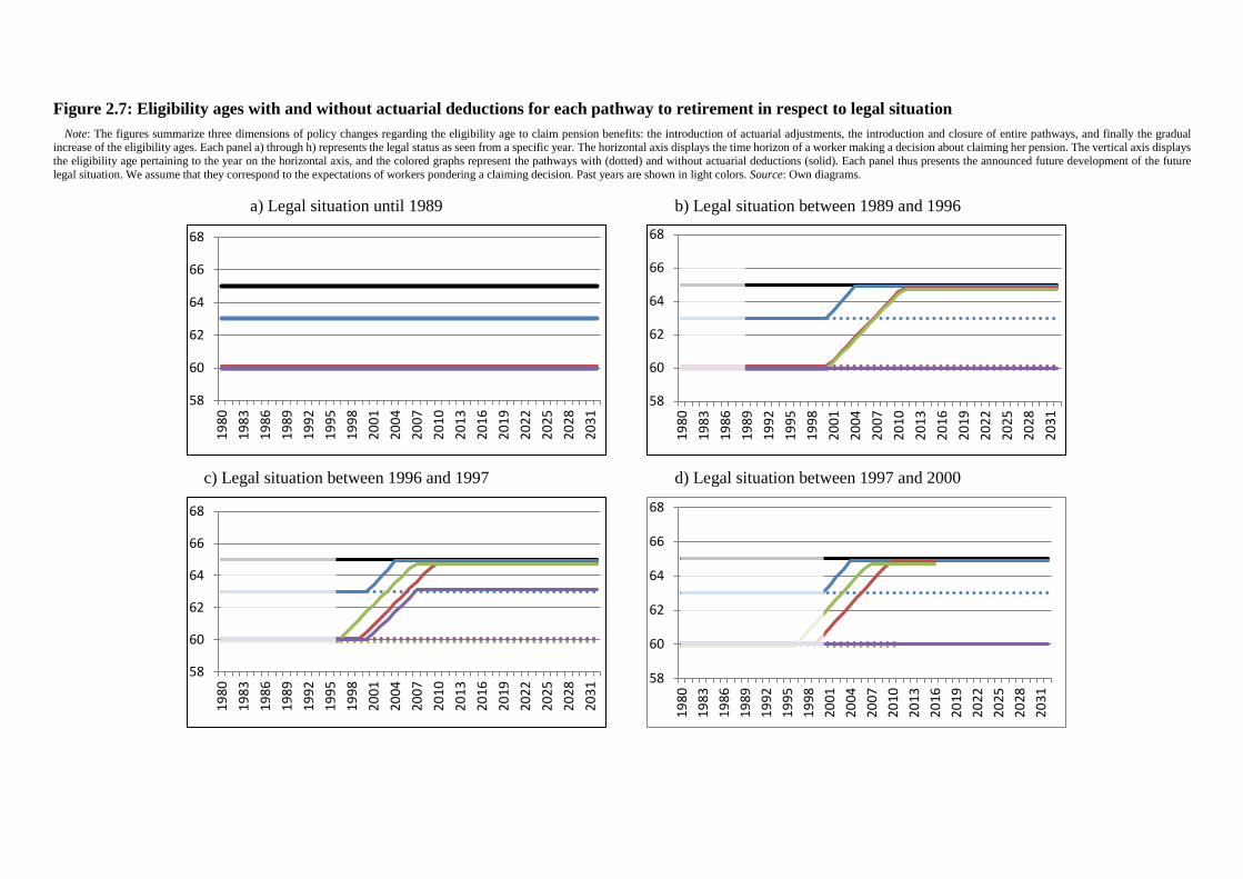
Figure 2.7: Eligibility ages with and without actuarial deductions for each pathway to retirement in respect to legal situation Note: The figures summarize three dimensions of policy changes regarding the eligibility age to claim pension benefits: the introduction of actuarial adjustments, the introduction and closure of entire pathways, and finally the gradual
increase of the eligibility ages. Each panel a) through h) represents the legal status as seen from a specific year. The horizontal axis displays the time horizon of a worker making a decision about claiming her pension. The vertical axis displays the eligibility age pertaining to the year on the horizontal axis, and the colored graphs represent the pathways with (dotted) and without actuarial deductions (solid). Each panel thus presents the announced future development of the future legal situation. We assume that they correspond to the expectations of workers pondering a claiming decision. Past years are shown in light colors. Source: Own diagrams.
a) Legal situation until 1989 b) Legal situation between 1989 and 1996
c) Legal situation between 1996 and 1997 d) Legal situation between 1997 and 2000
58
60
62
64
66
6819
8019
8319
8619
8919
9219
9519
9820
0120
0420
0720
1020
1320
1620
1920
2220
2520
2820
31
58
60
62
64
66
68
1980
1983
1986
1989
1992
1995
1998
2001
2004
2007
2010
2013
2016
2019
2022
2025
2028
2031
58
60
62
64
66
68
1980
1983
1986
1989
1992
1995
1998
2001
2004
2007
2010
2013
2016
2019
2022
2025
2028
2031
58
60
62
64
66
68
1980
1983
1986
1989
1992
1995
1998
2001
2004
2007
2010
2013
2016
2019
2022
2025
2028
2031
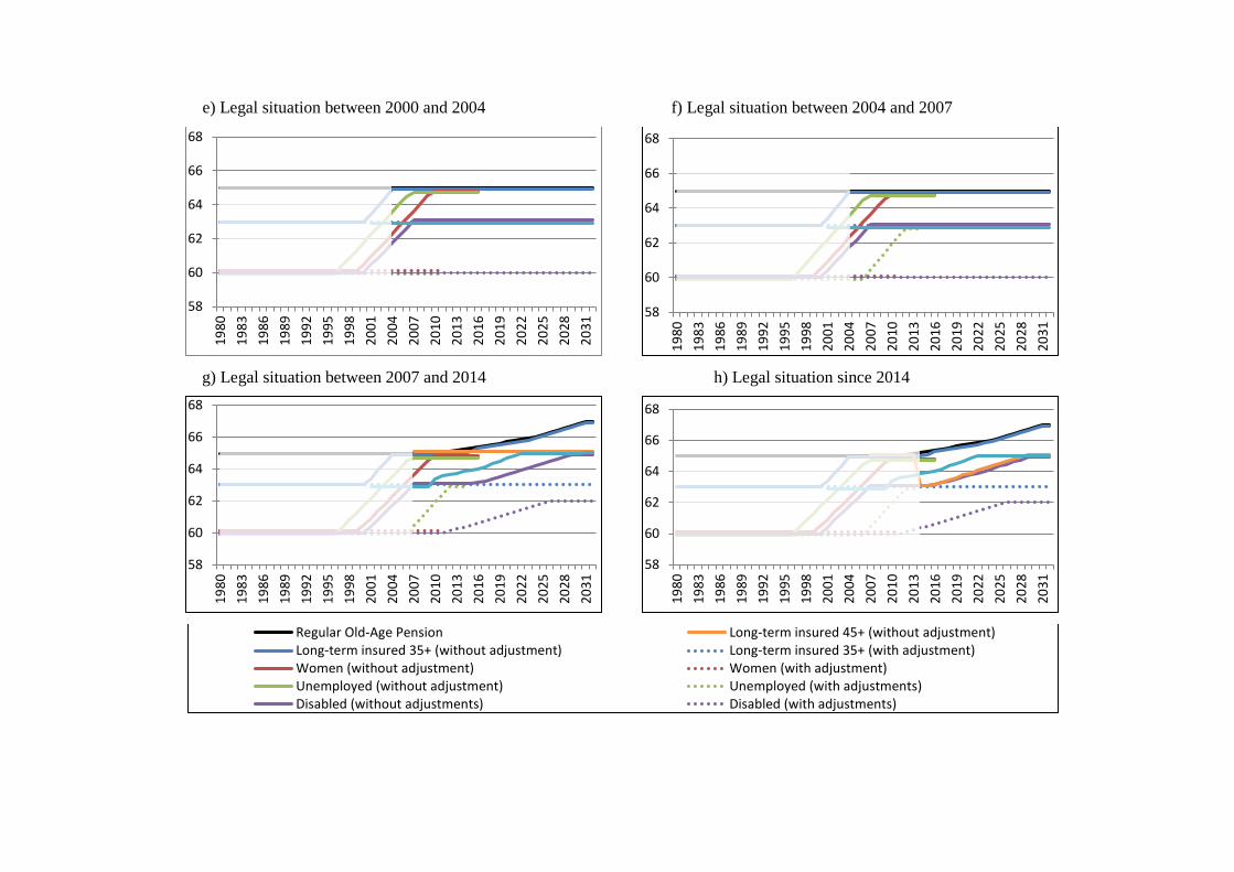
39
e) Legal situation between 2000 and 2004 f) Legal situation between 2004 and 2007
g) Legal situation between 2007 and 2014 h) Legal situation since 2014
58
60
62
64
66
68
1980
1983
1986
1989
1992
1995
1998
2001
2004
2007
2010
2013
2016
2019
2022
2025
2028
2031
58
60
62
64
66
68
1980
1983
1986
1989
1992
1995
1998
2001
2004
2007
2010
2013
2016
2019
2022
2025
2028
2031
58
60
62
64
66
68
1980
1983
1986
1989
1992
1995
1998
2001
2004
2007
2010
2013
2016
2019
2022
2025
2028
2031
58
60
62
64
66
68
1980
1983
1986
1989
1992
1995
1998
2001
2004
2007
2010
2013
2016
2019
2022
2025
2028
2031
Regular Old-Age Pension Long-term insured 45+ (without adjustment)Long-term insured 35+ (without adjustment) Long-term insured 35+ (with adjustment)Women (without adjustment) Women (with adjustment)Unemployed (without adjustment) Unemployed (with adjustments)Disabled (without adjustments) Disabled (with adjustments)
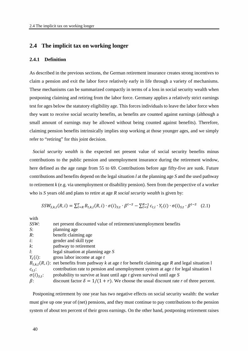
2.4 The implicit tax on working longer
40
2.4 The implicit tax on working longer
2.4.1 Definition
As described in the previous sections, the German retirement insurance creates strong incentives to
claim a pension and exit the labor force relatively early in life through a variety of mechanisms.
These mechanisms can be summarized compactly in terms of a loss in social security wealth when
postponing claiming and retiring from the labor force. Germany applies a relatively strict earnings
test for ages below the statutory eligibility age. This forces individuals to leave the labor force when
they want to receive social security benefits, as benefits are counted against earnings (although a
small amount of earnings may be allowed without being counted against benefits). Therefore,
claiming pension benefits intrinsically implies stop working at those younger ages, and we simply
refer to “retiring” for this joint decision.
Social security wealth is the expected net present value of social security benefits minus
contributions to the public pension and unemployment insurance during the retirement window,
here defined as the age range from 55 to 69. Contributions before age fifty-five are sunk. Future
contributions and benefits depend on the legal situation l at the planning age S and the used pathway
to retirement k (e.g. via unemployment or disability pension). Seen from the perspective of a worker
who is S years old and plans to retire at age R social security wealth is given by:
𝑆𝑆𝑆𝑆𝑊𝑊𝑆𝑆,𝑘𝑘,𝑙𝑙(𝑅𝑅, 𝑖𝑖) = ∑ 𝐵𝐵𝑡𝑡,𝑘𝑘,𝑙𝑙(𝑅𝑅, 𝑖𝑖) ∙ 𝜎𝜎(𝑖𝑖)𝑆𝑆,𝑡𝑡 ∙ 𝛽𝛽𝑡𝑡−𝑆𝑆𝑇𝑇𝑡𝑡=𝑅𝑅 − ∑ 𝑐𝑐𝑡𝑡,𝑙𝑙 ∙ 𝑌𝑌𝑡𝑡(𝑖𝑖) ∙ σ(i)𝑆𝑆,𝑡𝑡 ∙ 𝛽𝛽𝑡𝑡−𝑆𝑆𝑅𝑅−1
𝑡𝑡=𝑆𝑆 (2.1)
with SSW: net present discounted value of retirement/unemployment benefits S: planning age R: benefit claiming age 𝑖𝑖: gender and skill type k: pathway to retirement l: legal situation at planning age S 𝑌𝑌𝑡𝑡(𝑖𝑖): gross labor income at age t 𝐵𝐵𝑡𝑡,𝑘𝑘,𝑙𝑙(𝑅𝑅, 𝑖𝑖): net benefits from pathway k at age t for benefit claiming age R and legal situation l 𝑐𝑐𝑡𝑡,𝑙𝑙: contribution rate to pension and unemployment system at age t for legal situation l 𝜎𝜎(𝑖𝑖)𝑆𝑆,𝑡𝑡: probability to survive at least until age t given survival until age S 𝛽𝛽: discount factor 𝛿𝛿 = 1/(1 + 𝑟𝑟). We choose the usual discount rate r of three percent.
Postponing retirement by one year has two negative effects on social security wealth: the worker
must give up one year of (net) pensions, and they must continue to pay contributions to the pension
system of about ten percent of their gross earnings. On the other hand, postponing retirement raises
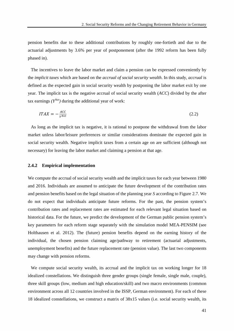
2. Social Security Reforms and the Changing Retirement Behavior in Germany
41
pension benefits due to these additional contributions by roughly one-fortieth and due to the
actuarial adjustments by 3.6% per year of postponement (after the 1992 reform has been fully
phased in).
The incentives to leave the labor market and claim a pension can be expressed conveniently by
the implicit taxes which are based on the accrual of social security wealth. In this study, accrual is
defined as the expected gain in social security wealth by postponing the labor market exit by one
year. The implicit tax is the negative accrual of social security wealth (ACC) divided by the after
tax earnings (YNet) during the additional year of work:
𝐼𝐼𝐼𝐼𝐼𝐼𝐼𝐼 = − 𝐴𝐴𝐴𝐴𝐴𝐴𝑌𝑌𝑁𝑁𝑁𝑁𝑁𝑁
(2.2)
As long as the implicit tax is negative, it is rational to postpone the withdrawal from the labor
market unless labor/leisure preferences or similar considerations dominate the expected gain in
social security wealth. Negative implicit taxes from a certain age on are sufficient (although not
necessary) for leaving the labor market and claiming a pension at that age.
2.4.2 Empirical implementation
We compute the accrual of social security wealth and the implicit taxes for each year between 1980
and 2016. Individuals are assumed to anticipate the future development of the contribution rates
and pension benefits based on the legal situation of the planning year S according to Figure 2.7. We
do not expect that individuals anticipate future reforms. For the past, the pension system’s
contribution rates and replacement rates are estimated for each relevant legal situation based on
historical data. For the future, we predict the development of the German public pension system’s
key parameters for each reform stage separately with the simulation model MEA-PENSIM (see
Holthausen et al. 2012). The (future) pension benefits depend on the earning history of the
individual, the chosen pension claiming age/pathway to retirement (actuarial adjustments,
unemployment benefits) and the future replacement rate (pension value). The last two components
may change with pension reforms.
We compute social security wealth, its accrual and the implicit tax on working longer for 18
idealized constellations. We distinguish three gender groups (single female, single male, couple),
three skill groups (low, medium and high education/skill) and two macro environments (common
environment across all 12 countries involved in the ISSP, German environment). For each of these
18 idealized constellations, we construct a matrix of 38x15 values (i.e. social security wealth, its
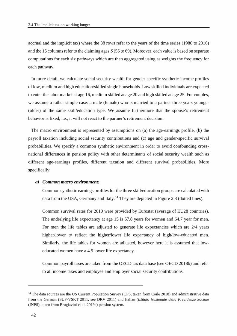
2.4 The implicit tax on working longer
42
accrual and the implicit tax) where the 38 rows refer to the years of the time series (1980 to 2016)
and the 15 columns refer to the claiming ages S (55 to 69). Moreover, each value is based on separate
computations for each six pathways which are then aggregated using as weights the frequency for
each pathway.
In more detail, we calculate social security wealth for gender-specific synthetic income profiles
of low, medium and high education/skilled single households. Low skilled individuals are expected
to enter the labor market at age 16, medium skilled at age 20 and high skilled at age 25. For couples,
we assume a rather simple case: a male (female) who is married to a partner three years younger
(older) of the same skill/education type. We assume furthermore that the spouse’s retirement
behavior is fixed, i.e., it will not react to the partner’s retirement decision.
The macro environment is represented by assumptions on (a) the age-earnings profile, (b) the
payroll taxation including social security contributions and (c) age and gender-specific survival
probabilities. We specify a common synthetic environment in order to avoid confounding cross-
national differences in pension policy with other determinants of social security wealth such as
different age-earnings profiles, different taxation and different survival probabilities. More
specifically:
a) Common macro environment:
Common synthetic earnings profiles for the three skill/education groups are calculated with
data from the USA, Germany and Italy.14 They are depicted in Figure 2.8 (dotted lines).
Common survival rates for 2010 were provided by Eurostat (average of EU28 countries).
The underlying life expectancy at age 15 is 67.8 years for women and 64.7 year for men.
For men the life tables are adjusted to generate life expectancies which are 2/4 years
higher/lower to reflect the higher/lower life expectancy of high/low-educated men.
Similarly, the life tables for women are adjusted, however here it is assumed that low-
educated women have a 4.5 lower life expectancy.
Common payroll taxes are taken from the OECD tax data base (see OECD 2018b) and refer
to all income taxes and employee and employer social security contributions.
14 The data sources are the US Current Population Survey (CPS, taken from Coile 2018) and administrative data from the German (SUF-VSKT 2011, see DRV 2011) and Italian (Istituto Nazionale della Previdenza Sociale (INPS), taken from Brugiavini et al. 2019a) pension system.
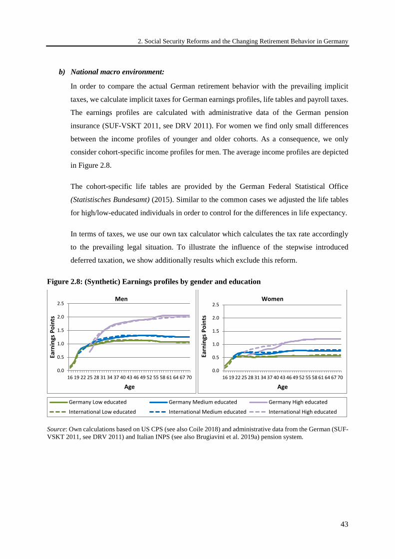
2. Social Security Reforms and the Changing Retirement Behavior in Germany
43
b) National macro environment:
In order to compare the actual German retirement behavior with the prevailing implicit
taxes, we calculate implicit taxes for German earnings profiles, life tables and payroll taxes.
The earnings profiles are calculated with administrative data of the German pension
insurance (SUF-VSKT 2011, see DRV 2011). For women we find only small differences
between the income profiles of younger and older cohorts. As a consequence, we only
consider cohort-specific income profiles for men. The average income profiles are depicted
in Figure 2.8.
The cohort-specific life tables are provided by the German Federal Statistical Office
(Statistisches Bundesamt) (2015). Similar to the common cases we adjusted the life tables
for high/low-educated individuals in order to control for the differences in life expectancy.
In terms of taxes, we use our own tax calculator which calculates the tax rate accordingly
to the prevailing legal situation. To illustrate the influence of the stepwise introduced
deferred taxation, we show additionally results which exclude this reform.
Figure 2.8: (Synthetic) Earnings profiles by gender and education
Source: Own calculations based on US CPS (see also Coile 2018) and administrative data from the German (SUF-VSKT 2011, see DRV 2011) and Italian INPS (see also Brugiavini et al. 2019a) pension system.
0.0
0.5
1.0
1.5
2.0
2.5
16 19 22 25 28 31 34 37 40 43 46 49 52 55 58 61 64 67 70
Earn
ings
Poi
nts
Age
Men
0.0
0.5
1.0
1.5
2.0
2.5
16 19 22 25 28 31 34 37 40 43 46 49 52 55 58 61 64 67 70
Earn
ings
Poi
nts
Age
Women
Germany Low educated Germany Medium educated Germany High educated
International Low educated International Medium educated International High educated
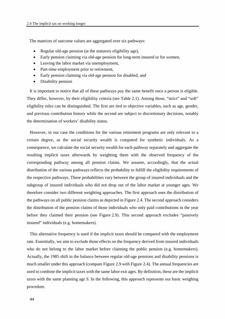
2.4 The implicit tax on working longer
44
The matrices of outcome values are aggregated over six pathways:
• Regular old-age pension (at the statutory eligibility age), • Early pension claiming via old-age pension for long-term insured or for women, • Leaving the labor market via unemployment, • Part-time employment prior to retirement, • Early pension claiming via old-age pension for disabled, and • Disability pension
It is important to notice that all of these pathways pay the same benefit once a person is eligible.
They differ, however, by their eligibility criteria (see Table 2.1). Among those, “strict” and “soft”
eligibility rules can be distinguished. The first are tied to objective variables, such as age, gender,
and previous contribution history while the second are subject to discretionary decisions, notably
the determination of workers’ disability status.
However, in our case the conditions for the various retirement programs are only relevant to a
certain degree, as the social security wealth is computed for synthetic individuals. As a
consequence, we calculate the social security wealth for each pathway separately and aggregate the
resulting implicit taxes afterwards by weighting them with the observed frequency of the
corresponding pathway among all pension claims. We assume, accordingly, that the actual
distribution of the various pathways reflects the probability to fulfill the eligibility requirements of
the respective pathways. These probabilities vary between the group of insured individuals and the
subgroup of insured individuals who did not drop out of the labor market at younger ages. We
therefore consider two different weighting approaches. The first approach uses the distribution of
the pathways on all public pension claims as depicted in Figure 2.4. The second approach considers
the distribution of the pension claims of those individuals who only paid contributions in the year
before they claimed their pension (see Figure 2.9). This second approach excludes “passively
insured” individuals (e.g. homemakers).
This alternative frequency is used if the implicit taxes should be compared with the employment
rate. Essentially, we aim to exclude those effects on the frequency derived from insured individuals
who do not belong to the labor market before claiming the public pension (e.g. homemakers).
Actually, the 1985 shift in the balance between regular old-age pensions and disability pensions is
much smaller under this approach (compare Figure 2.9 with Figure 2.4). The annual frequencies are
used to combine the implicit taxes with the same labor exit ages. By definition, these are the implicit
taxes with the same planning age S. In the following, this approach represents our basic weighing
procedure.
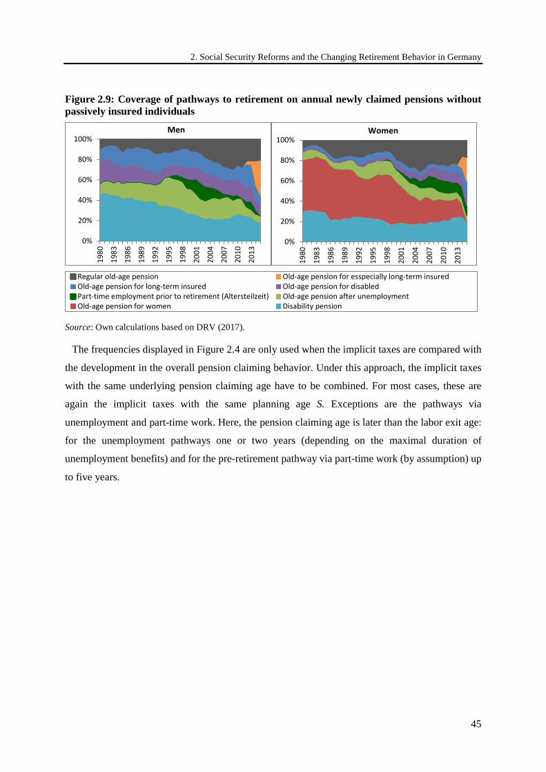
2. Social Security Reforms and the Changing Retirement Behavior in Germany
45
Figure 2.9: Coverage of pathways to retirement on annual newly claimed pensions without passively insured individuals
Source: Own calculations based on DRV (2017).
The frequencies displayed in Figure 2.4 are only used when the implicit taxes are compared with
the development in the overall pension claiming behavior. Under this approach, the implicit taxes
with the same underlying pension claiming age have to be combined. For most cases, these are
again the implicit taxes with the same planning age S. Exceptions are the pathways via
unemployment and part-time work. Here, the pension claiming age is later than the labor exit age:
for the unemployment pathways one or two years (depending on the maximal duration of
unemployment benefits) and for the pre-retirement pathway via part-time work (by assumption) up
to five years.
0%
20%
40%
60%
80%
100%
1980
1983
1986
1989
1992
1995
1998
2001
2004
2007
2010
2013
Men
0%
20%
40%
60%
80%
100%
1980
1983
1986
1989
1992
1995
1998
2001
2004
2007
2010
2013
Women
Regular old-age pension Old-age pension for esspecially long-term insuredOld-age pension for long-term insured Old-age pension for disabledPart-time employment prior to retirement (Altersteilzeit) Old-age pension after unemploymentOld-age pension for women Disability pension

2.5 Results
46
2.5 Results
In the following, we will present the results of our calculations in a stepwise fashion. Section 2.5.1
presents individualized replacement rates and social security wealth, i.e., the elements from which
the implicit tax will be computed, on a scale more often used in the economics literature than the
German-specific “standardized replacement rates” in Section 2.3 (Table 2.2). For comparability, we
apply the German payroll taxes.
In Section 2.5.2, we introduce the common macro environment. We first present general outcome
variables such as replacement rate, social security wealth and its accrual. Section 2.5.3 follows with
the implicit tax on working longer for median educated men, women and couples. Section 2.5.4
shows how these implicit taxes vary between different skill groups.
Section 2.5.5 uses the differences between the common environment and the national case for a
discussion how the implicit taxes depend on specific national taxation, income profiles and life
tables.
Finally, Section 2.5.6 and Section 2.5.7 are devoted to a graphical juxtaposition of our computed
implicit taxes with the actual development of employment and the changes in the distribution of the
pension claiming age.
2.5.1 Replacement rates and social security wealth, scaled for Germany
2.5.1.1 Replacement rate
The standardized replacement rates shown in Table 2.2 of a pensioner with constant average
earnings over the entire work life do not reflect actual earnings profiles which typically increase
with age. Moreover, these standardized replacement rates do not take the introduction of the
deferred taxation on pension benefits into account. As a consequence, we analyze in the following
individualized net replacement rates (pension benefits as share of last earnings by the types of
individuals and households defined in the previous section) which were computed in the calculation
process of the implicit taxes.
In order to maintain some comparability to the official German figures, the calculations in this
section are based on the tax rate calculations of the German macro environment (see Section 2.4)
but use the income profiles and survival probabilities of the common macro environment. The most
critical difference is the fact that the common taxation does not only tax labor income but also
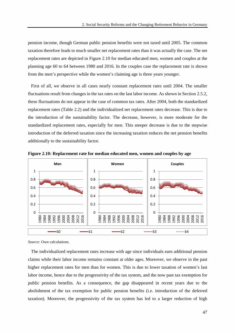
2. Social Security Reforms and the Changing Retirement Behavior in Germany
47
pension income, though German public pension benefits were not taxed until 2005. The common
taxation therefore leads to much smaller net replacement rates than it was actually the case. The net
replacement rates are depicted in Figure 2.10 for median educated men, women and couples at the
planning age 60 to 64 between 1980 and 2016. In the couples case the replacement rate is shown
from the men’s perspective while the women’s claiming age is three years younger.
First of all, we observe in all cases nearly constant replacement rates until 2004. The smaller
fluctuations result from changes in the tax rates on the last labor income. As shown in Section 2.5.2,
these fluctuations do not appear in the case of common tax rates. After 2004, both the standardized
replacement rates (Table 2.2) and the individualized net replacement rates decrease. This is due to
the introduction of the sustainability factor. The decrease, however, is more moderate for the
standardized replacement rates, especially for men. This steeper decrease is due to the stepwise
introduction of the deferred taxation since the increasing taxation reduces the net pension benefits
additionally to the sustainability factor.
Figure 2.10: Replacement rate for median educated men, women and couples by age
Source: Own calculations.
The individualized replacement rates increase with age since individuals earn additional pension
claims while their labor income remains constant at older ages. Moreover, we observe in the past
higher replacement rates for men than for women. This is due to lower taxation of women’s last
labor income, hence due to the progressivity of the tax system, and the now past tax exemption for
public pension benefits. As a consequence, the gap disappeared in recent years due to the
abolishment of the tax exemption for public pension benefits (i.e. introduction of the deferred
taxation). Moreover, the progressivity of the tax system has led to a larger reduction of high
0
0.2
0.4
0.6
0.8
1
1980
1984
1988
1992
1996
2000
2004
2008
2012
2016
Men
0
0.2
0.4
0.6
0.8
1
1980
1984
1988
1992
1996
2000
2004
2008
2012
2016
Women
0
0.2
0.4
0.6
0.8
1
1980
1984
1988
1992
1996
2000
2004
2008
2012
2016
Couples
00.20.40.60.81 60 61 62 63 64
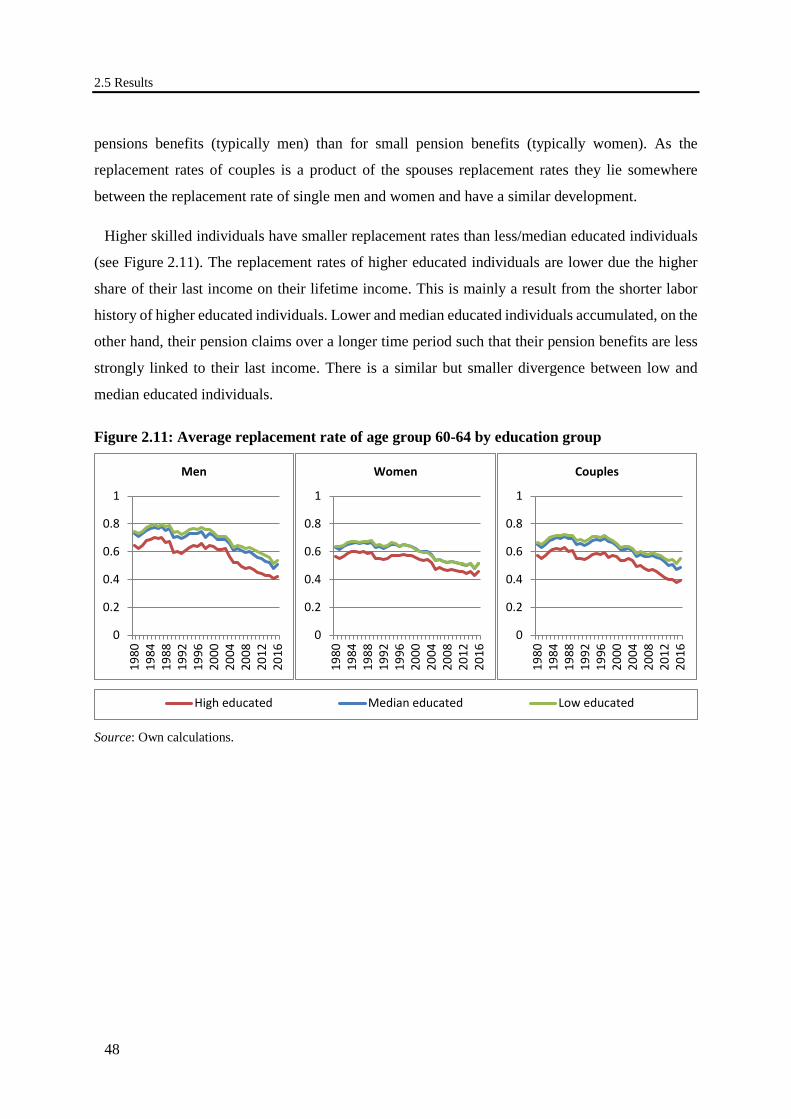
2.5 Results
48
pensions benefits (typically men) than for small pension benefits (typically women). As the
replacement rates of couples is a product of the spouses replacement rates they lie somewhere
between the replacement rate of single men and women and have a similar development.
Higher skilled individuals have smaller replacement rates than less/median educated individuals
(see Figure 2.11). The replacement rates of higher educated individuals are lower due the higher
share of their last income on their lifetime income. This is mainly a result from the shorter labor
history of higher educated individuals. Lower and median educated individuals accumulated, on the
other hand, their pension claims over a longer time period such that their pension benefits are less
strongly linked to their last income. There is a similar but smaller divergence between low and
median educated individuals.
Figure 2.11: Average replacement rate of age group 60-64 by education group
Source: Own calculations.
0
0.2
0.4
0.6
0.8
1
1980
1984
1988
1992
1996
2000
2004
2008
2012
2016
Men
0
0.2
0.4
0.6
0.8
1
1980
1984
1988
1992
1996
2000
2004
2008
2012
2016
Women
0
0.2
0.4
0.6
0.8
1
1980
1984
1988
1992
1996
2000
2004
2008
2012
2016
Couples
High educated Median educated Low educated
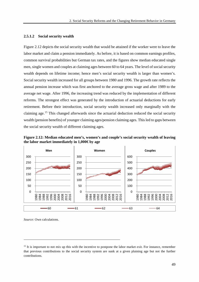
2. Social Security Reforms and the Changing Retirement Behavior in Germany
49
2.5.1.2 Social security wealth
Figure 2.12 depicts the social security wealth that would be attained if the worker were to leave the
labor market and claim a pension immediately. As before, it is based on common earnings profiles,
common survival probabilities but German tax rates, and the figures show median educated single
men, single women and couples at claiming ages between 60 to 64 years. The level of social security
wealth depends on lifetime income; hence men’s social security wealth is larger than women’s.
Social security wealth increased for all groups between 1980 and 1996. The growth rate reflects the
annual pension increase which was first anchored to the average gross wage and after 1989 to the
average net wage. After 1996, the increasing trend was reduced by the implementation of different
reforms. The strongest effect was generated by the introduction of actuarial deductions for early
retirement. Before their introduction, social security wealth increased only marginally with the
claiming age.15 This changed afterwards since the actuarial deduction reduced the social security
wealth (pension benefits) of younger claiming ages/pension claiming ages. This led to gaps between
the social security wealth of different claiming ages.
Figure 2.12: Median educated men’s, women’s and couple’s social security wealth of leaving the labor market immediately in 1,000€ by age
Source: Own calculations.
15 It is important to not mix up this with the incentive to postpone the labor market exit. For instance, remember that previous contributions to the social security system are sunk at a given plaining age but not the further contributions.
0
50
100
150
200
250
300
1980
1984
1988
1992
1996
2000
2004
2008
2012
2016
Men
0
50
100
150
200
250
300
1980
1984
1988
1992
1996
2000
2004
2008
2012
2016
Women
0
100
200
300
400
500
600
1980
1984
1988
1992
1996
2000
2004
2008
2012
2016
Couples
00.20.40.60.81 60 61 62 63 64
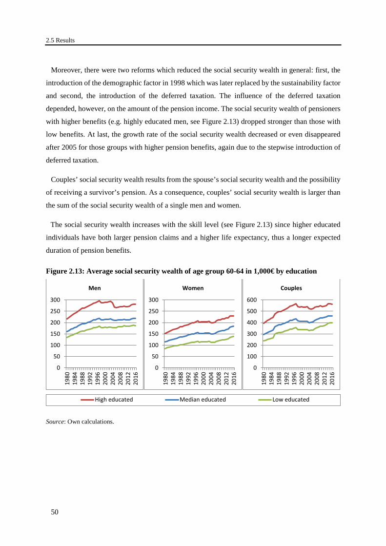
2.5 Results
50
Moreover, there were two reforms which reduced the social security wealth in general: first, the
introduction of the demographic factor in 1998 which was later replaced by the sustainability factor
and second, the introduction of the deferred taxation. The influence of the deferred taxation
depended, however, on the amount of the pension income. The social security wealth of pensioners
with higher benefits (e.g. highly educated men, see Figure 2.13) dropped stronger than those with
low benefits. At last, the growth rate of the social security wealth decreased or even disappeared
after 2005 for those groups with higher pension benefits, again due to the stepwise introduction of
deferred taxation.
Couples’ social security wealth results from the spouse’s social security wealth and the possibility
of receiving a survivor’s pension. As a consequence, couples’ social security wealth is larger than
the sum of the social security wealth of a single men and women.
The social security wealth increases with the skill level (see Figure 2.13) since higher educated
individuals have both larger pension claims and a higher life expectancy, thus a longer expected
duration of pension benefits.
Figure 2.13: Average social security wealth of age group 60-64 in 1,000€ by education
Source: Own calculations.
0
50
100
150
200
250
300
1980
1984
1988
1992
1996
2000
2004
2008
2012
2016
Men
0
50
100
150
200
250
300
1980
1984
1988
1992
1996
2000
2004
2008
2012
2016
Women
0
100
200
300
400
500
600
1980
1984
1988
1992
1996
2000
2004
2008
2012
2016
Couples
High educated Median educated Low educated
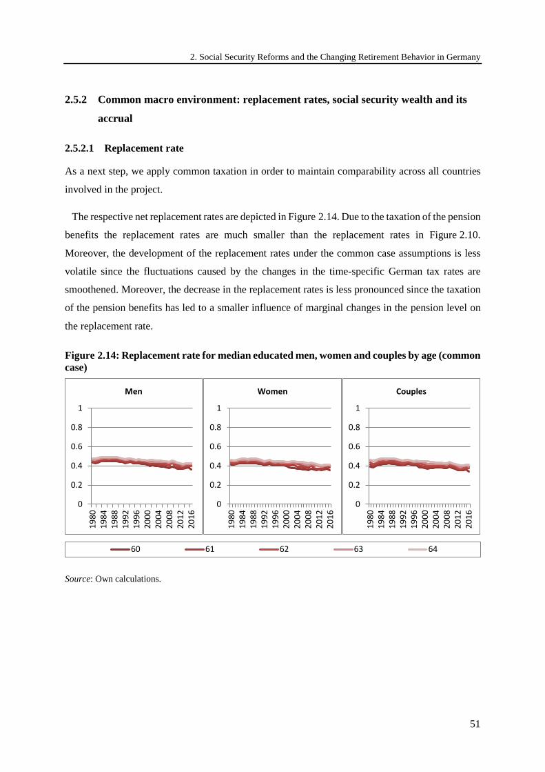
2. Social Security Reforms and the Changing Retirement Behavior in Germany
51
2.5.2 Common macro environment: replacement rates, social security wealth and its
accrual
2.5.2.1 Replacement rate
As a next step, we apply common taxation in order to maintain comparability across all countries
involved in the project.
The respective net replacement rates are depicted in Figure 2.14. Due to the taxation of the pension
benefits the replacement rates are much smaller than the replacement rates in Figure 2.10.
Moreover, the development of the replacement rates under the common case assumptions is less
volatile since the fluctuations caused by the changes in the time-specific German tax rates are
smoothened. Moreover, the decrease in the replacement rates is less pronounced since the taxation
of the pension benefits has led to a smaller influence of marginal changes in the pension level on
the replacement rate.
Figure 2.14: Replacement rate for median educated men, women and couples by age (common case)
Source: Own calculations.
0
0.2
0.4
0.6
0.8
1
1980
1984
1988
1992
1996
2000
2004
2008
2012
2016
Men
0
0.2
0.4
0.6
0.8
1
1980
1984
1988
1992
1996
2000
2004
2008
2012
2016
Women
0
0.2
0.4
0.6
0.8
1
1980
1984
1988
1992
1996
2000
2004
2008
2012
2016
Couples
00.20.40.60.81 60 61 62 63 64
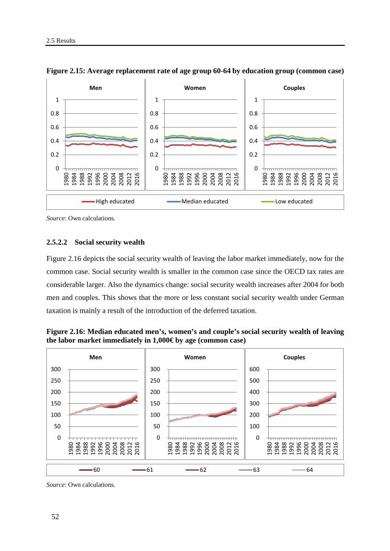
2.5 Results
52
Figure 2.15: Average replacement rate of age group 60-64 by education group (common case)
Source: Own calculations.
2.5.2.2 Social security wealth
Figure 2.16 depicts the social security wealth of leaving the labor market immediately, now for the
common case. Social security wealth is smaller in the common case since the OECD tax rates are
considerable larger. Also the dynamics change: social security wealth increases after 2004 for both
men and couples. This shows that the more or less constant social security wealth under German
taxation is mainly a result of the introduction of the deferred taxation.
Figure 2.16: Median educated men’s, women’s and couple’s social security wealth of leaving the labor market immediately in 1,000€ by age (common case)
Source: Own calculations.
0
0.2
0.4
0.6
0.8
1
1980
1984
1988
1992
1996
2000
2004
2008
2012
2016
Men
0
0.2
0.4
0.6
0.8
1
1980
1984
1988
1992
1996
2000
2004
2008
2012
2016
Women
0
0.2
0.4
0.6
0.8
1
1980
1984
1988
1992
1996
2000
2004
2008
2012
2016
Couples
High educated Median educated Low educated
0
50
100
150
200
250
300
1980
1984
1988
1992
1996
2000
2004
2008
2012
2016
Men
0
50
100
150
200
250
300
1980
1984
1988
1992
1996
2000
2004
2008
2012
2016
Women
0
100
200
300
400
500
600
1980
1984
1988
1992
1996
2000
2004
2008
2012
2016
Couples
00.20.40.60.81 60 61 62 63 64
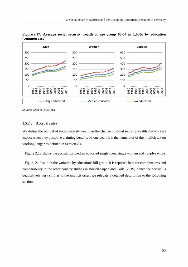
2. Social Security Reforms and the Changing Retirement Behavior in Germany
53
Figure 2.17: Average social security wealth of age group 60-64 in 1,000€ by education (common case)
Source: Own calculations.
2.5.2.3 Accrual rates
We define the accrual of social security wealth as the change in social security wealth that workers
expect when they postpone claiming benefits by one year. It is the numerator of the implicit tax on
working longer as defined in Section 2.4.
Figure 2.18 shows the accrual for median educated single men, single women and couples while
Figure 2.19 studies the variation by education/skill group. It is reported here for completeness and
comparability to the other country studies in Börsch-Supan and Coile (2019). Since the accrual is
qualitatively very similar to the implicit taxes, we relegate a detailed description to the following
section.
0
50
100
150
200
250
300
1980
1984
1988
1992
1996
2000
2004
2008
2012
2016
Men
0
50
100
150
200
250
300
1980
1984
1988
1992
1996
2000
2004
2008
2012
2016
Women
0
100
200
300
400
500
600
1980
1984
1988
1992
1996
2000
2004
2008
2012
2016
Couples
High educated Median educated Low educated
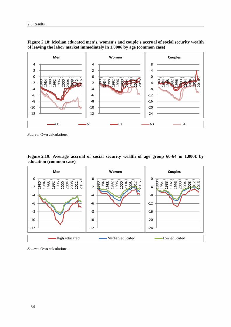
2.5 Results
54
Figure 2.18: Median educated men’s, women’s and couple’s accrual of social security wealth of leaving the labor market immediately in 1,000€ by age (common case)
Source: Own calculations.
Figure 2.19: Average accrual of social security wealth of age group 60-64 in 1,000€ by education (common case)
Source: Own calculations.
-12
-10
-8
-6
-4
-2
0
2
4
1980
1984
1988
1992
1996
2000
2004
2008
2012
2016
Men
-12
-10
-8
-6
-4
-2
0
2
4
1980
1984
1988
1992
1996
2000
2004
2008
2012
2016
Women
-24
-20
-16
-12
-8
-4
0
4
8
1980
1984
1988
1992
1996
2000
2004
2008
2012
2016
Couples
00.20.40.60.81 60 61 62 63 64
-12
-10
-8
-6
-4
-2
0
1980
1984
1988
1992
1996
2000
2004
2008
2012
2016
Men
-12
-10
-8
-6
-4
-2
0
1980
1984
1988
1992
1996
2000
2004
2008
2012
2016
Women
-24
-20
-16
-12
-8
-4
0
1980
1984
1988
1992
1996
2000
2004
2008
2012
2016
Couples
High educated Median educated Low educated
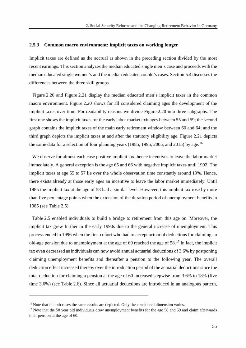
2. Social Security Reforms and the Changing Retirement Behavior in Germany
55
2.5.3 Common macro environment: implicit taxes on working longer
Implicit taxes are defined as the accrual as shown in the preceding section divided by the most
recent earnings. This section analyzes the median educated single men’s case and proceeds with the
median educated single women’s and the median educated couple’s cases. Section 5.4 discusses the
differences between the three skill groups.
Figure 2.20 and Figure 2.21 display the median educated men’s implicit taxes in the common
macro environment. Figure 2.20 shows for all considered claiming ages the development of the
implicit taxes over time. For readability reasons we divide Figure 2.20 into three subgraphs. The
first one shows the implicit taxes for the early labor market exit ages between 55 and 59; the second
graph contains the implicit taxes of the main early retirement window between 60 and 64; and the
third graph depicts the implicit taxes at and after the statutory eligibility age. Figure 2.21 depicts
the same data for a selection of four planning years (1985, 1995, 2005, and 2015) by age.16
We observe for almost each case positive implicit tax, hence incentives to leave the labor market
immediately. A general exception is the age 65 and 66 with negative implicit taxes until 1992. The
implicit taxes at age 55 to 57 lie over the whole observation time constantly around 19%. Hence,
there exists already at those early ages an incentive to leave the labor market immediately. Until
1985 the implicit tax at the age of 58 had a similar level. However, this implicit tax rose by more
than five percentage points when the extension of the duration period of unemployment benefits in
1985 (see Table 2.5).
Table 2.5 enabled individuals to build a bridge to retirement from this age on. Moreover, the
implicit tax grew further in the early 1990s due to the general increase of unemployment. This
process ended in 1996 when the first cohort who had to accept actuarial deductions for claiming an
old-age pension due to unemployment at the age of 60 reached the age of 58.17 In fact, the implicit
tax even decreased as individuals can now avoid annual actuarial deductions of 3.6% by postponing
claiming unemployment benefits and thereafter a pension to the following year. The overall
deduction effect increased thereby over the introduction period of the actuarial deductions since the
total deduction for claiming a pension at the age of 60 increased stepwise from 3.6% to 18% (five
time 3.6%) (see Table 2.6). Since all actuarial deductions are introduced in an analogous pattern,
16 Note that in both cases the same results are depicted. Only the considered dimension varies. 17 Note that the 58 year old individuals draw unemployment benefits for the age 58 and 59 and claim afterwards their pension at the age of 60.
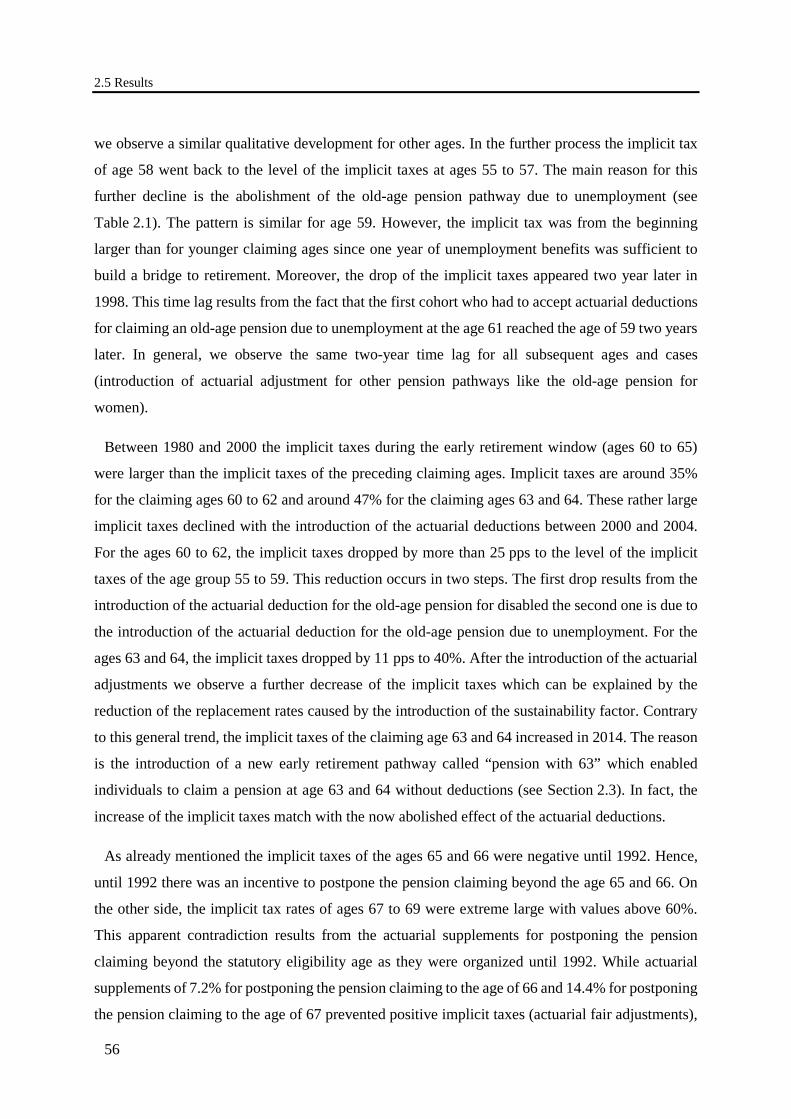
2.5 Results
56
we observe a similar qualitative development for other ages. In the further process the implicit tax
of age 58 went back to the level of the implicit taxes at ages 55 to 57. The main reason for this
further decline is the abolishment of the old-age pension pathway due to unemployment (see
Table 2.1). The pattern is similar for age 59. However, the implicit tax was from the beginning
larger than for younger claiming ages since one year of unemployment benefits was sufficient to
build a bridge to retirement. Moreover, the drop of the implicit taxes appeared two year later in
1998. This time lag results from the fact that the first cohort who had to accept actuarial deductions
for claiming an old-age pension due to unemployment at the age 61 reached the age of 59 two years
later. In general, we observe the same two-year time lag for all subsequent ages and cases
(introduction of actuarial adjustment for other pension pathways like the old-age pension for
women).
Between 1980 and 2000 the implicit taxes during the early retirement window (ages 60 to 65)
were larger than the implicit taxes of the preceding claiming ages. Implicit taxes are around 35%
for the claiming ages 60 to 62 and around 47% for the claiming ages 63 and 64. These rather large
implicit taxes declined with the introduction of the actuarial deductions between 2000 and 2004.
For the ages 60 to 62, the implicit taxes dropped by more than 25 pps to the level of the implicit
taxes of the age group 55 to 59. This reduction occurs in two steps. The first drop results from the
introduction of the actuarial deduction for the old-age pension for disabled the second one is due to
the introduction of the actuarial deduction for the old-age pension due to unemployment. For the
ages 63 and 64, the implicit taxes dropped by 11 pps to 40%. After the introduction of the actuarial
adjustments we observe a further decrease of the implicit taxes which can be explained by the
reduction of the replacement rates caused by the introduction of the sustainability factor. Contrary
to this general trend, the implicit taxes of the claiming age 63 and 64 increased in 2014. The reason
is the introduction of a new early retirement pathway called “pension with 63” which enabled
individuals to claim a pension at age 63 and 64 without deductions (see Section 2.3). In fact, the
increase of the implicit taxes match with the now abolished effect of the actuarial deductions.
As already mentioned the implicit taxes of the ages 65 and 66 were negative until 1992. Hence,
until 1992 there was an incentive to postpone the pension claiming beyond the age 65 and 66. On
the other side, the implicit tax rates of ages 67 to 69 were extreme large with values above 60%.
This apparent contradiction results from the actuarial supplements for postponing the pension
claiming beyond the statutory eligibility age as they were organized until 1992. While actuarial
supplements of 7.2% for postponing the pension claiming to the age of 66 and 14.4% for postponing
the pension claiming to the age of 67 prevented positive implicit taxes (actuarial fair adjustments),
2. Social Security Reforms and the Changing Retirement Behavior in Germany
57
there were no actuarial supplements for postponing the pension claiming beyond age 67. As the
general actuarial supplements of six percent were introduced in 1992 the implicit taxes dropped
consequently considerable for the claiming ages 67 to 69. All in all, we observe a reduction of more
than 30 pps. The reduction was, thereby, larger for later claiming ages. However, the actuarial
supplements for postponing the pension claiming at the age of 65 and 66 were reduced at the same
time the implicit taxes of those claiming ages started to increase by approximately 20 pps which
corresponds to the reduction of the former actuarial supplements. Similar to the claiming ages 60
to 64, the implicit taxes of the claiming ages 65 to 69 started to decrease in 2004 due to the
introduction of the sustainability factor. For the most claiming ages, this decrease continued until
today. An exception includes the claiming age 65 for which the implicit tax started to increase in
2012. The explanation for this opposite development lies in the increase of the statutory eligibility
age from 65 to 67. The incentive to leave the labor market increases due to the fact that an individual
does not anymore receive higher actuarial supplements for postponing the pension claiming beyond
the statutory eligibility age but prevents only the smaller actuarial deduction for claiming a pension
before his statutory eligibility age. Once the transition to the higher statutory eligibility age is
completed, the implicit tax of the claiming age 65 should have risen to a similar level as of the
implicit taxes of the claiming ages 63 and 64.
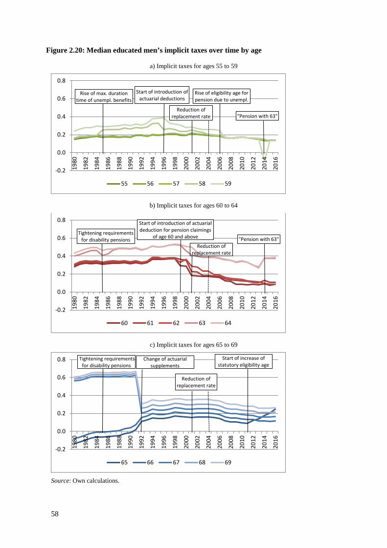
58
Figure 2.20: Median educated men’s implicit taxes over time by age
a) Implicit taxes for ages 55 to 59
b) Implicit taxes for ages 60 to 64
c) Implicit taxes for ages 65 to 69
Source: Own calculations.
-0.2
0.0
0.2
0.4
0.6
0.819
80
1982
1984
1986
1988
1990
1992
1994
1996
1998
2000
2002
2004
2006
2008
2010
2012
2014
2016
55 56 57 58 59
Rise of max. duration time of unempl. benefits
Start of introduction of actuarial deductions
Rise of eligibility age for pension due to unempl.
Reduction of replacement rate "Pension with 63"
-0.2
0.0
0.2
0.4
0.6
0.8
1980
1982
1984
1986
1988
1990
1992
1994
1996
1998
2000
2002
2004
2006
2008
2010
2012
2014
2016
60 61 62 63 64
Tightening requirements for disability pensions
Start of introduction of actuarial deduction for pension claimings
of age 60 and above "Pension with 63"Reduction of
replacement rate
-0.2
0.0
0.2
0.4
0.6
0.8
1980
1982
1984
1986
1988
1990
1992
1994
1996
1998
2000
2002
2004
2006
2008
2010
2012
2014
2016
65 66 67 68 69
Tightening requirements for disability pensions
Change of actuarial supplements
Start of increase of statutory eligibility age
Reduction of replacement rate
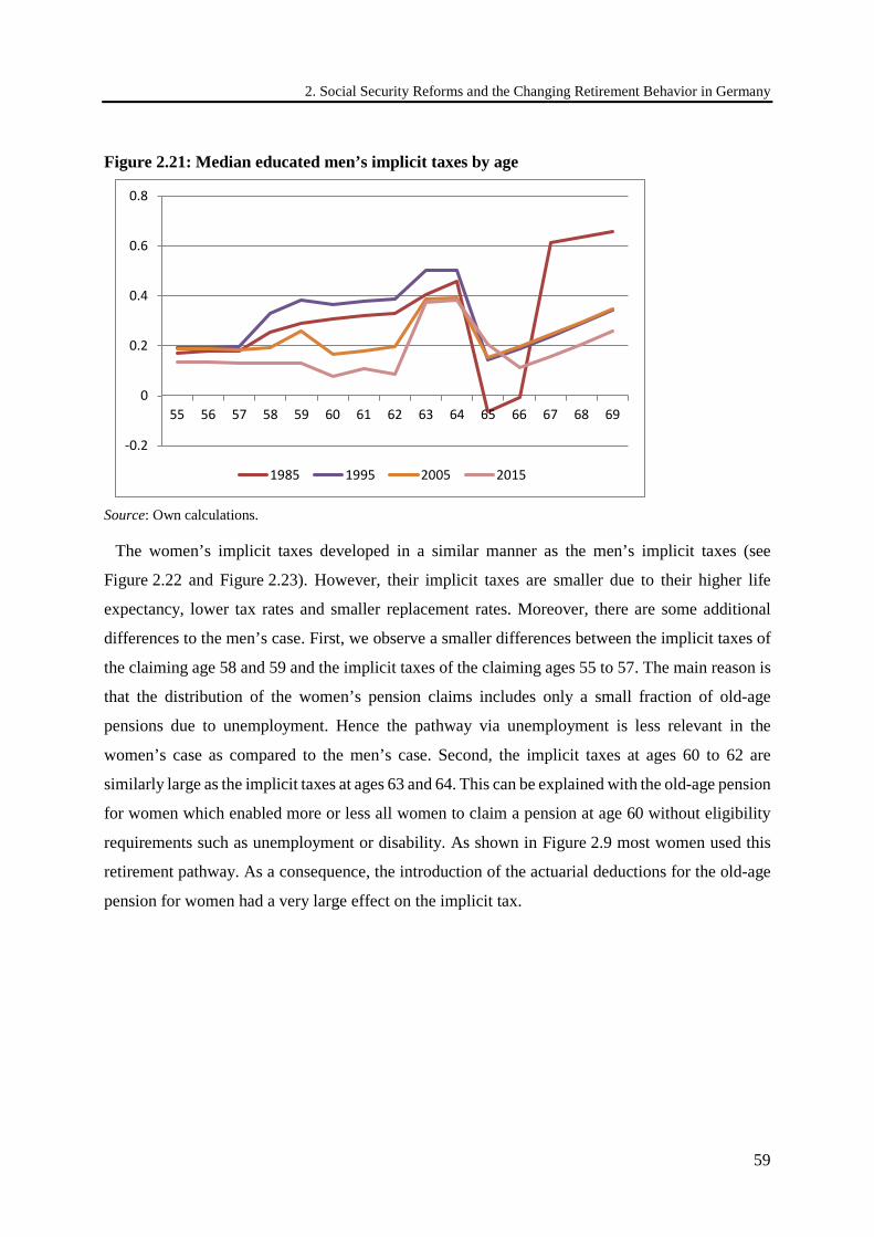
2. Social Security Reforms and the Changing Retirement Behavior in Germany
59
Figure 2.21: Median educated men’s implicit taxes by age
Source: Own calculations.
The women’s implicit taxes developed in a similar manner as the men’s implicit taxes (see
Figure 2.22 and Figure 2.23). However, their implicit taxes are smaller due to their higher life
expectancy, lower tax rates and smaller replacement rates. Moreover, there are some additional
differences to the men’s case. First, we observe a smaller differences between the implicit taxes of
the claiming age 58 and 59 and the implicit taxes of the claiming ages 55 to 57. The main reason is
that the distribution of the women’s pension claims includes only a small fraction of old-age
pensions due to unemployment. Hence the pathway via unemployment is less relevant in the
women’s case as compared to the men’s case. Second, the implicit taxes at ages 60 to 62 are
similarly large as the implicit taxes at ages 63 and 64. This can be explained with the old-age pension
for women which enabled more or less all women to claim a pension at age 60 without eligibility
requirements such as unemployment or disability. As shown in Figure 2.9 most women used this
retirement pathway. As a consequence, the introduction of the actuarial deductions for the old-age
pension for women had a very large effect on the implicit tax.
-0.2
0
0.2
0.4
0.6
0.8
55 56 57 58 59 60 61 62 63 64 65 66 67 68 69
1985 1995 2005 2015
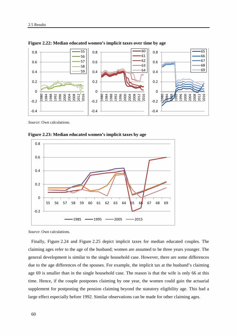
2.5 Results
60
Figure 2.22: Median educated women’s implicit taxes over time by age
Source: Own calculations.
Figure 2.23: Median educated women’s implicit taxes by age
Source: Own calculations.
Finally, Figure 2.24 and Figure 2.25 depict implicit taxes for median educated couples. The
claiming ages refer to the age of the husband; women are assumed to be three years younger. The
general development is similar to the single household case. However, there are some differences
due to the age differences of the spouses. For example, the implicit tax at the husband’s claiming
age 69 is smaller than in the single household case. The reason is that the wife is only 66 at this
time. Hence, if the couple postpones claiming by one year, the women could gain the actuarial
supplement for postponing the pension claiming beyond the statutory eligibility age. This had a
large effect especially before 1992. Similar observations can be made for other claiming ages.
-0.4
-0.2
0
0.2
0.4
0.6
0.8
1980
1984
1988
1992
1996
2000
2004
2008
2012
2016
5556575859
-0.4
-0.2
0
0.2
0.4
0.6
0.8
1980
1984
1988
1992
1996
2000
2004
2008
2012
2016
6061626364
-0.4
-0.2
0
0.2
0.4
0.6
0.8
1980
1984
1988
1992
1996
2000
2004
2008
2012
2016
6566676869
-0.2
0
0.2
0.4
0.6
0.8
55 56 57 58 59 60 61 62 63 64 65 66 67 68 69
1985 1995 2005 2015
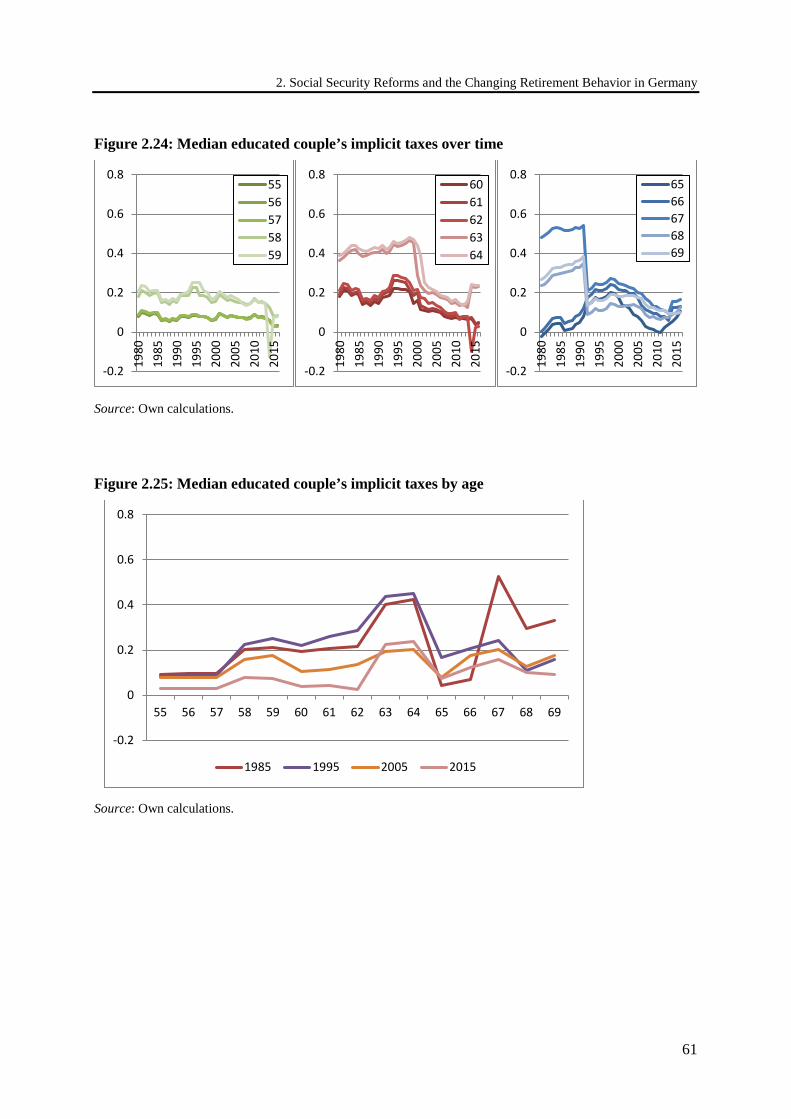
2. Social Security Reforms and the Changing Retirement Behavior in Germany
61
Figure 2.24: Median educated couple’s implicit taxes over time
Source: Own calculations.
Figure 2.25: Median educated couple’s implicit taxes by age
Source: Own calculations.
-0.2
0
0.2
0.4
0.6
0.8
1980
1985
1990
1995
2000
2005
2010
2015
5556575859
-0.2
0
0.2
0.4
0.6
0.8
1980
1985
1990
1995
2000
2005
2010
2015
6061626364
-0.2
0
0.2
0.4
0.6
0.8
1980
1985
1990
1995
2000
2005
2010
2015
6566676869
-0.2
0
0.2
0.4
0.6
0.8
55 56 57 58 59 60 61 62 63 64 65 66 67 68 69
1985 1995 2005 2015
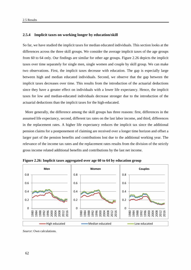
2.5 Results
62
2.5.4 Implicit taxes on working longer by education/skill
So far, we have studied the implicit taxes for median educated individuals. This section looks at the
differences across the three skill groups. We consider the average implicit taxes of the age groups
from 60 to 64 only. Our findings are similar for other age groups. Figure 2.26 depicts the implicit
taxes over time separately for single men, single women and couple by skill group. We can make
two observations. First, the implicit taxes decrease with education. The gap is especially large
between high and median educated individuals. Second, we observe that the gap between the
implicit taxes decreases over time. This results from the introduction of the actuarial deductions
since they have a greater effect on individuals with a lower life expectancy. Hence, the implicit
taxes for low and median-educated individuals decrease stronger due to the introduction of the
actuarial deductions than the implicit taxes for the high-educated.
More generally, the difference among the skill groups has three reasons: first, differences in the
assumed life expectancy, second, different tax rates on the last labor income, and third, differences
in the replacement rates. A higher life expectancy reduces the implicit tax since the additional
pension claims for a postponement of claiming are received over a longer time horizon and offset a
larger part of the pension benefits and contributions lost due to the additional working year. The
relevance of the income tax rates and the replacement rates results from the division of the strictly
gross income related additional benefits and contributions by the last net income.
Figure 2.26: Implicit taxes aggregated over age 60 to 64 by education group
Source: Own calculations.
0
0.2
0.4
0.6
0.8
1980
1984
1988
1992
1996
2000
2004
2008
2012
2016
Men
0
0.2
0.4
0.6
0.8
1980
1984
1988
1992
1996
2000
2004
2008
2012
2016
Women
0
0.2
0.4
0.6
0.8
1980
1984
1988
1992
1996
2000
2004
2008
2012
2016
Couples
High educated Median educated Low educated

2. Social Security Reforms and the Changing Retirement Behavior in Germany
63
2.5.5 German macro environment: the influence of changes in the taxation, cohort-
specific income profiles and survival probabilities
We now switch from the common macro environment to the German macro environment. We
discuss in which way taxation, cohort-specific income profiles and survival probabilities influence
the implicit taxes. We start with taxation, then proceed with analyzing the income profiles and close
with the survival probabilities.
Figure 2.27 depicts the average implicit taxes of single men, single women and couples at the
claiming ages 60 to 64 for different taxations of the gross pension and labor income. All figures are
aggregated over the three education groups. We consider three cases: first, the common taxation
used in the common macro environment; second, the German taxation according to our tax
calculator but without the introduction of the deferred taxation and finally German taxation with
deferred taxation. The income profiles and survival probabilities remain as before and are taken
from the common macro environment.18
Until 2000, we observe for each case smaller implicit taxes under the common taxation than under
the time-specific German taxation. The gap is larger for men than for women. It results from the
fact that under the common taxation not only is the labor income taxed, but also public pension
benefits. At the end of the 1990s, the gap becomes smaller and since 2000 the implicit taxes are
larger under the common taxation than under the German time-specific taxation (at least if we do
not consider the deferred taxation). This reversal is due to the introduction of the actuarial
deductions which reduce the gain of claiming a pension immediately.
We have already shown that the deferred taxation has had a large influence on the determinants
of the implicit taxes such as the replacement rate. Consequently, we also see a large reaction of the
implicit taxes to the introduction of the deferred taxation, see Figure 2.27. The deferred taxation led
to an increase of the implicit taxes for single men and couples. This effect is larger for higher
claiming ages and conceals most of the effects that we have observed in the previous section, e.g.
the effect of the “pension with 63” or the effect due to the increase of the statutory eligibility age.
That we do not observe an effect on the women’s implicit taxes results from their rather small
pension benefits and the large tax allowances which were granted at the beginning of the
18 Note that the last case corresponds to the case for which we had presented the replacement rates and social security wealth shown in Section 2.5.1.
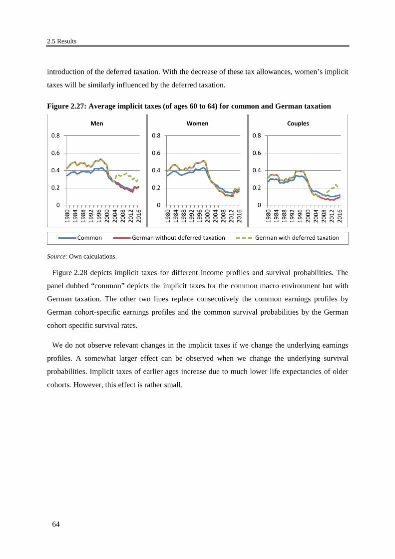
2.5 Results
64
introduction of the deferred taxation. With the decrease of these tax allowances, women’s implicit
taxes will be similarly influenced by the deferred taxation.
Figure 2.27: Average implicit taxes (of ages 60 to 64) for common and German taxation
Source: Own calculations.
Figure 2.28 depicts implicit taxes for different income profiles and survival probabilities. The
panel dubbed “common” depicts the implicit taxes for the common macro environment but with
German taxation. The other two lines replace consecutively the common earnings profiles by
German cohort-specific earnings profiles and the common survival probabilities by the German
cohort-specific survival rates.
We do not observe relevant changes in the implicit taxes if we change the underlying earnings
profiles. A somewhat larger effect can be observed when we change the underlying survival
probabilities. Implicit taxes of earlier ages increase due to much lower life expectancies of older
cohorts. However, this effect is rather small.
0
0.2
0.4
0.6
0.8
1980
1984
1988
1992
1996
2000
2004
2008
2012
2016
Men
0
0.2
0.4
0.6
0.8
1980
1984
1988
1992
1996
2000
2004
2008
2012
2016
Women
0
0.2
0.4
0.6
0.8
1980
1984
1988
1992
1996
2000
2004
2008
2012
2016
Couples
Common German without deferred taxation German with deferred taxation
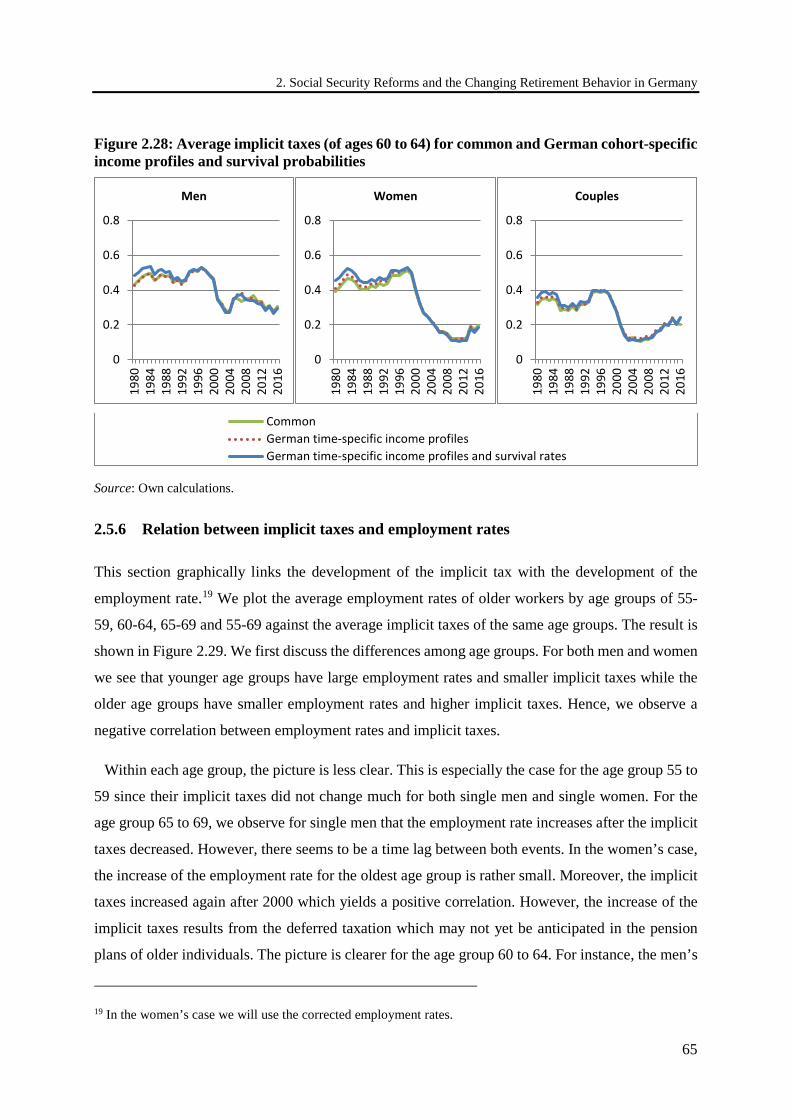
2. Social Security Reforms and the Changing Retirement Behavior in Germany
65
Figure 2.28: Average implicit taxes (of ages 60 to 64) for common and German cohort-specific income profiles and survival probabilities
Source: Own calculations.
2.5.6 Relation between implicit taxes and employment rates
This section graphically links the development of the implicit tax with the development of the
employment rate.19 We plot the average employment rates of older workers by age groups of 55-
59, 60-64, 65-69 and 55-69 against the average implicit taxes of the same age groups. The result is
shown in Figure 2.29. We first discuss the differences among age groups. For both men and women
we see that younger age groups have large employment rates and smaller implicit taxes while the
older age groups have smaller employment rates and higher implicit taxes. Hence, we observe a
negative correlation between employment rates and implicit taxes.
Within each age group, the picture is less clear. This is especially the case for the age group 55 to
59 since their implicit taxes did not change much for both single men and single women. For the
age group 65 to 69, we observe for single men that the employment rate increases after the implicit
taxes decreased. However, there seems to be a time lag between both events. In the women’s case,
the increase of the employment rate for the oldest age group is rather small. Moreover, the implicit
taxes increased again after 2000 which yields a positive correlation. However, the increase of the
implicit taxes results from the deferred taxation which may not yet be anticipated in the pension
plans of older individuals. The picture is clearer for the age group 60 to 64. For instance, the men’s
19 In the women’s case we will use the corrected employment rates.
0
0.2
0.4
0.6
0.8
1980
1984
1988
1992
1996
2000
2004
2008
2012
2016
Men
0
0.2
0.4
0.6
0.8
1980
1984
1988
1992
1996
2000
2004
2008
2012
2016
Women
0
0.2
0.4
0.6
0.8
1980
1984
1988
1992
1996
2000
2004
2008
2012
2016
Couples
CommonGerman time-specific income profilesGerman time-specific income profiles and survival rates
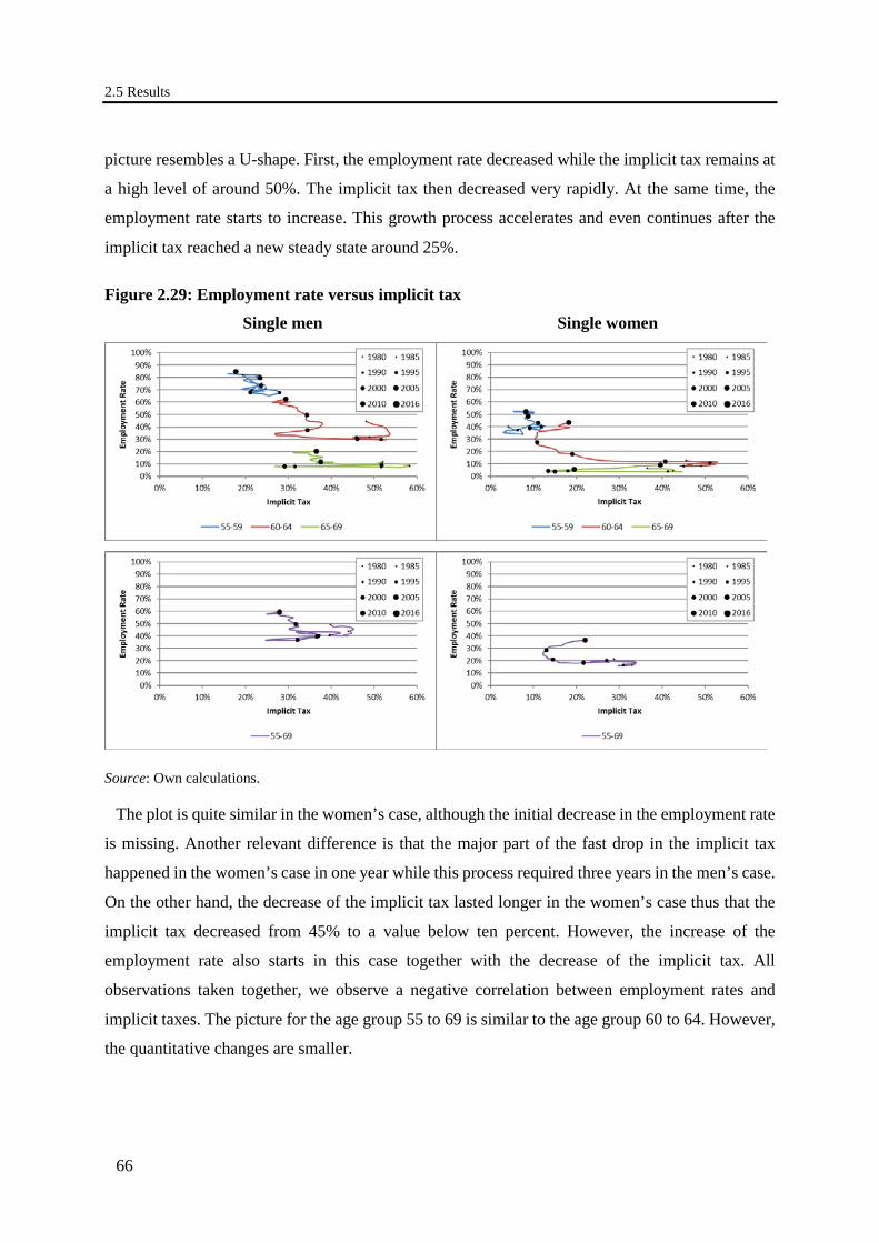
2.5 Results
66
picture resembles a U-shape. First, the employment rate decreased while the implicit tax remains at
a high level of around 50%. The implicit tax then decreased very rapidly. At the same time, the
employment rate starts to increase. This growth process accelerates and even continues after the
implicit tax reached a new steady state around 25%.
Figure 2.29: Employment rate versus implicit tax
Single men Single women
Source: Own calculations.
The plot is quite similar in the women’s case, although the initial decrease in the employment rate
is missing. Another relevant difference is that the major part of the fast drop in the implicit tax
happened in the women’s case in one year while this process required three years in the men’s case.
On the other hand, the decrease of the implicit tax lasted longer in the women’s case thus that the
implicit tax decreased from 45% to a value below ten percent. However, the increase of the
employment rate also starts in this case together with the decrease of the implicit tax. All
observations taken together, we observe a negative correlation between employment rates and
implicit taxes. The picture for the age group 55 to 69 is similar to the age group 60 to 64. However,
the quantitative changes are smaller.
2. Social Security Reforms and the Changing Retirement Behavior in Germany
67
2.5.7 Relation between implicit taxes and pension claiming ages
Finally, we compare the development of the implicit tax with the distribution of pension claiming
ages during the retirement window from 60 to 65. As mentioned before, we will consider hereby an
alternative weighting procedure such that the implicit taxes may differ slightly from those just
presented. However, the general development and the differences between the skill and age groups
do not change.
For the pension claiming behavior at a certain age a two implicit taxes are relevant. First, there is
the implicit tax of the previous age (a-1). If it becomes negative, it would indicate an incentive to
postpone the pension claiming by one year. Hence, one year later the number of individuals
claiming their pension at age a should increase. In fact, a decrease of the implicit tax at age (a-1)
could lead to an increase of the pension claiming as the monetary incentive to claim their pension
immediately declines. The other relevant implicit tax is the implicit tax of the current age. If the
implicit tax becomes smaller or even negative, postponing the pension entry becomes less
disadvantageous and can lead to a smaller share of pension claims at this age. Of course, there are
other factors like the abolishment of early retirement pathways which may counteract to the implicit
tax’s effect on the pension claiming behavior.
Figure 2.30 shows in separate graphs for each pension claiming age between 60 and 65 the
development of its share on all pension claims of the respective year (left side: men, right side:
women). Moreover, each graph includes the development of the implicit tax at the observed pension
claiming age and the previous year. In general, our observations are in line with the previous
discussions. We start with the pension claiming age 60. For both men and women, the implicit tax
of the previous age (59) does not change in a relevant way. Hence, there are no changes in the
incentive to leave the labor market at the age 59. On the other hand, there are quite large changes
in the implicit tax at the age of 60 as we have seen in the previous section. In line with our previous
argumentation these changes coincide with increases and decreases in the pension claims (i.e.,
higher (lower) implicit tax rates lead to more (fewer) pension claims). The decrease in pension
claims after the introduction of the actuarial deduction and their impact on the implicit taxes is
remarkable. Only the decrease in the pension claims after 2012 cannot be linked to a change in the
implicit tax. In fact, the reason for the drop is the abolishment of the old-age pension for women
and due to unemployment. Apparently, the abolishment of those pension pathways did not affect
the implicit taxes of the age 60 since both the social security wealth with an immediate and with a
postponed labor market exit are affected equally. For the pension claiming ages 61 and 62 the
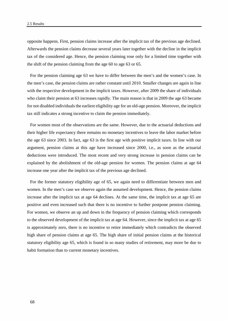
2.5 Results
68
opposite happens. First, pension claims increase after the implicit tax of the previous age declined.
Afterwards the pension claims decrease several years later together with the decline in the implicit
tax of the considered age. Hence, the pension claiming rose only for a limited time together with
the shift of the pension claiming from the age 60 to age 63 or 65.
For the pension claiming age 63 we have to differ between the men’s and the women’s case. In
the men’s case, the pension claims are rather constant until 2010. Smaller changes are again in line
with the respective development in the implicit taxes. However, after 2009 the share of individuals
who claim their pension at 63 increases rapidly. The main reason is that in 2009 the age 63 became
for not disabled individuals the earliest eligibility age for an old-age pension. Moreover, the implicit
tax still indicates a strong incentive to claim the pension immediately.
For women most of the observations are the same. However, due to the actuarial deductions and
their higher life expectancy there remains no monetary incentives to leave the labor market before
the age 63 since 2003. In fact, age 63 is the first age with positive implicit taxes. In line with our
argument, pension claims at this age have increased since 2000, i.e., as soon as the actuarial
deductions were introduced. The most recent and very strong increase in pension claims can be
explained by the abolishment of the old-age pension for women. The pension claims at age 64
increase one year after the implicit tax of the previous age declined.
For the former statutory eligibility age of 65, we again need to differentiate between men and
women. In the men’s case we observe again the assumed development. Hence, the pension claims
increase after the implicit tax at age 64 declines. At the same time, the implicit tax at age 65 are
positive and even increased such that there is no incentive to further postpone pension claiming.
For women, we observe an up and down in the frequency of pension claiming which corresponds
to the observed development of the implicit tax at age 64. However, since the implicit tax at age 65
is approximately zero, there is no incentive to retire immediately which contradicts the observed
high share of pension claims at age 65. The high share of initial pension claims at the historical
statutory eligibility age 65, which is found in so many studies of retirement, may more be due to
habit formation than to current monetary incentives.
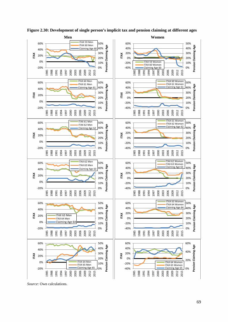
69
Figure 2.30: Development of single person’s implicit tax and pension claiming at different ages Men Women
Source: Own calculations.
0%10%20%30%40%50%
-20%
0%
20%
40%
60%19
8519
8819
9119
9419
9720
0020
0320
0620
0920
1220
15 Pens
ion
Clai
min
g Ag
e
ITAX
ITAX 59 MenITAX 60 MenClaiming Age 60
0%10%20%30%40%50%
-40%-20%
0%20%40%60%
1985
1988
1991
1994
1997
2000
2003
2006
2009
2012
2015 Pe
nsio
n Cl
aim
ing
Age
ITAX
ITAX 59 WomenITAX 60 WomenClaiming Age 60
0%
10%
20%
30%
40%
50%
-20%
0%
20%
40%
60%
1985
1988
1991
1994
1997
2000
2003
2006
2009
2012
2015 Pe
nsio
n Cl
aim
ing
Age
ITAX
ITAX 60 MenITAX 61 MenClaiming Age 61
0%
10%
20%
30%
40%
50%
-40%
-20%
0%
20%
40%
60%
1985
1988
1991
1994
1997
2000
2003
2006
2009
2012
2015 Pe
nsio
n Cl
aim
ing
Age
ITAX
ITAX 60 WomenITAX 61 WomenClaiming Age 61
0%
10%
20%
30%
40%
50%
-20%
0%
20%
40%
60%
1985
1988
1991
1994
1997
2000
2003
2006
2009
2012
2015 Pe
nsio
n Cl
aim
ing
Age
ITAX
ITAX 61 MenITAX 62 MenClaiming Age 62
0%
10%
20%
30%
40%
50%
-40%
-20%
0%
20%
40%
60%
1985
1988
1991
1994
1997
2000
2003
2006
2009
2012
2015 Pe
nsio
n Cl
aim
ing
Age
ITAX
ITAX 61 WomenITAX 62 WomenClaiming Age 62
0%
10%
20%
30%
40%
50%
-20%
0%
20%
40%
60%
1985
1988
1991
1994
1997
2000
2003
2006
2009
2012
2015 Pe
nsio
n Cl
aim
ing
Age
ITAX
ITAX 62 MenITAX 63 MenClaiming Age 63
0%
10%
20%
30%
40%
50%
-40%
-20%
0%
20%
40%
60%
1985
1988
1991
1994
1997
2000
2003
2006
2009
2012
2015 Pe
nsio
n Cl
aim
ing
Age
ITAX
ITAX 62 WomenITAX 63 WomenClaiming Age 63
0%
10%
20%
30%
40%
50%
-20%
0%
20%
40%
60%
1985
1988
1991
1994
1997
2000
2003
2006
2009
2012
2015 Pe
nsio
n Cl
aim
ing
Age
ITAX ITAX 63 Men
ITAX 64 MenClaiming Age 64
0%
10%
20%
30%
40%
50%
-40%
-20%
0%
20%
40%
60%
1985
1988
1991
1994
1997
2000
2003
2006
2009
2012
2015 Pe
nsio
n Cl
aim
ing
Age
ITAX
ITAX 63 WomenITAX 64 WomenClaiming Age 64
0%
10%
20%
30%
40%
50%
-20%
0%
20%
40%
60%
1985
1988
1991
1994
1997
2000
2003
2006
2009
2012
2015 Pe
nsio
n Cl
aim
ing
Age
ITAX
ITAX 64 MenITAX 65 MenClaiming Age 65 0%
20%
40%
60%
-40%
-20%
0%
20%
40%
60%
1985
1988
1991
1994
1997
2000
2003
2006
2009
2012
2015 Pe
nsio
n Cl
aim
ing
Age
ITAX
ITAX 64 WomenITAX 65 WomenClaiming Age 65
2.6 Conclusions
70
2.6 Conclusions
Employment of older individuals in Germany has experienced a remarkable reversal around the late
1990s. After a long declining trend that began in the early 1970s, the employment rate for older
men has strongly increased again. This increase has lasted until today. In contrast, employment of
older women in Germany has experienced a less pronounced U-shaped pattern in particular because
employment of younger women has steadily increased since the 1970s. This study has linked these
trends to changes in public pension policies. The key instrument of our analysis is the concept of
“implicit taxes on working longer” (ITAX) which represents the monetary incentives that
individuals face in their labor supply and pension claiming decisions. In this article, we compute
implicit taxes for a set of synthetic individuals differing by household demographics and
education/skill, once based on a common macro environment across all 12 countries part of the
International Social Security Project and once based on German age-earnings profiles, payroll taxes
and survival probabilities.
We find that for both men and women the increase in the employment rate coincides with a
reduction in the early retirement incentive expressed by the implicit taxes on working longer
(Figure 2.29). The reduction of incentives mainly stems from the introduction of actuarial
deductions for claiming a pension before the statutory eligibility age. In recent years, the
employment rate additionally increased due to the abolishment of early retirement pathways for
unemployed and women. We find similar correlations between the development of the implicit tax
and actual pension claiming behavior (Figure 2.30).
The evidence in Figure 2.29 and Figure 2.30 is highly suggestive. However, these bivariate
correlations of a relatively small set of synthetic individuals do not control for the many other
potential explanatory factors and the heterogeneity in the population. This requires a much more
elaborate multivariate analysis of actual individuals in panel data. The next step will therefore be
devoted to a causal analysis of the role of public pension policies in shaping old-age employment.
This is the objective of the following Chapter 3. We are doing this by constructing, for each
individual, time series of the implicit tax. We will then use these incentive variables, the macro
variables considered so far and other determinants on the individual level as explanatory variables
in an econometric analysis of retirement and labor force participation.
71
3. Retirement Decisions in Germany: Micro-Modelling
This chapter was written in co-authorship with Axel Börsch-Supan, Irene Ferrari and
Johannes Rausch.20
3.1 Introduction
Employment in older ages has declined for a long time in Germany, even for women, reaching a
level of only 36.8/21.5% (men/women) in 2000 for the 55-69 age group (see Figure 3.1). Since
about 2000, however, working later in life has been making a stark comeback. West Germany has
actually experienced the largest increase in the employment rate of the 55-69 age group in
comparison to the other countries part of the International Social Security Project (ISSP). In 2016,
the employment rate has reached a level of 59.5/48.6% (OECD 2018a). The trend reversal is
particularly pronounced among men, while the picture is a bit more complex for women who
experienced a rather constant increase for the 55-59 age group and a mild reversal for the other age
groups.
Understanding the causes for this recent increase in employment is important if one wants to
assess whether the current rising trend will continue, thus reducing the negative consequences of
aging on fiscal sustainability. If the reversal is mainly caused by transitory or one-off events, old-
age labor force participation may slow down again in the near future. However, if it is indeed caused
by a structural change, we may expect a lasting impact on fiscal sustainability.
20 This study uses data from German Socio-Economic Panel (GSOEP), data for years 1984-2016, version 33, SOEP, 2020, doi:10.5684/soep.v33, see Goebel et al. (2019).
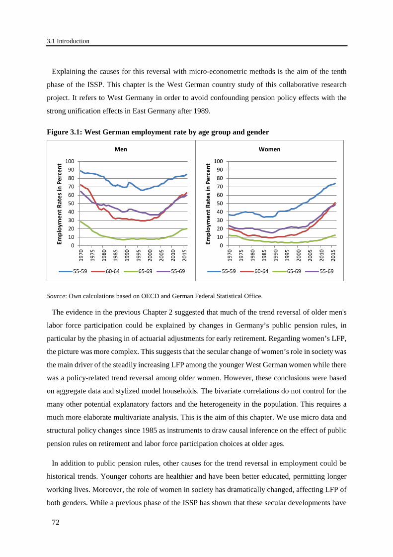
3.1 Introduction
72
Explaining the causes for this reversal with micro-econometric methods is the aim of the tenth
phase of the ISSP. This chapter is the West German country study of this collaborative research
project. It refers to West Germany in order to avoid confounding pension policy effects with the
strong unification effects in East Germany after 1989.
Figure 3.1: West German employment rate by age group and gender
Source: Own calculations based on OECD and German Federal Statistical Office.
The evidence in the previous Chapter 2 suggested that much of the trend reversal of older men's
labor force participation could be explained by changes in Germany’s public pension rules, in
particular by the phasing in of actuarial adjustments for early retirement. Regarding women’s LFP,
the picture was more complex. This suggests that the secular change of women’s role in society was
the main driver of the steadily increasing LFP among the younger West German women while there
was a policy-related trend reversal among older women. However, these conclusions were based
on aggregate data and stylized model households. The bivariate correlations do not control for the
many other potential explanatory factors and the heterogeneity in the population. This requires a
much more elaborate multivariate analysis. This is the aim of this chapter. We use micro data and
structural policy changes since 1985 as instruments to draw causal inference on the effect of public
pension rules on retirement and labor force participation choices at older ages.
In addition to public pension rules, other causes for the trend reversal in employment could be
historical trends. Younger cohorts are healthier and have been better educated, permitting longer
working lives. Moreover, the role of women in society has dramatically changed, affecting LFP of
both genders. While a previous phase of the ISSP has shown that these secular developments have
0102030405060708090
100
1970
1975
1980
1985
1990
1995
2000
2005
2010
2015
Empl
oym
ent R
ates
in P
erce
nt
Men
55-59 60-64 65-69 55-69
0102030405060708090
100
1970
1975
1980
1985
1990
1995
2000
2005
2010
2015
Empl
oym
ent R
ates
in P
erce
nt
Women
55-59 60-64 65-69 55-69
3. Retirement Decisions in Germany: Micro-Modelling
73
contributed astonishingly little to the trend reversal (Coile et al. 2019 for an overview; Börsch-
Supan and Ferrari 2019 for Germany), we use a set of covariates to account for these changes.
Overall, this study contributes to the large empirical literature studying individual retirement
responses to varying incentives in the old-age security system. The study is closely related to the
work that was done by Gruber and Wise (1999, 2004), who investigated the effect of retirement
incentives on the downturn of labor force participation of older individuals at the end of last century.
They found that retirement incentives had a strong effect on retirement decisions. More recent
empirical investigations have shown that specific reform devices have led to substantial reactions
of older individuals’ labor market behavior, albeit at varying magnitudes. Existing studies evaluated
specific reforms such as the introduction of actuarial adjustments for early retirement (Hanel 2010,
Engels et al. 2017, Giesecke 2018), the increase of the earliest eligibility age for early retirement
(Geyer and Welteke 2017 and Geyer et al. 2020), the reform that increased the generosity of a
specific early retirement pathway for individuals with at least 45 insurance years (Dolls and Krolage
2019), an earlier reform on supplemental pension benefits (Ye 2018), a reform on disability
insurance (Hanel 2012), and whether the 2006 unemployment insurance reform affected older
workers’ labor market transitions (Riphahn and Schrader 2019). Beside financial incentives,
Seibold (2019) found that reference point effects are a potential explanation of retirement patterns
as well.
The key novelty of this study lies in investigating the reform effect of structural policy changes
on retirement and employment choices at older ages over almost four decades. Within this
observation period, Germany experienced a considerable reversal of employment rates and several
reforms. However, limitations and questions for future research remain open. For instance, the
analyses in this study primarily focus on how structural policy changes have influenced labor market
behavior of the average older individual. However, the reforms may affect heterogeneous groups
of individuals differently, depending on, e.g, the individuals’ income situation, employment history
or health (see, e.g., Giesecke 2018). Future research on the heterogeneous effects of structural policy
changes can help to better understand the variety of reform effects.
The chapter is organized as follows. Section 3.2 provides a summary of the institutional changes
and pension reforms in Germany that may be the causes for the observed trend reversal. Sections 3.3
and 3.4 are the main methodological parts of the chapter and describe our data (Section 3.3) and
our main explanatory variable, the “implicit tax on working longer” (Section 3.4). Section 3.5
validates our pension calculator and Section 3.6 shows how we deal with expected pension benefits
3.2 German public pension system
74
for all labor market exit ages of our retirement window. Section 3.7 presents our regression results.
We then use these results to counterfactually predict what would have happened to labor force
participation if the pension rules underlying the implicit tax on working longer had not changed
since the 1980s (Section 3.8). Indeed, old-age labor force participation would have been
substantially lower than it is today. Section 2.9 therefore concludes, that the negative correlation
between the employment rate and the incentives to claim benefits early found in Chapter 2 has a
causal interpretation: as the implicit tax on working longer decreased, employment at older ages
increased.
3.2 German public pension system
In this section, we outline the German public pension system (Gesetzliche Rentenversicherung,
GRV) and its general aspects. We primarily focus on the properties and the main mechanics we
need for the analysis in this study. As this study is part of a multistage research project, a
comprehensive analysis of the institutional details, the reforms process in the past decades and the
resulting financial incentives for typical individuals has been carried out in the first step of this
research project (see Chapter 2 of this dissertation).
The German public pension system was the first formal pension system in the world. It goes back
to German Chancellor Otto von Bismarck, originally conceived as a funded disability insurance
scheme in 1889. In the beginning, “old age” was classified as a subcategory of disability. “Disability
benefits due to old age” were lower compared to real disability benefits and were granted starting
from age 70. With further reforms in the following years (in particular in 1899, 1911, 1913, 1916),
the scheme was broadened into a general old-age security system with disability pensions and mere
old-age pensions. Benefits of disability pensions and old-age pensions were set on the same level
and the coverage among workers and employees was increasingly enlarged. The eligibility age was
lowered to 65 for employees in 1913 and for workers in 1916 (DRV 2020). After two world wars
and a period of hyperinflation, about half of the capital stock was lost and the system was
transformed into a pay-as-you-go (PAYG) system in 1957, where the pensions of current retirees
are financed by the contributions of current workers.
The public pension system features a very broad coverage of workers. About 85% of the German
workforce are part of the system. For most of the insurants, pension entitlements from the public
pension system is the most important income source in old age. In fact, for the majority of the
insurants, public pension benefits were even the only source of income in old age until the end of

3. Retirement Decisions in Germany: Micro-Modelling
75
the 1990s. For this reason, the German public pension system was considered a monolithic pension
system. Caused by the decline in birth rates since the 1970s and a parallel increase in life
expectancy, demographic change has led to a paradigm shift at the end of the 1990s. With the 2001
pension reform the public old-age provision in Germany was transformed into a three-pillar system.
In the three-pillar system, public pension benefits are still regarded as main source of income in old
age (first pillar). However, in order to maintain their previous living standard, retirees are meant to
top up public pension benefits with occupational pension benefits (second pillar) and benefits from
private pensions (third pillar). Until today, first-pillar public pension benefits still shape the current
retirees’ income in old age. Second- and third-pillar benefits do play a minor role in providing old-
age income. For that reason, we focus on the public pension system in our analysis.
Coverage and contributions. The scheme is mandatory for all private and public employees and
covers about 85% of the German workforce. Civil servants, about 5%, are not part of the public
pension scheme and have their own old-age provision scheme. With the exception of certain groups,
the self-employed (roughly 10% of the workforce) also have their own pension systems.
Roughly 77% of the budget of the public pension scheme is financed by contributions of the
insurants. The contributions are administrated like a payroll tax, levied equally on employees and
employers. In 2018, the contribution rate was 18.6% on the first 78,000€ of yearly gross income.
The latter is the upper-earnings threshold (Beitragsbemessungsgrenze) and represents about the
double of the average yearly gross income of all insured individuals in the public pension system.21
Technically, contributions are split evenly between employees and employers. The remaining
approximately 23% of the public pension system budget is financed by governmental subsidies
(Bundeszuschüsse).
21 The values refer to West Germany only (see DRV 2018).
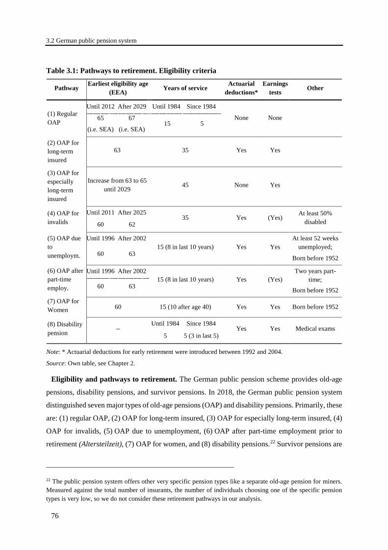
3.2 German public pension system
76
Table 3.1: Pathways to retirement. Eligibility criteria
Pathway Earliest eligibility age
(EEA) Years of service
Actuarial deductions*
Earnings tests
Other
(1) Regular OAP
Until 2012 After 2029 Until 1984 Since 1984
None None
65
(i.e. SEA)
67
(i.e. SEA) 15 5
(2) OAP for long-term insured
63 35 Yes Yes
(3) OAP for especially long-term insured
Increase from 63 to 65 until 2029
45 None Yes
(4) OAP for invalids
Until 2011 After 2025 35 Yes (Yes)
At least 50% disabled 60 62
(5) OAP due to unemploym.
Until 1996 After 2002 15 (8 in last 10 years) Yes Yes
At least 52 weeks unemployed;
Born before 1952 60 63
(6) OAP after part-time employ.
Until 1996 After 2002 15 (8 in last 10 years) Yes (Yes)
Two years part-time;
Born before 1952 60 63
(7) OAP for Women 60 15 (10 after age 40) Yes Yes Born before 1952
(8) Disability pension –
Until 1984 Since 1984 Yes Yes Medical exams
5 5 (3 in last 5)
Note: * Actuarial deductions for early retirement were introduced between 1992 and 2004.
Source: Own table, see Chapter 2.
Eligibility and pathways to retirement. The German public pension scheme provides old-age
pensions, disability pensions, and survivor pensions. In 2018, the German public pension system
distinguished seven major types of old-age pensions (OAP) and disability pensions. Primarily, these
are: (1) regular OAP, (2) OAP for long-term insured, (3) OAP for especially long-term insured, (4)
OAP for invalids, (5) OAP due to unemployment, (6) OAP after part-time employment prior to
retirement (Altersteilzeit), (7) OAP for women, and (8) disability pensions.22 Survivor pensions are
22 The public pension system offers other very specific pension types like a separate old-age pension for miners. Measured against the total number of insurants, the number of individuals choosing one of the specific pension types is very low, so we do not consider these retirement pathways in our analysis.
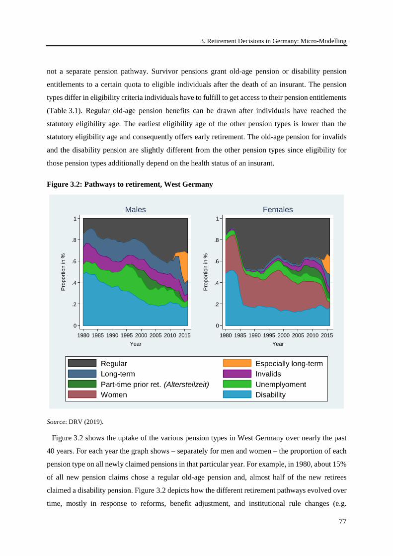
3. Retirement Decisions in Germany: Micro-Modelling
77
not a separate pension pathway. Survivor pensions grant old-age pension or disability pension
entitlements to a certain quota to eligible individuals after the death of an insurant. The pension
types differ in eligibility criteria individuals have to fulfill to get access to their pension entitlements
(Table 3.1). Regular old-age pension benefits can be drawn after individuals have reached the
statutory eligibility age. The earliest eligibility age of the other pension types is lower than the
statutory eligibility age and consequently offers early retirement. The old-age pension for invalids
and the disability pension are slightly different from the other pension types since eligibility for
those pension types additionally depend on the health status of an insurant.
Figure 3.2: Pathways to retirement, West Germany
Source: DRV (2019).
Figure 3.2 shows the uptake of the various pension types in West Germany over nearly the past
40 years. For each year the graph shows – separately for men and women – the proportion of each
pension type on all newly claimed pensions in that particular year. For example, in 1980, about 15%
of all new pension claims chose a regular old-age pension and, almost half of the new retirees
claimed a disability pension. Figure 3.2 depicts how the different retirement pathways evolved over
time, mostly in response to reforms, benefit adjustment, and institutional rule changes (e.g.
0
.2
.4
.6
.8
1
Prop
ortio
n in
%
1980 1985 1990 1995 2000 2005 2010 2015Year
Males
0
.2
.4
.6
.8
1
Prop
ortio
n in
%
1980 1985 1990 1995 2000 2005 2010 2015Year
Females
Regular Especially long-termLong-term InvalidsPart-time prior ret. (Altersteilzeit) UnemplyomentWomen Disability
3.2 German public pension system
78
tightening of the disability screening process, for details see Chapter 2). The figure shows the
multitude of possible retirement pathways. A major undertaking of this paper is to account for this
diversity.
Benefits and taxation. Pension benefits of the PAYG public pension system are related to the
individual earnings and contributions history. Pension benefits are computed according to the
pension benefit formula as the product of two individual components (1, 2) and two universal
components (3, 4): the individual components are (1) the sum of earnings points an individual has
accumulated over her working career (Entgeltpunkte) and (2) an access factor which captures
actuarial adjustments for early or late retirement (Zugangsfaktor). The universal components are
(3) the current pension value (aktueller Rentenwert) and a (4) pension type factor (Rentenartfaktor).
(1) The sum of earnings points represents the individual earnings history. The earnings points
ensure a relation between earnings and benefits (exceptions for care, unemployment, disability etc.).
Earnings points are calculated by dividing the individual gross income by the average income of all
insurants in the public pension system. If the individual’s earnings are exactly the average gross
earnings of all insurants, then this individual receives one earnings point. Half the average gross
income entails 0.5 earnings points, etc. The official government computations, such as the official
replacement rate (Rentenniveau), are based on a pensioner with forty-five contributions years and
average earnings in each year. This standardized pensioner (Eckrentner) accumulates exactly forty-
five earnings points. (2) The access factor (Zugangsfaktor) captures actuarial adjustments for early
or late retirement. Actuarial deductions apply if individuals claim pension benefits before the
statutory eligibility age. For each year of early retirement, pension benefits are reduced by 3.6%. In
the 1992 pension reform, actuarial supplements for late retirement were adjusted. Late retirement
is the practice of postponing benefit claiming beyond the SEA. For each year of late retirement,
actuarial supplements of 6% are granted for postponing the pension claiming beyond the statutory
eligibility age.23 The factor equals one if individuals claim pension benefits at the statutory
eligibility age or a pension-type-specific full rate age where no adjustments apply (e.g. age 63 for
individuals born until 1952 with forty-five service years). (3) The current pension value indicates
the relationship between average earnings and pension benefits. The current pension value is the
amount of monthly pension benefits related to one earnings point.24 Each year, the current pension
23 Actuarial supplements were already introduced in 1972. Until the 1992 reform, however, only for two years of late retirement actuarial supplements in the amount of 7.2% applied (i.e. until age 66 and 67). 24 Note that the pension benefit calculation is the base in the computation of social security wealth in Section 3.4.
3. Retirement Decisions in Germany: Micro-Modelling
79
value is replaced with a new value by law. (4) The pension type factor (Rentenartfaktor) reflects
the type of pension and the percentage of pension entitlements. The pension type factor is for
example one for old-age pensions and full disability pension benefits, and 0.55 (0.6 until 2001) for
full survivor benefits (große Witwen-/Witwerrente).
Until 2004, pension benefits were only taxed if benefits surpassed a quite large allowance. This
affected only relatively few cases. With the 2004 pension reform coming into effect in 2005,
deferred taxation of pension was introduced. Thus, contributions to the public pension system
became tax exempted and the pension benefits taxable. To prevent a double taxation the reform
included a generous transition period until 2040.
3.3 Data and variable specification
In the following sections, we will introduce our main data source, the German Socio-Economic
Panel (GSOEP), and we will describe our strategy for constructing the income profiles using the
panel data. We will then explain how we define retirement status – our outcome variable – and how
we handle the choice of multiple retirement pathways. Finally, we will check our pension
calculations against the actual pension received by individuals, as reported in GSOEP.
3.3.1 The German Socio-Economic Panel
The German Socio-Economic Panel (GSOEP) is a representative longitudinal study of private
households (see Goebel et al. 2019). Interviews take place annually and the sample size has
currently reached around 30,000 respondents in around 11,000 households. GSOEP was started in
1984 and we include waves up to 2015, therefore we can count on 32 consecutive years of data.
This is particularly convenient for the current analysis, as this time span includes the reversal of
older men’s labor force participation since around the late 1990s. Furthermore, several pension
reforms were implemented during these years which provide variation in pension incentives
necessary for the identification of our retirement model.
GSOEP includes several subsamples, each with different sampling probabilities that were chosen
to ensure that the number of cases are large enough for separate analyses of each sample.25 We draw
25 The subsamples consist, among others, of West German citizens, East German citizens, immigrants, high income individuals, as well as several refreshment samples.

3.3 Data and variable specification
80
our sample from the sample of West German citizens, as retirement patterns in East Germany are
affected by the transition to a market economy and slightly different pension rules.
The data provide information on all household members and contain a stable set of core
demographic and economic questions, including labor market status, gross and net income, hours
worked, education and marital status. Since each member in the household is interviewed, we have
the same information for both spouses.
A further advantage of the dataset is the possibility of constructing individuals’ labor history since
the age of 15. Individuals are asked once to provide information on their activity status over their
entire life course up to the time of the interview. The information provided is in the form of spells
of activities and distinguishes between time spent in education, doing apprenticeship or training, in
the military force or community service, in full-time employment, in part-time employment,
unemployed, out of the labor force or pensioner.
This retrospective occupation history can be integrated with information on the activity status
during the sample period, as GSOEP also collects detailed information on occupation in the form
of a calendar, with monthly information on labor market status.
On the other hand, while information on labor income is available for the sample period, no
retrospective information is available. Furthermore, the dataset includes little or irregular
information on health – especially objective measures of heath – and on household wealth.
Our sample selection is mostly based on two criteria. The first one is age: we keep individuals
aged 55 or above until retirement, or until age 70 if they are not yet retired by this age. Second, we
only keep employees of the private and public sector, therefore excluding civil servants and self-
employed workers, as participation in the public pension system is not mandatory for these two
latter categories of workers. This leaves us with around 5,000 individuals and 21,000 panel-year
observations, with an average and median observation time equal to 4.2 and four years, respectively.
In Table 3.2, we show some descriptive statistics of the main variables in our sample.
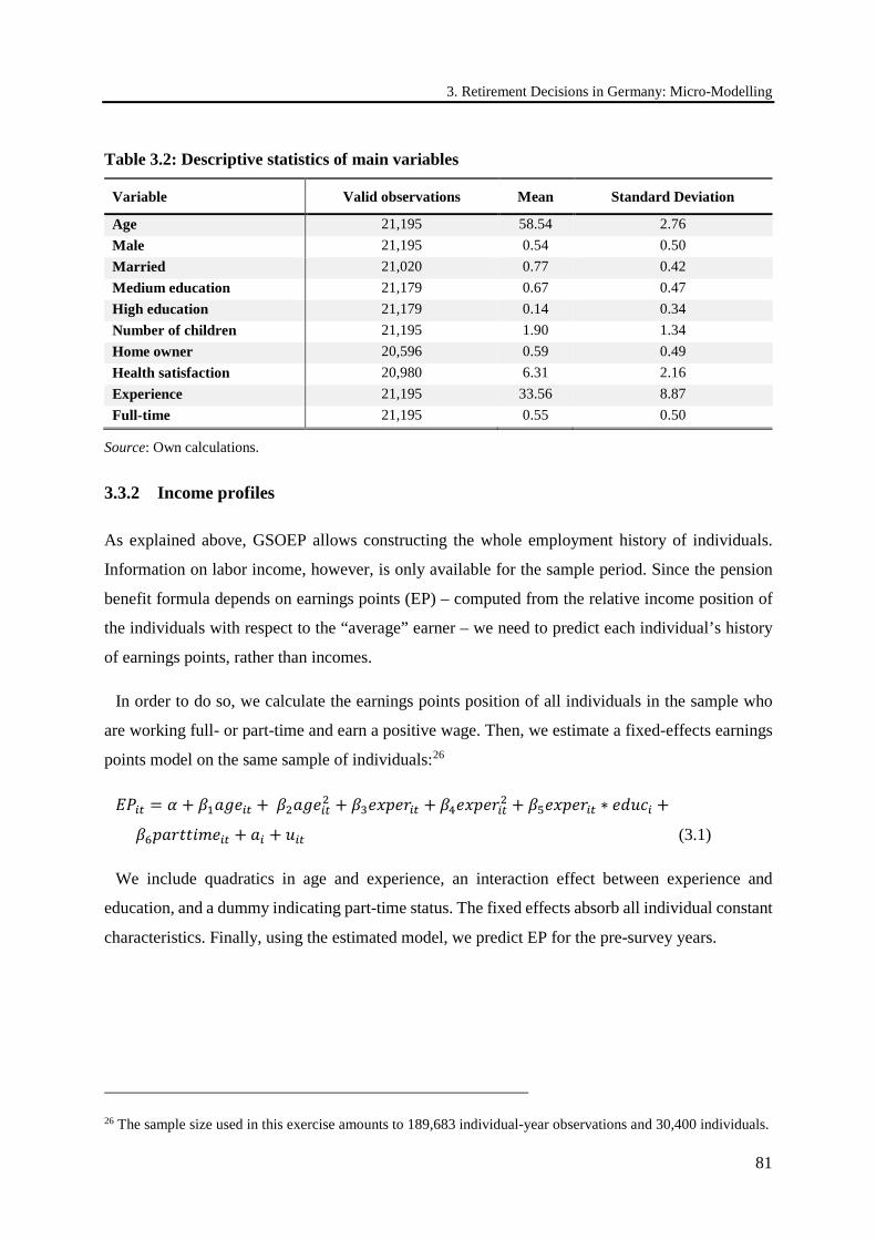
3. Retirement Decisions in Germany: Micro-Modelling
81
Table 3.2: Descriptive statistics of main variables
Variable Valid observations Mean Standard Deviation
Age 21,195 58.54 2.76 Male 21,195 0.54 0.50 Married 21,020 0.77 0.42 Medium education 21,179 0.67 0.47 High education 21,179 0.14 0.34 Number of children 21,195 1.90 1.34 Home owner 20,596 0.59 0.49 Health satisfaction 20,980 6.31 2.16 Experience 21,195 33.56 8.87 Full-time 21,195 0.55 0.50
Source: Own calculations.
3.3.2 Income profiles
As explained above, GSOEP allows constructing the whole employment history of individuals.
Information on labor income, however, is only available for the sample period. Since the pension
benefit formula depends on earnings points (EP) – computed from the relative income position of
the individuals with respect to the “average” earner – we need to predict each individual’s history
of earnings points, rather than incomes.
In order to do so, we calculate the earnings points position of all individuals in the sample who
are working full- or part-time and earn a positive wage. Then, we estimate a fixed-effects earnings
points model on the same sample of individuals:26
𝐸𝐸𝐸𝐸𝑖𝑖𝑡𝑡 = 𝛼𝛼 + 𝛽𝛽1𝑎𝑎𝑎𝑎𝑎𝑎𝑖𝑖𝑡𝑡 + 𝛽𝛽2𝑎𝑎𝑎𝑎𝑎𝑎𝑖𝑖𝑡𝑡2 + 𝛽𝛽3𝑎𝑎𝑒𝑒𝑒𝑒𝑎𝑎𝑟𝑟𝑖𝑖𝑡𝑡 + 𝛽𝛽4𝑎𝑎𝑒𝑒𝑒𝑒𝑎𝑎𝑟𝑟𝑖𝑖𝑡𝑡2 + 𝛽𝛽5𝑎𝑎𝑒𝑒𝑒𝑒𝑎𝑎𝑟𝑟𝑖𝑖𝑡𝑡 ∗ 𝑎𝑎𝑒𝑒𝑒𝑒𝑐𝑐𝑖𝑖 +
𝛽𝛽6𝑒𝑒𝑎𝑎𝑟𝑟𝑝𝑝𝑝𝑝𝑖𝑖𝑝𝑝𝑎𝑎𝑖𝑖𝑡𝑡 + 𝑎𝑎𝑖𝑖 + 𝑒𝑒𝑖𝑖𝑡𝑡 (3.1)
We include quadratics in age and experience, an interaction effect between experience and
education, and a dummy indicating part-time status. The fixed effects absorb all individual constant
characteristics. Finally, using the estimated model, we predict EP for the pre-survey years.
26 The sample size used in this exercise amounts to 189,683 individual-year observations and 30,400 individuals.
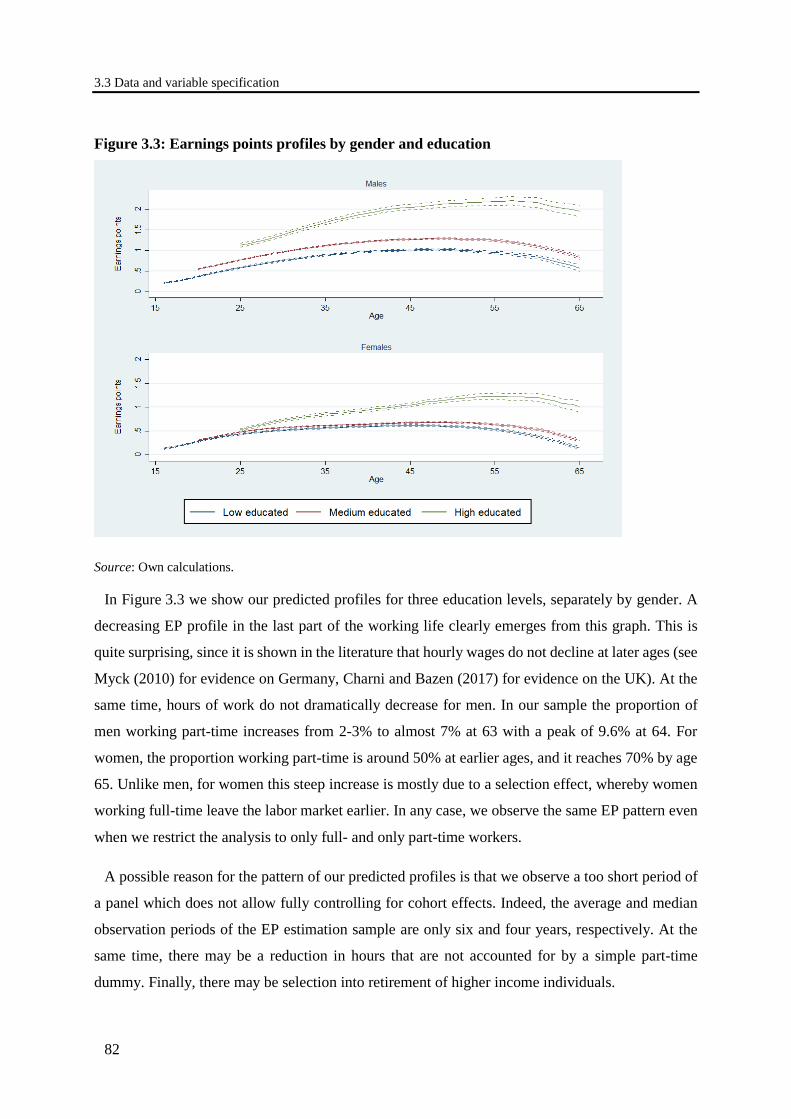
3.3 Data and variable specification
82
Figure 3.3: Earnings points profiles by gender and education
Source: Own calculations.
In Figure 3.3 we show our predicted profiles for three education levels, separately by gender. A
decreasing EP profile in the last part of the working life clearly emerges from this graph. This is
quite surprising, since it is shown in the literature that hourly wages do not decline at later ages (see
Myck (2010) for evidence on Germany, Charni and Bazen (2017) for evidence on the UK). At the
same time, hours of work do not dramatically decrease for men. In our sample the proportion of
men working part-time increases from 2-3% to almost 7% at 63 with a peak of 9.6% at 64. For
women, the proportion working part-time is around 50% at earlier ages, and it reaches 70% by age
65. Unlike men, for women this steep increase is mostly due to a selection effect, whereby women
working full-time leave the labor market earlier. In any case, we observe the same EP pattern even
when we restrict the analysis to only full- and only part-time workers.
A possible reason for the pattern of our predicted profiles is that we observe a too short period of
a panel which does not allow fully controlling for cohort effects. Indeed, the average and median
observation periods of the EP estimation sample are only six and four years, respectively. At the
same time, there may be a reduction in hours that are not accounted for by a simple part-time
dummy. Finally, there may be selection into retirement of higher income individuals.
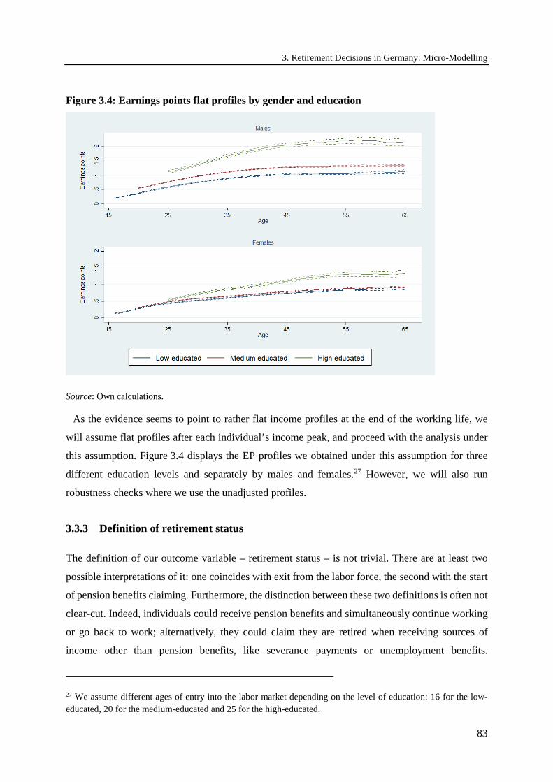
3. Retirement Decisions in Germany: Micro-Modelling
83
Figure 3.4: Earnings points flat profiles by gender and education
Source: Own calculations.
As the evidence seems to point to rather flat income profiles at the end of the working life, we
will assume flat profiles after each individual’s income peak, and proceed with the analysis under
this assumption. Figure 3.4 displays the EP profiles we obtained under this assumption for three
different education levels and separately by males and females.27 However, we will also run
robustness checks where we use the unadjusted profiles.
3.3.3 Definition of retirement status
The definition of our outcome variable – retirement status – is not trivial. There are at least two
possible interpretations of it: one coincides with exit from the labor force, the second with the start
of pension benefits claiming. Furthermore, the distinction between these two definitions is often not
clear-cut. Indeed, individuals could receive pension benefits and simultaneously continue working
or go back to work; alternatively, they could claim they are retired when receiving sources of
income other than pension benefits, like severance payments or unemployment benefits.
27 We assume different ages of entry into the labor market depending on the level of education: 16 for the low-educated, 20 for the medium-educated and 25 for the high-educated.
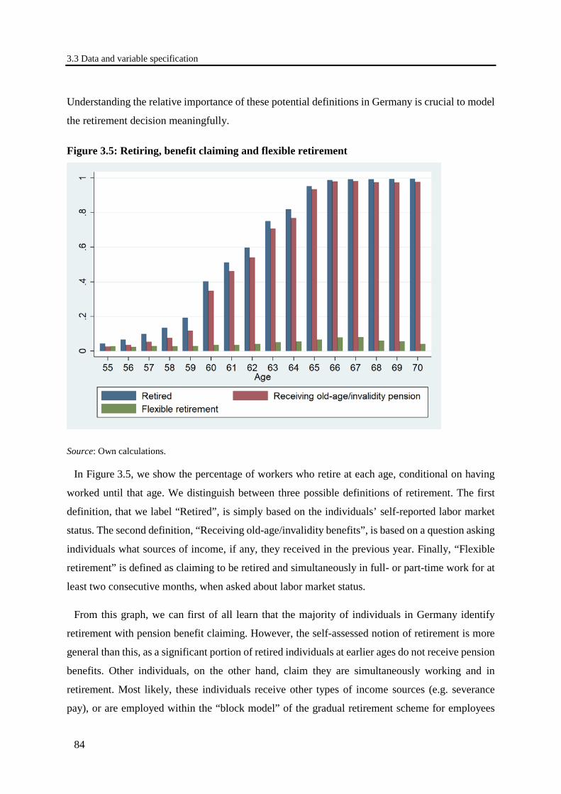
3.3 Data and variable specification
84
Understanding the relative importance of these potential definitions in Germany is crucial to model
the retirement decision meaningfully.
Figure 3.5: Retiring, benefit claiming and flexible retirement
Source: Own calculations.
In Figure 3.5, we show the percentage of workers who retire at each age, conditional on having
worked until that age. We distinguish between three possible definitions of retirement. The first
definition, that we label “Retired”, is simply based on the individuals’ self-reported labor market
status. The second definition, “Receiving old-age/invalidity benefits”, is based on a question asking
individuals what sources of income, if any, they received in the previous year. Finally, “Flexible
retirement” is defined as claiming to be retired and simultaneously in full- or part-time work for at
least two consecutive months, when asked about labor market status.
From this graph, we can first of all learn that the majority of individuals in Germany identify
retirement with pension benefit claiming. However, the self-assessed notion of retirement is more
general than this, as a significant portion of retired individuals at earlier ages do not receive pension
benefits. Other individuals, on the other hand, claim they are simultaneously working and in
retirement. Most likely, these individuals receive other types of income sources (e.g. severance
pay), or are employed within the “block model” of the gradual retirement scheme for employees
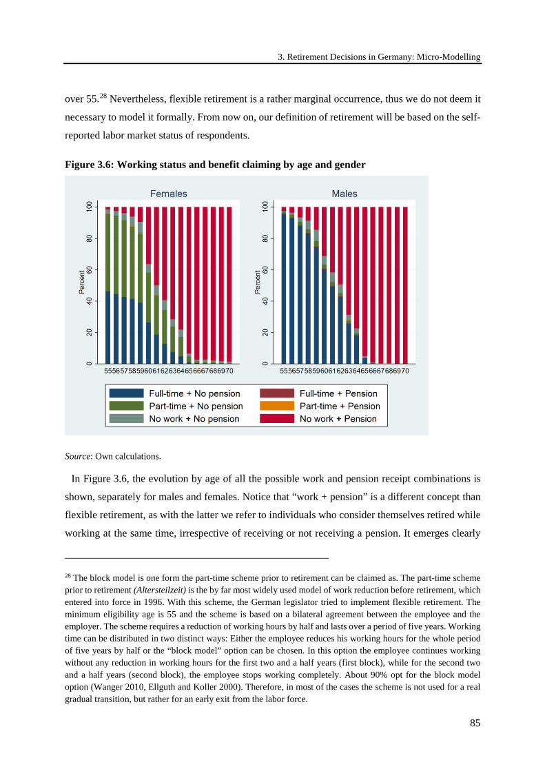
3. Retirement Decisions in Germany: Micro-Modelling
85
over 55.28 Nevertheless, flexible retirement is a rather marginal occurrence, thus we do not deem it
necessary to model it formally. From now on, our definition of retirement will be based on the self-
reported labor market status of respondents.
Figure 3.6: Working status and benefit claiming by age and gender
Source: Own calculations.
In Figure 3.6, the evolution by age of all the possible work and pension receipt combinations is
shown, separately for males and females. Notice that “work + pension” is a different concept than
flexible retirement, as with the latter we refer to individuals who consider themselves retired while
working at the same time, irrespective of receiving or not receiving a pension. It emerges clearly
28 The block model is one form the part-time scheme prior to retirement can be claimed as. The part-time scheme prior to retirement (Altersteilzeit) is the by far most widely used model of work reduction before retirement, which entered into force in 1996. With this scheme, the German legislator tried to implement flexible retirement. The minimum eligibility age is 55 and the scheme is based on a bilateral agreement between the employee and the employer. The scheme requires a reduction of working hours by half and lasts over a period of five years. Working time can be distributed in two distinct ways: Either the employee reduces his working hours for the whole period of five years by half or the “block model” option can be chosen. In this option the employee continues working without any reduction in working hours for the first two and a half years (first block), while for the second two and a half years (second block), the employee stops working completely. About 90% opt for the block model option (Wanger 2010, Ellguth and Koller 2000). Therefore, in most of the cases the scheme is not used for a real gradual transition, but rather for an early exit from the labor force.
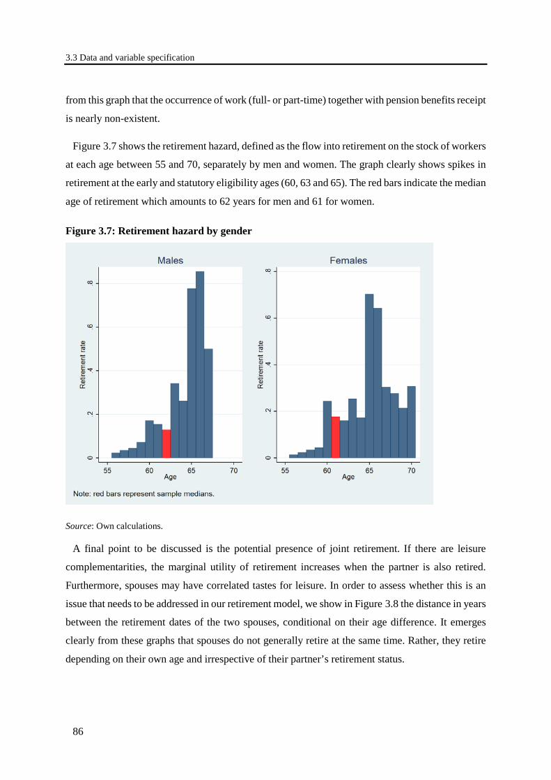
3.3 Data and variable specification
86
from this graph that the occurrence of work (full- or part-time) together with pension benefits receipt
is nearly non-existent.
Figure 3.7 shows the retirement hazard, defined as the flow into retirement on the stock of workers
at each age between 55 and 70, separately by men and women. The graph clearly shows spikes in
retirement at the early and statutory eligibility ages (60, 63 and 65). The red bars indicate the median
age of retirement which amounts to 62 years for men and 61 for women.
Figure 3.7: Retirement hazard by gender
Source: Own calculations.
A final point to be discussed is the potential presence of joint retirement. If there are leisure
complementarities, the marginal utility of retirement increases when the partner is also retired.
Furthermore, spouses may have correlated tastes for leisure. In order to assess whether this is an
issue that needs to be addressed in our retirement model, we show in Figure 3.8 the distance in years
between the retirement dates of the two spouses, conditional on their age difference. It emerges
clearly from these graphs that spouses do not generally retire at the same time. Rather, they retire
depending on their own age and irrespective of their partner’s retirement status.
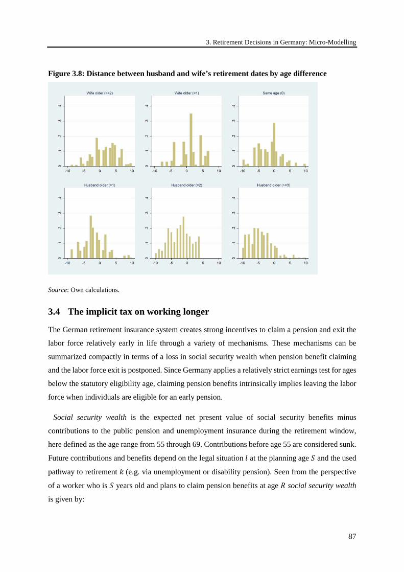
3. Retirement Decisions in Germany: Micro-Modelling
87
Figure 3.8: Distance between husband and wife’s retirement dates by age difference
Source: Own calculations.
3.4 The implicit tax on working longer
The German retirement insurance system creates strong incentives to claim a pension and exit the
labor force relatively early in life through a variety of mechanisms. These mechanisms can be
summarized compactly in terms of a loss in social security wealth when pension benefit claiming
and the labor force exit is postponed. Since Germany applies a relatively strict earnings test for ages
below the statutory eligibility age, claiming pension benefits intrinsically implies leaving the labor
force when individuals are eligible for an early pension.
Social security wealth is the expected net present value of social security benefits minus
contributions to the public pension and unemployment insurance during the retirement window,
here defined as the age range from 55 through 69. Contributions before age 55 are considered sunk.
Future contributions and benefits depend on the legal situation 𝑙𝑙 at the planning age 𝑆𝑆 and the used
pathway to retirement 𝑘𝑘 (e.g. via unemployment or disability pension). Seen from the perspective
of a worker who is 𝑆𝑆 years old and plans to claim pension benefits at age 𝑅𝑅 social security wealth
is given by:
3.4 The implicit tax on working longer
88
𝑆𝑆𝑆𝑆𝑊𝑊𝑆𝑆,𝑘𝑘,𝑙𝑙(𝑅𝑅, 𝑖𝑖) = ∑ 𝐵𝐵𝑡𝑡,𝑘𝑘,𝑙𝑙(𝑅𝑅, 𝑖𝑖) ∙ 𝜎𝜎(𝑖𝑖)𝑆𝑆,𝑡𝑡 ∙ 𝛽𝛽𝑡𝑡−𝑆𝑆𝑇𝑇𝑡𝑡=𝑅𝑅 − ∑ 𝑐𝑐𝑡𝑡,𝑙𝑙 ∙ 𝑌𝑌𝑡𝑡(𝑖𝑖) ∙ σ(i)𝑆𝑆,𝑡𝑡 ∙ 𝛽𝛽𝑡𝑡−𝑆𝑆𝑅𝑅−1
𝑡𝑡=𝑆𝑆 (3.2)
with
𝑆𝑆𝑆𝑆𝑊𝑊: net present discounted value of retirement/unemployment benefits 𝑆𝑆: planning age 𝑅𝑅: benefit claiming age 𝑖𝑖: gender and skill type 𝑘𝑘: pathway to retirement 𝑙𝑙: legal situation at planning age 𝑆𝑆 𝑌𝑌𝑡𝑡(𝑖𝑖): gross labor income at age 𝑝𝑝 𝐵𝐵𝑡𝑡,𝑘𝑘,𝑙𝑙(𝑅𝑅, 𝑖𝑖): net benefits from pathway 𝑘𝑘 at age 𝑝𝑝 for benefit claiming age 𝑅𝑅 and legal situation 𝑙𝑙 𝑐𝑐𝑡𝑡,𝑙𝑙: contribution rate to pension and unemployment system at age 𝑝𝑝 for legal situation 𝑙𝑙 𝜎𝜎(𝑖𝑖)𝑆𝑆,𝑡𝑡: probability to survive at least until age t given survival until age 𝑆𝑆 𝛽𝛽: discount factor 𝛿𝛿 = 1/(1 + 𝑟𝑟). We choose the usual discount rate 𝑟𝑟 of 3%.
Postponing claiming social security benefits by one year has two effects on social security wealth.
On the one hand, the individual receives one year less of benefits which decreases social security
wealth. On the other hand, annual benefits increase with later claiming in most countries due to
additional contributions and actuarial adjustments. Additional contributions accrue because the
individual now works a year longer, and having an extra year of earnings included in the benefit
computation may result in an overall higher benefit amount. Moreover, in Germany as in almost all
other countries, benefits are adjusted upwardly if benefits are taken later than the statutory eligibility
age through the actuarial supplements. The balance between these mechanisms determines whether
social security wealth increases or decreases with earlier or later retirement.
The incentives to leave the labor market and claim pension benefits can be expressed by the
implicit tax on working longer which is based on the accrual of social security wealth. The accrual
is defined as the numerical increase or decrease of social security wealth by postponing the labor
market exit by one year. The implicit tax (𝐼𝐼𝐼𝐼𝐼𝐼𝐼𝐼) is the negative accrual of social security wealth
(𝐼𝐼𝐴𝐴𝐴𝐴) divided by the after tax earnings (𝑌𝑌𝑁𝑁𝑁𝑁𝑡𝑡) during the additional year of work:
𝐼𝐼𝐼𝐼𝐼𝐼𝐼𝐼 = − 𝐴𝐴𝐴𝐴𝐴𝐴𝑌𝑌𝑁𝑁𝑁𝑁𝑁𝑁
(3.3)
As long as the implicit tax is negative, it is rational to postpone the withdrawal from the labor
market unless labor/leisure preferences or similar considerations dominate the expected gain in
social security wealth. Negative implicit taxes from a certain age on are sufficient (although not
necessary) for leaving the labor market and claiming a pension at that age. A positive value of 𝐼𝐼𝐼𝐼𝐼𝐼𝐼𝐼,
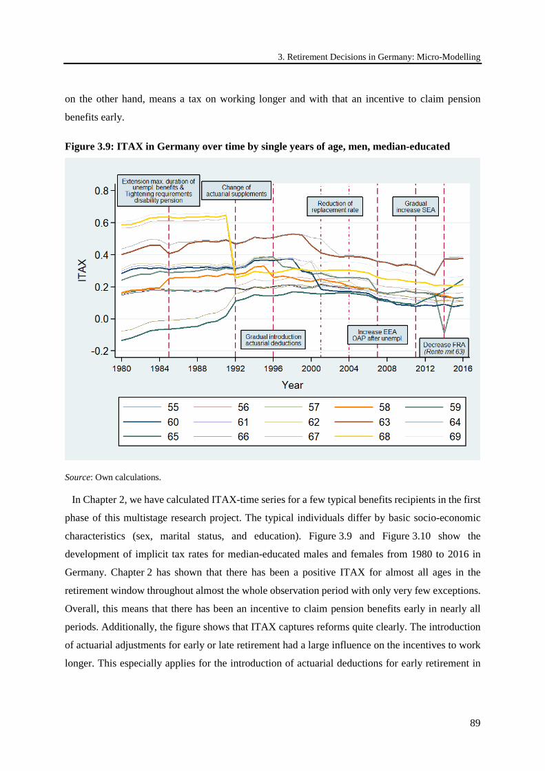
3. Retirement Decisions in Germany: Micro-Modelling
89
on the other hand, means a tax on working longer and with that an incentive to claim pension
benefits early.
Figure 3.9: ITAX in Germany over time by single years of age, men, median-educated
Source: Own calculations.
In Chapter 2, we have calculated ITAX-time series for a few typical benefits recipients in the first
phase of this multistage research project. The typical individuals differ by basic socio-economic
characteristics (sex, marital status, and education). Figure 3.9 and Figure 3.10 show the
development of implicit tax rates for median-educated males and females from 1980 to 2016 in
Germany. Chapter 2 has shown that there has been a positive ITAX for almost all ages in the
retirement window throughout almost the whole observation period with only very few exceptions.
Overall, this means that there has been an incentive to claim pension benefits early in nearly all
periods. Additionally, the figure shows that ITAX captures reforms quite clearly. The introduction
of actuarial adjustments for early or late retirement had a large influence on the incentives to work
longer. This especially applies for the introduction of actuarial deductions for early retirement in
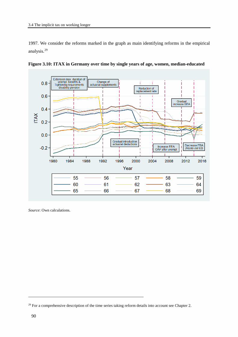
3.4 The implicit tax on working longer
90
1997. We consider the reforms marked in the graph as main identifying reforms in the empirical
analysis.29
Figure 3.10: ITAX in Germany over time by single years of age, women, median-educated
Source: Own calculations.
29 For a comprehensive description of the time series taking reform details into account see Chapter 2.
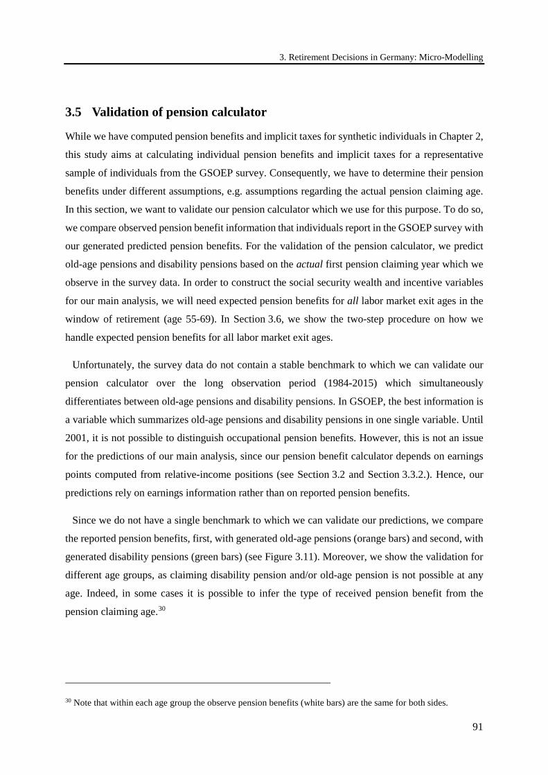
3. Retirement Decisions in Germany: Micro-Modelling
91
3.5 Validation of pension calculator
While we have computed pension benefits and implicit taxes for synthetic individuals in Chapter 2,
this study aims at calculating individual pension benefits and implicit taxes for a representative
sample of individuals from the GSOEP survey. Consequently, we have to determine their pension
benefits under different assumptions, e.g. assumptions regarding the actual pension claiming age.
In this section, we want to validate our pension calculator which we use for this purpose. To do so,
we compare observed pension benefit information that individuals report in the GSOEP survey with
our generated predicted pension benefits. For the validation of the pension calculator, we predict
old-age pensions and disability pensions based on the actual first pension claiming year which we
observe in the survey data. In order to construct the social security wealth and incentive variables
for our main analysis, we will need expected pension benefits for all labor market exit ages in the
window of retirement (age 55-69). In Section 3.6, we show the two-step procedure on how we
handle expected pension benefits for all labor market exit ages.
Unfortunately, the survey data do not contain a stable benchmark to which we can validate our
pension calculator over the long observation period (1984-2015) which simultaneously
differentiates between old-age pensions and disability pensions. In GSOEP, the best information is
a variable which summarizes old-age pensions and disability pensions in one single variable. Until
2001, it is not possible to distinguish occupational pension benefits. However, this is not an issue
for the predictions of our main analysis, since our pension benefit calculator depends on earnings
points computed from relative-income positions (see Section 3.2 and Section 3.3.2.). Hence, our
predictions rely on earnings information rather than on reported pension benefits.
Since we do not have a single benchmark to which we can validate our predictions, we compare
the reported pension benefits, first, with generated old-age pensions (orange bars) and second, with
generated disability pensions (green bars) (see Figure 3.11). Moreover, we show the validation for
different age groups, as claiming disability pension and/or old-age pension is not possible at any
age. Indeed, in some cases it is possible to infer the type of received pension benefit from the
pension claiming age.30
30 Note that within each age group the observe pension benefits (white bars) are the same for both sides.
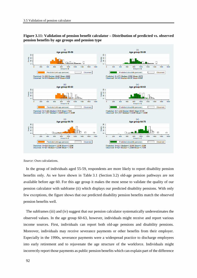
3.5 Validation of pension calculator
92
Figure 3.11: Validation of pension benefit calculator – Distribution of predicted vs. observed pension benefits by age groups and pension type
Source: Own calculations.
In the group of individuals aged 55-59, respondents are more likely to report disability pension
benefits only. As we have shown in Table 3.1 (Section 3.2) old-age pension pathways are not
available before age 60. For this age group it makes the most sense to validate the quality of our
pension calculator with subframe (ii) which displays our predicted disability pensions. With only
few exceptions, the figure shows that our predicted disability pension benefits match the observed
pension benefits well.
The subframes (iii) and (iv) suggest that our pension calculator systematically underestimates the
observed values. In the age group 60-63, however, individuals might receive and report various
income sources. First, individuals can report both old-age pensions and disability pensions.
Moreover, individuals may receive severance payments or other benefits from their employer.
Especially in the 1990s, severance payments were a widespread practice to discharge employees
into early retirement and to rejuvenate the age structure of the workforce. Individuals might
incorrectly report those payments as public pension benefits which can explain part of the difference
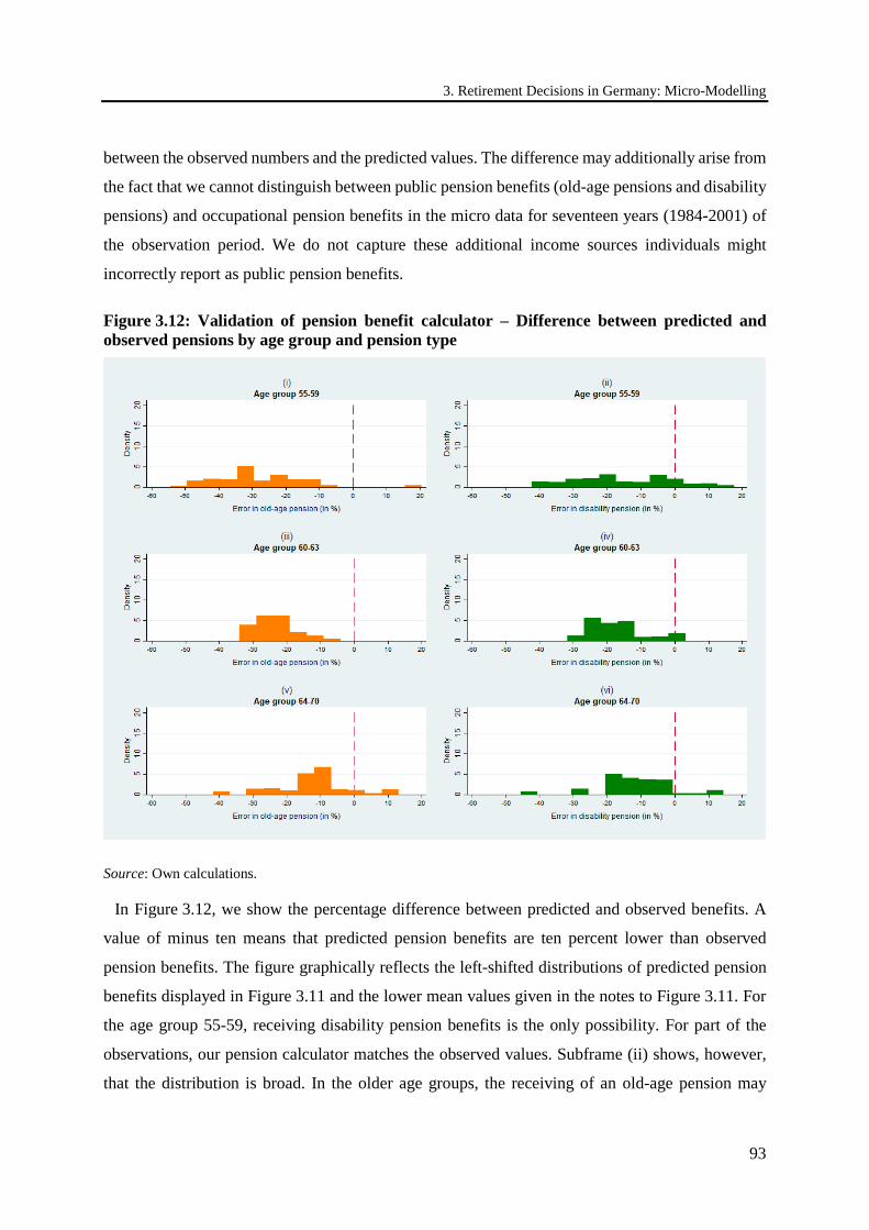
3. Retirement Decisions in Germany: Micro-Modelling
93
between the observed numbers and the predicted values. The difference may additionally arise from
the fact that we cannot distinguish between public pension benefits (old-age pensions and disability
pensions) and occupational pension benefits in the micro data for seventeen years (1984-2001) of
the observation period. We do not capture these additional income sources individuals might
incorrectly report as public pension benefits.
Figure 3.12: Validation of pension benefit calculator – Difference between predicted and observed pensions by age group and pension type
Source: Own calculations.
In Figure 3.12, we show the percentage difference between predicted and observed benefits. A
value of minus ten means that predicted pension benefits are ten percent lower than observed
pension benefits. The figure graphically reflects the left-shifted distributions of predicted pension
benefits displayed in Figure 3.11 and the lower mean values given in the notes to Figure 3.11. For
the age group 55-59, receiving disability pension benefits is the only possibility. For part of the
observations, our pension calculator matches the observed values. Subframe (ii) shows, however,
that the distribution is broad. In the older age groups, the receiving of an old-age pension may
3.6 Expected pension benefits on multiple pathways to retirement
94
coincide with receiving occupational pension benefits and other payments which we do not include
in our pension calculator (subframes iii and v).
Overall, our predicted pension benefits seem to underestimate the observed pensions. However,
the differences can most likely be explained with the receipt of occupational pension benefits and
other payments our pension calculator does not consider. However, since we focus on the evaluation
of incentives from the public pension system, our pension calculator seems to work reasonably well.
3.6 Expected pension benefits on multiple pathways to retirement
So far, we validated our pension calculator for individuals at their actual first pension claiming year.
For the construction of social security wealth and the incentive variables (see Section 3.4), we need
expected pension benefits for all labor market exit ages of our retirement window. At least
theoretically, there are several retirement pathways for a worker to exit the labor market and start
drawing from their public pension. The most important ones are:
• Regular old-age pension (at the statutory eligibility age), • Early pension claiming via old-age pension for (especially) long-term insured or for women, • Leaving the labor market via unemployment, • Part-time employment prior to retirement, • Early pension claiming via old-age pension for the disabled, and • Disability pension
It is important to notice that all of these pathways pay the same benefit once a person is eligible.
The main differences lie in the income between the labor market exit and first pension drawing.
However, in practice there is no free choice, as all of these pathways are subject to eligibility criteria
(see Table 3.1). Among those criteria, “strict” and “soft” eligibility rules can be distinguished. The
first are tied to objective variables, such as age, gender, and previous contribution history while the
second are subject to discretionary decisions, notably the determination of a workers’ disability
status.
We compute the expected pension benefits, which depend on the choice of the specific pathway,
in two steps. First, we compute the pension benefits for each pathway taking into account the “strict”
eligibility criteria only. Once an individual fulfills the criteria of a pathway this individual is
assumed to claim the pension as soon as possible. For example, a 60-year-old male worker with 35
service years can claim an old-age pension for long-term insured beginning from age 63. On the
other hand, if this individual does not fulfill any additional criteria, he cannot draw a public pension

3. Retirement Decisions in Germany: Micro-Modelling
95
earlier. A 60-year-old female worker with 35 service years most likely also fulfills the eligibility
criteria for an old-age pension for women and can consequently draw her pension immediately.
If individuals do not fulfill the criteria of the considered pathway, they may claim their pension at
the statutory eligibility age.31 In the worst case, when not even the five-year vesting period for a
regular old age pension is met, we consider at least the basic old-age support.
As stated, the income between an individual’s actual age and first pension claiming depends on
the considered pathway. For instance, there is no income in the case of normal early retirement
while the pathway via unemployment considers unemployment benefit payments.
In the second step, we weight the benefits, or rather the SSW, of the different pathways by their
observed frequency on all pension claims of the considered year (i.e. according to the number shown
in Figure 3.2). For individuals with a disability status (handicap) of at least 50%, we only weight
the pathway for the old-age pension for the disabled with the disability pension pathway. For
individuals with no handicap or a handicap status below 50% we weight the disability pension with
all other retirement options. We make this distinction since the old-age pension for the disabled is
more generous than the other retirement pathways.
Moreover, for couples we consider the possibility of survivor pensions. The survivor pensions are
computed for each pathway and each possible death date of the spouse and are weighted with the
probability that the spouse dies at the respective date.
31 Consequently, the regular old-age pension is covered through all other pathways and must not be calculated separately.
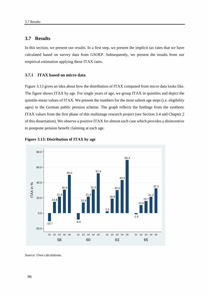
3.7 Results
96
3.7 Results
In this section, we present our results. In a first step, we present the implicit tax rates that we have
calculated based on survey data from GSOEP. Subsequently, we present the results from our
empirical estimation applying these ITAX rates.
3.7.1 ITAX based on micro data
Figure 3.13 gives an idea about how the distribution of ITAX computed from micro data looks like.
The figure shows ITAX by age. For single years of age, we group ITAX in quintiles and depict the
quintile-mean values of ITAX. We present the numbers for the most salient age steps (i.e. eligibility
ages) in the German public pension scheme. The graph reflects the findings from the synthetic
ITAX values from the first phase of this multistage research project (see Section 3.4 and Chapter 2
of this dissertation). We observe a positive ITAX for almost each case which provides a disincentive
to postpone pension benefit claiming at each age.
Figure 3.13: Distribution of ITAX by age
Source: Own calculations.
-10.7
14.8
21.6
30.6
50.0
-8.4
13.9
21.6
31.0
51.9
2.3
18.9
30.0
43.2
69.4
-1.6
10.515.7
21.2
32.3
-20.0
0.0
20.0
40.0
60.0
80.0
ITAX
in %
58 60 63 65Q1 Q2 Q3 Q4 Q5 Q1 Q2 Q3 Q4 Q5 Q1 Q2 Q3 Q4 Q5 Q1 Q2 Q3 Q4 Q5
3. Retirement Decisions in Germany: Micro-Modelling
97
3.7.2 Empirical estimation
3.7.2.1 The retirement model
Our outcome variable is labor force status in old age. It takes the value zero when the individual is
in the labor force, and value one when they are retired. As explained above, we will simply model
the transition from being in the labor force (full- or part-time) to being fully retired, as flexible
retirement is relatively rare in Germany. We assume that retirement is an absorbing state; therefore,
individuals are kept in the regression sample only until the first observation in retirement, and are
dropped from the sample afterwards. Thus, we can interpret our dependent variable as the
probability to retire in a given year, provided that the individual has been working in the previous
year.
Our main explanatory variable will be one of the two incentive variables described in Section 3.4:
accrual rate (the accrual divided by the level of social security wealth) and implicit tax rate. This
reduced form model of retirement has been extensively used in the literature along with different
incentive measures, for example the option value and the peak value (see, among others, Coile and
Gruber 2001 and Gruber and Wise 2004). The main difference with respect to measures like accrual
or ITAX is that the latter are one-year forward measures, whereas option value and peak value are
forward-looking measures, where the individual looks forward to the optimal retirement year, rather
than just to next year. However, as workers may be not completely forward-thinking or may be
unwilling to postpone retirement for too many years, the incentive measures we are using may be
considered appropriate.
A crucial issue in the analysis of retirement “is identification - that is, determination of the separate
effect of each variable on retirement, as distinct from each of the other variables” (Gruber and
Wise 2004). Indeed, in order to determine the effect of social security or pension incentives on
retirement, one needs to be able to separate the pure effect of economic incentives from the other
determinants of SSW, for example age and income. Controlling for these other determinants is
important if they are also independently correlated with retirement choices. However, there may be
a trade-off to take into account when introducing other control variables, as their estimated effect
may capture part of the effect pertaining to financial incentives, rather than individual heterogeneity,
thus leading to an underestimation of the incentives themselves. For this reason, exogenous
variation of financial incentives is important for identification. In this respect, Germany represents
a particularly well suited setting, given the various reforms and minor changes of the pension system
that were presented in Section 3.2. Furthermore, as first observed by Hurd (1990) and then reiterated

3.7 Results
98
by Coile and Gruber (2001) “if there are significant nonlinearities and interactions otherwise (likely)
uncorrelated with retirement that primarily identify the impact of these incentive measures, one
might feel more confident about retirement estimates”.
In the following regressions, households are divided into single households, meaning either non-
married individuals or single-earner households, and couple households, meaning households with
two earners or one earner and one retired spouse.32 Furthermore, we will show results separately
for men and women. Besides the main incentive variables, we will run regressions with and without
including a measure of individuals’ position in the lifetime earnings distribution (calculated as the
cumulative sum of earnings points, EP, divided by the length of the working life), as well as a
number of control variables: number of children, dummies for low and medium education, ISCO
code (one-digit classification of occupation), health satisfaction (from 0-low to 10-high), a dummy
for home ownership, and a dummy for working full-time. As displayed clearly in Figure 3.7, the
retirement probability by age is characterized by peaks in correspondence of the pension eligibility
ages. This may be due to liquidity constraints or social norms, the effects of which are not taken
into account by our constructed incentives measure. In order to address this concern, we will include
age dummies in all regressions.
Our main analysis is based on a random effects probit model. We will, however, also show the
robustness of our results by the use of alternative models, in particular: linear probability model
(LPM), random effects linear probability model (RE-LPM), fixed effects linear probability model
(FE-LPM), and probit model. In all models, standard errors are clustered at the individual level.
32 We include couples with one retired spouse in the group of couple households because the pension of the retired spouse enters the calculation of the working spouse’s ITAX through total household income.
3. Retirement Decisions in Germany: Micro-Modelling
99
3.7.2.2 Estimation results
Our main results are shown in Table 3.3 to Table 3.6, where we report marginal effects for the
explanatory variables of interest. As the accrual rate captures the substitution effect on retirement
decision from foregone future labor income, we expect the sign of this incentive to be negative: the
greater the foregone opportunities, the less likely workers are to retire. On the contrary, we expect
the sign of ITAX to be positive, as ITAX is defined as the negative accrual of social security wealth
divided by the after tax earnings during the additional year of work.
In almost all groups and specifications, we obtain the expected incentives signs. In all
specifications where the sign goes in the wrong direction, the corresponding coefficient is not
significant (accrual in the single-males specification (3), ITAX in the single males and females
specification (1) and (2)). In general, results for couples are more satisfactory than results for
singles, as coefficients are more often found to be statistically significant and are more robust to the
inclusion of average EP and other control variables. This might depend, among other things, on the
larger sample sizes.
Overall, our results point to a generally statistically insignificant effect of accrual rate for single
households, and a positive and statistically significant effect of ITAX for single females. If we
concentrate on the full specification, a ten percentage point increase in ITAX determines an increase
in the probability of retirement of 1.22 percentage points (pps) for females (see Table 3.5). In
regards to couples, a ten pps increase in the accrual rate determines a 3.9 pps increase in the
probability of retirement for males, while the effect of this incentive is not statistically significant
for females when control variables are included. A ten pps increase in ITAX is instead found to
increase males’ probability of retirement by 1.1 pps, and females’ probability by 0.6 pps.
In Table 3.7 to Table 3.10, we check the robustness of these results using different models. For
the sake of space, in these tables we concentrate on the full specification that includes all control
variables. In general, results are rather robust. LPM and RE-LPM deliver almost exactly the same
results, and both seem to underestimate the effect of the incentives that we find using the RE probit
model. Similarly, probit and RE probit also deliver almost exactly the same results.
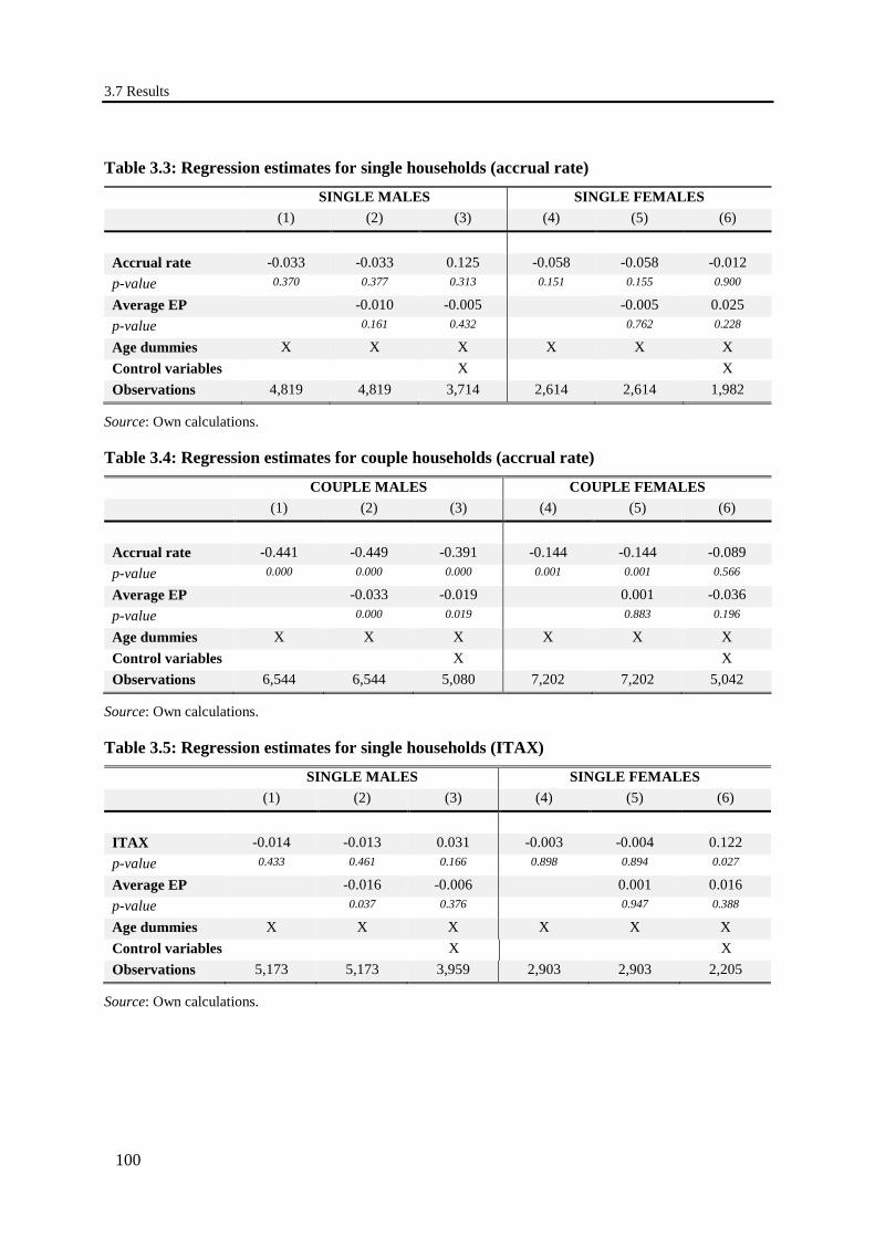
3.7 Results
100
Table 3.3: Regression estimates for single households (accrual rate)
SINGLE MALES SINGLE FEMALES (1) (2) (3) (4) (5) (6)
Accrual rate -0.033 -0.033 0.125 -0.058 -0.058 -0.012 p-value 0.370 0.377 0.313 0.151 0.155 0.900
Average EP
-0.010 -0.005
-0.005 0.025 p-value
0.161 0.432
0.762 0.228
Age dummies X X X X X X Control variables
X
X
Observations 4,819 4,819 3,714 2,614 2,614 1,982
Source: Own calculations.
Table 3.4: Regression estimates for couple households (accrual rate)
COUPLE MALES COUPLE FEMALES (1) (2) (3) (4) (5) (6)
Accrual rate -0.441 -0.449 -0.391 -0.144 -0.144 -0.089 p-value 0.000 0.000 0.000 0.001 0.001 0.566
Average EP
-0.033 -0.019
0.001 -0.036 p-value
0.000 0.019
0.883 0.196
Age dummies X X X X X X Control variables
X
X
Observations 6,544 6,544 5,080 7,202 7,202 5,042
Source: Own calculations.
Table 3.5: Regression estimates for single households (ITAX)
SINGLE MALES SINGLE FEMALES (1) (2) (3) (4) (5) (6)
ITAX -0.014 -0.013 0.031 -0.003 -0.004 0.122 p-value 0.433 0.461 0.166 0.898 0.894 0.027
Average EP
-0.016 -0.006
0.001 0.016 p-value
0.037 0.376
0.947 0.388
Age dummies X X X X X X Control variables
X
X
Observations 5,173 5,173 3,959 2,903 2,903 2,205
Source: Own calculations.
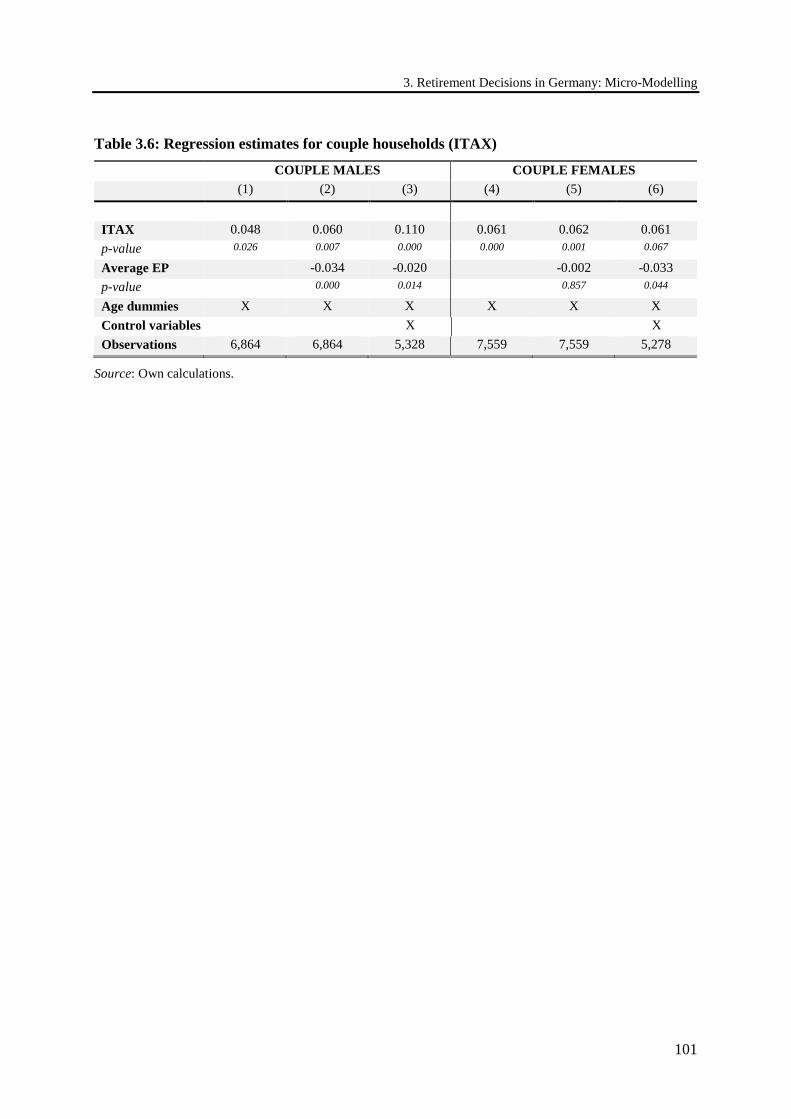
3. Retirement Decisions in Germany: Micro-Modelling
101
Table 3.6: Regression estimates for couple households (ITAX)
COUPLE MALES COUPLE FEMALES (1) (2) (3) (4) (5) (6)
ITAX 0.048 0.060 0.110 0.061 0.062 0.061 p-value 0.026 0.007 0.000 0.000 0.001 0.067
Average EP
-0.034 -0.020
-0.002 -0.033 p-value
0.000 0.014
0.857 0.044
Age dummies X X X X X X Control variables
X
X
Observations 6,864 6,864 5,328 7,559 7,559 5,278
Source: Own calculations.
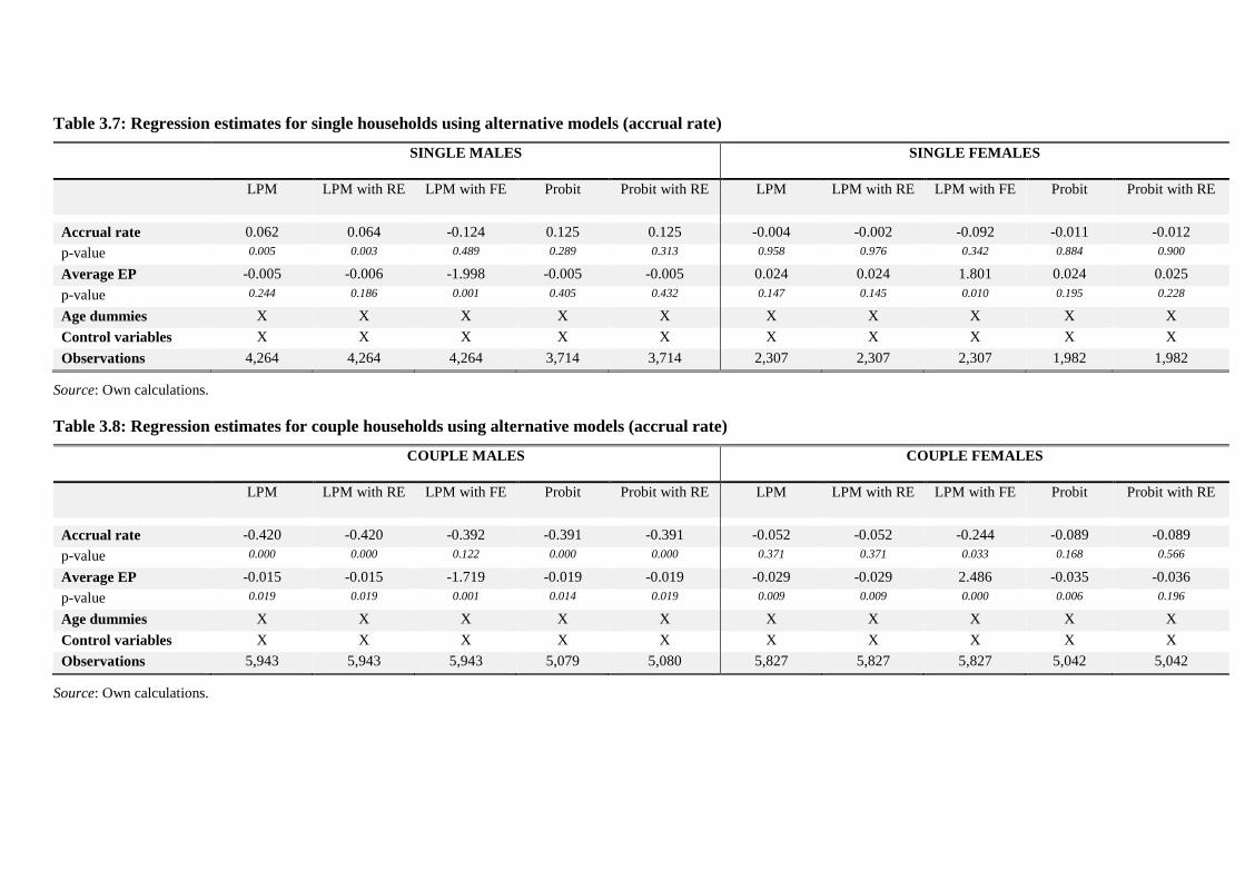
Table 3.7: Regression estimates for single households using alternative models (accrual rate)
SINGLE MALES SINGLE FEMALES
LPM LPM with RE LPM with FE Probit Probit with RE LPM LPM with RE LPM with FE Probit Probit with RE
Accrual rate 0.062 0.064 -0.124 0.125 0.125 -0.004 -0.002 -0.092 -0.011 -0.012 p-value 0.005 0.003 0.489 0.289 0.313 0.958 0.976 0.342 0.884 0.900
Average EP -0.005 -0.006 -1.998 -0.005 -0.005 0.024 0.024 1.801 0.024 0.025 p-value 0.244 0.186 0.001 0.405 0.432 0.147 0.145 0.010 0.195 0.228
Age dummies X X X X X X X X X X Control variables X X X X X X X X X X Observations 4,264 4,264 4,264 3,714 3,714 2,307 2,307 2,307 1,982 1,982
Source: Own calculations.
Table 3.8: Regression estimates for couple households using alternative models (accrual rate)
COUPLE MALES COUPLE FEMALES
LPM LPM with RE LPM with FE Probit Probit with RE LPM LPM with RE LPM with FE Probit Probit with RE
Accrual rate -0.420 -0.420 -0.392 -0.391 -0.391 -0.052 -0.052 -0.244 -0.089 -0.089 p-value 0.000 0.000 0.122 0.000 0.000 0.371 0.371 0.033 0.168 0.566
Average EP -0.015 -0.015 -1.719 -0.019 -0.019 -0.029 -0.029 2.486 -0.035 -0.036 p-value 0.019 0.019 0.001 0.014 0.019 0.009 0.009 0.000 0.006 0.196
Age dummies X X X X X X X X X X Control variables X X X X X X X X X X Observations 5,943 5,943 5,943 5,079 5,080 5,827 5,827 5,827 5,042 5,042
Source: Own calculations.
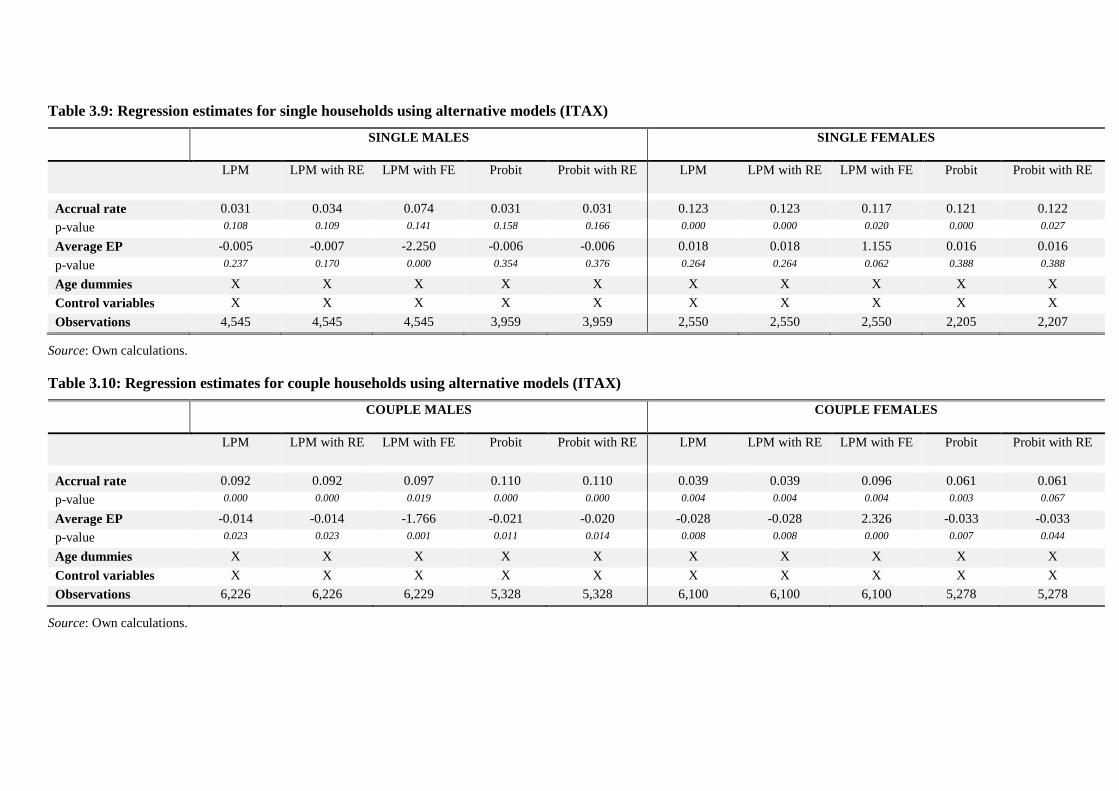
103
Table 3.9: Regression estimates for single households using alternative models (ITAX)
SINGLE MALES SINGLE FEMALES
LPM LPM with RE LPM with FE Probit Probit with RE LPM LPM with RE LPM with FE Probit Probit with RE
Accrual rate 0.031 0.034 0.074 0.031 0.031 0.123 0.123 0.117 0.121 0.122 p-value 0.108 0.109 0.141 0.158 0.166 0.000 0.000 0.020 0.000 0.027
Average EP -0.005 -0.007 -2.250 -0.006 -0.006 0.018 0.018 1.155 0.016 0.016 p-value 0.237 0.170 0.000 0.354 0.376 0.264 0.264 0.062 0.388 0.388
Age dummies X X X X X X X X X X Control variables X X X X X X X X X X Observations 4,545 4,545 4,545 3,959 3,959 2,550 2,550 2,550 2,205 2,207
Source: Own calculations.
Table 3.10: Regression estimates for couple households using alternative models (ITAX)
COUPLE MALES COUPLE FEMALES
LPM LPM with RE LPM with FE Probit Probit with RE LPM LPM with RE LPM with FE Probit Probit with RE
Accrual rate 0.092 0.092 0.097 0.110 0.110 0.039 0.039 0.096 0.061 0.061 p-value 0.000 0.000 0.019 0.000 0.000 0.004 0.004 0.004 0.003 0.067
Average EP -0.014 -0.014 -1.766 -0.021 -0.020 -0.028 -0.028 2.326 -0.033 -0.033 p-value 0.023 0.023 0.001 0.011 0.014 0.008 0.008 0.000 0.007 0.044
Age dummies X X X X X X X X X X Control variables X X X X X X X X X X Observations 6,226 6,226 6,229 5,328 5,328 6,100 6,100 6,100 5,278 5,278
Source: Own calculations.
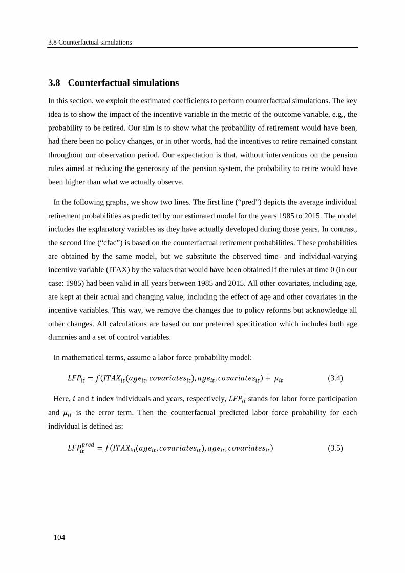
3.8 Counterfactual simulations
104
3.8 Counterfactual simulations
In this section, we exploit the estimated coefficients to perform counterfactual simulations. The key
idea is to show the impact of the incentive variable in the metric of the outcome variable, e.g., the
probability to be retired. Our aim is to show what the probability of retirement would have been,
had there been no policy changes, or in other words, had the incentives to retire remained constant
throughout our observation period. Our expectation is that, without interventions on the pension
rules aimed at reducing the generosity of the pension system, the probability to retire would have
been higher than what we actually observe.
In the following graphs, we show two lines. The first line (“pred”) depicts the average individual
retirement probabilities as predicted by our estimated model for the years 1985 to 2015. The model
includes the explanatory variables as they have actually developed during those years. In contrast,
the second line (“cfac”) is based on the counterfactual retirement probabilities. These probabilities
are obtained by the same model, but we substitute the observed time- and individual-varying
incentive variable (ITAX) by the values that would have been obtained if the rules at time 0 (in our
case: 1985) had been valid in all years between 1985 and 2015. All other covariates, including age,
are kept at their actual and changing value, including the effect of age and other covariates in the
incentive variables. This way, we remove the changes due to policy reforms but acknowledge all
other changes. All calculations are based on our preferred specification which includes both age
dummies and a set of control variables.
In mathematical terms, assume a labor force probability model:
𝐿𝐿𝐿𝐿𝐸𝐸𝑖𝑖𝑡𝑡 = 𝑓𝑓(𝐼𝐼𝐼𝐼𝐼𝐼𝐼𝐼𝑖𝑖𝑡𝑡(𝑎𝑎𝑎𝑎𝑎𝑎𝑖𝑖𝑡𝑡 , 𝑐𝑐𝑐𝑐𝑐𝑐𝑎𝑎𝑟𝑟𝑖𝑖𝑎𝑎𝑝𝑝𝑎𝑎𝑐𝑐𝑖𝑖𝑡𝑡),𝑎𝑎𝑎𝑎𝑎𝑎𝑖𝑖𝑡𝑡 , 𝑐𝑐𝑐𝑐𝑐𝑐𝑎𝑎𝑟𝑟𝑖𝑖𝑎𝑎𝑝𝑝𝑎𝑎𝑐𝑐𝑖𝑖𝑡𝑡) + 𝜇𝜇𝑖𝑖𝑡𝑡 (3.4)
Here, 𝑖𝑖 and 𝑝𝑝 index individuals and years, respectively, 𝐿𝐿𝐿𝐿𝐸𝐸𝑖𝑖𝑡𝑡 stands for labor force participation
and 𝜇𝜇𝑖𝑖𝑡𝑡 is the error term. Then the counterfactual predicted labor force probability for each
individual is defined as:
𝐿𝐿𝐿𝐿𝐸𝐸𝑖𝑖𝑡𝑡𝑝𝑝𝑝𝑝𝑁𝑁𝑝𝑝 = 𝑓𝑓(𝐼𝐼𝐼𝐼𝐼𝐼𝐼𝐼𝑖𝑖0(𝑎𝑎𝑎𝑎𝑎𝑎𝑖𝑖𝑡𝑡 , 𝑐𝑐𝑐𝑐𝑐𝑐𝑎𝑎𝑟𝑟𝑖𝑖𝑎𝑎𝑝𝑝𝑎𝑎𝑐𝑐𝑖𝑖𝑡𝑡), 𝑎𝑎𝑎𝑎𝑎𝑎𝑖𝑖𝑡𝑡 , 𝑐𝑐𝑐𝑐𝑐𝑐𝑎𝑎𝑟𝑟𝑖𝑖𝑎𝑎𝑝𝑝𝑎𝑎𝑐𝑐𝑖𝑖𝑡𝑡) (3.5)
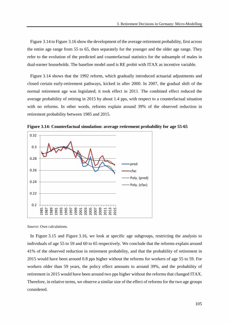
3. Retirement Decisions in Germany: Micro-Modelling
105
Figure 3.14 to Figure 3.16 show the development of the average retirement probability, first across
the entire age range from 55 to 65, then separately for the younger and the older age range. They
refer to the evolution of the predicted and counterfactual statistics for the subsample of males in
dual-earner households. The baseline model used is RE probit with ITAX as incentive variable.
Figure 3.14 shows that the 1992 reform, which gradually introduced actuarial adjustments and
closed certain early-retirement pathways, kicked in after 2000. In 2007, the gradual shift of the
normal retirement age was legislated; it took effect in 2011. The combined effect reduced the
average probability of retiring in 2015 by about 1.4 pps, with respect to a counterfactual situation
with no reforms. In other words, reforms explain around 39% of the observed reduction in
retirement probability between 1985 and 2015.
Figure 3.14: Counterfactual simulation: average retirement probability for age 55-65
Source: Own calculations.
In Figure 3.15 and Figure 3.16, we look at specific age subgroups, restricting the analysis to
individuals of age 55 to 59 and 60 to 65 respectively. We conclude that the reforms explain around
41% of the observed reduction in retirement probability, and that the probability of retirement in
2015 would have been around 0.8 pps higher without the reforms for workers of age 55 to 59. For
workers older than 59 years, the policy effect amounts to around 39%, and the probability of
retirement in 2015 would have been around two pps higher without the reforms that changed ITAX.
Therefore, in relative terms, we observe a similar size of the effect of reforms for the two age groups
considered.
0.2
0.22
0.24
0.26
0.28
0.3
0.32
1985
1987
1989
1991
1993
1995
1997
1999
2001
2003
2005
2007
2009
2011
2013
2015
pred
cfac
Poly. (pred)
Poly. (cfac)
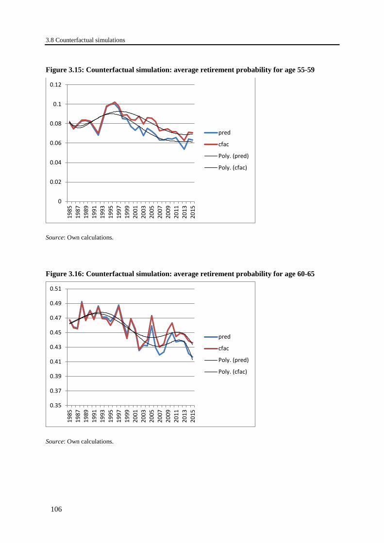
3.8 Counterfactual simulations
106
Figure 3.15: Counterfactual simulation: average retirement probability for age 55-59
Source: Own calculations.
Figure 3.16: Counterfactual simulation: average retirement probability for age 60-65
Source: Own calculations.
0
0.02
0.04
0.06
0.08
0.1
0.12
1985
1987
1989
1991
1993
1995
1997
1999
2001
2003
2005
2007
2009
2011
2013
2015
pred
cfac
Poly. (pred)
Poly. (cfac)
0.35
0.37
0.39
0.41
0.43
0.45
0.47
0.49
0.51
1985
1987
1989
1991
1993
1995
1997
1999
2001
2003
2005
2007
2009
2011
2013
2015
pred
cfac
Poly. (pred)
Poly. (cfac)
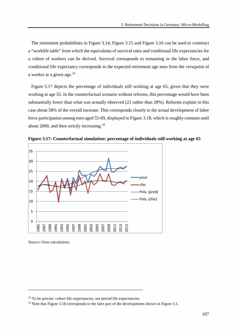
3. Retirement Decisions in Germany: Micro-Modelling
107
The retirement probabilities in Figure 3.14, Figure 3.15 and Figure 3.16 can be used to construct
a “worklife table” from which the equivalents of survival rates and conditional life expectancies for
a cohort of workers can be derived. Survival corresponds to remaining in the labor force, and
conditional life expectancy corresponds to the expected retirement age seen from the viewpoint of
a worker at a given age.33
Figure 3.17 depicts the percentage of individuals still working at age 65, given that they were
working at age 55. In the counterfactual scenario without reforms, this percentage would have been
substantially lower than what was actually observed (21 rather than 28%). Reforms explain in this
case about 58% of the overall increase. This corresponds closely to the actual development of labor
force participation among men aged 55-69, displayed in Figure 3.18, which is roughly constant until
about 2000, and then strictly increasing.34
Figure 3.17: Counterfactual simulation: percentage of individuals still working at age 65
Source: Own calculations.
33 To be precise: cohort life expectancies, not period life expectancies. 34 Note that Figure 3.18 corresponds to the later part of the developments shown in Figure 3.1.
0
5
10
15
20
25
30
35
1985
1987
1989
1991
1993
1995
1997
1999
2001
2003
2005
2007
2009
2011
2013
2015
pred
cfac
Poly. (pred)
Poly. (cfac)
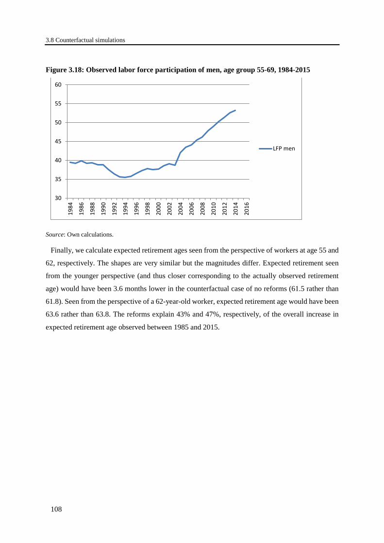
3.8 Counterfactual simulations
108
Figure 3.18: Observed labor force participation of men, age group 55-69, 1984-2015
Source: Own calculations.
Finally, we calculate expected retirement ages seen from the perspective of workers at age 55 and
62, respectively. The shapes are very similar but the magnitudes differ. Expected retirement seen
from the younger perspective (and thus closer corresponding to the actually observed retirement
age) would have been 3.6 months lower in the counterfactual case of no reforms (61.5 rather than
61.8). Seen from the perspective of a 62-year-old worker, expected retirement age would have been
63.6 rather than 63.8. The reforms explain 43% and 47%, respectively, of the overall increase in
expected retirement age observed between 1985 and 2015.
30
35
40
45
50
55
60
1984
1986
1988
1990
1992
1994
1996
1998
2000
2002
2004
2006
2008
2010
2012
2014
2016
LFP men
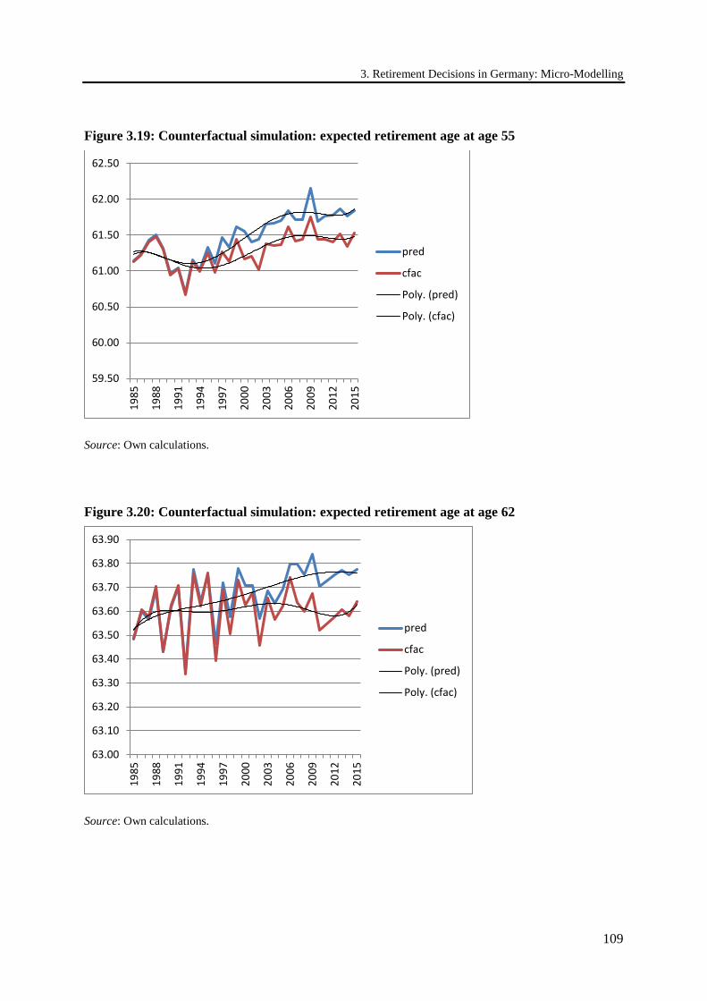
3. Retirement Decisions in Germany: Micro-Modelling
109
Figure 3.19: Counterfactual simulation: expected retirement age at age 55
Source: Own calculations.
Figure 3.20: Counterfactual simulation: expected retirement age at age 62
Source: Own calculations.
59.50
60.00
60.50
61.00
61.50
62.00
62.50
1985
1988
1991
1994
1997
2000
2003
2006
2009
2012
2015
pred
cfac
Poly. (pred)
Poly. (cfac)
63.00
63.10
63.20
63.30
63.40
63.50
63.60
63.70
63.80
63.90
1985
1988
1991
1994
1997
2000
2003
2006
2009
2012
2015
pred
cfac
Poly. (pred)
Poly. (cfac)
3.9 Conclusions
110
3.9 Conclusions
Employment of older individuals in Germany has experienced a remarkable reversal around the late
1990s. After a long declining trend that began in the early 1970s, the employment rate for older
men has strongly increased again. This increase has lasted until today. This chapter uses micro data
from the German Socio-Economic Panel in order to link these labor market trends to changes in
public pension policies, especially the change in the incentive variables ITAX, the implicit tax on
working longer, using various regression models.
Our model produced predicted retirement probabilities for each sample person and how this has
changed from 1985 to 2015. We also used this model to compute counterfactual retirement
probabilities, i.e., estimates of how retirement probabilities would have changed if public pension
policies in Germany had remained unchanged after 1985. The difference between the counterfactual
retirement probabilities and the predicted baseline probabilities can be interpreted as the causal
effect of the sequence of pension reforms that took place between 1985 and 2015 in Germany.
We find that for men in couple households the predicted and counterfactual retirement
probabilities start to deviate from each other after about the year 2000. This coincides with the
introduction of the actuarial deductions as legislated in the 1992 reform. We also find that our model
relates an increase of about 0.3 years in the average retirement age to the reform-driven change of
the implicit tax on working longer. This is substantially less than the actual increase which was
around 1.5 years.35 One reason may be that ITAX only captures part of the changed policy
environment. Other parts of this environment include the general awareness of population aging
and related or unrelated changes in the preference for work vs. leisure in the age range under
consideration. Moreover, the closure of entire pathways such as the pathway for women and the
pathway for unemployment may only partially be reflected in the construction of our main incentive
variable ITAX.
This paper only observes labor supply reactions until 2015, the last year of our data. We therefore
do not observe reactions to further changes that have already been legislated, especially the gradual
increase of the retirement age which will last until 2030. Future research has to show whether this
gradual change will increase the actual retirement age in Germany even further.
35 Actual retirement age for men was 62.5 in 1980 and 64 in 2015.
111
4. Dangerous Flexibility – Retirement Reforms Reconsidered
This chapter was written in co-authorship with Axel Börsch-Supan, Tabea Bucher-Koenen and
Vesile Kutlu Koc.
4.1 Introduction
In the face of aging societies, there is an on-going debate in many countries around the world on
how to make pension systems more sustainable. The combination of rising life expectancy and low
fertility rates, as well as the retirement of the baby boomers, are putting pressure on pension
systems. In order to ease the burden of demographic change, a common objective in many
developed economies is to better tap into the pool of older workers.
Increasing the statutory retirement age is an obvious and effective policy to achieve this objective.
Later retirement has two effects which help to stabilize the financial situation of pension systems:
it reduces the volume of pension benefits to be paid and it increases the total labor volume that
constitutes the tax and contribution base to finance the pension system.
Increasing the retirement age, however, is not a very popular policy. Politicians often consider
reforms which are designed to make pension systems more sustainable and resilient against
population aging as the “third rail in politics”, referring to the high-voltage rail in the subway which
gives a fatal jolt to those who touch it (Safire 2007, Lynch and Myrskyl 2009). Increasing the
retirement age appears to carry a particularly high voltage.
Politicians therefore have invented a new kid in the town of retirement policies called “flexibility
reforms”. They are designed to allow workers to retire more “flexibly”, “gradually” or “partially”
as a seemingly elegant way to increase older workers’ labor supply by relaxing constraints such as
4.1 Introduction
112
mandatory retirement, earnings tests which effectively impose maximum hours constraints and
minimum hours constraints, and by introducing partial retirement, a combination of part-time work
and pension benefit receipt.
While flexible retirement policies may have intuitive appeal to policy makers and the populace in
general, this study argues that they are dangerous instruments because they are likely to exert
counteracting incentives when they are applied to the currently existing public pension systems.
Economic theory shows that – while some workers who retire early without the availability of the
part-time option might extend their working lives on a part-time schedule – others might opt for
part-time work instead of full-time work and thus reduce their total hours worked. It is therefore an
empirical question whether flexible retirement can be a successful policy alternative to a later
statutory retirement age. Our empirical results shed serious doubts on this. At best, recent flexibility
reforms show no significant effects on total labor volume; in many cases, however, they decreased
it. If neutral, flexibility reforms are dangerous because they postpone or replace more effective
policies such as increasing the statutory retirement age. Even larger are the dangers if they actually
reduce total labor volume supplied by older workers – as they have in many countries – and thereby
weaken the financial base of pension systems rather than strengthening it.
There is not much research on this issue. Previous work focuses on the effect of a particular reform
in a specific country (see, e.g., Graf et al. 2011 for evidence on Austria, Huber et al. 2013 for
evidence on Germany, Ilmakunnas and Ilmakunnas 2006 for evidence on Finland, and Brinch et al.
2015 for evidence on Norway). Gustman and Steinmeier (1983) study the presence and rationale
for minimum hours constraints and cite empirical evidence that this is particularly salient for the
US. They show that a minimum hours constraint changes retirement behavior since older workers
may prefer part-time but are forced to decide between full-time work and full-time retirement. The
dynamic programming model by Gustman and Steinmeier (1984, 1986, 2004) predicts that the
typical minimum hours constraint in the US generates earlier retirement than in the case of
unrestricted hours. There are also restrictions on the maximum amount of labor that households
may supply. The most prominent examples are earnings tests which distort labor supply at older
ages in many countries (Börsch-Supan et al. 2017). Further studies show that older workers would
prefer to reduce their working hours towards their retirement as an alternative to fully retiring
(Gielen 2009, Büsch et al. 2010, Cihlar et al. 2014 for evidence on Germany).
We employ an internationally comparative view to study the effect of flexibility reforms. We
collect evidence of different reform measures taken in various countries at different times. We use
4. Dangerous Flexibility – Retirement Reforms Reconsidered
113
the pooled cross-national and intertemporal variance in pension rules to identify the effects of the
flexibility reforms on the total labor supply of older workers. We use aggregate time series data
from the OECD’s employment database for a subsample of nine OECD countries which introduced
flexible retirement reforms in the past, namely Australia, Austria, Belgium, Denmark, Finland,
France, Germany, The Netherlands, and Sweden. Using this sample, we first estimate the effect of
flexible retirement on labor force participation (extensive margin) and then on working hours of
older workers (intensive margin). Our distinction between the intensive and the extensive margin is
an important feature of this study. So far most of the studies evaluating the effects of flexibility
reforms on labor supply have focused on the extensive margin. We will show that more flexibility
can increase the overall labor force participation (extensive margin). At the same time, however,
more flexibility can decrease the average hours worked (intensive margin), potentially decreasing
total labor volume.
The chapter proceeds as follows: Section 4.2 presents stylized facts about labor force participation
of older workers in the countries under investigation. Section 4.3 summarizes the flexible retirement
schemes that have been introduced in the countries which we study. Section 4.4 provides the
theoretical reasoning and shows that the overall effect of a reform allowing for more flexible
transitions to retirement on total labor supply is ex ante unclear. The empirical analysis in
Section 4.5 documents that the potentially unpleasant effects predicted by the theoretical analysis
have indeed happened in many countries. We therefore conclude in Section 4.6 that the flexibility
reforms enacted so far have failed to be an effective policy to increase the labor supply of older
workers. While they might increase utility for current retirees, they are dangerous if they replace
more effective policies or decrease total labor volume and thus increase the financial burden for the
younger generation.
4.2 Labor supply and retirement patterns
The statutory retirement age – more precisely named the statutory eligibility age (SEA) as it defines
the age at which workers are eligible for full pension benefits independent of any other
qualification – sends a strong signal to older workers to leave the labor force. This is shown in
Figure 4.1.36 Most workers have left the labor force when they have reached the statutory eligibility
36 The study concentrates on the labor supply of men age 55 and over. In most countries considered, female labor force participation of the equivalent cohorts has been low with a large share of part-time work at younger ages, making these women ineligible for most of the reforms considered later in this analysis.
4.2 Labor supply and retirement patterns
114
age, and the average exit age (AEA) from the labor force is considerably lower than the statutory
eligibility age. This pattern is similar among the European countries. Only for males in Sweden, the
average exit age is later than the statutory eligibility age. In all countries, the labor force profiles
exhibit a rather steep slope during the period shortly before the statutory retirement age.
From an economist’s perspective, the existence of a fixed and universal retirement age needs
explanation since preferences for leisure differ between individuals and over age, health at older
ages varies widely and family circumstances such as the need to take care of parents or a partner
differ across households especially at older ages. Moreover, there is no economic reason why
claiming a pension must imply leaving the labor force. When to claim a contributory pension should
depend on actuarial rules while when to exit the labor force should depend on the preference for
leisure. Hence, the exit from the labor force could occur earlier, at the same time or later than
claiming a pension. However, in many cases, this flexibility is restricted by a combination of
constraints and incentives imposed by employers, unions and governments. Flexibility reforms try
to reduce these constraints.
First, in many sectors of European countries the statutory eligibility age is effectively a mandatory
retirement age. This is usually not a legal constraint but determined in labor agreements between
the social parties. Unions have traditionally pursued a policy of pushing for an early retirement age
and justified this by protecting workers with declining health and (misleadingly so) by freeing up
jobs for younger workers. Employers, as pointed out already very early by Gustman and Steinmeier
(1983), like to impose a lower limit on the hours worked since part-time jobs and flexible hours
incur additional fixed costs of work.37 As a consequence, and in contrast to standard labor market
theory, many workers are not free to choose their working hours, in this case to reduce their working
hours when they become older but must choose between working full-time or retiring fully.
Second, many pension systems impose earnings tests which limit the amount of earnings that can
be received by an individual who receives pension benefits. They usually concern the time period
before reaching the statutory eligibility age. Again, this is an impediment for flexible retirement
since earnings tests impose a maximum hours constraint for a given wage. As Table A.1.1
(Appendix to Chapter 4) shows, the maximum permissible earnings are relatively low and in many
cases (e.g. in Austria, Belgium and Germany) are substantially below a half-time job. In
37 Fixed costs of employment and team production are some of the reasons why minimum hours constraints exist. See Gustman and Steinmeier (1983) and Hurd (1996) for other possible reasons.
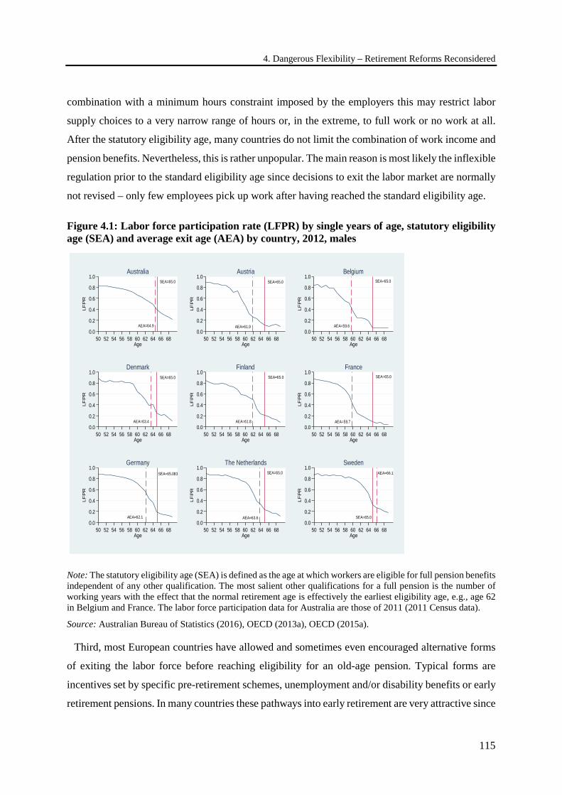
4. Dangerous Flexibility – Retirement Reforms Reconsidered
115
combination with a minimum hours constraint imposed by the employers this may restrict labor
supply choices to a very narrow range of hours or, in the extreme, to full work or no work at all.
After the statutory eligibility age, many countries do not limit the combination of work income and
pension benefits. Nevertheless, this is rather unpopular. The main reason is most likely the inflexible
regulation prior to the standard eligibility age since decisions to exit the labor market are normally
not revised – only few employees pick up work after having reached the standard eligibility age.
Figure 4.1: Labor force participation rate (LFPR) by single years of age, statutory eligibility age (SEA) and average exit age (AEA) by country, 2012, males
Note: The statutory eligibility age (SEA) is defined as the age at which workers are eligible for full pension benefits independent of any other qualification. The most salient other qualifications for a full pension is the number of working years with the effect that the normal retirement age is effectively the earliest eligibility age, e.g., age 62 in Belgium and France. The labor force participation data for Australia are those of 2011 (2011 Census data).
Source: Australian Bureau of Statistics (2016), OECD (2013a), OECD (2015a).
Third, most European countries have allowed and sometimes even encouraged alternative forms
of exiting the labor force before reaching eligibility for an old-age pension. Typical forms are
incentives set by specific pre-retirement schemes, unemployment and/or disability benefits or early
retirement pensions. In many countries these pathways into early retirement are very attractive since
SEA=65.0
AEA=64.90.0
0.2
0.4
0.6
0.8
1.0
LFP
R
50 52 54 56 58 60 62 64 66 68Age
AustraliaSEA=65.0
AEA=61.90.0
0.2
0.4
0.6
0.8
1.0
LFP
R
50 52 54 56 58 60 62 64 66 68Age
AustriaSEA=65.0
AEA=59.60.0
0.2
0.4
0.6
0.8
1.0
LFP
R
50 52 54 56 58 60 62 64 66 68Age
Belgium
SEA=65.0
AEA=63.40.0
0.2
0.4
0.6
0.8
1.0
LFP
R
50 52 54 56 58 60 62 64 66 68Age
DenmarkSEA=65.0
AEA=61.80.0
0.2
0.4
0.6
0.8
1.0
LFP
R
50 52 54 56 58 60 62 64 66 68Age
FinlandSEA=65.0
AEA=59.70.0
0.2
0.4
0.6
0.8
1.0
LFP
R
50 52 54 56 58 60 62 64 66 68Age
France
SEA=65.083
AEA=62.10.0
0.2
0.4
0.6
0.8
1.0
LFP
R
50 52 54 56 58 60 62 64 66 68Age
GermanySEA=65.0
AEA=63.60.0
0.2
0.4
0.6
0.8
1.0
LFP
R
50 52 54 56 58 60 62 64 66 68Age
The NetherlandsAEA=66.1
SEA=65.00.0
0.2
0.4
0.6
0.8
1.0
LFP
R
50 52 54 56 58 60 62 64 66 68Age
Sweden
4.3 Flexibility reforms
116
pension benefits are not calculated in an actuarially neutral way. This means that there exists an
implicit tax on working longer once individuals have reached the earliest eligibility age, thus
encouraging them to claim their pensions as early as possible (Gruber and Wise 1999, 2002).
The combination of these constraints and incentives tends to induce workers to both claim the
pension and exit the labor force at the earliest possible time. The two events then occur
simultaneously. This is reflected in the rapid and early decline in labor force participation in
Figure 4.1. The differences in the slopes reflect different preferences for leisure as well as
differences in early retirement incentives provided by the pension systems in each country and the
other impediments to flexibility that disrupt the bridge between exiting the labor force and eligibility
for a pension.
Institutional arrangements also influence the demand for labor at older ages: it might be optimal
for employers to discharge older workers when their productivity does not increase anymore but
labor contracts still impose rising wages. Moreover, in many countries it is much cheaper to dismiss
older rather than younger workers when a company is forced to restructure because severance
payments to older workers are effectively subsidized by early retirement and disability benefits
(Börsch-Supan et al. 2009). These mechanisms have also shaped the slopes visible in Figure 4.1.
We will, however, focus on the supply side in the sequel of the study.
4.3 Flexibility reforms
In the last two decades, most OECD countries have attempted a shift away from the different early
retirement policies mentioned in the previous section and moved towards a strategy of more active
aging and longer working lives. Many countries have undertaken substantial pension reforms which
have included flexible retirement schemes. The primary goals of these flexible retirement schemes
are, on the one hand, to enable employees to gradually reduce their working hours with increasing
age in order to facilitate the transition from full-time employment to full retirement. On the other
hand, older workers are encouraged to remain in the labor market as long as possible, preferably
beyond the statutory eligibility age. Since very often the minimum hours constraints by the
employers restrict the labor supply of older workers, in some countries the flexibility reforms
targeted firms and set incentives for them to offer part-time schemes to older workers by subsidizing
4. Dangerous Flexibility – Retirement Reforms Reconsidered
117
the wages of those workers under certain conditions. Table A.1.1 gives an overview of the flexibility
reforms that will be analyzed in Section 4.5 and summarizes their key parameters.38
A particularly interesting case is Sweden. With the 2000 pension reform that introduced the now
famous notional defined contribution system (Palmer 2000), Sweden also introduced a much more
flexible scheme regarding retirement entry. Since then, there is no formal retirement age any more.
In the new system, pensions can be drawn from age 61 onwards, without an upper age limit. Pension
entitlements accrue on individual notional accounts if the person earns pensionable income,
regardless of his or her age and irrespective whether the individual already gets a pension. Pension
payments are calculated by dividing the notional account balance by a cohort-specific annuity
divisor which is linked to the retirement age and the life expectancy of each cohort. The pension
payment increases with the age of retirement due to the resulting shorter period over which a
pension is paid. It is possible to combine an old-age pension with work income without any financial
restrictions or earnings test (Lindecke et al. 2007). Over time, an increasing number of Swedes has
begun to claim a pension at the age 61. While 3.9% of the 1939 cohort received a pension with 61,
the proportion increased to 5.9% in the 1949 cohort and 7.8% in the 1953 cohort. The persistent
trend to claim pension benefits as early as possible led to a debate in Sweden with the plan to raise
the minimum eligibility age from 61 to 63 (Statens Offentliga Utredningar 2013).
Already in 1992, Germany introduced a partial pension system. In compliance with certain
supplementary income limits, individuals could reduce their working hours by working part-time
and compensate the resulting income loss by drawing a partial pension. The pension contributions
payed on the reduced labor income led to higher pension entitlements later on. Eligibility for the
partial pension depended on being entitled to an old-age pension. The partial pension could only be
drawn for certain proportions of the split between work and retirement: either one third, one half,
or two thirds. In between, no further gradations were possible. The earning limits were calculated
individually based on the labor income of the last three years before drawing the partial pension.
This system of partial pensions, was not successful and only taken up by few individuals. In 1993,
the number of new partial pensioners was around 1,100; approaching 3,000 at the end of the 1990s
and declining thereafter. Since the introduction in 1992, the proportion of new pensioners claiming
a partial pension was below 0.5% in each year (Börsch-Supan et al. 2015). The rigid earnings limits
38 Norway, the UK and the US have also recently introduced flexibility reforms. Since those reforms were very recent, we do not have a sufficient number of post-reform observations for the empirical analysis and therefore do not describe those reforms here.
4.3 Flexibility reforms
118
were slightly increased in 2008 and finally substituted by a more flexible limit in 2016 which came
into force in July 2017.
In the early 1990s, but especially with the 1993 reform, the French government attempted to
reverse the previously widespread early retirement trend by promoting gradual retirement through
governmental subsidies. The partial retirement scheme was designed for employees from age 55 to
65. Employees could earn income based on their part-time work and in the time before full
retirement, receive a governmental income supplement equal to about 30% of the daily reference
wage (up to a ceiling). The firm had to hire a new employee for the vacant part-time position. At
the end of the 1990s, about 45,000 private-sector workers were benefitting from the governmental
subsidies within this partial retirement scheme. The scheme was abolished in 2004 (Reday-Mulvey
2000, OECD 2005a).
With the 1995 reform in Denmark, the government tried to encourage gradual retirement by
replacing the full early retirement system with a part-time work scheme. The system required that
the employee was aged between 60 and 66 years, was entitled to unemployment benefits and was a
member of an unemployment insurance fund for at least 20 out of the last 25 years. Within the
scheme, working time had to be reduced by at least 25% (or by 18.5 hours per week for self-
employed), but the remaining working time should be at least twelve hours a week. The income
loss was compensated by a fixed payment of the unemployment insurance fund which was in 1995
7.67€ per hour of working time reduction (2016: 12.32€). The unemployment insurance fund
administered the scheme (European Commission 1995, Delsen 1996, Eurofound 2016). Hansen
(2001) states that the scheme never attracted many participants; in the late 1990s there were around
1,000 partial pensioners per year. The scheme is being phased out (OECD 2011a).
In Austria, a subsidized old-age part-time scheme was introduced in 2000. The scheme is based
on a bilateral agreement between the employer and the employee and requires a reduction of
working hours between 40% and 60%. Working time can be distributed in two distinctly different
ways: Either the employee reduces his working hours for the whole period of 6.5 years by half or
the “block model” option can be chosen. In this option the employee continues working without
any reduction in working hours for the first part of the period (first block), while for the second
period (second block), the employee stops working completely. Employees must have worked at
least 80% of a regular full-time employment, before they are entitled to the subsidized scheme. 50%
of the income loss is compensated by governmental subsidies, up to 75% of the former gross wage.
Pension contributions have to be paid at the same amount as before the working time reduction. In
4. Dangerous Flexibility – Retirement Reforms Reconsidered
119
2000, the lower age limit of the flexible retirement window was 50 for women and 55 for men. In
2005, this was increased to 52 for women and 57 for men, and further to 55 and 60 in 2013. In 2001,
5,274 individuals were part of the scheme. The number grew to almost 40,000 in 2004.
Subsequently the number of participants slightly declined (Graf et al. 2008, Graf et al. 2011).
In 2002, the Belgian government introduced a system of partial interruption of the working career.
In the new time credit system, the employees can take time credit for reducing their working hours
fully or by half for up to one year or they can reduce their working hours by one fifth for a maximum
of five years; this scheme requires that the employee worked full-time before. The idea of the
scheme was to give individuals time for themselves or their family at some point of their working
career, so that they will stay longer in the labor force. Especially for employees aged 50 or older
the time credit scheme provided extra possibilities. The scheme was named as end-of-career-
scheme. If older workers have worked at least 20 years and were employed at the same employer
for at least three years, they were eligible to reduce their working hours by half or one fifth until
their retirement. The employees are partially compensated for their income loss by governmental
flat-rate benefits, depending on the reduction of working time (Devisscher and Sanders 2008).
While being part of the scheme, the employees acquire the same amount of pension entitlements as
before the working time reduction. The number of participants grew steadily from 8,700 in 2002,
to 88,000 in 2011. In 2012, the lower age limit of the flexible retirement window was raised to 55
years and will gradually increase to 60 between 2015 and 2019 (Albanese at al. 2015). Moreover,
the government announced to lift the earnings test restrictions after the statutory eligibility age
(OECD 2015b).
The Australian pension system with its fully funded “superannuation” scheme introduced flexible
retirement in 2005 with the aim to encourage older workers to remain in the workforce. This
program is called “transition-to-retirement-pension”. Since then, those who have reached the
superannuation preservation age are allowed to access their superannuation as an additional income
stream. The current preservation age is 55 for those born before 1960, gradually being increased to
60 by 2025. Those who want to remain in the workforce but reduce their working hours in the period
between the preservation age and the statutory eligibility age are allowed to supplement their work
income with benefits of their superannuation. The amount that can be taken from the superannuation
as income compensation is limited to 10% of the person’s superannuation balance in the respective
year. Access to the full superannuation benefits is permitted with reaching age 65 (Australian
Government 2004, Warren 2008).
4.4 Economic theory: More flexibility does not necessarily increase labor supply
120
A major reform in the Finnish pension system came into effect in 2005. The reform was a
substantial step towards improving the earnings-related part of the Finnish pension system. Finland
introduced a window of flexible retirement between age 63 and 68 (plus an early retirement option
at age 62). Within the new system, employees who have turned 63 can decide their individual date
of retirement themselves: an employee may retire on an old-age pension within the window of
flexible retirement. For giving incentives to the employees to postpone their withdrawal from the
labor force, there is a sharp increase in the pension accrual rate at the age of 63 (from 1.9% to 4.5%).
Besides, there is no cap of the replacement rate under the new regulation (in the old system the
pension could not exceed 60% of the highest wage). Employment beyond age 63 is also encouraged
by making it more attractive to combine an old-age pension with income from work. An employee
drawing old-age pension benefits may work and have earnings without any financial restrictions.
Furthermore, new pension entitlements accrue up to the age 68, the accrual rate being 1.5% (instead
of 4.5%). The additional pension rights are added up to the former old-age pension entitlements at
the age of 68 (Börsch-Supan 2005, Ilmakunnas and Ilmakunnas 2006). The earliest eligibility age
will be raised from 63 to 65 by 2027 (Finnish Centre for Pensions 2014).
Until the revision in 2006, important facilities for gradual retirement in The Netherlands were
tax-supported saving plans. But in order to increase the labor force participation, all tax facilities
for gradual (or early) retirement schemes were abolished. As a consequence of that policy change,
the Dutch (occupational) pension funds were obliged to offer part-time pensions. Part-time
retirement requires that the insurant reduces his or her working hours, while simultaneously drawing
pension benefits out of the pension fund. The lower age limit of the flexible retirement window for
retiring part-time varies across the pension funds, starting from age 55 or 60. Besides the different
eligibility ages, there is much variety regarding the generosity of pension benefits, and whether
pension benefits are based on the average or the final income (Bloemen et al. 2014).
4.4 Economic theory: More flexibility does not necessarily increase labor supply
We build a simple model to show that a flexibility reform is likely to increase labor force
participation among older workers but may decrease their working hours such that the reform has
an ambiguous effect on total labor supply. We characterize the conditions under which a flexibility
reform is likely to be counterproductive by decreasing labor supply. Section 4.4.1 provides a model
of a stylized flexibility reform, Section 4.4.2 adds various extensions.
4. Dangerous Flexibility – Retirement Reforms Reconsidered
121
4.4.1 A simple model of a stylized flexibility reform
Our model has two scenarios. The “constrained scenario” is the inflexible status quo described in
Section 4.2. It deviates from standard labor market theory in so far as workers cannot flexibly
choose their working hours as they wish, especially when they get older and would like to reduce
working hours. Rather, the labor market imposes a combination of a minimum hours constraint with
a fixed mandatory retirement age. The second scenario (“unconstrained scenario“) abolishes both
constraints.39
In a nutshell, the model works as follows. In the absence of the constraints, workers will gradually
reduce their working hours as they age and their preference for leisure increases. They will remain
in the labor market until it is too costly for them to drive to work. If employers impose a minimum
hours constraint, however, which may be half-time or even higher, workers can reduce their
working hours only slightly until they reach that employer-imposed constraint. They then work for
a while more hours than they would have preferred without the constraint but only until the loss in
preferred leisure is so large that they retire fully. Our model assumes, following the logic in
Section 4.2, that the social partners have acknowledged this mechanism and have chosen this age
as the statutory retirement age which is thus effectively a mandatory retirement age.40
Hence, while abolishing the constraints will induce workers to work more past the former
retirement age, workers who have worked full-time with the constraints imposed will now reduce
their working hours before the former retirement age. The overall effect of a flexibility reform on
total labor volume is therefore ex ante unclear and depends on the distribution of age-related leisure
preferences in the population.
We provide a rigorous formal treatment in Section 4.2 and only show the results in graphical form.
We assume that individuals value consumption (𝑐𝑐) and leisure (1 − 𝑙𝑙) according to a very simple
additively separable utility function given by
𝑒𝑒 = ln(𝑐𝑐) + 𝛼𝛼 ln (1− 𝑙𝑙)
39 We are only modelling the complete abolishment of a minimum hours constraint, although many of the reforms listed in Section 4.3 still require some minimum hours of work. However, the principle mechanism of our model works in the same way if the minimum hours constraint is relaxed partially or completely. 40 Using the definitions explained later in the formal model, the mandatory retirement age is the age in which α reaches 𝛼𝛼′′.
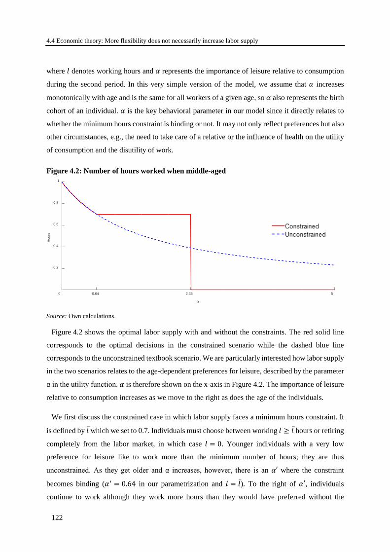
4.4 Economic theory: More flexibility does not necessarily increase labor supply
122
where 𝑙𝑙 denotes working hours and 𝛼𝛼 represents the importance of leisure relative to consumption
during the second period. In this very simple version of the model, we assume that 𝛼𝛼 increases
monotonically with age and is the same for all workers of a given age, so 𝛼𝛼 also represents the birth
cohort of an individual. 𝛼𝛼 is the key behavioral parameter in our model since it directly relates to
whether the minimum hours constraint is binding or not. It may not only reflect preferences but also
other circumstances, e.g., the need to take care of a relative or the influence of health on the utility
of consumption and the disutility of work.
Figure 4.2: Number of hours worked when middle-aged
Source: Own calculations.
Figure 4.2 shows the optimal labor supply with and without the constraints. The red solid line
corresponds to the optimal decisions in the constrained scenario while the dashed blue line
corresponds to the unconstrained textbook scenario. We are particularly interested how labor supply
in the two scenarios relates to the age-dependent preferences for leisure, described by the parameter
α in the utility function. 𝛼𝛼 is therefore shown on the x-axis in Figure 4.2. The importance of leisure
relative to consumption increases as we move to the right as does the age of the individuals.
We first discuss the constrained case in which labor supply faces a minimum hours constraint. It
is defined by 𝑙𝑙 ̅which we set to 0.7. Individuals must choose between working 𝑙𝑙 ≥ 𝑙𝑙 ̅hours or retiring
completely from the labor market, in which case 𝑙𝑙 = 0. Younger individuals with a very low
preference for leisure like to work more than the minimum number of hours; they are thus
unconstrained. As they get older and α increases, however, there is an 𝛼𝛼′ where the constraint
becomes binding (𝛼𝛼′ = 0.64 in our parametrization and 𝑙𝑙 = 𝑙𝑙)̅. To the right of 𝛼𝛼′, individuals
continue to work although they work more hours than they would have preferred without the
0 0.64 2.36 5
Hou
rs
0.2
0.4
0.6
0.8
1
Constrained
Unconstrained
4. Dangerous Flexibility – Retirement Reforms Reconsidered
123
constraint. Increasing age and thus 𝛼𝛼 even further, we reach an 𝛼𝛼′′ where labor supply changes
qualitatively (𝛼𝛼′′ = 2.36 in our parametrization). This corresponds to the retirement age. Beyond
this age, individuals have a sufficiently high preference for leisure, 𝛼𝛼 > 𝛼𝛼′′, to retire fully and thus
work fewer hours than they would have preferred without the constraint.
After a flexibility reform which removes the constraints, individuals will follow the path of labor
supply represented by the dashed blue line in Figure 4.2. Nothing changes for the youngest
individuals with a very low 𝛼𝛼 < 𝛼𝛼′. Moderate- 𝛼𝛼 individuals with 𝛼𝛼′ < 𝛼𝛼 < 𝛼𝛼′′, however, reduce
their labor supply to a more desirable level in the unconstrained scenario. This produces a negative
effect on hours worked while leaving labor force participation unchanged. The oldest individuals
with a high preference for leisure (𝛼𝛼 > 𝛼𝛼′′) increase their working hours to the desired level rather
than retire early. This creates a positive effect on hours worked and labor force participation.
Our model therefore predicts an unambiguously positive effect of a flexibility reform on labor
force participation but generates opposing effects on total labor supply. Whether the negative effect
on total labor supply of those younger than the former mandatory retirement age dominates the
positive effect on total labor supply of those older than the former mandatory retirement age
depends on the distribution of 𝛼𝛼 representing the age-dependent preferences for leisure and thus the
size of the underlying birth cohorts.41 A flexibility reform put into place when the baby boomers
are still relatively young is therefore most likely to reduce total labor supply.
4.4.2 Model extensions and pension policy
The point of the preceding section was to show that even in a very simple model of labor supply
more flexibility does not necessarily mean more labor volume, using the combination of a
mandatory retirement age and a minimum hours constraint as an example for inflexibility.
In a richer model, there will be additional effects. Moreover, pension policies may shift the cut-
off point 𝛼𝛼′′ in Figure 4.2. This section provides examples which show that the basic insights of the
simple model are robust.
First, we may want to loosen the strict link between age and the preference for leisure and
introduce heterogeneity of preference within a given birth cohort. The simple model of Section 4.4.1
41 Age, as pointed out, also represents birth cohorts, and we interpret the model as if it were based on a stationary population.

4.4 Economic theory: More flexibility does not necessarily increase labor supply
124
can then be re-interpreted by replacing the single representative individual for each birth cohort by
the median individual. The mandatory retirement age becomes binding for all individuals who reach
this age and (still) have a lower preference for leisure than the median individual. Success and
failure of a flexibility reform does not only depend on the relative size of birth cohorts but also on
the distribution of leisure preferences within each cohort. Increasing flexibility means more labor
supply for individuals with a high preference for consumption while it means less labor supply for
individuals with a high preference for leisure.
Second, there may be repercussions of the constraints on labor supply at younger ages. We
therefore expand our simple model to a three period model (young, retirement window and old).
Individuals work during the first two periods. The retirement decision is taken in the second period.
All individuals are retired in the third period. They supply 𝑙𝑙1 and 𝑙𝑙2 hours of labor and receive an
hourly wage of 𝑤𝑤 in return. The remaining hours are dedicated to leisure. For convenience, the total
number of hours in a period is normalized to 1 (𝑙𝑙𝑡𝑡 < 1 for 𝑝𝑝 = 1,2,3).
The individuals’ period utility increases in consumption (𝑐𝑐𝑡𝑡) and leisure (1 − 𝑙𝑙𝑡𝑡) and is given by
the same additively separable utility function as in our simple model:
𝑒𝑒𝑡𝑡 = ln(𝑐𝑐𝑡𝑡) + 𝛼𝛼 ln (1 − 𝑙𝑙𝑡𝑡)
Individuals choose a sequence {𝑐𝑐𝑡𝑡 , 𝑙𝑙𝑡𝑡 , 𝑝𝑝 = 1 … 3} to maximize their lifetime utility, 𝑈𝑈, where:
𝑈𝑈 = �𝑒𝑒𝑡𝑡
3
𝑡𝑡=1
subject to the lifetime budget constraint:
�𝑤𝑤3
𝑡𝑡=1
𝑙𝑙𝑡𝑡 = �𝑐𝑐𝑡𝑡
3
𝑡𝑡=1
where we set the price of the consumption good to one and the time preference and interest rates to
zero.42 In the third period all workers are retired, 𝑙𝑙3 = 0. Consumption in retirement is financed by
saving or an equivalent actuarial pension implicit in the budget constraint of our model.
42 We make these simplifying assumptions to ease exposition. Introducing impatience or positive interest rates would not qualitatively change our results. Note that saving or an equivalent actuarial pension cancel from the lifetime budget constraint.
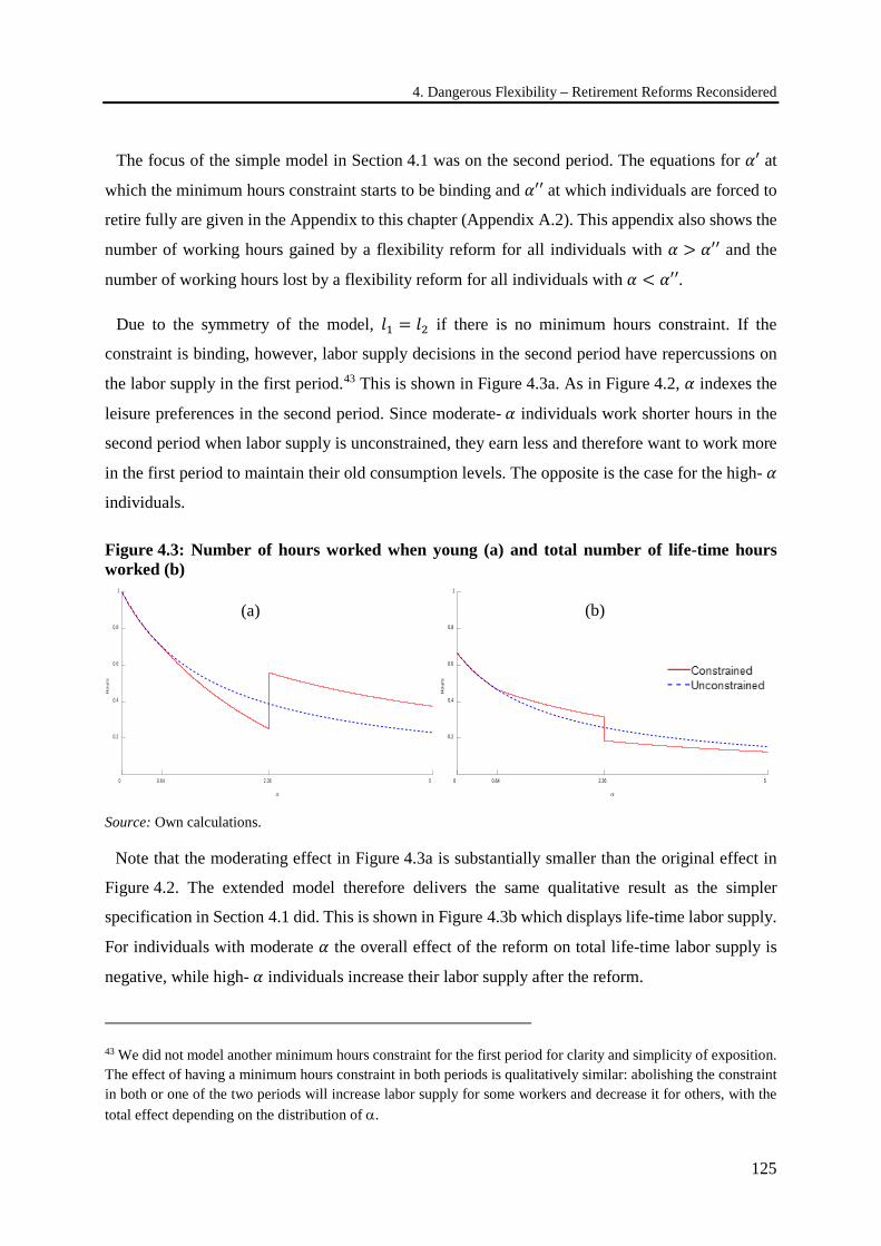
4. Dangerous Flexibility – Retirement Reforms Reconsidered
125
The focus of the simple model in Section 4.1 was on the second period. The equations for 𝛼𝛼′ at
which the minimum hours constraint starts to be binding and 𝛼𝛼′′ at which individuals are forced to
retire fully are given in the Appendix to this chapter (Appendix A.2). This appendix also shows the
number of working hours gained by a flexibility reform for all individuals with 𝛼𝛼 > 𝛼𝛼′′ and the
number of working hours lost by a flexibility reform for all individuals with 𝛼𝛼 < 𝛼𝛼′′.
Due to the symmetry of the model, 𝑙𝑙1 = 𝑙𝑙2 if there is no minimum hours constraint. If the
constraint is binding, however, labor supply decisions in the second period have repercussions on
the labor supply in the first period.43 This is shown in Figure 4.3a. As in Figure 4.2, 𝛼𝛼 indexes the
leisure preferences in the second period. Since moderate- 𝛼𝛼 individuals work shorter hours in the
second period when labor supply is unconstrained, they earn less and therefore want to work more
in the first period to maintain their old consumption levels. The opposite is the case for the high- 𝛼𝛼
individuals.
Figure 4.3: Number of hours worked when young (a) and total number of life-time hours worked (b)
Source: Own calculations.
Note that the moderating effect in Figure 4.3a is substantially smaller than the original effect in
Figure 4.2. The extended model therefore delivers the same qualitative result as the simpler
specification in Section 4.1 did. This is shown in Figure 4.3b which displays life-time labor supply.
For individuals with moderate 𝛼𝛼 the overall effect of the reform on total life-time labor supply is
negative, while high- 𝛼𝛼 individuals increase their labor supply after the reform.
43 We did not model another minimum hours constraint for the first period for clarity and simplicity of exposition. The effect of having a minimum hours constraint in both periods is qualitatively similar: abolishing the constraint in both or one of the two periods will increase labor supply for some workers and decrease it for others, with the total effect depending on the distribution of α.
0 0.64 2.36 5
Ho
urs
0.2
0.4
0.6
0.8
1
0 0.64 2.36 5
Ho
urs
0.2
0.4
0.6
0.8
1
Constrained
Unconstrained
(a) (b)
4.4 Economic theory: More flexibility does not necessarily increase labor supply
126
A third extension of our model involves pension policies. The separability of leisure and
consumption in the simple utility function implies that income changes affect consumption but not
the choice between work and leisure. In a technical sense, it makes life very easy because we can
ignore how pension income is provided. In a richer model, however, pension policies may shift the
cut-off point 𝛼𝛼′′ in Figure 4.2 and Figure 4.3. This mechanism explains how differences in leisure
preferences and pension policies across countries generate the different retirement patterns which
have been shown in Figure 4.1. We provide two examples:
Generosity of the pension system: As discussed in Section 4.2, the generosity of the pension
system especially in the years before the statutory retirement age crucially determines the retirement
decisions of workers. The more generous (early) pensions are, the higher the incentives to retire
early. This relationship has been extensively discussed in the literature and is supported by the
empirical evidence (see e.g. Gruber and Wise 2004).
To be precise, “generous” refers to an (early) retirement benefit that is larger than actuarially fair.
This is the case in most of the countries in our sample (Queisser and Whitehouse 2006, OECD
2015b). With a non-separable utility function, a higher income will increase consumption as well
as leisure, hence the cut-off point 𝛼𝛼′′ in Figure 4.2 and Figure 4.3 will shift to the left, increasing
the number of individuals who will retire fully when a minimum hours constraint is in place. Lifting
this constraint has therefore more likely a positive effect on total labor supply in an actuarially
unfair system which is generous to the early retirees relative to our baseline model. The total effect,
however, remains ambiguous.
Maximum hours constraints generated by earnings tests: In Section 4.2 we also discussed that
in many countries earnings tests limit the amount of labor income individuals can earn while
receiving a pension. In this sense, the earnings test is equivalent to a maximum hours constraint in
the second period. We discuss two cases. First, if the earnings limit is very low (see Table A.1.1),
the combination of minimum and maximum hours effectively prohibits work and forces individuals
to retire early even if their preferred hours were exceeding the minimum hours constraint. Making
the earnings test less incisive then unambiguously increases labor supply. Second, plugging a
maximum hours constraint into our model in 𝑝𝑝 = 2 reveals that, in this case, individuals would try
to compensate the earnings lost due to the constraint by increasing their labor supply in 𝑝𝑝 = 1.
Relaxing a maximum hours constraint in our framework would thus reduce the hours worked in
𝑝𝑝 = 1 and increase the hours worked in 𝑝𝑝 = 2. In our simple model, total labor supply thus remains
4. Dangerous Flexibility – Retirement Reforms Reconsidered
127
unchanged; in a more complex model with age-dependent preferences for leisure, the total effect is
likely to be negative since the preference for leisure is supposedly larger in older age.
Börsch-Supan et al. (2017) show that the combination of early retirement incentives and earnings
tests can create distinct patterns of labor force exit and pension claiming age. If earnings tests are
lifted (i.e. maximum hours constraints are abolished) in the presence of non-actuarial adjustment
factors, this can lead to very early pensions claiming. This means that an increase in labor force
participation happens at the cost of the pension system since individuals have an incentive to claim
their pension as early as possible and continue to work according to their leisure preferences.
It is possible to merge all these extensions into a single structural model of saving and retirement.
This has been done by Gustman and Steinmeier (1986, 2004) for the US institutional environment
and results in a very complex dynamic programming model that has to be solved numerically. The
authors show that if a minimum hours constraint is present, individuals will immediately move from
full-time work to full retirement. This is the same qualitative result as derived from our simple
model.
4.5 Empirical analysis
4.5.1 Methodology
The objective of our empirical analysis is to estimate the effect of the flexibility reforms described
in Section 4.3 on total labor supply. We first estimate the effects on labor force participation
(extensive margin), then the effect on total hours worked for those who participate in the labor
market (intensive margin) and finally the effect on total labor supply.
We employ two different estimation methods. The first method is a pooled Ordinary Least Squares
(OLS) regression which captures the reform effect by a dummy variable indicating that the reform
is in effect (Section 4.5.3). This method combines cross-sectional data on N countries and T time
periods to produce a dataset of NxT observations. In our analysis we combine time series data for
nine countries which adopted a flexibility reform in the past as described in Section 4.3. The
advantage of the pooled OLS method is that combining time series with cross sections yields larger
samples than using only cross sections or time series. We obtain an average effect of the flexibility
reforms over all countries and time periods. The disadvantage of pooled OLS is that the estimated
effects may have no causal interpretation if the reforms were driven by unobserved time varying

4.5 Empirical analysis
128
factors that are more complex than those captured by country-specific linear time trends and which
may also affect labor force participation and/or working hours.
We therefore use as a second method, known as the synthetic control method (SCM), which was
proposed by Abadie and Gardeazabal (2003) and extended in Abadie et al. (2010, 2015) for each
country individually (Section 4.5.4). This means that for each treated country we construct a
synthetic control from a weighted average of untreated countries. The synthetic control country
should approximate the treated country without the reform as closely as possible. We use a set of
(at that point in time) non-treated OECD countries for this purpose. The weights for the control
countries are set in such a way that the pre-reform trends in labor force participation and working
hours, respectively, match the treated countries. The treatment effect is then estimated by taking the
difference between the outcome variable (labor force participation or working hours) in the treated
country and in its synthetic counterpart after the reform – similar to a difference-in-difference
estimator, permitting us to evaluate the effects of the flexibility reforms at the country level.
Additionally, endogeneity stemming from omitted variable bias is treated by allowing the existence
of unobserved time-varying variables in the estimation. The synthetic control method also permits
evaluating the heterogeneity of the reforms by country given the differences in the country
circumstances and the reform specifics as described in Section 4.3. The synthetic control method,
however, requires long time series of the outcome and the control variables not only for the treated
but also for untreated countries. Hence data limitations tend to weaken the theoretical advantages
of the synthetic control method.
Since the advantages and disadvantages of the two different empirical approaches complement
each other, it is important to employ both methods – pooled OLS and SCM – in order to increase
the validity and robustness of our empirical findings. As we will see, both methods produce rather
similar results, giving us confidence in the obtained results.
4.5.2 Data
The empirical analyses require a large amount of data; especially the synthetic control method
requires time series data for at least ten years before a flexibility reform came into effect in order to
construct the synthetic control country. In particular time series data on working hours for older
workers are hard to obtain; they are only available for more recent years restricting our analysis
depending on the year of the reform.
4. Dangerous Flexibility – Retirement Reforms Reconsidered
129
Dependent variables. Our main dependent variables are labor force participation and working
hours for the age groups 55-64 and 65+.44 Annual time series data on labor force participation and
working hours are obtained from different sources: the OECD’s Employment database, Eurostat,
Eurofound, the International Labour Organization (ILO) and from several national statistical
agencies (Australian Bureau of Statistics, Statistics Canada, Statistics Finland, Statistics Japan,
Central Bureau of Statistics of Norway, Statistics Portugal, Statistics Sweden, UK Data Service, US
Bureau of Labor Statistics). In order to obtain the total labor supply, we multiply labor force
participation rates and working hours at the country and year level.
Control variables.45 The labor force participation rates and working hours of younger
workers at ages 25-54 are included in the estimations to capture country-specific labor market
trends over time. These data are obtained from the same sources as the dependent variables. We
additionally control for the statutory eligibility age at which a person becomes eligible for full
(state) pension benefits, and the earliest eligibility age, when early retirement (mostly with reduced
benefits) is possible. Those data are obtained from the Social Security Administration’s Social
Security Programs Throughout the World (1985-2014), OECD’s Pensions at a Glance (OECD
2011a, 2013b) and Duval (2003). Average years of total schooling are taken from Barro and Lee
(2013). GDP per capita and life expectancy at birth are obtained from the OECD (OECD 2016a,
OECD 2016b). Summary statistics for all variables are presented in Table A.3.1.
Treated countries. Our basic estimation sample includes nine countries: Australia, Austria,
Belgium, Denmark, Finland, France, Germany46, The Netherlands and Sweden. The periods
covered in the OLS estimation are: 1983-2013 for Australia, Belgium, Denmark, France and
Germany, 1989-2013 for Finland, 1990-2013 for Sweden and 1995-2013 for Austria and The
Netherlands, resulting in an unbalanced panel of 242 observations. Due to the unavailability of the
data on working hours for the age group 65+, Sweden is not part of this analysis. As a result, the
44 For the labor force participation and the working hours we follow the OECD definition. The labor force participation rate is defined as the ratio of the labor force to the working-age population, broken down by age group. Working hours are defined as average weekly working hours of people who are employed and work full-time or part-time. 45 For the construction of some of the synthetic control countries we also used the years of early retirement, i.e. the difference between the statutory and the earliest eligibility age. The data on schooling are available in five-year increments and therefore, converted to annual frequency by means of linear interpolation. 46 Annual data on the labor force at the OECD are averages of monthly estimates supplied by the German authorities. From 1991 onwards, data for unified Germany are available.
4.5 Empirical analysis
130
number of observations drops to 218 for the older age group. The treatment dummy is constructed
according to the reform year as indicated in Table A.1.1.
Control countries. In the synthetic control method potential comparison countries for each
treated country are the OECD member countries which have not adopted a flexibility reform during
the observation period. The set of comparison countries and the observation periods may differ for
each treated country since the reform years are different in each country. Additionally, the
availability of the time series determines the observation periods. More precisely, a comparison
country is included in the estimation if a sufficiently long time series of the outcome and the control
variables before the reform (usually around ten years) is available and it has stayed untreated for a
sufficiently long time period after the reform took place in the treated country (here around seven
years).47 We selected the control countries in such a way that the residuals of the pre-treatment
trends between the synthetic control country and the treated country are minimized while at the
same time the length of the pre-treatment time series is maximized. The set of a specific treated
country and the comparison countries constitutes a balanced panel.48 In Table A.5.1 we report the
time periods included before and after the reform by country. Table A.6.1 and Table A.6.2 show
the set of comparison countries included in the estimation for each treated country including the
weight of each comparison country in the synthetic control and the time periods covered in the
estimation.49
47 Some treated countries which had flexibility reforms rather late have also been included among the untreated countries for the construction of the synthetic control group of countries that were treated early (e.g., Belgium, Finland, The Netherlands, and Sweden). 48 More specifically, we started the selection of control countries by including all those potential control countries for which at least ten years of data on labor force participation or hours worked were available, respectively, before the flexibility reform in a specific treated country was introduced. If the pre-treatment trend for the resulting synthetic control did not closely match the corresponding trend for the treated country before the reform, we successively included more countries with shorter time series. The match in trend development was checked graphically and by minimizing the root mean square error (RMSE). The inclusion of additional countries automatically reduces the length of the pre-treatment time period because a balanced panel of treatment and control countries is needed for the estimation. Thus, the time period used in the estimation was determined by adding or removing countries (see Appendix A.5 for details). 49 As a robustness check we estimated all our results excluding Luxemburg from the control group, since Luxemburg is a very small country with very close labor market ties to Germany, France and Belgium. Our results are robust to this change. Results are available upon request.
4. Dangerous Flexibility – Retirement Reforms Reconsidered
131
4.5.3 Pooled OLS
In the following, we first run pooled Ordinary Least Squares (OLS) regressions of labor force
participation and working hours. We estimate the following Equation 4.1 separately for men aged
55-64 and 65+ where these two age ranges roughly correspond to the age bands to the right and left
of 𝛼𝛼′′ in our theoretical model:
𝑌𝑌𝑖𝑖𝑡𝑡 = 𝛽𝛽0 𝐸𝐸𝑃𝑃𝑆𝑆𝐼𝐼𝑅𝑅𝐸𝐸𝐿𝐿𝑃𝑃𝑅𝑅𝑃𝑃𝑖𝑖𝑡𝑡 + 𝛽𝛽1𝐼𝐼𝑖𝑖𝑡𝑡 + 𝛿𝛿𝑖𝑖 + 𝑓𝑓(𝑝𝑝) + 𝑒𝑒𝑖𝑖𝑡𝑡 (4.1)
where 𝑌𝑌𝑖𝑖𝑡𝑡 is the dependent variable. It is alternatively labor force participation (LFP), working hours
(WH), or the multiplication of the two, i.e., total labor supply (TLS). i and t are country and time
suffices. 𝐸𝐸𝑃𝑃𝑆𝑆𝐼𝐼𝑅𝑅𝐸𝐸𝐿𝐿𝑃𝑃𝑅𝑅𝑃𝑃𝑖𝑖𝑡𝑡 is a dummy variable which is equal to one in the year of the reform and
in the subsequent years of the reform and is equal to zero otherwise.50 𝛿𝛿𝑖𝑖 is a set of country fixed
effects. 𝑒𝑒𝑖𝑖𝑡𝑡 is the error term. 𝐼𝐼𝑖𝑖𝑡𝑡 is a set of control variables including the labor force participation,
the hours worked or total labor supply of the young (25 to 54 year olds) depending on the
specification and the statutory and early pension eligibility ages in order to capture the generosity
of the pension systems. 𝑓𝑓(𝑝𝑝) specifies country-specific time trends or time fixed effects.
Table 4.1 shows the main explanatory variable of interest, the post-reform dummy for three
different specifications. The baseline specification has neither country-specific time trends nor time
fixed effects. The second specification includes a country-specific linear time trend while the third
specification includes time fixed effects. For all specifications we calculate standard errors which
are clustered at the country level (in round parentheses) and standard errors which are calculated
using the method developed by Driscoll and Kraay (1998) in order to account for serial and spatial
correlation (in square brackets). Significance levels are reported for both types of standard errors.
Note that accounting for serial and spatial correlation produces much sharper results.
50 Since France abolished flexible retirement in 2004, the reform dummy is set to zero thereafter.
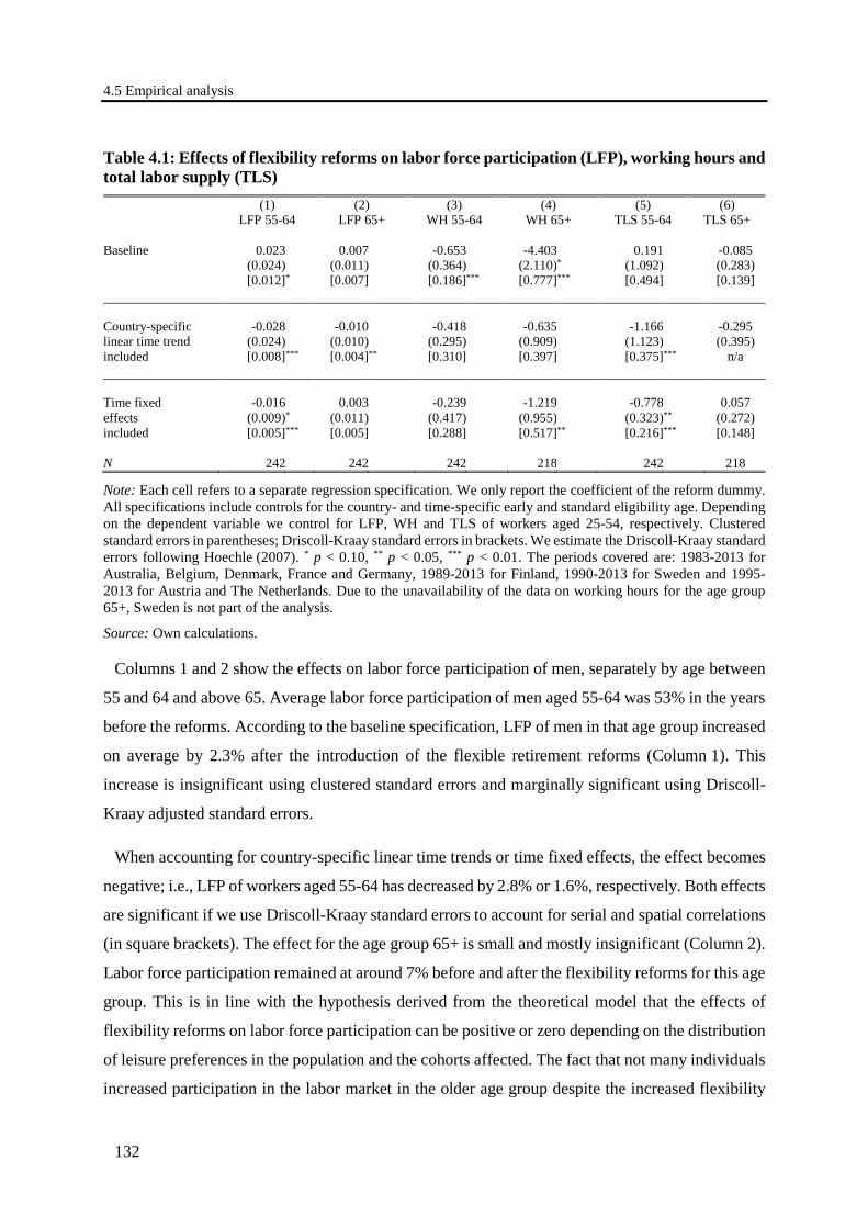
4.5 Empirical analysis
132
Table 4.1: Effects of flexibility reforms on labor force participation (LFP), working hours and total labor supply (TLS) (1)
LFP 55-64 (2)
LFP 65+ (3)
WH 55-64 (4)
WH 65+ (5)
TLS 55-64 (6)
TLS 65+ Baseline 0.023 0.007 -0.653 -4.403 0.191 -0.085 (0.024) (0.011) (0.364) (2.110) * (1.092) (0.283)
[0.012] * [0.007] [0.186] *** [0.777] *** [0.494] [0.139] Country-specific -0.028 -0.010 -0.418 -0.635 -1.166 -0.295 linear time trend (0.024) (0.010) (0.295) (0.909) (1.123) (0.395) included [0.008] *** [0.004] ** [0.310] [0.397] [0.375] *** n/a Time fixed -0.016 0.003 -0.239 -1.219 -0.778 0.057 effects (0.009) * (0.011) (0.417) (0.955) (0.323) ** (0.272) included [0.005] *** [0.005] [0.288] [0.517] ** [0.216] *** [0.148] N 242 242 242 218 242 218
Note: Each cell refers to a separate regression specification. We only report the coefficient of the reform dummy. All specifications include controls for the country- and time-specific early and standard eligibility age. Depending on the dependent variable we control for LFP, WH and TLS of workers aged 25-54, respectively. Clustered standard errors in parentheses; Driscoll-Kraay standard errors in brackets. We estimate the Driscoll-Kraay standard errors following Hoechle (2007). * p < 0.10, ** p < 0.05, *** p < 0.01. The periods covered are: 1983-2013 for Australia, Belgium, Denmark, France and Germany, 1989-2013 for Finland, 1990-2013 for Sweden and 1995-2013 for Austria and The Netherlands. Due to the unavailability of the data on working hours for the age group 65+, Sweden is not part of the analysis.
Source: Own calculations.
Columns 1 and 2 show the effects on labor force participation of men, separately by age between
55 and 64 and above 65. Average labor force participation of men aged 55-64 was 53% in the years
before the reforms. According to the baseline specification, LFP of men in that age group increased
on average by 2.3% after the introduction of the flexible retirement reforms (Column 1). This
increase is insignificant using clustered standard errors and marginally significant using Driscoll-
Kraay adjusted standard errors.
When accounting for country-specific linear time trends or time fixed effects, the effect becomes
negative; i.e., LFP of workers aged 55-64 has decreased by 2.8% or 1.6%, respectively. Both effects
are significant if we use Driscoll-Kraay standard errors to account for serial and spatial correlations
(in square brackets). The effect for the age group 65+ is small and mostly insignificant (Column 2).
Labor force participation remained at around 7% before and after the flexibility reforms for this age
group. This is in line with the hypothesis derived from the theoretical model that the effects of
flexibility reforms on labor force participation can be positive or zero depending on the distribution
of leisure preferences in the population and the cohorts affected. The fact that not many individuals
increased participation in the labor market in the older age group despite the increased flexibility
4. Dangerous Flexibility – Retirement Reforms Reconsidered
133
reflects their lower preferences for leisure. Our empirical results based on the OLS regressions give
a first indication that not even the effect of flexibility reforms on LFP is positive.
The effect of the reform on working hours of older workers is shown in Columns 3 and 4. Our
evidence here indicates that the average effect is negative both for workers before and after the
statutory eligibility age. The effects are significant in the baseline specification and for Driscoll-
Kraay adjusted standard errors. Most other specifications show insignificant effects.
We are ultimately interested in the overall effect of the flexibility reforms on total labor supply.
We therefore multiply the LFP and WH variables in order to obtain an unconditional measure of
the total labor supply and run the regressions with the same explanatory variables as before. Results
are presented in Columns 5 and 6. The effect on total labor force participation is not significant in
the baseline specification for both age groups. When we include country-specific linear time trends
or time fixed effects and use Driscoll-Kraay standard errors, then the overall effect on total labor
supply becomes significantly negative for workers aged 55-64 and remains insignificant for the
older age group.
In addition to the change in levels we checked how the flexibility reforms affected the trends in
labor force participation, hours worked and total labor supply (see Table A.4.1). Again we find that
flexibility reforms had largely negative effects on the labor markets in the countries under
consideration. On average labor force participation of male workers above age 55 increased, but the
increase was dampened by the flexibility reforms. The reforms also amplified the decrease in
weekly working hours. Overall, the yearly increase in total labor supply was dampened by 0.3%
due to the flexibility reforms.
In summary, the reforms did not produce the desired positive effect on total labor supply among
older male workers. On the contrary, both labor force participation and hours worked were affected
negatively by the flexibility reforms such that the overall effects were zero or negative in the nine
flexibility reforms included in our analysis.51
51 As results in Austria (see discussion in Section 4.5.4) might be confounded by the pension reform in 2004, we ran a robustness check dropping Austria and our general results remain.
4.5 Empirical analysis
134
4.5.4 Synthetic control method
4.5.4.1 The model
While we included country-specific linear time trends and common time fixed effects in the pooled
OLS estimations, the effects of the flexibility reforms may have been confounded by time trends
that have been more complex, e.g. non-linear with shapes that differed across countries. In this case,
the OLS results cannot be interpreted causally. Another disadvantage of the OLS method is that we
pooled reforms across countries and time and thus obtain an average measure of the effects of the
reforms described in Section 4.3. These reforms were, however, quite heterogeneous. We therefore
also pursue a second estimation strategy and apply the synthetic control method to those countries
that introduced a flexibility reform in the past. The model that we adopt is the following:
Let 𝐷𝐷𝑗𝑗𝑡𝑡 be an indicator for treatment, for country 𝑗𝑗 at time 𝑝𝑝. In our case this would be the adoption
of a flexibility reform. Then the observed outcome variable 𝑌𝑌𝑗𝑗𝑡𝑡 can be defined as the sum of a time-
varying treatment effect 𝛼𝛼𝑗𝑗𝑡𝑡𝐷𝐷𝑗𝑗𝑡𝑡 and the outcome that would have been observed for country 𝑗𝑗 at time
𝑝𝑝 if the reform had not taken place, expressed as 𝑌𝑌𝑗𝑗𝑡𝑡𝑁𝑁 (i.e. the counterfactual):
𝑌𝑌𝑗𝑗𝑡𝑡 = 𝛼𝛼𝑗𝑗𝑡𝑡𝐷𝐷𝑗𝑗𝑡𝑡 + 𝑌𝑌𝑗𝑗𝑡𝑡𝑁𝑁 = 𝛼𝛼𝑗𝑗𝑡𝑡𝐷𝐷𝑗𝑗𝑡𝑡 + (𝛿𝛿𝑡𝑡 + 𝜽𝜽𝒕𝒕𝒁𝒁𝒋𝒋 + 𝝀𝝀𝒕𝒕𝝁𝝁𝒋𝒋 + 𝜀𝜀𝑗𝑗𝑡𝑡) (4.2)
𝑌𝑌𝑗𝑗𝑡𝑡𝑁𝑁 is determined by 𝛿𝛿𝑡𝑡, an unknown time factor; 𝒁𝒁𝒋𝒋, a vector of observed covariates (not affected
by the treatment) which can be either time-invariant or time-varying; 𝜽𝜽𝒕𝒕, a vector of unknown
parameters; 𝝀𝝀𝒕𝒕, a vector of unobserved common factors; 𝝁𝝁𝒋𝒋, a vector of unknown factor loadings
and the error terms 𝜀𝜀𝑗𝑗𝑡𝑡 which are unobserved transitory shocks at the country level with zero mean.
Assuming that only the first country is exposed to the treatment, the treatment effect 𝐷𝐷𝑗𝑗𝑡𝑡 is estimated
by approximating the counterfactual 𝑌𝑌1𝑡𝑡𝑁𝑁 with a weighted average of untreated countries:
𝛼𝛼1𝑡𝑡� = 𝑌𝑌1𝑡𝑡 − ∑ 𝑤𝑤𝑗𝑗𝑌𝑌𝑗𝑗𝑡𝑡𝐽𝐽+1𝑗𝑗≥2 (4.3)
for 𝑝𝑝 ∈ {𝐼𝐼0 + 1, … ,𝐼𝐼} with 0 ≤ 𝑤𝑤𝑗𝑗 ≤ 1 for 𝑗𝑗 = 2, … , 𝐽𝐽 + 1 and 𝑤𝑤2 + ⋯+ 𝑤𝑤𝐽𝐽+1 = 1, 𝐼𝐼0 + 1 is the
year of the treatment, 𝐼𝐼 is the total number of years and 𝐽𝐽 + 1 is the total number of countries in the
sample. The weights are chosen such that pre-treatment characteristics of the treated country closely
reflect those of the synthetic control country. These characteristics include all those salient
covariates that explain the outcome variable and the pre-treatment values of the outcome variable.
4. Dangerous Flexibility – Retirement Reforms Reconsidered
135
Note that Equation 4.2 is equivalent to estimating a traditional fixed effect model if 𝜆𝜆𝑡𝑡𝑒𝑒𝑗𝑗 = 𝜙𝜙𝑗𝑗.
That is, the traditional fixed effect model assumes that unobserved heterogeneity is time-invariant.
The advantage of the synthetic control method over the fixed effect estimation is that it deals with
endogeneity stemming from omitted variable bias by allowing the existence of unobserved time-
varying variables in the estimation. Moreover, this method also allows for the presence of a common
time trend across countries.
4.5.4.2 Treatment effects
The quality of the estimation depends crucially on finding a good synthetic control. The synthetic
control must provide a good approximation how the outcome variable of the treated country would
have developed in the absence of the flexibility reform. This is the case if the counterfactual pre-
treatment values of the outcome variable provided by the synthetic control are close to the
corresponding values of the treated country. For constructing the synthetic control we use the
averages of the pre-treatment values of the outcome variables and a set of covariates which explain
the outcome variable. These covariates are labor force participation at younger ages 25-54, the
statutory eligibility age or the eligibility age for early retirement, GDP per capita, years of schooling,
and life expectancy (see Appendix to Chapter 4, Table A.8.1 and Table A.8.2, for the quality of pre-
treatment characteristics).52 Since alternative specifications are possible we report robustness
checks in Appendix A.7. We were unable to establish the robustness of the treatment effects on
labor force participation for Finland and The Netherlands, and on working hours for Sweden and
The Netherlands (see Figure A.7.1 and Figure A.7.2 in Appendix A.7). Therefore, we exclude those
countries when reporting the treatment effects in the rest of the chapter.
52 We do not include all lagged outcome values as predictors in order to increase the quality of the pre-treatment match since Kaul et al. (2015) show that the inclusion of the entire pre-treatment path of the outcome variable saturates the regression model and causes all other covariates to be irrelevant in the estimation. Note also, that the control variables in the SCM are not identical to the controls of the pooled OLS. In OLS we pool countries and years. We therefore run into multicollinearity problems if we include too many variables that only vary by country or only over time. In SCM, however, we are interested in getting a very good prediction of the pre-treatment trend in the outcome variable, so we include all variables that contribute to an improvement in fit even if they are highly correlated. In general, the criterion for selecting the inclusion of control countries and control variables was to minimize the RMSE.
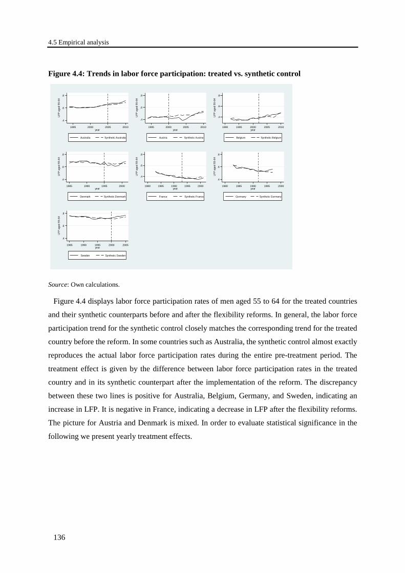
4.5 Empirical analysis
136
Figure 4.4: Trends in labor force participation: treated vs. synthetic control
Source: Own calculations.
Figure 4.4 displays labor force participation rates of men aged 55 to 64 for the treated countries
and their synthetic counterparts before and after the flexibility reforms. In general, the labor force
participation trend for the synthetic control closely matches the corresponding trend for the treated
country before the reform. In some countries such as Australia, the synthetic control almost exactly
reproduces the actual labor force participation rates during the entire pre-treatment period. The
treatment effect is given by the difference between labor force participation rates in the treated
country and in its synthetic counterpart after the implementation of the reform. The discrepancy
between these two lines is positive for Australia, Belgium, Germany, and Sweden, indicating an
increase in LFP. It is negative in France, indicating a decrease in LFP after the flexibility reforms.
The picture for Austria and Denmark is mixed. In order to evaluate statistical significance in the
following we present yearly treatment effects.
.4
.6
.8
LFP
aged
55-
64
1995 2000 2005 2010year
Australia Synthetic Australia
.4
.6
.8
LFP
aged
55-
64
1995 2000 2005 2010year
Austria Synthetic Austria
.4
.6
.8
LFP
aged
55-
64
1990 1995 2000 2005 2010year
Belgium Synthetic Belgium
.4
.6
.8
LFP
aged
55-
64
1985 1990 1995 2000year
Denmark Synthetic Denmark
.4
.6
.8
LFP
aged
55-
64
1980 1985 1990 1995 2000year
France Synthetic France
.4
.6
.8
LFP
aged
55-
64
1980 1985 1990 1995 2000year
Germany Synthetic Germany
.4
.6
.8
LFP
aged
55-
64
1985 1990 1995 2000 2005year
Sweden Synthetic Sweden
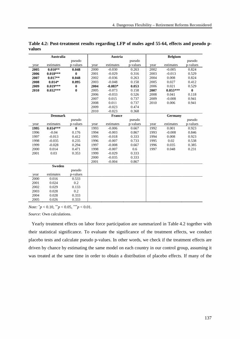
4. Dangerous Flexibility – Retirement Reforms Reconsidered
137
Table 4.2: Post-treatment results regarding LFP of males aged 55-64, effects and pseudo p-values
Australia Austria Belgium
year estimates pseudo
p-values year estimates pseudo
p-values year estimates pseudo
p-values 2005 0.010** 0.048 2000 -0.030 0.263 2002 -0.005 0.824 2006 0.018*** 0 2001 -0.029 0.316 2003 -0.013 0.529 2007 0.017** 0.048 2002 -0.036 0.263 2004 0.008 0.824 2008 0.014* 0.095 2003 -0.048 0.158 2005 0.027 0.412 2009 0.019*** 0 2004 -0.083* 0.053 2006 0.021 0.529 2010 0.032*** 0 2005 -0.073 0.158 2007 0.055*** 0
2006 -0.033 0.526 2008 0.041 0.118 2007 0.015 0.737 2009 -0.008 0.941 2008 0.011 0.737 2010 0.006 0.941 2009 -0.023 0.474 2010 -0.023 0.368
Denmark France Germany
year estimates pseudo
p-values year estimates pseudo
p-values year estimates pseudo
p-values 1995 0.034*** 0 1993 -0.006 0.667 1992 0.001 0.923 1996 -0.04 0.176 1994 -0.003 0.867 1993 -0.008 0.846 1997 -0.013 0.412 1995 -0.018 0.333 1994 0.008 0.923 1998 -0.035 0.235 1996 -0.007 0.733 1995 0.02 0.538 1999 -0.028 0.294 1997 -0.008 0.667 1996 0.035 0.385 2000 0.014 0.471 1998 -0.007 0.6 1997 0.048 0.231 2001 0.03 0.353 1999 -0.029 0.333
2000 -0.035 0.333 2001 -0.004 0.867
Sweden
year estimates pseudo
p-values 2000 0.016 0.533 2001 0.024 0.2 2002 0.029 0.133 2003 0.028 0.2 2004 0.028 0.333 2005 0.026 0.333
Note: *p < 0.10, **p < 0.05, ***p < 0.01.
Source: Own calculations.
Yearly treatment effects on labor force participation are summarized in Table 4.2 together with
their statistical significance. To evaluate the significance of the treatment effects, we conduct
placebo tests and calculate pseudo p-values. In other words, we check if the treatment effects are
driven by chance by estimating the same model on each country in our control group, assuming it
was treated at the same time in order to obtain a distribution of placebo effects. If many of the
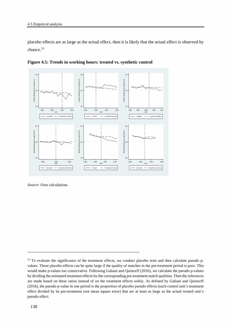
4.5 Empirical analysis
138
placebo effects are as large as the actual effect, then it is likely that the actual effect is observed by
chance.53
Figure 4.5: Trends in working hours: treated vs. synthetic control
Source: Own calculations.
53 To evaluate the significance of the treatment effects, we conduct placebo tests and then calculate pseudo p-values. Those placebo effects can be quite large if the quality of matches in the pre-treatment period is poor. This would make p-values too conservative. Following Galiani and Quistorff (2016), we calculate the pseudo p-values by dividing the estimated treatment effects by the corresponding pre-treatment match qualities. Then the inferences are made based on these ratios instead of on the treatment effects solely. As defined by Galiani and Quistorff (2016), the pseudo p-value in one period is the proportion of placebo pseudo effects (each control unit’s treatment effect divided by its pre-treatment root mean square error) that are at least as large as the actual treated unit’s pseudo effect.
30
40
50
Wee
kly W
orki
ng H
ours
age
d 55
-64
1995 2000 2005 2010year
Australia Synthetic Australia
30
40
50
Wee
kly W
orki
ng H
ours
age
d 55
-64
1995 2000 2005 2010year
Austria Synthetic Austria
30
40
50
Wee
kly W
orki
ng H
ours
age
d 55
-64
1990 1995 2000 2005 2010year
Belgium Synthetic Belgium
30
40
50
Wee
kly W
orki
ng H
ours
age
d 55
-64
1990 1995 2000year
Denmark Synthetic Denmark
30
40
50
Wee
kly W
orki
ng H
ours
age
d 55
-64
1985 1990 1995 2000year
France Synthetic France
30
40
50W
eekly
Wor
king
Hou
rs a
ged
55-6
4
1985 1990 1995 2000year
Germany Synthetic Germany

4. Dangerous Flexibility – Retirement Reforms Reconsidered
139
The results in Table 4.2 suggest that the estimated effect of the reform on labor force participation
is close to zero in most of the post-reform years in most of the countries. It is positive and
statistically significant only for Australia in all years after the reform. For Belgium there is a
significant increase in labor force participation only in 2007, five years after the introduction of the
reform. For Denmark the labor force participation significantly increased in the year of the reform
only. For France, Germany, and Sweden the reform did not change the labor force participation
significantly. Only for Austria we observe a weakly significant negative effect on labor force
participation in 2004, four years after the reform was enacted. Thus, with the exception of Australia,
there does not seem to be a consistent pattern of increased labor force participation due to the
flexibility reforms.
In Figure 4.5 we show the trends in weekly working hours for men aged 55 to 64 for the treated
countries and their synthetic counterparts. In general, pre-treatment observation periods for working
hours are shorter compared to pre-treatment observation periods for labor force participation due to
data restrictions. Nevertheless, the synthetic control matches for actual pre-treatment working hours
were stable for six of our initial countries. Robustness checks are shown in the Appendix to this
Chapter 4 (Figure A.7.2).
According to Figure 4.5, the estimated effects of the flexibility reforms on working hours are
negative in Australia, Belgium, France and Germany. The hours worked increased in Austria and
the picture is mixed for the post-treatment years in Denmark.
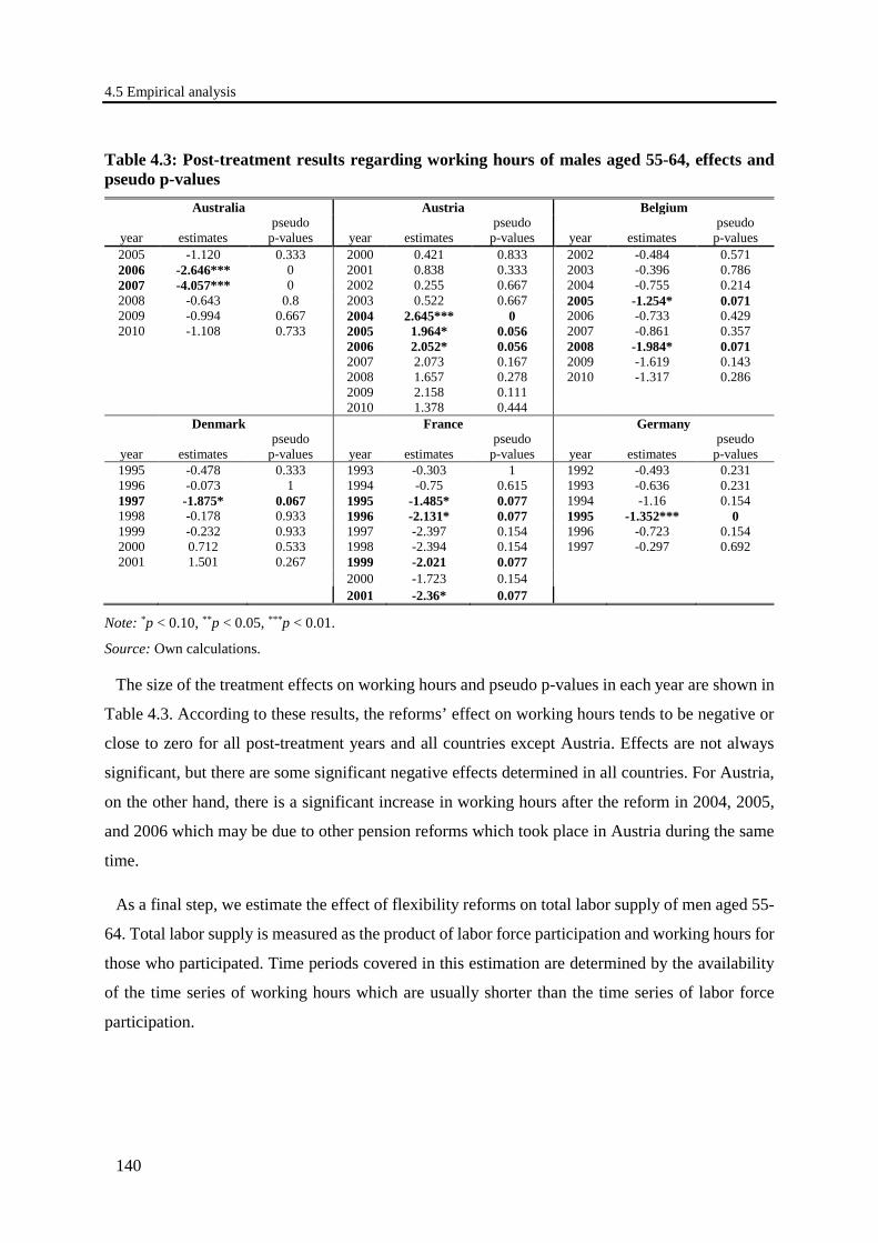
4.5 Empirical analysis
140
Table 4.3: Post-treatment results regarding working hours of males aged 55-64, effects and pseudo p-values
Australia Austria Belgium
year estimates pseudo
p-values year estimates pseudo
p-values year estimates pseudo
p-values 2005 -1.120 0.333 2000 0.421 0.833 2002 -0.484 0.571 2006 -2.646*** 0 2001 0.838 0.333 2003 -0.396 0.786 2007 -4.057*** 0 2002 0.255 0.667 2004 -0.755 0.214 2008 -0.643 0.8 2003 0.522 0.667 2005 -1.254* 0.071 2009 -0.994 0.667 2004 2.645*** 0 2006 -0.733 0.429 2010 -1.108 0.733 2005 1.964* 0.056 2007 -0.861 0.357
2006 2.052* 0.056 2008 -1.984* 0.071 2007 2.073 0.167 2009 -1.619 0.143 2008 1.657 0.278 2010 -1.317 0.286 2009 2.158 0.111 2010 1.378 0.444
Denmark France Germany
year estimates pseudo
p-values year estimates pseudo
p-values year estimates pseudo
p-values 1995 -0.478 0.333 1993 -0.303 1 1992 -0.493 0.231 1996 -0.073 1 1994 -0.75 0.615 1993 -0.636 0.231 1997 -1.875* 0.067 1995 -1.485* 0.077 1994 -1.16 0.154 1998 -0.178 0.933 1996 -2.131* 0.077 1995 -1.352*** 0 1999 -0.232 0.933 1997 -2.397 0.154 1996 -0.723 0.154 2000 0.712 0.533 1998 -2.394 0.154 1997 -0.297 0.692 2001 1.501 0.267 1999 -2.021 0.077
2000 -1.723 0.154 2001 -2.36* 0.077
Note: *p < 0.10, **p < 0.05, ***p < 0.01.
Source: Own calculations.
The size of the treatment effects on working hours and pseudo p-values in each year are shown in
Table 4.3. According to these results, the reforms’ effect on working hours tends to be negative or
close to zero for all post-treatment years and all countries except Austria. Effects are not always
significant, but there are some significant negative effects determined in all countries. For Austria,
on the other hand, there is a significant increase in working hours after the reform in 2004, 2005,
and 2006 which may be due to other pension reforms which took place in Austria during the same
time.
As a final step, we estimate the effect of flexibility reforms on total labor supply of men aged 55-
64. Total labor supply is measured as the product of labor force participation and working hours for
those who participated. Time periods covered in this estimation are determined by the availability
of the time series of working hours which are usually shorter than the time series of labor force
participation.
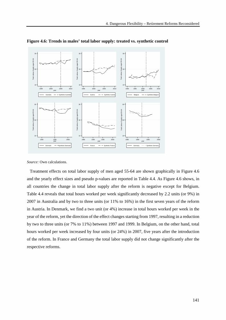
4. Dangerous Flexibility – Retirement Reforms Reconsidered
141
Figure 4.6: Trends in males’ total labor supply: treated vs. synthetic control
Source: Own calculations.
Treatment effects on total labor supply of men aged 55-64 are shown graphically in Figure 4.6
and the yearly effect sizes and pseudo p-values are reported in Table 4.4. As Figure 4.6 shows, in
all countries the change in total labor supply after the reform is negative except for Belgium.
Table 4.4 reveals that total hours worked per week significantly decreased by 2.2 units (or 9%) in
2007 in Australia and by two to three units (or 11% to 16%) in the first seven years of the reform
in Austria. In Denmark, we find a two unit (or 4%) increase in total hours worked per week in the
year of the reform, yet the direction of the effect changes starting from 1997, resulting in a reduction
by two to three units (or 7% to 11%) between 1997 and 1999. In Belgium, on the other hand, total
hours worked per week increased by four units (or 24%) in 2007, five years after the introduction
of the reform. In France and Germany the total labor supply did not change significantly after the
respective reforms.
10
20
30
Tota
l Lab
our S
uppl
y ag
ed 5
5-64
1995 2000 2005 2010year
Australia Synthetic Australia
10
20
30
Tota
l Lab
our S
uppl
y ag
ed 5
5-64
1995 2000 2005 2010year
Austria Synthetic Austria
10
20
30
Tota
l Lab
our S
uppl
y ag
ed 5
5-64
1990 1995 2000 2005 2010year
Belgium Synthetic Belgium
10
20
30
Tota
l Lab
our S
uppl
y ag
ed 5
5-64
1990 1995 2000year
Denmark Synthetic Denmark
10
20
30
Tota
l Lab
our S
uppl
y ag
ed 5
5-64
1985 1990 1995 2000year
France Synthetic France
10
20
30
Tota
l Lab
our S
uppl
y ag
ed 5
5-64
1985 1990 1995 2000year
Germany Synthetic Germany
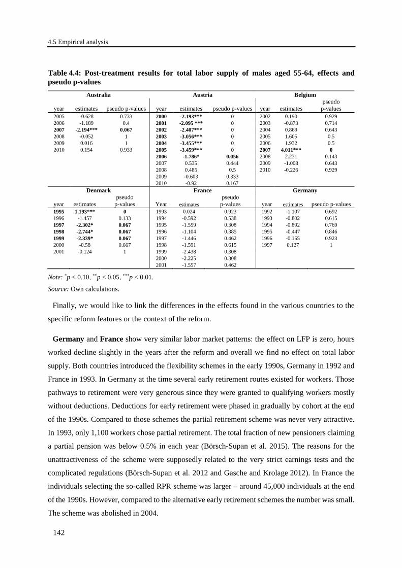
4.5 Empirical analysis
142
Table 4.4: Post-treatment results for total labor supply of males aged 55-64, effects and pseudo p-values
Australia Austria Belgium
year estimates pseudo p-values year estimates pseudo p-values year estimates pseudo
p-values 2005 -0.628 0.733 2000 -2.193*** 0 2002 0.190 0.929 2006 -1.189 0.4 2001 -2.095 *** 0 2003 -0.873 0.714 2007 -2.194*** 0.067 2002 -2.407*** 0 2004 0.869 0.643 2008 -0.052 1 2003 -3.056*** 0 2005 1.605 0.5 2009 0.016 1 2004 -3.455*** 0 2006 1.932 0.5 2010 0.154 0.933 2005 -3.459*** 0 2007 4.011*** 0
2006 -1.786* 0.056 2008 2.231 0.143 2007 0.535 0.444 2009 -1.008 0.643 2008 0.485 0.5 2010 -0.226 0.929 2009 -0.603 0.333 2010 -0.92 0.167
Denmark France Germany
year estimates pseudo
p-values Year estimates pseudo
p-values year estimates pseudo p-values 1995 1.193*** 0 1993 0.024 0.923 1992 -1.107 0.692 1996 -1.457 0.133 1994 -0.592 0.538 1993 -0.802 0.615 1997 -2.302* 0.067 1995 -1.559 0.308 1994 -0.892 0.769 1998 -2.744* 0.067 1996 -1.104 0.385 1995 -0.447 0.846 1999 -2.339* 0.067 1997 -1.446 0.462 1996 -0.155 0.923 2000 -0.58 0.667 1998 -1.591 0.615 1997 0.127 1 2001 -0.124 1 1999 -2.438 0.308
2000 -2.225 0.308 2001 -1.557 0.462
Note: *p < 0.10, **p < 0.05, ***p < 0.01.
Source: Own calculations.
Finally, we would like to link the differences in the effects found in the various countries to the
specific reform features or the context of the reform.
Germany and France show very similar labor market patterns: the effect on LFP is zero, hours
worked decline slightly in the years after the reform and overall we find no effect on total labor
supply. Both countries introduced the flexibility schemes in the early 1990s, Germany in 1992 and
France in 1993. In Germany at the time several early retirement routes existed for workers. Those
pathways to retirement were very generous since they were granted to qualifying workers mostly
without deductions. Deductions for early retirement were phased in gradually by cohort at the end
of the 1990s. Compared to those schemes the partial retirement scheme was never very attractive.
In 1993, only 1,100 workers chose partial retirement. The total fraction of new pensioners claiming
a partial pension was below 0.5% in each year (Börsch-Supan et al. 2015). The reasons for the
unattractiveness of the scheme were supposedly related to the very strict earnings tests and the
complicated regulations (Börsch-Supan et al. 2012 and Gasche and Krolage 2012). In France the
individuals selecting the so-called RPR scheme was larger – around 45,000 individuals at the end
of the 1990s. However, compared to the alternative early retirement schemes the number was small.
The scheme was abolished in 2004.
4. Dangerous Flexibility – Retirement Reforms Reconsidered
143
Denmark enacted the flexibility reform in 1995. We find a positive LFP effect in the first year
after the reform, and a negative effect on WH after three years. Overall, total labor supply increased
only in the first year of the reform and after that decreased slightly. Hansen (2001) reports that the
Danish part-time scheme never attracted many participants (only around 1,000 per year). He
proposes that this could be due to the unavailability of suitable part-time jobs. Additionally, an
attractive early retirement scheme existed in Denmark which attracted around 150,000 individuals
at the end of the 1990s (Hansen 2001). Thus, similar to France and Germany the partial retirement
scheme in Denmark seemed to lack popularity most likely due to the simultaneous existence of
attractive routes for full early retirement.
Austria adopted the part-time scheme in 2000. We find no effect on LFP except in 2004, where
we find a negative effect, which is contrary to our predictions, but only weakly significant at the
10% level. We find a positive effect on weekly working hours in the years 2004 to 2006 which is
again in contrast to all other countries in our study. It is strongly significant for the year 2004 in
which the flexibility scheme was reformed again. What we see is most likely not the effect of the
flexibility reform in 2000 but rather the effect of the pension reform in 2004. This reform made
early retirement more costly by increasing eligibility ages to various early retirement pathways and
introducing actuarial adjustments to benefits received before the statutory retirement age. Overall,
however, we find a significantly negative effect of the flexibility reforms on total labor supply.
These results are in line with the micro-econometric estimation results obtained by Graf et al. (2008,
2011) who find a significant reduction of the part-time scheme on total labor supply for both men
and women.
The Belgian part-time scheme was introduced in 2002, after the baby-boomers had already started
to retire. We find zero effects on LFP in all years except in 2007, where we find a significantly
positive effect on LFP. Effects on working hours are mostly negative, however they are only
significant in 2005 and 2008. The effect of the flexibility scheme on total labor supply is zero in all
years except in 2007. Here the positive effect on LFP creates an overall positive effect on labor
supply. Overall, the time credit scheme is evaluated as successful scheme in terms of take-up. It
was criticized because it did not show the desired effects of keeping individuals in the labor force
longer, but it was used in some sectors as an early exit scheme (Albanese et al. 2015).
Australia enacted the reform in 2005, when the baby-boomers had already started to retire (the
oldest baby-boomer cohort reached the retirement window in 2001). It is the only country where
we find a consistently positive effect of the reform on LFP. However, we find a slightly negative

4.6 Conclusions
144
effect on working hours after two and three years, so that the overall effect of the reform on labor
supply becomes zero (negative in year three after the reform). Overall, only few relatively wealthy
workers opted for the scheme. This could be related to the tax incentives or lack of information
about the available options (Australian Government 2015).
In summary, we find that labor force participation slightly increased or stayed the same in most
countries after the introduction of the flexibility reforms. At the same time hours worked largely
decreased after the reforms. The overall effects on total labor supply are either zero or negative,
except for Belgium, where we find a slight increase in total labor supply five years after the
flexibility reform.
Results from the pooled OLS and SCM approaches thus consistently point into the same
directions. This makes us confident that the evidence is robust in spite of the various caveats of the
methods and the dearth of data available especially for working hours in the early periods of our
investigation.
4.6 Conclusions
Making retirement more flexible sounds like a good thing for sure. If the aim is to increase labor
supply at older ages, however, this is not necessarily true. From a theoretical point of view,
flexibility reforms have ambiguous effects on labor supply and might endanger the intended goal
of increasing total labor volume. Our empirical analyses show that they have actually done so in
most of the countries in our study.
Total labor supply is the product of labor force participation (the extensive margin) and average
hours worked (the intensive margin). One has to consider the effects of increased flexibility on both
margins. Our theoretical model shows that the effect of a reform on labor force participation is
positive if workers value leisure highly. If they have a moderate or low preference for leisure, there
will be no effect on labor force participation. Moreover, the effect on total hours worked can be
positive or negative depending on the distribution of age-related leisure preferences in the
population.
We exploit the evidence drawn from several flexibility reforms that were introduced in nine
OECD countries between 1992 and 2006. Using two different econometric approaches, we reach
the same conclusion: labor force participation has very little if at all increased in some countries
and years due to the flexibility reforms introduced since the 1990s. At the same time we find that
4. Dangerous Flexibility – Retirement Reforms Reconsidered
145
older men aged 55-64 have decreased their weekly working hours. In sum, the reforms have
produced zero to negative effects on total labor supply. Hence, if the objective of these flexibility
reforms was to increase labor supply of older workers, they have failed to reach this aim.
Notwithstanding this failure, flexibility reforms are a good thing for the targeted workers when
they remove constraints such that individuals are put into a situation which permits them to better
trade-off leisure and consumption in their specific life circumstances. For instance, if individuals
would like to spend time caring for a relative, retire jointly with a spouse, or are not healthy enough
to work full time but would like to work part-time and smooth consumption, more flexible
retirement conditions are likely to increase the utility of the targeted individuals. This is where the
intuition of “more flexibility is better” holds.
Whether welfare for society as a whole increases is another issue. If more flexibility comes along
with lower total labor supply and higher pension expenditures, then the tax and contribution base
will be reduced and taxes and pension contributions will have to be increased. This will lessen the
utility of tax payers and younger workers. The tax and contribution increases will be particularly
strong in pension systems in which benefits are not linked in an actuarially neutral way to the
retirement age. Whether overall societal welfare increases or decreases then depends on the
underlying demographic structure and the respective weights given to each cohort.
Welfare is also affected by general equilibrium effects. First, higher taxes and contributions will
have feedback effects on labor supply. Second, aggregate productivity might be affected depending
on the age structure of the workforce and the number of full-time and part-time workers. Moreover,
fixed costs of part-time work and frictions related to this have to be taken into account. The analysis
of welfare effects therefore requires a macro-economic model with multiple generations and strong
assumptions how to aggregate the utility functions of each cohort, see e.g. Börsch-Supan et
al. (2016). Due to the different mechanisms and trade-offs, it is ex ante unclear whether the net
effect of more flexibility on welfare for society as a whole is positive or negative.
The message of this study is therefore that increasing flexibility has two sides: a potentially
positive side for the targeted older workers and a dangerous one for an aging society as a whole.
Flexibility may taste sweet but policy makers cannot escape the fact that if one wants to increase
labor volume for an aging population, one must increase the average exit age from the labor force.
The danger of flexibility reforms is the suggestion that such an escape is possible.

4.6 Conclusions
146
How can one sweeten this sour fruit? Increasing the retirement age has often been perceived as
exchanging years in sweet retirement for years in sour work. This view is wrong since during the
period in which the retirement age will be gradually increased, life expectancy will also increase –
short of an unlikely reversal of the trend during the last decades. This permits increasing the length
of the working life in parallel to increasing the length of life in retirement. Stabilizing the financial
base of a pension system with respect to ever longer lives only requires stabilizing the ratio of time
spent in retirement to time spent in work. Thus, to make it concrete, the sour fruit of 2 years more
work can be sweetened by 1 year more retirement made possible by an increase of life expectancy
by 3 years. These numbers correspond to the ratio of roughly 40 years of work and 20 years of
retirement in most OECD countries, plus the fact that these countries gain about 3 years of life
expectancy in about 15 calendar years if the trend of the last decades will continue. Even better
would be to make this proportionality rule an automatic stabilizer as proposed by Börsch-Supan
(2007) and OECD (2011b) which could then also accommodate different speeds or even a reversal
in the increase of life expectancy.
Other possible accompanying measures are the abolishment of all earnings tests – if, and this is a
strong if, pension systems are made actuarially fair. Earnings tests are only necessary if the pension
system provides non-actuarial transfers. In a DC system in which benefits match contributions,
earnings tests are superfluous (Disney and Smith 2002).
Mandatory retirement ages are obviously counterproductive to flexibility and longer working
lives. The often voiced argument that older workers need to make place for the young is wrong, at
least in such generality, see the country studies in Gruber and Wise (2010). As we have shown,
minimum hours constraints imposed by employers have effects similar to a mandatory retirement
age. In a modern service economy, fixed costs of work are probably much lower than they were in
economies dominated by manufacturing, hence such constraints could be abolished.
In a package with all these elements, flexibility reforms are a complement, not a substitute. While
the evidence is still outstanding, such a package is more likely to increase total labor volume and
thereby strengthen the financial base of our pension systems.
147
5. Dangerous Flexible Retirement Reforms – A Supplementary Placebo Analysis across Time
This chapter is single-authored.
5.1 Introduction
Declining birth rates paired with an increase in life expectancy lead to population aging in many
countries around the world. These developments together with the looming retirement of the baby
boomers put enormous pressure on pension systems within the next years. To ease the burden of
these developments, a common aim of governments in many developed countries has been to
strengthen the pool of older workers. However, increasing eligibility ages for drawing pension
benefits as one option of keeping older workers in the labor market is not a very popular policy.
Therefore, many governments have enacted flexible retirement options that allow workers to
gradually reduce work effort with increasing age. The aim of those reforms is to provide a seemingly
elegant way to increase older workers’ labor supply.
From a theoretical point of view, however, the model of a stylized flexibility reform in Chapter 4
of this dissertation shows that flexibility reforms can have ambiguous effects on total labor supply.
While flexibilization is likely to increase labor force participation among older workers, it may
decrease their working hours. Consequently, the effect on total labor supply is ex ante unclear and
remains an empirical question. The analysis in Chapter 4, therefore, evaluates flexibility reforms
from different OECD countries enacted between 1992 and 2006 and finds that they produced zero
to negative effects on total labor supply. The conclusion is that flexibility reforms can be regarded
as dangerous instruments for two reasons: First, if the aim was to increase older worker’s labor
5.1 Introduction
148
supply these reforms have failed to reach their objective. Second, the reforms may have additionally
postponed or even replaced the introduction of more effective policies.
In Chapter 4, the synthetic control method – proposed by Abadie and Gardeazabal (2003) and
extended in Abadie et al. (2010, 2015) – is applied to study the effects of different flexibility
reforms. Aim of Chapter 4 is to investigate the effect of flexibility reforms on the labor force
participation rate (extensive margin), the average number of weekly working hours (intensive
margin), and on the total labor volume of men aged 55-64. The latter is the product of intensive and
extensive margin. According to Athey and Imbens (2017), the synthetic control method “is
arguably the most important innovation in the policy evaluation literature in the last 15 years”. It
builds on the idea of difference-in-differences estimations which have been an important tool for
empirical research since the early 1990s (see, for instance, the classic difference-in-differences
study by Card 1990). The advantage of the synthetic control method lies in the acknowledgement
of the premise that, when the unit(s) of interest are only a few aggregate entities, such as countries,
states, regions, or cities, a combination of comparison units (called “synthetic control group”)
usually better reproduces the characteristics of the unit(s) of interest than any single comparison
unit alone. Hence, the idea of the synthetic control method consists in constructing the synthetic
control group as a weighted average of all potential comparison units that best resembles the pre-
treatment characteristics of the case of interest (Abadie et al. 2015). The post-treatment outcomes
of the treated unit are then compared to the post-treatment outcomes of the untreated synthetic
control group. With that, it becomes possible to estimate what would have happened to the treated
unit of interest in the absence of a specific treatment or intervention (such as, e.g., event, shock,
law, reform).
Abadie et al. (2010) state that the potential applicability of the synthetic control method to
comparative case studies is very large since many policy interventions or other events of interest
take place at an aggregate level (e.g., countries, states, regions, cities) and affect only a small
number of aggregate units. This holds especially in situations where traditional regression methods
are not appropriate. In line with this prediction, the synthetic control method has been applied across
various fields over the last years.
As Abadie et al. (2010) further note, large sample inference techniques are, however, problematic
for comparative case studies when the number of comparison units is small. Already in Abadie and
Gardeazabal (2003), the authors therefore proposed placebo studies to perform inference when
applying the synthetic control method. The basic idea of placebo studies is to reassign the treatment

5. Dangerous Flexible Retirement Reforms – A Supplementary Placebo Analysis across Time
149
to members of the control group that were not actually exposed to it. Abadie et al. (2015) refer to
this procedure as “in-space placebos”. If many of the placebo effects are as large as the actual effect,
it is likely that the actual effect is observed by mere chance. An alternative dimension that can be
used for placebo studies is the timing of the treatment: Instead of reassigning the treatment to
actually untreated countries, it can also be assigned to points in time when the intervention did not
occur. Abadie et al. (2010) refer to this exercise as “in-time placebos”.
To perform inference, Chapter 4 applies in-space placebos by reassigning the intervention (i.e. the
coming into force of a flexible retirement reform) to other members of the control group which did
not experience a reform in the same year. The research aim of this chapter is to investigate the same
reforms and to scrutinize the former results by making use of the time dimension in the placebo
studies. This is achieved by reassigning the flexibility reforms to dates when they did not actually
happen (i.e. in-time placebos). The rationale behind this exercise is the following: If I found
estimated effects in the analysis of reforms assigned to dates where they did not actually happen
that are of similar or larger magnitude than the effects estimated for the actual reform years in
Chapter 4, the confidence in these results would diminish. In this case, the estimated effects for the
actual flexibility reforms would hardly be attributable to these reforms. Put in the opposite way: It
increases the confidence of the results found in Chapter 4, if the application of the in-time placebo
studies does not yield significant effects.
The remainder of the chapter is as follows: Section 5.2 discusses the synthetic control method,
highlights requirements and limitations of the method and reviews the application of placebo studies
in the field of the synthetic control method in more detail. A description of the data used in this
chapter is given in Section 5.3. Section 5.4 presents the results from the in-time placebo study and
recalls the results of Chapter 4 to ease a direct comparison of all results. Section 5.5 summarizes
the findings and concludes that the results found in Chapter 4 are stable to the robustness check in
the form of the in-time placebo studies.
5.2 The synthetic control method
150
5.2 The synthetic control method
The synthetic control method is a data-driven approach to estimate treatment effects of policy
interventions in comparative case studies (Abadie and Gardeazabal 2003, Abadie et al. 2010, 2015).
Similar to a difference-in-differences design, the synthetic control method exploits the difference
in treated and untreated units across an event of interest. In the environment of Chapter 4 and this
chapter, the events of interest are the flexibility reforms in the respective OECD countries.
However, in contrast to a difference-in-differences approach, the synthetic control method does not
give the same weight to all untreated units. Instead, the procedure induces a weighted average of
the untreated units that closely matches the pretreatment-trend of the treated unit. Outcomes for this
synthetic control are then projected into the post-treatment period using the weights emerging from
the pre-treatment trend matching. This projection serves as a counterfactual for the treated unit
approximating the outcome that would have been observed in the treated country without the
intervention. In the following, the synthetic control model is described in more formal detail
following Abadie et al. (2010, 2015).
5.2.1 The model
The model supposes that there is a sample of 𝐽𝐽 + 1 units indexed by 𝑗𝑗 which will be countries in the
context of this chapter. Only the first country 𝑗𝑗 = 1 is exposed to the treatment or intervention of
interest. Here, the event of interest is the adaption of the flexibility reform. The remaining countries
𝑗𝑗 > 1 constitute the synthetic control group, a reservoir of comparison countries (in the usage of
Abadie and co-authors called “donor pool”).
Let 𝐷𝐷𝑗𝑗𝑡𝑡 further be an indicator that takes the value 1 if the treatment occurred for country 𝑗𝑗 at
time 𝑝𝑝. Then the observed outcome variable 𝑌𝑌𝑗𝑗𝑡𝑡 can be defined as the sum of a time-varying
treatment effect 𝛼𝛼𝑗𝑗𝑡𝑡𝐷𝐷𝑗𝑗𝑡𝑡 and the outcome that would have been observed for country 𝑗𝑗 at time 𝑝𝑝 if the
reform had not taken place. The latter is the counterfactual expressed as 𝑌𝑌𝑗𝑗𝑡𝑡𝑁𝑁 :
𝑌𝑌𝑗𝑗𝑡𝑡 = 𝛼𝛼𝑗𝑗𝑡𝑡𝐷𝐷𝑗𝑗𝑡𝑡 + 𝑌𝑌𝑗𝑗𝑡𝑡𝑁𝑁 (5.1)
5. Dangerous Flexible Retirement Reforms – A Supplementary Placebo Analysis across Time
151
Suppose that the counterfactual 𝑌𝑌𝑗𝑗𝑡𝑡𝑁𝑁 is given by
𝑌𝑌𝑗𝑗𝑡𝑡𝑁𝑁 = 𝛿𝛿𝑡𝑡 + 𝜽𝜽𝒕𝒕𝒁𝒁𝒋𝒋 + 𝝀𝝀𝒕𝒕𝝁𝝁𝒋𝒋 + 𝜀𝜀𝑗𝑗𝑡𝑡 (5.2)
where 𝛿𝛿𝑡𝑡 is an unknown time factor, 𝒁𝒁𝒋𝒋 a vector of observed covariates (not affected by the
treatment) which can be either time-invariant or time-varying, 𝜽𝜽𝒕𝒕 a vector of unknown parameters,
𝝀𝝀𝒕𝒕 a vector of unobserved common factors, 𝝁𝝁𝒋𝒋 a vector of unknown factor loadings and the error
terms 𝜀𝜀𝑗𝑗𝑡𝑡 which are unobserved transitory shocks at the country level with zero mean.
The treatment effect 𝑎𝑎𝑗𝑗𝑡𝑡 is estimated by approximating the counterfactual 𝑌𝑌1𝑡𝑡𝑁𝑁 with a weighted
combination of untreated countries:
𝑎𝑎�1𝑡𝑡 = 𝑌𝑌1𝑡𝑡 − ∑ 𝑤𝑤𝑗𝑗𝑌𝑌𝑗𝑗𝑡𝑡𝐽𝐽+1𝑗𝑗≥2 (5.3)
for 𝑝𝑝 ∈ {𝐼𝐼0 + 1, … ,𝐼𝐼}, with a (J × 1) vector of weights 𝑊𝑊 = (𝑤𝑤2, … ,𝑤𝑤𝐽𝐽+1)’ with 0 ≤ 𝑤𝑤𝑗𝑗 ≤ 1 for
𝑗𝑗 = 2, … , 𝐽𝐽 + 1 and 𝑤𝑤2 + ⋯+ 𝑤𝑤𝐽𝐽+1 = 1. 𝐼𝐼0 + 1 is the year of the treatment, and 𝐼𝐼 is the total
number of years. Note that choosing a specific value of 𝑊𝑊 is equivalent to choosing a particular
synthetic control.
The weights are chosen such that pre-treatment characteristics of the treated country are best
resembled by the characteristics of the synthetic control. More formally, suppose that 𝐼𝐼1 is a (k ×
1) vector with the values of the pre-treatment characteristics of the treated units which should be
matched as closely as possible, and let 𝐼𝐼0 be the (k × 1) vector collecting the same variables for
the units in a synthetic control group. Note that pre-treatments characteristics in 𝐼𝐼1 and 𝐼𝐼0 may
include pre-treatment values of the outcome variable. Consequently, the vector (𝐼𝐼1 − 𝐼𝐼0𝑊𝑊) gives
the difference between the pre-treatment characteristics of the treated unit and a synthetic control.
The weights, 𝑊𝑊*, are selected in a way which minimizes the distance
‖𝐼𝐼1 −𝐼𝐼0𝑊𝑊‖v = �(𝐼𝐼1 − 𝐼𝐼0𝑊𝑊)′𝑉𝑉(𝐼𝐼1 − 𝐼𝐼0𝑊𝑊) (5.4)
with 𝑉𝑉 is some (k × k) positive semidefinite matrix indicating the importance of each predictor.54
54 There are different techniques of obtaining 𝑉𝑉 (see Abadie et al. 2010). Following Abadie et al. 2010 and Abadie and Gardeazabal 2003, in the empirical section in this chapter the weights are chosen such that the root mean squared error (RMSE) of the outcome variable is minimized for the pre-treatment periods (see also Abadie and Gardeazabal 2003, Appendix B, for more details). This is the same approach as in Chapter 4.
5.2 The synthetic control method
152
Notice that Equation 5.1 and Equation 5.2 put together generalize a traditional fixed effect model
that is often applied in empirical studies. The traditional fixed effects model can be obtained when
imposing that 𝜆𝜆𝑡𝑡𝑒𝑒𝑗𝑗 = 𝜙𝜙𝑗𝑗 in Equation 5.2 by assuming that unobserved heterogeneity is time-
invariant. The advantage of the synthetic control method over the fixed effect estimation is that it
deals with endogeneity stemming from omitted variable bias as it allows unobserved variables in
the estimation that vary with time. Moreover, the synthetic control method allows for the presence
of a common time trend across countries as well.
After estimating the treatment effect, statistical significance can be determined by running placebo
tests and calculating pseudo p-values. Estimating the same model on each untreated unit of the
synthetic control yields a distribution of placebo effects. If many of the placebo effects are as large
as the actual effect, it is likely that the actual effect is observed by mere chance. Following Galiani
and Quistorff (2016), the pseudo p-value can be written as
𝑒𝑒 − 𝑐𝑐𝑎𝑎𝑙𝑙𝑒𝑒𝑎𝑎 =∑ 𝐼𝐼(│𝑎𝑎�𝑗𝑗𝑁𝑁│≥│𝑎𝑎�1𝑁𝑁│)𝐽𝐽+1𝑗𝑗≥2
𝐽𝐽 (5.5)
with 𝑝𝑝 as given above and 𝐼𝐼(│𝑎𝑎�𝑗𝑗𝑡𝑡│ ≥ │𝑎𝑎�1𝑡𝑡│) being an indicator that takes the value one if the
inequality in parentheses is fulfilled.55
5.2.2 Requirements and limitations of the synthetic control method
Constructing a synthetic control group requires a careful selection of comparison units: First, the
units in the control group should have similar characteristics as the treated unit to avoid interpolation
biases. To address this issue, both Chapter 4 and this chapter use OECD member countries as
potential comparison countries only. Moreover, units affected by the same or similar treatments, or
units that may have suffered large idiosyncratic shocks to the outcome variable should not be
included in the synthetic control group. In the sense of this chapter, this means that only those
OECD member countries, which have not adopted flexible retirement reforms during the
observation period, are potential comparison countries.
Key challenge of the synthetic control method is that it requires a substantial amount of data. This
in particular holds true for the number of pre-intervention periods. The reason is that the pre-
55 Following Galiani and Quistorff (2016), the pseudo p-values in the empirical section are adjusted with the pre-treatment match qualities. Otherwise, p-values could get too conservative. See Footnote 53 in Section 4.5.4 for more details.
5. Dangerous Flexible Retirement Reforms – A Supplementary Placebo Analysis across Time
153
treatment match of the synthetic control unit with the treated unit determines the credibility of the
synthetic control. Time series data in particular on working hours for older workers are, however,
hard to obtain. This especially holds true for data from before the turn of the millennium. Only in
recent years, data availability on working hours in the older age groups has increased. Abadie et
al. (2015) do not recommend applying the synthetic control method when the number of pre-
treatment periods is small unless the pre-treatment fit is good.56
5.2.3 Inference with the synthetic control method: in-space placebos and in-time
placebos
Abadie et al. (2015) recall that the use of statistical inference in comparative case studies is
problematic due to, for instance, the small-sample nature of the data or the absence of
randomization. These difficulties complicate traditional approaches to statistical inference. The
synthetic control method, however, allows conducting different falsification exercises akin to
permutation tests – termed placebo studies. The idea of these placebo studies is to artificially
reassign the intervention either to units that were not exposed to the treatment or to dates prior to
the actual intervention. The advantage of these inferential methods is that it can be used for both
individual (micro) and aggregate (macro) data, and can even be applied if the number of comparison
units in the synthetic control group is small (Abadie et al. 2010).
In their seminal paper on the economic effects of the terrorist conflict in the Basque Country,
Abadie and Gardeazabal (2003) already performed a placebo study to assess whether the terrorist
conflict truly had an effect on the economic performance or whether it was rather an artifact of a
poorly measured synthetic control. They find that after the outbreak of terrorism in the late 1960s
GDP per capita declined about ten percentage points compared to a synthetic control region without
terrorism. To assess whether the gap in GDP is actually driven by terrorism, they also applied the
method to a similar region (Catalonia in this case) which was not exposed to terrorism during the
observation period and compared the resulting estimates to the actual ones.
Abadie et al. (2010) extend the idea of placebo studies by applying the placebo treatments to every
comparison country in their control group. The authors study the effect of Proposition 99, a large-
scale tobacco control program which was implemented in California in 1988. They demonstrate
that tobacco consumption fell remarkably in California relative to a comparable synthetic control
56 Abadie et al. (2010) state that time series data for at least ten years before the treatment would be ideal.

5.2 The synthetic control method
154
region following Proposition 99. Their estimates suggest a decline of per-capita cigarette sales of
about 26 packs that can be attributed to Proposition 99. The control group in their study contains 38
US states that did not introduce formal statewide tobacco control programs or substantially raised
the states’ cigarette taxes during the observation period. To assess the significance of their estimates,
the authors conduct a series of placebo studies by iteratively applying the synthetic control method
to every other comparison state in the control group. They show that the estimated effect for
California during the study period 1989-2000 is unusually large relative to the distribution of the
effects for the states in the synthetic control.
In their most recent work, Abadie et al. (2015) apply the synthetic control method to the 1990
German reunification and investigate the economic impact on West Germany. Austria, the United
States, Japan, Switzerland, and The Netherlands constitute the control group. They find that
reunification had a negative effect on West German income, with a reduction of per-capita gross
domestic product (GDP) of about $1,600 per year on average over the 1990-2003 period. This
amounts to approximately 8% of the 1990 baseline level. To evaluate the credibility of their
estimates, they for one thing conduct in-space placebos by artificially reassigning the intervention
to each member of the control group. In addition, they apply in-time placebos by reassigning the
reform to dates when the actual intervention did not occur. As placebo reform year, they use 1975
instead of the actual reunification year 1990.57 The interpretation of this approach is similar to the
in-space placebo approach: If similarly large effects could be obtained when applying the treatment
to dates at which it did not occur, the confidence about the existence of an effect would dissipate.
They show that their results are robust across both placebo dimensions and a further sensitivity
check.58
The results of Chapter 4 are based on in-space placebos. In other words, it is under investigation
if the treatment effects of the flexibility reforms are driven by chance by estimating the same model
on each country in the synthetic control group, assuming it was treated at the same time. In doing
57 The authors show that their results are similar when reassigning the placebo reform year to 1970 and 1980, respectively. 58 Though sometimes described as “in-place” or “cross-sectional placebo tests” by other authors, the main methodology of in-space placebos remains the same. I follow the nomenclature of Abadie et al. (2015) regarding “in-space placebos” and “in-time placebos”, respectively, in the rest of the dissertation. Another sensitivity check proposed by Abadie et al. (2015) is reducing the number of units in the synthetic control to analyze whether the results are sensitive to single units in the synthetic control. The exclusion of Luxembourg later in this study represents such a further sensitivity check (see Section 5.4 and Appendix B.5).
5. Dangerous Flexible Retirement Reforms – A Supplementary Placebo Analysis across Time
155
so, we obtain a distribution of placebo effects against which we can evaluate the effect estimated
for the reform-treated country.
In contrast to the application of in-space placebos in Chapter 4, this chapter applies in-time
placebos by reassigning the flexibility reforms to placebo reform dates other than the actual reform
year. The placebo reform years are set three years earlier than the actual reform years. The choice
of three years is the same for all countries and is the result of a compromise: As historical time
series data, in particular on working hours for older age groups are hard to obtain, the choice of
three years still allows a pre-treatment period with some years. Simultaneously, the determination
of three years still ensures a post-placebo-treatment period consisting of three treatment effects until
the actual reform effect would influence the effects. Abadie et al. (2015) emphasize that the number
of post-treatment years should not be too small in case the treatment effect only emerges gradually
after the intervention.
Since Abadie and Gardeazabal (2003), numerous authors have utilized the synthetic control
method across many fields over the last years.59 Among the literature, it appears that in-space
placebos are the most widely used base to performing inference (Bilgel and Galle 2015, Bohn et al.
2014, Cavallo et al. 2013, Kleven et al. 2013, Liu 2015, Stearns 2015). A few papers utilize in-time
placebos to prove the validity of their estimates (Freire 2018, Saia 2017). However, in-time placebos
are clearly in the minority. While other authors have analyzed the effectiveness of the synthetic
control method using Monte Carlo simulations (see, e.g., Ferman et al. 2020, Hahn and Shi 2017,
Kaul et al. 2015, O’Neill et al 2016, Gobillon and Magnac 2016), it appears that the majority of
synthetic control literature focusses on choosing one placebo test, either in-space or in-time. This
chapter adds to the very few to date who compare both (see beside, Abadie et al. 2015).
59 For instance in Acemoglu et al. (2016) on political connections, Abadie et al. (2010) (tobacco control program), Abadie et al. (2015) (Germany’s reunification), Bilgel and Galle (2015) (organ donations), Bohn et al. (2014) (2007 Legal Arizona Workers Act), Cavallo et al. (2013) (natural disasters), Gobillon and Magnac (2016) (enterprise zones), Hinrichs (2012) (affirmative action bans on college enrolment), Kleven et al. (2013) (taxation of athletes), Kreif et al. (2016) and O’Neill (2016) (health improvement), Liu (2015) (spillover from universities), Nannicini and Billmeier (2011) and Billmeier and Nannicini (2013) (economic growth).
5.3 Data and variables
156
5.3 Data and variables
The empirical analysis with the synthetic control method requires a large amount of data. In
particular, the fact that time series data are not only necessary for the treated countries but also for
all control countries increases the required amount of data.60
Dependent variables. The main dependent variables are labor force participation (extensive
margin) and working hours (intensive margin) of males for the age groups 55-64. The outcome
variable total labor supply is obtained by multiplying labor force participation rates and working
hours at the country and year level. Annual time series data on labor force participation and working
hours are obtained from different sources: the OECD’s Employment database, Eurostat, Eurofound,
the International Labour Organization (ILO) and from several national statistical agencies
(Australian Bureau of Statistics, Statistics Canada, Statistics Finland, Statistics Japan, Central
Bureau of Statistics of Norway, Statistics Portugal, Statistics Sweden, UK Data Service, US Bureau
of Labor Statistics).
Control variables. From the same sources as the dependent variables, I use the labor force
participation rate and the average number of weekly working hours of the young (age group 25-54)
as control variables. These variables capture country-specific labor market trends over time.
Variables describing the pension system serve as control variables as well: these are the statutory
eligibility age at which workers become eligible for full pension benefits regardless of any other
qualification and the earliest eligibility age. The latter is defined as the age at which early retirement
is possible, mostly with reduced benefits.61 The data describing the pension system are obtained
from the Social Security Administration’s Social Security Programs throughout the World (1985-
2014), OECD’s Pensions at a Glance (OECD 2011a, 2013b) and Duval (2003). Data on years of
total schooling are from Barro and Lee (2013). GDP per capita and life expectancy at birth are taken
from the OECD’s database (OECD 2016a, OECD 2016b).
Treated countries and placebo reform years. The countries under investigation in this chapter
are the ones part of the empirical analysis with the synthetic control method in Chapter 4 to enable
a meaningful comparison, namely: Australia, Austria, Belgium, Denmark, France, Germany, and
60 The data used in this chapter are the same as in Chapter 4. 61 See the glossary of Börsch-Supan and Coile (2019).
5. Dangerous Flexible Retirement Reforms – A Supplementary Placebo Analysis across Time
157
Sweden.62 For the application of in-time placebo studies, the placebo reform years (PRY) are chosen
to be three years earlier compared to the years where the flexibility reforms actually were adapted.
This means: Australia: PRY=2002, Austria: PRY=1997, Belgium: PRY=1999, Denmark:
PRY=1992, France: PRY=1990, Germany: PRY=1989, and Sweden: PRY=1997.63
Control countries. The pool of potential comparison countries comprises the OECD member
countries that have not adopted a flexibility reform during the observation period of each country.64
The actual selection of comparison countries for the synthetic controls for the treated countries is
the same as in Chapter 4 and differs for each treated country since the (placebo) reform years are
different in each country. In addition, data availability determines observation periods. The data set
for each treated country and its comparison countries in this chapter constitute a balanced panel,
meaning a longitudinal data set where all units are observed at the same time periods. Table B.1.1
reports the time series included before and after the placebo reform year by country and by outcome
variable. Table B.2.1 and Table B.2.2 show the comparison countries, which constitute the synthetic
controls for each treated country, and present the weight of each comparison country in the control
group. The two tables in addition show the time periods included in the estimation.
62 The analysis in Chapter 4 started by additionally looking at flexibility reforms in Finland, The Netherlands, and Sweden. However, with the data at hand we were not able to find robust synthetic controls for Finland and The Netherlands for all outcome variables. Regarding Sweden, we only found a proper synthetic control for the outcome variable labor force participation, but not for the outcome variable weekly working hours. Therefore, the analysis on Sweden is restricted to labor force participation. 63 Table A.1.1 (Appendix A.1) comprises comprehensive details of the flexibility reforms. The table comprises country-specific information on gender-specific statutory eligibility ages for public pension, the age at which the flexible retirement window starts if flexible retirement schemes are available through systems other than the public pension scheme, information on the extent to which the working time must be reduced within the flexible retirement option, information on the income loss compensating financial sources, whether earnings tests apply, and mandatory retirement regulations. 64 Belgium and Sweden, which had flexibility reforms rather late, have also been included among the untreated countries for the construction of the synthetic control group of countries that were treated early.
5.4 Results
158
5.4 Results
Finding a good synthetic control country is crucial for the estimation quality. The synthetic country
should as closely as possible approximate how the outcome variable of the treated country would
have developed without the flexibility reform. This is the case if the synthetic control country
provides a counterfactual pre-treatment value of the outcome variable that comes close to the
corresponding value of the treated country.
The approach for constructing the synthetic control in this chapter is the same as in Chapter 4 to
allow a clear comparison: For the outcome variables, labor force participation of males aged 55-64
and working hours of males aged 55-64, I use the average of the pre-treatment values of the outcome
variables for constructing the synthetic control.65 In addition, I control for a set of covariates which
explain the outcome variables. These covariates are the labor force participation rate of the younger
age group (age 25-54) when the outcome variable is labor force participation, the number of
working hours of the younger age group (age 25-54) when the outcome variable is working hours,
the multiplication of extensive and intensive margin of the younger age group (age 25-54) when the
outcome variable is total labor volume, the statutory eligibility age or the earliest eligibility age.
Moreover, gross domestic product (GDP, per capita), years of schooling, and life expectancy are
control variables.66 Table B.4.1 and Table B.4.2 show the quality of pre-treatment characteristics
by comparing the pre-treatment characteristics of the treated country with that of the synthetic
control country. Total labor supply is measured as the product of labor force participation and
working hours for those who participated.
The application of the in-time placebo studies in this chapter reduces the number of pre-treatment
years because the placebo reforms years are reassigned to three years earlier that the actual reform
came into effect. However, even with the shorter pre-treatment periods, the estimation yields
65 Alternative specifications are, e.g., controlling for the last pre-treatment value of the outcome variable only or including all lagged outcome values as predictors. I report robustness checks in Appendix 3 comparing the different possible specifications (i.e. average pre-treatment value vs. last pre-treatment value vs. all pre-treatment values of labor force participation rate). Kaul et al. (2018), however, demonstrate both theoretically and empirically that controlling for all outcome lags causes all other covariates to be irrelevant. Therefore, I do not include all lagged outcome values as predictors. In general, the criterion for selecting the inclusion of control countries and control variables is to minimize the root mean squared error (RMSE). 66 For the construction of some of the synthetic control countries, I use the years of early retirement as control variable. This variable is measured as the difference between the statutory eligibility age and the earliest eligibility age. The data on schooling are available in five-year increments and, therefore, converted to annual frequency by means of linear interpolation.
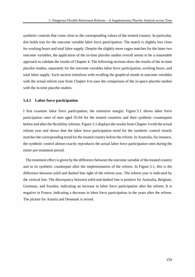
5. Dangerous Flexible Retirement Reforms – A Supplementary Placebo Analysis across Time
159
synthetic controls that come close to the corresponding values of the treated country. In particular,
this holds true for the outcome variable labor force participation. The match is slightly less close
for working hours and total labor supply. Despite the slightly more vague matches for the latter two
outcome variables, the application of the in-time placebo studies overall seems to be a reasonable
approach to validate the results of Chapter 4. The following sections show the results of the in-time
placebo studies, separately for the outcome variables labor force participation, working hours, and
total labor supply. Each section initializes with recalling the graphical trends in outcome variables
with the actual reform year from Chapter 4 to ease the comparison of the in-space placebo studies
with the in-time placebo studies.
5.4.1 Labor force participation
I first examine labor force participation, the extensive margin: Figure 5.1 shows labor force
participation rates of men aged 55-64 for the treated countries and their synthetic counterparts
before and after the flexibility reforms. Figure 5.1 displays the results from Chapter 4 with the actual
reform year and shows that the labor force participation trend for the synthetic control closely
matches the corresponding trend for the treated country before the reform. In Australia, for instance,
the synthetic control almost exactly reproduces the actual labor force participation rates during the
entire pre-treatment period.
The treatment effect is given by the difference between the outcome variable of the treated country
and in its synthetic counterpart after the implementation of the reform. In Figure 5.1, this is the
difference between solid and dashed line right of the reform year. The reform year is indicated by
the vertical line. The discrepancy between solid and dashed line is positive for Australia, Belgium,
Germany, and Sweden, indicating an increase in labor force participation after the reform. It is
negative in France, indicating a decrease in labor force participation in the years after the reform.
The picture for Austria and Denmark is mixed.
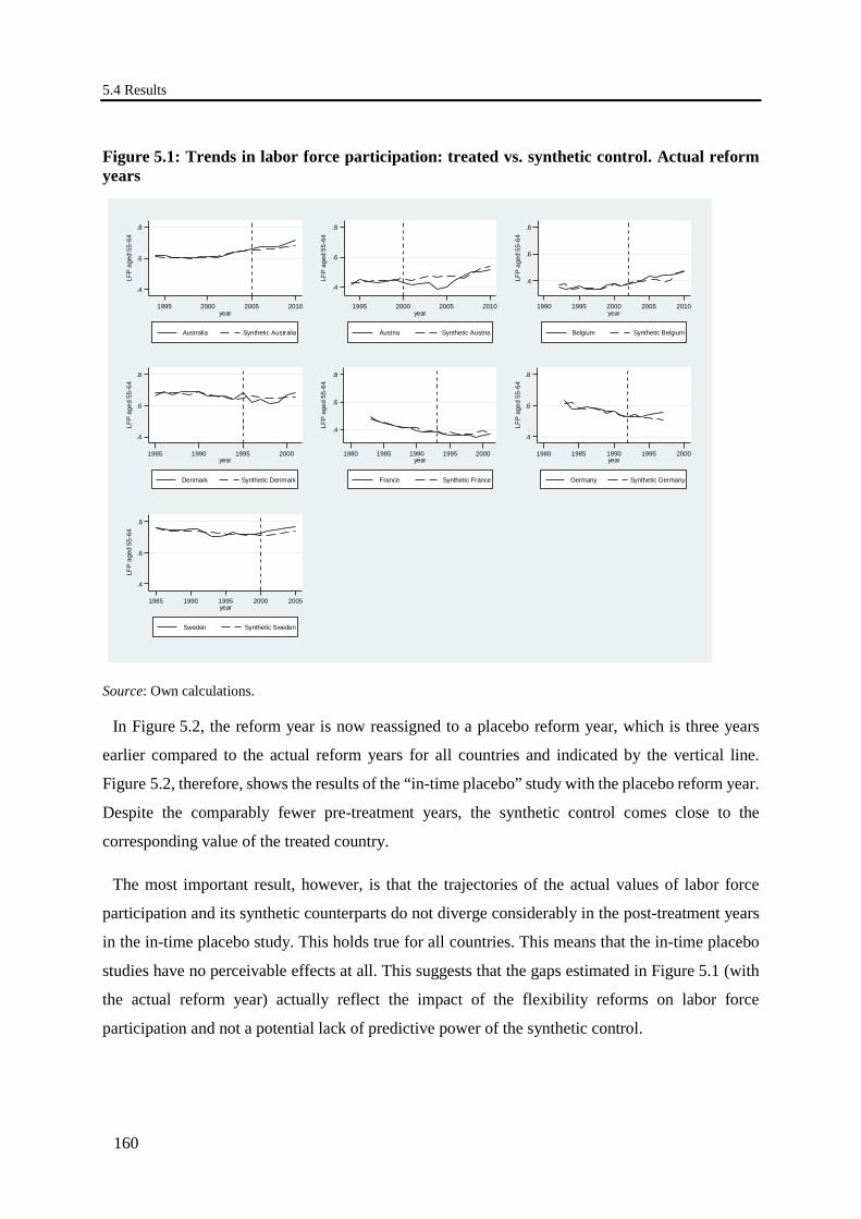
5.4 Results
160
Figure 5.1: Trends in labor force participation: treated vs. synthetic control. Actual reform years
Source: Own calculations.
In Figure 5.2, the reform year is now reassigned to a placebo reform year, which is three years
earlier compared to the actual reform years for all countries and indicated by the vertical line.
Figure 5.2, therefore, shows the results of the “in-time placebo” study with the placebo reform year.
Despite the comparably fewer pre-treatment years, the synthetic control comes close to the
corresponding value of the treated country.
The most important result, however, is that the trajectories of the actual values of labor force
participation and its synthetic counterparts do not diverge considerably in the post-treatment years
in the in-time placebo study. This holds true for all countries. This means that the in-time placebo
studies have no perceivable effects at all. This suggests that the gaps estimated in Figure 5.1 (with
the actual reform year) actually reflect the impact of the flexibility reforms on labor force
participation and not a potential lack of predictive power of the synthetic control.
.4
.6
.8
LFP
aged
55-
64
1995 2000 2005 2010year
Australia Synthetic Australia
.4
.6
.8
LFP
aged
55-
64
1995 2000 2005 2010year
Austria Synthetic Austria
.4
.6
.8
LFP
aged
55-
64
1990 1995 2000 2005 2010year
Belgium Synthetic Belgium
.4
.6
.8
LFP
aged
55-
64
1985 1990 1995 2000year
Denmark Synthetic Denmark
.4
.6
.8
LFP
aged
55-
64
1980 1985 1990 1995 2000year
France Synthetic France
.4
.6
.8
LFP
aged
55-
64
1980 1985 1990 1995 2000year
Germany Synthetic Germany
.4
.6
.8
LFP
aged
55-
64
1985 1990 1995 2000 2005year
Sweden Synthetic Sweden
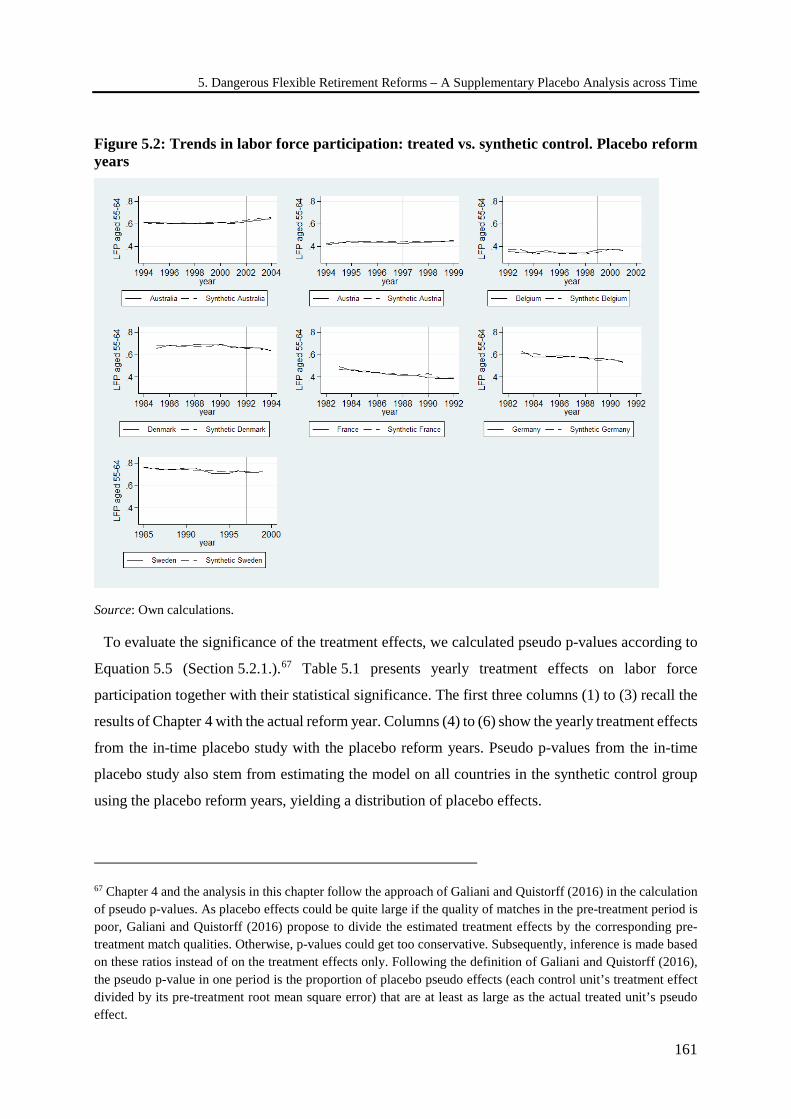
5. Dangerous Flexible Retirement Reforms – A Supplementary Placebo Analysis across Time
161
Figure 5.2: Trends in labor force participation: treated vs. synthetic control. Placebo reform years
Source: Own calculations.
To evaluate the significance of the treatment effects, we calculated pseudo p-values according to
Equation 5.5 (Section 5.2.1.).67 Table 5.1 presents yearly treatment effects on labor force
participation together with their statistical significance. The first three columns (1) to (3) recall the
results of Chapter 4 with the actual reform year. Columns (4) to (6) show the yearly treatment effects
from the in-time placebo study with the placebo reform years. Pseudo p-values from the in-time
placebo study also stem from estimating the model on all countries in the synthetic control group
using the placebo reform years, yielding a distribution of placebo effects.
67 Chapter 4 and the analysis in this chapter follow the approach of Galiani and Quistorff (2016) in the calculation of pseudo p-values. As placebo effects could be quite large if the quality of matches in the pre-treatment period is poor, Galiani and Quistorff (2016) propose to divide the estimated treatment effects by the corresponding pre-treatment match qualities. Otherwise, p-values could get too conservative. Subsequently, inference is made based on these ratios instead of on the treatment effects only. Following the definition of Galiani and Quistorff (2016), the pseudo p-value in one period is the proportion of placebo pseudo effects (each control unit’s treatment effect divided by its pre-treatment root mean square error) that are at least as large as the actual treated unit’s pseudo effect.
5.4 Results
162
Table 5.1 shows a first validation: While the results of Chapter 4 reveal significant results for
some countries, shifting the reform year suspends significance of effects. This is the case for almost
all countries in almost all years (except France in 1990). This means that in contrast to the actual
flexibility reforms, the placebo flexibility reforms have no perceivable effect.
Table 5.1: Post-treatment results regarding LFP of males aged 55-64, effects and pseudo p-values
“In-space placebos” (actual reform year, Chapter 4)
“In-time placebos” (placebo reform year)
(1) (2) (3) (4) (5) (6)
year estimates pseudo p-values year estimates pseudo p-values Australia
2002 -0.012 0.238 2003 -0.013 0.190 2004 -0.009 0.476
2005 0.010** 0.048 2005 2006 0.018*** 0 2006 2007 0.017** 0.048 2007 2008 0.014* 0.095 2008 2009 0.019*** 0 2009 2010 0.032*** 0 2010
Austria 1997 -0.016 0.421
1998 -0.004 1 1999 0.006 0.947
2000 -0.03 0.263 2001 -0.029 0.316 2002 -0.036 0.263 2003 -0.048 0.158 2004 -0.083* 0.053 2005 -0.073 0.158 2006 -0.033 0.526 2007 0.015 0.737 2008 0.011 0.737 2009 -0.023 0.474 2010 -0.023 0.368
Belgium 1999 0.021 0.235
2000 0.001 0.941 2001 0.002 0.882
2002 -0.005 0.824 2003 -0.013 0.529 2004 0.008 0.824 2005 0.027 0.412 2006 0.021 0.529 2007 0.055*** 0 2008 0.041 0.118 2009 -0.008 0.941 2010 0.006 0.941
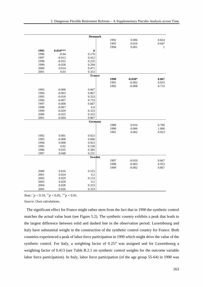
5. Dangerous Flexible Retirement Reforms – A Supplementary Placebo Analysis across Time
163
Denmark 1992 0.006 0.824
1993 0.010 0.647 1994 0.001 1
1995 0.034*** 0 1996 -0.04 0.176 1997 -0.013 0.412 1998 -0.035 0.235 1999 -0.028 0.294 2000 0.014 0.471 2001 0.03 0.353
France 1990 -0.038* 0.067
1991 -0.002 0.933 1992 -0.008 0.733
1993 -0.006 0.667 1994 -0.003 0.867 1995 -0.018 0.333 1996 -0.007 0.733 1997 -0.008 0.667 1998 -0.007 0.6 1999 -0.029 0.333 2000 -0.035 0.333 2001 -0.004 0.867
Germany 1989 0.016 0.769
1990 0.000 1.000 1991 0.002 0.923
1992 0.001 0.923 1993 -0.008 0.846 1994 0.008 0.923 1995 0.02 0.538 1996 0.035 0.385 1997 0.048 0.231
Sweden 1997 -0.010 0.667
1998 -0.003 0.933 1999 -0.002 0.867
2000 0.016 0.533 2001 0.024 0.2 2002 0.029 0.133 2003 0.028 0.2 2004 0.028 0.333 2005 0.026 0.333
Note: *p < 0.10, **p < 0.05, ***p < 0.01.
Source: Own calculations.
The significant effect for France might rather stem from the fact that in 1990 the synthetic control
matches the actual value least (see Figure 5.2). The synthetic country exhibits a peak that leads to
the largest difference between solid and dashed line in the observation period. Luxembourg and
Italy have substantial weight in the construction of the synthetic control country for France. Both
countries experienced a peak of labor force participation in 1990 which might drive the value of the
synthetic control. For Italy, a weighting factor of 0.257 was assigned and for Luxembourg a
weighting factor of 0.413 (see Table B.2.1 on synthetic control weights for the outcome variable
labor force participation). In Italy, labor force participation (of the age group 55-64) in 1990 was

5.4 Results
164
53.0% compared to a value of 51.8% in 1989 and 51.4% in 1991. In Luxembourg, labor force
participation rate amounted to 43.2% in 1990, while the values in 1989 (38.2%) and 1991 (34.1%)
were clearly lower. The significant effect in France in 1990, therefore, might more likely stem from
a poor synthetic control in this specific year.
Generally, including Luxembourg in the control group might cause further objection: As
Luxembourg is a small country with close labor market ties to, e.g., France, labor market
developments may not be completely independent of the developments in the surrounding countries.
Therefore, I repeat the analysis as a further robustness check without incorporating Luxembourg in
the synthetic control (see Appendix B.5).68 For the analysis for France, excluding Luxembourg from
the control group means two things: First, the peak in the synthetic control in 1990 disappears
(Appendix B, see Figure B.5.1). Second, the former significant effect turns insignificant
(Appendix B, see Table B.5.1). The effect, therefore, actually seems to have been driven by
Luxembourg’s outlier in labor force participation.
Keeping the results from the robustness check without Luxembourg in the synthetic control group
in mind, the in-time placebo study for the outcome variable labor force participation reveals the
overall result: reassigning the reform year to earlier dates compared to the actual reform year
suggests that the results found in Chapter 4 actually reflect the impact of the flexibility reforms.
Therefore, the confidence in these results is strengthened.
68 Reducing the number of units in the synthetic control is a sensitivity check that was proposed and conducted by Abadie et al. (2015).
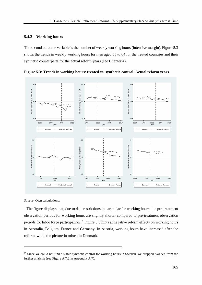
5. Dangerous Flexible Retirement Reforms – A Supplementary Placebo Analysis across Time
165
5.4.2 Working hours
The second outcome variable is the number of weekly working hours (intensive margin). Figure 5.3
shows the trends in weekly working hours for men aged 55 to 64 for the treated countries and their
synthetic counterparts for the actual reform years (see Chapter 4).
Figure 5.3: Trends in working hours: treated vs. synthetic control. Actual reform years
Source: Own calculations.
The figure displays that, due to data restrictions in particular for working hours, the pre-treatment
observation periods for working hours are slightly shorter compared to pre-treatment observation
periods for labor force participation.69 Figure 5.3 hints at negative reform effects on working hours
in Australia, Belgium, France and Germany. In Austria, working hours have increased after the
reform, while the picture in mixed in Denmark.
69 Since we could not find a stable synthetic control for working hours in Sweden, we dropped Sweden from the further analysis (see Figure A.7.2 in Appendix A.7).
30
40
50
Wee
kly W
orki
ng H
ours
age
d 55
-64
1995 2000 2005 2010year
Australia Synthetic Australia
30
40
50
Wee
kly W
orki
ng H
ours
age
d 55
-64
1995 2000 2005 2010year
Austria Synthetic Austria
30
40
50
Wee
kly W
orki
ng H
ours
age
d 55
-64
1990 1995 2000 2005 2010year
Belgium Synthetic Belgium
30
40
50
Wee
kly W
orki
ng H
ours
age
d 55
-64
1990 1995 2000year
Denmark Synthetic Denmark
30
40
50
Wee
kly W
orki
ng H
ours
age
d 55
-64
1985 1990 1995 2000year
France Synthetic France
30
40
50
Wee
kly W
orki
ng H
ours
age
d 55
-64
1985 1990 1995 2000year
Germany Synthetic Germany
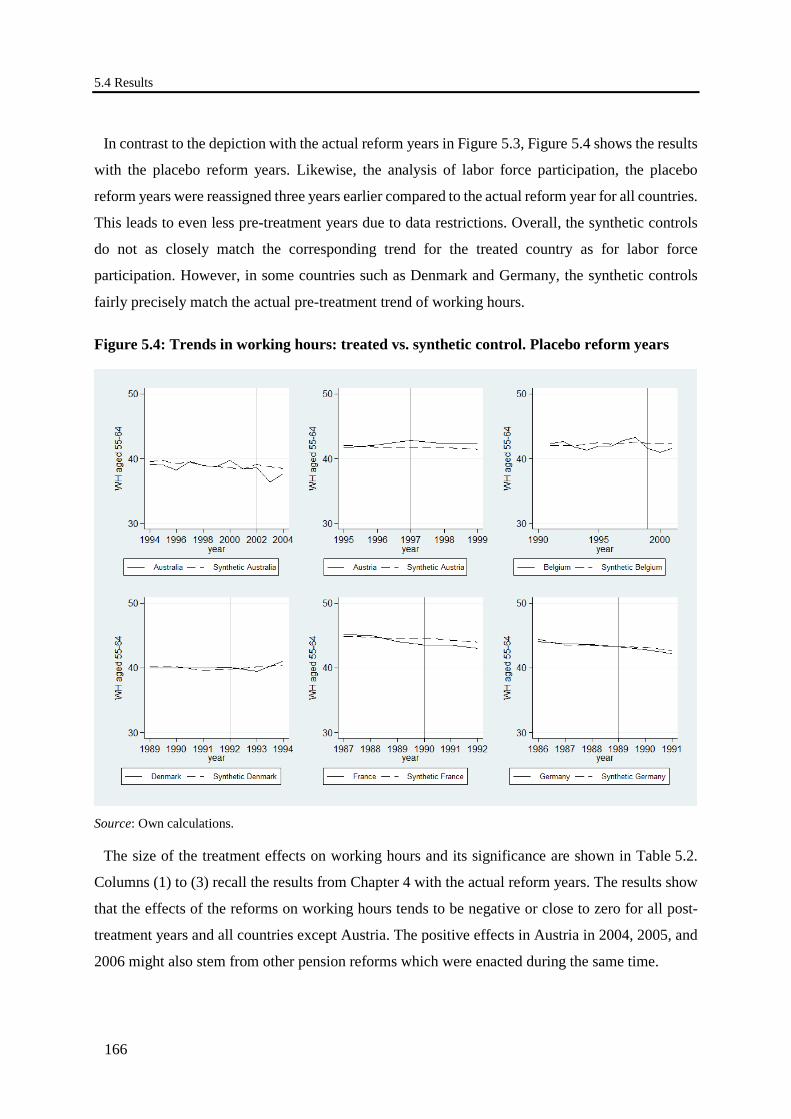
5.4 Results
166
In contrast to the depiction with the actual reform years in Figure 5.3, Figure 5.4 shows the results
with the placebo reform years. Likewise, the analysis of labor force participation, the placebo
reform years were reassigned three years earlier compared to the actual reform year for all countries.
This leads to even less pre-treatment years due to data restrictions. Overall, the synthetic controls
do not as closely match the corresponding trend for the treated country as for labor force
participation. However, in some countries such as Denmark and Germany, the synthetic controls
fairly precisely match the actual pre-treatment trend of working hours.
Figure 5.4: Trends in working hours: treated vs. synthetic control. Placebo reform years
Source: Own calculations.
The size of the treatment effects on working hours and its significance are shown in Table 5.2.
Columns (1) to (3) recall the results from Chapter 4 with the actual reform years. The results show
that the effects of the reforms on working hours tends to be negative or close to zero for all post-
treatment years and all countries except Austria. The positive effects in Austria in 2004, 2005, and
2006 might also stem from other pension reforms which were enacted during the same time.
5. Dangerous Flexible Retirement Reforms – A Supplementary Placebo Analysis across Time
167
Columns (4) to (6) display the yearly treatment effects and pseudo p-values from the in-time
placebo study. As in the analysis of labor force participation, almost all effects disappear when
artificially reassigning the treatment years to placebo reform years three years earlier. The
disappearance of effects on working hours again means that the effects found in Chapter 4 actually
reflect the effects of the flexibility reforms. This interpretation is based, as explained above, on the
initial idea of the in-time placebo studies: The confidence about the validity of results dissipates if
the estimation procedure of the synthetic control method had also produced large effects when
applied to dates where the reforms did not occur. Only in Australia (2003) and France (1990), the
estimation procedure yields occasional significant effects.70 For France, this most likely stems from
a poor synthetic control. Due to data availability, the pre-treatment period is only three years and
therefore does not constitute a solid basis to develop a stable synthetic control. I observe for 1989
that the actual trend of working hours of the treated country and the trend of the synthetic control
drift apart. Regarding Australia, the actual data show a downward spike in 2003 which may explain
the significant effect. However, this effect may be due to a set of reforms of the superannuation
system that happened in 2002 and 2003 (Warren 2008). The placebo reform year therefore most
likely coincides with these other reforms which took place during the same time.
70 Excluding Luxembourg from the synthetic control group in this case does qualitatively not change anything as Luxembourg’s weight in the synthetic control for the outcome variable working hours for Australia is zero and for France only 0.195 (Appendix B, see Table B.2.2 and Table B.5.2).
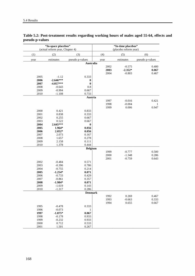
5.4 Results
168
Table 5.2: Post-treatment results regarding working hours of males aged 55-64, effects and pseudo p-values
“In-space placebos” (actual reform year, Chapter 4)
“In-time placebos” (placebo reform year)
(1) (2) (3) (4) (5) (6)
year estimates pseudo p-values year estimates pseudo p-values Australia
2002 -0.575 0.400 2003 -2.352* 0.067 2004 -0.803 0.467
2005 -1.12 0.333 2006 -2.646*** 0 2007 -4.057*** 0 2008 -0.643 0.8 2009 -0.994 0.667 2010 -1.108 0.733
Austria 1997 -0.016 0.421
1998 -0.004 1 1999 0.006 0.947
2000 0.421 0.833 2001 0.838 0.333 2002 0.255 0.667 2003 0.522 0.667 2004 2.645*** 0 2005 1.964* 0.056 2006 2.052* 0.056 2007 2.073 0.167 2008 1.657 0.278 2009 2.158 0.111 2010 1.378 0.444
Belgium 1999 -0.777 0.500
2000 -1.348 0.286 2001 -0.759 0.643
2002 -0.484 0.571 2003 -0.396 0.786 2004 -0.755 0.214 2005 -1.254* 0.071 2006 -0.733 0.429 2007 -0.861 0.357 2008 -1.984* 0.071 2009 -1.619 0.143 2010 -1.317 0.286
Denmark 1992 0.269 0.467
1993 -0.663 0.333 1994 0.655 0.667
1995 -0.478 0.333 1996 -0.073 1 1997 -1.875* 0.067 1998 -0.178 0.933 1999 -0.232 0.933 2000 0.712 0.533 2001 1.501 0.267
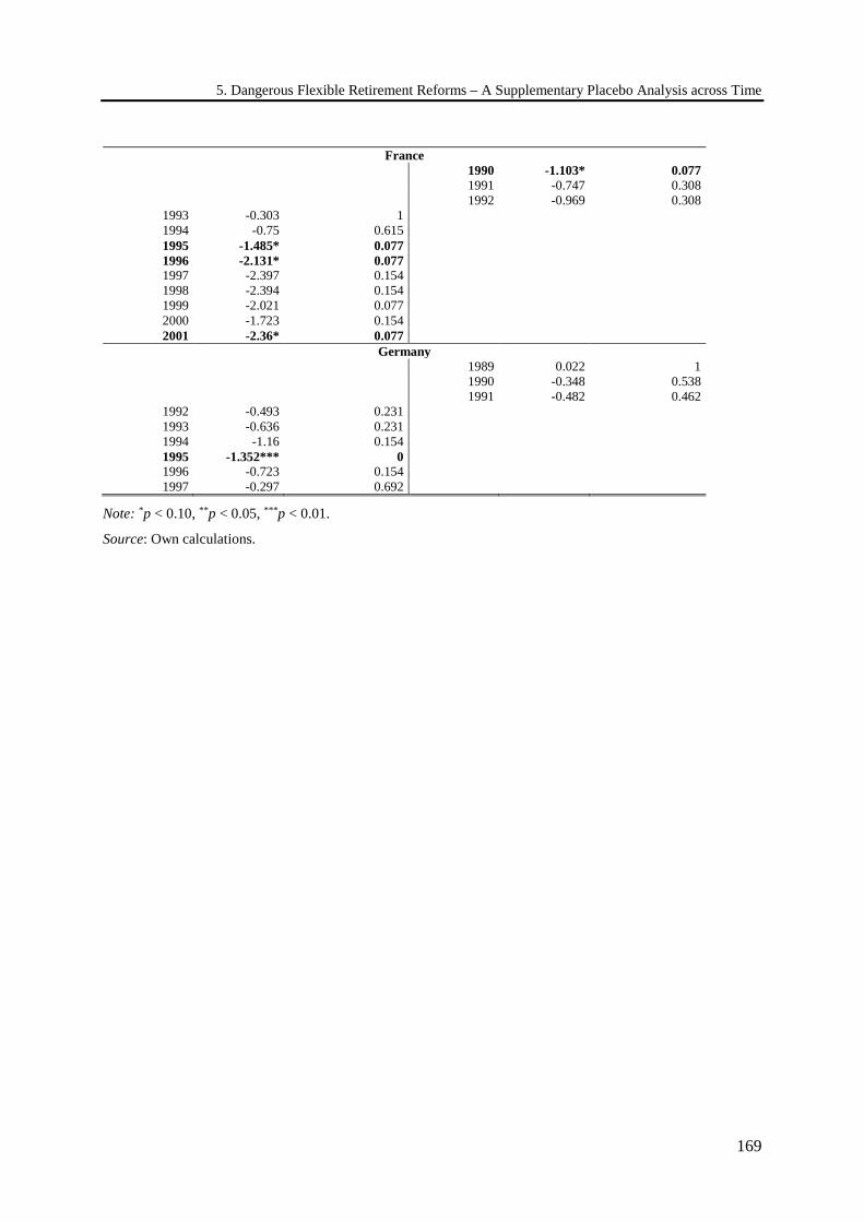
5. Dangerous Flexible Retirement Reforms – A Supplementary Placebo Analysis across Time
169
France 1990 -1.103* 0.077
1991 -0.747 0.308 1992 -0.969 0.308
1993 -0.303 1 1994 -0.75 0.615 1995 -1.485* 0.077 1996 -2.131* 0.077 1997 -2.397 0.154 1998 -2.394 0.154 1999 -2.021 0.077 2000 -1.723 0.154 2001 -2.36* 0.077
Germany 1989 0.022 1
1990 -0.348 0.538 1991 -0.482 0.462
1992 -0.493 0.231 1993 -0.636 0.231 1994 -1.16 0.154 1995 -1.352*** 0 1996 -0.723 0.154 1997 -0.297 0.692
Note: *p < 0.10, **p < 0.05, ***p < 0.01.
Source: Own calculations.
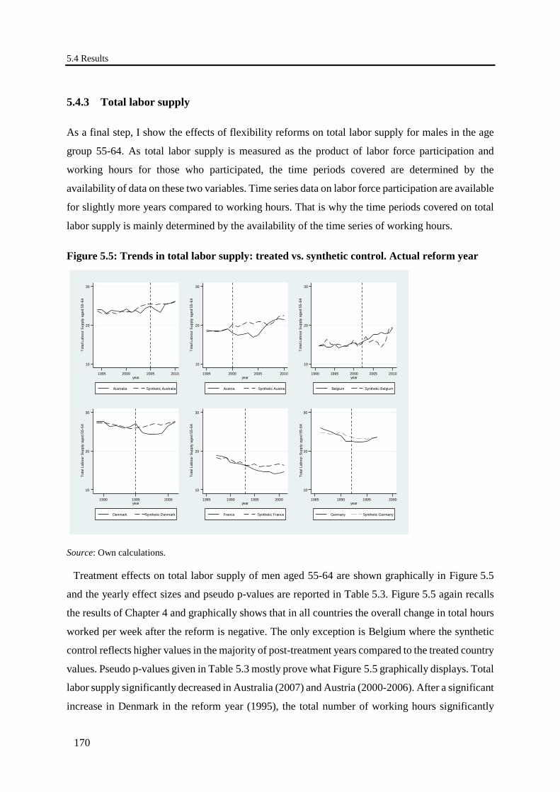
5.4 Results
170
5.4.3 Total labor supply
As a final step, I show the effects of flexibility reforms on total labor supply for males in the age
group 55-64. As total labor supply is measured as the product of labor force participation and
working hours for those who participated, the time periods covered are determined by the
availability of data on these two variables. Time series data on labor force participation are available
for slightly more years compared to working hours. That is why the time periods covered on total
labor supply is mainly determined by the availability of the time series of working hours.
Figure 5.5: Trends in total labor supply: treated vs. synthetic control. Actual reform year
Source: Own calculations.
Treatment effects on total labor supply of men aged 55-64 are shown graphically in Figure 5.5
and the yearly effect sizes and pseudo p-values are reported in Table 5.3. Figure 5.5 again recalls
the results of Chapter 4 and graphically shows that in all countries the overall change in total hours
worked per week after the reform is negative. The only exception is Belgium where the synthetic
control reflects higher values in the majority of post-treatment years compared to the treated country
values. Pseudo p-values given in Table 5.3 mostly prove what Figure 5.5 graphically displays. Total
labor supply significantly decreased in Australia (2007) and Austria (2000-2006). After a significant
increase in Denmark in the reform year (1995), the total number of working hours significantly
10
20
30
Tota
l Lab
our S
uppl
y ag
ed 5
5-64
1995 2000 2005 2010year
Australia Synthetic Australia
10
20
30
Tota
l Lab
our S
uppl
y ag
ed 5
5-64
1995 2000 2005 2010year
Austria Synthetic Austria
10
20
30
Tota
l Lab
our S
uppl
y ag
ed 5
5-64
1990 1995 2000 2005 2010year
Belgium Synthetic Belgium
10
20
30
Tota
l Lab
our S
uppl
y ag
ed 5
5-64
1990 1995 2000year
Denmark Synthetic Denmark
10
20
30
Tota
l Lab
our S
uppl
y ag
ed 5
5-64
1985 1990 1995 2000year
France Synthetic France
10
20
30
Tota
l Lab
our S
uppl
y ag
ed 5
5-64
1985 1990 1995 2000year
Germany Synthetic Germany
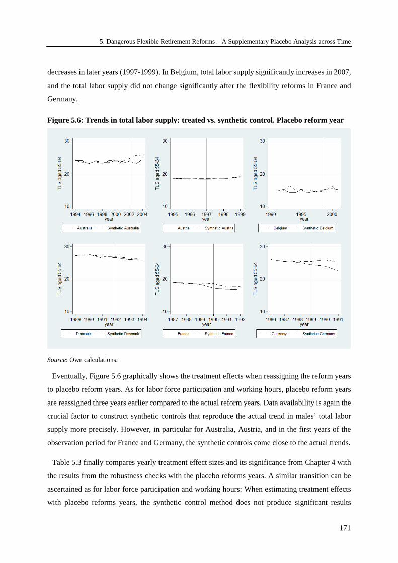
5. Dangerous Flexible Retirement Reforms – A Supplementary Placebo Analysis across Time
171
decreases in later years (1997-1999). In Belgium, total labor supply significantly increases in 2007,
and the total labor supply did not change significantly after the flexibility reforms in France and
Germany.
Figure 5.6: Trends in total labor supply: treated vs. synthetic control. Placebo reform year
Source: Own calculations.
Eventually, Figure 5.6 graphically shows the treatment effects when reassigning the reform years
to placebo reform years. As for labor force participation and working hours, placebo reform years
are reassigned three years earlier compared to the actual reform years. Data availability is again the
crucial factor to construct synthetic controls that reproduce the actual trend in males’ total labor
supply more precisely. However, in particular for Australia, Austria, and in the first years of the
observation period for France and Germany, the synthetic controls come close to the actual trends.
Table 5.3 finally compares yearly treatment effect sizes and its significance from Chapter 4 with
the results from the robustness checks with the placebo reforms years. A similar transition can be
ascertained as for labor force participation and working hours: When estimating treatment effects
with placebo reforms years, the synthetic control method does not produce significant results
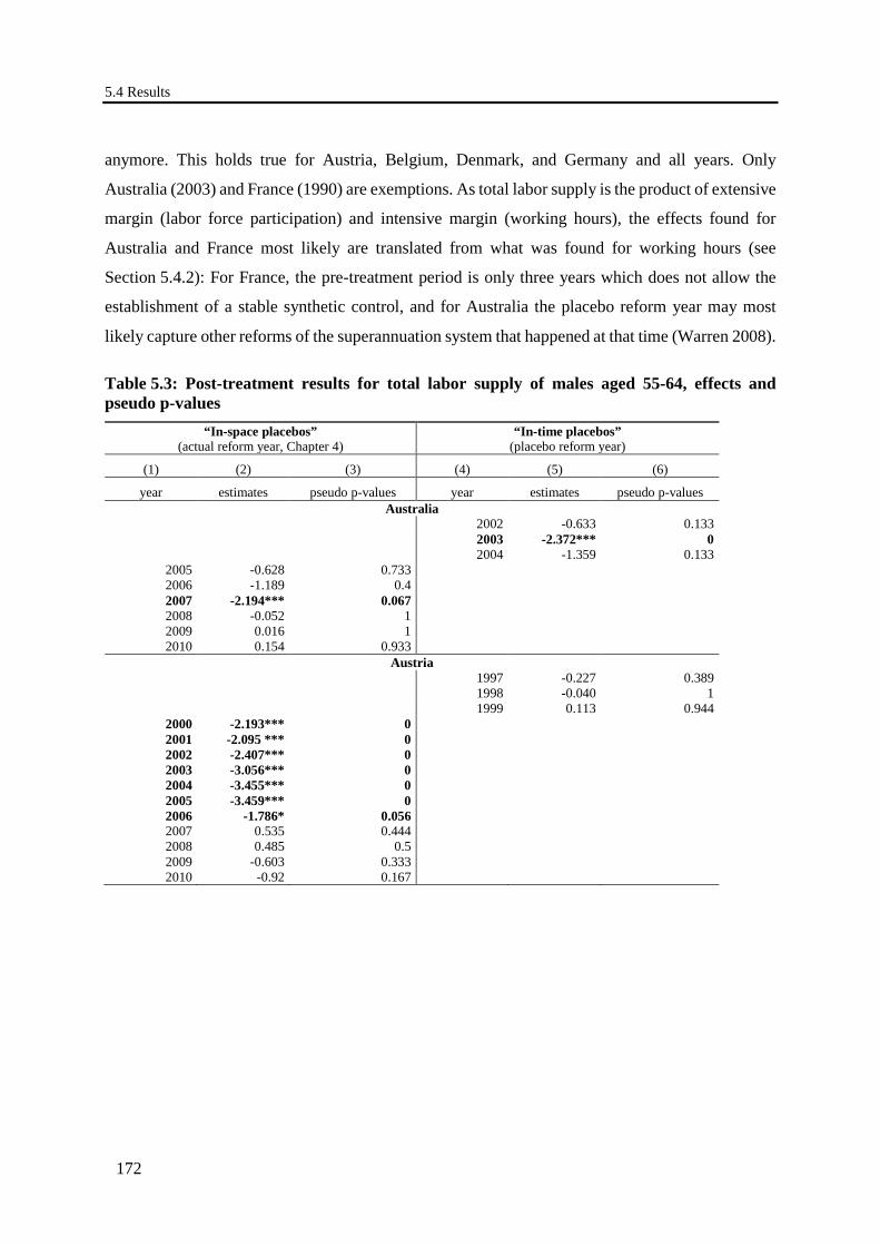
5.4 Results
172
anymore. This holds true for Austria, Belgium, Denmark, and Germany and all years. Only
Australia (2003) and France (1990) are exemptions. As total labor supply is the product of extensive
margin (labor force participation) and intensive margin (working hours), the effects found for
Australia and France most likely are translated from what was found for working hours (see
Section 5.4.2): For France, the pre-treatment period is only three years which does not allow the
establishment of a stable synthetic control, and for Australia the placebo reform year may most
likely capture other reforms of the superannuation system that happened at that time (Warren 2008).
Table 5.3: Post-treatment results for total labor supply of males aged 55-64, effects and pseudo p-values
“In-space placebos” (actual reform year, Chapter 4)
“In-time placebos” (placebo reform year)
(1) (2) (3) (4) (5) (6)
year estimates pseudo p-values year estimates pseudo p-values Australia
2002 -0.633 0.133 2003 -2.372*** 0 2004 -1.359 0.133
2005 -0.628 0.733 2006 -1.189 0.4 2007 -2.194*** 0.067 2008 -0.052 1 2009 0.016 1 2010 0.154 0.933
Austria 1997 -0.227 0.389
1998 -0.040 1 1999 0.113 0.944
2000 -2.193*** 0 2001 -2.095 *** 0 2002 -2.407*** 0 2003 -3.056*** 0 2004 -3.455*** 0 2005 -3.459*** 0 2006 -1.786* 0.056 2007 0.535 0.444 2008 0.485 0.5 2009 -0.603 0.333 2010 -0.92 0.167
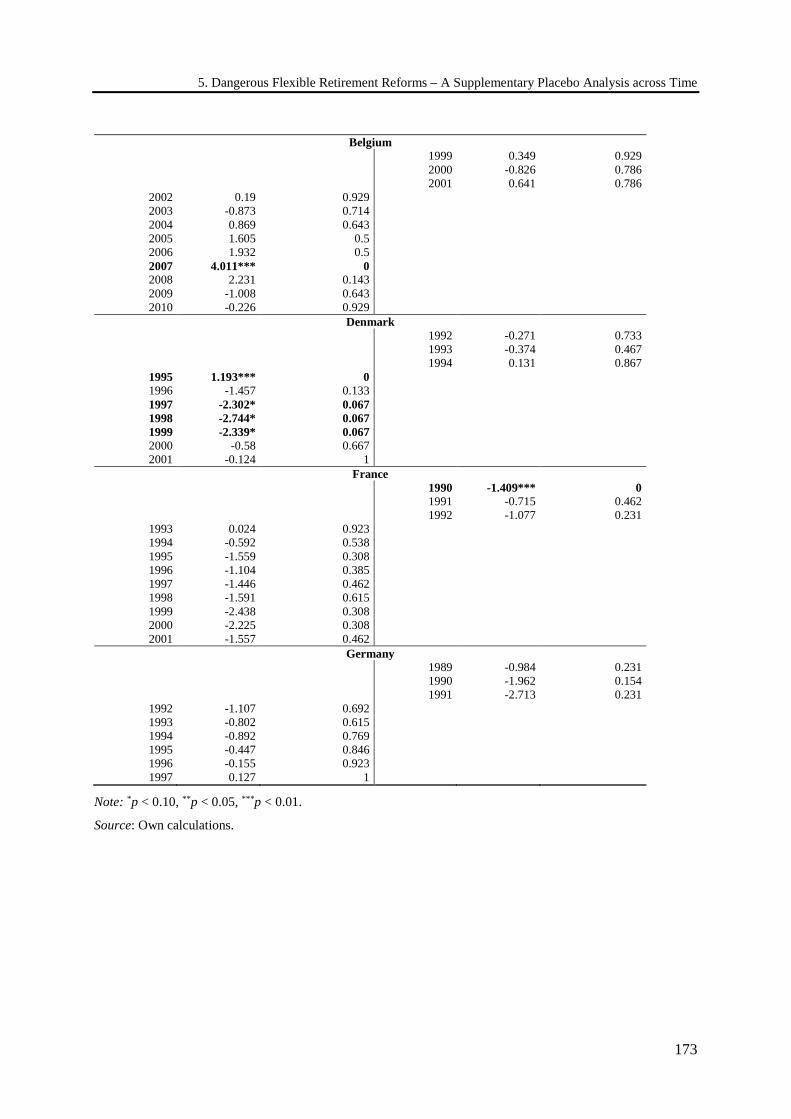
5. Dangerous Flexible Retirement Reforms – A Supplementary Placebo Analysis across Time
173
Belgium 1999 0.349 0.929
2000 -0.826 0.786 2001 0.641 0.786
2002 0.19 0.929 2003 -0.873 0.714 2004 0.869 0.643 2005 1.605 0.5 2006 1.932 0.5 2007 4.011*** 0 2008 2.231 0.143 2009 -1.008 0.643 2010 -0.226 0.929
Denmark 1992 -0.271 0.733
1993 -0.374 0.467 1994 0.131 0.867
1995 1.193*** 0 1996 -1.457 0.133 1997 -2.302* 0.067 1998 -2.744* 0.067 1999 -2.339* 0.067 2000 -0.58 0.667 2001 -0.124 1
France 1990 -1.409*** 0
1991 -0.715 0.462 1992 -1.077 0.231
1993 0.024 0.923 1994 -0.592 0.538 1995 -1.559 0.308 1996 -1.104 0.385 1997 -1.446 0.462 1998 -1.591 0.615 1999 -2.438 0.308 2000 -2.225 0.308 2001 -1.557 0.462
Germany 1989 -0.984 0.231
1990 -1.962 0.154 1991 -2.713 0.231
1992 -1.107 0.692 1993 -0.802 0.615 1994 -0.892 0.769 1995 -0.447 0.846 1996 -0.155 0.923 1997 0.127 1
Note: *p < 0.10, **p < 0.05, ***p < 0.01.
Source: Own calculations.
5.5 Summary and conclusion
174
5.5 Summary and conclusion
Over the past decades, several OECD countries have enacted flexible retirement reforms. According
to politicians, flexibilization is supposed to provide an elegant way to increase older workers’ labor
supply. The model in Chapter 4, however, has shown from a theoretical point of view that flexibility
reforms may have ambiguous effects on labor supply. Therefore, the question whether flexibility
reforms have actually helped to increase older workers’ labor supply remains an empirical one.
In the empirical analysis of Chapter 4, the synthetic control method is used to investigate the effect
of flexibility reforms enacted in different OECD countries between 1992 and 2006. As large sample
inference techniques are problematic in comparative case studies, placebo studies can provide a
remedy to facilitate inference. Following the nomenclature of Abadie et al. (2015), there are two
possibilities of placebo studies: in-space placebos and in-time placebos. To investigate the
significance of the estimates, in-space placebo studies were applied in Chapter 4. This meant an
artificially reassigning of the treatments (i.e. flexibility reform) to members of the synthetic control
group which were not directly exposed to a reform at the same time. The results show that labor
force participation of males aged 55-64 has very little if at all increased in some countries and years
due to the flexibility reforms introduced since the 1990s. At the same time, we find that older men
of the same age group have decreased their weekly working hours. In sum, the reforms have
produced zero to negative effects on total labor supply.
The aim of this chapter is to scrutinize these results by applying in-time placebo studies. The
strategy of in-time placebo studies is to reassign the treatment to dates when then actual reform did
not take place (i.e. a reassignment with respect to time). The idea is to find out whether the synthetic
control method produces significant effects when applied to dates other than the actual reform date.
If this were the case, the confidence about the validity of the results presented in Chapter 4 would
dissipate.
The application of in-time placebo studies, however, reveals that the results of Chapter 4 are stable
to this robustness check. In contrast to the results from the in-space placebo study, reassigning the
reform years to placebo reform years display no perceivable effects. Significant effects diminish in
almost all cases when reassigning the reform dates three years earlier. Remaining effects more likely
stem from poor synthetic controls resulting from data restrictions or from the concurrence of other
reforms.

5. Dangerous Flexible Retirement Reforms – A Supplementary Placebo Analysis across Time
175
Finding a good synthetic control country is crucial for the estimation quality. Yet, a key challenge
of the synthetic control method is that it requires a substantial amount of data. Particularly time
series on working hours for older workers are hard to obtain. The application of placebo reform
years to earlier years reduces the length of pre-treatment periods even more. A higher number of
pre-treatment periods would very likely substantially improve the pre-treatment fit. However, more
data is not available. If one nevertheless does not want to forgo the potential in-time placebo
robustness check, data restrictions remain Achilles’ heel.
176
6. Working Pensioners in Europe
This chapter is single-authored.71
6.1 Introduction
Declining birth rates and increasing life expectancy have caused population aging in many countries
around the world. In many European countries, those dynamics will continue well into the twenty-
first century and will thereby change the age structure within the affected countries substantially
(OECD 2015b). This development puts enormous pressure on old-age provision and has caused a
long-lasting debate on how to make the old-age provision systems more sustainable (Börsch-Supan
and Schnabel 1998, Gruber and Wise 1999, 2004, Börsch-Supan and Coile 2019).
In order to ease the burden of aging societies, a common objective has been to better tap into the
pool of older workers. However, one option of harnessing older workers, namely through increasing
eligibility ages for drawing pension benefits, is not a very popular policy. Therefore, many
governments have enacted flexible retirement options that allow workers to gradually reduce work
71 This chapter uses data from SHARE Wave 6 (DOI:10.6103/SHARE.w6.700), see Börsch-Supan et al. (2013) for methodological details. The SHARE data collection has been funded by the European Commission through FP5 (QLK6-CT-2001-00360), FP6 (SHARE-I3: RII-CT-2006-062193, COMPARE: CIT5-CT-2005-028857, SHARELIFE: CIT4-CT-2006-028812), FP7 (SHARE-PREP: GA N°211909, SHARE-LEAP: GA N°227822, SHARE M4: GA N°261982) and Horizon 2020 (SHARE-DEV3: GA N°676536, SERISS: GA N°654221) and by DG Employment, Social Affairs & Inclusion. Additional funding from the German Ministry of Education and Research, the Max Planck Society for the Advancement of Science, the US National Institute on Aging (U01_AG09740-13S2, P01_AG005842, P01_AG08291, P30_AG12815, R21_AG025169, Y1-AG-4553-01, IAG_BSR06-11, OGHA_04-064, HHSN271201300071C) and from various national funding sources is gratefully acknowledged (see www.share-project.org). In addition, this chapter uses data from the generated Job Episodes Panel (OI: 10.6103/SHARE.jep.700), see Brugiavini et al. (2019b) for methodological details. The Job Episodes Panel release 7.0.0 is based on SHARE Waves 3 and 7 (DOIs: 10.6103/SHARE.w3.700, 10.6103/SHARE.w7.700).
6. Working Pensioners in Europe
177
effort with increasing age. The idea of flexible retirement is to insert a transition period with reduced
work effort between the phases of full-time employment and full retirement and to thereby increase
older workers’ labor supply. The income loss resulting from the work reduction is supposed to be
compensated by drawing (partial) pension benefits or by other compensatory sources (e.g.
governmental subsidies, unemployment insurance funds, occupational pension funds etc. See
Appendix to Chapter 4 for country-specific sources to compensate the income loss).
Assuming that the relative preference for leisure increases when individuals get older, standard
labor market theory predicts that in the absence of constraints workers will gradually reduce work
effort with increasing age. In other words, individuals will remain in the labor market until it
becomes too costly for them to work (see Börsch-Supan et al. 2018 and Chapter 4 of this
dissertation, respectively). Previous literature confirms that workers actually want greater flexibility
and would prefer to reduce their working hours towards their retirement (Gielen 2009, Büsch et
al. 2010, Dorbritz and Micheel 2010, Cihlar et al. 2014).
On the other hand, recent empirical research (OECD 2017) shows that take-up rates of flexible
retirement schemes are still relatively low even though many countries in the European Union have
made it easier for pensioners to combine pension benefits with earnings from employment over the
past decade (OECD 2017, Eurofound 2012). Such simplifications included the introduction of
partial retirement schemes, which allow a combination of part-time work and pension benefits, as
well as relaxing constraints like mandatory retirement regulations, earnings tests, which limit the
additional earnings for recipients of public pension benefits, and minimum hours constraints. While
earnings tests effectively mean a maximum hours constraint, minimum hours constraints are
imposed by the employers. In reality, employers often seem to have an aversion towards part-time
employment (Gustman and Steinmeier 1986, Hutchens and Grace-Martin 2006, Hutchens 2010).
The aim of this study is to investigate this mismatch between what workers wish and standard
labor market theory predicts on the one side, and low take-up rates of flexible retirement schemes
on the other side. For this purpose, I will proceed in two main steps: First, I will focus on individual
factors that are likely part of the explanation why individuals actually decide to become working
pensioners, i.e., to combine pension benefits with work income. Second, I will investigate which of
those factors may be responsible for variation across countries.
6.1 Introduction
178
Overall, there is not much research on this issue. Previous research is fragmented across different
single-country studies (e.g. Graf et al. 2011 for evidence on Austria, Huber et al. 2013 for evidence
on Germany, Ilmakunnas and Ilmakunnas 2006 for evidence on Finland, and Brinch et al. 2015 for
evidence on Norway). The few existing cross-country studies mainly focus on different
motivational aspects in the working pensioners’ decision to continue working as well as on the
sociodemographic composition of the group of working pensioners: OECD (2017) finds that
workers’ and employers’ enthusiasm varies across countries. With respect to the individual, the
attractiveness of combining work and receiving a pension varies across socio-economic groups and
is subject to changing expectations and preferences, financial incentives and individual health.
Eurofound’s (2012) main findings are that the typical working pensioner is still relatively young,
male, highly educated, and living in an urban area or has a mortgage. Although employment rates
of female and medium-educated pensioners are beginning to increase, there is still a considerable
proportion of pensioners who are willing to work but cannot find the right job.
Dingemans et al. (2017) explore potential determinants of working beyond retirement age which
is referred to as “bridge employment”. Individual determinants, such as age, education, pension
income and health, as well as family factors, e.g., marital status and whether the respondents
undertake informal care tasks, appear to have importance why individuals choose bridge
employment. In addition, broader normative and economic societal factors at the country level, such
as the presence of a favorable environment and expenditure on pensions appear to also be relevant.
Dingemans and Henkens (2019) examine differences in life satisfaction between full retirees and
working retirees in Europe. Their results indicate a positive relationship between working after
retirement and life satisfaction for retirees with low pension income without a partner. Furthermore,
working after retirement seems to be most important for life satisfaction in relatively poor countries.
Dingemans and Möhring (2019) examine the role of individual work histories as predictor for
working while receiving a pension. Their results indicate that the larger the share of part-time work
or self-employment over the working career, the higher the likelihood to work while receiving
pension benefits. Those with high occupational status and flexible careers, measured by the number
of job changes experienced, are particularly likely to be in paid work while receiving pension
benefits. In terms of gender, the authors find that divorced women are especially likely to work
while receiving a pension, but only if they did not marry again. The authors conclude that
inequalities that develop over the life course continue to play a role for the decision to be in paid
work while receiving a pension. The last three studies mentioned use data from the Survey of
Health, Ageing and Retirement in Europe (SHARE), as does this study.
6. Working Pensioners in Europe
179
To the best of my knowledge, this study is among the first which explicitly focus on the role that
different pension systems might play by shaping the incentive structures in the decision of whether
to become a working pensioner or not. I add to the existing literature by employing an
internationally comparative view on variables that may play a crucial role why individuals receive
employment income while pension benefit receipt. In addition, I study the variation across countries
by explicitly integrating the pension system into the analysis. The pension system is described by a
set of variables consisting of eligibility ages for (1) normal and (2) early retirement, (3) actuarial
deduction rates for early retirement, (4) a specific “start of the retirement window” if flexible
retirement schemes allow an earlier take-up, whether pension schemes comprise of (5) earnings
tests, and (6) the replacement rate which shows the level of pension benefits relative to earnings
from employment.
The remainder of the chapter is as follows: Section 6.2 provides theoretical background and
connects the theory to institutional details across countries. After a description of the data in
Section 6.3, the empirical analysis in Section 6.4 proceeds in two parts. First, I study the within-
country variation by analyzing variable sets which influence whether individuals have earnings
from employment while pension receipt and therefore qualify as working pensioners (Part I). By
applying counterfactual simulations, I subsequently investigate the cross-country variation (Part II).
Section 6.5 concludes that working pensioners are not a very broad phenomenon in Europe. There
are, however, substantial differences across countries. The study indicates that economic
differences and pension systems likely are driving factors for the cross-country variation.
6.2 Economic theory and institutional details
The theoretical literature has emphasized constraints that may hinder individuals from combining
pension benefits with income from work at the end of their working career. Those constraints
hamper both combining pension benefits and work income without institutional arrangement and
take-up rates of institutionalized flexible retirement schemes (e.g. partial retirement schemes etc.).
I primarily draw on the theoretical background developed in Börsch-Supan et al. 2018 (also see
Chapter 4 of this dissertation). There, constraints have been discussed which may be part of the
explanation of the mismatch between individuals’ preferences for a reduction of work effort with
increasing age and the low take-up rates of flexible retirement schemes. These theoretical thoughts
serve to inspire the choice of institutional variables included in the later empirical analysis in this
study.
6.2 Economic theory and institutional details
180
One constraint are minimum hours constraints. According to the very early work of Gustman and
Steinmeier (1983), employers like to impose a minimum number of working hours since part-time
jobs and flexible hours involve additional fixed costs of work.72 Hutchens and Grace-Martin (2006)
study how and why firms differ in their willingness to permit flexible (“phased”) retirement. They
model a profit-maximizing firm and conclude that, first, a minimum hours constraint can be profit-
maximizing. Second, they state that differences in technology may be the reason why some firms
impose a minimum hours constraint while others do not.
What minimum hours constraints imply for a flexible transition phase from full time employment
to full retirement, is shown in the model of Börsch-Supan et al. (2018): In the absence of constraints,
their model predicts that workers gradually reduce their working hours with increasing age when
their preferences for leisure increase. This corresponds to the standard labor market theory case.
However, employers often do not offer the free choice of working hours. In reality, employers often
impose a minimum hours constraint which might be half-time or even higher. This means that
employees can reduce their working hours only slightly until they reach the employer-imposed
constraint. After that, the minimum hours constraint requires that employees work more hours than
they would have preferred without constraints for some time up to the age at which their loss in
preferred leisure is so large that they retire fully. The existence of minimum hours constraints
therefore restricts the flexibility employees have in their labor supply decisions.
Besides minimum hours constraints imposed by the employers, the pension systems in many
countries comprise of earnings tests. Table 6.1 shows details on earnings tests in the countries under
consideration. Earnings tests limit the amount of income individuals can generate while receiving
pension benefits. Thus, earnings tests effectively mean a constraint on the maximum number of
working hours an individual can work. In many countries, earnings test regulations differ before
and after the statutory eligibility age: Earnings tests often apply before the statutory eligibility age
and usually are lifted after the statutory eligibility age (e.g. Austria, Belgium, Czech Republic,
Estonia, Germany, Italy, Poland, and Slovenia). Table 6.1 also shows that the maximum permissible
earnings are relatively low and, in some cases (e.g. Austria, Belgium, and Germany), substantially
below the equivalent of a half-time job.
72 According to Hurd (1996), team production is another reason why minimum hours constraints exist. Functioning team production requires that most workers are present in the workplace at the same time. See Hurd (1996) and Gustman and Steinmeier (1983) for other possible reasons.
6. Working Pensioners in Europe
181
Hutchens and Grace-Martin (2006) mention that the existence of earnings tests may influence a
firm’s flexible retirement policy. Börsch-Supan et al. (2016) show that the combination of earnings
tests and early retirement incentives can create distinct patterns of labor force exit and pension
claiming age. It can lead to very early pension claiming if maximum hours constraints are abolished
in the environment of non-actuarial adjustment factors for early retirement.
Early retirement is the practice of claiming (early) pension benefits before an individual reaches
the statutory eligibility age and can be claimed after attaining the earliest eligibility age.73
Adjustment factors (i.e. deductions) typically lead to reduced early retirement benefits relative to
the benefits available at the statutory eligibility age. Non-actuarial adjustment factors mean that
actual adjustment factors for early retirement – as they are written in the law – are lower than
actuarially fair. Adjustment factors, which are lower than actuarially fair, make pension benefits
more generous and is the case in most of the countries considered in this study (see Queisser and
Whitehouse 2006, OECD 2015b). Both country-specific earliest eligibility ages and actual
deduction rates, as they are legislated, are also shown in Table 6.1. The generosity of pension
systems, especially in the years before the statutory eligibility age, has a crucial effect on the
retirement decision of individuals: The more generous (early) pension benefits are, the higher the
incentives to retire early (see e.g. Gruber and Wise 2004).
These constraints (i.e. earnings tests, minimum hours constraints, eligibility ages, non-actuarial
adjustment factors) taken together could, at least partially, explain why reported preferences for a
reduction of working hours with increasing age do not match the take-up rates of flexible retirement
schemes. Thus, they will be part in the empirical analysis that follows. Even though the literature
has shown that the role of employers surely plays a role in demanding labor supply of (older)
individuals, the focus of the following empirical analysis is on the supply side and on the role of
pension systems.
73 This chapter follows the nomenclature given in the glossary of Börsch-Supan and Coile (2019).

Table 6.1: Overview of institutional details concerning flexible retirement options and earnings tests
Statutory Eligibility
Age74 (SEA) for public pensions
Earliest Eligibility Age75
(EEA) for public pensions
Flexible retirement option outside the public
pension scheme 76
Start of the flexible
retirement window77
Earnings Tests78 (i.e. limit of additional earnings for recipients of public
pension benefits)
Actuarial deduction
s per year79, in
%
Gross replacement rate80, in %
Mandatory retirement81
Austria 65 (men),
60 (women)
62 (men),
57 (women)
employer-employee agreement on a working time
reduction of between 40% and 60%, subsidized by governmental subsidies
55 (men),
50 (women)
Before SEA: when earnings are above a ceiling of 405.98€ per month, the pension is fully withdrawn; After SEA: no limit
4.2 76.6 Mandatory retirement age for certain groups (e.g. 70 for notaries)
Belgium 65 (men),
65 (women)
60.5 (men),
60.5 (women)
employer-employee agreement on a reduction of
working hours by 20% or 50% for employees aged 50
and older (time credit system), subsidized by governmental subsidies
50 (men),
50 (women)
Before SEA: when annual earnings are above 7,793€ (single) or 11,689€ (dependent child), the pension is reduced by the amount that exceeds the limit. If annual earnings are 25% above the limit, the pension is fully withdrawn for as long as the additional income is higher than the ceiling; After SEA: no limit
0 41.0 Mandatory retirement age is 65 for most civil servants
Czech
Republic
62.8 (men),
61.4 (women)
60 (men),
60 (women) - 60 (men),
60 (women)
Before SEA: only earnings lower than CZK 2,500 per month are allowed; After SEA: no limit
5.6 51.3 None
Denmark 65 (men),
65 (women)
60 (men),
60 (women) - 60 (men),
60 (women)
Before SEA: partial early retirement pension for workers aged between 60 and 65 who continue to work between 12 and 30 hours a week; weekly hours must be reduced by at least seven hours a week or at least one quarter of total hours worked in an average week. After SEA: the full basic pension (795€ per month or 9,540€ per year which is equivalent to around 17% of average earnings) is reduced at a rate of 30% against earned income, if work income exceeds 40,518€ per year (approx. ¾ of average earnings)
0 78.5 Mandatory retirement age is 70 for public servants; for certain groups via collective agreement
74 The statutory eligibility age (SEA) is defined as the age at which workers are eligible for full pension benefits independent of any other qualification. 2013 regulation. 75 The earliest eligibility age is defined as the age at which early retirement is possible, mostly with reduced benefits. 2013 regulation. 76 I consider only non-public-pension institutions that individuals may perceive as occupational institutions and are available before having reached the earliest eligibility age for public pension benefits. The reason for this choice is that the working pensioner definition is based on whether an individual receives either public pension benefits or occupational pension benefits/occupational early retirement benefits. 77 Through the flexible retirement option outside the public pension scheme, the flexible retirement window may start earlier than the earliest eligibility age. If there are flexible retirement schemes outside the public pension system (if column “Flexible retirement option outside the pension system” is available), the start of the flexible retirement window is that of the flexible retirement option outside the public pension system. Otherwise, it is determined by the earliest eligibility age for public pension receipt. 2013 regulation. 78 Earnings tests limit additional earnings for recipients of public pension benefits. 79 Actuarial deductions are a factor used to adjust the pension payments if the worker opts for early retirement. 80 The gross replacement rate stem from the OECD’s database and is defined as gross pension entitlements from mandatory public and private pension schemes divided by gross pre-retirement earnings (see OECD 2014b). 81 The information about the mandatory retirement regulations are widely those of 2016.
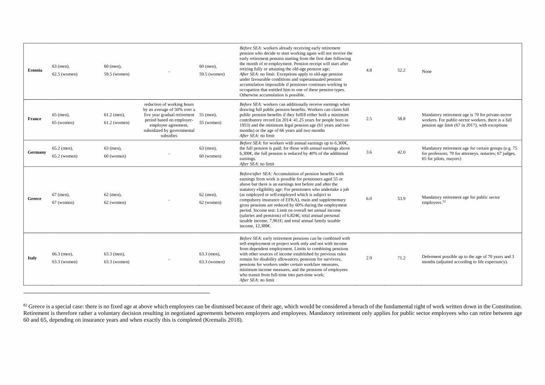
183
Estonia 63 (men),
62.5 (women)
60 (men),
59.5 (women) - 60 (men),
59.5 (women)
Before SEA: workers already receiving early retirement pension who decide to start working again will not receive the early retirement pension starting from the first date following the month of re-employment. Pension receipt will start after retiring fully or attaining the old-age pension age; After SEA: no limit. Exceptions apply to old-age pension under favourable conditions and superannuated pension: accumulation impossible if pensioner continues working in occupation that entitled him to one of these pension types. Otherwise accumulation is possible.
4.8 52.2 None
France 65 (men),
65 (women)
61.2 (men),
61.2 (women)
reduction of working hours by an average of 50% over a five year gradual retirement period based on employer-
employee agreement, subsidized by governmental
subsidies
55 (men),
55 (women)
Before SEA: workers can additionally receive earnings when drawing full public pension benefits. Workers can claim full public pension benefits if they fulfill either both a minimum contributory record (in 2014: 41.25 years for people born in 1953) and the minimum legal pension age (61 years and two months) or the age of 66 years and two months After SEA: no limit
2.5 58.8 Mandatory retirement age is 70 for private-sector workers. For public-sector workers, there is a full pension age limit (67 in 2017), with exceptions
Germany 65.2 (men),
65.2 (women)
63 (men),
60 (women) - 63 (men),
60 (women)
Before SEA: for workers with annual earnings up to 6,300€, the full pension is paid; for those with annual earnings above 6,300€, the full pension is reduced by 40% of the additional earnings. After SEA: no limit
3.6 42.0 Mandatory retirement age for certain groups (e.g. 75 for professors; 70 for attorneys, notaries; 67 judges, 65 for pilots, mayors)
Greece 67 (men),
67 (women)
62 (men),
62 (women) - 62 (men),
62 (women)
Before/after SEA: Accumulation of pension benefits with earnings from work is possible for pensioners aged 55 or above but there is an earnings test before and after the statutory eligibility age: For pensioners who undertake a job (as employed or self-employed which is subject to compulsory insurance of EFKA), main and supplementary gross pensions are reduced by 60% during the employment period. Income test: Limit on overall net annual income (salaries and pensions) of 6,824€; total annual personal taxable income, 7,961€; and total annual family taxable income, 12,389€.
6.0 53.9 Mandatory retirement age for public sector employees.82
Italy 66.3 (men),
63.3 (women)
63.3 (men),
63.3 (women) - 63.3 (men),
63.3 (women)
Before SEA: early retirement pensions can be combined with self-employment or project work only and not with income from dependent employment. Limits to combining pensions with other sources of income established by previous rules remain for disability allowances, pensions for survivors, pensions for workers under certain workfare measures, minimum income measures, and the pensions of employees who transit from full-time into part-time work; After SEA: no limit
2.9 71.2 Deferment possible up to the age of 70 years and 3 months (adjusted according to life expectancy).
82 Greece is a special case: there is no fixed age at above which employees can be dismissed because of their age, which would be considered a breach of the fundamental right of work written down in the Constitution. Retirement is therefore rather a voluntary decision resulting in negotiated agreements between employers and employees. Mandatory retirement only applies for public sector employees who can retire between age 60 and 65, depending on insurance years and when exactly this is completed (Kremalis 2018).
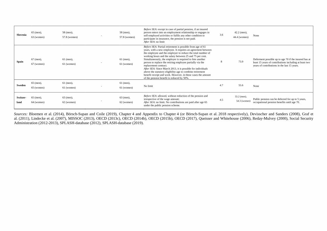
Slovenia 65 (men),
63 (women)
58 (men),
57.8 (women) - 58 (men),
57.8 (women)
Before SEA: except in case of partial pension, if an insured person enters into an employment relationship or engages in self-employed activities or fulfils any other condition to participate in insurance, the pension is not paid. After SEA: no limit
3.6 42.2 (men),
44.4 (women) None
Spain 67 (men),
67 (women)
61 (men),
61 (women) - 61 (men),
61 (women)
Before SEA: Partial retirement is possible from age of 61 years, with a new employee. It requires an agreement between the employee and the employer to reduce the total number of working hours and the salary between 25 and 75 per cent. Simultaneously, the employer is required to hire another person to replace the retiring employee partially via the replacement contract. After SEA: Since March 2013, it is possible for individuals above the statutory eligibility age to combine retirement benefit receipt and work. However, in these cases the amount of the pension benefit is reduced by 50%.
8 73.9 Deferment possible up to age 70 if the insured has at least 15 years of contributions including at least two years of contributions in the last 15 years.
Sweden 65 (men),
65 (women)
61 (men),
61 (women) - 61 (men),
61 (women) No limit 4.7 55.6 None
Switzer-
land
65 (men),
64 (women)
63 (men),
62 (women) - 63 (men),
62 (women)
Before SEA: allowed, without reduction of the pension and irrespective of the wage amount; After SEA: no limit. No contributions are paid after age 65 under the public pension scheme.
4.5 55.2 (men),
54.3 (women) Public pension can be deferred for up to 5 years, occupational pension benefits until age 70.
Sources: Bloemen et al. (2014), Börsch-Supan and Coile (2019), Chapter 4 and Appendix to Chapter 4 (or Börsch-Supan et al. 2018 respectively), Devisscher and Sanders (2008), Graf et al. (2011), Lindecke et al. (2007), MISSOC (2013), OECD (2013c), OECD (2014b), OECD (2015b), OECD (2017), Queisser and Whitehouse (2006), Reday-Mulvey (2000), Social Security Administration (2012-2013), SPLASH-database (2012), SPLASH-database (2019).
6. Working Pensioners in Europe
185
6.3 Data and variables
6.3.1 SHARE data and other data
The individual level data required for the empirical analysis come from SHARE (see Börsch-Supan
et al. 2013). SHARE is a multidisciplinary and cross-national panel database of micro data on
health, socio-economic status and social and family networks of individuals aged 50 or older.
SHARE is a representative survey and was conducted for the first time for eleven European
countries in 2004. Since then, the scope of the survey has expanded in biennial survey waves; it
now covers more than 140,000 individuals in 28 countries. This study uses data from Wave 6
collected in 2015 and integrates 13 countries in the analysis (see Footnote 87 below for the rationale
behind the country selection).
Additionally, I use information to describe the pension system and macro data to control for the
economic situation. Information on gross domestic product (GDP, per capita), labor force
participation rates (LFPR, age 55–64) and the replacement rate (RR, gross) stem from the OECD’s
database (see OECD 2013d, OECD 2013e, and OECD 2014b).83 To describe the pension system,
I use information from various sources given in the list of sources to Table 6.1.
6.3.2 Variables and sample selection
Dependent variable. The dependent variable in the current study is an indicator variable which
equals one if an individual is characterized as working pensioner and zero otherwise. A working
pensioner is identified by focusing on the income sources of older individuals reported in SHARE
Wave 6. Hence, the group of pensioners comprises those who report receiving income from (1) a
public old-age pension, (2) income from a public early retirement or pre-retirement pension, or (3)
report receiving occupational pension benefits/occupational early retirement benefits in the last
year. Accordingly, the group of workers are those individuals who report (1) having received wages,
salaries or other earnings from dependent employment or (2) any income from self-employment or
work for a family business in the last year. Pensioners who at the same time meet the definition of
a worker are classified as working pensioner. Due to data restrictions, I was not able to establish
specific thresholds on earnings or weekly hours of working pensioners, respectively. The same
83 Table C.1 shows numbers for GDP and LFPR (age 55–64) by countries.

6.3 Data and variables
186
holds true for the length working pensioners simultaneously receive both earnings from
employment and pension benefits. In many cases, this period may only be a rather short transition
phase while in other cases it may last longer. The investigation of how long working pensioners
actually stay in the transition period remains open for future research. In addition, I focus on public
pension benefits and occupational pension benefits only. In the single countries other labor market
institutions may play a role in the context of working pensioners as well. The examination of other
labor market institutions should be the objective of future research to obtain a better understanding.
At first glance, the simple definition of working pensioners seems straightforward and has been
applied in previous literature. However, the yearly character of the SHARE employment data might
lead to mismeasurement. Since all questions relevant to the definition of working pensioners refer
to the year preceding the interview, the following problem could arise: If somebody has been in full
employment in the first part of the year, e.g. from January until June, and has started to claim
pension benefits at some point later that year, e.g. in July, she indicates both income from work and
pension income for the last year in the interview. However, the two sorts of income may well have
been received in consecutive periods rather than simultaneously. The latter is required to meet the
definition of a working pensioner. My definition adjusts for this potential mismeasurement problem
by classifying all individuals who retired in 2014 and 2015 and do not report having worked
continuously since the last interview not as working pensioners but as pensioners.84 This approach
leads to conservative estimates for the number of working pensioners which tend to underestimate
the number of working pensioners and simultaneously overstate the number of pensioners.
84 Figure C.1 graphically shows the potential mismeasurement to provide a more intuitive depiction of the problem.
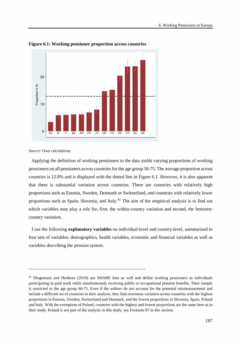
6. Working Pensioners in Europe
187
Figure 6.1: Working pensioner proportion across countries
Source: Own calculations.
Applying the definition of working pensioners to the data yields varying proportions of working
pensioners on all pensioners across countries for the age group 50-75. The average proportion across
countries is 12.8% and is displayed with the dotted line in Figure 6.1. However, it is also apparent
that there is substantial variation across countries. There are countries with relatively high
proportions such as Estonia, Sweden, Denmark or Switzerland, and countries with relatively lower
proportions such as Spain, Slovenia, and Italy.85 The aim of the empirical analysis is to find out
which variables may play a role for, first, the within-country variation and second, the between-
country variation.
I use the following explanatory variables on individual-level and country-level, summarized to
four sets of variables: demographics, health variables, economic and financial variables as well as
variables describing the pension system.
85 Dingemans and Henkens (2019) use SHARE data as well and define working pensioners as individuals participating in paid work while simultaneously receiving public or occupational pension benefits. Their sample is restricted to the age group 60-75. Even if the authors do not account for the potential mismeasurement and include a different set of countries in their analysis, they find enormous variation across countries with the highest proportions in Estonia, Sweden, Switzerland and Denmark, and the lowest proportions in Slovenia, Spain, Poland and Italy. With the exemption of Poland, countries with the highest and lowest proportions are the same here as in their study. Poland is not part of the analysis in this study, see Footnote 87 in this section.
6.3 Data and variables
188
Demographics. I use age (centered), gender, education and marital status to describe the
individual’s demographic characteristics. Education is based on the ISCED-1997-classification.
Low education corresponds to ISCED 0-2, medium education to ISCED 3-4 and high education to
ISCED 5-6. The current marital status is split into the categories married, divorced, widowed or
single. I additionally include a variable to reflect whether the respondent’s partner is in the labor
force or not.
Health. Health plays an important role in the decision to exit the labor market and to start claiming
pension benefits. To describe the individuals’ health status, I use several dimensions: First, I employ
the interviewee’s self-reported health status which is a categorical variable on a five-point scale
from poor (1) to excellent (5). The self-reported health status is one of the most commonly used
measures in public health surveys; it captures various physical, emotional, and social aspects of
health and has been found to predict mortality (e.g. Idler and Benyamini 1997, Jylhä 2009). Self-
reported health may, however, suffer from justification bias (Bound 1991, Sen 2002), meaning
retired pensioners report a worsening of the individual health status to justify retirement. Therefore,
I include additional objective health measures. Grip strength (in kg) is the most objective
measurement of health. The test is performed during the interview. It reflects the overall muscle
status of the respondent and has been linked to mortality in previous research (e.g. Gale et al. 2007).
Functional health is measured by whether the respondent reports having limitations to performing
(instrumental) activities of daily living (ADL and IADL). Finally, I also include the number of
chronic diseases. Individuals report zero to up to twelve chronic diseases.
Economic and financial situation. I include variables on both the individual level (equivalized
household net income and household net worth) and the country level (per-capita GDP and the labor
force participation rate of the age group 55–64) to capture the economic and financial situation. The
information on household net income comes from the SHARE module on household income.
Respondents are asked about the overall income (after taxes and contributions) that the entire
household has in an average month. In order to reflect differences in a household's size and
composition, I divide this number by the weighted sum of household members.86 Household net
worth stems from the imputed dataset and is the sum of net financial assets (i.e. the sum of bank
accounts, bonds, stocks, mutual funds, savings for long-term invests, minus financial liabilities) and
household real assets. The latter is the total value of the household’s main residence (adjusted for
86 The weighting factor is equal one for the first adult and 0.5 for each subsequent person.
6. Working Pensioners in Europe
189
the percentage of house owned), value of the own business (adjusted for the share of own business),
value of cars, value of other real estate minus mortgage on main residence. The variable thus broadly
captures the households’ net worth. Both household net income and household net worth are
adjusted for purchasing power parity to allow cross-country comparisons.
Pension system. I use different variables to describe the pension system. I include the statutory
eligibility age at which an individual becomes eligible for full public pension benefits. Moreover, I
control for an earlier “start of the retirement window” (SRW): On the one hand, this variable
comprises the earliest eligibility age, when public pension benefit receipt is possible (mostly with
reduced benefits). On the other hand, the SWR contains the eligibility age for non-public-pension
institutions if flexible retirement options outside the public pension system are available (see
Table 6.1). However, I consider only non-public-pension institutions that individuals may perceive
as occupational institutions. The reason for this choice is that the working pensioner definition in
this study is based on the receipt of public pension benefits and occupational pension/occupational
early retirement benefits. If there is no broad non-public-pension institution available, the SRW is
the earliest eligibility age for the receipt of public pension benefits. Gender differences in eligibility
ages are taken into account. A dummy variable indicating whether earnings tests apply before the
statutory eligibility age is included as well. Earnings test limit the income individuals are allowed
to earn while receiving pension benefits and these tests apply in most of the countries before the
statutory eligibility age. I additionally integrate the level of actuarial deduction rates, which apply
if individuals claim pension benefits before reaching the statutory eligibility age (usually for each
year of early retirement), and the gross replacement rate which captures the level of pension benefits
relative to earnings from employment. Values for the gross replacement rate stem from the OECD’s
database. The gross replacement rate is defined as gross pension entitlements from mandatory
public and private pension schemes divided by gross pre-retirement earnings (see OECD 2014b). I
finally include two dummy variables indicating whether individuals have reached the earliest
eligibility age and the statutory eligibility age for public pension benefit receipt. Since earliest and
statutory eligibility age are usually cohort- and gender-specific due to their incremental increase in
many countries, the construction of the two dummies uses detailed information on cohort- and
gender-specific eligibility ages from Bucher-Koenen et al. (2019).
Sample selection. The final sample comprises 13 countries, namely Austria, Germany, Sweden,
Spain, Italy, France, Denmark, Greece, Switzerland, Belgium, Czech Republic, Slovenia, and

6.3 Data and variables
190
Estonia.87 The sample is restricted to the age group 50-75. In addition, the sample solely includes
working pensioners and pensioners only receiving public or occupational pension benefits without
simultaneously qualifying as working pensioner. The analytical sample consists of 21,929
observations out of which 2,815 are working pensioners.88
Table 6.2 presents summary statistics of the individual-specific controls for the group of working
pensioners (WP=1) and the group of non-working pensioners (WP=0) as currently delimited.
87 From the sum of countries part of SHARE’s wave 6, I exclude five countries from the analysis for the following reasons: In Portugal the early retirement pathway was closed between 2012 and 2014 due to the financial crisis; Poland also doesn’t offer an early retirement pathway in the general pension system (OECD 2013c). Therefore, important information such as EEA, SRW and actuarial adjustments are not available. For Croatia, there is no comparable gross replacement rate available at the OECD database. Israel’s pension system follows an entirely different logic (National Insurance Institute of Israel 2019). With only N=32, Luxembourg’s number of working pensioners is too small to include in the comparison. 88 Table C.2 shows the number of cases, the gender composition and the average age for the working pensioner group and the group of pensioners by single countries.
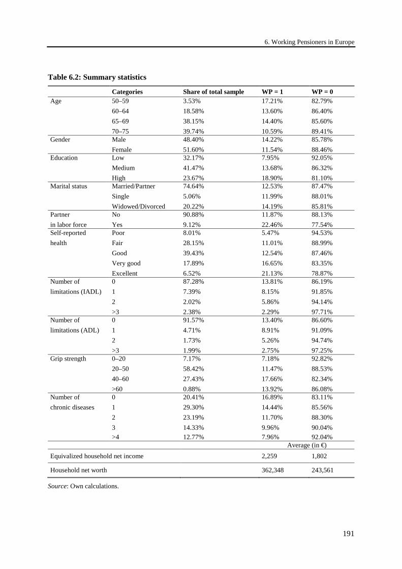
6. Working Pensioners in Europe
191
Table 6.2: Summary statistics Categories Share of total sample WP = 1 WP = 0 Age 50–59 3.53% 17.21% 82.79% 60–64 18.58% 13.60% 86.40% 65–69 38.15% 14.40% 85.60% 70–75 39.74% 10.59% 89.41% Gender Male 48.40% 14.22% 85.78% Female 51.60% 11.54% 88.46% Education Low 32.17% 7.95% 92.05% Medium 41.47% 13.68% 86.32% High 23.67% 18.90% 81.10% Marital status Married/Partner 74.64% 12.53% 87.47% Single 5.06% 11.99% 88.01% Widowed/Divorced 20.22% 14.19% 85.81% Partner No 90.88% 11.87% 88.13% in labor force Yes 9.12% 22.46% 77.54% Self-reported Poor 8.01% 5.47% 94.53% health Fair 28.15% 11.01% 88.99% Good 39.43% 12.54% 87.46% Very good 17.89% 16.65% 83.35% Excellent 6.52% 21.13% 78.87% Number of 0 87.28% 13.81% 86.19% limitations (IADL) 1 7.39% 8.15% 91.85% 2 2.02% 5.86% 94.14% >3 2.38% 2.29% 97.71% Number of 0 91.57% 13.40% 86.60% limitations (ADL) 1 4.71% 8.91% 91.09% 2 1.73% 5.26% 94.74% >3 1.99% 2.75% 97.25% Grip strength 0–20 7.17% 7.18% 92.82% 20–50 58.42% 11.47% 88.53% 40–60 27.43% 17.66% 82.34% >60 0.88% 13.92% 86.08% Number of 0 20.41% 16.89% 83.11% chronic diseases 1 29.30% 14.44% 85.56% 2 23.19% 11.70% 88.30% 3 14.33% 9.96% 90.04% >4 12.77% 7.96% 92.04% Average (in €) Equivalized household net income 2,259 1,802
Household net worth 362,348 243,561
Source: Own calculations.
6.4 Empirical analysis
192
6.4 Empirical analysis
To investigate the variables that may drive the decision to become a working pensioner, I follow
the empirical approach of Börsch-Supan et al. (2020b). The authors analyze the interrelated role of
health and welfare state policies in the decision to take up disability insurance benefits due to work
disability. Since their study aims at investigating the potential causes for reporting a work disability
and/or receiving disability benefits within and between countries, their approach is particularly
suitable to the research interests of this analysis.
The chapter continues as follows: In Section 6.4.1., I study the within-country variation to find
out which variables could play a role in the decision why individuals are working pensioners
(Part I). Section 6.4.2. proceeds with counterfactual analyses to investigate which variables (or
better: variable sets) may be responsible for the between-country variation (Part II).
6.4.1 Part I: within-country variation
6.4.1.1 Regression analysis
What can determine being a working pensioner? To address this question, I estimate a regression
model based on the pooled sample of all countries. Since the dependent variable of interest –
working pensioner – is binary, I estimate the following model by probit estimation:
𝑊𝑊𝐸𝐸𝑖𝑖,𝑐𝑐 = 𝛼𝛼 + 𝑫𝑫𝑫𝑫𝑫𝑫𝑖𝑖,𝑐𝑐′𝜷𝜷 + 𝑯𝑯𝑫𝑫𝑯𝑯𝑯𝑯𝒕𝒕𝑯𝑯𝑖𝑖,𝑐𝑐′𝜸𝜸 + 𝑬𝑬𝑬𝑬𝑬𝑬𝑬𝑬𝑖𝑖,𝑐𝑐′𝜹𝜹 + 𝑷𝑷𝑫𝑫𝑬𝑬𝑖𝑖,𝑐𝑐′𝜽𝜽+ 𝜀𝜀𝑖𝑖,𝑐𝑐 (6.1)
where 𝑖𝑖 indexes individuals and 𝑐𝑐 countries. 𝑊𝑊𝐸𝐸𝑖𝑖,𝑐𝑐 denotes an indicator that takes the value one if
an individual meets the definition of a working pensioner and zero otherwise. The vector 𝑫𝑫𝑫𝑫𝑫𝑫𝑖𝑖,𝑐𝑐
contains the set of individual level demographic characteristics age, gender, education, marital
status as well as the partner’s labor force status as described above. In the vector 𝑯𝑯𝑫𝑫𝑯𝑯𝑯𝑯𝒕𝒕𝑯𝑯𝑖𝑖,𝑐𝑐 the
selected variables from SHARE describing an individual’s health are included (self-perceived
health, ADL, IADL, grip strength as well as the number of chronic diseases). Variables concerning
the economic situation of the respondent or the country that she or he lives in are collected in the
vector 𝑬𝑬𝑬𝑬𝑬𝑬𝑬𝑬𝑖𝑖,𝑐𝑐. The variables describing the individual’s economic situation are her or his
equivalized household net income and the household net worth. Per-capita GDP as well as the labor
force participation rate of the age group 55-64 are included to describe the economic situation of
the respondent’s country. Finally, the vector 𝑷𝑷𝑫𝑫𝑬𝑬𝑖𝑖,𝑐𝑐 comprises all individual or country-specific
variables describing the pension system and the individual’s status within that system. On the
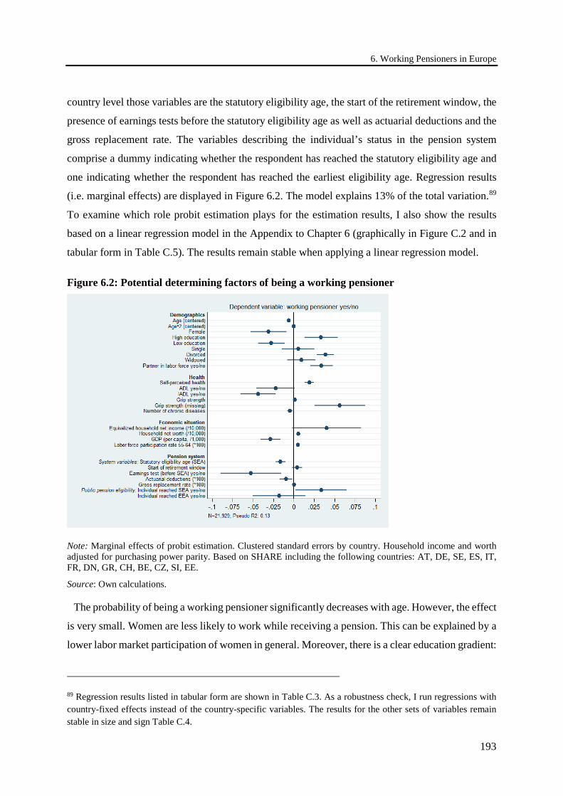
6. Working Pensioners in Europe
193
country level those variables are the statutory eligibility age, the start of the retirement window, the
presence of earnings tests before the statutory eligibility age as well as actuarial deductions and the
gross replacement rate. The variables describing the individual’s status in the pension system
comprise a dummy indicating whether the respondent has reached the statutory eligibility age and
one indicating whether the respondent has reached the earliest eligibility age. Regression results
(i.e. marginal effects) are displayed in Figure 6.2. The model explains 13% of the total variation.89
To examine which role probit estimation plays for the estimation results, I also show the results
based on a linear regression model in the Appendix to Chapter 6 (graphically in Figure C.2 and in
tabular form in Table C.5). The results remain stable when applying a linear regression model.
Figure 6.2: Potential determining factors of being a working pensioner
Note: Marginal effects of probit estimation. Clustered standard errors by country. Household income and worth adjusted for purchasing power parity. Based on SHARE including the following countries: AT, DE, SE, ES, IT, FR, DN, GR, CH, BE, CZ, SI, EE.
Source: Own calculations.
The probability of being a working pensioner significantly decreases with age. However, the effect
is very small. Women are less likely to work while receiving a pension. This can be explained by a
lower labor market participation of women in general. Moreover, there is a clear education gradient:
89 Regression results listed in tabular form are shown in Table C.3. As a robustness check, I run regressions with country-fixed effects instead of the country-specific variables. The results for the other sets of variables remain stable in size and sign Table C.4.
6.4 Empirical analysis
194
The summary statistics in Table 6.2 have shown that in the group of low-educated individuals only
approximately 8% are working pensioners, while among the high-educated individuals almost 19%
work while receiving a pension. This correlation translates to the regression results: High-educated
individuals are more likely to retire flexibly and pensioners with low education are less likely to
simultaneously receive employment income. This may be explained by different occupational types.
Jobs in the low-education sector are more often physically demanding. Individuals suffering from
a physically demanding job might be forced to retire fully. Marital status as well plays a role for the
decision to combine pension income and work income. While being single and widowed compared
to married individuals does not have an effect, divorced individuals are more likely to be a working
pensioner. This could result from financial needs. Divorced individuals might have experienced a
negative income shock due to the divorce which they try to compensate with additional earnings
through receiving a pension. These findings are in line with the results established by Dingemans
and Möhring (2019). They found that divorced women are especially likely to be a working
pensioner if they did not marry again. In contrast, singles are accustomed to their income position
and widowed individuals may be eligible for survivor benefits. If the partner still is in the labor
force, working while receiving a pension gets significantly more likely.
As expected, health is an important variable set. The self-reported health status has a positive
impact on the likelihood of being a working pensioner, i.e., the higher the self-rated heath status,
the higher the probability to become a working pensioner. This finding matches the summary
statistics in Table 6.2. The better the health categories, the higher the proportions of working
pensioners. Reporting at least one limitation with (instrumental) activities of daily living decreases
the probability. However, the vast majority in the sample do not report any limitations with
(instrumental) activities of daily living (see Table 6.2). The probability of working while receiving
a pension decreases also with the number of self-reported chronic diseases. This corresponds to the
descriptive results in Table 6.2, where the proportion of working pensioners in the single categories
of chronic diseases decreases with increasing number of chronic diseases. The most objective health
measure is the individual’s grip strength measured in kilogram. I impute missing values for grip
strength by setting them to zero. I add an additional flag variable to control for these imputed values.
Grip strength only has a very low but still significant effect. The health variables, however, may
suffer from reverse causality: healthier individuals may more likely be working pensioners since
their health allows a continuation of employment. At the same time, however, staying active at the
labor market can influence individual’s health.
6. Working Pensioners in Europe
195
In addition to demographic variables and health variables, I include a set of variables capturing
the economic and financial situation. T-tests reveal that equivalized household net income (p-value
0.000) and household net worth (p-value 0.000) are significantly higher in the group of working
pensioners compared to the group of pensioners. In the regression, both variables have a positive
and significant effect on the probability of being a working pensioner. This could hint at two reverse
effects and may suffer from endogeneity as well: On the one hand, it might indicate that working
pensioners are not mainly motivated by financial motives to keep on working while receiving
pension benefits because they live in comparably wealthier households. On the other hand, this
effect could as well work into the opposite direction: Households with working pensioners are
wealthier because they supplement their pension benefits with income from work. The integration
of the labor force participation rate of the age group 55–64 is supposed to capture the overall
employment possibilities of older workers in the labor market. The labor force participation rate
also has a positive and significant effect, indicating that countries with a more active 55–64 age
group better facilitate flexible transitions into full retirement. Looking at the set of economic
variables, only the amount of per-capita GDP has a negative effect.
The pension system is captured by seven variables described above with effects going in different
directions. However, the seven variables cannot be interpreted in isolation and can be understood
only in conjunction with each other. The start of the flexible retirement window and the existence
of earnings tests before the statutory eligibility age interact with each other. In addition, these
variables interact with the actuarial deductions for early retirement and whether these adjustment
factors are actuarial fair. Taken as a whole, the results suggest that the interactions before the
statutory eligibility age may rather hamper the combination of pension benefits and earnings from
employment. Against this, the comparably higher degree of flexibility past the statutory eligibility
age in many countries may rather ease the combination of employment income and pension benefits
receipt. It may be surprising that the gross replacement rate does not have significant influence. The
reason for this results most likely stems from the fact that the gross replacement rate only varies by
country (in some cases additionally by gender). Thus, this number may suffer from high collinearity
and should not be interpreted in too much detail. It remains open for future research actually which
features of the pension systems are the driving forces in supporting or hampering the combination
of employment income receipt and pension benefit receipt. Likely a combination of features plays
a crucial role.
Overall, the regression analysis indicates that demographic variables as well as health variables,
economic variables and the pension system may be important factors why pensioners
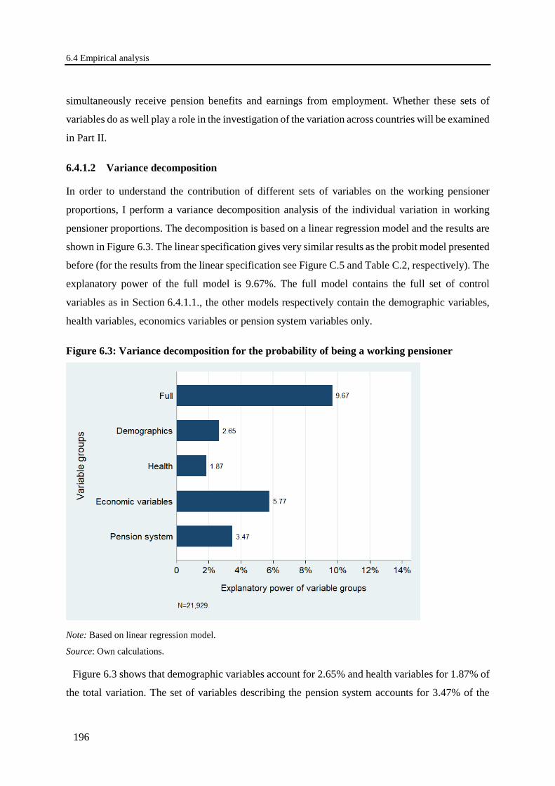
6.4 Empirical analysis
196
simultaneously receive pension benefits and earnings from employment. Whether these sets of
variables do as well play a role in the investigation of the variation across countries will be examined
in Part II.
6.4.1.2 Variance decomposition
In order to understand the contribution of different sets of variables on the working pensioner
proportions, I perform a variance decomposition analysis of the individual variation in working
pensioner proportions. The decomposition is based on a linear regression model and the results are
shown in Figure 6.3. The linear specification gives very similar results as the probit model presented
before (for the results from the linear specification see Figure C.5 and Table C.2, respectively). The
explanatory power of the full model is 9.67%. The full model contains the full set of control
variables as in Section 6.4.1.1., the other models respectively contain the demographic variables,
health variables, economics variables or pension system variables only.
Figure 6.3: Variance decomposition for the probability of being a working pensioner
Note: Based on linear regression model.
Source: Own calculations.
Figure 6.3 shows that demographic variables account for 2.65% and health variables for 1.87% of
the total variation. The set of variables describing the pension system accounts for 3.47% of the

6. Working Pensioners in Europe
197
total variation, while the economic variables contribute to a comparably higher extent to the total
variation (5.77%).
When combining the results from the regression analysis with the variance decomposition
analysis, the choice of variables and the conflation to the four sets of variables seems to be a proper
choice for the following between-country analysis. The aim of the next section is to investigate
whether differences in the variable sets may be responsible for cross-country variation.

6.4 Empirical analysis
198
6.4.2 Part II: between-country variation
Why is there large variation in proportions of working pensioners across countries? In order to
answer that question, I perform counterfactual simulations. The idea of counterfactual simulations
is to set explanatory variables to the average across countries to take account of cross-country
differences. Compared to the European average, Italy, for example, has an older population while
Denmark has a younger population. In the counterfactual simulations, these demographic
differences are taken out by substituting the country-specific demographic variables with the
average across countries and predicting country proportions if Italy and Denmark had the same
demographics.
The procedure is as follows: I estimate the same model as given in Equation 6.1 by probit
estimation to predict the working pensioner proportions for each country. For the baseline
prediction, I use all variables as they are. The counterfactual simulations are executed with specific
sets of variables (i.e. demographics, health, economic variables, pension system) set to the average
across all countries. This way, I predict the working pensioner share as if everybody had the same
characteristics in a specific set of variables as the average of all countries.90
Figure 6.4 presents the main result of this section by comparing the predicted working pensioner
proportions with counterfactual simulation results if the demographic variables, health variables,
economic variables and variables describing the pension system are set to the average across all
countries. The predicted average working pensioner proportion across all countries, represented by
the dotted line, is 12.8%. The countries are sorted by the baseline proportions.
I first take out demographic differences by equalizing age, gender, education, marital status and
the partner information. I then predict the working pensioner share as if all countries had the same
demographic structure. The results are shown in Figure 6.4 by comparing the counterfactual
simulation with the baseline results. Equalizing the demographic structure does not change much,
as indicated by the first and the second bar for each country. Therefore, demographic differences
do not appear to be the main cause of the between-country variation.
90 To verify which role probit estimation plays for the estimation results, I show the counterfactual simulations based on linear regression in Figure C.3 (see the Appendix to Chapter 6). The results remain stable when applying a linear regression model.
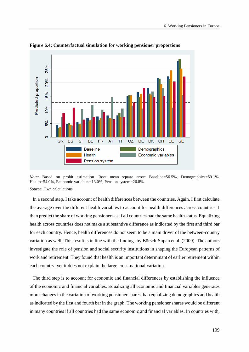
6. Working Pensioners in Europe
199
Figure 6.4: Counterfactual simulation for working pensioner proportions
Note: Based on probit estimation. Root mean square error: Baseline=56.5%, Demographics=59.1%, Health=54.0%, Economic variables=13.0%, Pension system=26.8%.
Source: Own calculations.
In a second step, I take account of health differences between the countries. Again, I first calculate
the average over the different health variables to account for health differences across countries. I
then predict the share of working pensioners as if all countries had the same health status. Equalizing
health across countries does not make a substantive difference as indicated by the first and third bar
for each country. Hence, health differences do not seem to be a main driver of the between-country
variation as well. This result is in line with the findings by Börsch-Supan et al. (2009). The authors
investigate the role of pension and social security institutions in shaping the European patterns of
work and retirement. They found that health is an important determinant of earlier retirement within
each country, yet it does not explain the large cross-national variation.
The third step is to account for economic and financial differences by establishing the influence
of the economic and financial variables. Equalizing all economic and financial variables generates
more changes in the variation of working pensioner shares than equalizing demographics and health
as indicated by the first and fourth bar in the graph. The working pensioner shares would be different
in many countries if all countries had the same economic and financial variables. In countries with,
6.4 Empirical analysis
200
for example, a lower than average labor force participation rate for the age group 55–64 (average
56.6%) such as in France (50.7%), Italy (48.9%), Austria (46.9%), Belgium (45.1%) and Slovenia
(38.4%), working pensioner shares would be much higher if they had the average economic
environment. The opposite holds true for countries with comparably high labor force participation
rates such as in Sweden (78.4%) and Germany (69.1%). In these countries, the shares would be
lower if they had the same economic environment. At the same time, in Sweden (41,060€) and
Germany (33,930€) per-capita GDP is above the average per-capita GDP across all countries
(average 29,980€). This may be another contributing factor to the counterfactually lower shares. In
Slovenia (17,620€) and Greece (17,040€) in contrast, per-capita GDP is below average. This
counterfactually leads to a higher share if Slovenia and Greece had the average economic
environment. Overall, economic differences can be recorded as potential source for between-
country variation.
The last counterfactual simulation is on equalizing the pension system variables across countries
and thus accounts for differences in the pension systems. Once again, working pensioner shares are
predicted as if all countries had the same pension system variables. The rightmost bar shows the
predicted rates if the system characteristics were identical to the average in all countries. The pattern
of working pensioner proportions changes strikingly when equalizing pension systems. The shares
counterfactually decrease, e.g., in Sweden and Switzerland. In both countries, no earnings tests
apply before the statutory eligibility age, thus allowing an unlimited combination of pension
benefits and work income. This makes the pension systems more flexible. The share
counterfactually decreases in Estonia as well when using the average pension variables across
countries. An earnings test applies before the statutory eligibility age in Estonia. However, the
statutory eligibility age is comparably low (63 for men, 62.5 for women, see Table 6.1). Therefore,
individuals are allowed to combine pension income and work income relatively early without any
limitations. Reducing flexibility through equalizing system variables in these countries
counterfactually has a negative effect on working pensioner shares. In Greece and Spain, for
instance, comparably high statutory eligibility ages apply (67 for both men/women). According to
the regression analysis in Part I, the higher the statutory eligibility age, the lower the probability of
being a working pensioner. Conversely, equalizing the statutory eligibility age with the average
across countries (65.3 for males, 64.3 for females) counterfactually yields a higher share. Overall,
in most countries counterfactual simulation leads to working pensioner shares that approach the
overall average proportion. This becomes most apparent when comparing Greece (smallest
proportion at baseline: 4.8%) and Sweden (highest proportion: 27.7%). The proportions in both

6. Working Pensioners in Europe
201
countries are much closer to each other and to the overall average value across all countries when
counterfactually assuming that both countries have the same pension system variables. More
formally, the average deviation from the average across countries (i.e. from the dotted line),
measured as the root mean square error (RMSE), clearly decreases from the baseline value (56.5%)
to the simulation which counterfactually eliminates cross-country differences in variables
describing pension systems (26.8%). This means that differences in the pension systems may also
be responsible for cross-country variation.
Summarizing the results from the counterfactual simulations reveals that economic differences
and differences in pension systems likely are driving factors for the variation in working pensioner
proportions between countries. Demographic differences and health differences do not appear to be
the main causes for cross-country variation. This is supported by the results by Börsch-Supan et al
(2009). They found that institutional differences across countries explain much of the cross-country
differences in work and retirement, while differences in health and demographics only play a minor
role.
6.5 Summary and conclusions
202
6.5 Summary and conclusions
Over the past decade, many countries have made it easier for pensioners to combine pension benefits
with income from work. However, working pensioners are not a broad phenomenon in Europe, even
if survey evidence revealed that substantial shares of individuals prefer a flexible transition into full
retirement.
This study aims at a better understanding of this mismatch. The analysis follows a two-step
procedure: In a first step, I explore variables that influence why individuals combine pension
income and work income at the end of the working career. The regression analysis suggests that
demographic variables, health variables, economic variables as well as the pension system may be
important factors. The second step of the analysis is to find out which variables may account for the
variation in working pensioner proportions across countries. This is realized by performing
counterfactuals simulations. The purpose of counterfactual analysis is to set explanatory variables
to the average across countries to capture cross-country differences. Based on the counterfactual
simulations, I predict working pensioner shares that would prevail in each country, if each
individual had the same characteristics as the average of all countries. Applying counterfactual
simulations indicates that economic differences as well as differences in pension systems may be
responsible for cross-country variation. The theoretical literature has emphasized constraints that
might hinder individuals from combining pension benefits with income from work at the end of
their working career. Some of the constraints are inherent the pension systems. Equalizing theses
constraints across countries suggests that differences in the pension systems could be an important
source for between-country variation. Future research has to show which features of the pension
systems actually are the driving forces.
There has not been much literature with a cross-country focus to date. This article adds to the few
cross-country studies and explicitly integrates variables describing the pension systems. Moreover,
the definition used in this study measures working pensioners more precisely than it has been done
in previous literature.
However, there are still open issues which go beyond the scope of this chapter and remain open
for future research. One question is why working pensioners actually combine pension benefits with
employment income. Next to health limitations and social factors, further motivation might indeed
stem from financial reasons. Overall, it may be the case that individuals in different income classes
have different motives to have income from employment while receiving a pension. A more
comprehensive analysis of the financial motives in the context of varying pension systems,

6. Working Pensioners in Europe
203
therefore, could bring new and more insights. Moreover, the cross-sectional character of the data in
this article does not allow a complete explanation of the transition process from full employment to
either full retirement on a direct way or to a flexible transition phase first. An extension of the
investigation to a panel perspective could help to better understand the actual transition choices. In
addition, this study does not consider how long working pensioners actually stay in the transition
period and how much they earn. This remains open for future research. Moreover, besides public
pension benefits and occupational pension benefits other labor market institutions may play a role
as well. The examination of other labor market institutions in the context of working pensioners
should be the objective of future research to obtain a broader picture.

204
A. Appendix to Chapter 4
A.1 Flexible retirement options and institutional details
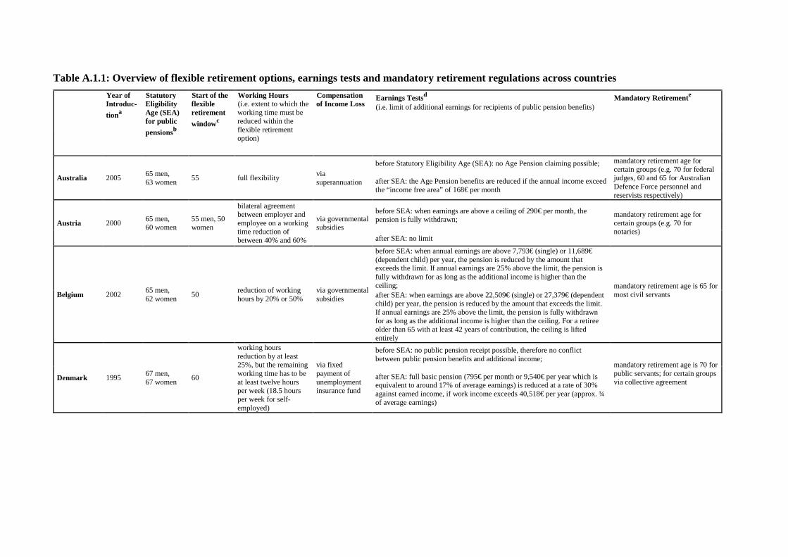
205
Table A.1.1: Overview of flexible retirement options, earnings tests and mandatory retirement regulations across countries Year of
Introduc-tiona
Statutory Eligibility Age (SEA) for public pensionsb
Start of the flexible retirement windowc
Working Hours (i.e. extent to which the working time must be reduced within the flexible retirement option)
Compensation of Income Loss
Earnings Testsd (i.e. limit of additional earnings for recipients of public pension benefits)
Mandatory Retiremente
Australia 2005 65 men, 63 women 55 full flexibility via
superannuation
before Statutory Eligibility Age (SEA): no Age Pension claiming possible; mandatory retirement age for certain groups (e.g. 70 for federal judges, 60 and 65 for Australian Defence Force personnel and reservists respectively)
after SEA: the Age Pension benefits are reduced if the annual income exceed the “income free area” of 168€ per month
Austria 2000 65 men, 60 women
55 men, 50 women
bilateral agreement between employer and employee on a working time reduction of between 40% and 60%
via governmental subsidies
before SEA: when earnings are above a ceiling of 290€ per month, the pension is fully withdrawn;
mandatory retirement age for certain groups (e.g. 70 for notaries)
after SEA: no limit
Belgium 2002 65 men, 62 women 50 reduction of working
hours by 20% or 50% via governmental subsidies
before SEA: when annual earnings are above 7,793€ (single) or 11,689€ (dependent child) per year, the pension is reduced by the amount that exceeds the limit. If annual earnings are 25% above the limit, the pension is fully withdrawn for as long as the additional income is higher than the ceiling; mandatory retirement age is 65 for
most civil servants
after SEA: when earnings are above 22,509€ (single) or 27,379€ (dependent child) per year, the pension is reduced by the amount that exceeds the limit. If annual earnings are 25% above the limit, the pension is fully withdrawn for as long as the additional income is higher than the ceiling. For a retiree older than 65 with at least 42 years of contribution, the ceiling is lifted entirely
Denmark 1995 67 men, 67 women 60
working hours reduction by at least 25%, but the remaining working time has to be at least twelve hours per week (18.5 hours per week for self-employed)
via fixed payment of unemployment insurance fund
before SEA: no public pension receipt possible, therefore no conflict between public pension benefits and additional income;
mandatory retirement age is 70 for public servants; for certain groups via collective agreement
after SEA: full basic pension (795€ per month or 9,540€ per year which is equivalent to around 17% of average earnings) is reduced at a rate of 30% against earned income, if work income exceeds 40,518€ per year (approx. ¾ of average earnings)
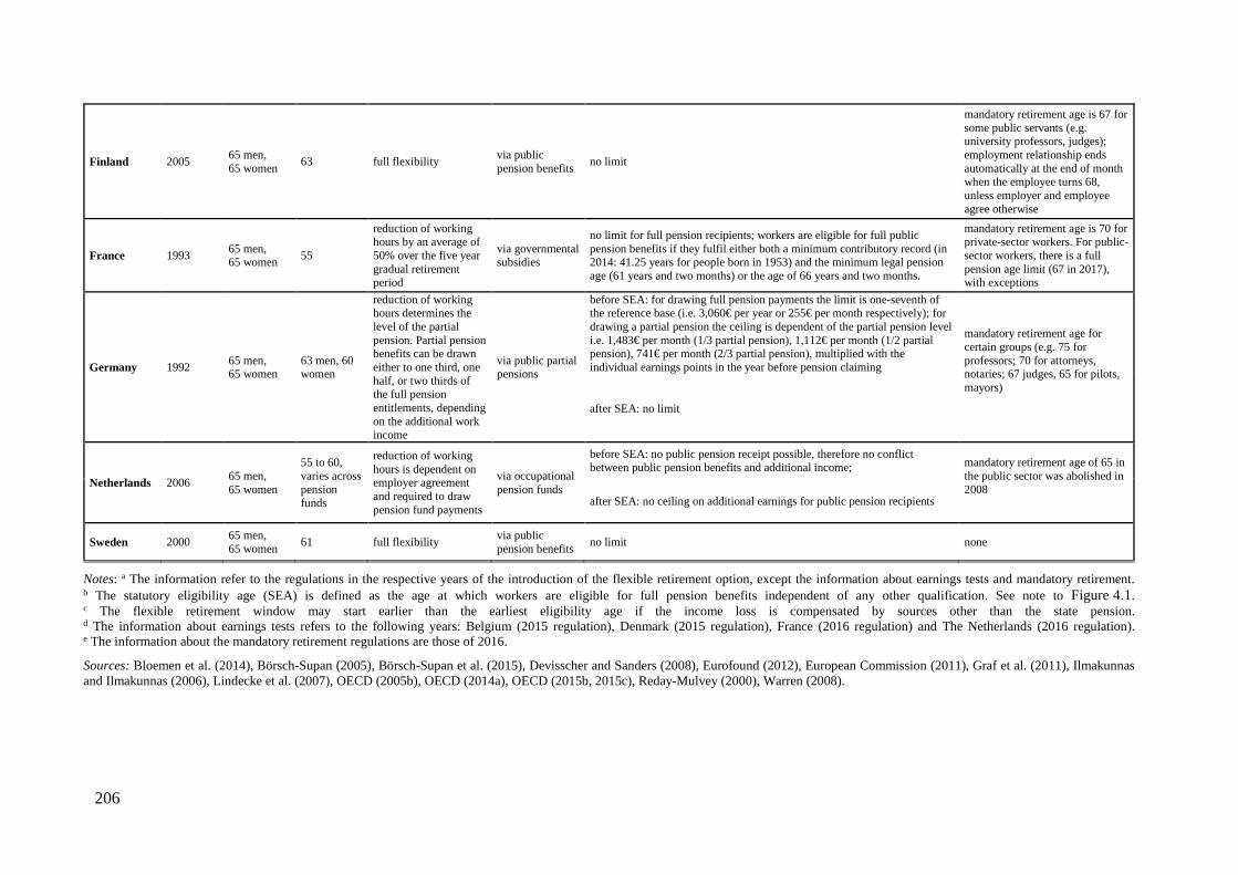
206
Finland 2005 65 men, 65 women 63 full flexibility via public
pension benefits no limit
mandatory retirement age is 67 for some public servants (e.g. university professors, judges); employment relationship ends automatically at the end of month when the employee turns 68, unless employer and employee agree otherwise
France 1993 65 men, 65 women 55
reduction of working hours by an average of 50% over the five year gradual retirement period
via governmental subsidies
no limit for full pension recipients; workers are eligible for full public pension benefits if they fulfil either both a minimum contributory record (in 2014: 41.25 years for people born in 1953) and the minimum legal pension age (61 years and two months) or the age of 66 years and two months.
mandatory retirement age is 70 for private-sector workers. For public-sector workers, there is a full pension age limit (67 in 2017), with exceptions
Germany 1992 65 men, 65 women
63 men, 60 women
reduction of working hours determines the level of the partial pension. Partial pension benefits can be drawn either to one third, one half, or two thirds of the full pension entitlements, depending on the additional work income
via public partial pensions
before SEA: for drawing full pension payments the limit is one-seventh of the reference base (i.e. 3,060€ per year or 255€ per month respectively); for drawing a partial pension the ceiling is dependent of the partial pension level i.e. 1,483€ per month (1/3 partial pension), 1,112€ per month (1/2 partial pension), 741€ per month (2/3 partial pension), multiplied with the individual earnings points in the year before pension claiming
mandatory retirement age for certain groups (e.g. 75 for professors; 70 for attorneys, notaries; 67 judges, 65 for pilots, mayors) after SEA: no limit
Netherlands 2006 65 men, 65 women
55 to 60, varies across pension funds
reduction of working hours is dependent on employer agreement and required to draw pension fund payments
via occupational pension funds
before SEA: no public pension receipt possible, therefore no conflict between public pension benefits and additional income; mandatory retirement age of 65 in
the public sector was abolished in 2008 after SEA: no ceiling on additional earnings for public pension recipients
Sweden 2000 65 men, 65 women 61 full flexibility via public
pension benefits no limit none
Notes: a The information refer to the regulations in the respective years of the introduction of the flexible retirement option, except the information about earnings tests and mandatory retirement. b The statutory eligibility age (SEA) is defined as the age at which workers are eligible for full pension benefits independent of any other qualification. See note to Figure 4.1. c The flexible retirement window may start earlier than the earliest eligibility age if the income loss is compensated by sources other than the state pension. d The information about earnings tests refers to the following years: Belgium (2015 regulation), Denmark (2015 regulation), France (2016 regulation) and The Netherlands (2016 regulation). e The information about the mandatory retirement regulations are those of 2016.
Sources: Bloemen et al. (2014), Börsch-Supan (2005), Börsch-Supan et al. (2015), Devisscher and Sanders (2008), Eurofound (2012), European Commission (2011), Graf et al. (2011), Ilmakunnas and Ilmakunnas (2006), Lindecke et al. (2007), OECD (2005b), OECD (2014a), OECD (2015b, 2015c), Reday-Mulvey (2000), Warren (2008).

Appendix to Chapter 4
207
A.2 Mathematical appendix to model of stylized flexibility reform
A.2.1 Model without constraints on hours worked (situation after flexibility reform)
s.t. ,
where
Optimal consumption is:
Let’s assume that and
Then optimal hours worked in the first two periods are obtained as follows:
If N is the total number of people in the population, share of retirees=
Total labor supply= .
1 2 3 1 2 3MaxU(c ,c ,c ,l ,l ,l )
1 2 1 2 3wl wl c c c+ = + + 3 0l =
( ) ( )3 3
1 2 3 1 2 31 1
U(c ,c ,c ,l ,l ,l ) 1t tt t
u c v lα= =
= + −∑ ∑
1 2 3 *c c c c= = =
1 2*3
wl wlc
+=
( ) lnt tu c c= ( ) ( )1 ln 1t tv l l− = −
* *1 2
32 3
l lα
= =+
3N
3 3 2. .3 2 3 3 2 3 2 3N N N
α α α+ =
+ + +

Appendix to Chapter 4
208
A.2.2 Model with minimum hours constraints imposed (situation before flexibility reform)
In the second period the individual chooses whether he works or retires. If someone wishes to work in the second
period, he must work for a minimum of hours in that period. In this case and the utility from working
will be denoted by . If someone wishes to retire, the number of hours worked is equal to zero and
the utility from being retired will be denoted by .
If > , individual chooses to retire, he works otherwise.
The maximization of the utility function subject to the budget constraint and hours constraint yields
and
If , the solution of the maximization problem yields
Comparison of with reveals that the individual retires if
= .
There are three cases depending on and :
(a) If = , we have the same problem as if there were no constraints on hours worked. So:
If N is the total number of people in the population, share of retirees=
Total labor supply= .
l **2l l≥
( )** ** **1 2, ,U c l l
( )*** ***1, ,0U c l
( )*** *** ***1 2, ,U c l l ( )** ** **
1 2, ,U c l l
2l l≥
**2l l= **
13
3ll α
α−
=+
2 0l = ***1
33
lα
=+
( )*** *** ***1 2, ,U c l l ( )** ** **
1 2, ,U c l l
α′′ ( )( ) ( )
3ln 1
ln 1 ln 1
l
l lα
− +<
+ + −
α l
32 3
lα
<+
α′
* *1 2
32 3
l lα
= =+
3N
3 3 2. .3 2 3 3 2 3 2 3N N N
α α α+ =
+ + +

Appendix to Chapter 4
209
(b) If = , and if = ,
individual retires in the second period, , ,
Share of retirees=
Total labor supply=
implying that total labor supply is smaller compared to the unconstrained case.
(c) If = , and if = ,
individual works in the second period, , ,
Share of retirees=
Total labor supply= .
Together with , this implies that total labor supply is larger compared to the unconstrained case.
32 3
lα
≥+
α′ α′′ ( )( ) ( )
3ln 1
ln 1 ln 1
l
l lα
− +<
+ + −
***1
33
lα
=+
***2 0l =
23N
3 2.3 3 3 2 3N N N
α α α= <
+ + +
32 3
lα
≥+
α′ α′′ ( )( ) ( )
3ln 1
ln 1 ln 1
l
l lα
− +≥
+ + −
**1
33
ll αα
−=
+**2l l=
3N
( ) ( )3 1 1 2.3 3 3 2 3
l N lN Nα α α
+ += >
+ + +
32 3
lα
≥+
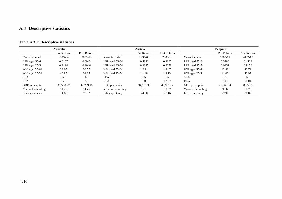
210
A.3 Descriptive statistics
Table A.3.1: Descriptive statistics
Australia Austria Belgium Pre Reform Post Reform Pre Reform Post Reform Pre Reform Post Reform Years included 1983-04 2005-13 Years included 1995-00 2000-13 Years included 1983-01 2002-13 LFP aged 55-64 0.6167 0.6943 LFP aged 55-64 0.4382 0.4667 LFP aged 55-64 0.3780 0.4422 LFP aged 25-54 0.9194 0.9046 LFP aged 25-54 0.9385 0.9258 LFP aged 25-54 0.9251 0.9158 WH aged 55-64 38.05 36.57 WH aged 55-64 42.21 42.47 WH aged 55-64 42.83 40.79 WH aged 25-54 40.85 39.35 WH aged 25-54 41.48 43.13 WH aged 25-54 41.06 40.97 SEA 65 65 SEA 65 65 SEA 65 65 EEA 55 55 EEA 60 62.57 EEA 60 60.04 GDP per capita 31,558.27 42,299.18 GDP per capita 34,967.33 40,991.12 GDP per capita 29,866.34 38,558.17 Years of schooling 11.29 11.46 Years of schooling 9.81 10.32 Years of schooling 9.86 10.78 Life expectancy 74.86 79.32 Life expectancy 74.30 77.16 Life expectancy 72.91 76.82
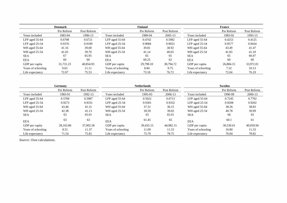
211
Denmark Finland France Pre Reform Post Reform Pre Reform Post Reform Pre Reform Post Reform Years included 1983-94 1996-13 Years included 1989-04 2005-13 Years included 1983-92 1993-13 LFP aged 55-64 0.6708 0.6721 LFP aged 55-64 0.4742 0.5982 LFP aged 55-64 0.4253 0.4125 LFP aged 25-54 0.9376 0.9189 LFP aged 25-54 0.9084 0.9053 LFP aged 25-54 0.9577 0.9434 WH aged 55-64 41.16 39.00 WH aged 55-64 39.81 38.92 WH aged 55-64 43.49 41.47 WH aged 25-54 41.65 39.70 WH aged 25-54 41.14 40.65 WH aged 25-54 41.83 41.10 SEA 67 65.95 SEA 65 65 SEA 65 60.47 EEA 60 60 EEA 60.25 62 EEA 60 60 GDP per capita 31,731.23 40,854.93 GDP per capita 29,798.10 38,794.72 GDP per capita 26,884.15 33,972.01 Years of schooling 9.63 11.11 Years of schooling 8.84 9.75 Years of schooling 7.52 10.13 Life expectancy 72.07 75.53 Life expectancy 73.18 76.72 Life expectancy 72.04 76.19
Germany Netherlands Sweden Pre Reform Post Reform Pre Reform Post Reform Pre Reform Post Reform Years included 1983-91 1992-13 Years included 1995-05 2006-13 Years included 1990-99 2000-13 LFP aged 55-64 0.5769 0.5987 LFP aged 55-64 0.5022 0.6713 LFP aged 55-64 0.7245 0.7702 LFP aged 25-54 0.9273 0.9331 LFP aged 25-54 0.9301 0.9332 LFP aged 25-54 0.9208 0.9202 WH aged 55-64 43.46 41.31 WH aged 55-64 37.31 36.15 WH aged 55-64 38.26 38.83 WH aged 25-54 42.38 41.13 WH aged 25-54 39.59 39.02 WH aged 25-54 40.78 39.99 SEA 65 65.01 SEA 65 65.01 SEA 66 65
EEA 63 63 EEA 61.45 65
EEA 60.1 61
GDP per capita 28,163.86 37,002.58 GDP per capita 39,435.15 44,982.15 GDP per capita 30,530.61 40,059.94 Years of schooling 8.51 11.37 Years of schooling 11.09 11.53 Years of schooling 10.80 11.33 Life expectancy 71.54 75.81 Life expectancy 75.70 78.75 Life expectancy 76.04 78.82
Source: Own calculations.
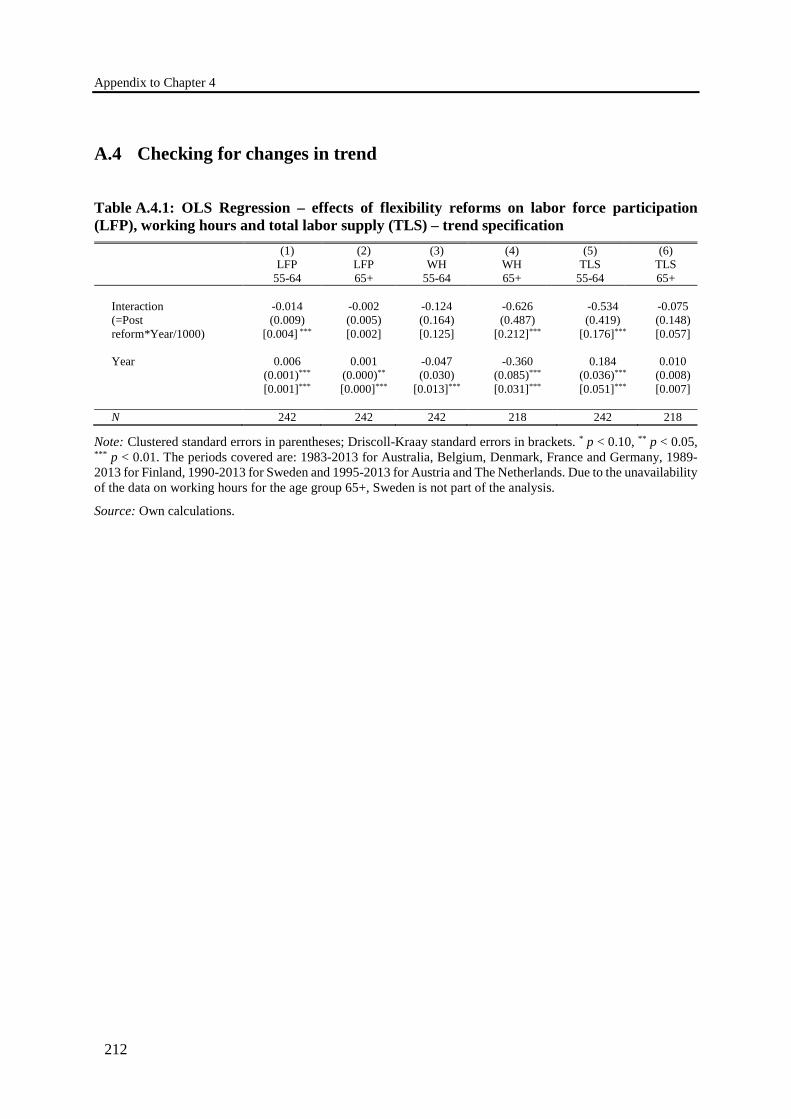
Appendix to Chapter 4
212
A.4 Checking for changes in trend
Table A.4.1: OLS Regression – effects of flexibility reforms on labor force participation (LFP), working hours and total labor supply (TLS) – trend specification
(1) (2) (3) (4) (5) (6) LFP
55-64 LFP 65+
WH 55-64
WH 65+
TLS 55-64
TLS 65+
Interaction -0.014 -0.002 -0.124 -0.626 -0.534 -0.075 (=Post (0.009) (0.005) (0.164) (0.487) (0.419) (0.148) reform*Year/1000) [0.004] *** [0.002] [0.125] [0.212]*** [0.176]*** [0.057] Year 0.006 0.001 -0.047 -0.360 0.184 0.010 (0.001)*** (0.000)** (0.030) (0.085)*** (0.036)*** (0.008) [0.001]*** [0.000]*** [0.013]*** [0.031]*** [0.051]*** [0.007] N 242 242 242 218 242 218
Note: Clustered standard errors in parentheses; Driscoll-Kraay standard errors in brackets. * p < 0.10, ** p < 0.05, *** p < 0.01. The periods covered are: 1983-2013 for Australia, Belgium, Denmark, France and Germany, 1989-2013 for Finland, 1990-2013 for Sweden and 1995-2013 for Austria and The Netherlands. Due to the unavailability of the data on working hours for the age group 65+, Sweden is not part of the analysis.
Source: Own calculations.
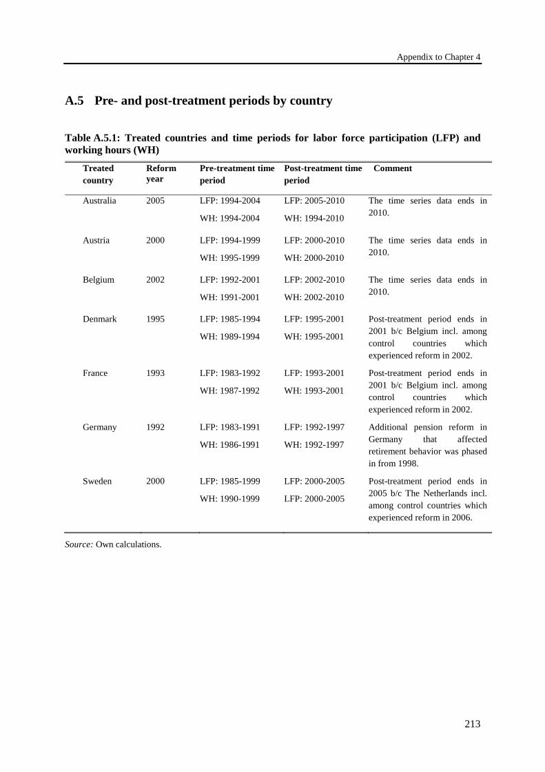
Appendix to Chapter 4
213
A.5 Pre- and post-treatment periods by country
Table A.5.1: Treated countries and time periods for labor force participation (LFP) and working hours (WH)
Treated country
Reform year
Pre-treatment time period
Post-treatment time period
Comment
Australia 2005 LFP: 1994-2004
WH: 1994-2004
LFP: 2005-2010
WH: 1994-2010
The time series data ends in 2010.
Austria 2000 LFP: 1994-1999
WH: 1995-1999
LFP: 2000-2010
WH: 2000-2010
The time series data ends in 2010.
Belgium 2002 LFP: 1992-2001
WH: 1991-2001
LFP: 2002-2010
WH: 2002-2010
The time series data ends in 2010.
Denmark 1995 LFP: 1985-1994
WH: 1989-1994
LFP: 1995-2001
WH: 1995-2001
Post-treatment period ends in 2001 b/c Belgium incl. among control countries which experienced reform in 2002.
France 1993 LFP: 1983-1992
WH: 1987-1992
LFP: 1993-2001
WH: 1993-2001
Post-treatment period ends in 2001 b/c Belgium incl. among control countries which experienced reform in 2002.
Germany 1992 LFP: 1983-1991
WH: 1986-1991
LFP: 1992-1997
WH: 1992-1997
Additional pension reform in Germany that affected retirement behavior was phased in from 1998.
Sweden 2000 LFP: 1985-1999
WH: 1990-1999
LFP: 2000-2005
LFP: 2000-2005
Post-treatment period ends in 2005 b/c The Netherlands incl. among control countries which experienced reform in 2006.
Source: Own calculations.
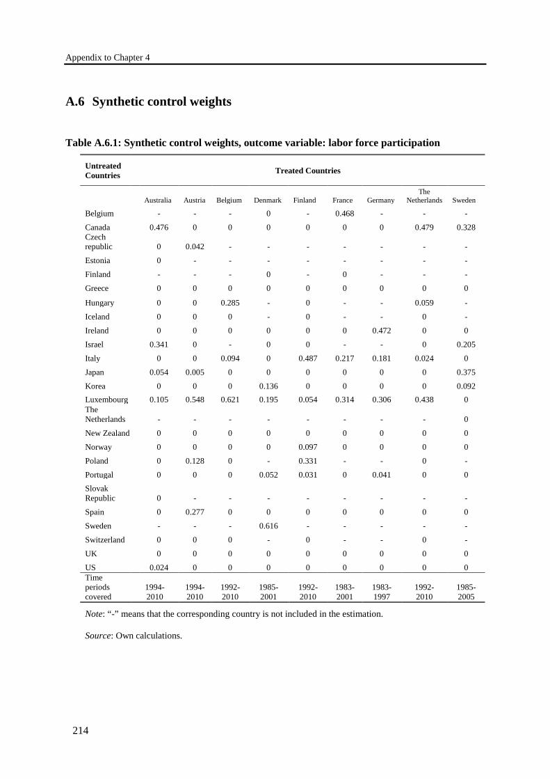
Appendix to Chapter 4
214
A.6 Synthetic control weights
Table A.6.1: Synthetic control weights, outcome variable: labor force participation
Untreated Countries Treated Countries
Australia Austria Belgium Denmark Finland France Germany The
Netherlands Sweden
Belgium - - - 0 - 0.468 - - -
Canada 0.476 0 0 0 0 0 0 0.479 0.328 Czech republic 0 0.042 - - - - - - -
Estonia 0 - - - - - - - -
Finland - - - 0 - 0 - - -
Greece 0 0 0 0 0 0 0 0 0
Hungary 0 0 0.285 - 0 - - 0.059 -
Iceland 0 0 0 - 0 - - 0 -
Ireland 0 0 0 0 0 0 0.472 0 0
Israel 0.341 0 - 0 0 - - 0 0.205
Italy 0 0 0.094 0 0.487 0.217 0.181 0.024 0
Japan 0.054 0.005 0 0 0 0 0 0 0.375
Korea 0 0 0 0.136 0 0 0 0 0.092 Luxembourg 0.105 0.548 0.621 0.195 0.054 0.314 0.306 0.438 0 The Netherlands - - - - - - - - 0
New Zealand 0 0 0 0 0 0 0 0 0
Norway 0 0 0 0 0.097 0 0 0 0
Poland 0 0.128 0 - 0.331 - - 0 -
Portugal 0 0 0 0.052 0.031 0 0.041 0 0 Slovak Republic 0 - - - - - - - -
Spain 0 0.277 0 0 0 0 0 0 0
Sweden - - - 0.616 - - - - -
Switzerland 0 0 0 - 0 - - 0 -
UK 0 0 0 0 0 0 0 0 0
US 0.024 0 0 0 0 0 0 0 0 Time periods covered
1994- 2010
1994-2010
1992-2010
1985- 2001
1992-2010
1983-2001
1983- 1997
1992- 2010
1985- 2005
Note: “-” means that the corresponding country is not included in the estimation.
Source: Own calculations.
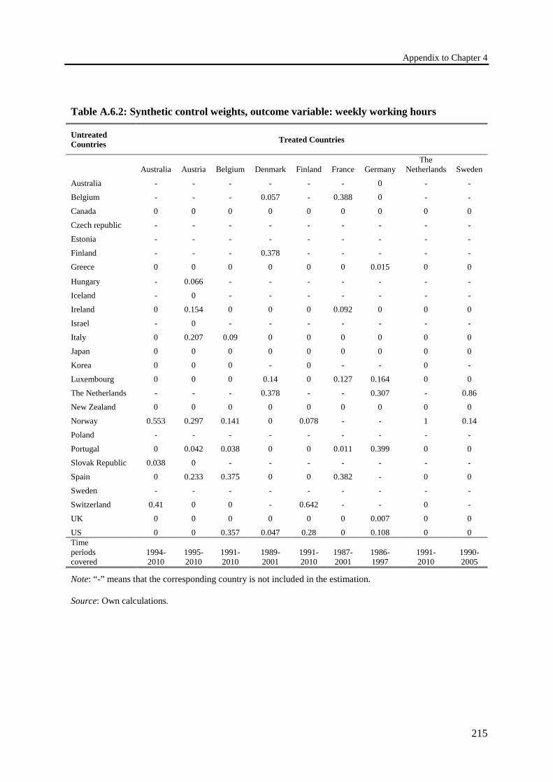
Appendix to Chapter 4
215
Table A.6.2: Synthetic control weights, outcome variable: weekly working hours
Untreated Countries Treated Countries
Australia Austria Belgium Denmark Finland France Germany The
Netherlands Sweden
Australia - - - - - - 0 - -
Belgium - - - 0.057 - 0.388 0 - -
Canada 0 0 0 0 0 0 0 0 0
Czech republic - - - - - - - - -
Estonia - - - - - - - - -
Finland - - - 0.378 - - - - -
Greece 0 0 0 0 0 0 0.015 0 0
Hungary - 0.066 - - - - - - -
Iceland - 0 - - - - - - -
Ireland 0 0.154 0 0 0 0.092 0 0 0
Israel - 0 - - - - - - -
Italy 0 0.207 0.09 0 0 0 0 0 0
Japan 0 0 0 0 0 0 0 0 0
Korea 0 0 0 - 0 - - 0 -
Luxembourg 0 0 0 0.14 0 0.127 0.164 0 0
The Netherlands - - - 0.378 - - 0.307 - 0.86
New Zealand 0 0 0 0 0 0 0 0 0
Norway 0.553 0.297 0.141 0 0.078 - - 1 0.14
Poland - - - - - - - - -
Portugal 0 0.042 0.038 0 0 0.011 0.399 0 0
Slovak Republic 0.038 0 - - - - - - -
Spain 0 0.233 0.375 0 0 0.382 - 0 0
Sweden - - - - - - - - -
Switzerland 0.41 0 0 - 0.642 - - 0 -
UK 0 0 0 0 0 0 0.007 0 0
US 0 0 0.357 0.047 0.28 0 0.108 0 0 Time periods covered
1994- 2010
1995- 2010
1991- 2010
1989- 2001
1991- 2010
1987- 2001
1986- 1997
1991- 2010
1990- 2005
Note: “-” means that the corresponding country is not included in the estimation.
Source: Own calculations.
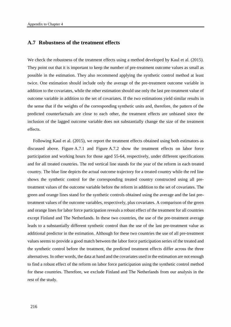
Appendix to Chapter 4
216
A.7 Robustness of the treatment effects
We check the robustness of the treatment effects using a method developed by Kaul et al. (2015).
They point out that it is important to keep the number of pre-treatment outcome values as small as
possible in the estimation. They also recommend applying the synthetic control method at least
twice. One estimation should include only the average of the pre-treatment outcome variable in
addition to the covariates, while the other estimation should use only the last pre-treatment value of
outcome variable in addition to the set of covariates. If the two estimations yield similar results in
the sense that if the weights of the corresponding synthetic units and, therefore, the pattern of the
predicted counterfactuals are close to each other, the treatment effects are unbiased since the
inclusion of the lagged outcome variable does not substantially change the size of the treatment
effects.
Following Kaul et al. (2015), we report the treatment effects obtained using both estimators as
discussed above. Figure A.7.1 and Figure A.7.2 show the treatment effects on labor force
participation and working hours for those aged 55-64, respectively, under different specifications
and for all treated countries. The red vertical line stands for the year of the reform in each treated
country. The blue line depicts the actual outcome trajectory for a treated country while the red line
shows the synthetic control for the corresponding treated country constructed using all pre-
treatment values of the outcome variable before the reform in addition to the set of covariates. The
green and orange lines stand for the synthetic controls obtained using the average and the last pre-
treatment values of the outcome variables, respectively, plus covariates. A comparison of the green
and orange lines for labor force participation reveals a robust effect of the treatment for all countries
except Finland and The Netherlands. In these two countries, the use of the pre-treatment average
leads to a substantially different synthetic control than the use of the last pre-treatment value as
additional predictor in the estimation. Although for these two countries the use of all pre-treatment
values seems to provide a good match between the labor force participation series of the treated and
the synthetic control before the treatment, the predicted treatment effects differ across the three
alternatives. In other words, the data at hand and the covariates used in the estimation are not enough
to find a robust effect of the reform on labor force participation using the synthetic control method
for these countries. Therefore, we exclude Finland and The Netherlands from our analysis in the
rest of the study.
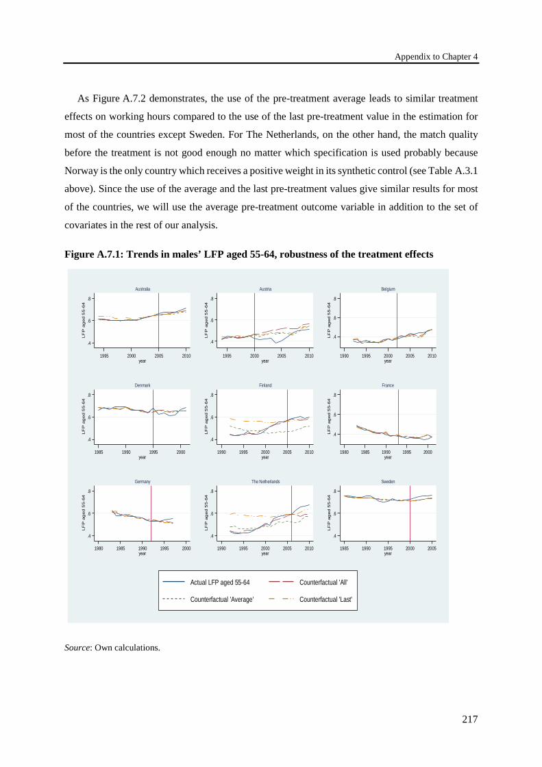
Appendix to Chapter 4
217
As Figure A.7.2 demonstrates, the use of the pre-treatment average leads to similar treatment
effects on working hours compared to the use of the last pre-treatment value in the estimation for
most of the countries except Sweden. For The Netherlands, on the other hand, the match quality
before the treatment is not good enough no matter which specification is used probably because
Norway is the only country which receives a positive weight in its synthetic control (see Table A.3.1
above). Since the use of the average and the last pre-treatment values give similar results for most
of the countries, we will use the average pre-treatment outcome variable in addition to the set of
covariates in the rest of our analysis.
Figure A.7.1: Trends in males’ LFP aged 55-64, robustness of the treatment effects
Source: Own calculations.
.4
.6
.8
LFP
ag
ed 5
5-64
1995 2000 2005 2010year
Australia
.4
.6
.8
LFP
ag
ed 5
5-64
1995 2000 2005 2010year
Austria
.4
.6
.8
LFP
ag
ed 5
5-64
1990 1995 2000 2005 2010year
Belgium
.4
.6
.8
LFP
ag
ed 5
5-64
1985 1990 1995 2000year
Denmark
.4
.6
.8
LFP
ag
ed 5
5-64
1990 1995 2000 2005 2010year
Finland
.4
.6
.8
LFP
ag
ed 5
5-64
1980 1985 1990 1995 2000year
France
.4
.6
.8
LFP
ag
ed 5
5-64
1980 1985 1990 1995 2000year
Germany
.4
.6
.8
LFP
ag
ed 5
5-64
1990 1995 2000 2005 2010year
The Netherlands
.4
.6
.8
LFP
ag
ed 5
5-64
1985 1990 1995 2000 2005year
Sweden
Actual LFP aged 55-64 Counterfactual 'All'
Counterfactual 'Average' Counterfactual 'Last'
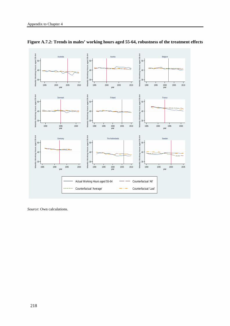
Appendix to Chapter 4
218
Figure A.7.2: Trends in males’ working hours aged 55-64, robustness of the treatment effects
Source: Own calculations.
30
40
50
Wee
kly
Wo
rkin
g H
ours
age
d 55
-64
1995 2000 2005 2010year
Australia
30
40
50
Wee
kly
Wo
rkin
g H
ours
age
d 55
-64
1995 2000 2005 2010year
Austria
30
40
50
Wee
kly
Wo
rkin
g H
ours
age
d 55
-64
1990 1995 2000 2005 2010year
Belgium
30
40
50
Wee
kly
Wo
rkin
g H
ours
age
d 55
-64
1990 1995 2000year
Denmark
30
40
50
Wee
kly
Wo
rkin
g H
ours
age
d 55
-64
1990 1995 2000 2005 2010year
Finland
30
40
50
Wee
kly
Wo
rkin
g H
ours
age
d 55
-64
1985 1990 1995 2000year
France
30
40
50
Wee
kly
Wo
rkin
g H
ours
age
d 55
-64
1985 1990 1995 2000year
Germany
30
40
50
Wee
kly
Wo
rkin
g H
ours
age
d 55
-64
1990 1995 2000 2005 2010year
The Netherlands
30
40
50W
eekl
y W
ork
ing
Hou
rs a
ged
55-6
4
1990 1995 2000 2005year
Sweden
Actual Working Hours aged 55-64 Counterfactual 'All'
Counterfactual 'Average' Counterfactual 'Last'
Appendix to Chapter 4
219
A.8 The quality of pre-treatment characteristics
Table A.8.1 and Table A.8.2 compare the pre-treatment characteristics of the synthetic control to
those of the treated country where the outcome variables are labor force participation and working
hours, respectively. Overall, the results suggest that for all countries which adopted a flexibility
reform in the past, the synthetic country provides a good approximation for the corresponding actual
country before the reform. Only in few cases, there is a discrepancy between the treated country
and its synthetic control in terms of GDP per capita. This stems from the fact that among all
predictor variables GDP per capita has the lowest power especially for predicting labor force
participation before the reform. For some countries we used the standard retirement age instead of
the possible years of early retirement as the quality of the pre-treatment matches increased
remarkably in those cases.
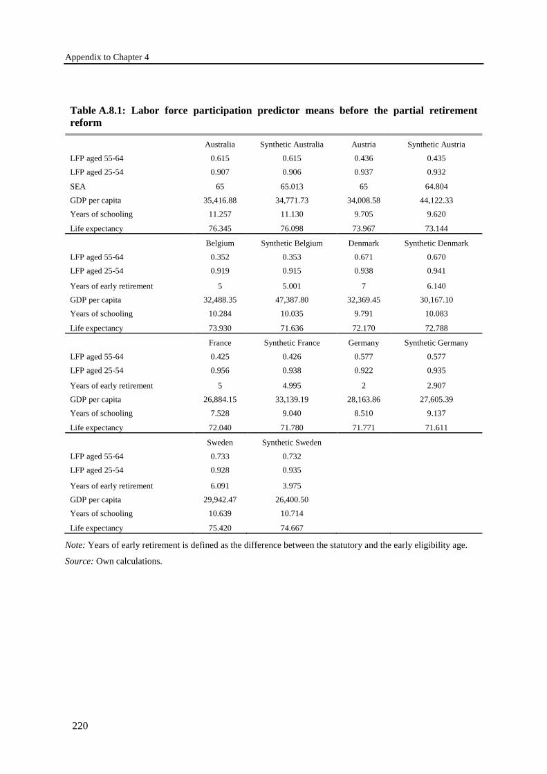
Appendix to Chapter 4
220
Table A.8.1: Labor force participation predictor means before the partial retirement reform
Australia Synthetic Australia Austria Synthetic Austria
LFP aged 55-64 0.615 0.615 0.436 0.435
LFP aged 25-54 0.907 0.906 0.937 0.932
SEA 65 65.013 65 64.804
GDP per capita 35,416.88 34,771.73 34,008.58 44,122.33
Years of schooling 11.257 11.130 9.705 9.620
Life expectancy 76.345 76.098 73.967 73.144
Belgium Synthetic Belgium Denmark Synthetic Denmark
LFP aged 55-64 0.352 0.353 0.671 0.670
LFP aged 25-54 0.919 0.915 0.938 0.941
Years of early retirement 5 5.001 7 6.140
GDP per capita 32,488.35 47,387.80 32,369.45 30,167.10
Years of schooling 10.284 10.035 9.791 10.083
Life expectancy 73.930 71.636 72.170 72.788
France Synthetic France Germany Synthetic Germany
LFP aged 55-64 0.425 0.426 0.577 0.577
LFP aged 25-54 0.956 0.938 0.922 0.935
Years of early retirement 5 4.995 2 2.907
GDP per capita 26,884.15 33,139.19 28,163.86 27,605.39
Years of schooling 7.528 9.040 8.510 9.137
Life expectancy 72.040 71.780 71.771 71.611
Sweden Synthetic Sweden LFP aged 55-64 0.733 0.732 LFP aged 25-54 0.928 0.935
Years of early retirement 6.091 3.975 GDP per capita 29,942.47 26,400.50 Years of schooling 10.639 10.714 Life expectancy 75.420 74.667
Note: Years of early retirement is defined as the difference between the statutory and the early eligibility age.
Source: Own calculations.
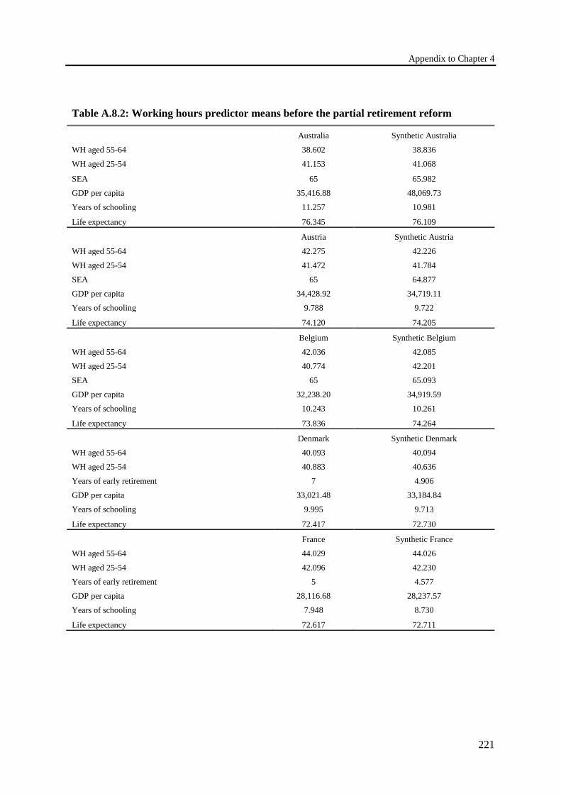
Appendix to Chapter 4
221
Table A.8.2: Working hours predictor means before the partial retirement reform
Australia Synthetic Australia
WH aged 55-64 38.602 38.836
WH aged 25-54 41.153 41.068
SEA 65 65.982
GDP per capita 35,416.88 48,069.73
Years of schooling 11.257 10.981
Life expectancy 76.345 76.109
Austria Synthetic Austria
WH aged 55-64 42.275 42.226
WH aged 25-54 41.472 41.784
SEA 65 64.877
GDP per capita 34,428.92 34,719.11
Years of schooling 9.788 9.722
Life expectancy 74.120 74.205
Belgium Synthetic Belgium
WH aged 55-64 42.036 42.085
WH aged 25-54 40.774 42.201
SEA 65 65.093
GDP per capita 32,238.20 34,919.59
Years of schooling 10.243 10.261
Life expectancy 73.836 74.264
Denmark Synthetic Denmark
WH aged 55-64 40.093 40.094
WH aged 25-54 40.883 40.636
Years of early retirement 7 4.906
GDP per capita 33,021.48 33,184.84
Years of schooling 9.995 9.713
Life expectancy 72.417 72.730
France Synthetic France
WH aged 55-64 44.029 44.026
WH aged 25-54 42.096 42.230
Years of early retirement 5 4.577
GDP per capita 28,116.68 28,237.57
Years of schooling 7.948 8.730
Life expectancy 72.617 72.711

Appendix to Chapter 4
222
Germany Synthetic Germany WH aged 55-64 43.265 43.266 WH aged 25-54 42.088 42.596 Years of early retirement 2 2.581 GDP per capita 29,266.27 28,739.65 Years of schooling 8.810 8.791 Life expectancy 71.883 71.757
Note: Years of early retirement is defined as the difference between the statutory and the early eligibility age.
Source: Own calculations.
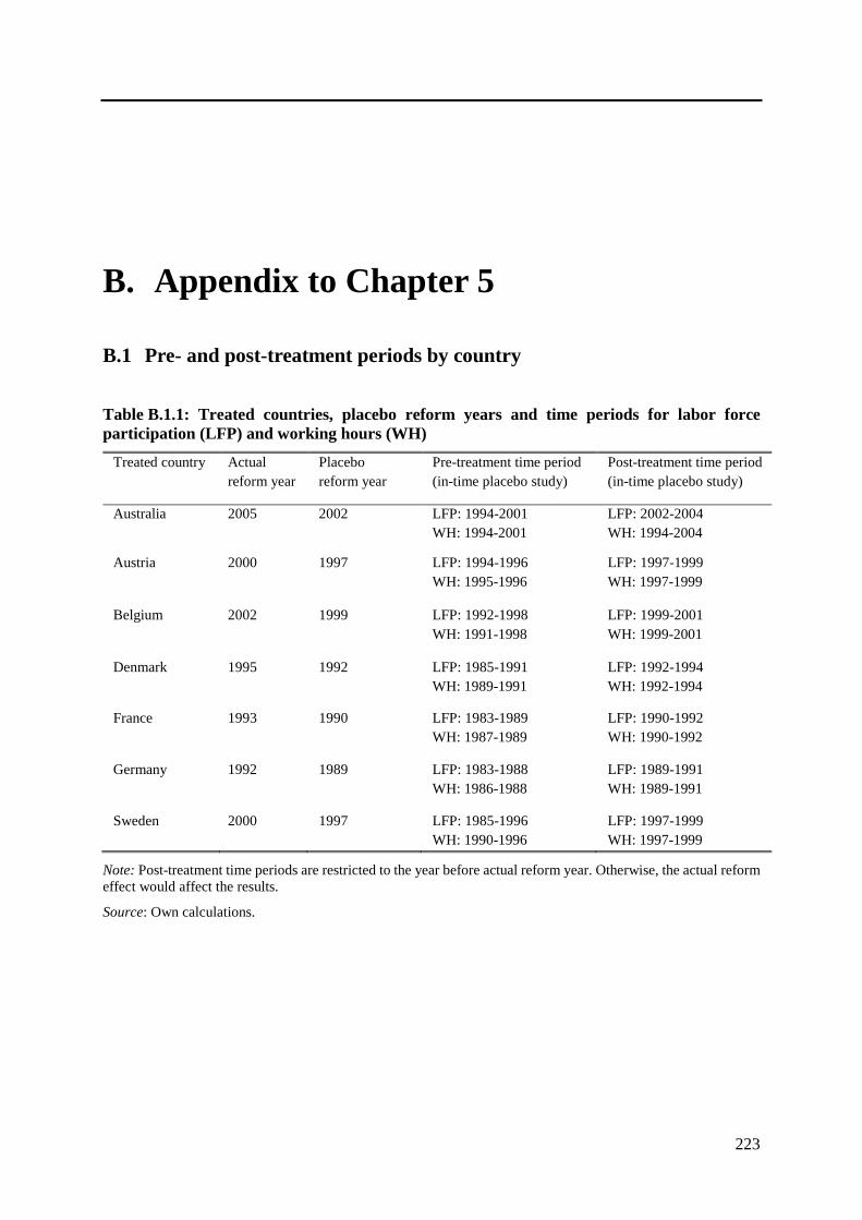
223
B. Appendix to Chapter 5
B.1 Pre- and post-treatment periods by country
Table B.1.1: Treated countries, placebo reform years and time periods for labor force participation (LFP) and working hours (WH)
Treated country Actual reform year
Placebo reform year
Pre-treatment time period (in-time placebo study)
Post-treatment time period (in-time placebo study)
Australia 2005 2002 LFP: 1994-2001 WH: 1994-2001
LFP: 2002-2004 WH: 1994-2004
Austria 2000 1997 LFP: 1994-1996 WH: 1995-1996
LFP: 1997-1999 WH: 1997-1999
Belgium 2002 1999 LFP: 1992-1998 WH: 1991-1998
LFP: 1999-2001 WH: 1999-2001
Denmark 1995 1992 LFP: 1985-1991 WH: 1989-1991
LFP: 1992-1994 WH: 1992-1994
France 1993 1990 LFP: 1983-1989 WH: 1987-1989
LFP: 1990-1992 WH: 1990-1992
Germany 1992 1989 LFP: 1983-1988 WH: 1986-1988
LFP: 1989-1991 WH: 1989-1991
Sweden 2000 1997 LFP: 1985-1996 WH: 1990-1996
LFP: 1997-1999 WH: 1997-1999
Note: Post-treatment time periods are restricted to the year before actual reform year. Otherwise, the actual reform effect would affect the results.
Source: Own calculations.
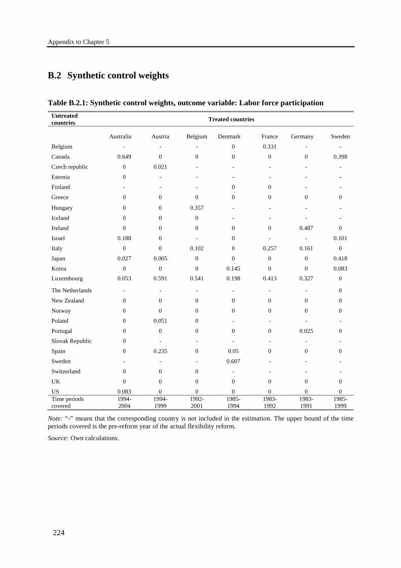
Appendix to Chapter 5
224
B.2 Synthetic control weights
Table B.2.1: Synthetic control weights, outcome variable: Labor force participation Untreated countries Treated countries
Australia Austria Belgium Denmark France Germany Sweden
Belgium - - - 0 0.331 - -
Canada 0.649 0 0 0 0 0 0.398
Czech republic 0 0.021 - - - - -
Estonia 0 - - - - - -
Finland - - - 0 0 - -
Greece 0 0 0 0 0 0 0
Hungary 0 0 0.357 - - - -
Iceland 0 0 0 - - - -
Ireland 0 0 0 0 0 0.487 0
Israel 0.188 0 - 0 - - 0.101
Italy 0 0 0.102 0 0.257 0.161 0
Japan 0.027 0.005 0 0 0 0 0.418
Korea 0 0 0 0.145 0 0 0.083 Luxembourg 0.053 0.591 0.541 0.198 0.413 0.327 0
The Netherlands - - - - - - 0
New Zealand 0 0 0 0 0 0 0
Norway 0 0 0 0 0 0 0
Poland 0 0.051 0 - - - -
Portugal 0 0 0 0 0 0.025 0 Slovak Republic 0 - - - - - -
Spain 0 0.235 0 0.05 0 0 0
Sweden - - - 0.607 - - -
Switzerland 0 0 0 - - - -
UK 0 0 0 0 0 0 0
US 0.083 0 0 0 0 0 0 Time periods covered
1994- 2004
1994- 1999
1992- 2001
1985- 1994
1983- 1992
1983- 1991
1985- 1999
Note: “-” means that the corresponding country is not included in the estimation. The upper bound of the time periods covered is the pre-reform year of the actual flexibility reform.
Source: Own calculations.
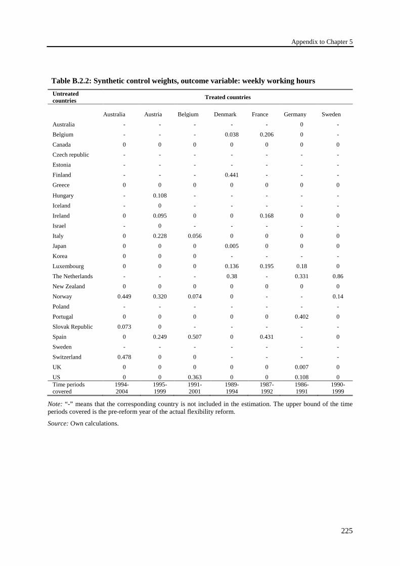
Appendix to Chapter 5
225
Table B.2.2: Synthetic control weights, outcome variable: weekly working hours Untreated countries Treated countries
Australia Austria Belgium Denmark France Germany Sweden
Australia - - - - - 0 -
Belgium - - - 0.038 0.206 0 -
Canada 0 0 0 0 0 0 0
Czech republic - - - - - - -
Estonia - - - - - - -
Finland - - - 0.441 - - -
Greece 0 0 0 0 0 0 0
Hungary - 0.108 - - - - -
Iceland - 0 - - - - -
Ireland 0 0.095 0 0 0.168 0 0
Israel - 0 - - - - -
Italy 0 0.228 0.056 0 0 0 0
Japan 0 0 0 0.005 0 0 0
Korea 0 0 0 - - - -
Luxembourg 0 0 0 0.136 0.195 0.18 0
The Netherlands - - - 0.38 - 0.331 0.86
New Zealand 0 0 0 0 0 0 0
Norway 0.449 0.320 0.074 0 - - 0.14
Poland - - - - - - -
Portugal 0 0 0 0 0 0.402 0
Slovak Republic 0.073 0 - - - - -
Spain 0 0.249 0.507 0 0.431 - 0
Sweden - - - - - - -
Switzerland 0.478 0 0 - - - -
UK 0 0 0 0 0 0.007 0
US 0 0 0.363 0 0 0.108 0 Time periods covered
1994- 2004
1995- 1999
1991- 2001
1989- 1994
1987- 1992
1986- 1991
1990- 1999
Note: “-” means that the corresponding country is not included in the estimation. The upper bound of the time periods covered is the pre-reform year of the actual flexibility reform.
Source: Own calculations.
Appendix to Chapter 5
226
B.3 Robustness of the treatment effects
As in Chapter 4, I check the robustness of the treatment effects for the case of the placebo reform
years by using a method developed by Kaul et al. (2015, updated in Kaul et al. 2018). Kaul et al.
(2015) recommend applying the synthetic control method at least twice: one estimation should
incorporate only the average of the outcome variable’s pre-treatment values in addition to the set of
covariates. Another version should only include the last pre-treatment value of the outcome variable
(i.e. in the last period before the treatment) in addition to the other covariates. If the two estimation
versions yield similar results in terms of similar weights of the corresponding synthetic units and,
therefore, in terms of similar patterns of the predicted counterfactuals that come close to each other,
the treatment effects are unbiased.
Another specification could include all pre-treatment values in addition to the covariates. Kaul et
al. (2018) state that it actually becomes increasingly popular in applications of synthetic control
methods to include the entire pre-treatment path of the outcome variable as economic predictors
and following Cavallo et al. (2013) including the entire pre-treatment path seems the obvious
choice. Including all pre-treatment values of the outcome variables is exactly was has been done,
e.g., in Bilgel and Galle (2015), Billmeier and Nannicini (2013), Bohn et al. (2014), Hinrichs
(2012), Kreif et al. (2016), Liu (2015), Nannicini and Billmeier (2011), O’Neill et al. (2016), and
Stearns (2015). Kaul et al. (2018) demonstrate, however, both theoretically and empirically that
incorporating all outcome lags causes all other covariates to be irrelevant in the estimation. This
finding holds irrespective of how important these covariates are for accurately predicting post-
treatment values of the outcome and therefore threatens the estimator’s unbiasedness.
Following the recommendation of Kaul et al. (2015) to apply the synthetic control method at least
twice, I report treatment effects on labor force participation (Figure B.3.1) and working hours
(Figure B.3.2) for males aged 55-64, under different specifications and for all treated countries. In
Figure B.3.1 and Figure B.3.2, the red vertical line indicates the placebo reform year. The blue solid
line depicts the actual outcome trajectory of the treated country and the red long dashed-dotted line
shows the synthetic control country when controlling for the entire pre-treatment path of the
outcome variable (“All”) in addition to the set of other covariates. While the green dashed line
represents the synthetic control when including the average pre-treatment value of the outcome
variable plus covariates, the orange short dashed-dotted line depicts the specification when
controlling for the last pre-treatment outcome value only plus covariates. The comparison of the
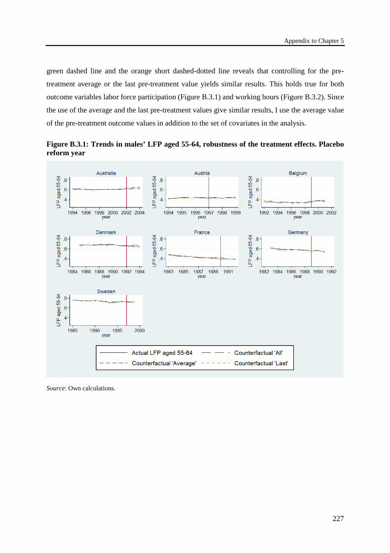
Appendix to Chapter 5
227
green dashed line and the orange short dashed-dotted line reveals that controlling for the pre-
treatment average or the last pre-treatment value yields similar results. This holds true for both
outcome variables labor force participation (Figure B.3.1) and working hours (Figure B.3.2). Since
the use of the average and the last pre-treatment values give similar results, I use the average value
of the pre-treatment outcome values in addition to the set of covariates in the analysis.
Figure B.3.1: Trends in males’ LFP aged 55-64, robustness of the treatment effects. Placebo reform year
Source: Own calculations.
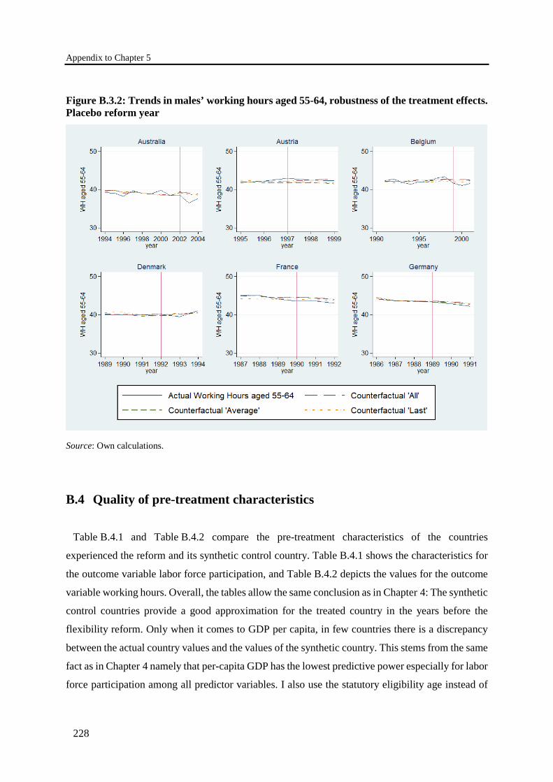
Appendix to Chapter 5
228
Figure B.3.2: Trends in males’ working hours aged 55-64, robustness of the treatment effects. Placebo reform year
Source: Own calculations.
B.4 Quality of pre-treatment characteristics
Table B.4.1 and Table B.4.2 compare the pre-treatment characteristics of the countries
experienced the reform and its synthetic control country. Table B.4.1 shows the characteristics for
the outcome variable labor force participation, and Table B.4.2 depicts the values for the outcome
variable working hours. Overall, the tables allow the same conclusion as in Chapter 4: The synthetic
control countries provide a good approximation for the treated country in the years before the
flexibility reform. Only when it comes to GDP per capita, in few countries there is a discrepancy
between the actual country values and the values of the synthetic country. This stems from the same
fact as in Chapter 4 namely that per-capita GDP has the lowest predictive power especially for labor
force participation among all predictor variables. I also use the statutory eligibility age instead of
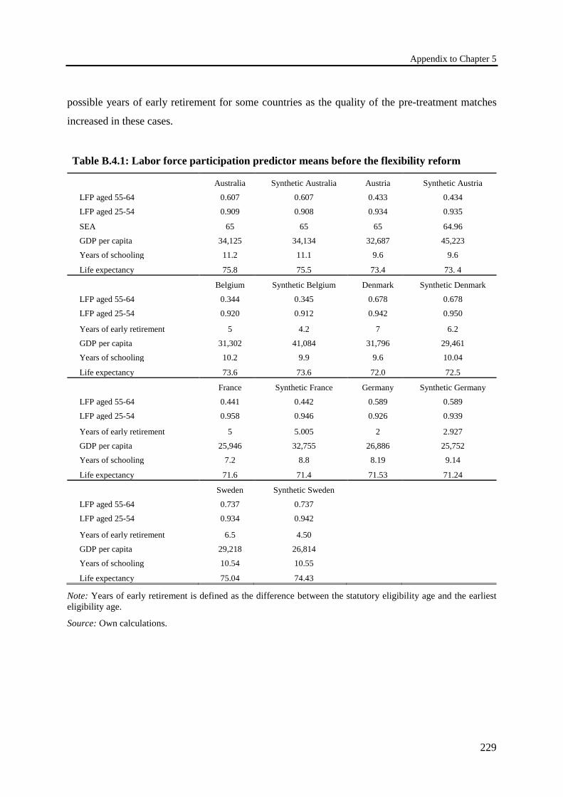
Appendix to Chapter 5
229
possible years of early retirement for some countries as the quality of the pre-treatment matches
increased in these cases.
Table B.4.1: Labor force participation predictor means before the flexibility reform
Australia Synthetic Australia Austria Synthetic Austria
LFP aged 55-64 0.607 0.607 0.433 0.434
LFP aged 25-54 0.909 0.908 0.934 0.935
SEA 65 65 65 64.96
GDP per capita 34,125 34,134 32,687 45,223
Years of schooling 11.2 11.1 9.6 9.6
Life expectancy 75.8 75.5 73.4 73. 4
Belgium Synthetic Belgium Denmark Synthetic Denmark
LFP aged 55-64 0.344 0.345 0.678 0.678
LFP aged 25-54 0.920 0.912 0.942 0.950
Years of early retirement 5 4.2 7 6.2
GDP per capita 31,302 41,084 31,796 29,461
Years of schooling 10.2 9.9 9.6 10.04
Life expectancy 73.6 73.6 72.0 72.5
France Synthetic France Germany Synthetic Germany
LFP aged 55-64 0.441 0.442 0.589 0.589
LFP aged 25-54 0.958 0.946 0.926 0.939
Years of early retirement 5 5.005 2 2.927
GDP per capita 25,946 32,755 26,886 25,752
Years of schooling 7.2 8.8 8.19 9.14
Life expectancy 71.6 71.4 71.53 71.24
Sweden Synthetic Sweden LFP aged 55-64 0.737 0.737 LFP aged 25-54 0.934 0.942
Years of early retirement 6.5 4.50 GDP per capita 29,218 26,814 Years of schooling 10.54 10.55 Life expectancy 75.04 74.43
Note: Years of early retirement is defined as the difference between the statutory eligibility age and the earliest eligibility age.
Source: Own calculations.
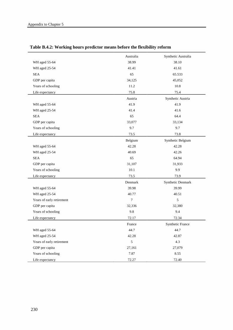
Appendix to Chapter 5
230
Table B.4.2: Working hours predictor means before the flexibility reform
Australia Synthetic Australia
WH aged 55-64 38.99 38.10
WH aged 25-54 41.41 41.61
SEA 65 65.533
GDP per capita 34,125 45,052
Years of schooling 11.2 10.8
Life expectancy 75.8 75.4
Austria Synthetic Austria
WH aged 55-64 41.9 41.9
WH aged 25-54 41.4 41.6
SEA 65 64.4
GDP per capita 33,077 33,134
Years of schooling 9.7 9.7
Life expectancy 73.5 73.8
Belgium Synthetic Belgium
WH aged 55-64 42.28 42.28
WH aged 25-54 40.69 42.26
SEA 65 64.94
GDP per capita 31,107 31,933
Years of schooling 10.1 9.9
Life expectancy 73.5 73.9
Denmark Synthetic Denmark
WH aged 55-64 39.98 39.99
WH aged 25-54 40.77 40.51
Years of early retirement 7 5
GDP per capita 32,336 32,380
Years of schooling 9.8 9.4
Life expectancy 72.17 72.34
France Synthetic France
WH aged 55-64 44.7 44.7
WH aged 25-54 42.28 42.87
Years of early retirement 5 4.3
GDP per capita 27,161 27,079
Years of schooling 7.87 8.55
Life expectancy 72.27 72.40
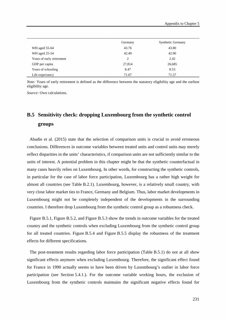
Appendix to Chapter 5
231
Germany Synthetic Germany
WH aged 55-64 43.76 43.80 WH aged 25-54 42.49 42.90 Years of early retirement 2 2.42 GDP per capita 27,814 26,685 Years of schooling 8.47 8.53 Life expectancy 71.67 71.57
Note: Years of early retirement is defined as the difference between the statutory eligibility age and the earliest eligibility age.
Source: Own calculations.
B.5 Sensitivity check: dropping Luxembourg from the synthetic control
groups
Abadie et al. (2015) state that the selection of comparison units is crucial to avoid erroneous
conclusions. Differences in outcome variables between treated units and control units may merely
reflect disparities in the units’ characteristics, if comparison units are not sufficiently similar to the
units of interest. A potential problem in this chapter might be that the synthetic counterfactual in
many cases heavily relies on Luxembourg. In other words, for constructing the synthetic controls,
in particular for the case of labor force participation, Luxembourg has a rather high weight for
almost all countries (see Table B.2.1). Luxembourg, however, is a relatively small country, with
very close labor market ties to France, Germany and Belgium. Thus, labor market developments in
Luxembourg might not be completely independent of the developments in the surrounding
countries. I therefore drop Luxembourg from the synthetic control group as a robustness check.
Figure B.5.1, Figure B.5.2, and Figure B.5.3 show the trends in outcome variables for the treated
country and the synthetic controls when excluding Luxembourg from the synthetic control group
for all treated countries. Figure B.5.4 and Figure B.5.5 display the robustness of the treatment
effects for different specifications.
The post-treatment results regarding labor force participation (Table B.5.1) do not at all show
significant effects anymore when excluding Luxembourg. Therefore, the significant effect found
for France in 1990 actually seems to have been driven by Luxembourg’s outlier in labor force
participation (see Section 5.4.1.). For the outcome variable working hours, the exclusion of
Luxembourg from the synthetic controls maintains the significant negative effects found for
Appendix to Chapter 5
232
Australia (2003) and France (1990) (see Section 5.4.2.). For France, this most likely stems from a
poor synthetic control. Due to data availability, the pre-treatment period is only three years and does
constitute a solid basis to develop a stable synthetic control. However, the effect for Australia may
be due to a set of reforms of the superannuation system that happened in 2002 and 2003 (see
Section 5.4.2. and Section 5.4.3.). Both effects persist when excluding Luxembourg from the
synthetic controls. Excluding Luxembourg from the synthetic controls yields significant negative
effects on working hours for Germany (1989, 1990, 1991). The effects for Germany, however, very
likely stem from a reform which first came into effect in 1989 and initialized part-time employment
before retirement (Altersteilzeit). This scheme comprised a reduction of working hours in a specific
period before full retirement (Lindecke et al. 2017). In practice, the scheme achieved its
breakthrough only after a revision in the later 1990s, but may explain the negative effects found on
working hours. While the negative effect for Australia (2003) translates also to total labor supply
(Table B.5.3), no other effects remain significant. Overall, the robustness check excluding
Luxembourg suggest that the results are not driven by the inclusion of Luxembourg in the synthetic
controls.
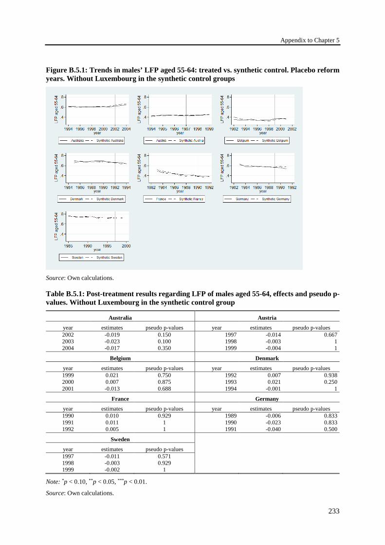
Appendix to Chapter 5
233
Figure B.5.1: Trends in males’ LFP aged 55-64: treated vs. synthetic control. Placebo reform years. Without Luxembourg in the synthetic control groups
Source: Own calculations.
Table B.5.1: Post-treatment results regarding LFP of males aged 55-64, effects and pseudo p-values. Without Luxembourg in the synthetic control group
Australia Austria
year estimates pseudo p-values year estimates pseudo p-values 2002 -0.019 0.150 1997 -0.014 0.667 2003 -0.023 0.100 1998 -0.003 1 2004 -0.017 0.350 1999 -0.004 1
Belgium Denmark
year estimates pseudo p-values year estimates pseudo p-values 1999 0.021 0.750 1992 0.007 0.938 2000 0.007 0.875 1993 0.021 0.250 2001 -0.013 0.688 1994 -0.001 1
France Germany
year estimates pseudo p-values year estimates pseudo p-values 1990 0.010 0.929 1989 -0.006 0.833 1991 0.011 1 1990 -0.023 0.833 1992 0.005 1 1991 -0.040 0.500
Sweden
year estimates pseudo p-values 1997 -0.011 0.571 1998 -0.003 0.929 1999 -0.002 1
Note: *p < 0.10, **p < 0.05, ***p < 0.01.
Source: Own calculations.
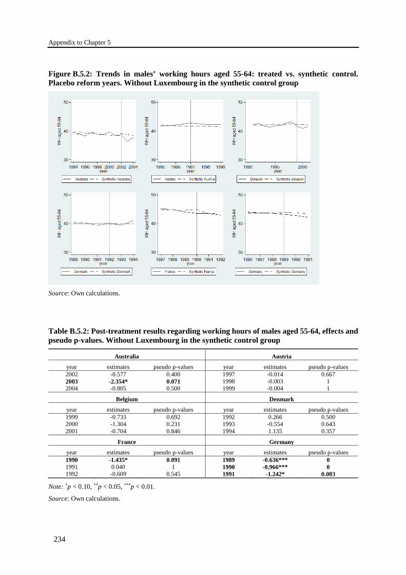
Appendix to Chapter 5
234
Figure B.5.2: Trends in males’ working hours aged 55-64: treated vs. synthetic control. Placebo reform years. Without Luxembourg in the synthetic control group
Source: Own calculations.
Table B.5.2: Post-treatment results regarding working hours of males aged 55-64, effects and pseudo p-values. Without Luxembourg in the synthetic control group
Australia Austria
year estimates pseudo p-values year estimates pseudo p-values 2002 -0.577 0.400 1997 -0.014 0.667 2003 -2.354* 0.071 1998 -0.003 1 2004 -0.805 0.500 1999 -0.004 1
Belgium Denmark
year estimates pseudo p-values year estimates pseudo p-values 1999 -0.733 0.692 1992 0.266 0.500 2000 -1.304 0.231 1993 -0.554 0.643 2001 -0.704 0.846 1994 1.135 0.357
France Germany
year estimates pseudo p-values year estimates pseudo p-values 1990 -1.435* 0.091 1989 -0.636*** 0 1991 0.040 1 1990 -0.966*** 0 1992 -0.609 0.545 1991 -1.242* 0.083
Note: *p < 0.10, **p < 0.05, ***p < 0.01.
Source: Own calculations.
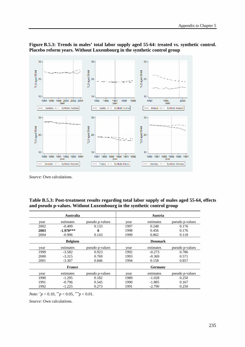
Appendix to Chapter 5
235
Figure B.5.3: Trends in males’ total labor supply aged 55-64: treated vs. synthetic control. Placebo reform years. Without Luxembourg in the synthetic control group
Source: Own calculations.
Table B.5.3: Post-treatment results regarding total labor supply of males aged 55-64, effects and pseudo p-values. Without Luxembourg in the synthetic control group
Australia Austria
year estimates pseudo p-values year estimates pseudo p-values 2002 -0.409 0.133 1997 0.248 0.176 2003 -1.970*** 0 1998 0.456 0.176 2004 -0.996 0.143 1999 0.862 0.118
Belgium Denmark
year estimates pseudo p-values year estimates pseudo p-values 1999 -3.582 0.923 1992 -0.273 0.786 2000 -3.315 0.769 1993 -0.369 0.571 2001 -3.307 0.846 1994 0.158 0.857
France Germany
year estimates pseudo p-values year estimates pseudo p-values 1990 -1.295 0.182 1989 -1.028 0.250 1991 -0.796 0.545 1990 -1.885 0.167 1992 -1.225 0.273 1991 -2.790 0.250
Note: *p < 0.10, **p < 0.05, ***p < 0.01.
Source: Own calculations.
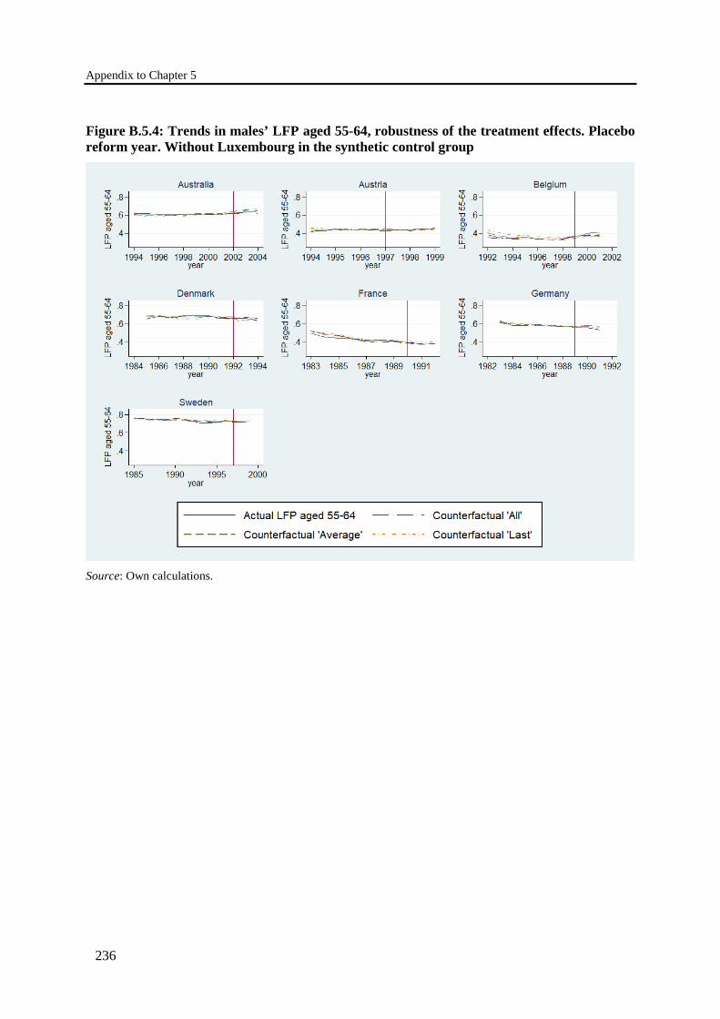
Appendix to Chapter 5
236
Figure B.5.4: Trends in males’ LFP aged 55-64, robustness of the treatment effects. Placebo reform year. Without Luxembourg in the synthetic control group
Source: Own calculations.
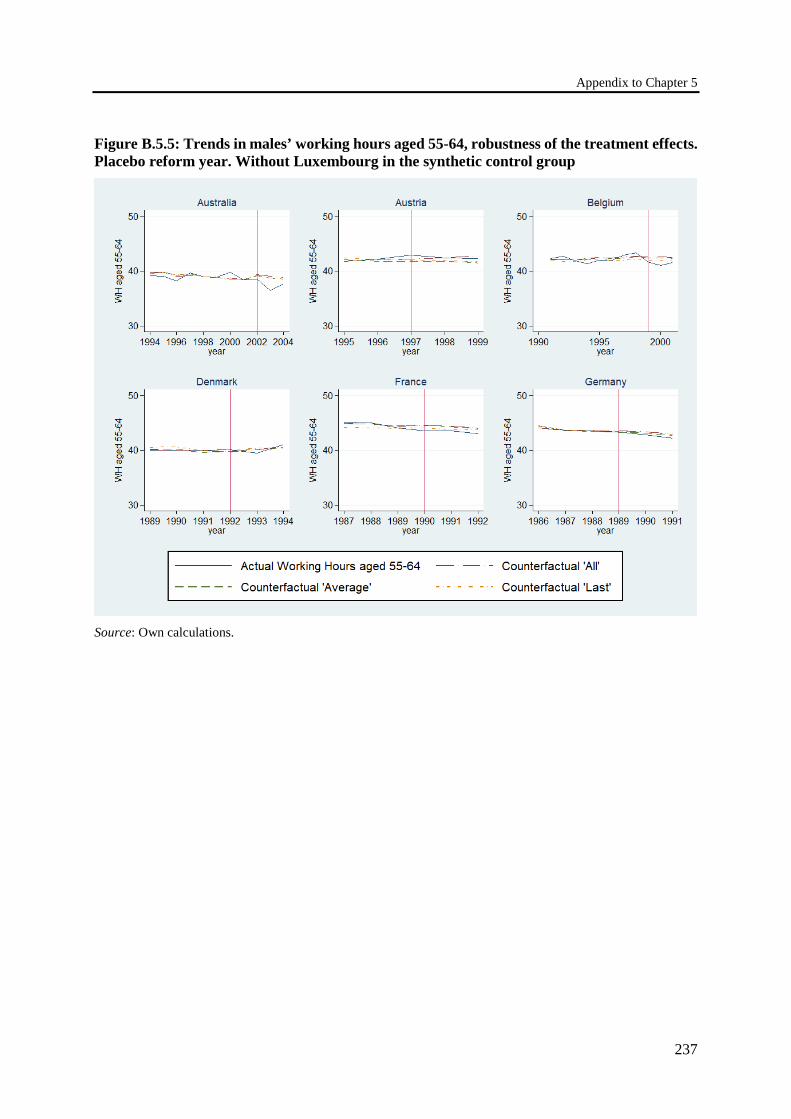
Appendix to Chapter 5
237
Figure B.5.5: Trends in males’ working hours aged 55-64, robustness of the treatment effects. Placebo reform year. Without Luxembourg in the synthetic control group
Source: Own calculations.
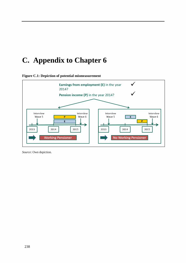
238
C. Appendix to Chapter 6
Figure C.1: Depiction of potential mismeasurement
Source: Own depiction.
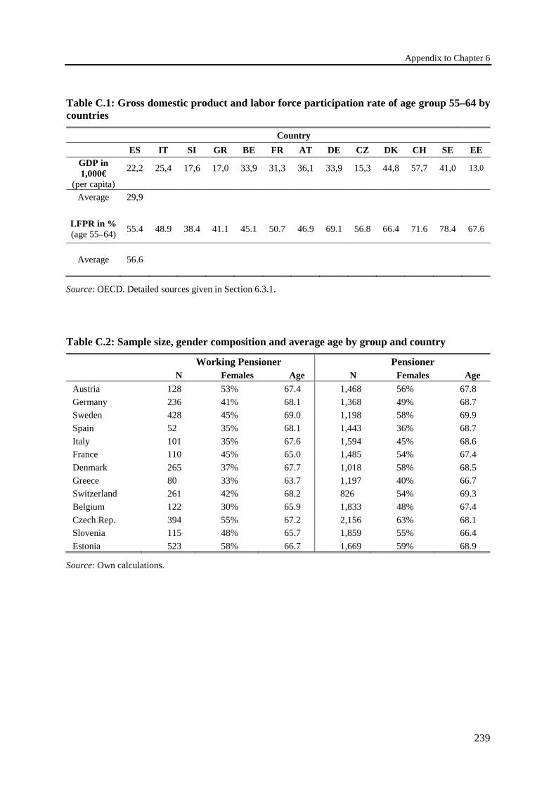
Appendix to Chapter 6
239
Table C.1: Gross domestic product and labor force participation rate of age group 55–64 by countries
Country ES IT SI GR BE FR AT DE CZ DK CH SE EE
GDP in 1,000€
(per capita)
22,2
25,4
17,6
17,0
33,9
31,3
36,1
33,9
15,3
44,8
57,7
41,0
13,0
Average 29,9
LFPR in % (age 55–64) 55.4 48.9 38.4 41.1 45.1 50.7 46.9 69.1 56.8 66.4 71.6 78.4 67.6
Average
56.6
Source: OECD. Detailed sources given in Section 6.3.1.
Table C.2: Sample size, gender composition and average age by group and country
Working Pensioner Pensioner N Females Age N Females Age
Austria 128 53% 67.4 1,468 56% 67.8 Germany 236 41% 68.1 1,368 49% 68.7 Sweden 428 45% 69.0 1,198 58% 69.9 Spain 52 35% 68.1 1,443 36% 68.7 Italy 101 35% 67.6 1,594 45% 68.6 France 110 45% 65.0 1,485 54% 67.4 Denmark 265 37% 67.7 1,018 58% 68.5 Greece 80 33% 63.7 1,197 40% 66.7 Switzerland 261 42% 68.2 826 54% 69.3 Belgium 122 30% 65.9 1,833 48% 67.4 Czech Rep. 394 55% 67.2 2,156 63% 68.1 Slovenia 115 48% 65.7 1,859 55% 66.4 Estonia 523 58% 66.7 1,669 59% 68.9
Source: Own calculations.

Appendix to Chapter 6
240
Table C.3: Potential determining factors of working pensioners. Dependent variable: working pensioner yes/no
VARIABLES Demographics: Age (centered) -0.006*** (0.001) Age^2 (centered) 0.000 (0.000) Female -0.031*** (0.011) High education 0.033*** (0.010) Low education -0.028*** (0.008) Single 0.005 (0.010) Divorced 0.039*** (0.005) Widowed 0.009 (0.009) Partner in labor force yes/no 0.034*** (0.007)
Health: Self-perceived health 0.019*** (0.003) ADL yes/no -0.022* (0.012) IADL yes/no -0.044*** (0.011) Grip strength 0.001*** (0.000) Grip strength (missing) 0.056*** (0.016) Number of chronic diseases -0.005*** (0.002)
Economic and financial situation: Equivalized household net income (/10,000) 0.040* (0.021) Household net worth (/10,000) 0.005*** (0.001) GDP (per-capita, /1,000) -0.029*** (0.006) Labor force participation rate 55–64 (*100) 0.005*** (0.001)
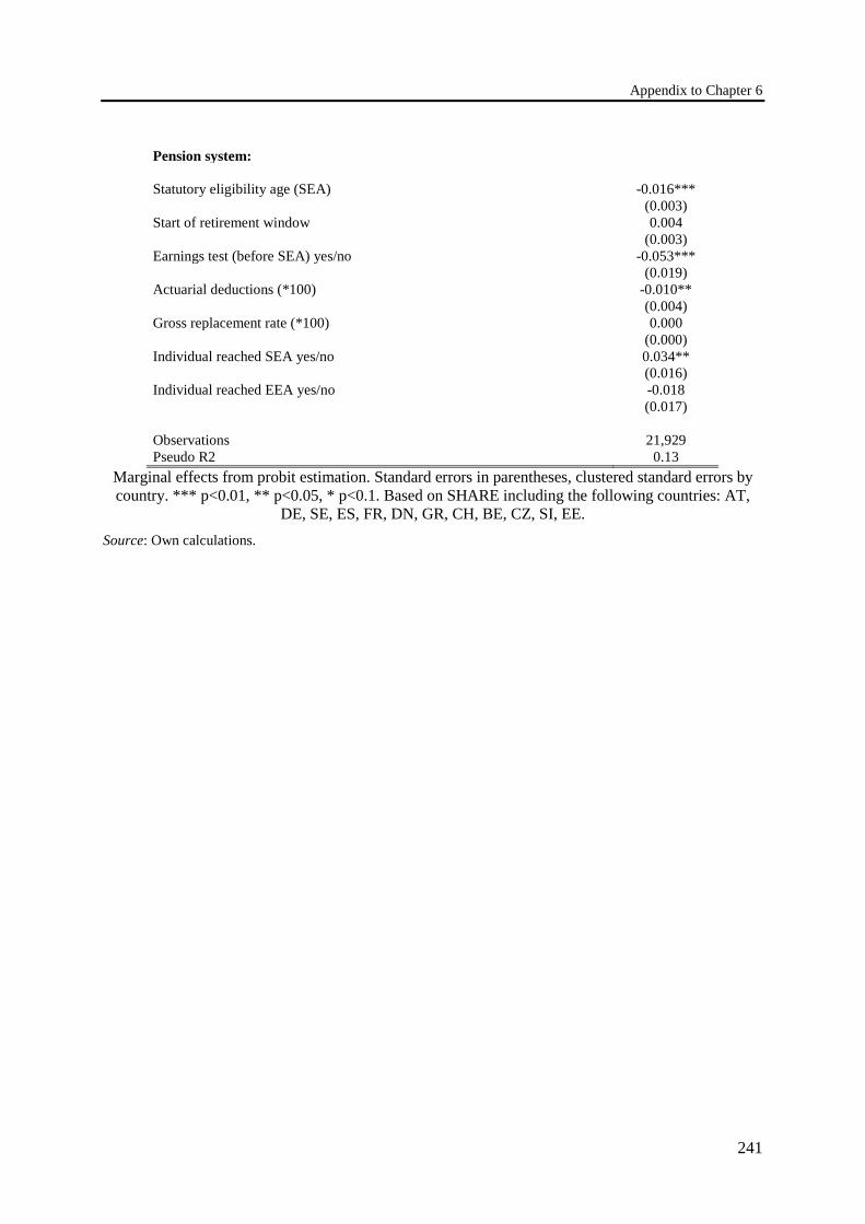
Appendix to Chapter 6
241
Pension system: Statutory eligibility age (SEA) -0.016*** (0.003) Start of retirement window 0.004 (0.003) Earnings test (before SEA) yes/no -0.053*** (0.019) Actuarial deductions (*100) -0.010** (0.004) Gross replacement rate (*100) 0.000 (0.000) Individual reached SEA yes/no 0.034** (0.016) Individual reached EEA yes/no -0.018 (0.017) Observations 21,929 Pseudo R2 0.13
Marginal effects from probit estimation. Standard errors in parentheses, clustered standard errors by country. *** p<0.01, ** p<0.05, * p<0.1. Based on SHARE including the following countries: AT,
DE, SE, ES, FR, DN, GR, CH, BE, CZ, SI, EE. Source: Own calculations.
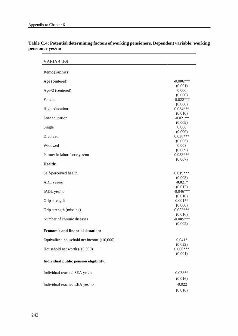
Appendix to Chapter 6
242
Table C.4: Potential determining factors of working pensioners. Dependent variable: working pensioner yes/no
VARIABLES Demographics: Age (centered) -0.006*** (0.001) Age^2 (centered) 0.000 (0.000) Female -0.022*** (0.008) High education 0.034*** (0.010) Low education -0.021** (0.009) Single 0.006 (0.009) Divorced 0.038*** (0.005) Widowed 0.008 (0.009) Partner in labor force yes/no 0.033*** (0.007) Health: Self-perceived health 0.019*** (0.003) ADL yes/no -0.021* (0.012) IADL yes/no -0.046*** (0.010) Grip strength 0.001** (0.000) Grip strength (missing) 0.052*** (0.016) Number of chronic diseases -0.005*** (0.002)
Economic and financial situation: Equivalized household net income (/10,000) 0.041* (0.022) Household net worth (/10,000) 0.006*** (0.001)
Individual public pension eligibility: Individual reached SEA yes/no 0.038** (0.016) Individual reached EEA yes/no -0.022 (0.016)
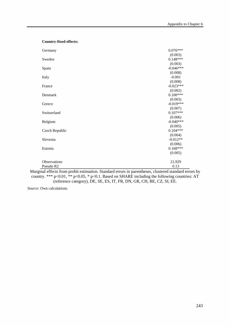
Appendix to Chapter 6
243
Country-fixed effects: Germany 0.076*** (0.003) Sweden 0.148*** (0.003) Spain -0.046*** (0.008) Italy -0.001 (0.008) France -0.023*** (0.002) Denmark 0.100*** (0.003) Greece -0.019*** (0.007) Switzerland 0.107*** (0.006) Belgium -0.040*** (0.005) Czech Republic 0.104*** (0.004) Slovenia -0.012** (0.006) Estonia 0.168*** (0.005) Observations 21,929 Pseudo R2 0.13
Marginal effects from probit estimation. Standard errors in parentheses, clustered standard errors by country. *** p<0.01, ** p<0.05, * p<0.1. Based on SHARE including the following countries: AT
(reference category), DE, SE, ES, IT, FR, DN, GR, CH, BE, CZ, SI, EE. Source: Own calculations.
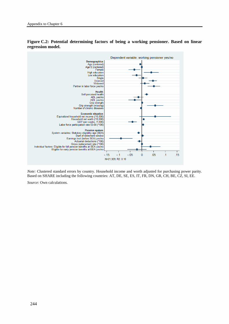
Appendix to Chapter 6
244
Figure C.2: Potential determining factors of being a working pensioner. Based on linear regression model.
Note: Clustered standard errors by country. Household income and worth adjusted for purchasing power parity. Based on SHARE including the following countries: AT, DE, SE, ES, IT, FR, DN, GR, CH, BE, CZ, SI, EE.
Source: Own calculations.

Appendix to Chapter 6
245
Table C.5: Potential determining factors of working pensioners. Dependent variable: working pensioner yes/no. Based on linear regression model.
VARIABLES Demographics: Age (centered) -0.006*** (0.001) Age^2 (centered) 0.000 (0.000) Female -0.032** (0.011) High education 0.040** (0.014) Low education -0.023** (0.009) Single 0.005 (0.009) Divorced 0.047*** (0.008) Widowed 0.013 (0.009) Partner in labor force yes/no 0.051*** (0.012)
Health: Self-perceived health 0.020*** (0.003) ADL yes/no -0.014 (0.010) IADL yes/no -0.030** (0.013) Grip strength 0.001** (0.000) Grip strength (missing) 0.057*** (0.016) Number of chronic diseases -0.004** (0.002)
Economic and financial situation: Equivalized household net income (/10,000) 0.057* (0.031) Household net worth (/10,000) 0.008*** (0.001) GDP (per-capita, /1,000) -0.040*** (0.008) Labor force participation rate 55–64 (*100) 0.005*** (0.001)
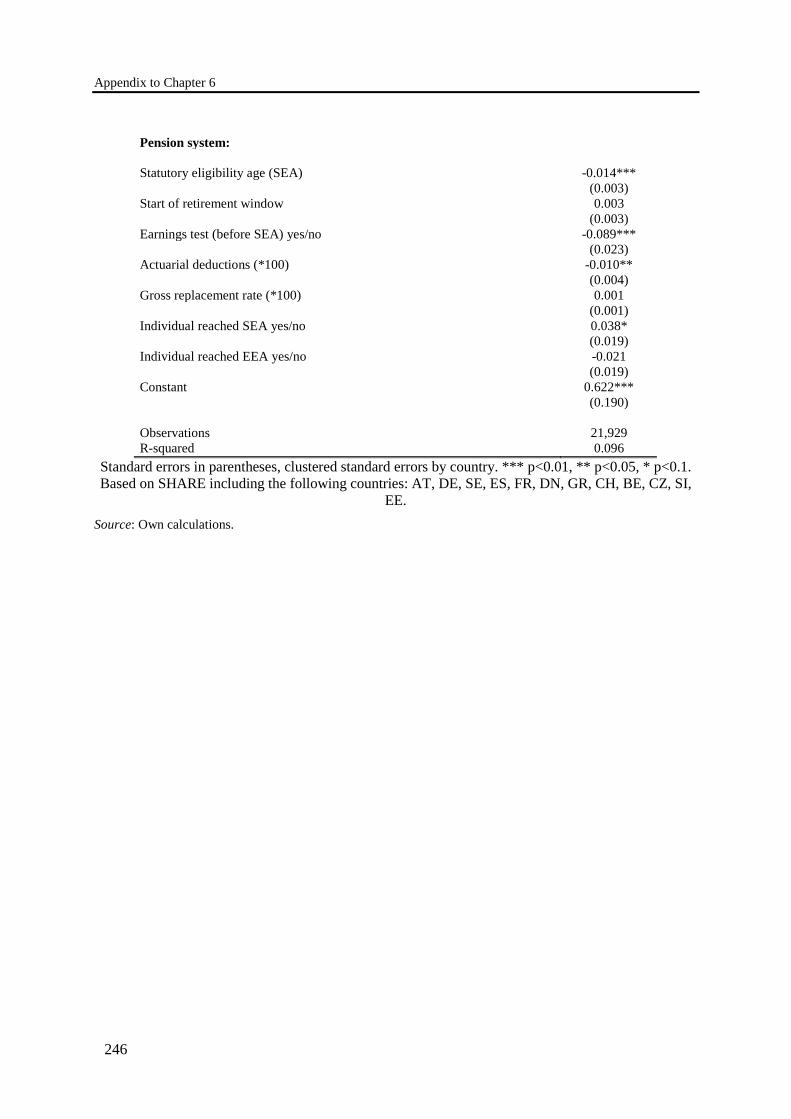
Appendix to Chapter 6
246
Pension system: Statutory eligibility age (SEA) -0.014*** (0.003) Start of retirement window 0.003 (0.003) Earnings test (before SEA) yes/no -0.089*** (0.023) Actuarial deductions (*100) -0.010** (0.004) Gross replacement rate (*100) 0.001 (0.001) Individual reached SEA yes/no 0.038* (0.019) Individual reached EEA yes/no -0.021 (0.019) Constant 0.622*** (0.190) Observations 21,929 R-squared 0.096
Standard errors in parentheses, clustered standard errors by country. *** p<0.01, ** p<0.05, * p<0.1. Based on SHARE including the following countries: AT, DE, SE, ES, FR, DN, GR, CH, BE, CZ, SI,
EE. Source: Own calculations.
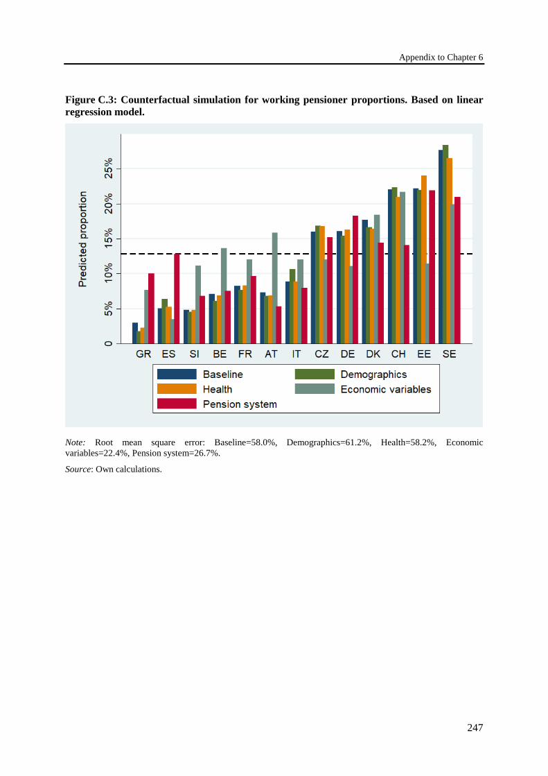
Appendix to Chapter 6
247
Figure C.3: Counterfactual simulation for working pensioner proportions. Based on linear regression model.
Note: Root mean square error: Baseline=58.0%, Demographics=61.2%, Health=58.2%, Economic variables=22.4%, Pension system=26.7%.
Source: Own calculations.

248
249
References
Abadie, A. and J. Gardeazabal (2003). ‘The economic costs of conflict: a case study of the Basque
Country’, The American Economic Review, 93 (1), 113-132.
Abadie, A., J. Diamond and J. Hainmueller (2010). ‘Synthetic control methods for comparative case
studies: estimating the effect of California’s tobacco control program’, Journal of the
American Statistical Association, 105 (490), 493-505.
Abadie, A., A. Diamond and J. Hainmueller (2015). ‘Comparative politics and the synthetic control
method’, American Journal of Political Science, 59 (2), 495-510.
Acemoglu, D., S. Johnson, A. Kermani, J. Kwak, and T. Mitton (2016). ‘The value of connections
in turbulent times: evidence from the United States’, Journal of Financial Economics, 121
(2), 368-391.
Albanese, A., B. Cockx and Y. Thuy (2015). ‘Working time reductions at the end of the career. Do
they prolong the time spent in employment?’, IZA Discussion Paper, 9619, IZA: Bonn.
Athey, S. and G. W. Imbens (2017). ‘The state of applied econometrics: causality and policy
evaluation’, Journal of Economic Perspectives, 31 (2), 3-32.
Australian Bureau of Statistics (2016). ‘2011 Census of Population and Housing: employment,
income and unpaid work’ TableBuilder [Online] Available at:
http://www.abs.gov.au/websitedbs/censushome.nsf/home/tablebuilder?opendocument&na
vpos=240 [Accessed 11 November 2016].
References
250
Australian Government (2004). ‘A more flexible and adaptable retirement income system’
[Online] Available at:
http://demographics.treasury.gov.au/content/_download/flexible_retirement_income_syste
m/flexible_retirement_income_system.pdf [Accessed 11 November 2016].
Australian Government (2015). ‘Superannuation policy for post-retirement’, Productivity
Commission Research Paper, 2, Supplementary Papers: Canberra.
Barr, N. and P. Diamond (2010). Pension Reform – A Short Guide, Oxford University Press:
Oxford.
Barro, R. and J.-W. Lee (2013). ‘A new data set of educational attainment in the world, 1950-2010’,
Journal of Development Economics, 104, 184-198.
Bilgel, F. and B. Galle (2015). ‘Financial incentives for kidney donation: a comparative case study
using synthetic controls’, Journal of Health Economics, 43, 103-117.
Billmeier, A. and T. Nannicini (2013). ‘Assessing economic liberalization episodes: a synthetic
control approach’, The Review of Economics and Statistics, 95 (3), 983-1001.
Bloemen, H., S. Hochguertel and J. Zweerink (2014). ‘Gradual retirement: a pathway with a
future?’, Netspar Panel Paper, 41, Netspar: Tilburg.
Bohn, S., M. Lofstrom and S. Raphael (2014). ‘Did the 2007 Legal Arizona Workers Act reduce
the state’s unauthorized immigrant population?’, The Review of Economics and Statistics,
96 (2), 258-269.
Börsch-Supan, A. (1992). ‘Population aging, social security design, and early retirement’, Journal
of Institutional and Theoretical Economics, 148, 533-557.
Börsch-Supan, A. (2005). ‘The 2005 pension reform in Finland’, Finnish Centre For Pensions,
Working Papers 2005:1. Rentenalter, Wünsche – Bedingungen – Möglichkeiten’,
Materialien zur Bevölkerungswissenschaft, 129, Bundesinstitut für
Bevölkerungsforschung: Wiesbaden.
Börsch-Supan, A. (2007). ‘Rational pension reform’, Geneva Papers on Risk and Insurance: Issues
and Practice, 4, 430-446.
References
251
Börsch-Supan, A., M. Brandt, C. Hunkler, T. Kneip, J. Korbmacher, F. Malter, B. Schaan, S. Stuck,
and S. Zuber (2013). ‘Data resource profile: the Survey of Health, Ageing and Retirement
in Europe (SHARE)’, International Journal of Epidemiology, 42 (4), 1-10.
Börsch-Supan, A., A. Brugiavini and E. Croda (2009). ‘The role of institutions and health in
European patterns of work and retirement’, Journal of European Social Policy, 19 (4), 341-
358.
Börsch-Supan, A., T. Bucher-Koenen, N. Goll, and V. Kutlu Koc (2018). ‘Dangerous flexibility –
retirement reforms reconsidered’, Economic Policy, 33 (4), 315-355.
Börsch-Supan, A., T. Bucher-Koenen and F. Hanemann (2020b). ‘Early Determinants of Work
Disability in an International Perspective’, Demography, forthcoming.
Börsch-Supan, A., T. Bucher-Koenen, S. Kluth, M. Haupt, and N. Goll (2015). ‘Vor- und Nachteile
höherer Flexibilität als Instrument zur Erhöhung der Beschäftigung Älterer’, MEA
Discussion Paper 06-2015: Munich.
Börsch-Supan, A., T. Bucher-Koenen, N. Goll, and F. Hanemann (2019a). ‘Targets missed: Three
case studies exploiting the linked SHARE-RV data’, MEA Discussion Paper 04-2019:
Munich.
Börsch-Supan, A. and C. Coile (2019). ‘Reforms and retirement incentives: introduction and
summary’, [Online] Available at: https://www.nber.org/chapters/c14190.pdf [Accessed
21 January 2020], preliminary draft for Börsch-Supan, A. and C. Coile (eds, forthcoming).
Social Security Programs and Retirement around the World: Reforms and Retirement
Incentives, NBER book series – International Social Security, forthcoming from University
of Chicago Press, preliminary drafts of single country chapters [Online] Available at:
https://www.nber.org/books/bors-1 [Accessed 14 January 2020].
Börsch-Supan, A. and I. Ferrari (2019). ‘Old-age labor force participation in Germany: What
explains the trend reversal among men and the steady increase among women?’, In:
Coile, C., K. Milligan and D. A. Wise (eds, 2019), Social Security Programs and Retirement
around the World: Working Longer. National Bureau of Economic Research, University of
Chicago Press: Chicago and London.
References
252
Börsch-Supan, A., I. Ferrari, N. Goll, and J. Rausch (2020). ‘Retirement Decisions in Germany:
Micro-Modelling’, mimeo, forthcoming In: Börsch-Supan, A. and C. Coile (eds,
forthcoming), NBER book series – International Social Security, forthcoming from
University of Chicago Press: Chicago and London.
Börsch-Supan, A., M. Gasche, M. Haupt, S. Kluth, and J. Rausch (2012). ‘Ökonomische Analyse
des Rentenreformpakets der Bundesregierung’, MEA Discussion Paper 05-2012: Munich.
Börsch-Supan A., K. Härtl and D. N. Leite (2016). ‘Social security and public insurance’, In:
Piggott, J. and A. Woodland (eds, 2016), Handbook of the Economics of Population Aging,
Vol. 1B, North Holland (Elsevier), Amsterdam, The Netherlands, 781-864.
Börsch-Supan, A. and H. Jürges (2012). ‘Disability, pension reform, and early retirement in
Germany’, In: Wise, D. A. (ed., 2012), Social Security Programs and Retirement around
the World. Historical Trends in Mortality and Health, Employment, and Disability
Insurance Participation and Reforms, 277-300, The University of Chicago Press: Chicago
and London.
Börsch-Supan, A. and C. Quinn (2015). ‘Taxing pensions and retirement benefits in Germany’,
MEA Discussion Paper 10-2015: Munich.
Börsch-Supan, A., J. Rausch and N. Goll (2019b). ‘Social security reforms and the changing
retirement behavior in Germany’, forthcoming In: Börsch-Supan, A. and C. Coile (eds,
forthcoming), preliminary draft [Online] Available at:
https://www.nber.org/chapters/c14195.pdf [Accessed 14 January 2020].
Börsch-Supan, A. and R. Schnabel (1998). ‘Social security and declining labor-force participation
in Germany’, The American Economic Review, 88 (2), 173-178.
Börsch-Supan, A. and R. Schnabel (1999). ‘Social security and retirement in Germany’, In: Gruber,
J. and D. A. Wise (eds, 1999), Social Security and Retirement around the World, 135-180,
University of Chicago Press: Chicago and London.
Bound, J. (1991). ‘Self-reported vs. objective measures of health in retirement models’, Journal of
Human Resources, 26, 106-138.
References
253
Brinch, C. N., O. L. Vestad and J. Zweimüller (2015). ‘Excess early retirement? Evidence from the
Norwegian 2011 pension reform’, University of Zurich Working Paper.
Brugiavini, A., R. E. Buia, G. Pasini, and G. Weber (2019a). ‘The Evolution of Incentives for
Retirement in Italy, 1980–2015’, forthcoming In: Börsch-Supan, A. and C. Coile (eds,
forthcoming), preliminary draft [Online] Available at:
https://www.nber.org/chapters/c14196.pdf [Accessed 19 January 2020].
Brugiavini, A., C. E. Orso, M. G. Genie, R. Naci, and G. Pasini (2019b). SHARE Job Episodes
Panel, Release version: 7.0.0. SHARE-ERIC.’ Data set. DOI: 10.6103/SHARE.jep.700.
Bucher-Koenen, T., I. Ferrari and Y. Pettinicchi (2019). ‘The role of pension knowledge in labour
supply decisions: evidence from Europe’, mimeo.
Büsch, V., J. Dorbritz, T. Heien, and F. Micheel (2010). ‘Weiterbeschäftigung im Rentenalter,
Wünsche – Bedingungen – Möglichkeiten’, Materialien zur Bevölkerungswissenschaft,
129, Bundesinstitut für Bevölkerungsforschung: Wiesbaden.
Card, D (1990). ‘The impact of the Mariel Boatlift on the Miami labor market’, Industrial and
Labor Relations Review, 43 (2), 245-57.
Caro, F., R. Morris and J. Norton (2000). Advancing Aging Policy as the 21st Century Begins,
Haworth Press: New York.
Cavallo, E., S. Galiani, I. Noy, and J. Pantano (2013). ‘Catastrophic natural disasters and economic
growth’, The Review of Economics and Statistics, 95 (5), 1549-1561.
Charni, K. and S. Bazen (2017). ‘Do earnings really decline for older workers?’, International
Journal of Manpower, 38 (1), 4-24.
Cihlar, V., A. Mergenthaler and F. Micheel (2014). ‘Erwerbsarbeit & informelle Tätigkeiten der
55- bis 70-Jährigen: transition and old age potential (TOP)’, Bundesministerium für
Bevölkerungsforschung: Wiesbaden [Online] Available at:
https://www.bib.bund.de/Publikation/2014/pdf/Erwerbstaetigkeit-und-informelle-
Taetigkeiten-der-55-bis-70-Jaehrigen-in-Deutschland.pdf?__blob=publicationFile&v=2
[Accessed 21 January 2020].
References
254
Coile, C. (2018). ‘The evolution of retirement incentives in the U.S.’, November, NBER Working
Paper 25281: Cambridge, Massachusetts.
Coile, C. and J. Gruber (2001). ‘Social security incentives for retirement’. In: Wise, D. A. (ed.,
2001), Themes in the Economics of Aging, 311-354. University of Chicago Press: Chicago
and London.
Coile, C., K. Milligan and D. A. Wise (eds, 2019). Social Security Programs and Retirement around
the World: Working Longer. National Bureau of Economic Research, University of Chicago
Press: Chicago and London.
Commission for Sustainability in Financing the Social Security Systems (Kommission für die
Nachhaltigkeit in der Finanzierung der Sozialen Sicherungssysteme) (2003). Nachhaltigkeit
in der Finanzierung der Sozialen Sicherungssysteme. Bericht der Kommission.
Bundesministerium für Gesundheit und Soziale Sicherheit, Berlin. [Online] Available at:
https://www.bmas.de/SharedDocs/Downloads/DE/PDF-Publikationen/c318-
nachhaltigkeit-in-der-finanzierung-der-sozialen-
sicherungssysteme.pdf?__blob=publicationFile [Accessed 24 January 2020].
Delsen, L. (1996). ‘Gradual retirement: lessons from the Nordic countries and the Netherlands’,
European Journal of Industrial Relations, 2 (1), 55-67.
Deutscher Bundestag (2014). ‘Gesetz über Leistungsverbesserungen in der gesetzlichen
Rentenversicherung (RV-Leistungsverbesserungsgesetz)’, Bundesdrucksache 18/909:
Berlin.
Deutscher Bundestag (2020). ‘Bundestag beschließt die Einführung der Grundrente’, [Online]
Available at: https://www.bundestag.de/dokumente/textarchiv/2020/kw27-de-grundrente-
703572 [Accessed 6 July 2020].
Deutsche Rentenversicherung Bund (DRV) (2011). ‘FDZ-Biografiedatensatz für die
Biografiedaten der Versicherten’ (VSKT).
Deutsche Rentenversicherung Bund (DRV) (2017). ‘Rentenversicherung in Zeitreihen’, DRV-
Schriften, Band 22: Berlin.
References
255
Deutsche Rentenversicherung Bund (DRV) (2020). ‘Chronik’ [Online] Available at:
http://forschung.deutsche-rentenversicherung.de/ForschPortalWeb/ressource?key=chronik
[Accessed 3 July 2020].
Deutsche Rentenversicherung Bund (DRV) (2018). ‘Rentenversicherung in Zahlen 2018’ [Online]
Available at: https://www.deutsche-
rentenversicherung.de/cae/servlet/contentblob/238692/publicationFile/61815/01_rv_in_za
hlen_2013.pdf [Accessed 14 January 2018].
Deutsche Rentenversicherung Bund (DRV) (2019). ‘Statistikportal der Rentenversicherung’
[Online] Available at: https://statistik-rente.de/drv/ [Accessed 4 February 2019].
Devisscher, S. and D. Sanders (2008). ‘Ageing and life-course issues: the case of the career break
scheme (Belgium) and the life-course regulation (Netherlands)’, In: OECD, Modernising
Social Policy for the New Life Course, OECD Publishing: Paris [Online] Available at:
http://dx.doi.org/10.1787/9789264041271-5-en [Accessed 13 October 2015].
Dingemans, E., K. Henkens and H. van Solinge (2017). ‘Working retirees in Europe: individual and
societal determinants’, Work, Employment and Society, 31 (6), 972-991.
Dingemans, E. and K. Henkens (2019). ‘Working after retirement and life satisfaction: cross-
national comparative research in Europe’, Research on Aging, 41 (7), 648-669.
Dingemans, E. and K. Möhring (2019). ‘A life course perspective on working after retirement: What
role does the work history play?’, Advances in Life Course Research, 39, 23-33.
Disney, R. and S. Smith (2002). ‘The labour supply effect of the abolition of the earnings rule for
older workers in the United Kingdom’, The Economic Journal, 112 (478), C136-C152.
Dolls, M. and C. Krolage (2019). ‘The Effects of Early Retirement Incentives on Retirement
Decisions’, ifo Working Paper, No. 291, ifo Institute: Munich.
References
256
Dorbritz, J. and F. Micheel (2010). ‘Weiterbeschäftigung im Rentenalter – Potentiale, Einstellungen
und Bedingungen’, Bevölkerungsforschung Aktuell, 31 (3), 2-7.
Driscoll, J. and A. Kraay (1998). ‘Consistent covariance matrix estimation with spatially dependent
panel data’, The Review of Economics and Statistics, 80 (4), 549-560.
Duval, R. (2003). ‘The retirement effects of old-age pension and early retirement schemes in OECD
countries’, OECD Economics Department Working Papers, 370, OECD Publishing: Paris.
Engels, B., J. Geyer and P. Haan (2017). ‘Pension Incentives and early retirement’, Labour
Economics 47, 216-231.
Ellguth, P. and B. Koller (2000). ‘Frühverrentung: Arbeitsmarktentlastung durch Altersteilzeit’,
IAB Materials, 1, 4-5.
Eurofound (2012). Income from Work after Retirement in the EU, Publications Office of the
European Union: Luxembourg.
Eurofound (2016). Extending Working Lives through Flexible Retirement Schemes: Partial
Retirement, Publications Office of the European Union: Luxembourg.
European Commission (1995). ‘Developments in employment policies in Europe’ Series produced
from the MISEP network.’ Employment Observatory, 49, Spring 1995 [Online] Available
at: http://aei.pitt.edu/43858/1/A6317.pdf [Accessed 9 March 2017].
European Commission (2011). Age and Employment, European Commission Justice: Brussels.
Ferman, B., C. Pinto and V. Possebom (2020). ‘Cherry picking with synthetic controls’, Journal of
Policy Analysis and Management, accepted and forthcoming.
Finnish Centre for Pensions (2014). ‘Goals to extend working life will be concretized in pensions
in 2017’, [Online] Available at: https://www.etk.fi/en/the-pension-system/dynamic-
pension-scheme/pension-reform-in-2017/ [Accessed 13 March 2017].
Freire, D. (2018). ‘Evaluating the effect of homicide prevention strategies in São Paulo, Brazil: a
synthetic control approach’, Latin American Research Review, 53 (2), 231-249.
References
257
Gale, C. R., C. N. Martyn, C. Cooper, and A. A. Sayer (2007). ‘Grip strength, body composition,
and mortality’, International Journal of Epidemiology, 36 (1), 228-235.
Galiani, S. and B. Quistorff (2016). ‘The synth_runner package: utilities automate synthetic control
estimation using synth’, University of Maryland Working Paper, [Online] Available at:
http://econweb.umd.edu/~galiani/files/synth_runner.pdf [Accessed 11 November 2016].
Gasche, M. (2012). ‘Was sind die richtigen Rentenabschläge? – Neue Perspektiven’, Jahrbuch für
Wirtschaftswissenschaften, 63 (2), 187-235.
Gasche, M. and C. Krolage (2012). ‘Gleitender Übergang in die Rente durch Flexibilisierung der
Teilrente’, Sozialer Fortschritt, 61 (7), 149-159.
Geyer, J., P. Haan, A. Hammerschmid, and M. Peters (2020). ‘Labor Market and Distributional
Effects of an Increase in the Retirement Age’, Labour Economics 65, Article 101817.
Geyer, J. and C. Welteke (2019). ‘Closing routes to retirement for women: how do they respond?’,
Journal of Human Resources (forthcoming), [Online] Available at:
DOI:10.3368/jhr.56.1.0717-8947R2 [Accessed 29 June 2020].
Gielen, A. C. (2009). ‘Working hours flexibility and older workers’ labor supply’, Oxford
Economic Papers, 61, 240-274.
Giesecke, M. (2018). ‘The Effect of Benefit Reductions on the Retirement Age: The Heterogeneous
Response of Manual and Non-Manual Workers’, Review of Income and Wealth, 64 (1), 213-
238.
Gobillon, L. and T. Magnac (2016). ‘Regional policy evaluation: interactive fixed effects and
synthetic controls’, The Review of Economics and Statistics, 98 (3), 535-551.
Goebel, J., M. M. Grabka, S. Liebig, M. Kroh, D. Richter, C. Schröder, and J. Schupp (2019). ‘The
German Socio-Economic Panel Study (SOEP)’, Jahrbücher für Nationalökonomie und
Statistik/Journal of Economics and Statistics, 239 (2), 345-360.
Graf, N., H. Hofer, R. Sellner, R. Winter-Ebmer, and A. Wroblewskiet (2008). Evaluierung der
arbeitsmarktpolitischen Wirkungen des Altersteilzeitgeldes: Anreizstrukturen, Wirkungen
und Implikationen, Studie im Auftrag des Bundesministeriums für Wirtschaft und Arbeit
(BMWA), Institute for Advanced Studies: Vienna.
References
258
Graf, N., H. Hofer and R. Winter-Ebmer (2011). ‘Labour supply effects of a subsidized old-age
part-time scheme in Austria’, Zeitschrift für ArbeitsmarktForschung, 44, 217-229.
Gruber, J. and D. A. Wise (eds, 1999). Social Security Programs and Retirement around the World,
University of Chicago Press: Chicago.
Gruber, J. and D. A. Wise (eds, 2004). Social Security Programs and Retirement around the World:
Micro-Estimation. University of Chicago Press: Chicago.
Gruber, J. and D. A. Wise (eds, 2010). Social Security Programs and Retirement around the World:
The Relationship to Youth Employment, University of Chicago Press: Chicago.
Gustman, A. L. and T. L. Steinmeier (1983). ‘Minimum hours constraints and retirement behavior’,
Contemporary Policy Issues, a supplement to Economic Inquiry, 1 (3), 77-91.
Gustman, A. L. and T. L. Steinmeier (1984). ‘Partial retirement and the analysis of retirement
behavior’, ILR Review, 37 (3), 403-415.
Gustman, A. L. and T. L. Steinmeier (1986). ‘A structural retirement model’, Econometrica, 54 (3),
555-584.
Gustman, A. L. and T. L. Steinmeier (2004). ‘Minimum hours constraints, job requirements and
retirement’, October, NBER Working Paper 10876: Cambridge, Massachusetts.
Hahn, J. and R. Shi (2017). ‘Synthetic control and inference’, Econometrics, 5 (4), 52.
Hanel, B. (2010). ‘Financial incentives to postpone retirement and further effects on employment –
evidence from a natural experiment’, Labour Economics, 17 (3), 474-486.
Hanel, B. (2012). ‘The Effect of Disability Pension Incentives on Early Retirement Decisions’.
Labour Economics, 19 (4), 595-607.
Hanel, B. and Riphahn, R. T. (2012). ‘The timing of retirement – New evidence from Swiss female
workers’. Labour Economics, 19 (5), 718-728.
Hansen, H. (2001). ‘Active strategies for older workers’, Working Paper 02:2001, The Danish
National Institute of Social Research: Copenhagen.
References
259
Hinrichs, P. (2012). ‘The effects of affirmative action bans on college enrollment, educational
attainment, and the demographic composition of universities’, The Review of Economics
and Statistics, 94 (3), 712-722.
Hoechle, D. (2007). ‘Robust standard errors for panel regressions with cross-sectional dependence’,
The Stata Journal, 7 (3), 281-312.
Holthausen, A., J. Rausch and C. B. Wilke (2012). ‘MEA-PENSIM 2.0: Weiterentwicklung eines
Rentensimulationsmodells, Konzeption und ausgewählte Anwendungen’, MEA Discussion
Paper 03-2012: Munich.
Huber, M., M. Lechner and C. Wunsch (2013). ‘The effect of firms’ partial retirement policies on
the labour market outcomes of their employees’, CESifo Working Paper, 4343: Munich.
Hurd, M. D. (1990). ‘Research on the elderly: economic status, retirement, and consumption and
saving’, Journal of Economic Literature, 28 (2), 565-637.
Hurd, M. D. (1996). ‘The effect of labor market rigidities on the labor force behavior of older
workers’, In: Wise, D. A. (ed., 1996), Advances in the Economics of Aging, 11-58,
University of Chicago Press: Chicago.
Hutchens, R. (2010). Worker characteristics, job characteristics, and opportunities for phased
retirement, Labour Economics, 17 (6), 1010-1021.
Hutchens, R. and K. Grace-Martin (2006). ‘Employer Willingness to Permit Phased Retirement:
Why Are Some More Willing than Others?’, Industrial and Labor Relations Review, 59 (4),
525-546.
Idler, E. L. and Y. Benyamini (1997). ‘Self-rated health and mortality: a review of twenty-seven
community studies’, Journal of Health and Social Behavior, 38 (1), 21-37.
Ilmakunnas, P. and S. Ilmakunnas (2006). ‘Gradual retirement and lengthening of working life’,
HECER Discussion Paper, 121: Helsinki.
Jylhä, M. (2009). ‘What is self-rated health and why does it predict mortality? Towards a unified
conceptual model’, Social Science & Medicine, 69 (3), 307-316.
References
260
Kaul, A., S. Klößner, G. Pfeifer, and M. Schieler (2015). ‘Synthetic control methods: Never use all
pre-intervention outcomes as economic predictors’ [Online] Available at:
http://www.oekonometrie.uni-saarland.de/papers/SCM_Predictors.pdf [Accessed
11 November 2016].
Kaul, A., S. Klößner, G. Pfeifer, and M. Schieler (2018). ‘Synthetic control methods: Never use all
pre-intervention outcomes together with covariates’ [Online] Available at:
http://www.oekonometrie.uni-saarland.de/papers/SCM_Predictors.pdf [Accessed
6 November 2019].
Kleven, H. J., C. Landais and E. Saez (2013). ‘Taxation and international migration of superstars:
evidence from the European football market’, The American Economic Review, 103 (5),
1892-1924.
Kreif, N., R. Grieve, D. Hangartner, A. J. Turner, S. Nikolova, and M. Sutton (2016). ‘Examination
of the synthetic control method for evaluating health policies with multiple treated units’,
Health Economics, 25, 1514-1528.
Kremalis (2018). ‘International age discrimination. Greece. October 11, 2018’ [Online] Available
at: http://www.agediscrimination.info/international-age-discrimination/greece [Accessed
4 November 2019].
Lindecke, C., D. Voss-Dahm and S. Lehndorff (2007). ‘Altersteilzeit, Erfahrungen und
Diskussionen in Deutschland und anderen EU-Ländern’, Arbeitspapier 142, Hans-Böckler-
Stiftung: Düsseldorf.
Liu, S. (2015). ‘Spillovers from universities: evidence from the land-grant program’, Journal of
Urban Economics, 87, 25-41.
Lynch, J. and M. Myrskyl (2009). ‘Always the third rail? Pension income and policy preferences in
European democracies’, Comparative Political Studies, 42, 1068-1097.
References
261
MISSOC (2013). ‘Comparative Tables on Social Protection’ (Austria, Germany, Sweden, Spain,
Italy, France, Denmark, Greece, Switzerland, Belgium, Czech Republic, Poland,
Luxembourg, Portugal, Slovenia, Estonia, Croatia), from European Commission
Employment, Social Affairs, and Equal opportunities [Online] Available at:
https://www.missoc.org/missoc-database/comparative-tables/ [Accessed 20 March 2019].
Myck, M. (2010). “Wages and ageing: Is there evidence for the ‘Inverse-U’ profile?’, Oxford
Bulletin of Economics and Statistics, 72 (3), 282-306.
Naisbitt, J. (1982). Megatrends: Ten New Directions Transforming Our Lives, Warner Books, Inc.
Naisbitt, J. and P. Aburdene (1990). Megatrends 2000: Ten New Directions for the 1990s, Avon
Books, US.
Nannicini, T. and A. Billmeier (2011). ‘Economies in transition: How important is trade openness
for growth?’, Oxford Bulletin of Economics and Statistics, 73 (3), 287-314.
National Insurance Institute of Israel (2019). ‘Old Age’, [Online] Available at:
https://www.btl.gov.il/English%20Homepage/Benefits/Old%20Age%20Insurance/Pages/d
efault.aspx [Accessed 10 December 2019].
O’Neill, S., N. Kreif, R. Grieve, M. Sutton, and J. S. Sekhon (2016). ‘Estimating causal effects:
considering three alternatives to difference-indifferences estimation’, Health Services and
Outcomes Research Methodology, 16, 1-21.
OECD (2005a). Ageing and Employment Policies: France 2005, OECD Publishing: Paris.
OECD (2005b). Pensions at a Glance 2005, OECD Publishing: Paris.
OECD (2011a). Pensions at a Glance 2011, OECD Publishing: Paris.
OECD (2011b). ‘Linking pensions to life expectancy’, In Pensions at a Glance 2011: Retirement-
income Systems in OECD and G20 Countries, OECD Publishing: Paris [Online] Available
at: http://dx.doi.org/ 10.1787/pension_glance-2011-9-en [Accessed 13 March 2017].

References
262
OECD (2013a). ‘Directorate for Employment, Labour and Social Affairs, Pension system, Ageing
and Employment Policies – Statistics on average effective age of retirement, Average
effective age of retirement versus the official age in 2012 in OECD countries’ [Online]
Available at: http://www.oecd.org/els/emp/Summary_2012_values.xls [Accessed
5 November 2015].
OECD (2013b). Pensions at a Glance 2013, OECD: Paris.
OECD (2013c). ‘Country profiles’, In: Pensions at a Glance 2013, OECD Publishing: Paris.
OECD (2013d). ‘GDP per head, US $, constant prices, constant PPPs, reference year 2010’,
OECD.Stat, Data, National Accounts, Annual National Accounts, Main Aggregates, Gross
Domestic Product (GDP).
OECD (2013e). ‘Labor force participation rate’, OECD.Stat, Data, Labor, Labor Force Statistics,
LFS by sex and age – indicators.
OECD (2014a). Ageing and Employment Policies: France 2014: Working Better with Age,
Assessment and main recommendations, OECD Publishing: Paris.
OECD (2014b). ‘Gross and net pension replacement rates. Pension entitlements as percentage of
pre-retirement earning, single persons’, OECD Pension Statistics.
OECD (2015a). Ageing and Employment Policies: Poland 2015, OECD Publishing: Paris.
OECD (2015b). Pensions at a Glance 2015, OECD: Paris.
OECD (2015c). Ageing and Employment Policies: Denmark 2015, Working Better with Age,
Assessment and Main Recommendations, OECD Publishing: Paris.
OECD (2016a). ‘Level of GDP per capita and productivity’, OECD.Stat, Data, Economy,
Productivity, GDP per capita and productivity levels.
OECD (2016b). ‘Life expectancy at birth’, OECD.Stat, Data, Health Status, Life expectancy.
OECD (2017). Pensions at a Glance 2017, OECD Publishing: Paris.
References
263
OECD (2018a). ‘LFS by sex and age – indicators’ [Online] Available at:
http://stats.oecd.org/Index.aspx?DataSetCode=LFS_SEXAGE_I_R [Accessed 14 January
2020].
OECD (2018b). ‘Table I.5. Average personal income tax and social security contribution rates on
gross labour income’ [Online] Available at:
http://stats.oecd.org/Index.aspx?DataSetCode=TABLE_I5 [Accessed 14 January 2020].
Palmer, E. (2000). ‘The Swedish pension reform model: framework and issues’, Social Protection
Discussion Paper, 0012, The World Bank: Washington, D.C.
Piggott, J. and A. Woodland (eds, 2016). ‘Handbook of the Economics of Population Aging’,
Elsevier: North Holland.
Queisser, M. and E. Whitehouse (2006). ‘Neutral or fair? Actuarial concepts and pension-system
design’, OECD Social, Employment and Migration Working Papers, 40, OECD: Paris.
Reday-Mulvey, G. (2000). ‘Gradual retirement in Europe’, In: Caro, F., R. Morris and J. Norton
(eds, 2000), Advancing Aging Policy as the 21st Century Begins, 49-59, Haworth Press:
New York.
Riphahn, R. T. and R. Schrader (2019). ‘Institutional reforms and an incredible rise in old-age
employment’, Industrial and Labor Relations Review (forthcoming), [Online] Available at:
https://doi.org/10.1177/0019793919863378 [Accessed 19 July 2020].
Safire W. (2007). ‘The third rail’, The New York Times Magazine: New York.
Saia, A. (2017). ‘Choosing the open sea: the cost to the UK of staying out of the euro’, Journal of
International Economics, 108, 82-98.
Sen, A. (2002). ‘Health perception versus observation’, British Medical Journal, 324, 860-861.
Seibold, A. (2019). ‘Reference Points for Retirement Behavior: Evidence from German Pension
Discontinuities’, CESifo Working Paper No. 7799, CESifo: Munich.
Siddiqui, S. (1997). The pension incentive to retire: empirical evidence for West Germany,
Population Economics, 10, 463-486.
References
264
Social Security Administration (1985-2014). Social Security Programs throughout the World, SSA:
Washington, D. C., Geneva.
Social Policy and Law Shared Database (SPLASH database) (2012). Policy: Act Establishing
Measures for the Social Security System (40/2007), Information provided by Albert Sabater
[Online] Available at: https://splash-db.eu [Accessed 24 October 2019].
Social Policy and Law Shared Database (SPLASH database) (2019). ‘Data. Work&Retirement’
[Online] Available at: https://splash-db.eu/ [Accessed 10 October 2019].
Statens Offentliga Utredningar (2013). ‘Åtgärder för ett längre arbetsliv’, Slutbetänkande av
Pensionsåldersutredningen, 25.
Statistisches Bundesamt (2015). ‘Generationensterbetafeln für Deutschland, Modellrechnungen für
die Geburtsjahrgänge 1896-2009’. Statistisches Bundesamt: Wiesbaden.
Statistisches Bundesamt (2016). Mikrozensus, Bevölkerung und Erwerbstätigkeit. Stand und
Entwicklung der Erwerbstätigkeit in Deutschland. Statistisches Bundesamt: Wiesbaden.
Stearns, J. (2015). ‘The effects of paid maternity leave: evidence from temporary disability
insurance’, Journal of Health Economics, 43, 85-102.
Wanger, S. (2010). ‘Die Altersteilzeit im Zusammenspiel individueller und betrieblicher
Einflussfaktoren’, WSI Notifications, 63 (8), 395-403.
Warren, D. (2008). ‘Australia’s retirement income system: historical development and effects of
recent reforms’, Melbourne Institute Working Paper Series, 23: Melbourne.
Werding, M. (2007). ‘Versicherungsmathematisch korrekte Rentenabschläge für die gesetzliche
Rentenversicherung’, ifo Schnelldienst, 60 (16), 19-32.
Werding, M. (2012). ‘Rentenbemessung und Renteneintrittsalter: Korrekte Abschläge bei
vorzeitigem Rentenzugang’, mimeo, Lehrstuhl für Sozialpolitik und öffentliche Finanzen,
Ruhr-Universität Bochum: Bochum.
Wise, D. A. (ed., 1996). Advances in the Economics of Aging, University of Chicago Press:
Chicago.

References
265
Ye, H. (2018). ‘The effect of pension subsidies on retirement timing of older women: evidence from
a regression kink design’, IZA Discussion Paper, No. 11831, IZA - Institute of Labor
Economics: Bonn.

266

267

268