Embed Size (px)
Citation preview
Torque Vectoring
Linear Parameter-Varying Control for an Electric Vehicle
Vom Promotionsausschuss derTechnischen Universität Hamburg-Harburg
zur Erlangung des akademischen Grades
Doktor-Ingenieur (Dr.-Ing)
genehmigte Dissertation
vonGerd Kaiser
ausHeidelberg
2015
Gutachter:
Prof. Dr. Herbert Werner
Prof. Dr. Valentin Ivanov
Tag der mündlichen Prüfung:1. Dezember 2014
URN: urn:nbn:de:gbv:830-88212424
Acknowledgments
This external PhD thesis was carried out between December 2009 and December 2014 asco-operation between Intedis GmbH & Co. KG and Hamburg University of Technology(TUHH). The aim of this work is to improve vehicle dynamics for electric vehicles withtwo electric motors, using linear parameter-varying control.
My thanks to Professor Dr. Werner for his supervision of my thesis and his helpfuladvises on control science. Also, I want to thank him for giving me the chance to startmy PhD-thesis in the first place. In addition, I want to thank Professor Dr. ValentinIvanov from the Technische Universität Ilmenau for being my second assessor and illu-minating further questions on vehicle dynamics. And, I want to thank Professor Dr.-Ing.Weltin for being the chairperson of my examination. Additionally, I want to thank allPhD-students from the control science department for all enlightening discussions atTUHH.
I would like to thank Dr. Holzmann for his extensive support and advice during mywork at Intedis. Additionally, I want to thank all colleagues from the eFuture project;especially Fabian, Matthias, and Volker because the eFuture prototype would not berunning without your efforts. Also, I want to thank all colleagues and students whosupported this work at Intedis.
Finally, I want to thank my parents, family and friends for all their support and theirbelief in me.


I dedicate this thesis to my familyand to dear ones who did not see this day.

Summary
In this thesis, advanced control theory is applied to the problem of controlling an electricvehicle with independent propulsion actuators. Here, a linear parameter-varying (LPV)vehicle dynamics controller is designed and implemented to control two independentelectric machines driving the front wheels of a prototype vehicle developed as part of theEuropean project eFuture. The control concept is implemented on a standard automo-tive microcontroller and deals with safety, performance and efficiency limitations of thevehicle. The thesis is divided into three main parts:
• The first part deals with the vehicle dynamics and the torque vectoring application.To begin, the dynamics of the vehicle are analysed in Chapter 2, and severalvehicle models and tyre models are presented. The vehicle drivetrain is brieflydiscussed, and limitations and constraints on vehicle movement are pointed out.The validation of simulation models with experimental data is also shown. InChapter 3, several torque vectoring applications are analysed.
• The second part is concerned with control theory and controller design for torquevectoring. Chapter 4 reviews the modelling and control of LPV systems. Differentapproaches to LPV control are compared, and it is shown how non-linear vehicledynamics can be represented as LPV models. Chapter 5 investigates the influ-ence of actuator limitations on vehicle behaviour and explains how an anti-windupdesign is implemented to deal with saturations of the electric drivetrain. Thisanti-windup concept is extended to cope with spinning or locking wheels.
• The third part of the thesis presents the implementation of the control design andexperimental results using the prototype vehicle of the eFuture project. Chap-ter 6 discusses the general driveline software of the eFuture prototype and theinteraction of different software functions with torque vectoring. A discrete-timecontroller design is proposed and the fixed-point representation of the controlleris discussed. Chapter 7 discusses real test drives, which demonstrate the perfor-mance improvements achieved with torque vectoring, as compared to an equaltorque distribution, as typically used in conventional vehicles.
vii

Abstract
In this thesis, a torque vectoring control strategy is proposed for the propulsion ofan electric vehicle with two independent electric machines at the front wheels. Theproposed control scheme comprises a linear parameter-varying (LPV) controller and amotor torque and wheel slip limiter which deals with drivetrain saturations and wheel sliplimitations. This control strategy was implemented on a microcontroller in a test car. Aspart of the European project eFuture, test drives were carried out and measurements wereperformed in several test manoeuvres, which demonstrate the benefits of the proposedmethod as compared with equal torque distribution.
Key words: LPV systems, Torque vectoring, active yaw control, H∞ control, eFuture,single track model, vehicle dynamics, tyre model, anti-windup, chassis control, drive-train, fixed-point representation
KurzzusammenfassungZiel der Arbeit war die Entwicklung einer Antriebsmomenten-Verteilungsstrategie fürein elektrisches Fahrzeug. Ein Prototyp wird mit zwei elektrischen Maschinen an derVorderachse angetrieben. Die Antriebsmomenten-Verteilung besteht aus einem linearen,parameterveränderlichen (LPV) Fahrdynamik-Regler und einem Motormoment- undRadschlupf-Begrenzer. Das Regelkonzept wurde auf einem Mikrocontroller integriert,welcher für den automobilen Einsatz qualifiziert ist. Im Rahmen des europäischen Pro-jekts eFuture wurden mehrere Testfahrten durchgeführt, die die Vorteile der vorgeschla-genen Regelstrategie gegenüber einer Gleichverteilung des Antriebsmoments zeigen.
Schlüsselwörter: LPV-Systeme, LMI, Torque vectoring, aktive Gierraten-Regelung,H∞-Regelung, eFuture, Einspurmodell, Fahrdynamik, Reifenmodell, Anti-Windup, Fahr-werkregelung, Antriebsstrang, Festkomma-Arithmetik
ix

List of Publications
1. Concept of Through the Road Hybrid Vehicle (B. Chretien, F. Holzmann, G. Kaiser,S. Glaser, S. Mammar),In Proceedings of the Advanced Vehicle Control Conference(AVEC), Lough-borough, England, August 2010.
2. Torque Vectoring with a feedback and feed forward controller - applied to a throughthe road hybrid electric vehicle (G. Kaiser, F. Holzmann, B. Chretien, M. Korteand H. Werner),In Proceedings of the 2011 IEEE Intelligent Vehicles Symposium(IV), Baden-Baden, Germany, June, 2011.
3. Two-Degree-of-Freedom LPV Control for a through-the-Road Hybrid Electric Vehi-cle via Torque Vectoring (Q. Liu, G. Kaiser, S. Boonto, H. Werner, F. Holzmann,B. Chretien and M. Korte),In Proceedings of the 50th IEEE Conference on Decision and Control andEuropean Control Conference (CDC-ECC), Orlando, FL, USA, December2011.
4. Design of a robust plausibility check for an adaptive vehicle observer in an electricvehicle (M. Korte, G. Kaiser, V. Scheuch, F. Holzmann, H. Roth)In Proceedings of the 16th Advanced Microsystems for Automotive Appli-cations(AMAA), Berlin, Germany, May 2012.
5. A New Functional Architecture for the Improvement of eCar Efficiency and Safety(V. Scheuch, G. Kaiser, R. Straschill, F. Holzmann),In Proceedings of the 21st Aachener Colloquium Automobile and EngineTechnology, Aachen, Germany, October 2012.
6. Torque Vectoring for an Electric Vehicle - Using an LPV Drive Controller anda Torque and Slip Limiter (G. Kaiser, Q. Liu, C. Hoffmann, M. Korte and H.Werner),In Proceedings of the 51st IEEE Conference on Decision and Control(CDC),Maui, Hawaii, USA, December 2012.
7. LPV Torque Vectoring for an Electric Vehicle Using Parameter-Dependent Lya-punov Functions (M. Bartels, Q. Liu, G. Kaiser and H. Werner),In Proceedings of the 2013 American Control Conference(ACC), Washington,D.C., USA, June 2013.
xi
xii List of Publications
8. Robust Vehicle Observer to Enhance Torque Vectoring in an EV (M. Korte, F.Holzmann, G. Kaiser, H. Roth,),In Proceedings of the 5th Fachtagung: Steuerung und Regelung von Fahrzeu-gen und Motoren(AUTOREG), Baden-Baden, Germany, November 2013.
9. LPV Torque Vectoring for an Electric Vehicle with Experimental Validation (G.Kaiser, M. Korte, Q. Liu, C. Hoffmann and H. Werner),In Proceedings of the 19th World Congress of the International Federationof Automatic Control(IFAC), Cape Town, South Africa, August 2014.
Contents
Summary vii
Abstract ix
List of Publications xi
1 Introduction 11.1 Problem Description . . . . . . . . . . . . . . . . . . . . . . . . . . . . . . 21.2 Scope of Work . . . . . . . . . . . . . . . . . . . . . . . . . . . . . . . . . 41.3 Main Objective . . . . . . . . . . . . . . . . . . . . . . . . . . . . . . . . . 41.4 Scientific Contribution . . . . . . . . . . . . . . . . . . . . . . . . . . . . . 41.5 Thesis Overview . . . . . . . . . . . . . . . . . . . . . . . . . . . . . . . . 5
2 Automotive Vehicles 72.1 Vehicle Model . . . . . . . . . . . . . . . . . . . . . . . . . . . . . . . . . . 7
2.1.1 Global vehicle model . . . . . . . . . . . . . . . . . . . . . . . . . . 72.1.2 Dual-track model . . . . . . . . . . . . . . . . . . . . . . . . . . . . 102.1.3 Single-track model . . . . . . . . . . . . . . . . . . . . . . . . . . . 11
2.2 Vehicle Components . . . . . . . . . . . . . . . . . . . . . . . . . . . . . . 132.2.1 Wheels . . . . . . . . . . . . . . . . . . . . . . . . . . . . . . . . . 132.2.2 Propulsion system . . . . . . . . . . . . . . . . . . . . . . . . . . . 17
2.3 Model Calibration . . . . . . . . . . . . . . . . . . . . . . . . . . . . . . . 192.3.1 General driving . . . . . . . . . . . . . . . . . . . . . . . . . . . . . 202.3.2 Extreme driving manoeuvre . . . . . . . . . . . . . . . . . . . . . . 222.3.3 Motor torque . . . . . . . . . . . . . . . . . . . . . . . . . . . . . . 23
2.4 Automotive Vehicle: Conclusion . . . . . . . . . . . . . . . . . . . . . . . . 26
3 Torque Vectoring 273.1 History . . . . . . . . . . . . . . . . . . . . . . . . . . . . . . . . . . . . . 27
3.1.1 Active safety functions . . . . . . . . . . . . . . . . . . . . . . . . . 283.1.2 Interaction of active safety functions . . . . . . . . . . . . . . . . . 29
3.2 Vehicles . . . . . . . . . . . . . . . . . . . . . . . . . . . . . . . . . . . . . 293.3 Controller Design . . . . . . . . . . . . . . . . . . . . . . . . . . . . . . . . 31
3.3.1 Input for the torque vectoring controller . . . . . . . . . . . . . . . 323.3.2 Output from the torque vectoring controller . . . . . . . . . . . . . 323.3.3 Control laws . . . . . . . . . . . . . . . . . . . . . . . . . . . . . . 33
xiii
xiv Contents
3.4 Vehicle Behaviour . . . . . . . . . . . . . . . . . . . . . . . . . . . . . . . 353.4.1 Pole zero analysis . . . . . . . . . . . . . . . . . . . . . . . . . . . . 353.4.2 Frequency domain . . . . . . . . . . . . . . . . . . . . . . . . . . . 363.4.3 Time domain . . . . . . . . . . . . . . . . . . . . . . . . . . . . . . 37
3.5 Requirements . . . . . . . . . . . . . . . . . . . . . . . . . . . . . . . . . . 383.6 Torque Vectoring: Conclusion . . . . . . . . . . . . . . . . . . . . . . . . . 39
4 LPV Modelling and Control of the Vehicle 414.1 General LPV Control Synthesis . . . . . . . . . . . . . . . . . . . . . . . . 42
4.1.1 Polytopic LPV control . . . . . . . . . . . . . . . . . . . . . . . . . 434.1.2 LFT control . . . . . . . . . . . . . . . . . . . . . . . . . . . . . . . 45
4.2 LPV Controller Synthesis . . . . . . . . . . . . . . . . . . . . . . . . . . . 474.2.1 LFT - controller synthesis . . . . . . . . . . . . . . . . . . . . . . . 474.2.2 Polytopic synthesis procedure . . . . . . . . . . . . . . . . . . . . . 50
4.3 Vehicle Model in LPV Form . . . . . . . . . . . . . . . . . . . . . . . . . . 524.3.1 LFT vehicle model . . . . . . . . . . . . . . . . . . . . . . . . . . . 524.3.2 Polytopic vehicle model . . . . . . . . . . . . . . . . . . . . . . . . 53
4.4 Torque Vectoring Controller Design . . . . . . . . . . . . . . . . . . . . . . 554.4.1 Shaping filter . . . . . . . . . . . . . . . . . . . . . . . . . . . . . . 554.4.2 Generalised plant . . . . . . . . . . . . . . . . . . . . . . . . . . . . 574.4.3 Additional constraints . . . . . . . . . . . . . . . . . . . . . . . . . 604.4.4 Tuning and simulation . . . . . . . . . . . . . . . . . . . . . . . . . 62
4.5 LPV Control: Conclusion . . . . . . . . . . . . . . . . . . . . . . . . . . . 68
5 Torque and Slip Limiter 695.1 Anti-Windup Compensator - Overview . . . . . . . . . . . . . . . . . . . . 69
5.1.1 Anti-windup compensator - the classical scheme . . . . . . . . . . 695.1.2 Anti-windup compensator - modern control theory . . . . . . . . . 70
5.2 Anti-Windup Compensator - Torque Vectoring . . . . . . . . . . . . . . . 725.3 Wheel Slip Limitation . . . . . . . . . . . . . . . . . . . . . . . . . . . . . 74
5.3.1 Wheel slip limitation - standard applications . . . . . . . . . . . . 745.3.2 Wheel slip limitation - torque vectoring . . . . . . . . . . . . . . . 755.3.3 Combination of actuator and wheel slip limitation . . . . . . . . . 76
5.4 Torque and Slip Limiter: Simulation . . . . . . . . . . . . . . . . . . . . . 775.5 Torque and Slip Limiter: Conclusion . . . . . . . . . . . . . . . . . . . . . 80
6 Torque Vectoring Implementation 816.1 Drivetrain Controller . . . . . . . . . . . . . . . . . . . . . . . . . . . . . . 816.2 Torque Vectoring System . . . . . . . . . . . . . . . . . . . . . . . . . . . 82
6.2.1 Equal torque distribution . . . . . . . . . . . . . . . . . . . . . . . 836.2.2 Torque vectoring activation . . . . . . . . . . . . . . . . . . . . . . 836.2.3 Desired value generator . . . . . . . . . . . . . . . . . . . . . . . . 84
6.3 Discrete-Time LPV Controller Design . . . . . . . . . . . . . . . . . . . . 856.3.1 Discrete-time controller synthesis . . . . . . . . . . . . . . . . . . . 87
Contents xv
6.3.2 Discrete-time LPV vehicle model . . . . . . . . . . . . . . . . . . . 896.3.3 Discrete-time LPV shaping filters . . . . . . . . . . . . . . . . . . . 906.3.4 Discrete-time LPV generalised plant . . . . . . . . . . . . . . . . . 916.3.5 Discrete-time LPV controller synthesis . . . . . . . . . . . . . . . . 916.3.6 Discrete-time motor torque and wheel slip limiter . . . . . . . . . . 92
6.4 Quantisation of the Controller . . . . . . . . . . . . . . . . . . . . . . . . . 936.5 Implementation: Conclusion . . . . . . . . . . . . . . . . . . . . . . . . . . 94
7 Test Driving 957.1 General Driving . . . . . . . . . . . . . . . . . . . . . . . . . . . . . . . . . 957.2 Constant Radius Turn . . . . . . . . . . . . . . . . . . . . . . . . . . . . . 997.3 Extreme Driving Manoeuvre: Double Lane Change . . . . . . . . . . . . . 1067.4 Test Driving: Conclusion . . . . . . . . . . . . . . . . . . . . . . . . . . . 113
8 General Conclusions and Future Work 1158.1 General Conclusions . . . . . . . . . . . . . . . . . . . . . . . . . . . . . . 1158.2 Future Work . . . . . . . . . . . . . . . . . . . . . . . . . . . . . . . . . . 117
Appendix 119A.1 Linearised Vehicle Model . . . . . . . . . . . . . . . . . . . . . . . . . . . . 119A.2 Practical Stability . . . . . . . . . . . . . . . . . . . . . . . . . . . . . . . 120
Bibliography 121
Acronyms 141
List of symbols 145

1 Introduction
Today, most vehicles are powered by internal combustion engines (ICEs) and most ICEsrun on products that are extracted from fossil fuels. These derivatives are mainly"Petrol", "Diesel" and sometimes natural gas. However, it is well known that fossilfuels are finite. Another source of energy is necessary. One possibility is to use ethanol,produced from biological crops. However, these plants create competition with food gen-eration plants, and are not desired if not everybody has access to sufficient food supply.Another problem of ICEs is their generation of local emissions, which are unwanted inareas of high population density. Novel combustion engines produce fewer toxic sub-stances and consume less fuel than previous ICEs, but they still produce exhaust gasesand carbon dioxide (CO2). For example, Beijing had major smog problems, especially inthe winter of 2013-2014 [1]. Also, Paris partly banned the use of purely internal combus-tion engine (ICE)-based vehicles in the beginning of 2014 [2] because of smog problems.Air pollution is a global problem that is not purely related to personal transportation,but automotive vehicles are one part of the problem.Driven by their "green conscience", customers are starting to request vehicles that
consume less fuel and pollute the environment less than in the past decades. Additionally,different sources of propulsion energy are being requested. The development of hydrogenfuel cell electric vehicles (FCEVs) and battery electric vehicles (BEVs) has increasedsharply over the last two decades. A combination of ICEs and BEVs, known as hybridelectric vehicles (HEVs), have become popular. For example, Japan had a market shareof over 20% for HEVs in 2013 [3] and in California, USA the actual market share ofHEVs is around 7.2% [4]. Also, the sales of electric driven vehicles (vehicles whichare propelled only by an electric motor) has risen during recent years. Technical andeconomic limitations of FCEVs and BEVs limit their production. However, it seems thatthe problems with BEVs have nearly been solved. At the beginning of 2014, the numberof electric driven vehicles rose to 400 000 worldwide [5]. Additionally, the battery electricvehicle (BEV) "Tesla Model S" was the most sold vehicle in Norway for September andDecember of the year 2013. The market share of electric vehicles was 6.1% in Norwayat the end of 2013 [6]. Besides the environmental and health considerations of thecustomer, economic considerations play a major role in these changes, and the economicenvironment is influenced by politics. In Norway, for example, subsides for an electricvehicles (EV) range from "free parking", "free travel on ferries" and "usage of bus lane"to "value added tax exemption" and "register fee exemptions" [7]. With all these reliefsand with new electric vehicless (EVs) entering the market, Carranza et al. [7] claim in2013 that "the market penetration of electric vehicles in Norway could exceed 10% bythe end of 2014".New design possibilities for electric vehicles arise from new drivetrain structures. The
1

2 1 Introduction
basic architectural changes related to electric vehicles are discussed in Section 1.1. Thescope of this work is explained in Section 1.2. In Section 1.3, the main objective of thethesis is explained. The scientific contribution of this work is described in Section 1.4.An overview of this thesis is provided in Section 1.5.
1.1 Problem Description
The motivation for this thesis is associated with the drivetrain of the vehicle. Thedrivetrain of a purely ICE-based vehicle architecture has requirements which do notapply to EV architectures. The category EV is used because here it does not matterif the electric energy is provided through a battery, a capacitor, a hydrogen fuel cell oreven an ICE within a serial hybrid electric vehicle (HEV). The important fact is that thevehicle is equipped with electric machines for propulsion. The following review clarifiesthe differences among drivetrain architectures.
Drivetrain - internal combustion engine
In an ICE-based architecture, the drivetrain starts with a fuel tank. The fuel is trans-ported to the ICE, where it is burned. During this process, chemical energy is convertedinto mechanical propulsion energy and dissipative heat energy. From the ICE, the me-chanical energy is routed through the clutch to the gearbox. The clutch is installed tooperate the ICE in its physical operation range. In the gearbox, the torque and angularvelocity of the mechanical energy are modulated. From the gearbox, the mechanical en-ergy is routed to the differential. The differential splits the energy to the left and rightwheels. The order of this sequence is fixed, and only individual components may differ.Today, most automotive vehicles have an internal combustion engine (ICE), clutch (C)and gearbox (GB) located in the front, and actuate the front wheels with the differential(D), as shown in Figure 1.1. The tank (T) is located in the back of the vehicle, some-
CICE
T
DGB
Figure 1.1: drivetrain - internal combustion engine
where below the rear seats. To keep the diagram simple, Figure 1.1 represents thesedrivetrain components as spread through the length of the vehicle, although in fact theyare located in the front of the vehicle.
1.1 Problem Description 3
Drivetrain - generation one electric vehicle
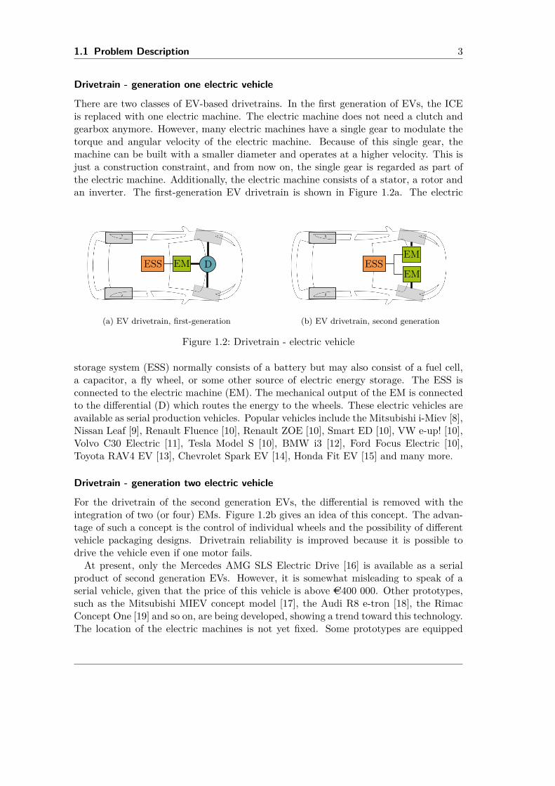
There are two classes of EV-based drivetrains. In the first generation of EVs, the ICEis replaced with one electric machine. The electric machine does not need a clutch andgearbox anymore. However, many electric machines have a single gear to modulate thetorque and angular velocity of the electric machine. Because of this single gear, themachine can be built with a smaller diameter and operates at a higher velocity. This isjust a construction constraint, and from now on, the single gear is regarded as part ofthe electric machine. Additionally, the electric machine consists of a stator, a rotor andan inverter. The first-generation EV drivetrain is shown in Figure 1.2a. The electric
EM DESS
(a) EV drivetrain, first-generation
EM
EMESS
(b) EV drivetrain, second generation
Figure 1.2: Drivetrain - electric vehicle
storage system (ESS) normally consists of a battery but may also consist of a fuel cell,a capacitor, a fly wheel, or some other source of electric energy storage. The ESS isconnected to the electric machine (EM). The mechanical output of the EM is connectedto the differential (D) which routes the energy to the wheels. These electric vehicles areavailable as serial production vehicles. Popular vehicles include the Mitsubishi i-Miev [8],Nissan Leaf [9], Renault Fluence [10], Renault ZOE [10], Smart ED [10], VW e-up! [10],Volvo C30 Electric [11], Tesla Model S [10], BMW i3 [12], Ford Focus Electric [10],Toyota RAV4 EV [13], Chevrolet Spark EV [14], Honda Fit EV [15] and many more.
Drivetrain - generation two electric vehicle
For the drivetrain of the second generation EVs, the differential is removed with theintegration of two (or four) EMs. Figure 1.2b gives an idea of this concept. The advan-tage of such a concept is the control of individual wheels and the possibility of differentvehicle packaging designs. Drivetrain reliability is improved because it is possible todrive the vehicle even if one motor fails.At present, only the Mercedes AMG SLS Electric Drive [16] is available as a serial
product of second generation EVs. However, it is somewhat misleading to speak of aserial vehicle, given that the price of this vehicle is above AC400 000. Other prototypes,such as the Mitsubishi MIEV concept model [17], the Audi R8 e-tron [18], the RimacConcept One [19] and so on, are being developed, showing a trend toward this technology.The location of the electric machines is not yet fixed. Some prototypes are equipped
4 1 Introduction
with hub motors; others are equipped with in-chassis electric machines. Some vehicleshave two motors at the front, some two at the rear, and some even have four motors forevery wheel.
1.2 Scope of Work
This study aims to improve vehicle behaviour by developing a distributed propulsionsystem, driven by two independent electric motors. The safety and performance of thevehicle will be enhanced with a proper controller design. The non-linear, parameter-dependent vehicle dynamics result in a ambitious control problem; in this work thechallenge is addressed within the framework of linear parameter-varying systems, bydeveloping, implementing and testing an LPV controller that is designed to guaran-tee stability and performance. Additionally, the controller will be implemented on anautomotive microcontroller and validated with real test drives.
1.3 Main Objective
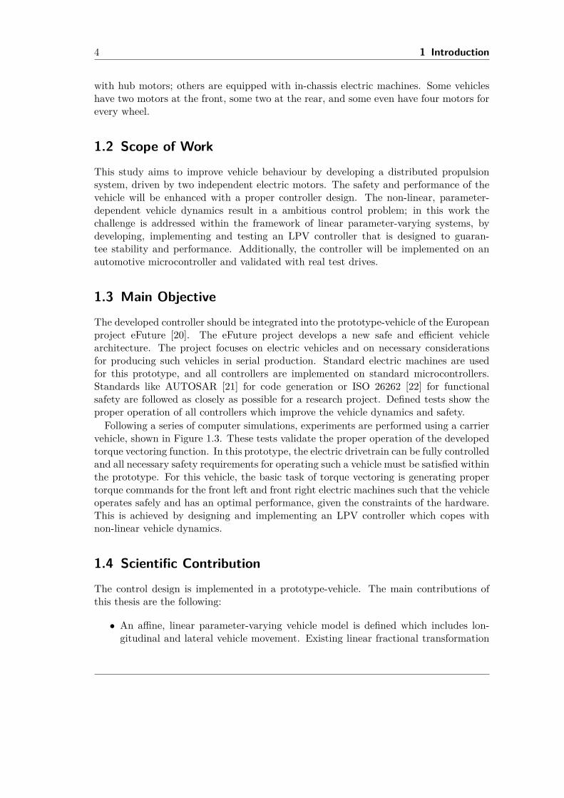
The developed controller should be integrated into the prototype-vehicle of the Europeanproject eFuture [20]. The eFuture project develops a new safe and efficient vehiclearchitecture. The project focuses on electric vehicles and on necessary considerationsfor producing such vehicles in serial production. Standard electric machines are usedfor this prototype, and all controllers are implemented on standard microcontrollers.Standards like AUTOSAR [21] for code generation or ISO 26262 [22] for functionalsafety are followed as closely as possible for a research project. Defined tests show theproper operation of all controllers which improve the vehicle dynamics and safety.Following a series of computer simulations, experiments are performed using a carrier
vehicle, shown in Figure 1.3. These tests validate the proper operation of the developedtorque vectoring function. In this prototype, the electric drivetrain can be fully controlledand all necessary safety requirements for operating such a vehicle must be satisfied withinthe prototype. For this vehicle, the basic task of torque vectoring is generating propertorque commands for the front left and front right electric machines such that the vehicleoperates safely and has an optimal performance, given the constraints of the hardware.This is achieved by designing and implementing an LPV controller which copes withnon-linear vehicle dynamics.
1.4 Scientific Contribution
The control design is implemented in a prototype-vehicle. The main contributions ofthis thesis are the following:
• An affine, linear parameter-varying vehicle model is defined which includes lon-gitudinal and lateral vehicle movement. Existing linear fractional transformation
1.5 Thesis Overview 5
Figure 1.3: Prototype of the eFuture project
and polytopic linear parameter-varying design methods are applied to find linearparameter-varying controllers.
• An existing anti-windup controller design method is applied here to deal withmotor limitations and is extended to meet different vehicle constraints in variousoperating conditions.
• To solve the problem of an underactuated system, the requirements of wheel sliplimitation are integrated into the anti-windup design to achieve a "functionallycontrollable model" [23]. The extension of the anti-windup design to the motortorque and wheel slip limiter is developed.
• A polytopic linear parameter-varying controller for the longitudinal and lateralvehicle dynamics is implemented on an automotive microcontroller.
1.5 Thesis Overview
The rest of the thesis is organised as follows. In Chapter 2, the basic physical relationsand equations for vehicle movement are discussed, especially the planar dynamics thatare relevant for torque vectoring. The general idea of torque vectoring is explainedin detail in Chapter 3. A review of different controller designs and implementationsis provided. In Chapter 4, linear parameter-varying control is briefly explained andapplied to the problem of torque vectoring. Chapter 5 develops an anti-windup concept
6 1 Introduction
to deal with the limitations of the electric drivetrain. This concept is extended tothe motor torque and wheel slip limiter, which also suppresses spinning or locking ofthe driven wheels. Chapter 6 gives an overview of the steps needed to implement thetorque vectoring controller on an automotive microcontroller. Results of test drives arediscussed in Chapter 7. Conclusions and an outlook for future work are given in Chapter8.
2 Automotive Vehicles
To discuss the design of a new torque vectoring controller, more information about ve-hicle dynamics and vehicle components is necessary. A brief account of these topicsis presented in this chapter. Section 2.1 offers an overview of vehicle dynamics andequations to model dynamic vehicle behaviour. Section 2.2 summarises important com-ponents of dynamic vehicle behaviour. Different tyre models are described because tyreshave a major influence on the movement of the vehicle. Additionally, information aboutthe electric drivetrain is provided. Section 2.3 validates different simulation models withmeasurement data obtained during the eFuture project [20].
2.1 Vehicle ModelA vehicle model predicts the behaviour of the vehicle for given changes, inside or outsidethe vehicle. Computer simulations are used for defining and comparing such scenariosunder different conditions. The field of vehicle simulations is used for various investi-gations. For example, crash simulations help to predict the deformation of the vehicleunder certain test scenarios taken from real accidents. Injuries to driver and passengersare made visible and devices to prevent these injuries can be developed. Thermal stresssimulations help to improve the durability of electric components.In the present study, vehicle simulations are related to the movement of the vehicle
with given inputs and disturbances. Inputs to the vehicle are the change of the steeringwheel angle and torques acting on the wheels of the vehicle. Disturbances or externalinputs are the aerodynamic drag forces, the incline of the road, varying road conditionsand so on. A general vehicle model for movement in space is described. Afterwards,reduced models are derived from the general vehicle model, and are used in controllerdesign and controller tuning.
2.1.1 Global vehicle model
For simulating vehicle dynamics, the vehicle is simplified to a single point in space, witha given mass m at the centre of gravity (CoG) and a moment of inertia I. The CoGmoves along three dimensions in space which are described using a coordinate system.As an automotive standard [24] x is defined as the forward direction of the vehicle. Thepositive y direction is to the left side of the vehicle (looking from the top). The positivez direction is to the top side of the vehicle. Besides the three transversal movements,the vehicle rotates along the three axes. Rotation around the x-axis is referred to rollingand is determined by the angle φ. Roation around the y-axis is known as pitch angle θ.Rotation around the vertical z-axis is defined as yaw angle ψ.
7
8 2 Automotive Vehicles
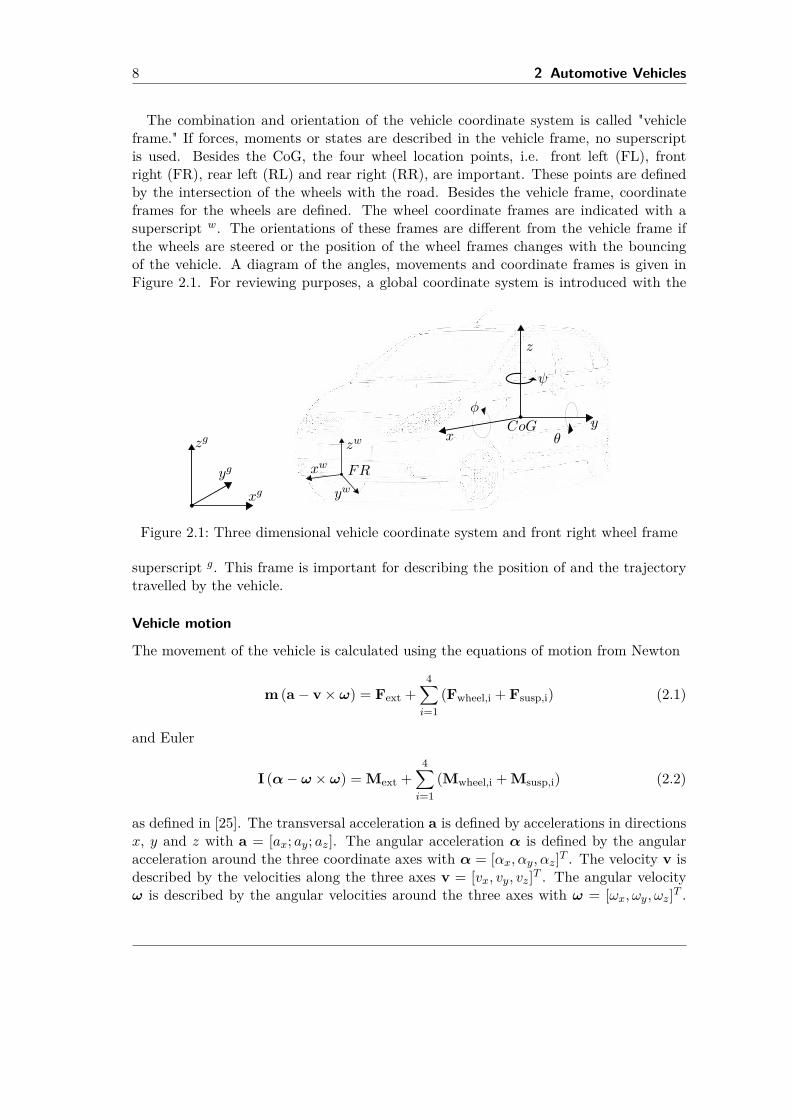
The combination and orientation of the vehicle coordinate system is called "vehicleframe." If forces, moments or states are described in the vehicle frame, no superscriptis used. Besides the CoG, the four wheel location points, i.e. front left (FL), frontright (FR), rear left (RL) and rear right (RR), are important. These points are definedby the intersection of the wheels with the road. Besides the vehicle frame, coordinateframes for the wheels are defined. The wheel coordinate frames are indicated with asuperscript w. The orientations of these frames are different from the vehicle frame ifthe wheels are steered or the position of the wheel frames changes with the bouncingof the vehicle. A diagram of the angles, movements and coordinate frames is given inFigure 2.1. For reviewing purposes, a global coordinate system is introduced with the
xy
z
xw
yw
zwCoG
FR
θ
φ
ψ
zg
yg
xg
Figure 2.1: Three dimensional vehicle coordinate system and front right wheel frame
superscript g. This frame is important for describing the position of and the trajectorytravelled by the vehicle.
Vehicle motion
The movement of the vehicle is calculated using the equations of motion from Newton
m (a − v× ω) = Fext +4∑i=1
(Fwheel,i + Fsusp,i) (2.1)
and Euler
I (α− ω × ω) = Mext +4∑i=1
(Mwheel,i + Msusp,i) (2.2)
as defined in [25]. The transversal acceleration a is defined by accelerations in directionsx, y and z with a = [ax; ay; az]. The angular acceleration α is defined by the angularacceleration around the three coordinate axes with α = [αx, αy, αz]T . The velocity v isdescribed by the velocities along the three axes v = [vx, vy, vz]T . The angular velocityω is described by the angular velocities around the three axes with ω = [ωx, ωy, ωz]T .
2.1 Vehicle Model 9
The CoG changes its movement depending on the forces F = [Fx, Fy, Fz]T and momentsM = [Mx,My,Mz]T which are generated by the wheel forces Fwheel and the suspensionforces Fsusp. Sidewind, gravitational forces and so on act as external forces Fext onthe vehicle. Knowing the forces and the geometric properties of the vehicle, the wheelmoment Mwheel, the suspension moment Msusp and the external moment Mext are cal-culated. The index i is defined as i = 1 for FL, i = 2 for FR, i = 3 for RL and i = 4 forRR.The velocity v and angular velocity ω are defined as
v =∫
a dt+ v0 (2.3)
ω =∫α dt+ ω0 (2.4)
as the integrals of the acceleration and angular acceleration, where v0 represents theinitial velocity and ω0 the initial angular velocity.For the torque vectoring development, it is sufficient to calculate (2.1 - 2.4). These
equations describe the vehicle forces and their effects on the vehicle velocity. For vi-sualisation, or other vehicle controllers like active cruise control, it is advantageous tocalculate the position p of the vehicle in the global coordinate frame pg = [pgx, pgy, pgz]. Tocalculate the global vehicle position pg, the velocity of the vehicle v is described in theglobal coordinate frame as vg with the transformation matrix T. Similarly, the globalvehicle angle Φg = [φg, θg, ψg] is calculated from the angular velocity ω of the vehiclewhich is represented in the global coordinate system as ωg. The transformation matrixTg from the vehicle to the global frame is defined as
Tg =
cosψg sinψg 0− sinψg cosψg 0
0 0 1
cos θg 0 − sin θg
0 1 0sin θg 0 cos θg
1 0 0
0 cosφg sinφg0 − sinφg cosφg
. (2.5)
In the global frame the velocity and angular velocity are defined as
vg = Tgvωg = Tgω.
(2.6)
For the transformation matrices T, the superscript indicates the new coordinate systemwhere the subscript defines the actual coordinate system. Tg defines the transformationfrom the vehicle coordinate system to the global coordinate system.Integrating the velocity vg and angular velocity ωg over the time t defines the global
position pg and angle Φg as
pg =∫
vg dt+ pg0 (2.7)
Φg =∫ωg dt+ Φg
0, (2.8)
10 2 Automotive Vehicles
where pg0 defines the initial vehicle position and Φg0 describes the initial vehicle angle in
the global frame.
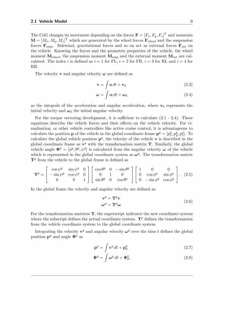
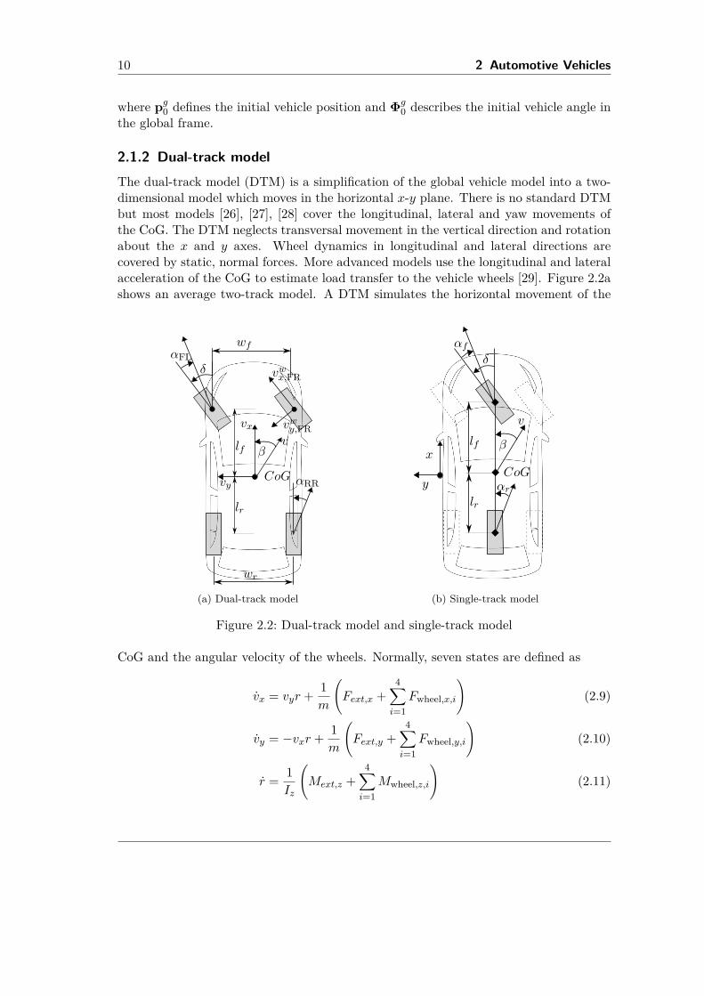
2.1.2 Dual-track modelThe dual-track model (DTM) is a simplification of the global vehicle model into a two-dimensional model which moves in the horizontal x-y plane. There is no standard DTMbut most models [26], [27], [28] cover the longitudinal, lateral and yaw movements ofthe CoG. The DTM neglects transversal movement in the vertical direction and rotationabout the x and y axes. Wheel dynamics in longitudinal and lateral directions arecovered by static, normal forces. More advanced models use the longitudinal and lateralacceleration of the CoG to estimate load transfer to the vehicle wheels [29]. Figure 2.2ashows an average two-track model. A DTM simulates the horizontal movement of the
β
δ
lr
lf
CoG
v
vx
vy αRR
αFLvwx,FR
vwy,FR
wr
wf
(a) Dual-track model
β
δ
lr
lf
CoG
v
x
y αr
αf
(b) Single-track model
Figure 2.2: Dual-track model and single-track model
CoG and the angular velocity of the wheels. Normally, seven states are defined as
vx = vyr + 1m
(Fext,x +
4∑i=1
Fwheel,x,i
)(2.9)
vy = −vxr + 1m
(Fext,y +
4∑i=1
Fwheel,y,i
)(2.10)
r = 1Iz
(Mext,z +
4∑i=1
Mwheel,z,i
)(2.11)
2.1 Vehicle Model 11
ωi = 1Iw
(Ti −RiF gx,i
), (2.12)
where the states are represented with the longitudinal velocity vx, the lateral velocityvy, the yaw rate r and the angular velocities of the four wheels ωi. The longitudinal tyreforces Fx,i, the lateral tyre forces Fy,i and the restoring moment Mz,i of the tyres acton the vehicle. The external forces Fx,ext in the longitudinal direction, Fy,ext in lateraldirection and the external moment Mz,ext are additional disturbances to the vehicle’smovement. External forces are related to air-drag, tyre-friction, trailer operation andso on. The mass m represents the weight of the vehicle. The vehicle moment of inertiaaround the vertical axis is described by Iz and the wheel moment of inertia around thespinning wheel axis is labelled Iw. The effective roll radius of the tyre R is defined as thedistance from the road contact point to the centre point of the wheel. The tyre model isnot fixed for the two-track model. The longitudinal tyre force Fx,wheel, the lateral tyreforce Fy,wheel and tyre yaw moment Mz,wheel depend mainly on the longitudinal velocityof the vehicle vx, the wheel slip λ, the tyre slip angle α, the road surface conditionsµ and the vertical tyre load Fz,wheel. Different tyre models have been developed, andthe accuracy of the calculation of tyre forces has a major effect on the quality of thetwo-track model. A detailed explanation of the tyre models is given in Section 2.2.1.
2.1.3 Single-track model
The single-track model (STM) is the most common model in the literature [25], [30], [31],[32] for lateral vehicle control. The basic idea of the STM is to merge both wheels ofan axle into a single wheel. This idea is shown in Figure 2.2b. The model assumes thatthe left and right wheels generate the same lateral forces. The lateral force generationis linear to the combined tyre slip angle α. The longitudinal tyre force generation iscombined to a general, longitudinal input force Fx. The STM is non-linear but can belinearised for a certain longitudinal velocity vx0 . Here, the STM expects that the tyreslip λ and tyre slip angle α are limited and in the range of |λ| < 0.15 and |α| < 0.1 rad.Furthermore, the vehicle must drive forward with vx > 1kph to achieve numericallystable results. For reverse driving the equations (2.13 - 2.15) or (2.17 - 2.18) must bemodified; see [25] for more details. The linear and non-linear vehicle models are regardedas front steering vehicles with additional devices, required to apply a yaw moment Mz.
Non-linear single-track model
The non-linear model is defined as
vx = vyr + 1mFx (2.13)
vy = −Cy,F + Cy,Rmvx
vy +(−lFCy,F + lRCy,R
mvx− vx
)r + Cy,F
mδ (2.14)
r = −lFCy,F + lRCy,RIzvx
vy −l2FCy,F + l2RCy,R
Izvxr + lFCy,F
Izδ + 1
IzMz. (2.15)
12 2 Automotive Vehicles
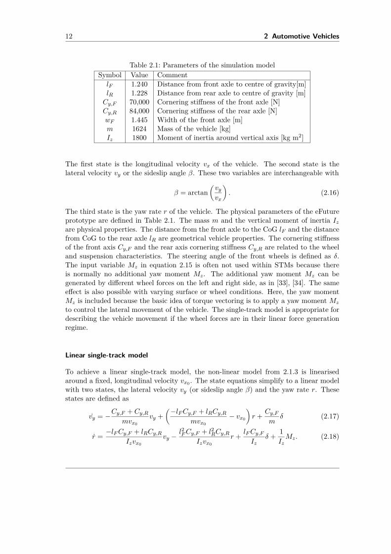
Table 2.1: Parameters of the simulation modelSymbol Value CommentlF 1.240 Distance from front axle to centre of gravity[m]lR 1.228 Distance from rear axle to centre of gravity [m]Cy,F 70,000 Cornering stiffness of the front axle [N]Cy,R 84,000 Cornering stiffness of the rear axle [N]wF 1.445 Width of the front axle [m]m 1624 Mass of the vehicle [kg]Iz 1800 Moment of inertia around vertical axis [kg m2]
The first state is the longitudinal velocity vx of the vehicle. The second state is thelateral velocity vy or the sideslip angle β. These two variables are interchangeable with
β = arctan(vyvx
). (2.16)
The third state is the yaw rate r of the vehicle. The physical parameters of the eFutureprototype are defined in Table 2.1. The mass m and the vertical moment of inertia Izare physical properties. The distance from the front axle to the CoG lF and the distancefrom CoG to the rear axle lR are geometrical vehicle properties. The cornering stiffnessof the front axis Cy,F and the rear axis cornering stiffness Cy,R are related to the wheeland suspension characteristics. The steering angle of the front wheels is defined as δ.The input variable Mz in equation 2.15 is often not used within STMs because thereis normally no additional yaw moment Mz. The additional yaw moment Mz can begenerated by different wheel forces on the left and right side, as in [33], [34]. The sameeffect is also possible with varying surface or wheel conditions. Here, the yaw momentMz is included because the basic idea of torque vectoring is to apply a yaw moment Mz
to control the lateral movement of the vehicle. The single-track model is appropriate fordescribing the vehicle movement if the wheel forces are in their linear force generationregime.
Linear single-track model
To achieve a linear single-track model, the non-linear model from 2.1.3 is linearisedaround a fixed, longitudinal velocity vx0 . The state equations simplify to a linear modelwith two states, the lateral velocity vy (or sideslip angle β) and the yaw rate r. Thesestates are defined as
vy = −Cy,F + Cy,Rmvx0
vy +(−lFCy,F + lRCy,R
mvx0− vx0
)r + Cy,F
mδ (2.17)
r = −lFCy,F + lRCy,RIzvx0
vy −l2FCy,F + l2RCy,R
Izvx0r + lFCy,F
Izδ + 1
IzMz. (2.18)
2.2 Vehicle Components 13
The inputs to the linear STM are the steering angle of the front wheels δ and the yawmoment Mz. The parameters of the model are defined in Table 2.1.
2.2 Vehicle Components
As mentioned before, the simulation of the vehicle dynamics relies on the physical lawsof Newton and Euler. Therefore, the generated wheel forces acting on the chassis mustbe calculated. The resulting wheel forces are influenced by the propulsion system, thewheel steering and external forces. These components will be briefly discussed in thenext section.
2.2.1 Wheels
The wheel tyres are one of the most important components for vehicle dynamics becausethe wheels are the vehicle’s connection to the ground. The wheels have to fulfil varioustasks. Firstly, wheels act as springs and dampers for the vehicle. Secondly, wheelsgenerate longitudinal and lateral forces to manoeuvre the vehicle. To accelerate orbrake the vehicle, a torque T is applied to the wheel through the electric motor or thehydraulic brake. The torque acting on the wheel changes the angular acceleration ω ofthe wheel and hence the movement of the wheel. This relationship is defined as
ω = 1Iw
(T − Fwx R) , (2.19)
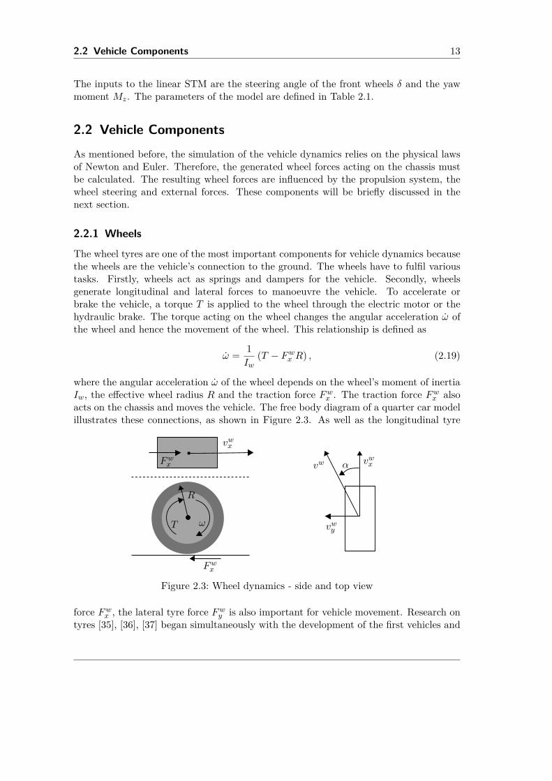
where the angular acceleration ω of the wheel depends on the wheel’s moment of inertiaIw, the effective wheel radius R and the traction force Fwx . The traction force Fwx alsoacts on the chassis and moves the vehicle. The free body diagram of a quarter car modelillustrates these connections, as shown in Figure 2.3. As well as the longitudinal tyre
vwx
T
Fwx
ω
vwx
vwy
αvwFwx
R
Figure 2.3: Wheel dynamics - side and top view
force Fwx , the lateral tyre force Fwy is also important for vehicle movement. Research ontyres [35], [36], [37] began simultaneously with the development of the first vehicles and
14 2 Automotive Vehicles
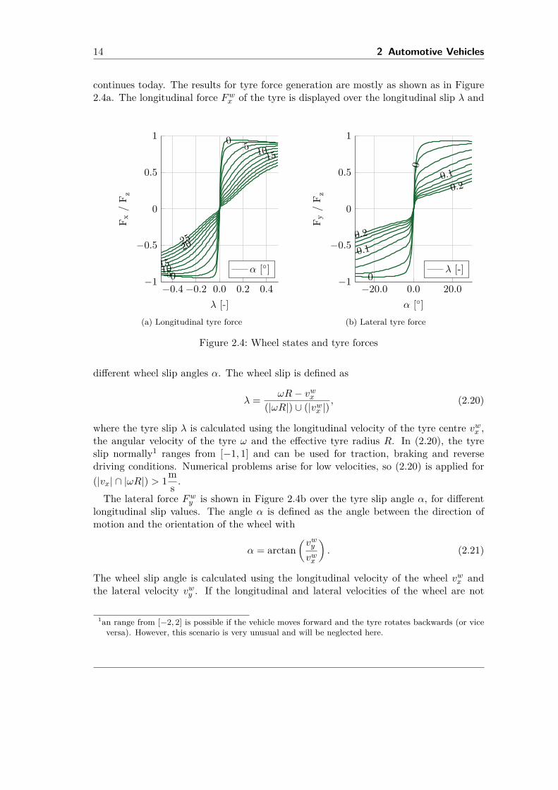
continues today. The results for tyre force generation are mostly as shown as in Figure2.4a. The longitudinal force Fwx of the tyre is displayed over the longitudinal slip λ and
−0.4 −0.2 0.0 0.2 0.4−1
−0.5
0
0.5
1 0
0
5
5
10
10
15
152025
λ [-]
F x/
F z
α []
(a) Longitudinal tyre force
−20.0 0.0 20.0−1
−0.5
0
0.5
1
0
0
0.1
0.1
0.2
0.2
α []F y
/F z
λ [-]
(b) Lateral tyre force
Figure 2.4: Wheel states and tyre forces
different wheel slip angles α. The wheel slip is defined as
λ = ωR− vwx(|ωR|) ∪ (|vwx |)
, (2.20)
where the tyre slip λ is calculated using the longitudinal velocity of the tyre centre vwx ,the angular velocity of the tyre ω and the effective tyre radius R. In (2.20), the tyreslip normally1 ranges from [−1, 1] and can be used for traction, braking and reversedriving conditions. Numerical problems arise for low velocities, so (2.20) is applied for(|vx| ∩ |ωR|) > 1ms .The lateral force Fwy is shown in Figure 2.4b over the tyre slip angle α, for different
longitudinal slip values. The angle α is defined as the angle between the direction ofmotion and the orientation of the wheel with
α = arctan(vwyvwx
). (2.21)
The wheel slip angle is calculated using the longitudinal velocity of the wheel vwx andthe lateral velocity vwy . If the longitudinal and lateral velocities of the wheel are not
1an range from [−2, 2] is possible if the vehicle moves forward and the tyre rotates backwards (or viceversa). However, this scenario is very unusual and will be neglected here.
2.2 Vehicle Components 15
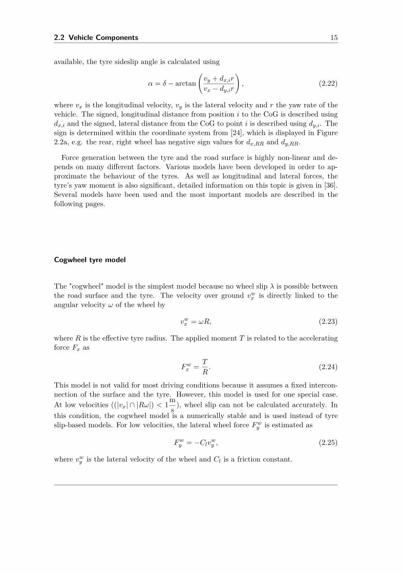
available, the tyre sideslip angle is calculated using
α = δ − arctan(vy + dx,ir
vx − dy,ir
), (2.22)
where vx is the longitudinal velocity, vy is the lateral velocity and r the yaw rate of thevehicle. The signed, longitudinal distance from position i to the CoG is described usingdx,i and the signed, lateral distance from the CoG to point i is described using dy,i. Thesign is determined within the coordinate system from [24], which is displayed in Figure2.2a, e.g. the rear, right wheel has negative sign values for dx,RR and dy,RR.
Force generation between the tyre and the road surface is highly non-linear and de-pends on many different factors. Various models have been developed in order to ap-proximate the behaviour of the tyres. As well as longitudinal and lateral forces, thetyre’s yaw moment is also significant, detailed information on this topic is given in [36].Several models have been used and the most important models are described in thefollowing pages.
Cogwheel tyre model
The "cogwheel" model is the simplest model because no wheel slip λ is possible betweenthe road surface and the tyre. The velocity over ground vwx is directly linked to theangular velocity ω of the wheel by
vwx = ωR, (2.23)
where R is the effective tyre radius. The applied moment T is related to the acceleratingforce Fx as
Fwx = T
R. (2.24)
This model is not valid for most driving conditions because it assumes a fixed intercon-nection of the surface and the tyre. However, this model is used for one special case.At low velocities ((|vx| ∩ |Rω|) < 1ms ), wheel slip can not be calculated accurately. Inthis condition, the cogwheel model is a numerically stable and is used instead of tyreslip-based models. For low velocities, the lateral wheel force Fwy is estimated as
Fwy = −Clvwy , (2.25)
where vwy is the lateral velocity of the wheel and Cl is a friction constant.
16 2 Automotive Vehicles
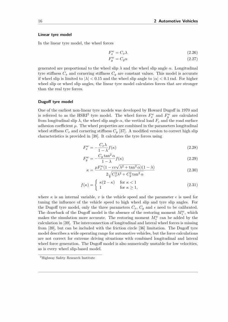
Linear tyre model
In the linear tyre model, the wheel forces
Fwx = Cxλ (2.26)Fwy = Cyα (2.27)
generated are proportional to the wheel slip λ and the wheel slip angle α. Longitudinaltyre stiffness Cx and cornering stiffness Cy are constant values. This model is accurateif wheel slip is limited to |λ| < 0.15 and the wheel slip angle to |α| < 0.1 rad. For higherwheel slip or wheel slip angles, the linear tyre model calculates forces that are strongerthan the real tyre forces.
Dugoff tyre model
One of the earliest non-linear tyre models was developed by Howard Dugoff in 1970 andis referred to as the HSRI2 tyre model. The wheel forces Fwx and Fwy are calculatedfrom longitudinal slip λ, the wheel slip angle α, the vertical load Fz and the road surfaceadhesion coefficient µ. The wheel properties are combined in the parameters longitudinalwheel stiffness Cx and cornering stiffness Cy [37]. A modified version to correct high slipcharacteristics is provided in [38]. It calculates the tyre forces using
Fwx = − Cxλ
1− λf(κ) (2.28)
Fwy = −Cy tan2 α
1− λ f(κ) (2.29)
κ = µFwz (1− εv√λ2 + tan2 α)(1− λ)
2√C2xλ
2 + C2y tan2 α
(2.30)
f(κ) =κ(2− κ) for κ < 11 for κ ≥ 1, (2.31)
where κ is an internal variable, v is the vehicle speed and the parameter ε is used fortuning the influence of the vehicle speed to high wheel slip and tyre slip angles. Forthe Dugoff tyre model, only the three parameters Cx, Cy and ε need to be calibrated.The drawback of the Dugoff model is the absence of the restoring moment Mw
z , whichmakes the simulation more accurate. The restoring moment Mw
z can be added by thecalculation in [39]. The interconnection of longitudinal and lateral wheel forces is missingfrom [39], but can be included with the friction circle [36] limitation. The Dugoff tyremodel describes a wide operating range for automotive vehicles, but the force calculationsare not correct for extreme driving situations with combined longitudinal and lateralwheel force generation. The Dugoff model is also numerically unstable for low velocities,as is every wheel slip-based model.
2Highway Safety Research Institute
2.2 Vehicle Components 17
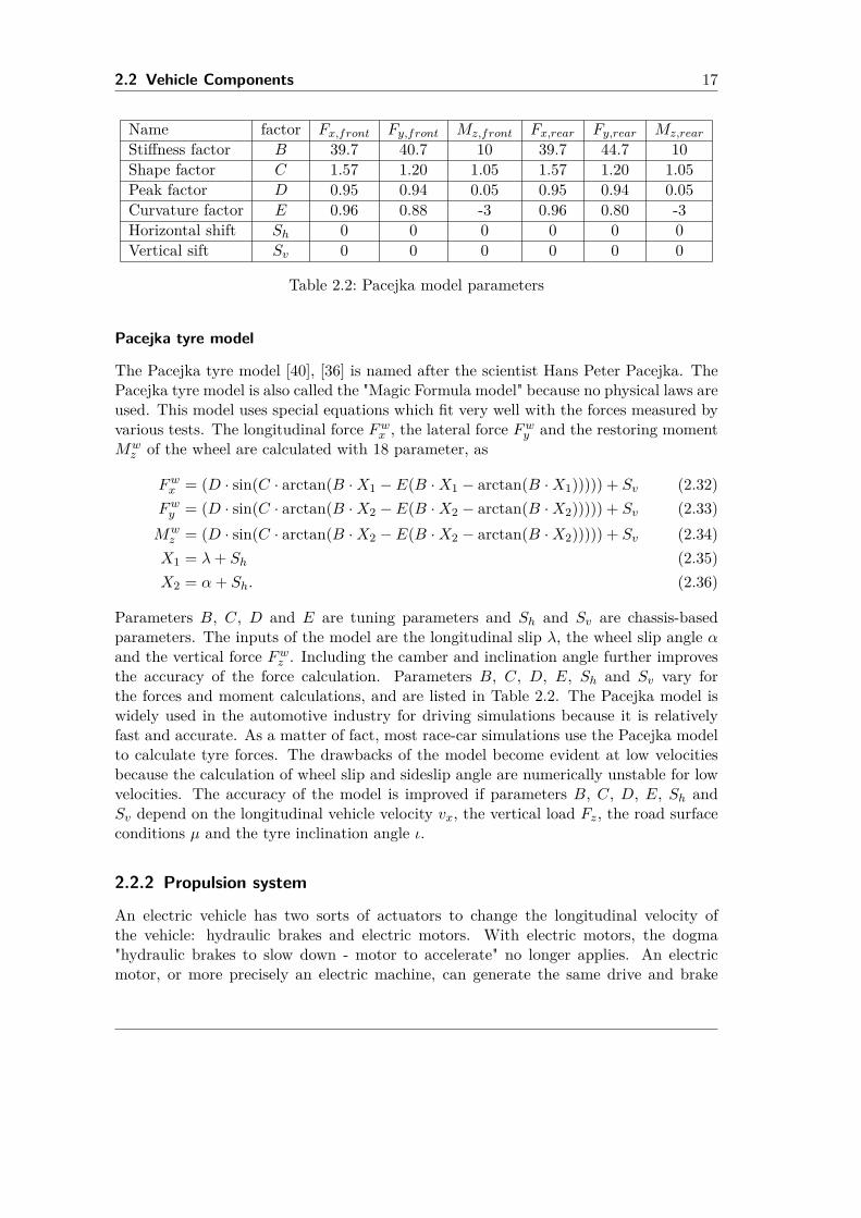
Name factor Fx,front Fy,front Mz,front Fx,rear Fy,rear Mz,rear
Stiffness factor B 39.7 40.7 10 39.7 44.7 10Shape factor C 1.57 1.20 1.05 1.57 1.20 1.05Peak factor D 0.95 0.94 0.05 0.95 0.94 0.05Curvature factor E 0.96 0.88 -3 0.96 0.80 -3Horizontal shift Sh 0 0 0 0 0 0Vertical sift Sv 0 0 0 0 0 0
Table 2.2: Pacejka model parameters
Pacejka tyre model
The Pacejka tyre model [40], [36] is named after the scientist Hans Peter Pacejka. ThePacejka tyre model is also called the "Magic Formula model" because no physical laws areused. This model uses special equations which fit very well with the forces measured byvarious tests. The longitudinal force Fwx , the lateral force Fwy and the restoring momentMwz of the wheel are calculated with 18 parameter, as
Fwx = (D · sin(C · arctan(B ·X1 − E(B ·X1 − arctan(B ·X1))))) + Sv (2.32)Fwy = (D · sin(C · arctan(B ·X2 − E(B ·X2 − arctan(B ·X2))))) + Sv (2.33)Mwz = (D · sin(C · arctan(B ·X2 − E(B ·X2 − arctan(B ·X2))))) + Sv (2.34)X1 = λ+ Sh (2.35)X2 = α+ Sh. (2.36)
Parameters B, C, D and E are tuning parameters and Sh and Sv are chassis-basedparameters. The inputs of the model are the longitudinal slip λ, the wheel slip angle αand the vertical force Fwz . Including the camber and inclination angle further improvesthe accuracy of the force calculation. Parameters B, C, D, E, Sh and Sv vary forthe forces and moment calculations, and are listed in Table 2.2. The Pacejka model iswidely used in the automotive industry for driving simulations because it is relativelyfast and accurate. As a matter of fact, most race-car simulations use the Pacejka modelto calculate tyre forces. The drawbacks of the model become evident at low velocitiesbecause the calculation of wheel slip and sideslip angle are numerically unstable for lowvelocities. The accuracy of the model is improved if parameters B, C, D, E, Sh andSv depend on the longitudinal vehicle velocity vx, the vertical load Fz, the road surfaceconditions µ and the tyre inclination angle ι.
2.2.2 Propulsion system
An electric vehicle has two sorts of actuators to change the longitudinal velocity ofthe vehicle: hydraulic brakes and electric motors. With electric motors, the dogma"hydraulic brakes to slow down - motor to accelerate" no longer applies. An electricmotor, or more precisely an electric machine, can generate the same drive and brake
18 2 Automotive Vehicles
torque. The only difference is that for acceleration the battery has to provide electricenergy to the electric machines. The machines act as motors and convert electricalenergy to mechanical energy. In the case of electrical deceleration, the electric machinesact as generators and convert mechanical energy into electrical energy. The electricalenergy generated is routed to the battery and charges the battery. The electric brakingprocess is referred to as recuperation.
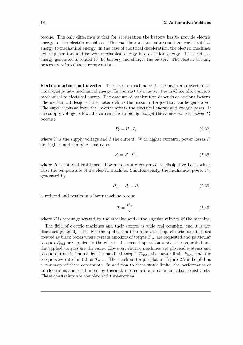
Electric machine and inverter The electric machine with the inverter converts elec-trical energy into mechanical energy. In contrast to a motor, the machine also convertsmechanical to electrical energy. The amount of acceleration depends on various factors.The mechanical design of the motor defines the maximal torque that can be generated.The supply voltage from the inverter affects the electrical energy and energy losses. Ifthe supply voltage is low, the current has to be high to get the same electrical power Pebecause
Pe = U · I, (2.37)
where U is the supply voltage and I the current. With higher currents, power losses Plare higher, and can be estimated as
Pl = R · I2, (2.38)
where R is internal resistance. Power losses are converted to dissipative heat, whichraise the temperature of the electric machine. Simultaneously, the mechanical power Pmgenerated by
Pm = Pe − Pl (2.39)
is reduced and results in a lower machine torque
T = Pmω, (2.40)
where T is torque generated by the machine and ω the angular velocity of the machine.The field of electric machines and their control is wide and complex, and it is not
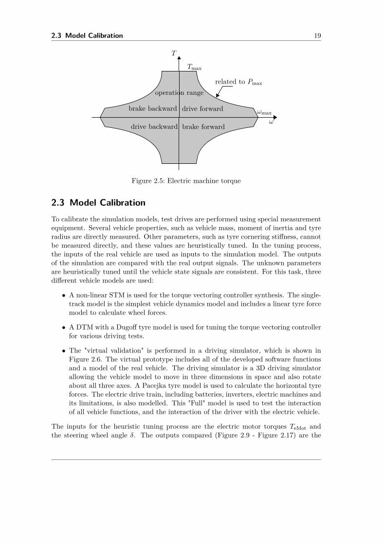
discussed generally here. For the application to torque vectoring, electric machines aretreated as black boxes where certain amounts of torque Treq are requested and particulartorques Treal are applied to the wheels. In normal operation mode, the requested andthe applied torques are the same. However, electric machines are physical systems andtorque output is limited by the maximal torque Tmax, the power limit Pmax and thetorque slew rate limitation Tmax. The machine torque plot in Figure 2.5 is helpful asa summary of these constraints. In addition to these static limits, the performance ofan electric machine is limited by thermal, mechanical and communication constraints.These constraints are complex and time-varying.
2.3 Model Calibration 19
ω
T
Tmax
related to Pmax
drive forward
brake forwarddrive backward
brake backward ωmax
operation range
Figure 2.5: Electric machine torque
2.3 Model CalibrationTo calibrate the simulation models, test drives are performed using special measurementequipment. Several vehicle properties, such as vehicle mass, moment of inertia and tyreradius are directly measured. Other parameters, such as tyre cornering stiffness, cannotbe measured directly, and these values are heuristically tuned. In the tuning process,the inputs of the real vehicle are used as inputs to the simulation model. The outputsof the simulation are compared with the real output signals. The unknown parametersare heuristically tuned until the vehicle state signals are consistent. For this task, threedifferent vehicle models are used:
• A non-linear STM is used for the torque vectoring controller synthesis. The single-track model is the simplest vehicle dynamics model and includes a linear tyre forcemodel to calculate wheel forces.
• A DTM with a Dugoff tyre model is used for tuning the torque vectoring controllerfor various driving tests.
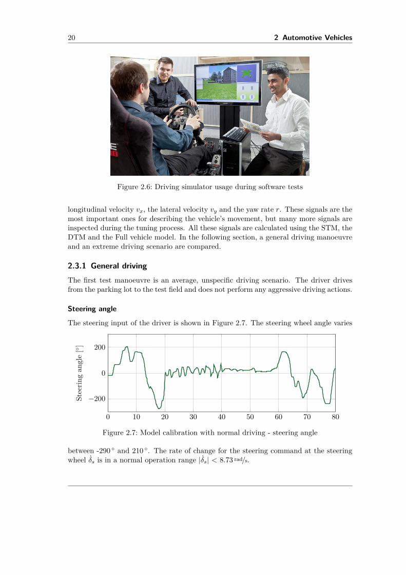
• The "virtual validation" is performed in a driving simulator, which is shown inFigure 2.6. The virtual prototype includes all of the developed software functionsand a model of the real vehicle. The driving simulator is a 3D driving simulatorallowing the vehicle model to move in three dimensions in space and also rotateabout all three axes. A Pacejka tyre model is used to calculate the horizontal tyreforces. The electric drive train, including batteries, inverters, electric machines andits limitations, is also modelled. This "Full" model is used to test the interactionof all vehicle functions, and the interaction of the driver with the electric vehicle.
The inputs for the heuristic tuning process are the electric motor torques TeMot andthe steering wheel angle δ. The outputs compared (Figure 2.9 - Figure 2.17) are the
20 2 Automotive Vehicles
Figure 2.6: Driving simulator usage during software tests
longitudinal velocity vx, the lateral velocity vy and the yaw rate r. These signals are themost important ones for describing the vehicle’s movement, but many more signals areinspected during the tuning process. All these signals are calculated using the STM, theDTM and the Full vehicle model. In the following section, a general driving manoeuvreand an extreme driving scenario are compared.
2.3.1 General drivingThe first test manoeuvre is an average, unspecific driving scenario. The driver drivesfrom the parking lot to the test field and does not perform any aggressive driving actions.
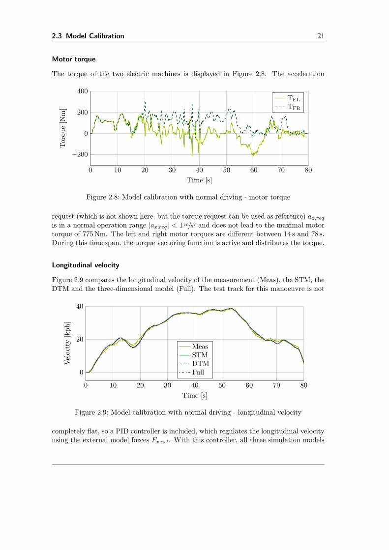
Steering angle
The steering input of the driver is shown in Figure 2.7. The steering wheel angle varies
0 10 20 30 40 50 60 70 80
−200
0
200
Stee
ring
angl
e[ ]
Figure 2.7: Model calibration with normal driving - steering angle
between -290 and 210 . The rate of change for the steering command at the steeringwheel δs is in a normal operation range |δs| < 8.73 rad/s.
2.3 Model Calibration 21
Motor torque
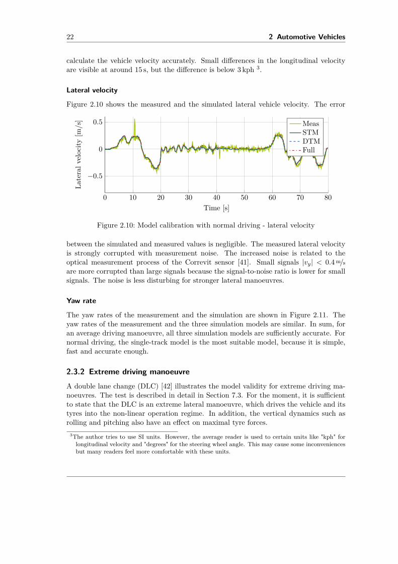
The torque of the two electric machines is displayed in Figure 2.8. The acceleration
0 10 20 30 40 50 60 70 80
−200
0
200
400
Time [s]
Torq
ue[N
m]
TFLTFR
Figure 2.8: Model calibration with normal driving - motor torque
request (which is not shown here, but the torque request can be used as reference) ax,reqis in a normal operation range |ax,req| < 1m/s2 and does not lead to the maximal motortorque of 775Nm. The left and right motor torques are different between 14 s and 78 s.During this time span, the torque vectoring function is active and distributes the torque.
Longitudinal velocity
Figure 2.9 compares the longitudinal velocity of the measurement (Meas), the STM, theDTM and the three-dimensional model (Full). The test track for this manoeuvre is not
0 10 20 30 40 50 60 70 80
0
20
40
Time [s]
Velo
city
[kph
]
MeasSTMDTMFull
Figure 2.9: Model calibration with normal driving - longitudinal velocity
completely flat, so a PID controller is included, which regulates the longitudinal velocityusing the external model forces Fx,ext. With this controller, all three simulation models
22 2 Automotive Vehicles
calculate the vehicle velocity accurately. Small differences in the longitudinal velocityare visible at around 15 s, but the difference is below 3 kph 3.
Lateral velocity
Figure 2.10 shows the measured and the simulated lateral vehicle velocity. The error
0 10 20 30 40 50 60 70 80
−0.5
0
0.5
Time [s]
Late
ralv
eloc
ity[m
/s] Meas
STMDTMFull
Figure 2.10: Model calibration with normal driving - lateral velocity
between the simulated and measured values is negligible. The measured lateral velocityis strongly corrupted with measurement noise. The increased noise is related to theoptical measurement process of the Correvit sensor [41]. Small signals |vy| < 0.4 m/sare more corrupted than large signals because the signal-to-noise ratio is lower for smallsignals. The noise is less disturbing for stronger lateral manoeuvres.
Yaw rate
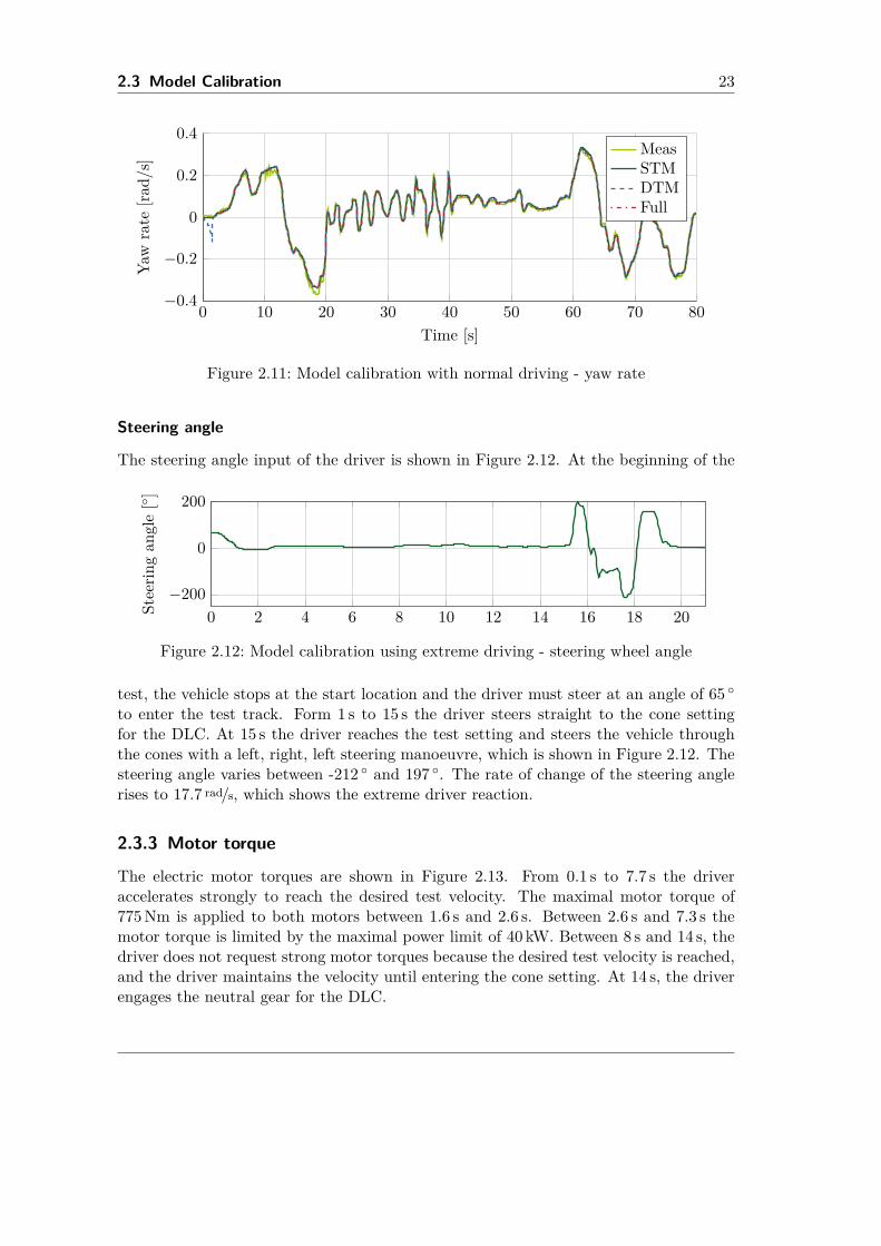
The yaw rates of the measurement and the simulation are shown in Figure 2.11. Theyaw rates of the measurement and the three simulation models are similar. In sum, foran average driving manoeuvre, all three simulation models are sufficiently accurate. Fornormal driving, the single-track model is the most suitable model, because it is simple,fast and accurate enough.
2.3.2 Extreme driving manoeuvre
A double lane change (DLC) [42] illustrates the model validity for extreme driving ma-noeuvres. The test is described in detail in Section 7.3. For the moment, it is sufficientto state that the DLC is an extreme lateral manoeuvre, which drives the vehicle and itstyres into the non-linear operation regime. In addition, the vertical dynamics such asrolling and pitching also have an effect on maximal tyre forces.
3The author tries to use SI units. However, the average reader is used to certain units like "kph" forlongitudinal velocity and "degrees" for the steering wheel angle. This may cause some inconveniencesbut many readers feel more comfortable with these units.
2.3 Model Calibration 23
0 10 20 30 40 50 60 70 80−0.4
−0.2
0
0.2
0.4
Time [s]
Yaw
rate
[rad/
s]MeasSTMDTMFull
Figure 2.11: Model calibration with normal driving - yaw rate
Steering angle
The steering angle input of the driver is shown in Figure 2.12. At the beginning of the
0 2 4 6 8 10 12 14 16 18 20−200
0
200
Stee
ring
angl
e[ ]
Figure 2.12: Model calibration using extreme driving - steering wheel angle
test, the vehicle stops at the start location and the driver must steer at an angle of 65 to enter the test track. Form 1 s to 15 s the driver steers straight to the cone settingfor the DLC. At 15 s the driver reaches the test setting and steers the vehicle throughthe cones with a left, right, left steering manoeuvre, which is shown in Figure 2.12. Thesteering angle varies between -212 and 197 . The rate of change of the steering anglerises to 17.7 rad/s, which shows the extreme driver reaction.
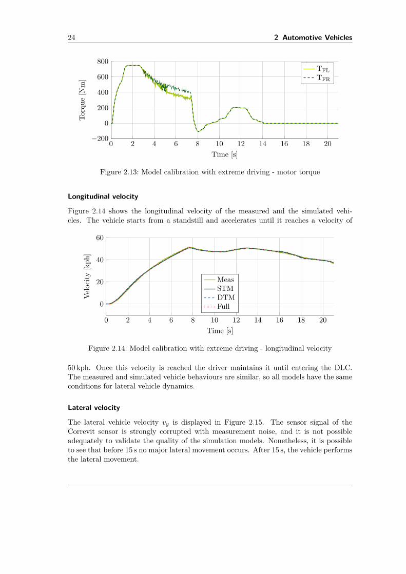
2.3.3 Motor torque
The electric motor torques are shown in Figure 2.13. From 0.1 s to 7.7 s the driveraccelerates strongly to reach the desired test velocity. The maximal motor torque of775Nm is applied to both motors between 1.6 s and 2.6 s. Between 2.6 s and 7.3 s themotor torque is limited by the maximal power limit of 40 kW. Between 8 s and 14 s, thedriver does not request strong motor torques because the desired test velocity is reached,and the driver maintains the velocity until entering the cone setting. At 14 s, the driverengages the neutral gear for the DLC.
24 2 Automotive Vehicles
0 2 4 6 8 10 12 14 16 18 20−200
0
200
400
600
800
Time [s]
Torq
ue[N
m]
TFLTFR
Figure 2.13: Model calibration with extreme driving - motor torque
Longitudinal velocity
Figure 2.14 shows the longitudinal velocity of the measured and the simulated vehi-cles. The vehicle starts from a standstill and accelerates until it reaches a velocity of
0 2 4 6 8 10 12 14 16 18 20
0
20
40
60
Time [s]
Velo
city
[kph
]
MeasSTMDTMFull
Figure 2.14: Model calibration with extreme driving - longitudinal velocity
50 kph. Once this velocity is reached the driver maintains it until entering the DLC.The measured and simulated vehicle behaviours are similar, so all models have the sameconditions for lateral vehicle dynamics.
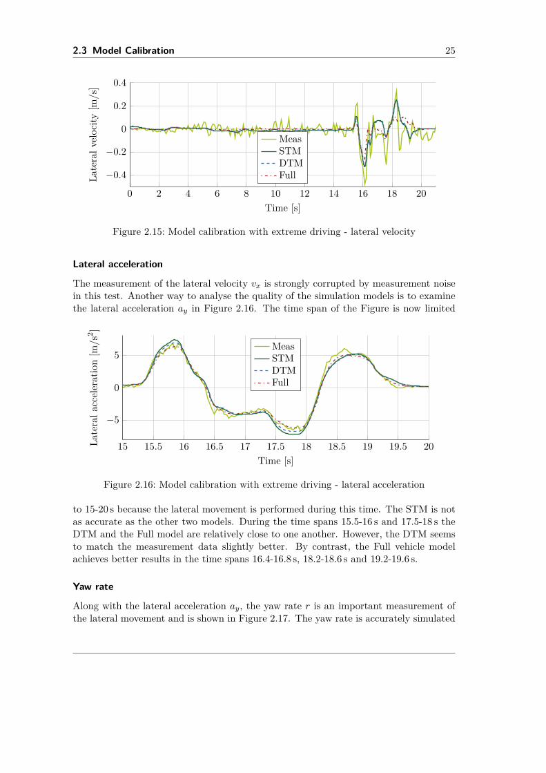
Lateral velocity
The lateral vehicle velocity vy is displayed in Figure 2.15. The sensor signal of theCorrevit sensor is strongly corrupted with measurement noise, and it is not possibleadequately to validate the quality of the simulation models. Nonetheless, it is possibleto see that before 15 s no major lateral movement occurs. After 15 s, the vehicle performsthe lateral movement.
2.3 Model Calibration 25
0 2 4 6 8 10 12 14 16 18 20
−0.4
−0.2
0
0.2
0.4
Time [s]
Late
ralv
eloc
ity[m
/s]
MeasSTMDTMFull
Figure 2.15: Model calibration with extreme driving - lateral velocity
Lateral acceleration
The measurement of the lateral velocity vx is strongly corrupted by measurement noisein this test. Another way to analyse the quality of the simulation models is to examinethe lateral acceleration ay in Figure 2.16. The time span of the Figure is now limited
15 15.5 16 16.5 17 17.5 18 18.5 19 19.5 20
−5
0
5
Time [s]
Late
rala
ccel
erat
ion
[m/s
2 ]
MeasSTMDTMFull
Figure 2.16: Model calibration with extreme driving - lateral acceleration
to 15-20 s because the lateral movement is performed during this time. The STM is notas accurate as the other two models. During the time spans 15.5-16 s and 17.5-18 s theDTM and the Full model are relatively close to one another. However, the DTM seemsto match the measurement data slightly better. By contrast, the Full vehicle modelachieves better results in the time spans 16.4-16.8 s, 18.2-18.6 s and 19.2-19.6 s.
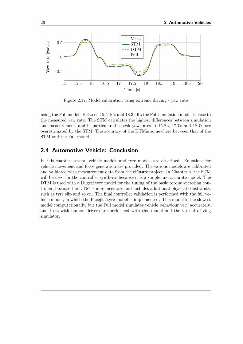
Yaw rate
Along with the lateral acceleration ay, the yaw rate r is an important measurement ofthe lateral movement and is shown in Figure 2.17. The yaw rate is accurately simulated
26 2 Automotive Vehicles
15 15.5 16 16.5 17 17.5 18 18.5 19 19.5 20
−0.5
0
0.5
Time [s]
Yaw
rate
[rad/
s]
MeasSTMDTMFull
Figure 2.17: Model calibration using extreme driving - yaw rate
using the Full model. Between 15.5-16 s and 18.3-19 s the Full simulation model is close tothe measured yaw rate. The STM calculates the highest differences between simulationand measurement, and in particular the peak yaw rates at 15.8 s, 17.7 s and 18.7 s areoverestimated by the STM. The accuracy of the DTMis somewhere between that of theSTM and the Full model.
2.4 Automotive Vehicle: ConclusionIn this chapter, several vehicle models and tyre models are described. Equations forvehicle movement and force generation are provided. The various models are calibratedand validated with measurement data from the eFuture project. In Chapter 4, the STMwill be used for the controller synthesis because it is a simple and accurate model. TheDTM is used with a Dugoff tyre model for the tuning of the basic torque vectoring con-troller, because the DTM is more accurate and includes additional physical constraints,such as tyre slip and so on. The final controller validation is performed with the full ve-hicle model, in which the Pacejka tyre model is implemented. This model is the slowestmodel computationally, but the Full model simulates vehicle behaviour very accurately,and tests with human drivers are performed with this model and the virtual drivingsimulator.
3 Torque Vectoring
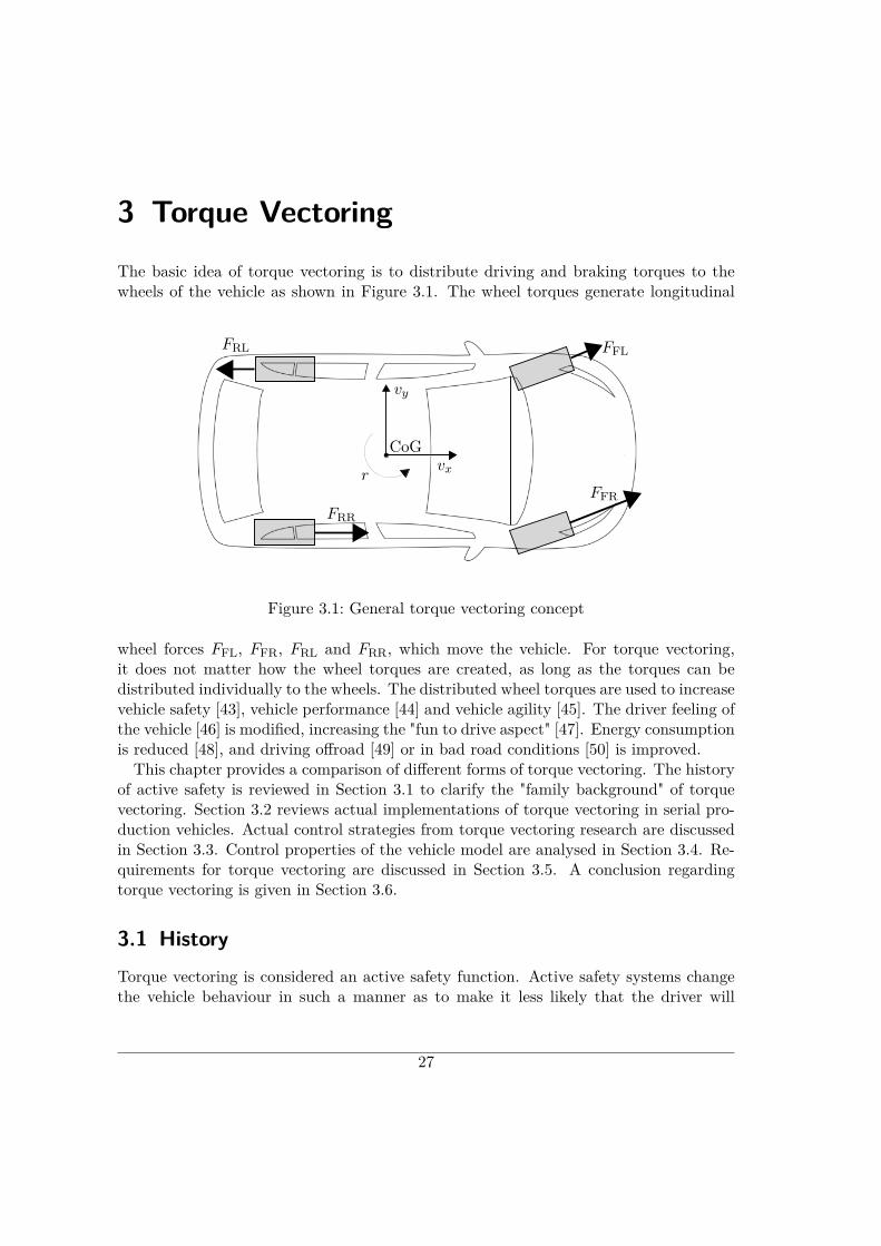
The basic idea of torque vectoring is to distribute driving and braking torques to thewheels of the vehicle as shown in Figure 3.1. The wheel torques generate longitudinal
FFR
FFL
vy
vxr
CoG
FRR
FRL
Figure 3.1: General torque vectoring concept
wheel forces FFL, FFR, FRL and FRR, which move the vehicle. For torque vectoring,it does not matter how the wheel torques are created, as long as the torques can bedistributed individually to the wheels. The distributed wheel torques are used to increasevehicle safety [43], vehicle performance [44] and vehicle agility [45]. The driver feeling ofthe vehicle [46] is modified, increasing the "fun to drive aspect" [47]. Energy consumptionis reduced [48], and driving offroad [49] or in bad road conditions [50] is improved.This chapter provides a comparison of different forms of torque vectoring. The history
of active safety is reviewed in Section 3.1 to clarify the "family background" of torquevectoring. Section 3.2 reviews actual implementations of torque vectoring in serial pro-duction vehicles. Actual control strategies from torque vectoring research are discussedin Section 3.3. Control properties of the vehicle model are analysed in Section 3.4. Re-quirements for torque vectoring are discussed in Section 3.5. A conclusion regardingtorque vectoring is given in Section 3.6.
3.1 HistoryTorque vectoring is considered an active safety function. Active safety systems changethe vehicle behaviour in such a manner as to make it less likely that the driver will
27
28 3 Torque Vectoring
experience an accident. Active safety systems can be divided into two categories. Thefirst category improves the behaviour of the driver: these are described as advanceddriver assistance systems (ADAS). Such systems enhance driver commands and includesystems such as adaptive cruise control (ACC), emergency brake assistant (EBA), nearobject detection system (NODS), lane departure warning (LDW), lane keeping assistancesystem (LKAS) and many more.The second active safety direction improves the behaviour of the vehicle. Such systems
seek to keep the vehicle drivable for as long as possible, considering the vehicle’s physicallimitations. These systems include the anti-lock braking system (ABS), the tractioncontrol system (TCS), electronic stability control (ESC), active roll stabilisation (ARS)and the active suspension system (ASS). ABS, TCS and ESC are briefly reviewed becausetorque vectoring is related to these systems.
3.1.1 Active safety functionsVehicle behaviour is critical for most drivers if the vehicle leaves its linear attitude. Forexample, normal drivers are used to the fact that the vehicle turns more if the steeringwheel is turned more. Now, if the front tyres reach their physical limits for lateralforce generation, more steering does not turn the vehicle more strongly, it may eventurn the vehicle less. This behaviour disturbs the driver and often results in dangerousaccidents [51]. To improve vehicle behaviour in tyre force saturation regimes, severalfunctions have been developed to make the vehicle more manageable for the driver.
ABS
ABS was the first active safety function to have been introduced for serial productionvehicles in the 1970s [35], [51], [52]. ABS solves the problem of locked wheels caused bybraking. If the driver brakes strongly, a high braking pressure is created which resultsin high braking forces acting on the wheels. Excessive braking forces lock the wheels.Locked wheels inhibit lateral wheel forces, so it becomes impossible to turn the vehicle.If the rear wheels are locked, the vehicle turns more, as expected, and even becomesunstable, which results in strong skidding. The ABS monitors the angular velocity ofthe wheels, and if one wheel has a tendency to lock, the brake pressure on the associatedbrake is reduced. With reduced brake pressure, the braking force acting on the wheelis reduced. The tendency of the wheel to lock is decreased, and therefore it becomespossible to generate lateral tyre forces.
TCS
The next active safety function development was TCS [35], [51]. TCS was introducedinto serial production vehicles in the 1980s. ABS solves the problem of locked wheelsduring braking. TCS solves the problem of spinning wheels during acceleration. Thegeneral problem for the driver is the same. If the front wheels are spinning, no lateralforces can be generated and it is impossible to turn the vehicle with the steering wheel.If the rear wheels are spinning, no lateral rear wheel forces are generated and the vehicle
3.2 Vehicles 29
becomes unstable and skids. When TCS recognises a spinning wheel it reduces thepropulsion power of the engine, and, in some versions of TCS, actuates the hydraulicbrakes of the spinning wheel.
ESC
During the 90s ESC [35], [51], [52] was introduced. ABS and TCS deal with tyre forcelimitations for longitudinal requests like braking and accelerating. ESC deals with lateraldrive requests during steering of the vehicle. ESC uses the steering angle of the driverto calculate how much the driver wants to turn the vehicle. The desired turning motionof the vehicle is compared with the actual turning motion. If the vehicle does not turnas much as desired, this is regarded as understeering. For an understeering vehicle, ESCgenerates a braking force on the inner wheel. This braking force generates a yaw momentMz which increases the turning motion of the vehicle. Normally, the inner rear wheelis braked because in an understeering vehicle the front tyre forces are at their frictionlimits. Additional longitudinal forces would also reduce the lateral force capacity, asdiscussed in [53]. The vehicle is considered to be oversteering if it turns more thanexpected. For an oversteering vehicle, braking forces are applied to the outer wheels.Normally, the outer front wheel is braked because in an oversteering vehicle the rearwheels are at their saturation limits. Advanced ESC versions also use the steering angleof the wheels to modify the lateral performance of the vehicle [51].
3.1.2 Interaction of active safety functions
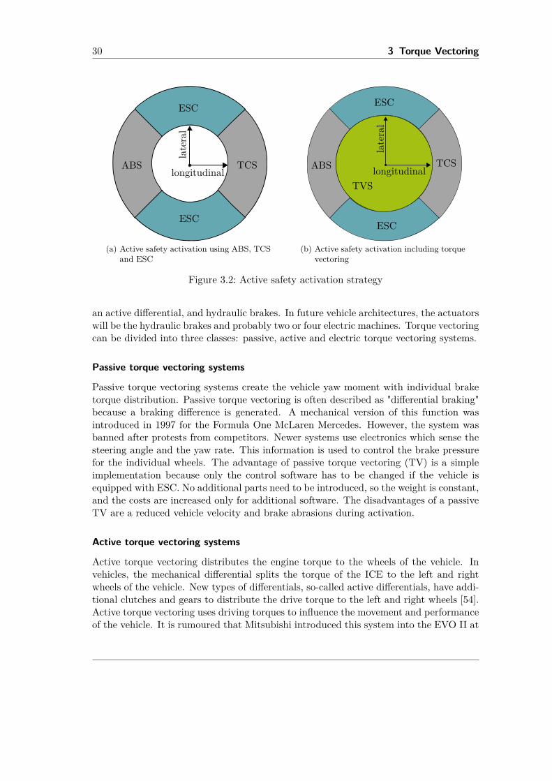
Thus far, individual functions for active safety have been discussed. All of these functionsaim to improve vehicle movement given the physical constraints arising from limitedtyre forces. In most modern vehicles, many functions are included to improve vehiclebehaviour while braking, accelerating and steering. However, each of these functionsis only activated if certain driving limits are exceeded. The maximal tyre forces aredescribed by the friction circle [53]. The active safety functions for improving vehiclebehaviour can be graphically combined with this circle, as shown in Figure 3.2a. Tovisualise the activation strategy of these active safety functions, ABS is active duringstrong braking manoeuvres and ESC is active during strong lateral requests. Torquevectoring can be activated throughout most operation ranges and is not used only insafety critical situations, as indicated in Figure 3.2b. Additionally, ABS, TCS and ESCcan be activated later if torque vectoring is integrated.
3.2 VehiclesTorque vectoring is related to vehicle performance and helps to stabilise the vehicle,which improves driving safety. The key idea of torque vectoring is generating a forcedifference between the left and right wheels for improved cornering performance. Thetorque distribution is performed using the propulsion system and the brakes of thevehicle. In an actual standard vehicle, this is an internal combustion engine, including
30 3 Torque Vectoring
ESC
TCSABS
ESC
longitudinallateral
(a) Active safety activation using ABS, TCSand ESC
ESC
TVS
ABS
ESC
longitudinal
lateral
TCS
(b) Active safety activation including torquevectoring
Figure 3.2: Active safety activation strategy
an active differential, and hydraulic brakes. In future vehicle architectures, the actuatorswill be the hydraulic brakes and probably two or four electric machines. Torque vectoringcan be divided into three classes: passive, active and electric torque vectoring systems.
Passive torque vectoring systems
Passive torque vectoring systems create the vehicle yaw moment with individual braketorque distribution. Passive torque vectoring is often described as "differential braking"because a braking difference is generated. A mechanical version of this function wasintroduced in 1997 for the Formula One McLaren Mercedes. However, the system wasbanned after protests from competitors. Newer systems use electronics which sense thesteering angle and the yaw rate. This information is used to control the brake pressurefor the individual wheels. The advantage of passive torque vectoring (TV) is a simpleimplementation because only the control software has to be changed if the vehicle isequipped with ESC. No additional parts need to be introduced, so the weight is constant,and the costs are increased only for additional software. The disadvantages of a passiveTV are a reduced vehicle velocity and brake abrasions during activation.
Active torque vectoring systems
Active torque vectoring distributes the engine torque to the wheels of the vehicle. Invehicles, the mechanical differential splits the torque of the ICE to the left and rightwheels of the vehicle. New types of differentials, so-called active differentials, have addi-tional clutches and gears to distribute the drive torque to the left and right wheels [54].Active torque vectoring uses driving torques to influence the movement and performanceof the vehicle. It is rumoured that Mitsubishi introduced this system into the EVO II at
3.3 Controller Design 31
the World Rally Championship in 1994. The first serial production vehicle with activetorque vectoring was the Mitsubishi Lancer Evolution IV in 1996. Active systems canbe divided into front-wheel, rear-wheel, and four-wheel based systems. Front- or rear-wheel based, active differentials are easier to build because only one active differentialis required. Three active differentials must be implemented to control four wheels. Thepossibilities for influencing the vehicle behaviour are more intense with four-wheel basedsystems. The advantages of the active TV system are improved agility, the effectivenessof the system, reduced steering effort and no velocity losses. The disadvantage of theactive TV is the introduction of additional parts for the active differential. These com-ponents increase the cost and the weight of the vehicle. Additionally, torque vectoringis only available if the vehicle is accelerating.
Electric torque vectoring systems
Electric torque vectoring systems are suitable for electric vehicles of the 2nd generation.Second generation electric vehicles are equipped with two or four electric machines,driving the wheels independently. These vehicles are considered to contribute an addi-tional torque vectoring class because the electric machines generate positive and negativetorques. High yaw moments can be generated because an electric TV is a combinationof active and passive TV systems. The control of electric machines is fast and accurate,which implies an efficiently controlled vehicle. No active differential is necessary, so noadditional hardware costs or weight are introduced. In the end, no differential is neededat all. As a result, torque vectoring is "for free" in an electric vehicle with two or fourelectric motors.The advantages of fast, strong and accurate yaw moment generation create the draw-
backs of the electric TVS in terms of functional safety [22]. It is important to guaranteethat no undesireable yaw moment is generated that makes the vehicle unstable andrisks serious accidents. Some considerations on this topic are discussed in Section 3.4.However, this problem is considered in detail in [20], [55].A list of serial production vehicles with different torque vectoring systems is given in
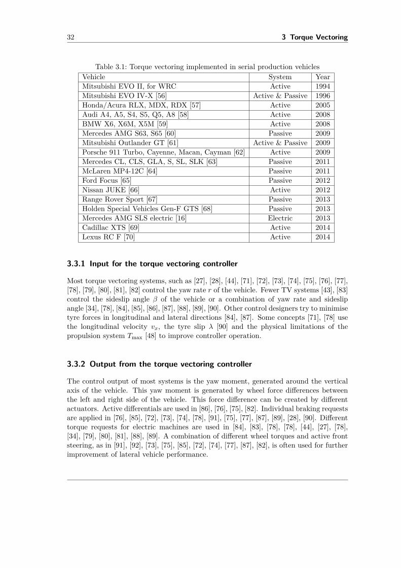
Table 3.1. At present, only one 2nd generation electric vehicle is available as a serialproduct for sale, the Mercedes AMG SLS electric drive [16]. This vehicle is equippedwith four in-chassis electric machines, which drive all four wheels independently.
3.3 Controller Design
Several prototypes have been equipped with torque vectoring algorithms. Different sys-tems have been developed which control the brakes, the propulsion system and thesteering of the wheels. Individual actuation or use a combination of these systems ispossible. Various control strategies are discussed in the literature and frequently-usedconcepts are summarised here. Before analysing the controller algorithm, it is useful toreview the inputs and outputs of different torque vectoring strategies.
32 3 Torque Vectoring
Table 3.1: Torque vectoring implemented in serial production vehiclesVehicle System YearMitsubishi EVO II, for WRC Active 1994Mitsubishi EVO IV-X [56] Active & Passive 1996Honda/Acura RLX, MDX, RDX [57] Active 2005Audi A4, A5, S4, S5, Q5, A8 [58] Active 2008BMW X6, X6M, X5M [59] Active 2008Mercedes AMG S63, S65 [60] Passive 2009Mitsubishi Outlander GT [61] Active & Passive 2009Porsche 911 Turbo, Cayenne, Macan, Cayman [62] Active 2009Mercedes CL, CLS, GLA, S, SL, SLK [63] Passive 2011McLaren MP4-12C [64] Passive 2011Ford Focus [65] Passive 2012Nissan JUKE [66] Active 2012Range Rover Sport [67] Passive 2013Holden Special Vehicles Gen-F GTS [68] Passive 2013Mercedes AMG SLS electric [16] Electric 2013Cadillac XTS [69] Active 2014Lexus RC F [70] Active 2014
3.3.1 Input for the torque vectoring controller
Most torque vectoring systems, such as [27], [28], [44], [71], [72], [73], [74], [75], [76], [77],[78], [79], [80], [81], [82] control the yaw rate r of the vehicle. Fewer TV systems [43], [83]control the sideslip angle β of the vehicle or a combination of yaw rate and sideslipangle [34], [78], [84], [85], [86], [87], [88], [89], [90]. Other control designers try to minimisetyre forces in longitudinal and lateral directions [84], [87]. Some concepts [71], [78] usethe longitudinal velocity vx, the tyre slip λ [90] and the physical limitations of thepropulsion system Tmax [48] to improve controller operation.
3.3.2 Output from the torque vectoring controller
The control output of most systems is the yaw moment, generated around the verticalaxis of the vehicle. This yaw moment is generated by wheel force differences betweenthe left and right side of the vehicle. This force difference can be created by differentactuators. Active differentials are used in [86], [76], [75], [82]. Individual braking requestsare applied in [76], [85], [72], [73], [74], [78], [91], [75], [77], [87], [89], [28], [90]. Differenttorque requests for electric machines are used in [84], [83], [78], [78], [44], [27], [78],[34], [79], [80], [81], [88], [89]. A combination of different wheel torques and active frontsteering, as in [91], [92], [73], [75], [85], [72], [74], [77], [87], [82], is often used for furtherimprovement of lateral vehicle performance.
3.3 Controller Design 33
3.3.3 Control lawsDifferent control laws are used for torque vectoring. Frequently-used control strategiesare briefly discussed here.
Feed forward control
The torque distribution between the left and right sides can be operated in an open-loop scheme. The steering angle δ is the input for the controller, and the output of thecontroller is the desired yaw moment Mz. The desired yaw moment is often describedas
Mz = g(vx)δ, (3.1)
where the nonlinear function g depends on longitudinal velocity vx. Several concepts forthe function g(vx) are available.• The function g(vx) is a parameter-dependent gain [84], [93], [94]. This mapping isinfluenced by vehicle parameters and the longitudinal velocity.
• The dynamic behaviour is further improved if an additional time constant is in-cluded in the parameter-dependent gain [93].
• A look-up table is used for the mapping from the steering angle to the yaw moment[48], [34]. Additional limitations are introduced into the look-up table to cope withmotor saturations and lateral boundaries.
• A flatness based feed-forward controller is used in [88] to improve the dynamicbehaviour of the controller during dynamic vehicle manoeuvres.
• The dynamic model inversion technique, as in [91], is similar to the flatness basedfeed-forward controller and this technique is also used to improve the dynamicbehaviour of the vehicle.
The advantages of feed-forward solutions are low computation effort and simple im-plementation of the controller, with accurate and fast performance for an appropriatemodel. The drawback of feed-forward solutions is sensitivity to noise and model vari-ance. A feed-forward controller improves the performance of the closed-loop system butit is beneficial to include a feedback controller for parameter variations. In combinedsolutions, the feed-forward controller is used to improve the performance of the closed-loop, and the feedback controller is introduced to deal with varying system parametersor disturbances.
PID control
The proportional-integral-derivative (PID) controller is the classic control structure andthe most commonly used controller in practical applications [95]. The PID controller iswell known, straightforward to implement, and detailed tuning rules are available [95].Torque vectoring is designed with PID-controllers in [92], [78], [43], [80], [81], [96].
34 3 Torque Vectoring
Sliding mode control
Sliding mode control is a non-linear control technique that forces the system to slidealong a defined surface. Sliding mode control is appropriate for automotive applicationsbecause of its robustness and low computation effort. Different sliding mode controlconcepts are proposed for torque vectoring in [27], [75], [78], [86], [90], [92], [97].
Predictive control
Some authors propose interesting results with model predictive control algorithms [33],[74], [87], [98], [99]. In model predictive control, the controller estimates the futurebehaviour of the system from specific inputs and minimises a given performance indexto find the best control input.
Fuzzy control
Fuzzy control is widely used in control applications where human operators control thesystem with a set of rules for several inputs. Torque vectoring is not a typical applicationfor fuzzy control, but [28] and [85] showed interesting results.
Optimal and robust control
Advanced linear control design methods from optimal and robust control are also appliedto torque vectoring. For example, [34], [88], [90], [100], [89] use linear-quadratic-Gaussian(LQG) controllers. H∞ controllers are used by [101], [102].
LPV control
An extension of optimal and robust control techniques is LPV control. The ideas of H∞and H2 control are extended from linear time-invariant (LTI) systems to a certain classof non-linear systems.
• Interesting results are obtained by [77], [73], [103] where scheduling signals areused to choose between active front steering and brake force distribution.
• The major non-linearities in vehicle dynamics are related to non-linear tyre forces,described in Section 2.2.1. Baslamish [104] and Baslamish et al. [72] used tyrestates like tyre slip λ and tyre slip angle α as scheduling parameters.
• The surface condition of the road has a major effect on tyre force generation.Therefore Fallah et al. [50] used the maximal adhesion coefficient of the road µ asa scheduling parameter.
• Palladino et al. [71], [105], Liu et al. [79], Kaiser et al. [106], [107] and Bartels etal. [108] define scheduling signals related to the longitudinal velocity of the vehicle.These approaches govern the non-linear behaviour of the single-track vehicle model.
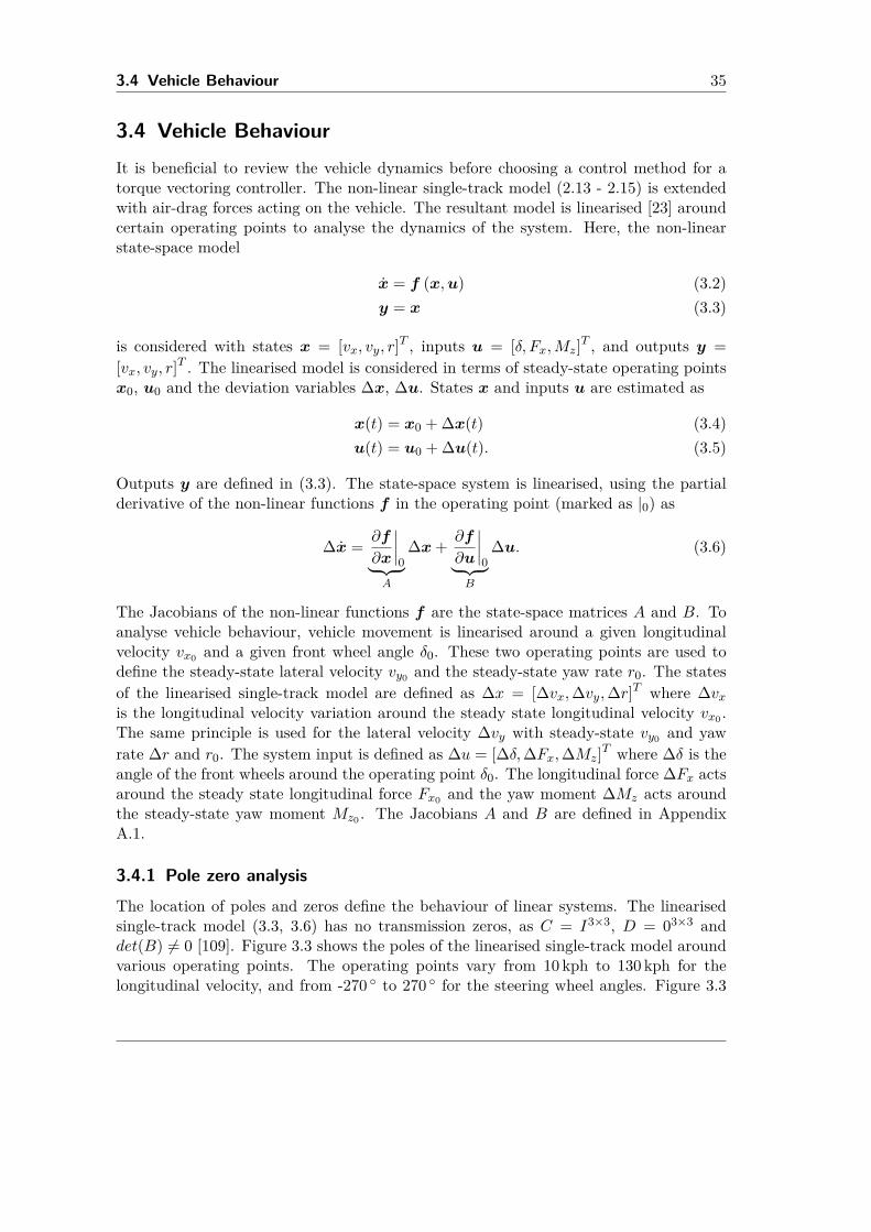
3.4 Vehicle Behaviour 35
3.4 Vehicle BehaviourIt is beneficial to review the vehicle dynamics before choosing a control method for atorque vectoring controller. The non-linear single-track model (2.13 - 2.15) is extendedwith air-drag forces acting on the vehicle. The resultant model is linearised [23] aroundcertain operating points to analyse the dynamics of the system. Here, the non-linearstate-space model
x = f (x,u) (3.2)y = x (3.3)
is considered with states x = [vx, vy, r]T , inputs u = [δ, Fx,Mz]T , and outputs y =[vx, vy, r]T . The linearised model is considered in terms of steady-state operating pointsx0, u0 and the deviation variables ∆x, ∆u. States x and inputs u are estimated as
x(t) = x0 + ∆x(t) (3.4)u(t) = u0 + ∆u(t). (3.5)
Outputs y are defined in (3.3). The state-space system is linearised, using the partialderivative of the non-linear functions f in the operating point (marked as |0) as
∆x = ∂f
∂x
∣∣∣∣0︸ ︷︷ ︸
A
∆x+ ∂f
∂u
∣∣∣∣0︸ ︷︷ ︸
B
∆u. (3.6)
The Jacobians of the non-linear functions f are the state-space matrices A and B. Toanalyse vehicle behaviour, vehicle movement is linearised around a given longitudinalvelocity vx0 and a given front wheel angle δ0. These two operating points are used todefine the steady-state lateral velocity vy0 and the steady-state yaw rate r0. The statesof the linearised single-track model are defined as ∆x = [∆vx,∆vy,∆r]T where ∆vxis the longitudinal velocity variation around the steady state longitudinal velocity vx0 .The same principle is used for the lateral velocity ∆vy with steady-state vy0 and yawrate ∆r and r0. The system input is defined as ∆u = [∆δ,∆Fx,∆Mz]T where ∆δ is theangle of the front wheels around the operating point δ0. The longitudinal force ∆Fx actsaround the steady state longitudinal force Fx0 and the yaw moment ∆Mz acts aroundthe steady-state yaw moment Mz0 . The Jacobians A and B are defined in AppendixA.1.
3.4.1 Pole zero analysisThe location of poles and zeros define the behaviour of linear systems. The linearisedsingle-track model (3.3, 3.6) has no transmission zeros, as C = I3×3, D = 03×3 anddet(B) 6= 0 [109]. Figure 3.3 shows the poles of the linearised single-track model aroundvarious operating points. The operating points vary from 10 kph to 130 kph for thelongitudinal velocity, and from -270 to 270 for the steering wheel angles. Figure 3.3
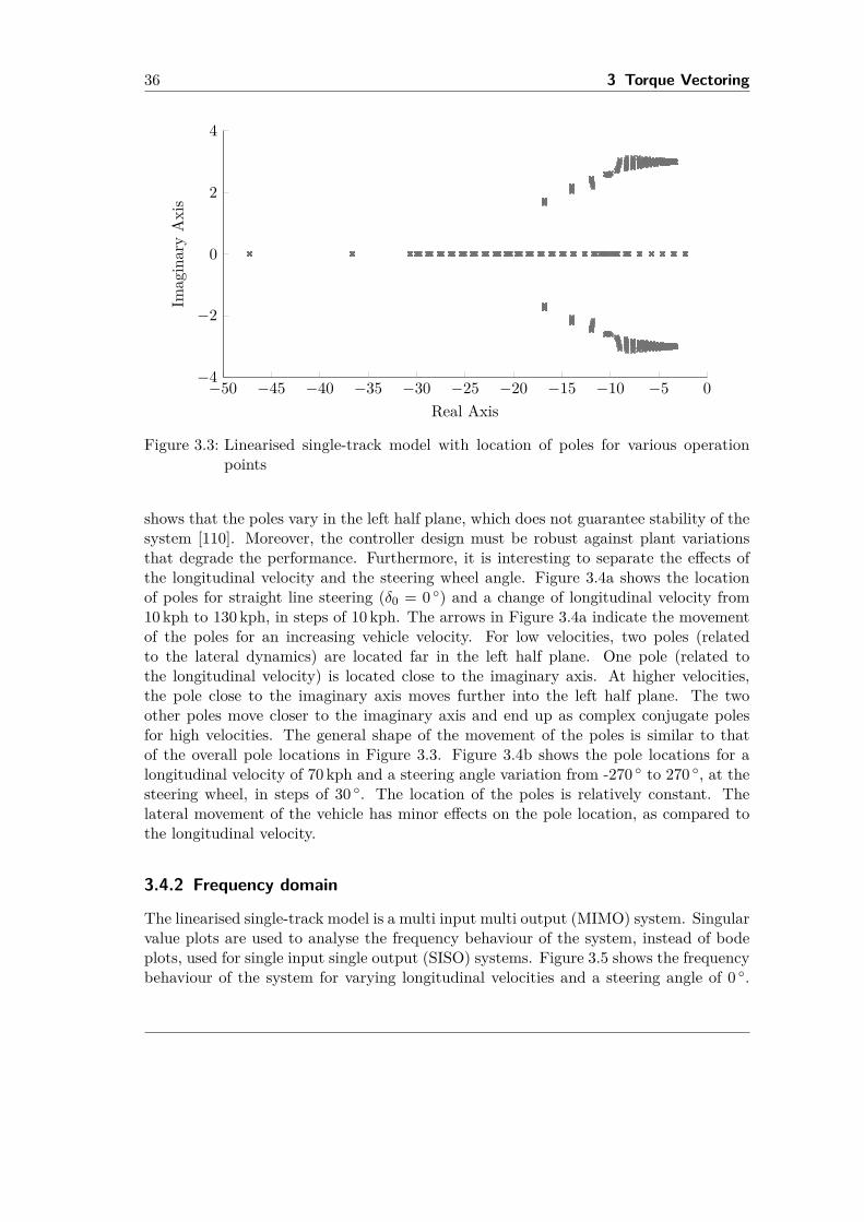
36 3 Torque Vectoring
−50 −45 −40 −35 −30 −25 −20 −15 −10 −5 0−4
−2
0
2
4
Real Axis
Imag
inar
yA
xis
Figure 3.3: Linearised single-track model with location of poles for various operationpoints
shows that the poles vary in the left half plane, which does not guarantee stability of thesystem [110]. Moreover, the controller design must be robust against plant variationsthat degrade the performance. Furthermore, it is interesting to separate the effects ofthe longitudinal velocity and the steering wheel angle. Figure 3.4a shows the locationof poles for straight line steering (δ0 = 0 ) and a change of longitudinal velocity from10 kph to 130 kph, in steps of 10 kph. The arrows in Figure 3.4a indicate the movementof the poles for an increasing vehicle velocity. For low velocities, two poles (relatedto the lateral dynamics) are located far in the left half plane. One pole (related tothe longitudinal velocity) is located close to the imaginary axis. At higher velocities,the pole close to the imaginary axis moves further into the left half plane. The twoother poles move closer to the imaginary axis and end up as complex conjugate polesfor high velocities. The general shape of the movement of the poles is similar to thatof the overall pole locations in Figure 3.3. Figure 3.4b shows the pole locations for alongitudinal velocity of 70 kph and a steering angle variation from -270 to 270 , at thesteering wheel, in steps of 30 . The location of the poles is relatively constant. Thelateral movement of the vehicle has minor effects on the pole location, as compared tothe longitudinal velocity.
3.4.2 Frequency domain
The linearised single-track model is a multi input multi output (MIMO) system. Singularvalue plots are used to analyse the frequency behaviour of the system, instead of bodeplots, used for single input single output (SISO) systems. Figure 3.5 shows the frequencybehaviour of the system for varying longitudinal velocities and a steering angle of 0 .
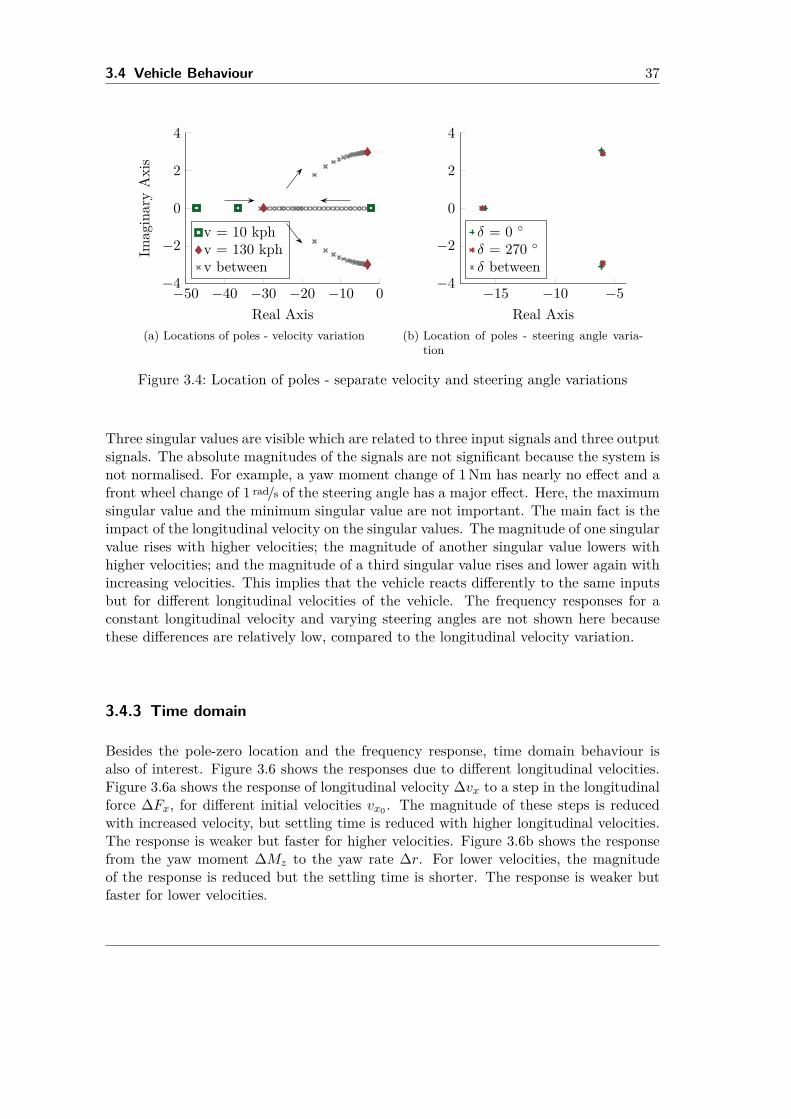
3.4 Vehicle Behaviour 37
−50 −40 −30 −20 −10 0−4
−2
0
2
4
Real Axis
Imag
inar
yA
xis
v = 10 kphv = 130 kphv between
(a) Locations of poles - velocity variation
−15 −10 −5−4
−2
0
2
4
Real Axis
δ = 0
δ = 270
δ between
(b) Location of poles - steering angle varia-tion
Figure 3.4: Location of poles - separate velocity and steering angle variations
Three singular values are visible which are related to three input signals and three outputsignals. The absolute magnitudes of the signals are not significant because the system isnot normalised. For example, a yaw moment change of 1Nm has nearly no effect and afront wheel change of 1 rad/s of the steering angle has a major effect. Here, the maximumsingular value and the minimum singular value are not important. The main fact is theimpact of the longitudinal velocity on the singular values. The magnitude of one singularvalue rises with higher velocities; the magnitude of another singular value lowers withhigher velocities; and the magnitude of a third singular value rises and lower again withincreasing velocities. This implies that the vehicle reacts differently to the same inputsbut for different longitudinal velocities of the vehicle. The frequency responses for aconstant longitudinal velocity and varying steering angles are not shown here becausethese differences are relatively low, compared to the longitudinal velocity variation.
3.4.3 Time domain
Besides the pole-zero location and the frequency response, time domain behaviour isalso of interest. Figure 3.6 shows the responses due to different longitudinal velocities.Figure 3.6a shows the response of longitudinal velocity ∆vx to a step in the longitudinalforce ∆Fx, for different initial velocities vx0 . The magnitude of these steps is reducedwith increased velocity, but settling time is reduced with higher longitudinal velocities.The response is weaker but faster for higher velocities. Figure 3.6b shows the responsefrom the yaw moment ∆Mz to the yaw rate ∆r. For lower velocities, the magnitudeof the response is reduced but the settling time is shorter. The response is weaker butfaster for lower velocities.
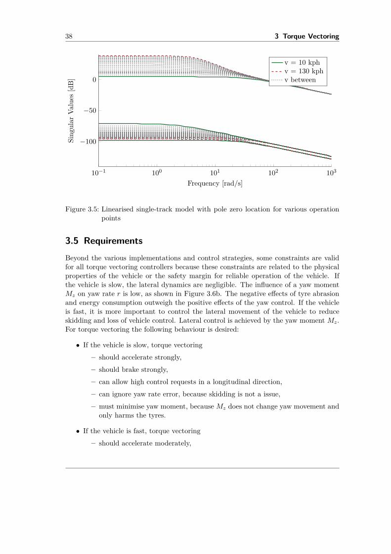
38 3 Torque Vectoring
10−1 100 101 102 103
−100
−50
0
Frequency [rad/s]
Sing
ular
Valu
es[d
B]v = 10 kphv = 130 kphv between
Figure 3.5: Linearised single-track model with pole zero location for various operationpoints
3.5 Requirements
Beyond the various implementations and control strategies, some constraints are validfor all torque vectoring controllers because these constraints are related to the physicalproperties of the vehicle or the safety margin for reliable operation of the vehicle. Ifthe vehicle is slow, the lateral dynamics are negligible. The influence of a yaw momentMz on yaw rate r is low, as shown in Figure 3.6b. The negative effects of tyre abrasionand energy consumption outweigh the positive effects of the yaw control. If the vehicleis fast, it is more important to control the lateral movement of the vehicle to reduceskidding and loss of vehicle control. Lateral control is achieved by the yaw moment Mz.For torque vectoring the following behaviour is desired:
• If the vehicle is slow, torque vectoring– should accelerate strongly,– should brake strongly,– can allow high control requests in a longitudinal direction,– can ignore yaw rate error, because skidding is not a issue,– must minimise yaw moment, becauseMz does not change yaw movement and
only harms the tyres.
• If the vehicle is fast, torque vectoring– should accelerate moderately,
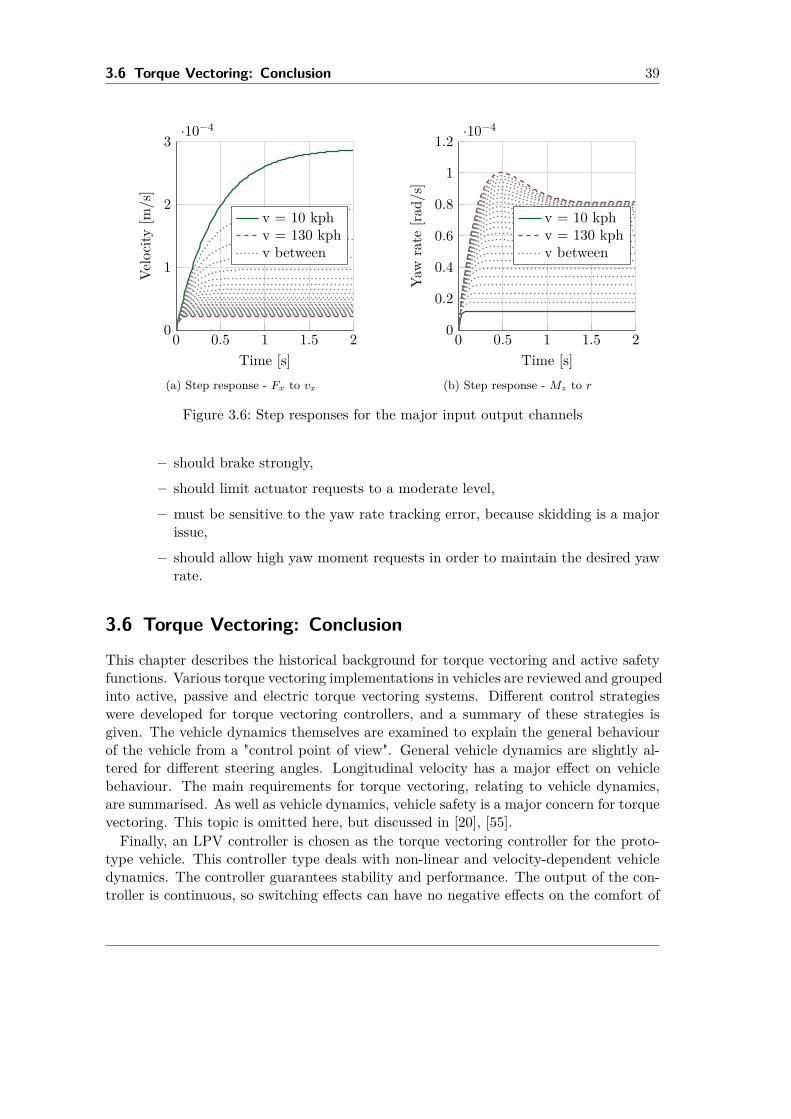
3.6 Torque Vectoring: Conclusion 39
0 0.5 1 1.5 20
1
2
3·10−4
Time [s]
Velo
city
[m/s
]
v = 10 kphv = 130 kphv between
(a) Step response - Fx to vx
0 0.5 1 1.5 20
0.2
0.4
0.6
0.8
1
1.2·10−4
Time [s]
Yaw
rate
[rad/
s]
v = 10 kphv = 130 kphv between
(b) Step response - Mz to r
Figure 3.6: Step responses for the major input output channels
– should brake strongly,– should limit actuator requests to a moderate level,– must be sensitive to the yaw rate tracking error, because skidding is a major
issue,– should allow high yaw moment requests in order to maintain the desired yaw
rate.
3.6 Torque Vectoring: Conclusion
This chapter describes the historical background for torque vectoring and active safetyfunctions. Various torque vectoring implementations in vehicles are reviewed and groupedinto active, passive and electric torque vectoring systems. Different control strategieswere developed for torque vectoring controllers, and a summary of these strategies isgiven. The vehicle dynamics themselves are examined to explain the general behaviourof the vehicle from a "control point of view". General vehicle dynamics are slightly al-tered for different steering angles. Longitudinal velocity has a major effect on vehiclebehaviour. The main requirements for torque vectoring, relating to vehicle dynamics,are summarised. As well as vehicle dynamics, vehicle safety is a major concern for torquevectoring. This topic is omitted here, but discussed in [20], [55].Finally, an LPV controller is chosen as the torque vectoring controller for the proto-
type vehicle. This controller type deals with non-linear and velocity-dependent vehicledynamics. The controller guarantees stability and performance. The output of the con-troller is continuous, so switching effects can have no negative effects on the comfort of
40 3 Torque Vectoring
the ride. The tuning of the controller is systematic and saves development time. Thereal-time implementation of an LPV controller on an automotive microcontroller shouldbe possible if this point is taken into consideration during the design of the controller.
4 LPV Modelling and Control of theVehicle
As seen in Chapter 2, the vehicle model for torque vectoring is non-linear and parameter-dependent. Non-linear control theory offers ways to design controllers, but these tendto be complex in synthesis and implementation, and are often difficult to tune for goodperformance. For this reason, in practice linear control techniques are often used evenfor non-linear systems, from simple proportional (P) controllers, to PID controllers tolinear-quadratic regulator (LQR) and LQG or more advanced H∞ or H2 controllers. Toapply linear control techniques to non-linear plants, several strategies are possible:
• The controller is designed to be robust. The non-linear characteristics are treatedas time-varying uncertainties. The controller copes with variations and achievesa stable closed-loop system. This approach sometimes leads to unsatisfactoryperformance because one controller has to handle all non-linear characteristics.The controller has to guarantee stability for a wide range of parameter variations,which normally reduces the performance of the closed-loop system.
• Another possibility is linearising the non-linear model at certain points in the op-eration range and calculating appropriate controllers for these points. A switchingsequence, interpolation scheme or lookup table is used to control the non-linearsystem between its defined linearisation points. This method is called (heuristic)gain-scheduling control and is often used in practical applications. Gain-scheduledcontrollers benefit from a simple application, good performance and low compu-tation effort. A drawback of gain-scheduled control is the cumbersome searchfor linearisation points. The design of the scheduling process is tedious as it re-quires time to find an acceptable switching strategy. The most serious drawback ofgain-scheduling control is the loss of stability and performance guarantees for thecontroller design. In practice, many simulations are performed to ensure stability,but the danger of losing stability in an unfortunate switching sequence remains aconcern.
• A way of extending well-tried linear techniques, such as H∞ control, to non-linearsystems is to use LPV gain scheduling. Conditions for stability and performanceof the closed-loop systems are expressed as convex optimisation problems. Theconvex optimisation problem is defined as linear matrix inequality (LMI). SeveralLMIs can be combined for more tuning requirements, and the LMIs are solved withnumerical tools like [111], [112]. The advantage of linear parameter-varying controldesign is that LPV guarantees stability and performance of the closed-loop system.
41
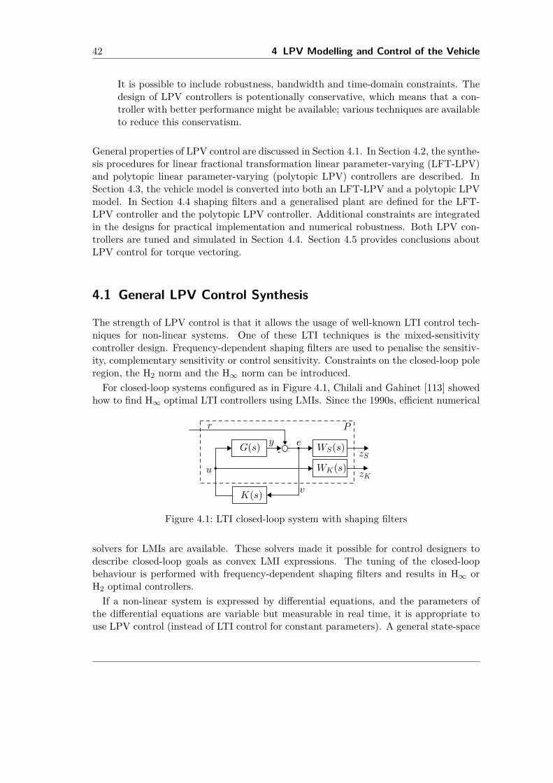
42 4 LPV Modelling and Control of the Vehicle
It is possible to include robustness, bandwidth and time-domain constraints. Thedesign of LPV controllers is potentionally conservative, which means that a con-troller with better performance might be available; various techniques are availableto reduce this conservatism.
General properties of LPV control are discussed in Section 4.1. In Section 4.2, the synthe-sis procedures for linear fractional transformation linear parameter-varying (LFT-LPV)and polytopic linear parameter-varying (polytopic LPV) controllers are described. InSection 4.3, the vehicle model is converted into both an LFT-LPV and a polytopic LPVmodel. In Section 4.4 shaping filters and a generalised plant are defined for the LFT-LPV controller and the polytopic LPV controller. Additional constraints are integratedin the designs for practical implementation and numerical robustness. Both LPV con-trollers are tuned and simulated in Section 4.4. Section 4.5 provides conclusions aboutLPV control for torque vectoring.
4.1 General LPV Control Synthesis
The strength of LPV control is that it allows the usage of well-known LTI control tech-niques for non-linear systems. One of these LTI techniques is the mixed-sensitivitycontroller design. Frequency-dependent shaping filters are used to penalise the sensitiv-ity, complementary sensitivity or control sensitivity. Constraints on the closed-loop poleregion, the H2 norm and the H∞ norm can be introduced.For closed-loop systems configured as in Figure 4.1, Chilali and Gahinet [113] showed
how to find H∞ optimal LTI controllers using LMIs. Since the 1990s, efficient numerical
K(s)
G(s) y
u
r
zS
eWS(s)
WK(s)zK
-
P
v
Figure 4.1: LTI closed-loop system with shaping filters
solvers for LMIs are available. These solvers made it possible for control designers todescribe closed-loop goals as convex LMI expressions. The tuning of the closed-loopbehaviour is performed with frequency-dependent shaping filters and results in H∞ orH2 optimal controllers.If a non-linear system is expressed by differential equations, and the parameters of
the differential equations are variable but measurable in real time, it is appropriate touse LPV control (instead of LTI control for constant parameters). A general state-space
4.1 General LPV Control Synthesis 43
description [114], [115] of an LPV system G(ρ)
G(ρ) :x = A(ρ)x+B(ρ)wz = C(ρ)x+D(ρ)w (4.1)
shows the close relation to LTI state-space models. The signals x, x, w, z, and ρ dependon the time t which is not shown here for an simplified expression. The state vectoris defined as x ∈ Rn, the input vector as w ∈ Rm and the output vector as z ∈ Rl.For LPV systems, the state-space matrices A(ρ), B(ρ), C(ρ) and D(ρ) are continuousfunctions of ρ ∈ Rp and describe the varying behaviour of the model. The schedulingparameters ρ are directly measurable. However, ρ is assumed to be restricted to theadmissible scheduling parameter set
P ⊂ Rp : ρ ∈ P,∀t > 0, (4.2)
which is assumed to be compact. The scheduling signals ρ are often considered asexternal signals, which means that the system is linear in input and states. Non-linearsystems can be represented by allowing the model matrices of an LPV system to dependon state variables, inputs or outputs. In this case the model is referred to as quasi-LPVsystem. Quasi-LPV systems are more difficult to analyse because the bounds of thescheduling parameters cannot be limited a priori.Closed-loop stability is established by Lyapunov stability [116], [114], [117]. Perfor-
mance of the closed-loop system is expressed by the induced L2-norm [118]. In [118],the L2-gain is defined as follows:Definition 4.1 Let γ ≥ 0. The system is said to have L2 less than or equal to γ if∫ T
0‖z(t)‖2 dt ≤ γ2
∫ T
0‖w(t)‖2 dt (4.3)
for all T ≥ 0 and all w ∈ L2(0, T ), with ... initial state x(0) = x0.The induced L2-norm of a system expresses the maximum amplification from the inputw(t) to the output z(t) in terms of the L2 signal norm.Typical fields for LPV controller applications are aerospace [119], [120], [121], [122],
robotics [123], [124], [125] and automotive engineering [126], [127], [128]. In practise,there are three major approaches to LPV control of non-linear plants. These approachesare gridding-based linear parameter-varying (gridding-based LPV) control, LFT-LPVcontrol and polytopic LPV control.
4.1.1 Polytopic LPV control
The polytopic LPV design [114], [129] is an extreme form of gridding-based LPV control,where only gridding points at the vertices of a convex polytope P that covers the admis-sible parameter range are checked. Checking only the vertices is possible if the modeldepends affinely on the parameters. For polytopic LPV control, a quadratic Lyapunovfunction is used, which guarantees stability across all vertex coordinates. In the synthe-
44 4 LPV Modelling and Control of the Vehicle
sis process, a stable controller is searched for every vertex point of the convex hull andthe resulting controllers are linearly interpolated to control the entire parameter range.An LPV model
x = A(θ)x+B(θ)wz = C(θ)x+D(θ)w,
(4.4)
where θ(t) ∈ P, ∀t ≥ 0 for a given compact set P ⊂ Rnθ is polytopic if it satisfies thefollowing two conditions.
1. The set P is a polytope, i.e. it can be expressed as a convex hull
P = Co θv1, θv2, ..., θvr , (4.5)
where the θvi ∈ Rnθ are the vertices of the polytope and r is the number of vertices.The representation (4.5) implies that
P =θ ∈ Rnθ |θ =
r∑i=1
αiθvi,r∑i=1
αi = 1, αi ≥ 0, i = 1, ..., r. (4.6)
The coefficients αi are referred to as convex coordinates.
2. The model (4.4) depends affinely on the parameter vector θ. In this case, the setof admissible LTI systems can be represented by[
A(θ) B(θ)C(θ) D(θ)
]=Co
[A(θ) B(θ)C(θ) D(θ)
], i = 1, ..., r
∀θ ∈ P, (4.7)
where
(Ai, Bi, Ci, Di) = (A(θvi), B(θvi), C(θvi), D(θvi)) , i = 1, ..., r (4.8)
are the vertex plants. More generally, if
θ(t) =r∑i=1
αiθvi, (4.9)
then [A(θ) B(θ)C(θ) D(θ)
]=
r∑i=1
αi
[Ai BiCi Di
], (4.10)
where the αi are convex coordinates.
Minimum values θi and maximum values θi limit the scheduling parameters to definethe polytope. Not every trajectory in P may be physically possible, which introducesconservatism into the design [130]. A mathematical representation of the polytopic LPV
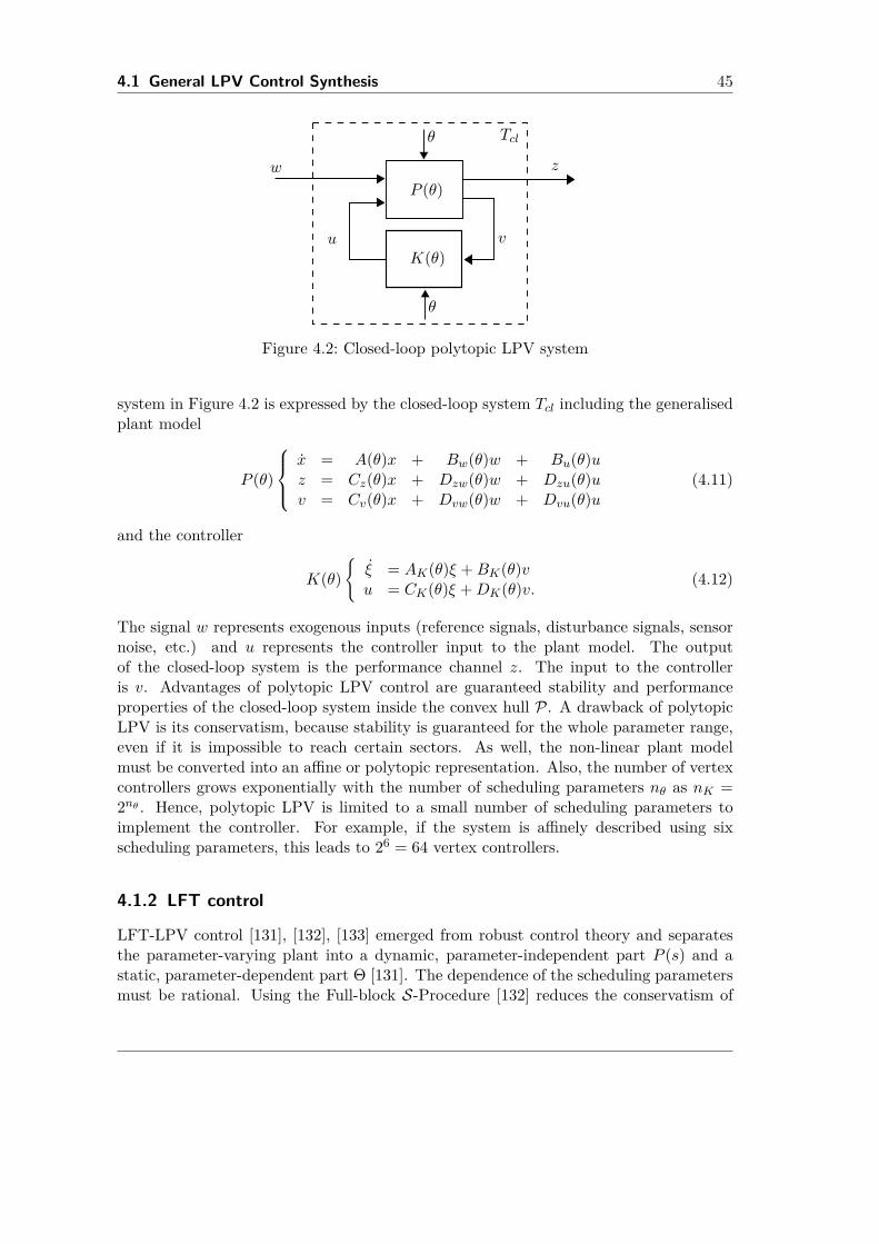
4.1 General LPV Control Synthesis 45
K(θ)
P (θ)
vu
w z
Tclθ
θ
Figure 4.2: Closed-loop polytopic LPV system
system in Figure 4.2 is expressed by the closed-loop system Tcl including the generalisedplant model
P (θ)
x = A(θ)x + Bw(θ)w + Bu(θ)uz = Cz(θ)x + Dzw(θ)w + Dzu(θ)uv = Cv(θ)x + Dvw(θ)w + Dvu(θ)u
(4.11)
and the controller
K(θ)ξ = AK(θ)ξ +BK(θ)vu = CK(θ)ξ +DK(θ)v. (4.12)
The signal w represents exogenous inputs (reference signals, disturbance signals, sensornoise, etc.) and u represents the controller input to the plant model. The outputof the closed-loop system is the performance channel z. The input to the controlleris v. Advantages of polytopic LPV control are guaranteed stability and performanceproperties of the closed-loop system inside the convex hull P. A drawback of polytopicLPV is its conservatism, because stability is guaranteed for the whole parameter range,even if it is impossible to reach certain sectors. As well, the non-linear plant modelmust be converted into an affine or polytopic representation. Also, the number of vertexcontrollers grows exponentially with the number of scheduling parameters nθ as nK =2nθ . Hence, polytopic LPV is limited to a small number of scheduling parameters toimplement the controller. For example, if the system is affinely described using sixscheduling parameters, this leads to 26 = 64 vertex controllers.
4.1.2 LFT control
LFT-LPV control [131], [132], [133] emerged from robust control theory and separatesthe parameter-varying plant into a dynamic, parameter-independent part P (s) and astatic, parameter-dependent part Θ [131]. The dependence of the scheduling parametersmust be rational. Using the Full-block S-Procedure [132] reduces the conservatism of
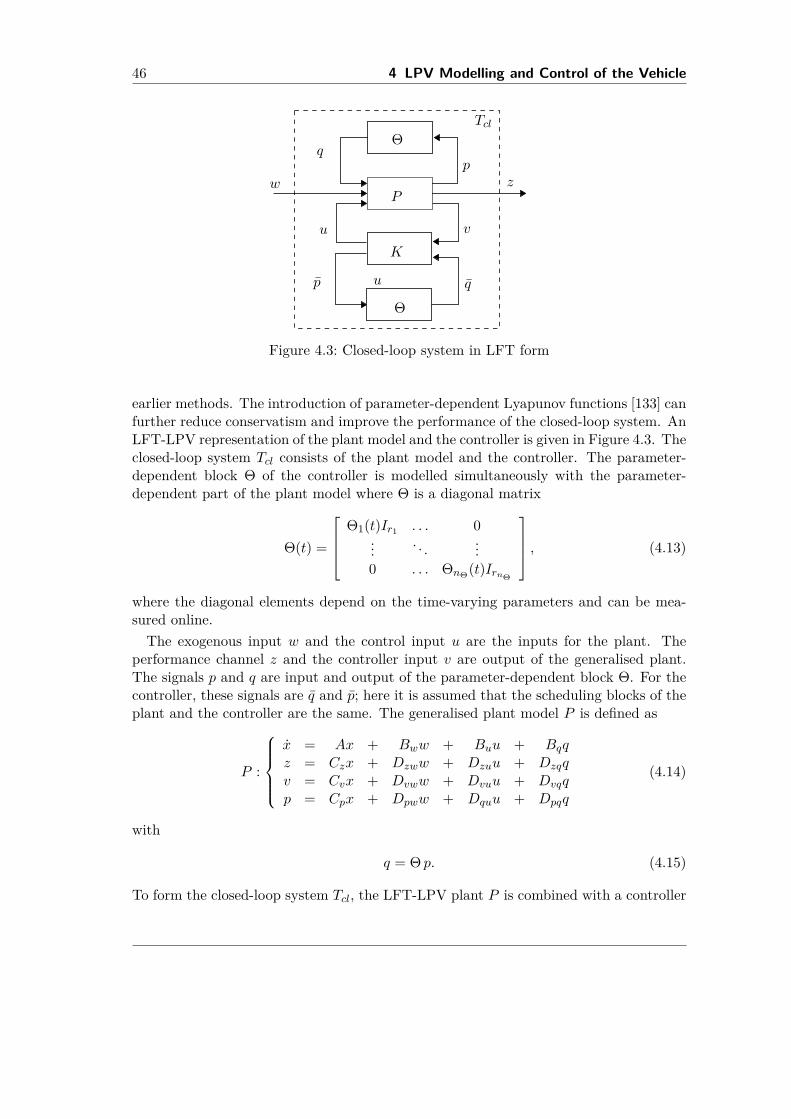
46 4 LPV Modelling and Control of the Vehicle
Θ
K
P
p
vu
q
w z
Tcl
up q
Θ
Figure 4.3: Closed-loop system in LFT form
earlier methods. The introduction of parameter-dependent Lyapunov functions [133] canfurther reduce conservatism and improve the performance of the closed-loop system. AnLFT-LPV representation of the plant model and the controller is given in Figure 4.3. Theclosed-loop system Tcl consists of the plant model and the controller. The parameter-dependent block Θ of the controller is modelled simultaneously with the parameter-dependent part of the plant model where Θ is a diagonal matrix
Θ(t) =
Θ1(t)Ir1 . . . 0
... . . . ...0 . . . ΘnΘ(t)IrnΘ
, (4.13)
where the diagonal elements depend on the time-varying parameters and can be mea-sured online.The exogenous input w and the control input u are the inputs for the plant. The
performance channel z and the controller input v are output of the generalised plant.The signals p and q are input and output of the parameter-dependent block Θ. For thecontroller, these signals are q and p; here it is assumed that the scheduling blocks of theplant and the controller are the same. The generalised plant model P is defined as
P :
x = Ax + Bww + Buu + Bqqz = Czx + Dzww + Dzuu + Dzqqv = Cvx + Dvww + Dvuu + Dvqqp = Cpx + Dpww + Dquu + Dpqq
(4.14)
with
q = Θ p. (4.15)
To form the closed-loop system Tcl, the LFT-LPV plant P is combined with a controller
4.2 LPV Controller Synthesis 47
K. The interconnection is shown in Figure 4.3 and the controller is defined as
K :
ξ = AKξ + BKvv + BKq qu = CKuξ + DKuvv + DKuq qp = CKpξ + DKpvv + DKpq q
(4.16)
with
q = Θ p. (4.17)
The states of the controller are defined as ξ. The controller inputs are v from thegeneralised plant and q for the uncertainty. The outputs are the control input u andthe uncertainty input p. The linear fractional transformation approach [132], [133] ap-plies H∞ design methods for a wide range of parameter varying systems. The use ofparameter-dependent Lyapunov functions reduces the conservatism of the design and isrecommended by [133].For the application considered here, the polytopic LPV controller design and the
LFT-LPV controller design appear to be promising. In the next section, both synthesisprocedures are reviewed and then the polytopic LPV and the LFT-LPV torque vectoringcontrollers are compared.
4.2 LPV Controller Synthesis
For the LPV controller synthesis, two different approaches are summarised. First, thedesign method of Wu and Dong [133] is shown for an LFT-LPV controller with theFull-block S-Procedure and a quadratic, parameter-dependent Lyapunov function. Theconservatism of this design is reduced, as compared with previous designs, such as [131],[132]. Next, the design of a polytopic LPV controller [129], [114] is shown. Beforecalculating the controller, the generalised plant is normalised as described in [23]. Themodification of the plant signals improves the numerical condition of the LMI solvers[111], and it is an important step for a numerically successful controller calculation.
4.2.1 LFT - controller synthesis
To obtain the LFT controller (4.16, 4.17), Wu [133] proposes the following procedure:
1. The generalised plant (4.14, 4.15) must be converted into a generalised plant thatabsorbs the parameter-dependent components as
P (Θ) :
x = A(Θ)x + Bw(Θ)w + Bu(Θ)uz = Cz(Θ)x + Dzw(Θ)w + Dzu(Θ)uv = Cv(Θ)x + Dvw(Θ)w + Dvu(Θ)u
(4.18)
48 4 LPV Modelling and Control of the Vehicle
using A(Θ) Bw(Θ) Bu(Θ)Cz(Θ) Dzw(Θ) Dzu(Θ)Cv(Θ) Dvw(Θ) Dvu(Θ)
=
A Bw BuCz Dzw Dzu
Cv Dvw Dvu
+
BqDzq
Dvq
Θ (I −DpqΘ)−1
CqDqw
Dqu
T
.
(4.19)
The new system is used for controller synthesis. Additionally, the following as-sumptions are introduced by Wu:
• The triple (A(Θ), Bu(Θ), Cv(Θ)) is parameter-dependent, stabilisable anddetectable for all Θ ∈ P.
• The matrices [Cv(Θ),Dvw(Θ)] and [BTu (Θ),DTzu(Θ)] have full row rank for allΘ.
• The matrices Dzw(Θ) = 0 and Dvu(Θ) = 0.
2. For the synthesis, quadratic, parameter-dependent Lyapunov functions R(Θ) andS(Θ) need to be constructed. These matrices are defined as
R(Θ) = T TR (Θ)P TR(Θ) (4.20)S(Θ) = T TS (Θ)QTS(Θ). (4.21)
The parametrization factors TR(Θ), TS(Θ) are used for tuning. The positive def-inite matrices P and Q are determined by solving LMIs [133]. The controllerperformance and stability depend on the choice of TR and TS . These factors arenot unique, and different structures can be used for TR and TS . Bartels et al. [108]obtained the best results by considering the structure of the vehicle model’s A-matrix, given in (4.48). The LFT-LPVs are defined as
TR = I7 (4.22)
TS(Θ) =[
Θ1I2 00 Θ2I2
]
0
0 1 0 00 0 1 01 0 0 00 1 0 0
I2 00 I20 0
00I7
, (4.23)
4.2 LPV Controller Synthesis 49
P =
0 0 P1 0
P2 0 00 P T2P T1 00 0
P0
, (4.24)
with the matrices P1, P2 ∈ R2×2 and P0, Q0 ∈ R7×7; the matrix blocks Θ1 and Θ2are defined in (4.46). The torque vectoring controller uses the configuration
R(Θ) = R = Q0; (4.25)
S(Θ) = P0 +
0 0 00 P1 + P T1 00 0 0
Θ1 +
P2 + P T2 0 00 0 00 0 0
Θ2. (4.26)
3. The parameter-dependent matrices R(Θ) and S(Θ) are chosen separately. Forpractical applications, some limitations are recommended for TS and TR (4.22 -4.24). The derivative R(Θ) must be calculated for controller synthesis. The designprocess becomes numerically more robust by defining R = 0, which results in aconstant R matrix.
4. Wu proposed to define additional matrices M(Θ), N(Θ) with
M(Θ)NT (Θ) = I −R(Θ)S(Θ) (4.27)
to calculate the controller. The factorisation into M(Θ) and N(Θ) is not unique.For the implementation, it is advisable to choose a constant matrixM because thederivative of M is used in the controller calculation. A suitable choice is
M := I,
NT (Θ) := I −RS(Θ).(4.28)
5. Using the proposed simplifications, the final controller K is achieved in the form
K :ξ = AK(Θ)ξ + BK(Θ)vu = CK(Θ)ξ .
(4.29)
The controller matrices are defined as
AK(Θ) =−N−1(Θ)(AT (Θ) + S(Θ) [A(Θ) + Bu(Θ)F (Θ) + L(Θ)Cv(Θ)]
+ 1γS(Θ) [Bw(Θ) + L(Θ)Dvw(Θ)]BTw(Θ) (4.30)
+ 1γCTz (Θ) [Cz +DzuF (Θ)]R
)
50 4 LPV Modelling and Control of the Vehicle
BK(Θ) =N−1(Θ)S(Θ)L(Θ) (4.31)CK(Θ) =F (Θ)R, (4.32)
where the additional parameters F (Θ) and L(Θ) are defined as
F (Θ) = −(DTzu(Θ)Dzu(Θ)
)−1×(γBTu (Θ)R−1 −DTzu(Θ)Cz(Θ)
)(4.33)
L(Θ) = −(γS−1(Θ)CTv (Θ) + Bw(Θ)DTvw(Θ)
)×(Dvw(Θ)DTvw(Θ)
)−1. (4.34)
4.2.2 Polytopic synthesis procedure
The polytopic LPV controller K(θ) in (4.12) uses the controller input v and the schedul-ing parameter θ to generate the controller output u. If the LPV model is in affine form,the generalised plant can be converted into the polytopic representation. The limits ofthe scheduling parameters θ are given by the convex polytope P. The controller synthe-sis is based on the work of [114], [129] and uses a polytopic LPV representation for thecontroller design. The polytopic LPV design assumes that:
1. The matrix Dvu,i = 0 for i = 1, ..., r.
2. The matrices Bu,i, Cv,i, Dzu,i, Dvw,i are parameter-independent for i = 1, ..., r.
3. The pairs (Ai, Bu,i) and (Ai, Cv,i) are quadratically stabilisable and quadraticallydetectable, respectively, in the polytope P.
The matrices of the generalised plant P (θ) are defined in (4.11) and the index i indicatesthat the system is calculated for the vertex coordinate i = 1, ..., r. The polytopic LPVdesign guarantees stability and performance in the defined parameter range θ ∈ P. Tocalculate a polytopic LPV controller, the following result is proposed in [114] and canbe used.Theorem 4.1 Let NR and NS denote bases for the the null space of [Cv, Dvw, 0] and[Bu, Dzu, 0], respectively. There exists an LPV controller guaranteeing stability and L2-gain performance γ along all parameter trajectories in the polytope mathcalP (4.5) ifthere exist a pair of symmetric matrices (R,S) in Rn×n satisfying the system of 2r + 1LMIs:
[NR 0? I
]T AiR+RATi RCTz,i Bw,i? −γI Dzw,i
? ? −γI
T [NR 0? I
]T< 0, i = 1, ..., r (4.35)
[NS 0? I
]T ATi S + SAi SBw,i CTz,i? −γI DT
zw,i
? ? −γI
T [NS 0? I
]T< 0, i = 1, ..., r (4.36)
[R II S
]≥ 0. (4.37)
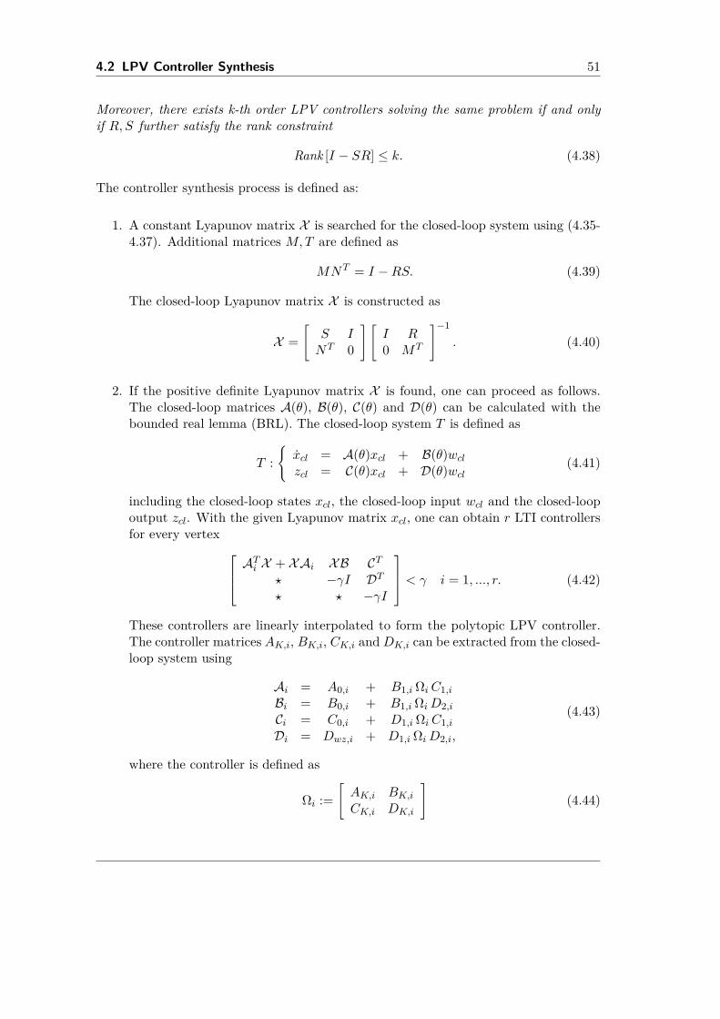
4.2 LPV Controller Synthesis 51
Moreover, there exists k-th order LPV controllers solving the same problem if and onlyif R,S further satisfy the rank constraint
Rank [I − SR] ≤ k. (4.38)
The controller synthesis process is defined as:
1. A constant Lyapunov matrix X is searched for the closed-loop system using (4.35-4.37). Additional matrices M,T are defined as
MNT = I −RS. (4.39)
The closed-loop Lyapunov matrix X is constructed as
X =[
S INT 0
] [I R0 MT
]−1
. (4.40)
2. If the positive definite Lyapunov matrix X is found, one can proceed as follows.The closed-loop matrices A(θ), B(θ), C(θ) and D(θ) can be calculated with thebounded real lemma (BRL). The closed-loop system T is defined as
T :xcl = A(θ)xcl + B(θ)wclzcl = C(θ)xcl + D(θ)wcl
(4.41)
including the closed-loop states xcl, the closed-loop input wcl and the closed-loopoutput zcl. With the given Lyapunov matrix xcl, one can obtain r LTI controllersfor every vertex ATi X + XAi XB CT
? −γI DT? ? −γI
< γ i = 1, ..., r. (4.42)
These controllers are linearly interpolated to form the polytopic LPV controller.The controller matrices AK,i, BK,i, CK,i andDK,i can be extracted from the closed-loop system using
Ai = A0,i + B1,i ΩiC1,iBi = B0,i + B1,i ΩiD2,iCi = C0,i + D1,i ΩiC1,iDi = Dwz,i + D1,i ΩiD2,i,
(4.43)
where the controller is defined as
Ωi :=[AK,i BK,iCK,i DK,i
](4.44)
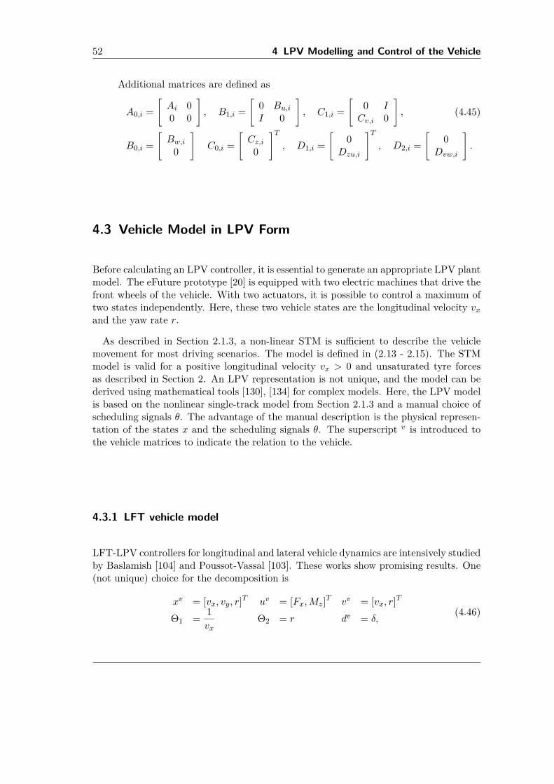
52 4 LPV Modelling and Control of the Vehicle
Additional matrices are defined as
A0,i =[Ai 00 0
], B1,i =
[0 Bu,iI 0
], C1,i =
[0 ICv,i 0
], (4.45)
B0,i =[Bw,i
0
]C0,i =
[Cz,i
0
]T, D1,i =
[0
Dzu,i
]T, D2,i =
[0
Dvw,i
].
4.3 Vehicle Model in LPV Form
Before calculating an LPV controller, it is essential to generate an appropriate LPV plantmodel. The eFuture prototype [20] is equipped with two electric machines that drive thefront wheels of the vehicle. With two actuators, it is possible to control a maximum oftwo states independently. Here, these two vehicle states are the longitudinal velocity vxand the yaw rate r.
As described in Section 2.1.3, a non-linear STM is sufficient to describe the vehiclemovement for most driving scenarios. The model is defined in (2.13 - 2.15). The STMmodel is valid for a positive longitudinal velocity vx > 0 and unsaturated tyre forcesas described in Section 2. An LPV representation is not unique, and the model can bederived using mathematical tools [130], [134] for complex models. Here, the LPV modelis based on the nonlinear single-track model from Section 2.1.3 and a manual choice ofscheduling signals θ. The advantage of the manual description is the physical represen-tation of the states x and the scheduling signals θ. The superscript v is introduced tothe vehicle matrices to indicate the relation to the vehicle.
4.3.1 LFT vehicle model
LFT-LPV controllers for longitudinal and lateral vehicle dynamics are intensively studiedby Baslamish [104] and Poussot-Vassal [103]. These works show promising results. One(not unique) choice for the decomposition is
xv = [vx, vy, r]T uv = [Fx,Mz]T vv = [vx, r]T
Θ1 = 1vx
Θ2 = r dv = δ,(4.46)
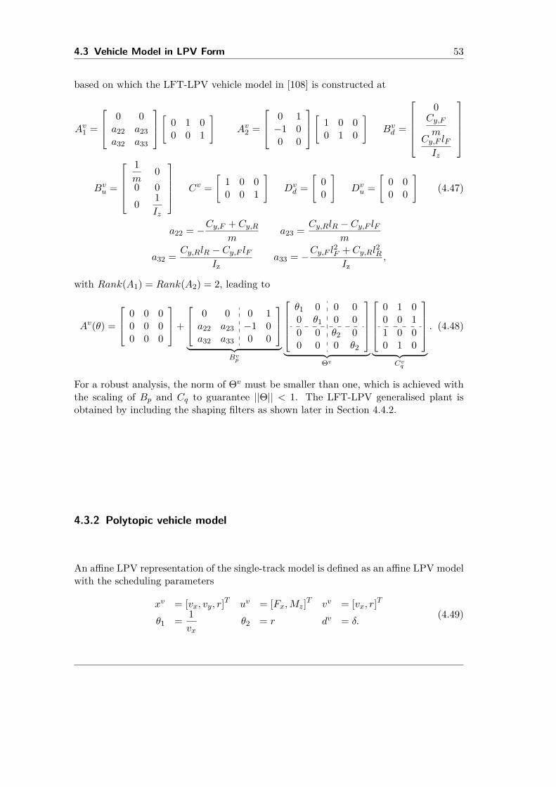
4.3 Vehicle Model in LPV Form 53
based on which the LFT-LPV vehicle model in [108] is constructed at
Av1 =
0 0a22 a23a32 a33
[ 0 1 00 0 1
]Av2 =
0 1−1 00 0
[ 1 0 00 1 0
]Bvd =
0
Cy,Fm
Cy,F lFIz
Bvu =
1m
00 00 1
Iz
Cv =[
1 0 00 0 1
]Dvd =
[00
]Dvu =
[0 00 0
](4.47)
a22 = −Cy,F + Cy,Rm
a23 = Cy,RlR − Cy,F lFm
a32 = Cy,RlR − Cy,F lFIz
a33 = −Cy,F l2F + Cy,Rl
2R
Iz,
with Rank(A1) = Rank(A2) = 2, leading to
Av(θ) =
0 0 00 0 00 0 0
+
0 0 0 1a22 a23 −1 0a32 a33 0 0
︸ ︷︷ ︸
Bvp
θ1 0 0 00 θ1 0 00 0 θ2 00 0 0 θ2
︸ ︷︷ ︸
Θv
0 1 00 0 11 0 00 1 0
︸ ︷︷ ︸
Cvq
. (4.48)
For a robust analysis, the norm of Θv must be smaller than one, which is achieved withthe scaling of Bp and Cq to guarantee ||Θ|| < 1. The LFT-LPV generalised plant isobtained by including the shaping filters as shown later in Section 4.4.2.
4.3.2 Polytopic vehicle model
An affine LPV representation of the single-track model is defined as an affine LPV modelwith the scheduling parameters
xv = [vx, vy, r]T uv = [Fx,Mz]T vv = [vx, r]T
θ1 = 1vx
θ2 = r dv = δ.(4.49)
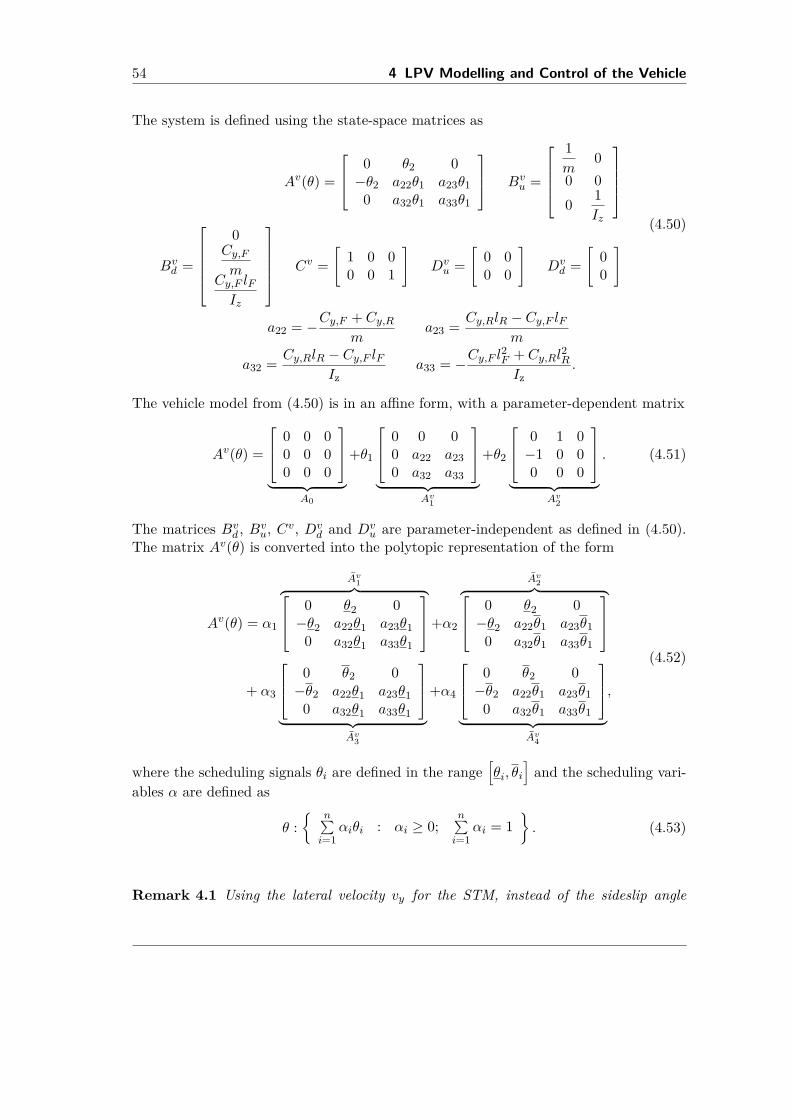
54 4 LPV Modelling and Control of the Vehicle
The system is defined using the state-space matrices as
Av(θ) =
0 θ2 0−θ2 a22θ1 a23θ1
0 a32θ1 a33θ1
Bvu =
1m
00 00 1
Iz
Bvd =
0
Cy,Fm
Cy,F lFIz
Cv =[
1 0 00 0 1
]Dvu =
[0 00 0
]Dvd =
[00
] (4.50)
a22 = −Cy,F + Cy,Rm
a23 = Cy,RlR − Cy,F lFm
a32 = Cy,RlR − Cy,F lFIz
a33 = −Cy,F l2F + Cy,Rl
2R
Iz.
The vehicle model from (4.50) is in an affine form, with a parameter-dependent matrix
Av(θ) =
0 0 00 0 00 0 0
︸ ︷︷ ︸
A0
+θ1
0 0 00 a22 a230 a32 a33
︸ ︷︷ ︸
Av1
+θ2
0 1 0−1 0 00 0 0
︸ ︷︷ ︸
Av2
. (4.51)
The matrices Bvd , Bv
u, Cv, Dvd and Dv
u are parameter-independent as defined in (4.50).The matrix Av(θ) is converted into the polytopic representation of the form
Av(θ) = α1
Av1︷ ︸︸ ︷ 0 θ2 0−θ2 a22θ1 a23θ1
0 a32θ1 a33θ1
+α2
Av2︷ ︸︸ ︷ 0 θ2 0−θ2 a22θ1 a23θ1
0 a32θ1 a33θ1
+ α3
0 θ2 0−θ2 a22θ1 a23θ1
0 a32θ1 a33θ1
︸ ︷︷ ︸
Av3
+α4
0 θ2 0−θ2 a22θ1 a23θ1
0 a32θ1 a33θ1
︸ ︷︷ ︸
Av4
,
(4.52)
where the scheduling signals θi are defined in the range[θi, θi
]and the scheduling vari-
ables α are defined as
θ : n∑
i=1αiθi : αi ≥ 0;
n∑i=1
αi = 1. (4.53)
Remark 4.1 Using the lateral velocity vy for the STM, instead of the sideslip angle
4.4 Torque Vectoring Controller Design 55
β, has the advantage that the matrix B is parameter-independent. Only the A matrixdepends on θ.
Remark 4.2 The lateral velocity vy or sideslip angle β are not considered as controlledoutputs because it is not possible to control the yaw-rate and the sideslip angle inde-pendently, using only the yaw moment Mz. Trying to control both properties leads toa functionally uncontrollable [23] system with uncontrollable directions. Controlling thelateral velocity (or the sideslip angle) and the yaw rate is possible only by including anadditional device like an active steering system.
4.4 Torque Vectoring Controller Design
A mixed-sensitivity loop shaping design is chosen for the torque vectoring controllerdesign. Even though for time-varying systems transfer functions and poles or zeros arenot defined, it is meaningful to shape the frequency response of sensitivity functionswhen the parameters are frozen. Dynamic shaping filters are designed in Section 4.4.1and combined with the vehicle model from Section 4.3 to the generalised plant in Section4.4.2. The synthesis procedure from Section 4.2 is applied to the generalised plant.Additional synthesis constraints are discussed in Section 4.4.3, and these constraints areincluded in the design. All steps are performed both for the LFT-LPV and the polytopicLPV design.
4.4.1 Shaping filter
Shaping filters are used in mixed-sensitivity designs to realise frequency-dependent per-formance requirements. Different priorities between control error and control input arerealised. As in [135], the sensitivity of the closed-loop system is shaped using a low-passfilter WS to reduce the steady state error and to obtain good tracking performance forlow frequencies. The control-sensitivity is shaped using the high-pass filterWC to reducethe control effort, which reduces the energy consumption of the system and is used todeal with actuator limitations.
Shaping filters - LFT
For the torque vectoring controller in LFT-LPV form, the sensitivity filter WS and thecontrol-sensitivity filter WC are defined as first order filters which for frozen values of
56 4 LPV Modelling and Control of the Vehicle
θ1 can be represented as
WS(s) =
1MS
1
Θ1s
ωS1+ 1
0
0 1MS
2
1s
ωS2+ 1
(4.54)
WC(s) =
1MC
s
ωC+ 1
s
c ωC+ 1
[ 1 00 1
]. (4.55)
The scheduling parameter Θ1 can be used for parameter-dependent shaping filters be-cause the requirements for longitudinal and lateral response varies strongly with thevelocity of the vehicle, as described in Section 3.5.Often, shaping filters are parameter-independent as in [104], [103], but parameter-
dependent shaping filters reduce conservatism and improve the torque vectoring con-troller, as shown by Bartels et al. [108]. The shaping filters WS(θ) and WC(θ) can berepresented as lower LFT-LPVs (definition in [133]) in the form xS
zS
qS
=
AS BSw BS
p
CSz DSzw DS
zp
CSq DSqw DS
qp
xS
wS
pS
(4.56)
pS = ΘSqS (4.57)
xC
zC
qC
=
AC BCw BC
p
CCz DCzw DC
zp
CCq DCqw DC
qp
xC
wC
pC
(4.58)
pC = ΘCqC . (4.59)
Shaping filters - polytopic LPV
In most polytopic LPV controllers, such as [129], [136] shaping filters are independent ofscheduling parameters θ. The transfer functions of the filters are pure gains or first ordersystems. For torque vectoring, the requirements change with the longitudinal velocity ofthe vehicle, as described in 3.5. The shaping filters penalise the yaw rate error at highvelocities and relax the lateral constraints for low velocities. The number of schedulingparameters r must be as small as possible to minimise the computational effort of themicrocontroller. The filters are designed with a parameter-dependent A-matrix A(θ)and constant B, C and D matrices.As recommended in [23], dynamic components of filters are realised using first order,
low-pass filters for sensitivity and first order, high-pass filters for control sensitivity. The
4.4 Torque Vectoring Controller Design 57
sensitivity shaping filter WS is defined as
WS(θ) = CS(sI −AS(θ))−1BS +DS , (4.60)
where
AS(θ) =[−ωS1 0
0 −θ1ωS2
], BS =
[1 00 1
], (4.61)
CS =
ωS1MS
10
0 ωS2MS
2
, DS =[
0 00 0
].
The control sensitivity filter WC is defined as
WC(θ) = CC(sI −AC(θ))−1BC +DC , (4.62)
where
AC(θ) =[−c ωC1 0
0 −c (0.995 + 0.001θ1)ωC2
], BC =
[1 00 1
](4.63)
CC = −
c ωC1 (c− 1)
MC1
0
0 c ωC2 (c− 1)MC
2
, DC =
c
MC1
0
0 c
MC2
.With these structures, parameter-dependent shaping filters can be constructed that fol-low the assumptions of the polytopic LPV controller design of Apkarian et al. [129].
4.4.2 Generalised plant
For LPV control synthesis, a generalised plant, as shown in Figure 4.1, must be defined.The generalised plant contains the vehicle model and shaping filters for closed-looptuning. Inputs to the generalised plant are exogenous signal w, such as disturbances,reference and noise signals, and the control input u from the controller. Outputs of thegeneralised plant are the performance signal z, and the input of the controller v. Thecontroller input v may consist of control error signals, measured signals or disturbancesignals, which should be routed to the controller. Generalised plants are presented forLFT-LPV and polytopic LPV controllers.The mixed-sensitivity design penalises the control error e and the control input u
with the parameter-dependent shaping filters WS(θ) and WC(θ). The filters are usedto shape closed-loop performance and to find an appropriate trade-off between trackingperformance and control effort. Here, a disturbance term d is introduced to handle thechange of the front tyre steering angle.
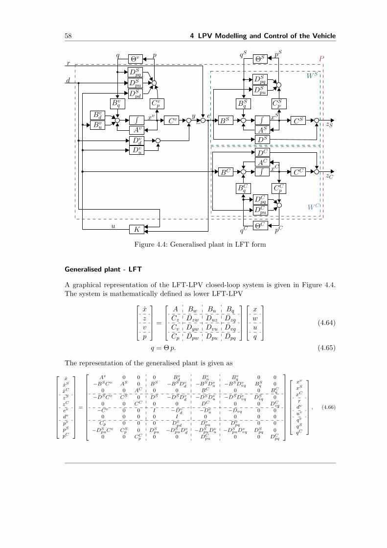
58 4 LPV Modelling and Control of the Vehicle
Θv
∫ CvpBvq
Cv
Av
Dvd
Dvu
y ezS
Bvd
Bvu
K
BC
−
d
r
xv
pq
u
P
AS
∫ CSpBSq
pSqS ΘS
BS CS
DS
ACDC
∫CC
CCpBCq
ΘC
zC
WS
WC
DSpq
DSpu
DCpq
DCpu
DSpq
DSpu
DSpd
pCqC
xC
xS
Figure 4.4: Generalised plant in LFT form
Generalised plant - LFT
A graphical representation of the LFT-LPV closed-loop system is given in Figure 4.4.The system is mathematically defined as lower LFT-LPV
x
z
v
p
=
A Bw Bu BqCz Dzw Duz Dzq
Cv Dyw Dvu Dvq
Cp Dpw Dpu Dpq
x
w
u
q
(4.64)
q = Θ p. (4.65)
The representation of the generalised plant is given as
xxS
xC
zS
zC
ev
dv
pv
pS
pC
=
Av 0 0 0 Bvd Bvu Bvq 0 0−BSCv AS 0 BS −BSDvd −BSDvu −BSDvvq BSq 0
0 0 AC 0 0 BC 0 0 BCq−DSCv CS 0 DS −DSDvd −DSDvu −DSDvvq DSzq 0
0 0 CC 0 0 DC 0 0 DCzq−Cv 0 0 I −Dvd −Dvu −Dvq 0 0
0 0 0 0 I 0 0 0 0Cp 0 0 0 Dvpd Dvpu Dvpq 0 0
−DSpuCv CSp 0 DSpu −DSpuDvd −DSpuDvu −DSpuDvvq DSpq 00 0 CCp 0 0 DCpu 0 0 DCpq
xv
xS
xC
rdv
uv
qv
qS
qC
, (4.66)
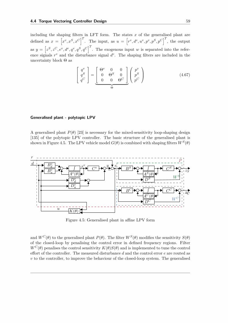
4.4 Torque Vectoring Controller Design 59
including the shaping filters in LFT form. The states x of the generalised plant aredefined as x =
[xv, xS , xC
]T. The input, as u =
[rv, dv, uv, pv, pS , pC
]T, the output
as y =[zS , zC , ev, dv, qv, qS , qC
]T. The exogenous input w is separated into the refer-
ence signals rv and the disturbance signal dv. The shaping filters are included in theuncertainty block Θ as qv
qS
qC
=
Θv 0 00 ΘS 00 0 ΘC
︸ ︷︷ ︸
Θ
pv
pS
pC
(4.67)
Generalised plant - polytopic LPV
A generalised plant P (θ) [23] is necessary for the mixed-sensitivity loop-shaping design[135] of the polytopic LPV controller. The basic structure of the generalised plant isshown in Figure 4.5. The LPV vehicle modelG(θ) is combined with shaping filtersWS(θ)
∫Cv
Av(θ)Dvd
Dvu
y ezS
Bvd
Bvu
K(θ)
−d
r
xv
u
P
AS(θ)
∫BS CS
DS
zC
WS
WC
zCAC(θ)
∫BC CC
DC
Figure 4.5: Generalised plant in affine LPV form
and WC(θ) to the generalised plant P (θ). The filter WS(θ) modifies the sensitivity S(θ)of the closed-loop by penalising the control error in defined frequency regions. FilterWC(θ) penalises the control sensitivity K(θ)S(θ) and is implemented to tune the controleffort of the controller. The measured disturbance d and the control error e are routed asv to the controller, to improve the behaviour of the closed-loop system. The generalised
60 4 LPV Modelling and Control of the Vehicle
plant P (θ) from (4.11) is defined as
xv
xS
xC
zS
zC
ev
dv
=
Av(θ) 0 0 0 Bvd Bv
u
−BSCc AS(θ) 0 BS −BSDvd −BSDv
u
0 0 AC(θ) 0 0 BC
−DSCv CS 0 DS −DSDvd −DSDv
u
0 0 CC 0 0 DC
−CC 0 0 I −Dvd −Dv
u
0 0 0 0 I 0
xv
xS
xC
rv
dv
uv
. (4.68)
Shaping filters are often parameter-independent, as in [105], [120], [129]. As discussedin the LFT-LPV controller design, it can be advantageous to use parameter-dependentshaping filters.
4.4.3 Additional constraints
The LFT-LPV and the polytopic LPV controller synthesis procedures, described in 4.2,generate continuous-time controllers for the LPV torque vectoring controller which guar-antee stability and performance. To implement the control algorithm, some additionalconstraints should be included in the controller design.
Spectral radius constraint
Controller poles (for frozen parameters) may turn out to be located far in the left halfplane (LHP). Far LHP poles are not problematic in continuous-time simulations, butthe continuous-time controller design must be converted into a discrete-time design forpractical implementation. In fact, it is not possible to represent excessively fast controllerpoles correctly with a defined sample time Td and a quantization step h. The mappingof pole locations from continuous-time to discrete-time is given by
z = esTd (4.69)
where s is the location in the continuous complex plane. The sampling time is defined asTd, and the location in the discrete complex plane is defined as z. The microcontrollerused limits the system to 32 bits and a sample time of 0.01s. Including a safety factorsF of 10, the maximum pole location in continuous-time is given as
s = ln (sF · z) 1Td
(4.70)
s = ln (10 · 2−31) 10.01 = −1918.5. (4.71)
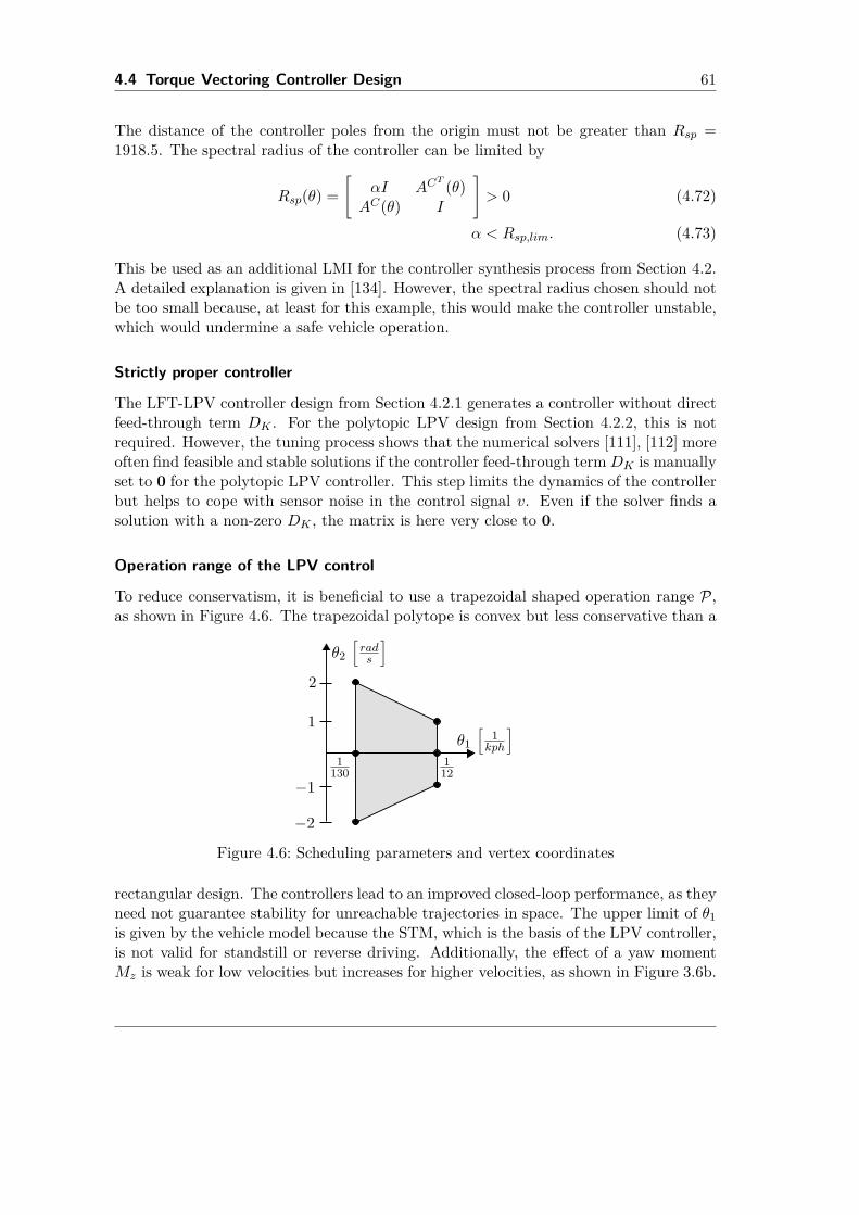
4.4 Torque Vectoring Controller Design 61
The distance of the controller poles from the origin must not be greater than Rsp =1918.5. The spectral radius of the controller can be limited by
Rsp(θ) =[
αI ACT (θ)
AC(θ) I
]> 0 (4.72)
α < Rsp,lim. (4.73)
This be used as an additional LMI for the controller synthesis process from Section 4.2.A detailed explanation is given in [134]. However, the spectral radius chosen should notbe too small because, at least for this example, this would make the controller unstable,which would undermine a safe vehicle operation.
Strictly proper controller
The LFT-LPV controller design from Section 4.2.1 generates a controller without directfeed-through term DK . For the polytopic LPV design from Section 4.2.2, this is notrequired. However, the tuning process shows that the numerical solvers [111], [112] moreoften find feasible and stable solutions if the controller feed-through termDK is manuallyset to 0 for the polytopic LPV controller. This step limits the dynamics of the controllerbut helps to cope with sensor noise in the control signal v. Even if the solver finds asolution with a non-zero DK , the matrix is here very close to 0.
Operation range of the LPV control
To reduce conservatism, it is beneficial to use a trapezoidal shaped operation range P,as shown in Figure 4.6. The trapezoidal polytope is convex but less conservative than a
θ2[rads
]2
1
−1
−2
θ1[
1kph
]1
130112
Figure 4.6: Scheduling parameters and vertex coordinates
rectangular design. The controllers lead to an improved closed-loop performance, as theyneed not guarantee stability for unreachable trajectories in space. The upper limit of θ1is given by the vehicle model because the STM, which is the basis of the LPV controller,is not valid for standstill or reverse driving. Additionally, the effect of a yaw momentMz is weak for low velocities but increases for higher velocities, as shown in Figure 3.6b.
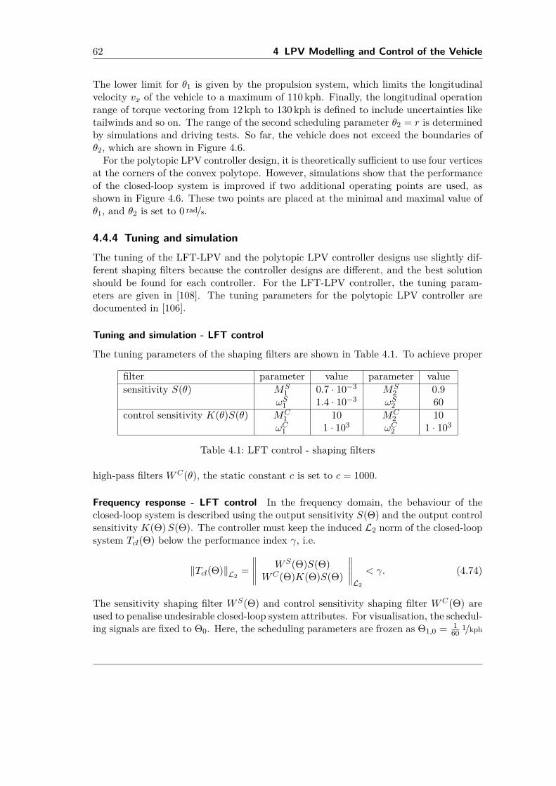
62 4 LPV Modelling and Control of the Vehicle
The lower limit for θ1 is given by the propulsion system, which limits the longitudinalvelocity vx of the vehicle to a maximum of 110 kph. Finally, the longitudinal operationrange of torque vectoring from 12 kph to 130 kph is defined to include uncertainties liketailwinds and so on. The range of the second scheduling parameter θ2 = r is determinedby simulations and driving tests. So far, the vehicle does not exceed the boundaries ofθ2, which are shown in Figure 4.6.For the polytopic LPV controller design, it is theoretically sufficient to use four vertices
at the corners of the convex polytope. However, simulations show that the performanceof the closed-loop system is improved if two additional operating points are used, asshown in Figure 4.6. These two points are placed at the minimal and maximal value ofθ1, and θ2 is set to 0 rad/s.
4.4.4 Tuning and simulationThe tuning of the LFT-LPV and the polytopic LPV controller designs use slightly dif-ferent shaping filters because the controller designs are different, and the best solutionshould be found for each controller. For the LFT-LPV controller, the tuning param-eters are given in [108]. The tuning parameters for the polytopic LPV controller aredocumented in [106].
Tuning and simulation - LFT control
The tuning parameters of the shaping filters are shown in Table 4.1. To achieve proper
filter parameter value parameter valuesensitivity S(θ) MS
1 0.7 · 10−3 MS2 0.9
ωS1 1.4 · 10−3 ωS2 60control sensitivity K(θ)S(θ) MC
1 10 MC2 10
ωC1 1 · 103 ωC2 1 · 103
Table 4.1: LFT control - shaping filters
high-pass filters WC(θ), the static constant c is set to c = 1000.
Frequency response - LFT control In the frequency domain, the behaviour of theclosed-loop system is described using the output sensitivity S(Θ) and the output controlsensitivity K(Θ)S(Θ). The controller must keep the induced L2 norm of the closed-loopsystem Tcl(Θ) below the performance index γ, i.e.
‖Tcl(Θ)‖L2=∥∥∥∥∥ WS(Θ)S(Θ)WC(Θ)K(Θ)S(Θ)
∥∥∥∥∥L2
< γ. (4.74)
The sensitivity shaping filter WS(Θ) and control sensitivity shaping filter WC(Θ) areused to penalise undesirable closed-loop system attributes. For visualisation, the schedul-ing signals are fixed to Θ0. Here, the scheduling parameters are frozen as Θ1,0 = 1
601/kph
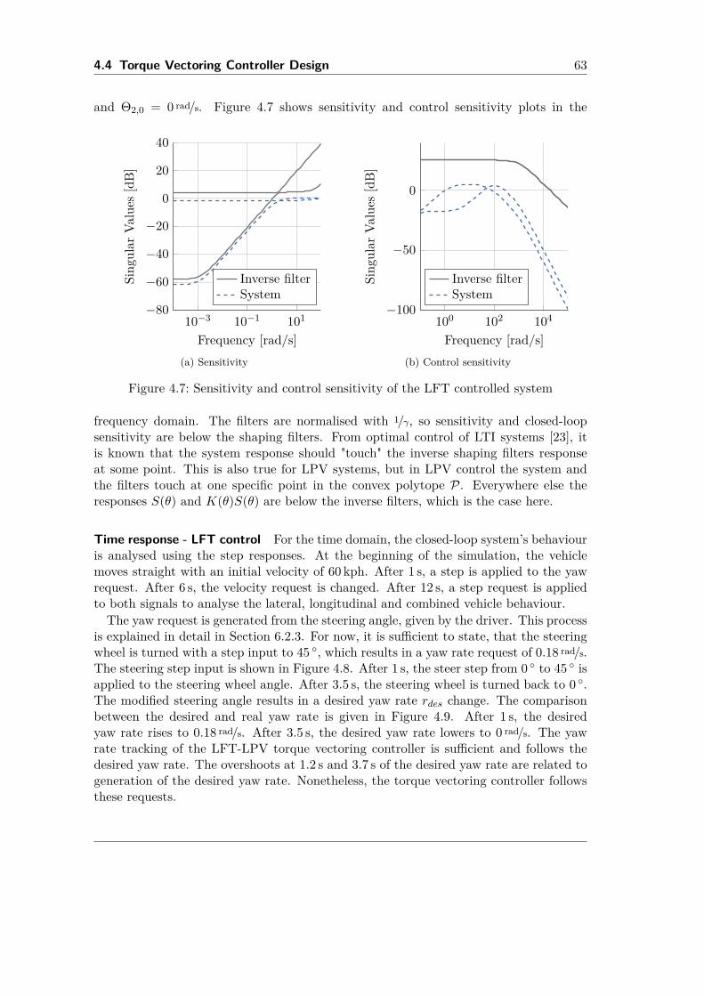
4.4 Torque Vectoring Controller Design 63
and Θ2,0 = 0 rad/s. Figure 4.7 shows sensitivity and control sensitivity plots in the
10−3 10−1 101−80
−60
−40
−20
0
20
40
Frequency [rad/s]
Sing
ular
Values
[dB]
Inverse filterSystem
(a) Sensitivity
100 102 104−100
−50
0
Frequency [rad/s]
Sing
ular
Values
[dB]
Inverse filterSystem
(b) Control sensitivity
Figure 4.7: Sensitivity and control sensitivity of the LFT controlled system
frequency domain. The filters are normalised with 1/γ, so sensitivity and closed-loopsensitivity are below the shaping filters. From optimal control of LTI systems [23], itis known that the system response should "touch" the inverse shaping filters responseat some point. This is also true for LPV systems, but in LPV control the system andthe filters touch at one specific point in the convex polytope P. Everywhere else theresponses S(θ) and K(θ)S(θ) are below the inverse filters, which is the case here.
Time response - LFT control For the time domain, the closed-loop system’s behaviouris analysed using the step responses. At the beginning of the simulation, the vehiclemoves straight with an initial velocity of 60 kph. After 1 s, a step is applied to the yawrequest. After 6 s, the velocity request is changed. After 12 s, a step request is appliedto both signals to analyse the lateral, longitudinal and combined vehicle behaviour.The yaw request is generated from the steering angle, given by the driver. This process
is explained in detail in Section 6.2.3. For now, it is sufficient to state, that the steeringwheel is turned with a step input to 45 , which results in a yaw rate request of 0.18 rad/s.The steering step input is shown in Figure 4.8. After 1 s, the steer step from 0 to 45 isapplied to the steering wheel angle. After 3.5 s, the steering wheel is turned back to 0 .The modified steering angle results in a desired yaw rate rdes change. The comparisonbetween the desired and real yaw rate is given in Figure 4.9. After 1 s, the desiredyaw rate rises to 0.18 rad/s. After 3.5 s, the desired yaw rate lowers to 0 rad/s. The yawrate tracking of the LFT-LPV torque vectoring controller is sufficient and follows thedesired yaw rate. The overshoots at 1.2 s and 3.7 s of the desired yaw rate are related togeneration of the desired yaw rate. Nonetheless, the torque vectoring controller followsthese requests.
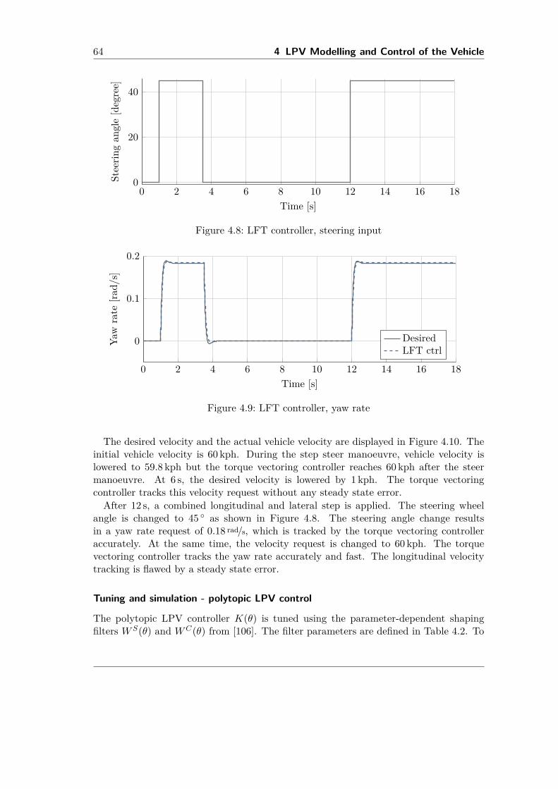
64 4 LPV Modelling and Control of the Vehicle
0 2 4 6 8 10 12 14 16 180
20
40
Time [s]
Stee
ring
angl
e[d
egre
e]
Figure 4.8: LFT controller, steering input
0 2 4 6 8 10 12 14 16 18
0
0.1
0.2
Time [s]
Yaw
rate
[rad/
s]
DesiredLFT ctrl
Figure 4.9: LFT controller, yaw rate
The desired velocity and the actual vehicle velocity are displayed in Figure 4.10. Theinitial vehicle velocity is 60 kph. During the step steer manoeuvre, vehicle velocity islowered to 59.8 kph but the torque vectoring controller reaches 60 kph after the steermanoeuvre. At 6 s, the desired velocity is lowered by 1 kph. The torque vectoringcontroller tracks this velocity request without any steady state error.After 12 s, a combined longitudinal and lateral step is applied. The steering wheel
angle is changed to 45 as shown in Figure 4.8. The steering angle change resultsin a yaw rate request of 0.18 rad/s, which is tracked by the torque vectoring controlleraccurately. At the same time, the velocity request is changed to 60 kph. The torquevectoring controller tracks the yaw rate accurately and fast. The longitudinal velocitytracking is flawed by a steady state error.
Tuning and simulation - polytopic LPV control
The polytopic LPV controller K(θ) is tuned using the parameter-dependent shapingfilters WS(θ) and WC(θ) from [106]. The filter parameters are defined in Table 4.2. To
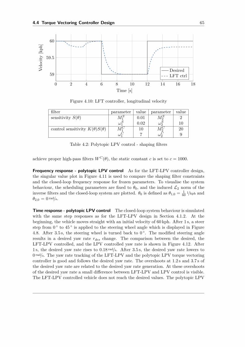
4.4 Torque Vectoring Controller Design 65
0 2 4 6 8 10 12 14 16 18
59
59.5
60
Time [s]
Velo
city
[kph
]
DesiredLFT ctrl
Figure 4.10: LFT controller, longitudinal velocity
filter parameter value parameter valuesensitivity S(θ) MS
1 0.01 MS2 2
ωS1 0.02 ωS2 10control sensitivity K(θ)S(θ) MC
1 10 MC2 20
ωC1 7 ωC2 9
Table 4.2: Polytopic LPV control - shaping filters
achieve proper high-pass filters WC(θ), the static constant c is set to c = 1000.
Frequency response - polytopic LPV control As for the LFT-LPV controller design,the singular value plot in Figure 4.11 is used to compare the shaping filter constraintsand the closed-loop frequency response for frozen parameters. To visualise the systembehaviour, the scheduling parameters are fixed to θ0, and the induced L2 norm of theinverse filters and the closed-loop system are plotted. θ0 is defined as θ1,0 = 1
601/kph and
θ2,0 = 0 rad/s.
Time response - polytopic LPV control The closed-loop system behaviour is simulatedwith the same step responses as for the LFT-LPV design in Section 4.1.2. At thebeginning, the vehicle moves straight with an initial velocity of 60 kph. After 1 s, a steerstep from 0 to 45 is applied to the steering wheel angle which is displayed in Figure4.8. After 3.5 s, the steering wheel is turned back to 0 . The modified steering angleresults in a desired yaw rate rdes change. The comparison between the desired, theLFT-LPV controlled, and the LPV controlled yaw rate is shown in Figure 4.12. After1 s, the desired yaw rate rises to 0.18 rad/s. After 3.5 s, the desired yaw rate lowers to0 rad/s. The yaw rate tracking of the LFT-LPV and the polytopic LPV torque vectoringcontroller is good and follows the desired yaw rate. The overshoots at 1.2 s and 3.7 s ofthe desired yaw rate are related to the desired yaw rate generation. At these overshootsof the desired yaw rate a small difference between LFT-LPV and LPV control is visible.The LFT-LPV controlled vehicle does not reach the desired values. The polytopic LPV
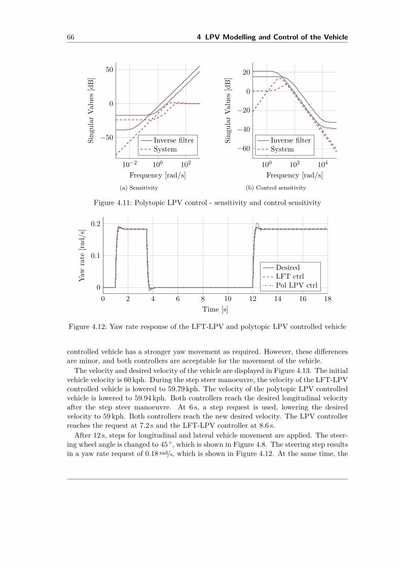
66 4 LPV Modelling and Control of the Vehicle
10−2 100 102
−50
0
50
Frequency [rad/s]
Sing
ular
Values
[dB]
Inverse filterSystem
(a) Sensitivity
100 102 104
−60
−40
−20
0
20
Frequency [rad/s]
Sing
ular
Values
[dB]
Inverse filterSystem
(b) Control sensitivity
Figure 4.11: Polytopic LPV control - sensitivity and control sensitivity
0 2 4 6 8 10 12 14 16 180
0.1
0.2
Time [s]
Yaw
rate
[rad/
s]
DesiredLFT ctrlPol LPV ctrl
Figure 4.12: Yaw rate response of the LFT-LPV and polytopic LPV controlled vehicle
controlled vehicle has a stronger yaw movement as required. However, these differencesare minor, and both controllers are acceptable for the movement of the vehicle.The velocity and desired velocity of the vehicle are displayed in Figure 4.13. The initial
vehicle velocity is 60 kph. During the step steer manoeuvre, the velocity of the LFT-LPVcontrolled vehicle is lowered to 59.79 kph. The velocity of the polytopic LPV controlledvehicle is lowered to 59.94 kph. Both controllers reach the desired longitudinal velocityafter the step steer manoeuvre. At 6 s, a step request is used, lowering the desiredvelocity to 59 kph. Both controllers reach the new desired velocity. The LPV controllerreaches the request at 7.2 s and the LFT-LPV controller at 8.6 s.After 12 s, steps for longitudinal and lateral vehicle movement are applied. The steer-
ing wheel angle is changed to 45 , which is shown in Figure 4.8. The steering step resultsin a yaw rate request of 0.18 rad/s, which is shown in Figure 4.12. At the same time, the
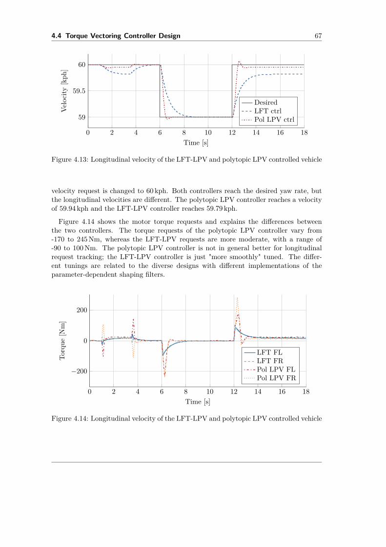
4.4 Torque Vectoring Controller Design 67
0 2 4 6 8 10 12 14 16 18
59
59.5
60
Time [s]
Velo
city
[kph
]
DesiredLFT ctrlPol LPV ctrl
Figure 4.13: Longitudinal velocity of the LFT-LPV and polytopic LPV controlled vehicle
velocity request is changed to 60 kph. Both controllers reach the desired yaw rate, butthe longitudinal velocities are different. The polytopic LPV controller reaches a velocityof 59.94 kph and the LFT-LPV controller reaches 59.79 kph.
Figure 4.14 shows the motor torque requests and explains the differences betweenthe two controllers. The torque requests of the polytopic LPV controller vary from-170 to 245Nm, whereas the LFT-LPV requests are more moderate, with a range of-90 to 100Nm. The polytopic LPV controller is not in general better for longitudinalrequest tracking; the LFT-LPV controller is just "more smoothly" tuned. The differ-ent tunings are related to the diverse designs with different implementations of theparameter-dependent shaping filters.
0 2 4 6 8 10 12 14 16 18
−200
0
200
Time [s]
Torq
ue[N
m]
LFT FLLFT FRPol LPV FLPol LPV FR
Figure 4.14: Longitudinal velocity of the LFT-LPV and polytopic LPV controlled vehicle
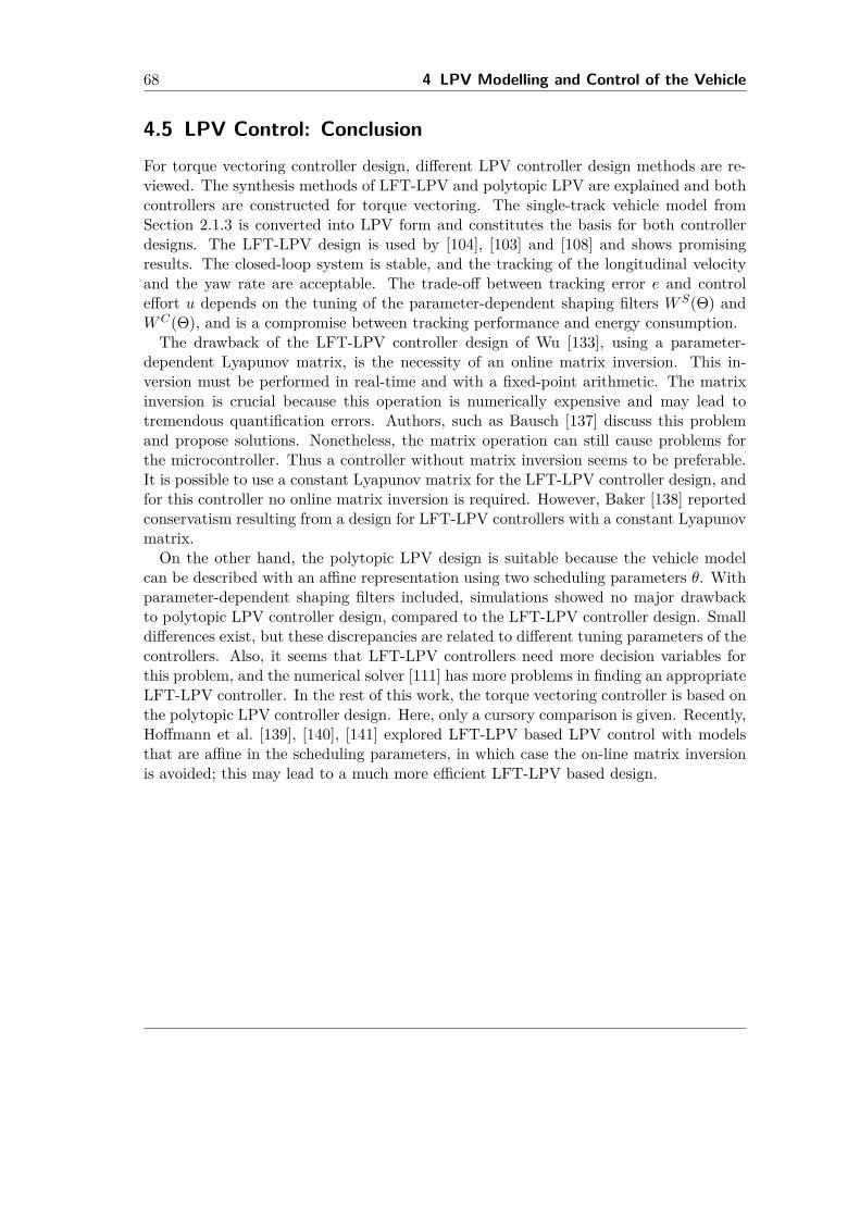
68 4 LPV Modelling and Control of the Vehicle
4.5 LPV Control: ConclusionFor torque vectoring controller design, different LPV controller design methods are re-viewed. The synthesis methods of LFT-LPV and polytopic LPV are explained and bothcontrollers are constructed for torque vectoring. The single-track vehicle model fromSection 2.1.3 is converted into LPV form and constitutes the basis for both controllerdesigns. The LFT-LPV design is used by [104], [103] and [108] and shows promisingresults. The closed-loop system is stable, and the tracking of the longitudinal velocityand the yaw rate are acceptable. The trade-off between tracking error e and controleffort u depends on the tuning of the parameter-dependent shaping filters WS(Θ) andWC(Θ), and is a compromise between tracking performance and energy consumption.The drawback of the LFT-LPV controller design of Wu [133], using a parameter-
dependent Lyapunov matrix, is the necessity of an online matrix inversion. This in-version must be performed in real-time and with a fixed-point arithmetic. The matrixinversion is crucial because this operation is numerically expensive and may lead totremendous quantification errors. Authors, such as Bausch [137] discuss this problemand propose solutions. Nonetheless, the matrix operation can still cause problems forthe microcontroller. Thus a controller without matrix inversion seems to be preferable.It is possible to use a constant Lyapunov matrix for the LFT-LPV controller design, andfor this controller no online matrix inversion is required. However, Baker [138] reportedconservatism resulting from a design for LFT-LPV controllers with a constant Lyapunovmatrix.On the other hand, the polytopic LPV design is suitable because the vehicle model
can be described with an affine representation using two scheduling parameters θ. Withparameter-dependent shaping filters included, simulations showed no major drawbackto polytopic LPV controller design, compared to the LFT-LPV controller design. Smalldifferences exist, but these discrepancies are related to different tuning parameters of thecontrollers. Also, it seems that LFT-LPV controllers need more decision variables forthis problem, and the numerical solver [111] has more problems in finding an appropriateLFT-LPV controller. In the rest of this work, the torque vectoring controller is based onthe polytopic LPV controller design. Here, only a cursory comparison is given. Recently,Hoffmann et al. [139], [140], [141] explored LFT-LPV based LPV control with modelsthat are affine in the scheduling parameters, in which case the on-line matrix inversionis avoided; this may lead to a much more efficient LFT-LPV based design.
5 Torque and Slip Limiter
The LPV controller from Chapter 4 achieves acceptable simulation results for variousdriving conditions. However, the vehicle performance is inadequate if the vehicle hasto accelerate or brake strongly or if extreme steering manoeuvres are executed. If suchmanoeuvres are performed, the vehicle oscillates, or even worse, becomes unstable. Thecause of this problem is the physical limitation of the drivetrain.As mentioned in Section 2.2.2, the maximum torque, the maximum torque slew rate,
and the maximum power of the electric machines are limited. If the controller requestsmore motor torque than is physically possible, the actuators reach the limits of saturationand the controller starts to "windup". Controller windup degrades the performance ofthe controller and can make the closed-loop system unstable. Windup effects have beendiscussed since the 1930s and controller windup is probably the root cause of manycatastrophes, such as the nuclear accident in Chernobyl in 1986 [142] or the crash of jetfighters [143].In the eFuture prototype, the motor torque and wheel slip limiter (TSL) is imple-
mented to improve the performance and safety of the electric vehicle and to preventthe torque vectoring controller from experiencing windup. Section 5.1 gives an overviewof standard strategies for coping with actuator limitations. In Section 5.2, anti-windupstrategies are applied to the torque vectoring controller. In Section 5.3, the anti-windupscheme is extended to limit tyre slip and enhance the anti-windup compensator for theTSL algorithm. Simulation results are discussed in Section 5.4, and conclusions are givenin Section 5.5.
5.1 Anti-Windup Compensator - OverviewThe problem of windup for proportional-integral (PI) controllers was practically recog-nised in the 1930s, and has been theoretically discussed since the 1950s. One solution tothe windup problem is to reconfigure the controller, to make the controller less aggres-sive. The control input u does not reach physical saturation and the closed-loop systembehaves as designed. This solution is acceptable for torque vectoring if the vehicle drivesfrom one place to another with constant, low performance requirements. However, per-sonal automobiles are driven in various conditions, and sometimes the operator wantsto drive with high power consumption, which is impossible with a smooth controller.
5.1.1 Anti-windup compensator - the classical scheme
The classical solution to the PI controller windup problem is the so-called anti-windupcompensator (AWC) [144]. The AWC uses the control input difference ∆u between the
69
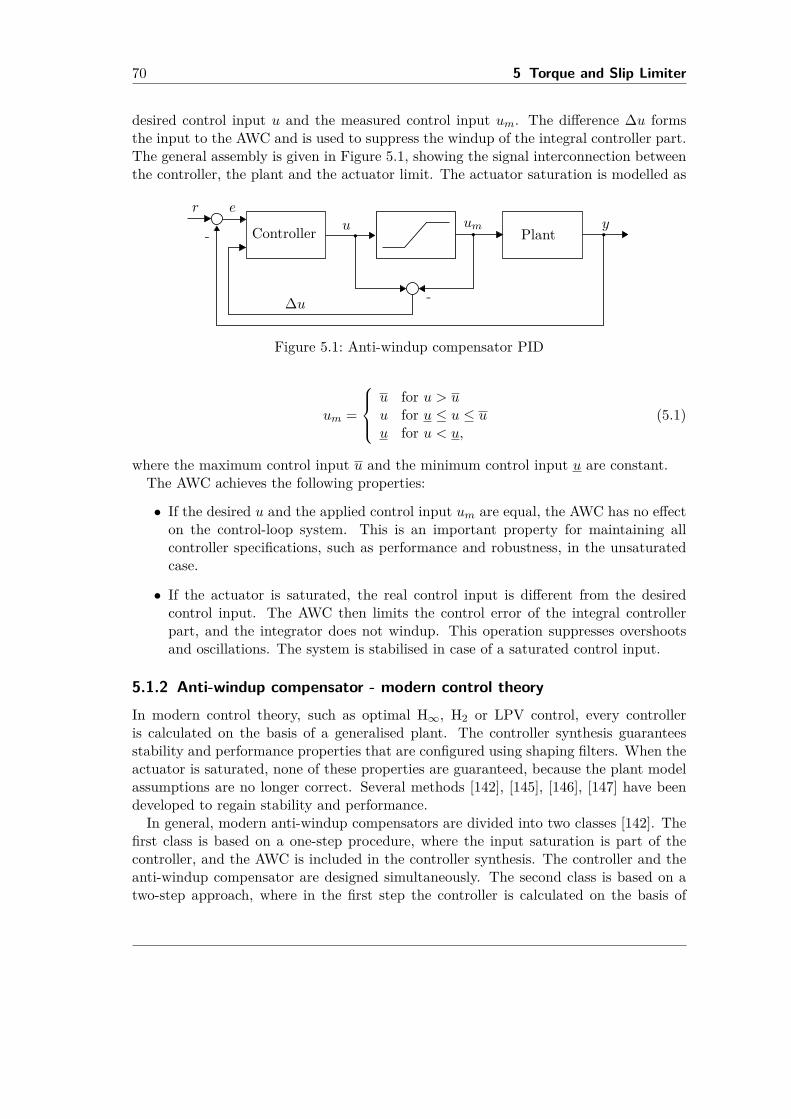
70 5 Torque and Slip Limiter
desired control input u and the measured control input um. The difference ∆u formsthe input to the AWC and is used to suppress the windup of the integral controller part.The general assembly is given in Figure 5.1, showing the signal interconnection betweenthe controller, the plant and the actuator limit. The actuator saturation is modelled as
Controller Plantumu
∆u
yr e
-
-
Figure 5.1: Anti-windup compensator PID
um =
u for u > uu for u ≤ u ≤ uu for u < u,
(5.1)
where the maximum control input u and the minimum control input u are constant.The AWC achieves the following properties:
• If the desired u and the applied control input um are equal, the AWC has no effecton the control-loop system. This is an important property for maintaining allcontroller specifications, such as performance and robustness, in the unsaturatedcase.
• If the actuator is saturated, the real control input is different from the desiredcontrol input. The AWC then limits the control error of the integral controllerpart, and the integrator does not windup. This operation suppresses overshootsand oscillations. The system is stabilised in case of a saturated control input.
5.1.2 Anti-windup compensator - modern control theoryIn modern control theory, such as optimal H∞, H2 or LPV control, every controlleris calculated on the basis of a generalised plant. The controller synthesis guaranteesstability and performance properties that are configured using shaping filters. When theactuator is saturated, none of these properties are guaranteed, because the plant modelassumptions are no longer correct. Several methods [142], [145], [146], [147] have beendeveloped to regain stability and performance.In general, modern anti-windup compensators are divided into two classes [142]. The
first class is based on a one-step procedure, where the input saturation is part of thecontroller, and the AWC is included in the controller synthesis. The controller and theanti-windup compensator are designed simultaneously. The second class is based on atwo-step approach, where in the first step the controller is calculated on the basis of
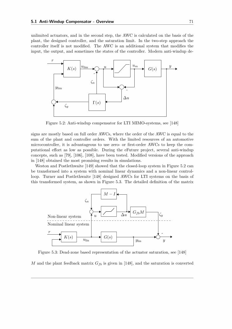
5.1 Anti-Windup Compensator - Overview 71
unlimited actuators, and in the second step, the AWC is calculated on the basis of theplant, the designed controller, and the saturation limit. In the two-step approach thecontroller itself is not modified. The AWC is an additional system that modifies theinput, the output, and sometimes the states of the controller. Modern anti-windup de-
r
ylim
ζu
ζy
∆u
u um yG(s)K(s)
Γ(s)
ulim
-
-
Figure 5.2: Anti-windup compensator for LTI MIMO-systems, see [148]
signs are mostly based on full order AWCs, where the order of the AWC is equal to thesum of the plant and controller orders. With the limited resources of an automotivemicrocontroller, it is advantageous to use zero- or first-order AWCs to keep the com-putational effort as low as possible. During the eFuture project, several anti-windupconcepts, such as [79], [106], [108], have been tested. Modified versions of the approachin [148] obtained the most promising results in simulations.Weston and Postlethwaite [149] showed that the closed-loop system in Figure 5.2 can
be transformed into a system with nominal linear dynamics and a non-linear control-loop. Turner and Postlethwaite [148] designed AWCs for LTI systems on the basis ofthis transformed system, as shown in Figure 5.3. The detailed definition of the matrix
Nominal linear system
K(s) G(s)
GfbM
M − Iζu
u ∆u ζy
yylin
Non-linear system
r
ulin
-
Figure 5.3: Dead-zone based representation of the actuator saturation, see [148]
M and the plant feedback matrix Gfb is given in [148], and the saturation is converted
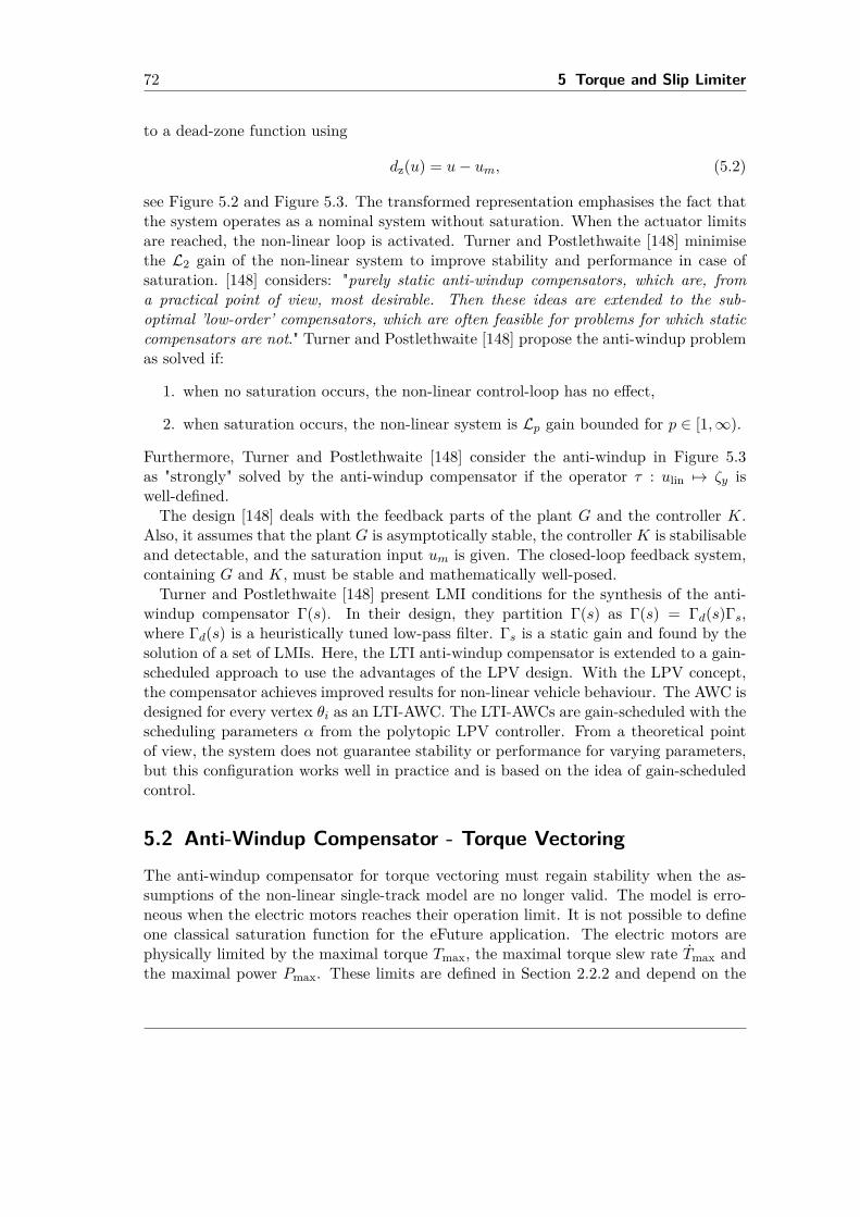
72 5 Torque and Slip Limiter
to a dead-zone function using
dz(u) = u− um, (5.2)
see Figure 5.2 and Figure 5.3. The transformed representation emphasises the fact thatthe system operates as a nominal system without saturation. When the actuator limitsare reached, the non-linear loop is activated. Turner and Postlethwaite [148] minimisethe L2 gain of the non-linear system to improve stability and performance in case ofsaturation. [148] considers: "purely static anti-windup compensators, which are, froma practical point of view, most desirable. Then these ideas are extended to the sub-optimal ’low-order’ compensators, which are often feasible for problems for which staticcompensators are not." Turner and Postlethwaite [148] propose the anti-windup problemas solved if:
1. when no saturation occurs, the non-linear control-loop has no effect,
2. when saturation occurs, the non-linear system is Lp gain bounded for p ∈ [1,∞).
Furthermore, Turner and Postlethwaite [148] consider the anti-windup in Figure 5.3as "strongly" solved by the anti-windup compensator if the operator τ : ulin 7→ ζy iswell-defined.The design [148] deals with the feedback parts of the plant G and the controller K.
Also, it assumes that the plant G is asymptotically stable, the controller K is stabilisableand detectable, and the saturation input um is given. The closed-loop feedback system,containing G and K, must be stable and mathematically well-posed.Turner and Postlethwaite [148] present LMI conditions for the synthesis of the anti-
windup compensator Γ(s). In their design, they partition Γ(s) as Γ(s) = Γd(s)Γs,where Γd(s) is a heuristically tuned low-pass filter. Γs is a static gain and found by thesolution of a set of LMIs. Here, the LTI anti-windup compensator is extended to a gain-scheduled approach to use the advantages of the LPV design. With the LPV concept,the compensator achieves improved results for non-linear vehicle behaviour. The AWC isdesigned for every vertex θi as an LTI-AWC. The LTI-AWCs are gain-scheduled with thescheduling parameters α from the polytopic LPV controller. From a theoretical pointof view, the system does not guarantee stability or performance for varying parameters,but this configuration works well in practice and is based on the idea of gain-scheduledcontrol.
5.2 Anti-Windup Compensator - Torque VectoringThe anti-windup compensator for torque vectoring must regain stability when the as-sumptions of the non-linear single-track model are no longer valid. The model is erro-neous when the electric motors reaches their operation limit. It is not possible to defineone classical saturation function for the eFuture application. The electric motors arephysically limited by the maximal torque Tmax, the maximal torque slew rate Tmax andthe maximal power Pmax. These limits are defined in Section 2.2.2 and depend on the
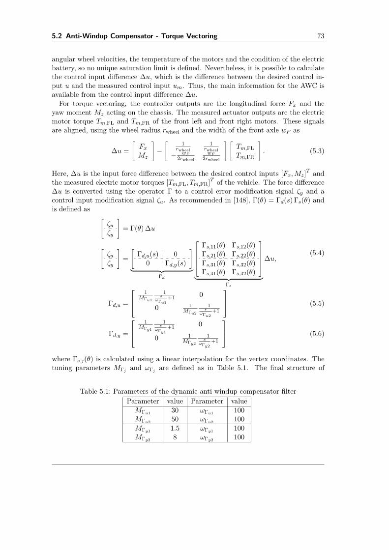
5.2 Anti-Windup Compensator - Torque Vectoring 73
angular wheel velocities, the temperature of the motors and the condition of the electricbattery, so no unique saturation limit is defined. Nevertheless, it is possible to calculatethe control input difference ∆u, which is the difference between the desired control in-put u and the measured control input um. Thus, the main information for the AWC isavailable from the control input difference ∆u.For torque vectoring, the controller outputs are the longitudinal force Fx and the
yaw moment Mz acting on the chassis. The measured actuator outputs are the electricmotor torque Tm,FL and Tm,FR of the front left and front right motors. These signalsare aligned, using the wheel radius rwheel and the width of the front axle wF as
∆u =[FxMz
]−[ 1
rwheel1
rwheel− wF
2rwheelwF
2rwheel
] [Tm,FLTm,FR
]. (5.3)
Here, ∆u is the input force difference between the desired control inputs [Fx,Mz]T andthe measured electric motor torques [Tm,FL, Tm,FR]T of the vehicle. The force difference∆u is converted using the operator Γ to a control error modification signal ζy and acontrol input modification signal ζu. As recommended in [148], Γ(θ) = Γd(s) Γs(θ) andis defined as [
ζuζy
]= Γ(θ) ∆u
[ζuζy
]=[
Γd,u(s) 00 Γd,y(s)
]︸ ︷︷ ︸
Γd
Γs,11(θ) Γs,12(θ)Γs,21(θ) Γs,22(θ)Γs,31(θ) Γs,32(θ)Γs,41(θ) Γs,42(θ)
︸ ︷︷ ︸
Γs
∆u,(5.4)
Γd,u =
1MΓu1
1s
ωΓu1+1 0
0 1MΓu2
1s
ωΓu2+1
(5.5)
Γd,y =
1
MΓy1
1s
ωΓy1+1 0
0 1MΓy2
1s
ωΓy2+1
(5.6)
where Γs,j(θ) is calculated using a linear interpolation for the vertex coordinates. Thetuning parameters MΓj and ωΓj are defined as in Table 5.1. The final structure of
Table 5.1: Parameters of the dynamic anti-windup compensator filterParameter value Parameter valueMΓu1 30 ωΓu1 100MΓu2 50 ωΓu2 100MΓy1 1.5 ωΓy1 100MΓy2 8 ωΓy2 100
74 5 Torque and Slip Limiter
the torque vectoring anti-windup compensator is given in Figure 5.4, where the generalclosed-loop system is extended using the AWC Γ and the controller modification signalsζu and ζy.
r e
ζy
K(θ) G(θ)
Γs(θ)Γd(s)
u
ζu
Γ
y
∆u
umeMot
-
--
Figure 5.4: Structure of the AWC for electric motor saturation
5.3 Wheel Slip Limitation
Simulations and virtual driving tests with the driving simulator [150] showed improvedvehicle behaviour due to use of the anti-windup compensator. Strong acceleration, brak-ing or steering requests are no longer problematic. However, the torque vectoring con-troller shows unsatisfying results for "bad" road conditions, like icy roads or very wetroads. Acceleration is not optimal. The lateral performance of the vehicle is reducedand even unstable in certain cases.
5.3.1 Wheel slip limitation - standard applications
The unwanted vehicle behaviour is related to the excessive wheel slip of the front tyres.Wheel slip is necessary to generate longitudinal tyre forces but with increased longitudi-nal wheel slip, the potential lateral tyre forces are reduced. Reduced tyre forces lead tounstable lateral movement of the vehicle. As described in Section 3.1.1, this phenomenais well known and resolved in serial vehicles with systems like ABS and TCS. The mainidea of ABS is to limit the braking forces if the wheels slow down too much, and thewheel slippage (or the angular acceleration of the wheels) exceeds defined thresholds. Inprinciple, TCS operates like ABS, but TCS limits excessive accelerations of the wheelsby reducing the motor torques or employing the hydraulic brakes. Detailed explanationsare given by Bosch [35] and Isermann [151]. Nonetheless, standard ABS and TCS sys-tems have not been developed for electric vehicles and would need additional work toextend the systems for an electric drivetrain. In a standard automotive vehicle, thesefunctions are separated. Here, it is shown that these functions can be integrated into asingle torque vectoring controller.
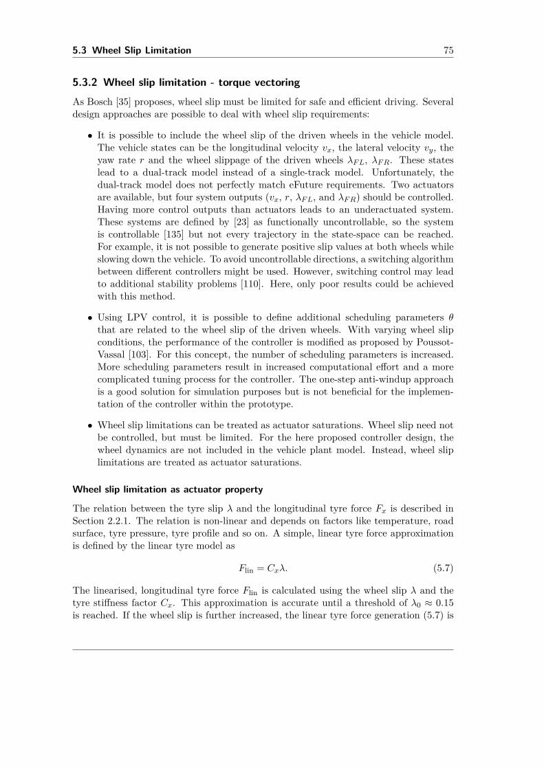
5.3 Wheel Slip Limitation 75
5.3.2 Wheel slip limitation - torque vectoring
As Bosch [35] proposes, wheel slip must be limited for safe and efficient driving. Severaldesign approaches are possible to deal with wheel slip requirements:
• It is possible to include the wheel slip of the driven wheels in the vehicle model.The vehicle states can be the longitudinal velocity vx, the lateral velocity vy, theyaw rate r and the wheel slippage of the driven wheels λFL, λFR. These stateslead to a dual-track model instead of a single-track model. Unfortunately, thedual-track model does not perfectly match eFuture requirements. Two actuatorsare available, but four system outputs (vx, r, λFL, and λFR) should be controlled.Having more control outputs than actuators leads to an underactuated system.These systems are defined by [23] as functionally uncontrollable, so the systemis controllable [135] but not every trajectory in the state-space can be reached.For example, it is not possible to generate positive slip values at both wheels whileslowing down the vehicle. To avoid uncontrollable directions, a switching algorithmbetween different controllers might be used. However, switching control may leadto additional stability problems [110]. Here, only poor results could be achievedwith this method.
• Using LPV control, it is possible to define additional scheduling parameters θthat are related to the wheel slip of the driven wheels. With varying wheel slipconditions, the performance of the controller is modified as proposed by Poussot-Vassal [103]. For this concept, the number of scheduling parameters is increased.More scheduling parameters result in increased computational effort and a morecomplicated tuning process for the controller. The one-step anti-windup approachis a good solution for simulation purposes but is not beneficial for the implemen-tation of the controller within the prototype.
• Wheel slip limitations can be treated as actuator saturations. Wheel slip need notbe controlled, but must be limited. For the here proposed controller design, thewheel dynamics are not included in the vehicle plant model. Instead, wheel sliplimitations are treated as actuator saturations.
Wheel slip limitation as actuator property
The relation between the tyre slip λ and the longitudinal tyre force Fx is described inSection 2.2.1. The relation is non-linear and depends on factors like temperature, roadsurface, tyre pressure, tyre profile and so on. A simple, linear tyre force approximationis defined by the linear tyre model as
Flin = Cxλ. (5.7)
The linearised, longitudinal tyre force Flin is calculated using the wheel slip λ and thetyre stiffness factor Cx. This approximation is accurate until a threshold of λ0 ≈ 0.15is reached. If the wheel slip is further increased, the linear tyre force generation (5.7) is
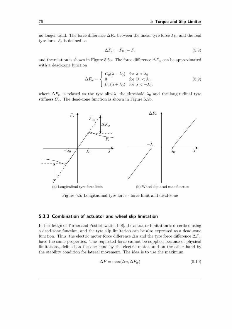
76 5 Torque and Slip Limiter
no longer valid. The force difference ∆Fw between the linear tyre force Flin and the realtyre force Fr is defined as
∆Fw = Flin − Fr (5.8)
and the relation is shown in Figure 5.5a. The force difference ∆Fw can be approximatedwith a dead-zone function
∆Fw =
Cx(λ− λ0) for λ > λ00 for |λ| < λ0Cx(λ+ λ0) for λ < −λ0,
(5.9)
where ∆Fw is related to the tyre slip λ, the threshold λ0 and the longitudinal tyrestiffness Cx. The dead-zone function is shown in Figure 5.5b.
Fx
λλ0
--−λ0
∆FwFlin
Fr
(a) Longitudinal tyre force limit
∆Fw
λλ0
--−λ0
(b) Wheel slip dead-zone function
Figure 5.5: Longitudinal tyre force - force limit and dead-zone
5.3.3 Combination of actuator and wheel slip limitation
In the design of Turner and Postlethwaite [148], the actuator limitation is described usinga dead-zone function, and the tyre slip limitation can be also expressed as a dead-zonefunction. Thus, the electric motor force difference ∆u and the tyre force difference ∆Fwhave the same properties. The requested force cannot be supplied because of physicallimitations, defined on the one hand by the electric motor, and on the other hand bythe stability condition for lateral movement. The idea is to use the maximum
∆F = max(∆u,∆Fw) (5.10)
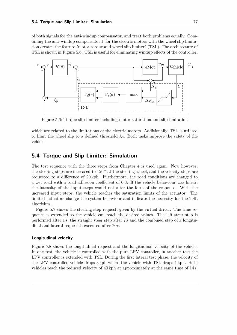
5.4 Torque and Slip Limiter: Simulation 77
of both signals for the anti-windup compensator, and treat both problems equally. Com-bining the anti-windup compensator Γ for the electric motors with the wheel slip limita-tion creates the feature "motor torque and wheel slip limiter" (TSL). The architecture ofTSL is shown in Figure 5.6. TSL is useful for eliminating windup effects of the controller,
r e
ζy
K(θ) Vehicle
Γs(θ)Γd(s)
u
ζu
y
∆u
umeMot
-
--
λ
∆Fwmax
TSL
Figure 5.6: Torque slip limiter including motor saturation and slip limitation
which are related to the limitations of the electric motors. Additionally, TSL is utilisedto limit the wheel slip to a defined threshold λ0. Both tasks improve the safety of thevehicle.
5.4 Torque and Slip Limiter: Simulation
The test sequence with the three steps from Chapter 4 is used again. Now however,the steering steps are increased to 120 at the steering wheel, and the velocity steps arerequested to a difference of 20 kph. Furthermore, the road conditions are changed toa wet road with a road adhesion coefficient of 0.3. If the vehicle behaviour was linear,the intensity of the input steps would not alter the form of the response. With theincreased input steps, the vehicle reaches the saturation limits of the actuator. Thelimited actuators change the system behaviour and indicate the necessity for the TSLalgorithm.Figure 5.7 shows the steering step request, given by the virtual driver. The time se-
quence is extended so the vehicle can reach the desired values. The left steer step isperformed after 1 s, the straight steer step after 7 s and the combined step of a longitu-dinal and lateral request is executed after 20 s.
Longitudinal velocity
Figure 5.8 shows the longitudinal request and the longitudinal velocity of the vehicle.In one test, the vehicle is controlled with the pure LPV controller, in another test theLPV controller is extended with TSL. During the first lateral test phase, the velocity ofthe LPV controlled vehicle drops 3 kph where the vehicle with TSL drops 1 kph. Bothvehicles reach the reduced velocity of 40 kph at approximately at the same time of 14 s.
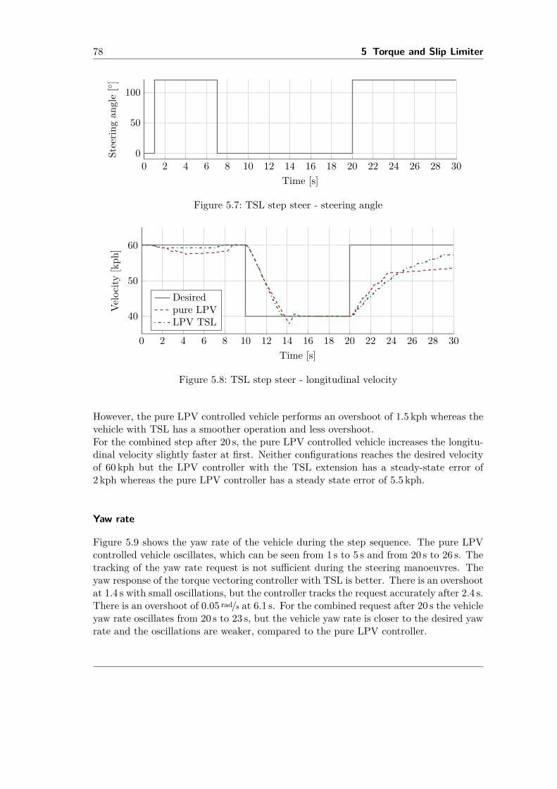
78 5 Torque and Slip Limiter
0 2 4 6 8 10 12 14 16 18 20 22 24 26 28 300
50
100
Time [s]
Stee
ring
angl
e[ ]
Figure 5.7: TSL step steer - steering angle
0 2 4 6 8 10 12 14 16 18 20 22 24 26 28 30
40
50
60
Time [s]
Velo
city
[kph
]
Desiredpure LPVLPV TSL
Figure 5.8: TSL step steer - longitudinal velocity
However, the pure LPV controlled vehicle performs an overshoot of 1.5 kph whereas thevehicle with TSL has a smoother operation and less overshoot.For the combined step after 20 s, the pure LPV controlled vehicle increases the longitu-dinal velocity slightly faster at first. Neither configurations reaches the desired velocityof 60 kph but the LPV controller with the TSL extension has a steady-state error of2 kph whereas the pure LPV controller has a steady state error of 5.5 kph.
Yaw rate
Figure 5.9 shows the yaw rate of the vehicle during the step sequence. The pure LPVcontrolled vehicle oscillates, which can be seen from 1 s to 5 s and from 20 s to 26 s. Thetracking of the yaw rate request is not sufficient during the steering manoeuvres. Theyaw response of the torque vectoring controller with TSL is better. There is an overshootat 1.4 s with small oscillations, but the controller tracks the request accurately after 2.4 s.There is an overshoot of 0.05 rad/s at 6.1 s. For the combined request after 20 s the vehicleyaw rate oscillates from 20 s to 23 s, but the vehicle yaw rate is closer to the desired yawrate and the oscillations are weaker, compared to the pure LPV controller.
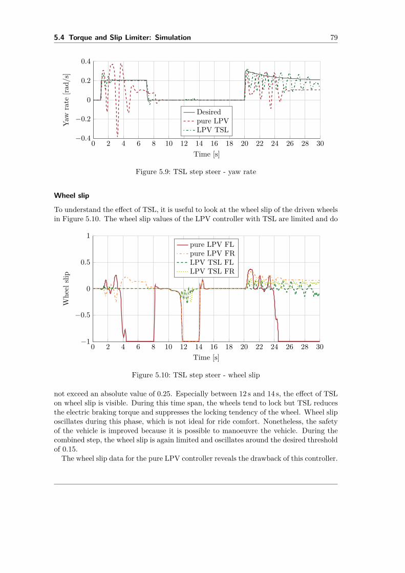
5.4 Torque and Slip Limiter: Simulation 79
0 2 4 6 8 10 12 14 16 18 20 22 24 26 28 30−0.4
−0.2
0
0.2
0.4
Time [s]
Yaw
rate
[rad/
s]
Desiredpure LPVLPV TSL
Figure 5.9: TSL step steer - yaw rate
Wheel slip
To understand the effect of TSL, it is useful to look at the wheel slip of the driven wheelsin Figure 5.10. The wheel slip values of the LPV controller with TSL are limited and do
0 2 4 6 8 10 12 14 16 18 20 22 24 26 28 30−1
−0.5
0
0.5
1
Time [s]
Whe
elsli
p
pure LPV FLpure LPV FRLPV TSL FLLPV TSL FR
Figure 5.10: TSL step steer - wheel slip
not exceed an absolute value of 0.25. Especially between 12 s and 14 s, the effect of TSLon wheel slip is visible. During this time span, the wheels tend to lock but TSL reducesthe electric braking torque and suppresses the locking tendency of the wheel. Wheel sliposcillates during this phase, which is not ideal for ride comfort. Nonetheless, the safetyof the vehicle is improved because it is possible to manoeuvre the vehicle. During thecombined step, the wheel slip is again limited and oscillates around the desired thresholdof 0.15.The wheel slip data for the pure LPV controller reveals the drawback of this controller.
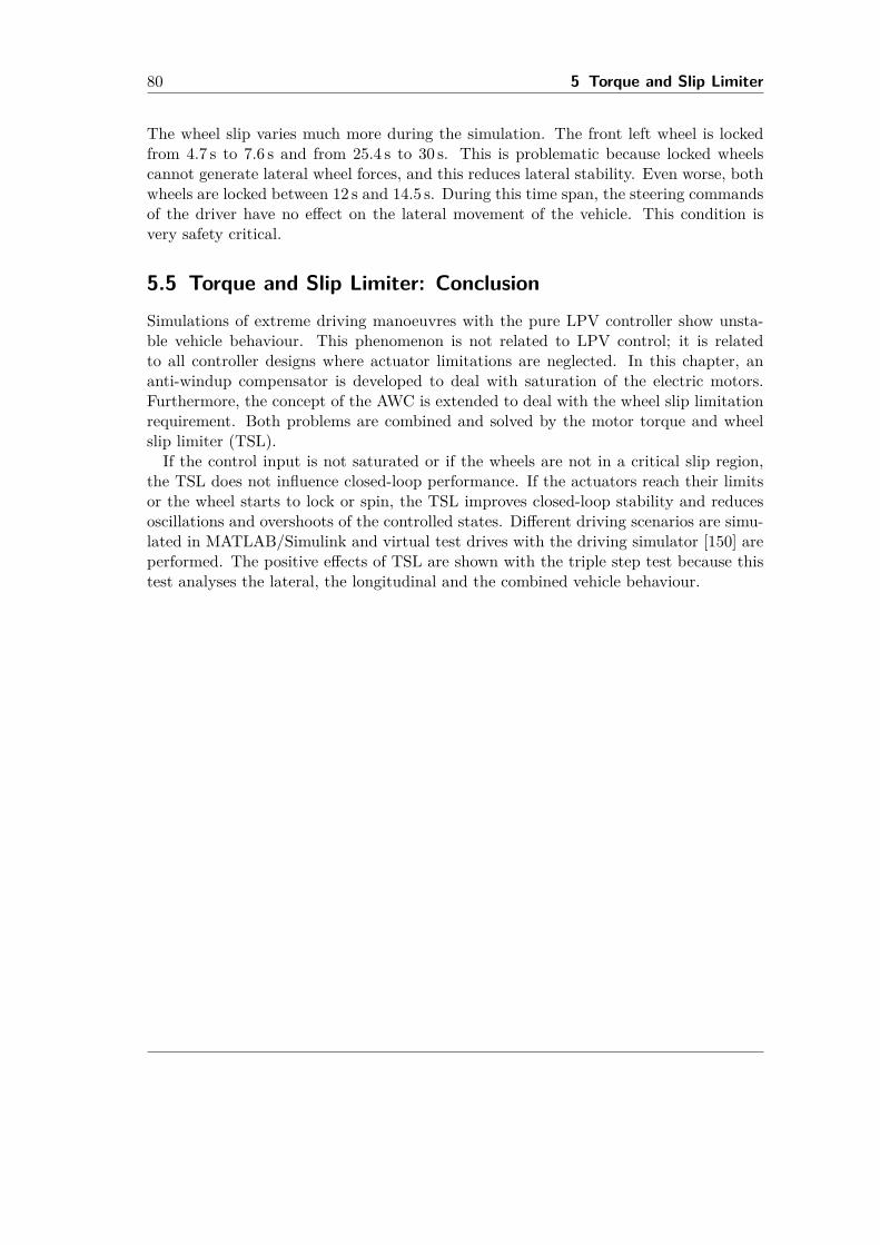
80 5 Torque and Slip Limiter
The wheel slip varies much more during the simulation. The front left wheel is lockedfrom 4.7 s to 7.6 s and from 25.4 s to 30 s. This is problematic because locked wheelscannot generate lateral wheel forces, and this reduces lateral stability. Even worse, bothwheels are locked between 12 s and 14.5 s. During this time span, the steering commandsof the driver have no effect on the lateral movement of the vehicle. This condition isvery safety critical.
5.5 Torque and Slip Limiter: ConclusionSimulations of extreme driving manoeuvres with the pure LPV controller show unsta-ble vehicle behaviour. This phenomenon is not related to LPV control; it is relatedto all controller designs where actuator limitations are neglected. In this chapter, ananti-windup compensator is developed to deal with saturation of the electric motors.Furthermore, the concept of the AWC is extended to deal with the wheel slip limitationrequirement. Both problems are combined and solved by the motor torque and wheelslip limiter (TSL).If the control input is not saturated or if the wheels are not in a critical slip region,
the TSL does not influence closed-loop performance. If the actuators reach their limitsor the wheel starts to lock or spin, the TSL improves closed-loop stability and reducesoscillations and overshoots of the controlled states. Different driving scenarios are simu-lated in MATLAB/Simulink and virtual test drives with the driving simulator [150] areperformed. The positive effects of TSL are shown with the triple step test because thistest analyses the lateral, the longitudinal and the combined vehicle behaviour.
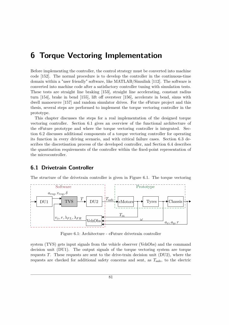
6 Torque Vectoring Implementation
Before implementing the controller, the control strategy must be converted into machinecode [152]. The normal procedure is to develop the controller in the continuous-timedomain within a "user friendly" software, like MATLAB/Simulink [112]. The software isconverted into machine code after a satisfactory controller tuning with simulation tests.These tests are straight line braking [153], straight line accelerating, constant radiusturn [154], brake in bend [155], lift off oversteer [156], accelerate in bend, sinus withdwell manoeuvre [157] and random simulator drives. For the eFuture project and thisthesis, several steps are performed to implement the torque vectoring controller in theprototype.This chapter discusses the steps for a real implementation of the designed torque
vectoring controller. Section 6.1 gives an overview of the functional architecture ofthe eFuture prototype and where the torque vectoring controller is integrated. Sec-tion 6.2 discusses additional components of a torque vectoring controller for operatingits function in every driving scenario, and with critical failure cases. Section 6.3 de-scribes the discretisation process of the developed controller, and Section 6.4 describesthe quantisation requirements of the controller within the fixed-point representation ofthe microcontroller.
6.1 Drivetrain ControllerThe structure of the drivetrain controller is given in Figure 6.1. The torque vectoring
DU1 TVS eMotors Tyres ChassisDU2
VehObs
T Tsafe
Tmω
ax, ay, rvx, r, λFL, λFR
areq, vreq, δ
PrototypeSoftware
Figure 6.1: Architecture - eFuture drivetrain controller
system (TVS) gets input signals from the vehicle observer (VehObs) and the commanddecision unit (DU1). The output signals of the torque vectoring system are torquerequests T . These requests are sent to the drive-train decision unit (DU2), where therequests are checked for additional safety concerns and sent, as Tsafe, to the electric
81
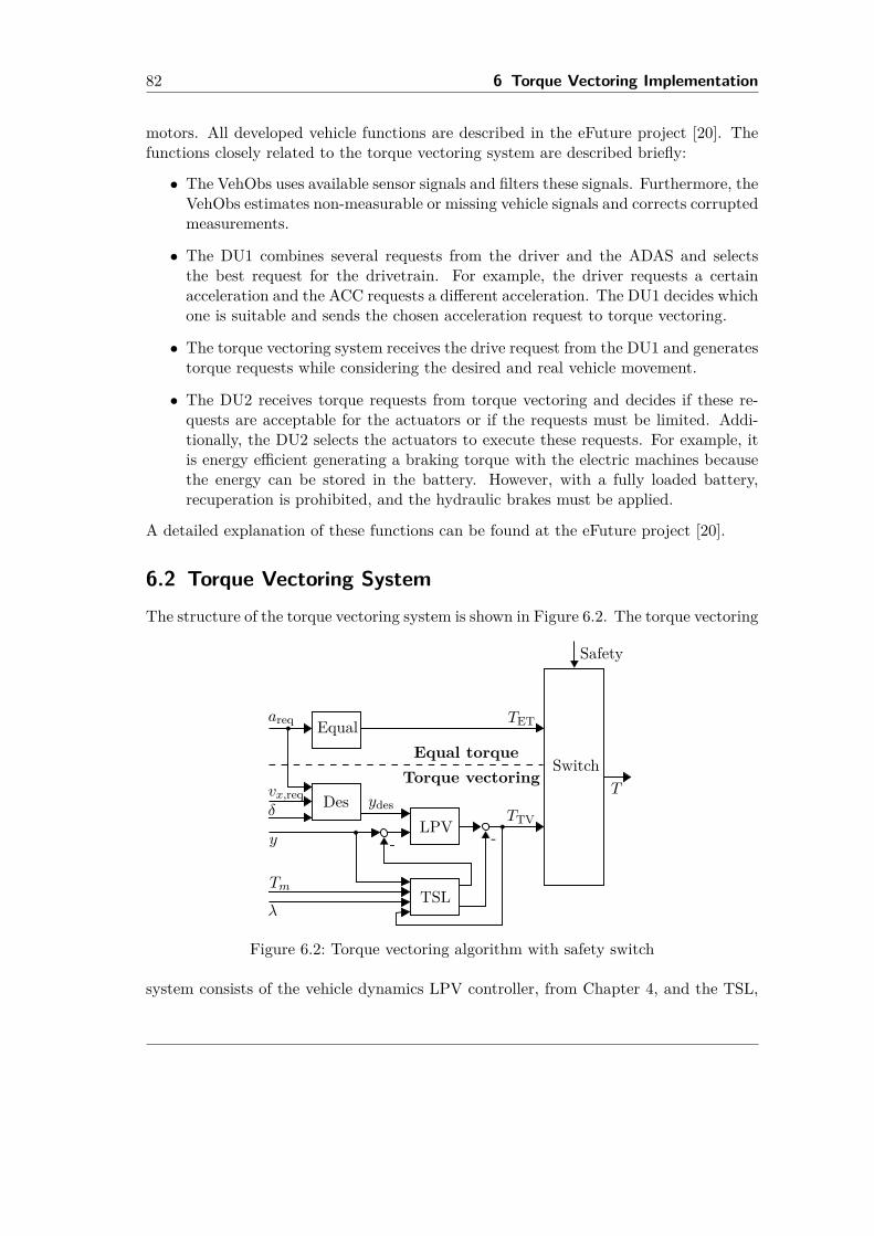
82 6 Torque Vectoring Implementation
motors. All developed vehicle functions are described in the eFuture project [20]. Thefunctions closely related to the torque vectoring system are described briefly:
• The VehObs uses available sensor signals and filters these signals. Furthermore, theVehObs estimates non-measurable or missing vehicle signals and corrects corruptedmeasurements.
• The DU1 combines several requests from the driver and the ADAS and selectsthe best request for the drivetrain. For example, the driver requests a certainacceleration and the ACC requests a different acceleration. The DU1 decides whichone is suitable and sends the chosen acceleration request to torque vectoring.
• The torque vectoring system receives the drive request from the DU1 and generatestorque requests while considering the desired and real vehicle movement.
• The DU2 receives torque requests from torque vectoring and decides if these re-quests are acceptable for the actuators or if the requests must be limited. Addi-tionally, the DU2 selects the actuators to execute these requests. For example, itis energy efficient generating a braking torque with the electric machines becausethe energy can be stored in the battery. However, with a fully loaded battery,recuperation is prohibited, and the hydraulic brakes must be applied.
A detailed explanation of these functions can be found at the eFuture project [20].
6.2 Torque Vectoring SystemThe structure of the torque vectoring system is shown in Figure 6.2. The torque vectoring
Equal
LPVDes
TSL
Safety
SwitchT
TET
TTVydes
-y
areq
vx,req
Tm
δ
λ
Equal torqueTorque vectoring
-
Figure 6.2: Torque vectoring algorithm with safety switch
system consists of the vehicle dynamics LPV controller, from Chapter 4, and the TSL,
6.2 Torque Vectoring System 83
from Chapter 5. Additional constraints are considered for implementing the torquevectoring system in a real vehicle. The LPV controller design is based on the STM(2.13)-(2.15). This model is not adequate for reverse driving, and the model is notnumerically defined for standstill. Additionally, the lateral moment Mz has no positiveeffect for low velocities and does not improve the control of the vehicle. If the LPVcontroller cannot be used, the equal torque (ET) controller is activated.
6.2.1 Equal torque distributionThe basic idea of equal torque distribution is to copy the mechanical differential [158],[159] of a standard drivetrain. Within a differential, the torque of the combustion engineis equally split to the driven wheels. Two independently controlled motors are integratedin the eFuture prototype, so no mechanical differential is necessary. However, the soft-ware component ET emulates a mechanical differential. Within the ET, the accelerationrequest is multiplied with a constant gain CT and the resultant torque request is theoutput. The gain CT is defined as
CT = mR
2 , (6.1)
wherem is the vehicle mass andR the effective tyre radius. As with a classical mechanicaldifferential, no torque distribution and no control laws are introduced.
6.2.2 Torque vectoring activationThe proposed torque distribution algorithm is activated above 18 kph and deactivatedbelow 15 kph. A time dependent, linear interpolation is implemented for the transi-tion between torque vectoring and equal torque distribution. The smooth transitionsuppresses discontinuous torque requests that would lead to an uncomfortable vehicleoperation. During linear interpolation, the stability of the system is not guaranteed. Nounstable situation has yet been caused by the linear interpolated switching.Besides longitudinal vehicle velocity, several other factors may disable the torque vec-
toring controller. Safety checks are defined in the eFuture project and documentedin [20]. Torque vectoring is deactivated if lateral vehicle control with the electric ma-chines may be unreasonable. For example, if the yaw rate sensor is inoperable, no torquedistribution is allowed, and the driver is informed about the malfunction of the vehicle.If the error is more severe, the torque request is set to 0Nm. This occurs if the tem-perature of the battery exceeds the critical thermal limit. Finally, the torque vectoringfunction has three general states:
1. The torque request is set to 0Nm if a serious error occurs and driving is inhibited.
2. Equal torque distribution is used if uncritical errors occur or if the vehicle drivesslowly in reverse.
3. Torque distribution is activated if the vehicle drives faster than 18 kph and no erroris detected.
84 6 Torque Vectoring Implementation
6.2.3 Desired value generator
The desired value generator (DVG) is used to convert the steering request and theacceleration or velocity request from DU1 into a velocity request and a yaw rate request.
Longitudinal request
The longitudinal request is sent by DU1 as a velocity request vreq or an accelerationrequest areq. Additionally, the status of both signals is sent to determine which requestshould be taken. If the velocity request should be accepted, the DU1 velocity requestis routed to the LPV controller. If the acceleration request should be accepted, theacceleration request is converted to a virtual velocity request using
vreq = vmeas + f · areq, (6.2)
where f is a tuning factor and vmeas the measured velocity of the vehicle.
Lateral request
For the conversion from steering request to yaw rate request, several transformations arepossible:
• The simplest conversion is a non-linear gain operation [34], [74], [80], [85], [90], [96]or a lookup-table [81], [82]. Using static gains neglects the dynamic time responseof the vehicle, which is physically generated between the steering angle changesand the yaw rate changes. Ignoring the time delay leads to overshoots in theclosed-loop behaviour for yaw control.
• Another strategy is to use a non-linear gain and a first-order filter [46], [72], [78] ora second-order filter [44], [100] for the vehicle dynamics. These methods require anexcessive tuning process and do not provide information about the desired lateralvelocity.
• The third method uses a linear single-track model to generate the desired yawrate. The input signals are the steering wheel angle and the vehicle velocity. Thisstrategy is used by [73], [86], [87], [88], [103]. The desired lateral motion of thevehicle is tuned using physical properties like vehicle mass or cornering stiffness,which are known for different vehicles. For example, the desired vehicle behaviourcan be designed for the properties of a small sports car or a comfortable van evenif the vehicle does not change its physical properties.
Here, the single-track model method is used for the DVG. The function is tuned toemulate an automobile that is 12% lighter with a 16.5% lower front cornering stiffness.The emulated vehicle understeers less and reacts faster to steering inputs. The desired
6.3 Discrete-Time LPV Controller Design 85
vehicle dynamics are defined as
˙β = − Cy,F + Cy,R
mvx,mβ +
(−lF Cy,F + lRCy,R
mv2x,m
− 1)r + Cy,F
mvx,mδm (6.3)
˙r = −lF Cy,F + lRCy,R
Izβ − l2F Cy,F + l2RCy,R
Izvx,mr + lF Cy,F
Izδm. (6.4)
The desired distance from the front axle to the CoG is lF , and the desired distance fromthe CoG to the rear axle is lR. The desired cornering stiffness for the front axle Cy,F ,and the rear axle Cy,R, the desired vehicle mass m and the desired moment of inertiaIz are chosen by the function designer. The desired sideslip angle β and the desiredyaw rate r are calculated using (6.3, 6.4), given the measured steering angle δm and themeasured longitudinal velocity vx,m.Remark 6.1 The sideslip angle is used to describe the desired vehicle behaviour, ratherthan the lateral velocity . Both states are interchangeable, but it is easier to comparedifferent vehicle manoeuvres (with varying longitudinal velocities) if the sideslip angle isused.Several studies ( [32], [73], [160]) recommend limiting the vehicle states to request acontrollable vehicle movement without excessive tyre saturation. Therefore, the desiredvehicle states are limited using
|r| < sMµg
vx,meas(6.5)
|β| < tan−1(0.02µg), (6.6)
where µ defines the maximum road adhesion coefficient and g the Earth’s gravity. Ra-jamani [160] recommends a safety margin sM between 0.85 and 1.5 for (6.5). Followingreal test drives, the safety margin sM is set empirically to the value of 1.27.
6.3 Discrete-Time LPV Controller DesignThe behaviour of physical systems is precisely described using differential equations incontinuous-time representation because most physical systems operate continuously. Forexample, a vehicle moves in space in continuous-time and does not perform discontinuousmovements. Physical equations are developed to describe this behaviour. By contrast,most controllers for regulating physical systems are implemented on microcontrollersthat operate in the discrete-time domain. There are two different approaches to dealwith the different representations of the time domain:
• Convert the physical continuous-time model of the system into a discrete-timemodel and calculate a discrete-time controller based on the discrete-time plantmodel.
• Calculate a continuous-time controller for the continuous-time plant model and
86 6 Torque Vectoring Implementation
convert the continuous-time controller into a discrete-time controller. This dis-cretisation process is called emulation.
A rule of thumb for LTI systems with single input / single output behaviour is thatcontinuous-time controller synthesis can be used if the bandwidth of the microcontrolleris about 20-30 times higher [161], [162] than the bandwidth of the system. For thediscrete-time controller synthesis, the bandwidth of the controller should be at least 4-10 times higher [161], [162] [163] than the bandwidth of the system. No general rule ofthumb is yet available for discrete-time LPV controller designs. Toth et al. [164], [165]reported some interesting results. The present study uses knowledge of LTI systemsheuristically extended to discrete-time control of LPV systems. The LPV system islinearised at certain operation points and the maximum bandwidth of the system iscalculated. The ratio of the sampling bandwidth to the system bandwidth is calculatedfor these points and compared with known discretisation rules.• In the eFuture project [20], the sampling time TS of the microcontroller is limitedto 0.01 s. This results in a sampling frequency ωS of 628 rad/s using
ωS = 2πTS. (6.7)
• Linearised single-track models, from Section 3.4, are used to estimate the band-width of LTI models in the scheduling space. This step is performed for severaloperating points inside the polytope P. The -3 db cut-off frequency ωC [166] iscalculated using
ωC = 2|σP |, (6.8)
where σP represents the real part of the complex pole. Poles close to the origin areresponsible for low bandwidths, poles far in the LHP generate higher bandwidth.These far LHP poles are therefore called fast poles. These fast poles of the systemmust be considered for the bandwidth analysis.
• Dividing the sampling frequency ωS by the highest bandwidth ωC results in thesampling factor Fsample.
Fsample = ωSωC
. (6.9)
The factor Fsample is calculated for the vehicle model that is linearised in certainoperation points. The results are linearly interpolated and shown in Figure 6.3 aslevel curves.
As discussed, the sampling factor Fsample should be at least 4 for the discrete-timecontroller synthesis and at least 20 for the emulation process. The abscissa of Figure6.3 is the inverse scheduling signal 1/θ1, which results in a simplified representation. Itis observable that the sampling factor Fsample depends more on the longitudinal velocityand less on the yaw rate of the vehicle.
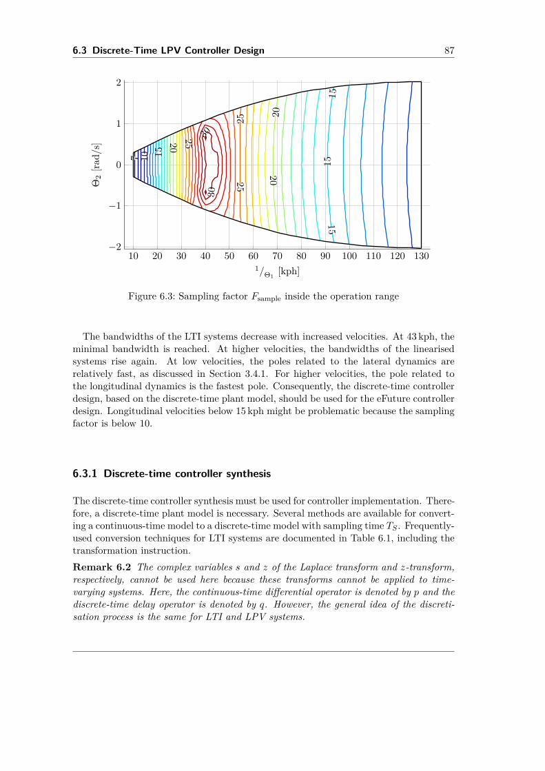
6.3 Discrete-Time LPV Controller Design 87
10 20 30 40 50 60 70 80 90 100 110 120 130−2
−1
0
1
2
7 10
15
1515
15
2020
20
25
25
25
3030
1/Θ1[kph]
Θ2
[rad/
s]
Figure 6.3: Sampling factor Fsample inside the operation range
The bandwidths of the LTI systems decrease with increased velocities. At 43 kph, theminimal bandwidth is reached. At higher velocities, the bandwidths of the linearisedsystems rise again. At low velocities, the poles related to the lateral dynamics arerelatively fast, as discussed in Section 3.4.1. For higher velocities, the pole related tothe longitudinal dynamics is the fastest pole. Consequently, the discrete-time controllerdesign, based on the discrete-time plant model, should be used for the eFuture controllerdesign. Longitudinal velocities below 15 kph might be problematic because the samplingfactor is below 10.
6.3.1 Discrete-time controller synthesis
The discrete-time controller synthesis must be used for controller implementation. There-fore, a discrete-time plant model is necessary. Several methods are available for convert-ing a continuous-time model to a discrete-time model with sampling time TS . Frequently-used conversion techniques for LTI systems are documented in Table 6.1, including thetransformation instruction.Remark 6.2 The complex variables s and z of the Laplace transform and z-transform,respectively, cannot be used here because these transforms cannot be applied to time-varying systems. Here, the continuous-time differential operator is denoted by p and thediscrete-time delay operator is denoted by q. However, the general idea of the discreti-sation process is the same for LTI and LPV systems.
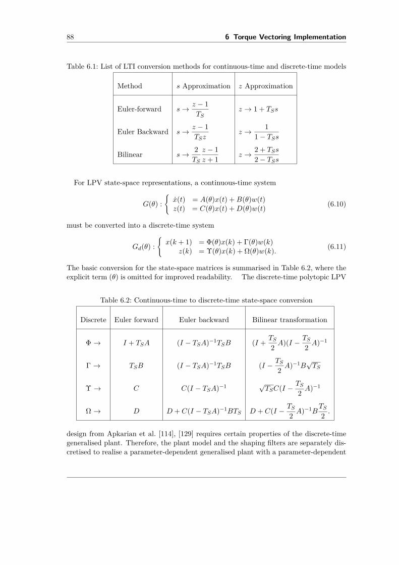
88 6 Torque Vectoring Implementation
Table 6.1: List of LTI conversion methods for continuous-time and discrete-time models
Method s Approximation z Approximation
Euler-forward s→ z − 1TS
z → 1 + TSs
Euler Backward s→ z − 1TSz
z → 11− TSs
Bilinear s→ 2TS
z − 1z + 1 z → 2 + TSs
2− TSs
For LPV state-space representations, a continuous-time system
G(θ) :x(t) = A(θ)x(t) +B(θ)w(t)z(t) = C(θ)x(t) +D(θ)w(t) (6.10)
must be converted into a discrete-time system
Gd(θ) :x(k + 1) = Φ(θ)x(k) + Γ(θ)w(k)
z(k) = Υ(θ)x(k) + Ω(θ)w(k). (6.11)
The basic conversion for the state-space matrices is summarised in Table 6.2, where theexplicit term (θ) is omitted for improved readability. The discrete-time polytopic LPV
Table 6.2: Continuous-time to discrete-time state-space conversion
Discrete Euler forward Euler backward Bilinear transformation
Φ → I + TSA (I − TSA)−1TSB (I + TS2 A)(I − TS
2 A)−1
Γ → TSB (I − TSA)−1TSB (I − TS2 A)−1B
√TS
Υ → C C(I − TSA)−1 √TSC(I − TS
2 A)−1
Ω → D D + C(I − TSA)−1BTS D + C(I − TS2 A)−1B
TS2 .
design from Apkarian et al. [114], [129] requires certain properties of the discrete-timegeneralised plant. Therefore, the plant model and the shaping filters are separately dis-cretised to realise a parameter-dependent generalised plant with a parameter-dependent
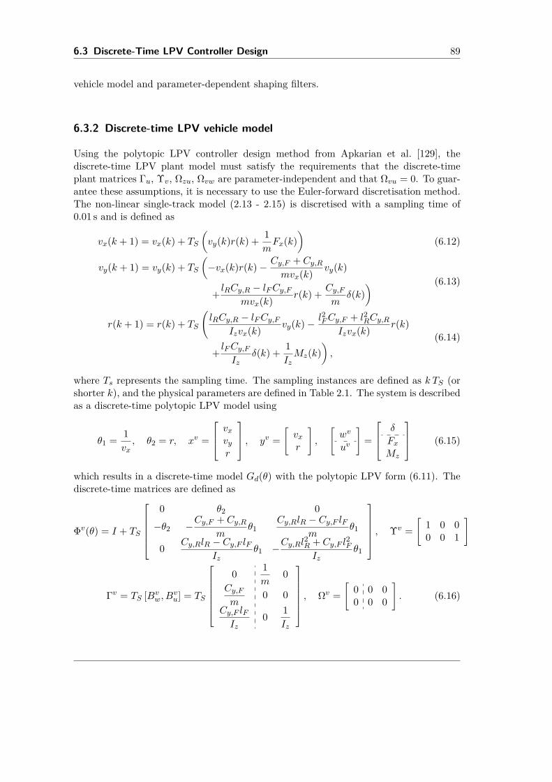
6.3 Discrete-Time LPV Controller Design 89
vehicle model and parameter-dependent shaping filters.
6.3.2 Discrete-time LPV vehicle model
Using the polytopic LPV controller design method from Apkarian et al. [129], thediscrete-time LPV plant model must satisfy the requirements that the discrete-timeplant matrices Γu, Υv, Ωzu, Ωvw are parameter-independent and that Ωvu = 0. To guar-antee these assumptions, it is necessary to use the Euler-forward discretisation method.The non-linear single-track model (2.13 - 2.15) is discretised with a sampling time of0.01 s and is defined as
vx(k + 1) = vx(k) + TS
(vy(k)r(k) + 1
mFx(k)
)(6.12)
vy(k + 1) = vy(k) + TS
(−vx(k)r(k)− Cy,F + Cy,R
mvx(k) vy(k)
+ lRCy,R − lFCy,Fmvx(k) r(k) + Cy,F
mδ(k)
) (6.13)
r(k + 1) = r(k) + TS
(lRCy,R − lFCy,F
Izvx(k) vy(k)− l2FCy,F + l2RCy,RIzvx(k) r(k)
+ lFCy,FIz
δ(k) + 1IzMz(k)
),
(6.14)
where Ts represents the sampling time. The sampling instances are defined as k TS (orshorter k), and the physical parameters are defined in Table 2.1. The system is describedas a discrete-time polytopic LPV model using
θ1 = 1vx, θ2 = r, xv =
vxvyr
, yv =[vxr
],
[wv
uv
]=
δ
FxMz
(6.15)
which results in a discrete-time model Gd(θ) with the polytopic LPV form (6.11). Thediscrete-time matrices are defined as
Φv(θ) = I + TS
0 θ2 0−θ2 −Cy,F + Cy,R
mθ1
Cy,RlR − Cy,F lFm
θ1
0 Cy,RlR − Cy,F lFIz
θ1 −Cy,Rl2R + Cy,F l
2F
Izθ1
, Υv =[
1 0 00 0 1
]
Γv = TS [Bvw, B
vu] = TS
0 1
m0
Cy,Fm
0 0Cy,F lFIz
0 1Iz
, Ωv =[
0 0 00 0 0
]. (6.16)
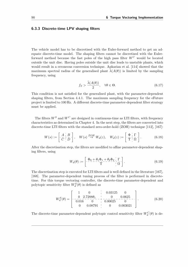
90 6 Torque Vectoring Implementation
6.3.3 Discrete-time LPV shaping filters
The vehicle model has to be discretised with the Euler-forward method to get an ad-equate discrete-time model. The shaping filters cannot be discretised with the Euler-forward method because the fast poles of the high pass filter WC would be locatedoutside the unit disc. Having poles outside the unit disc leads to unstable plants, whichwould result in a erroneous conversion technique. Apkarian et al. [114] showed that themaximum spectral radius of the generalised plant λ(A(θ)) is limited by the samplingfrequency, using
fS >λ(A(θ))
2 , ∀θ ∈ Θ. (6.17)
This condition is not satisfied for the generalised plant, with the parameter-dependentshaping filters, from Section 4.4.1. The maximum sampling frequency for the eFutureproject is limited to 100Hz. A different discrete-time parameter-dependent filter strategymust be applied.
The filters WS and WC are designed in continuous-time as LTI filters, with frequencycharacteristics as determined in Chapter 4. In the next step, the filters are converted intodiscrete-time LTI filters with the standard zero-order-hold (ZOH) technique [112], [167]:
W (s) :=[A B
C D
], W (s) ZOH→ Wd(z), Wd(z) :=
[Φ ΓΥ Ω
]. (6.18)
After the discretisation step, the filters are modified to affine parameter-dependent shap-ing filters, using
Wd(θ) :=[
Φ0 + θ1Φ1 + θ2Φ2 ΓΥ Ω
]. (6.19)
The discretisation step is executed for LTI filters and is well defined in the literature [167],[168]. The parameter-dependent tuning process of the filter is performed in discrete-time. For this torque vectoring controller, the discrete-time parameter-dependent andpolytopic sensitivity filter WS
d (θ) is defined as
WSd (θ) =
1 00 2.7288θ1
0.03125 00 0.0625
0.016 00 0.08791
0.00025 00 0.003021
. (6.20)
The discrete-time parameter-dependent polytopic control sensitivity filter WCd (θ) is de-
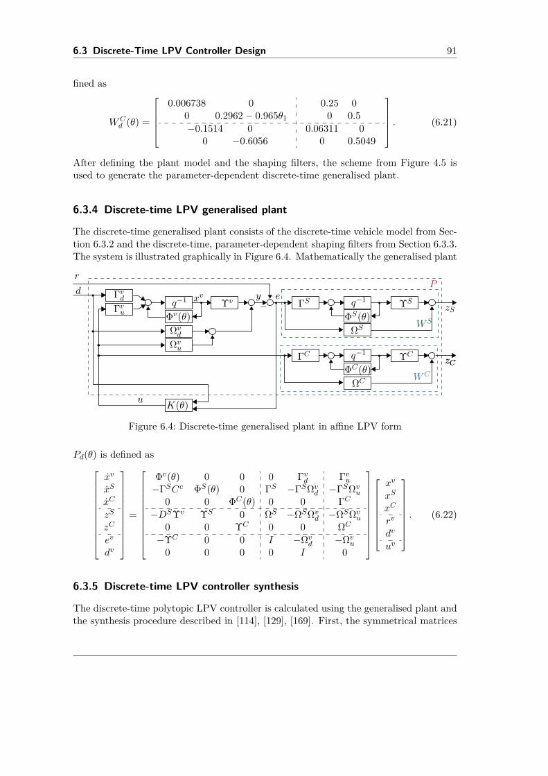
6.3 Discrete-Time LPV Controller Design 91
fined as
WCd (θ) =
0.006738 0
0 0.2962− 0.965θ1
0.25 00 0.5
−0.1514 00 −0.6056
0.06311 00 0.5049
. (6.21)
After defining the plant model and the shaping filters, the scheme from Figure 4.5 isused to generate the parameter-dependent discrete-time generalised plant.
6.3.4 Discrete-time LPV generalised plant
The discrete-time generalised plant consists of the discrete-time vehicle model from Sec-tion 6.3.2 and the discrete-time, parameter-dependent shaping filters from Section 6.3.3.The system is illustrated graphically in Figure 6.4. Mathematically the generalised plant
q−1 Υv
Φv(θ)Ωvd
Ωvu
y ezS
ΓvdΓvu
K(θ)
−d
r
xv
u
P
ΦS(θ)q−1ΓS ΥS
ΩS
zC
WS
WC
zCΦC(θ)q−1ΓC ΥC
ΩC
Figure 6.4: Discrete-time generalised plant in affine LPV form
Pd(θ) is defined as
xv
xS
xC
zS
zC
ev
dv
=
Φv(θ) 0 0 0 Γvd Γvu−ΓSCc ΦS(θ) 0 ΓS −ΓSΩv
d −ΓSΩvu
0 0 ΦC(θ) 0 0 ΓC−DSΥv ΥS 0 ΩS −ΩSΩv
d −ΩSΩvu
0 0 ΥC 0 0 ΩC
−ΥC 0 0 I −Ωvd −Ωv
u
0 0 0 0 I 0
xv
xS
xC
rv
dv
uv
. (6.22)
6.3.5 Discrete-time LPV controller synthesis
The discrete-time polytopic LPV controller is calculated using the generalised plant andthe synthesis procedure described in [114], [129], [169]. First, the symmetrical matrices
92 6 Torque Vectoring Implementation
Rd, Sd are found for the closed-loop system. The matrices Rd, Sd must satisfy LMIs
[NRdi 0
0 I
]T ΦiRdΦTi −Rd ΦiRdΥT
z,i Γw,i? −γI + Υz,iRdΥT
z,i Ωwz,i
? ? −γI
[ NRdi 00 I
]< 0 (6.23)
[NSdi 0
0 I
]T ΦTi SdΦi − Sd ΦT
i SdΓw,i ΥTz,i
? −γI + ΓTw,iSdΓw,i ΩTwz,i
? ? −γI
[ NSdi 00 I
]< 0 (6.24)
[Rd II Sd
]≥ 0, (6.25)
where NRdi and NSdi are the base of the null space from[Γu,i,ΩT
zu,i
]and
[Υv,i,ΩT
vw,i
].
Next, the Lyapunov matrix Xd,cl is defined as
MdNTd = I −RdSd (6.26)
Xd,cl =[Sd INTd 0
] [I Rd0 MT
d
]−1
. (6.27)
The discrete-time version of LMI conditions is defined as
Xd,cl = XTd,cl > 0 (6.28) ΦT
cl,iXd,clΦcl,i −Xd,cl ΦTcl,iXd,clΓcl,i ΥT
cl,i
? ΓTcl,iXd,clΓcl,i − I ΩTcl,i
? ? −I
< 0. (6.29)
The remaining procedure is similar to the continuous-time case, as described in Section4.1.1.
6.3.6 Discrete-time motor torque and wheel slip limiter
The motor torque and wheel slip limiter from Chapter 5 is calculated in discrete-timewith the discrete-time vehicle model from Section 6.3.2 and the discrete-time polytopicLPV controller from Section 6.3.5. The dynamic TSL is calculated as a low pass filterbut converted using ZOH operation into the discrete-time representation. As for thecontinuous-time case in Section 5, Turner et al. [170] propose a similar theorem fordiscrete-time, where operator τ maps the linear control input ulin to the non-linearcontrol output ζd as in Figure 5.3. By solving the proposed LMI [170] for all six vertices,the discrete-time LTI anti-windup compensators are calculated for every corner point.The resulting gains Ξi are linearly interpolated to deal with the non-linear single-trackmodel and the discrete-time polytopic LPV controller.
6.4 Quantisation of the Controller 93
6.4 Quantisation of the Controller
The eFuture project uses the microcontroller Freescale Bolero MPC5607B. The torquevectoring function is calculated using a sampling time of 0.01 s. In addition, five majorfunctions must be calculated by the same microcontroller. The automotive softwarestandard AUTOSAR [21] must be used for this project, which creates additional over-head for the base software calculation. The final requirement for the execution timeof the torque vectoring is that the compiled machine code must run within 1ms on themicrocontroller. To execute the generated code properly, the software must be convertedto fixed-point representation [171].The drawbacks of fixed-point representation are the risk of overflows and the possibility
of inaccurate representation. Nonetheless, this process is required to reduce the onlinecomputation effort. To implement the fixed-point controller, it is useful to transformthe controller matrices. A suitable fixed-point conversion strategy for an LTI state-spacecontroller is explained in [172]. The general idea is that every value calculated by thecontroller should be below 1. To achieve this property, a transformation matrix T isapplied to the controller. The design from Jerez et. al [172] is modified to meet the LPVcontroller design. Here, every vertex controller is transformed using
Φfi = T−1ΦiT, Γfi = T−1Γi
Υfi = ΥiT, Ωf
i = Ωi.(6.30)
The transformation matrix T is defined as the inverse square root matrix of the matrixM as recommended by [172]. The matrices T and M are defined as
T =M−
12 (6.31)
Mk,k := maxi∈r
N∑j=1|Ai,k,j |, (6.32)
where Mi,k,k is the maximum of i-vertex elements. All column elements j are summedup for row k. The matrix M is a diagonal matrix with N elements. With the scaledmatrices Φf
i , Γfi , Υfi and Ωf
i , the fixed-point representation of the vertex controller isimproved. Every calculated value of the matrix multiplication Φf
i ·xf is within the limit∈ (−1, 1).To suppress overflows and to maintain maximum accuracy, it is helpful to transform
the controller and to use the scaling matrix T to make the system numerically stablewhile containing the system properties. The scaled vertex controllers Kf
i (s) are definedas
Kfi (s) :
xf = Φf
Kixf + ΓfKiv
u = ΥfKixf + Ωf
Kiv.(6.33)
As well as scaling the control parameters, it is necessary to limit the bit size of all signals
94 6 Torque Vectoring Implementation
for the Bolero microcontroller. The inputs to an accumulator can have a maximum of32 bits. For efficient code execution, multiplications and memory storage functions arelimited to 16 bit signals. Calculations such as square root or trigonometric functions mustbe replaced by suitable lookup tables. With all these modifications, the microcontrollerexecutes the torque vectoring controller within 0.7ms.
6.5 Implementation: ConclusionIn the eFuture project, several functions are directly connected to torque vectoring.These functions are briefly described. Within the torque vectoring software, additionalfunctions must be implemented, beyond the LPV vehicle dynamics controller and thetorque slip limiter. An equal torque distribution component is included for low velocitiesand reverse driving. This component is activated if system error prevents the use oftorque vectoring. The desired value generator is described and is used to generatereference signals from given driving requests. The LPV controller, designed in Section4.1.1, is calculated in a discrete-time representation. For this purpose, the vehicle modeland the shaping filters are converted into a discrete-time representation. The discrete-time synthesis procedure for polytopic LPV systems from [114] is used to calculate thecontroller. The discrete-time anti-windup scheme from Turner et al. [170] is applied tocalculate the discrete-time TSL. Then, the torque vectoring controller is converted intofixed-point representation for implementation in the automotive microcontroller.The design process for the discrete-time parameter-dependent shaping filters is not
very intuitive. However, this step is necessary to define a discrete-time generalised plantmodel that represents the continuous-time dynamics adequately and can be used for thepolytopic synthesis process. An advantage of the discrete-time controller synthesis is theimproved numerical stability of the LMI solver and the faster calculation time for thecontroller synthesis. In future, the fixed-point representation will be further analysed togenerate a more automated design process. Results from Rotea and Williamson [173]and Roozbehani et al. [174] seem to be promising for this purpose.
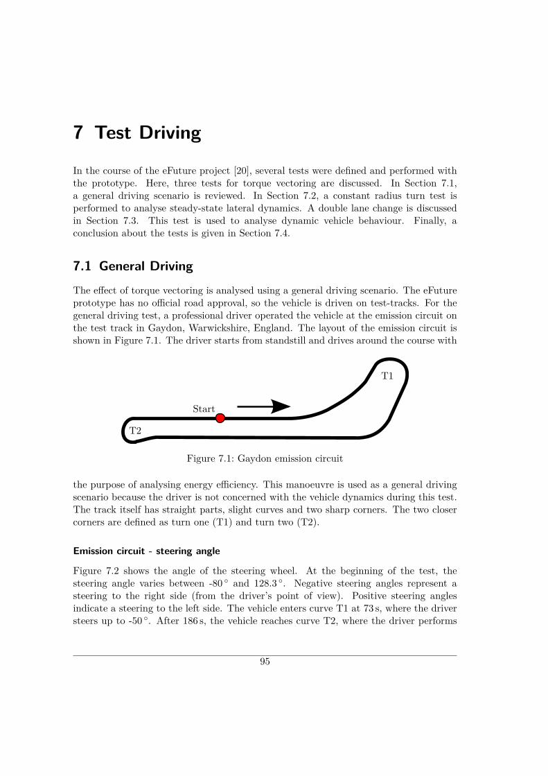
7 Test Driving
In the course of the eFuture project [20], several tests were defined and performed withthe prototype. Here, three tests for torque vectoring are discussed. In Section 7.1,a general driving scenario is reviewed. In Section 7.2, a constant radius turn test isperformed to analyse steady-state lateral dynamics. A double lane change is discussedin Section 7.3. This test is used to analyse dynamic vehicle behaviour. Finally, aconclusion about the tests is given in Section 7.4.
7.1 General Driving
The effect of torque vectoring is analysed using a general driving scenario. The eFutureprototype has no official road approval, so the vehicle is driven on test-tracks. For thegeneral driving test, a professional driver operated the vehicle at the emission circuit onthe test track in Gaydon, Warwickshire, England. The layout of the emission circuit isshown in Figure 7.1. The driver starts from standstill and drives around the course with
Start
T1
T2
Figure 7.1: Gaydon emission circuit
the purpose of analysing energy efficiency. This manoeuvre is used as a general drivingscenario because the driver is not concerned with the vehicle dynamics during this test.The track itself has straight parts, slight curves and two sharp corners. The two closercorners are defined as turn one (T1) and turn two (T2).
Emission circuit - steering angle
Figure 7.2 shows the angle of the steering wheel. At the beginning of the test, thesteering angle varies between -80 and 128.3 . Negative steering angles represent asteering to the right side (from the driver’s point of view). Positive steering anglesindicate a steering to the left side. The vehicle enters curve T1 at 73 s, where the driversteers up to -50 . After 186 s, the vehicle reaches curve T2, where the driver performs
95
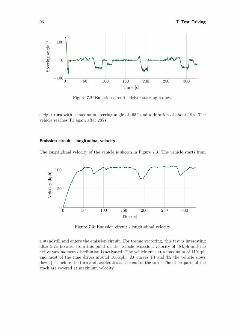
96 7 Test Driving
0 50 100 150 200 250 300−100
0
100
Time [s]
Stee
ring
angl
e[ ]
Figure 7.2: Emission circuit - driver steering request
a right turn with a maximum steering angle of -65 and a duration of about 19 s. Thevehicle reaches T1 again after 285 s.
Emission circuit - longitudinal velocity
The longitudinal velocity of the vehicle is shown in Figure 7.3. The vehicle starts from
0 50 100 150 200 250 3000
50
100
Time [s]
Velo
city
[kph
]
Figure 7.3: Emission circuit - longitudinal velocity
a standstill and enters the emission circuit. For torque vectoring, this test is interestingafter 5.2 s because from this point on the vehicle exceeds a velocity of 18 kph and theactive yaw moment distribution is activated. The vehicle runs at a maximum of 110 kphand most of the time drives around 106 kph. At curves T1 and T2 the vehicle slowsdown just before the turn and accelerates at the end of the turn. The other parts of thetrack are covered at maximum velocity.
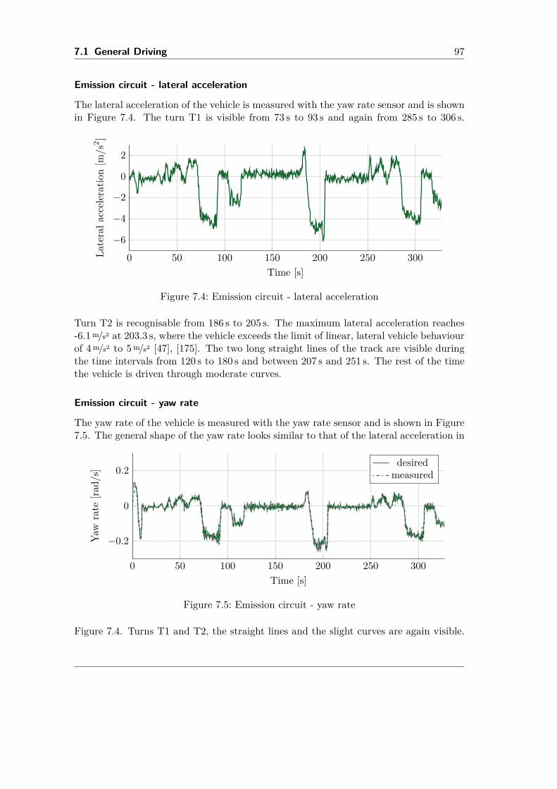
7.1 General Driving 97
Emission circuit - lateral acceleration
The lateral acceleration of the vehicle is measured with the yaw rate sensor and is shownin Figure 7.4. The turn T1 is visible from 73 s to 93 s and again from 285 s to 306 s.
0 50 100 150 200 250 300−6
−4
−2
0
2
Time [s]
Late
rala
ccel
erat
ion
[m/s
2 ]
Figure 7.4: Emission circuit - lateral acceleration
Turn T2 is recognisable from 186 s to 205 s. The maximum lateral acceleration reaches-6.1m/s2 at 203.3 s, where the vehicle exceeds the limit of linear, lateral vehicle behaviourof 4m/s2 to 5m/s2 [47], [175]. The two long straight lines of the track are visible duringthe time intervals from 120 s to 180 s and between 207 s and 251 s. The rest of the timethe vehicle is driven through moderate curves.
Emission circuit - yaw rate
The yaw rate of the vehicle is measured with the yaw rate sensor and is shown in Figure7.5. The general shape of the yaw rate looks similar to that of the lateral acceleration in
0 50 100 150 200 250 300
−0.2
0
0.2
Time [s]
Yaw
rate
[rad/
s]
desiredmeasured
Figure 7.5: Emission circuit - yaw rate
Figure 7.4. Turns T1 and T2, the straight lines and the slight curves are again visible.
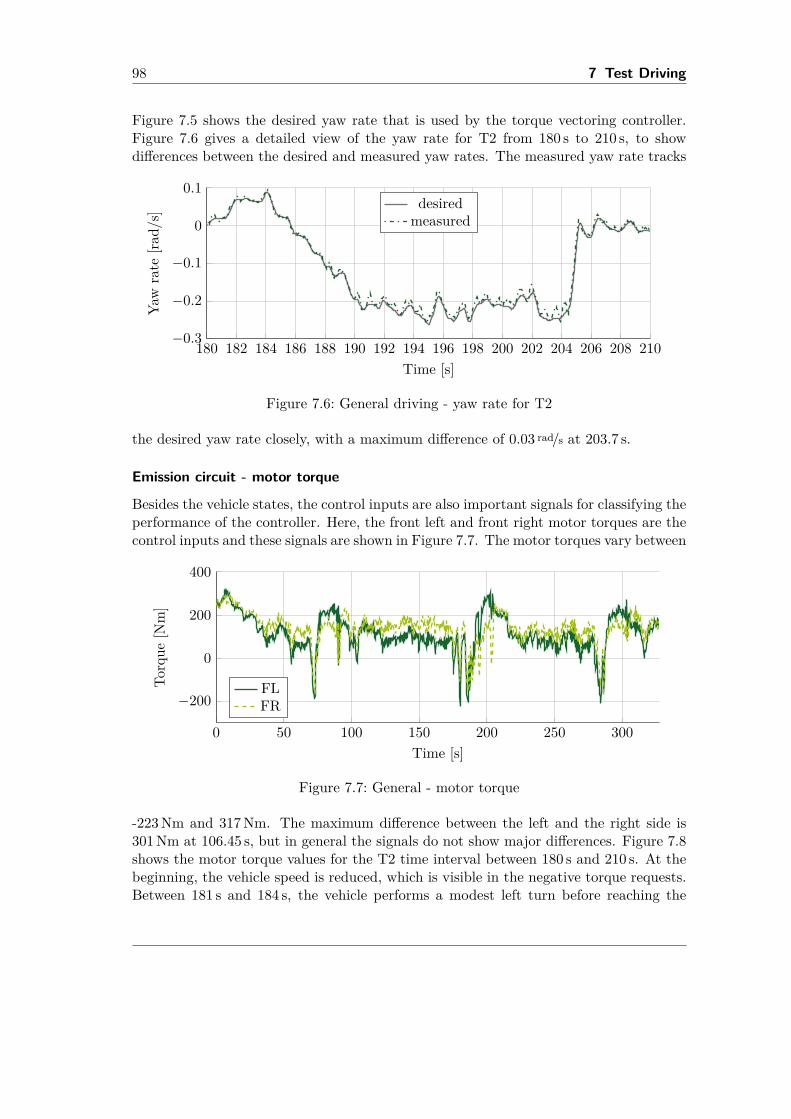
98 7 Test Driving
Figure 7.5 shows the desired yaw rate that is used by the torque vectoring controller.Figure 7.6 gives a detailed view of the yaw rate for T2 from 180 s to 210 s, to showdifferences between the desired and measured yaw rates. The measured yaw rate tracks
180 182 184 186 188 190 192 194 196 198 200 202 204 206 208 210−0.3
−0.2
−0.1
0
0.1
Time [s]
Yaw
rate
[rad/
s]
desiredmeasured
Figure 7.6: General driving - yaw rate for T2
the desired yaw rate closely, with a maximum difference of 0.03 rad/s at 203.7 s.
Emission circuit - motor torque
Besides the vehicle states, the control inputs are also important signals for classifying theperformance of the controller. Here, the front left and front right motor torques are thecontrol inputs and these signals are shown in Figure 7.7. The motor torques vary between
0 50 100 150 200 250 300
−200
0
200
400
Time [s]
Torq
ue[N
m]
FLFR
Figure 7.7: General - motor torque
-223Nm and 317Nm. The maximum difference between the left and the right side is301Nm at 106.45 s, but in general the signals do not show major differences. Figure 7.8shows the motor torque values for the T2 time interval between 180 s and 210 s. At thebeginning, the vehicle speed is reduced, which is visible in the negative torque requests.Between 181 s and 184 s, the vehicle performs a modest left turn before reaching the
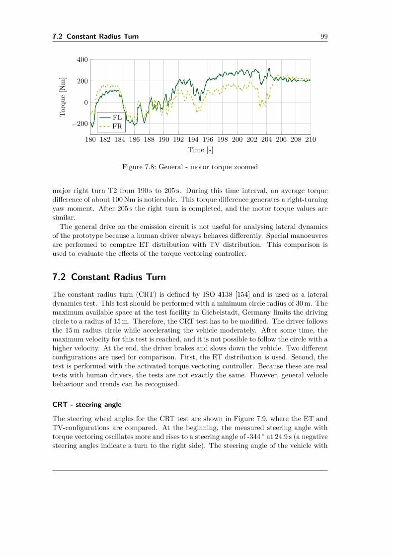
7.2 Constant Radius Turn 99
180 182 184 186 188 190 192 194 196 198 200 202 204 206 208 210
−200
0
200
400
Time [s]
Torq
ue[N
m]
FLFR
Figure 7.8: General - motor torque zoomed
major right turn T2 from 190 s to 205 s. During this time interval, an average torquedifference of about 100Nm is noticeable. This torque difference generates a right-turningyaw moment. After 205 s the right turn is completed, and the motor torque values aresimilar.The general drive on the emission circuit is not useful for analysing lateral dynamics
of the prototype because a human driver always behaves differently. Special manoeuvresare performed to compare ET distribution with TV distribution. This comparison isused to evaluate the effects of the torque vectoring controller.
7.2 Constant Radius Turn
The constant radius turn (CRT) is defined by ISO 4138 [154] and is used as a lateraldynamics test. This test should be performed with a minimum circle radius of 30m. Themaximum available space at the test facility in Giebelstadt, Germany limits the drivingcircle to a radius of 15m. Therefore, the CRT test has to be modified. The driver followsthe 15m radius circle while accelerating the vehicle moderately. After some time, themaximum velocity for this test is reached, and it is not possible to follow the circle with ahigher velocity. At the end, the driver brakes and slows down the vehicle. Two differentconfigurations are used for comparison. First, the ET distribution is used. Second, thetest is performed with the activated torque vectoring controller. Because these are realtests with human drivers, the tests are not exactly the same. However, general vehiclebehaviour and trends can be recognised.
CRT - steering angle
The steering wheel angles for the CRT test are shown in Figure 7.9, where the ET andTV-configurations are compared. At the beginning, the measured steering angle withtorque vectoring oscillates more and rises to a steering angle of -344 at 24.9 s (a negativesteering angles indicate a turn to the right side). The steering angle of the vehicle with
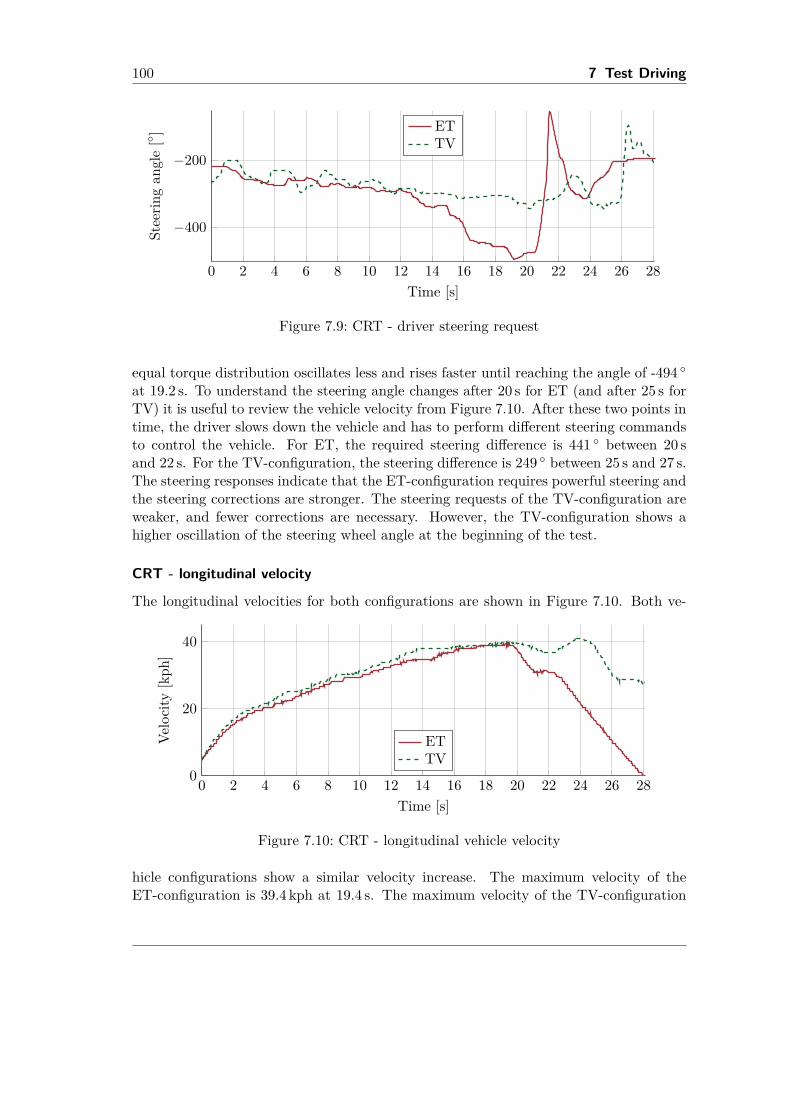
100 7 Test Driving
0 2 4 6 8 10 12 14 16 18 20 22 24 26 28
−400
−200
Time [s]
Stee
ring
angl
e[ ] ET
TV
Figure 7.9: CRT - driver steering request
equal torque distribution oscillates less and rises faster until reaching the angle of -494 at 19.2 s. To understand the steering angle changes after 20 s for ET (and after 25 s forTV) it is useful to review the vehicle velocity from Figure 7.10. After these two points intime, the driver slows down the vehicle and has to perform different steering commandsto control the vehicle. For ET, the required steering difference is 441 between 20 sand 22 s. For the TV-configuration, the steering difference is 249 between 25 s and 27 s.The steering responses indicate that the ET-configuration requires powerful steering andthe steering corrections are stronger. The steering requests of the TV-configuration areweaker, and fewer corrections are necessary. However, the TV-configuration shows ahigher oscillation of the steering wheel angle at the beginning of the test.
CRT - longitudinal velocity
The longitudinal velocities for both configurations are shown in Figure 7.10. Both ve-
0 2 4 6 8 10 12 14 16 18 20 22 24 26 280
20
40
Time [s]
Velo
city
[kph
]
ETTV
Figure 7.10: CRT - longitudinal vehicle velocity
hicle configurations show a similar velocity increase. The maximum velocity of theET-configuration is 39.4 kph at 19.4 s. The maximum velocity of the TV-configuration
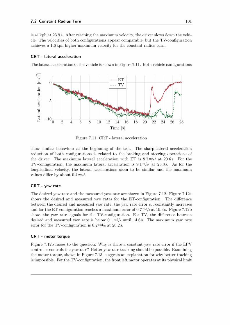
7.2 Constant Radius Turn 101
is 41 kph at 23.9 s. After reaching the maximum velocity, the driver slows down the vehi-cle. The velocities of both configurations appear comparable, but the TV-configurationachieves a 1.6 kph higher maximum velocity for the constant radius turn.
CRT - lateral acceleration
The lateral acceleration of the vehicle is shown in Figure 7.11. Both vehicle configurations
0 2 4 6 8 10 12 14 16 18 20 22 24 26 28−10
−5
0
Time [s]
Late
rala
ccel
erat
ion
[m/s
2 ]
ETTV
Figure 7.11: CRT - lateral acceleration
show similar behaviour at the beginning of the test. The sharp lateral accelerationreduction of both configurations is related to the braking and steering operations ofthe driver. The maximum lateral acceleration with ET is 8.7m/s2 at 20.6 s. For theTV-configuration, the maximum lateral acceleration is 9.1m/s2 at 25.3 s. As for thelongitudinal velocity, the lateral accelerations seem to be similar and the maximumvalues differ by about 0.4m/s2.
CRT - yaw rate
The desired yaw rate and the measured yaw rate are shown in Figure 7.12. Figure 7.12ashows the desired and measured yaw rates for the ET-configuration. The differencebetween the desired and measured yaw rate, the yaw rate error er, constantly increasesand for the ET-configuration reaches a maximum error of 0.7 rad/s at 19.3 s. Figure 7.12bshows the yaw rate signals for the TV-configuration. For TV, the difference betweendesired and measured yaw rate is below 0.1 rad/s until 14.6 s. The maximum yaw rateerror for the TV-configuration is 0.2 rad/s at 20.2 s.
CRT - motor torque
Figure 7.12b raises to the question: Why is there a constant yaw rate error if the LPVcontroller controls the yaw rate? Better yaw rate tracking should be possible. Examiningthe motor torque, shown in Figure 7.13, suggests an explanation for why better trackingis impossible. For the TV-configuration, the front left motor operates at its physical limit
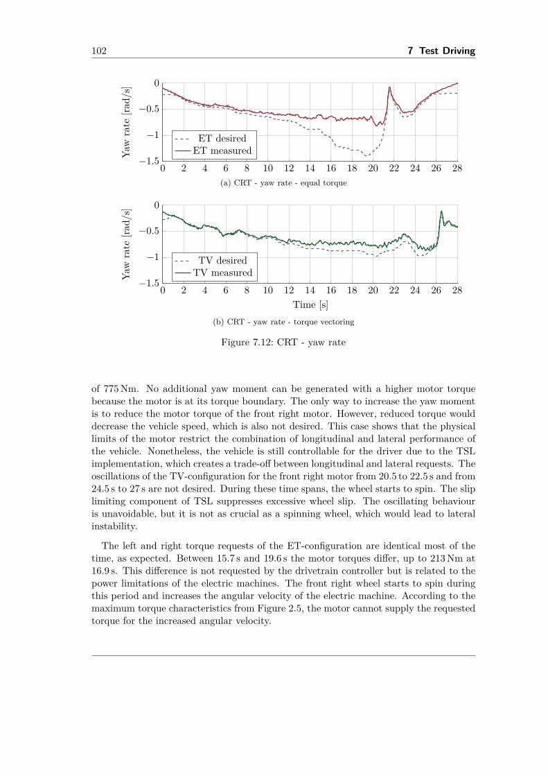
102 7 Test Driving
0 2 4 6 8 10 12 14 16 18 20 22 24 26 28−1.5
−1
−0.5
0
Yaw
rate
[rad/
s]ET desired
ET measured
(a) CRT - yaw rate - equal torque
0 2 4 6 8 10 12 14 16 18 20 22 24 26 28−1.5
−1
−0.5
0
Time [s]
Yaw
rate
[rad/
s]
TV desiredTV measured
(b) CRT - yaw rate - torque vectoring
Figure 7.12: CRT - yaw rate
of 775Nm. No additional yaw moment can be generated with a higher motor torquebecause the motor is at its torque boundary. The only way to increase the yaw momentis to reduce the motor torque of the front right motor. However, reduced torque woulddecrease the vehicle speed, which is also not desired. This case shows that the physicallimits of the motor restrict the combination of longitudinal and lateral performance ofthe vehicle. Nonetheless, the vehicle is still controllable for the driver due to the TSLimplementation, which creates a trade-off between longitudinal and lateral requests. Theoscillations of the TV-configuration for the front right motor from 20.5 to 22.5 s and from24.5 s to 27 s are not desired. During these time spans, the wheel starts to spin. The sliplimiting component of TSL suppresses excessive wheel slip. The oscillating behaviouris unavoidable, but it is not as crucial as a spinning wheel, which would lead to lateralinstability.
The left and right torque requests of the ET-configuration are identical most of thetime, as expected. Between 15.7 s and 19.6 s the motor torques differ, up to 213Nm at16.9 s. This difference is not requested by the drivetrain controller but is related to thepower limitations of the electric machines. The front right wheel starts to spin duringthis period and increases the angular velocity of the electric machine. According to themaximum torque characteristics from Figure 2.5, the motor cannot supply the requestedtorque for the increased angular velocity.
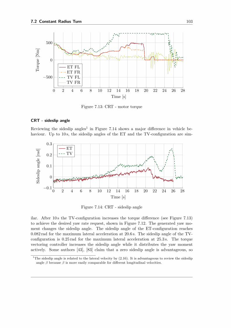
7.2 Constant Radius Turn 103
0 2 4 6 8 10 12 14 16 18 20 22 24 26 28
−500
0
500
Time [s]
Torq
ue[N
m]
ET FLET FRTV FLTV FR
Figure 7.13: CRT - motor torque
CRT - sideslip angle
Reviewing the sideslip angles1 in Figure 7.14 shows a major difference in vehicle be-haviour. Up to 10 s, the sideslip angles of the ET and the TV-configuration are sim-
0 2 4 6 8 10 12 14 16 18 20 22 24 26 28−0.1
0
0.1
0.2
0.3
Time [s]
Side
slip
angl
e[ra
d] ETTV
Figure 7.14: CRT - sideslip angle
ilar. After 10 s the TV-configuration increases the torque difference (see Figure 7.13)to achieve the desired yaw rate request, shown in Figure 7.12. The generated yaw mo-ment changes the sideslip angle. The sideslip angle of the ET-configuration reaches0.082 rad for the maximum lateral acceleration at 20.6 s. The sideslip angle of the TV-configuration is 0.25 rad for the maximum lateral acceleration at 25.3 s. The torquevectoring controller increases the sideslip angle while it distributes the yaw momentactively. Some authors [43], [83] claim that a zero sideslip angle is advantageous, so
1The sideslip angle is related to the lateral velocity by (2.16). It is advantageous to review the sideslipangle β because β is more easily comparable for different longitudinal velocities.
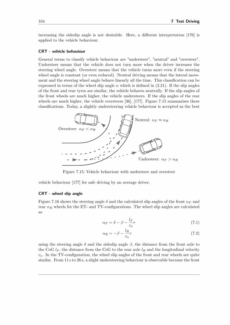
104 7 Test Driving
increasing the sideslip angle is not desirable. Here, a different interpretation [176] isapplied to the vehicle behaviour.
CRT - vehicle behaviour
General terms to classify vehicle behaviour are "understeer", "neutral" and "oversteer".Understeer means that the vehicle does not turn more when the driver increases thesteering wheel angle. Oversteer means that the vehicle turns more even if the steeringwheel angle is constant (or even reduced). Neutral driving means that the lateral move-ment and the steering wheel angle behave linearly all the time. This classification can beexpressed in terms of the wheel slip angle α which is defined in (2.21). If the slip anglesof the front and rear tyres are similar, the vehicle behaves neutrally. If the slip angles ofthe front wheels are much higher, the vehicle understeers. If the slip angles of the rearwheels are much higher, the vehicle oversteers [36], [177]. Figure 7.15 summarises theseclassifications. Today, a slightly understeering vehicle behaviour is accepted as the best
Neutral: αF ≈ αR
Understeer: αF > αR
Oversteer: αF < αR
Figure 7.15: Vehicle behaviour with understeer and oversteer
vehicle behaviour [177] for safe driving by an average driver.
CRT - wheel slip angle
Figure 7.16 shows the steering angle δ and the calculated slip angles of the front αF andrear αR wheels for the ET- and TV-configurations. The wheel slip angles are calculatedas
αF = δ − β − lFvxr (7.1)
αR = −β − lRvxr (7.2)
using the steering angle δ and the sideslip angle β, the distance from the front axle tothe CoG lF , the distance from the CoG to the rear axle lR and the longitudinal velocityvx. In the TV-configuration, the wheel slip angles of the front and rear wheels are quitesimilar. From 11 s to 26 s, a slight understeering behaviour is observable because the front
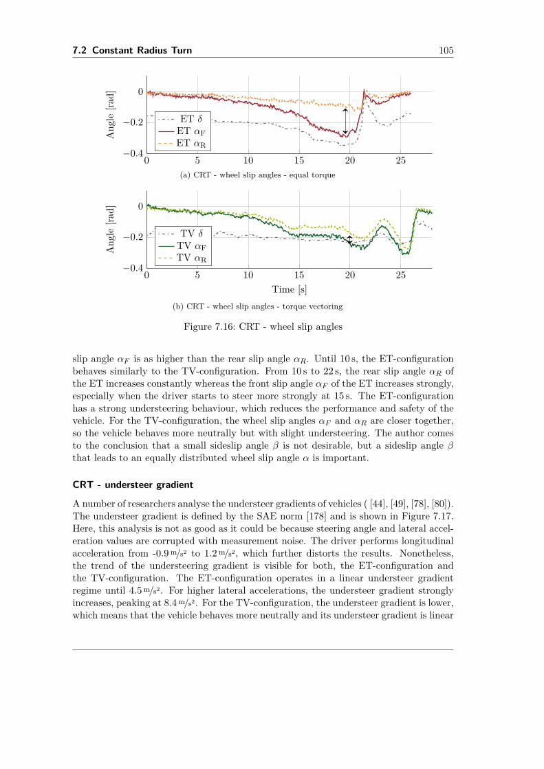
7.2 Constant Radius Turn 105
0 5 10 15 20 25−0.4
−0.2
0A
ngle
[rad]
ET δET αFET αR
(a) CRT - wheel slip angles - equal torque
0 5 10 15 20 25−0.4
−0.2
0
Time [s]
Ang
le[ra
d]
TV δTV αFTV αR
(b) CRT - wheel slip angles - torque vectoring
Figure 7.16: CRT - wheel slip angles
slip angle αF is as higher than the rear slip angle αR. Until 10 s, the ET-configurationbehaves similarly to the TV-configuration. From 10 s to 22 s, the rear slip angle αR ofthe ET increases constantly whereas the front slip angle αF of the ET increases strongly,especially when the driver starts to steer more strongly at 15 s. The ET-configurationhas a strong understeering behaviour, which reduces the performance and safety of thevehicle. For the TV-configuration, the wheel slip angles αF and αR are closer together,so the vehicle behaves more neutrally but with slight understeering. The author comesto the conclusion that a small sideslip angle β is not desirable, but a sideslip angle βthat leads to an equally distributed wheel slip angle α is important.
CRT - understeer gradient
A number of researchers analyse the understeer gradients of vehicles ( [44], [49], [78], [80]).The understeer gradient is defined by the SAE norm [178] and is shown in Figure 7.17.Here, this analysis is not as good as it could be because steering angle and lateral accel-eration values are corrupted with measurement noise. The driver performs longitudinalacceleration from -0.9m/s2 to 1.2m/s2, which further distorts the results. Nonetheless,the trend of the understeering gradient is visible for both, the ET-configuration andthe TV-configuration. The ET-configuration operates in a linear understeer gradientregime until 4.5m/s2. For higher lateral accelerations, the understeer gradient stronglyincreases, peaking at 8.4m/s2. For the TV-configuration, the understeer gradient is lower,which means that the vehicle behaves more neutrally and its understeer gradient is linear
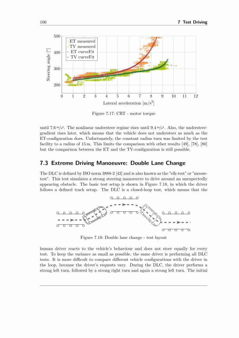
106 7 Test Driving
0 1 2 3 4 5 6 7 8 9 10 11 12
200
300
400
500
Lateral acceleration [m/s2]
Stee
ring
angl
e[ ]
ET measuredTV measuredET curveFitTV curveFit
Figure 7.17: CRT - motor torque
until 7.6m/s2. The nonlinear understeer regime rises until 9.4m/s2. Also, the understeer-gradient rises later, which means that the vehicle does not understeer as much as theET-configuration does. Unfortunately, the constant radius turn was limited by the testfacility to a radius of 15m. This limits the comparison with other results [49], [78], [80]but the comparison between the ET and the TV-configuration is still possible.
7.3 Extreme Driving Manoeuvre: Double Lane ChangeThe DLC is defined by ISO norm 3888-2 [42] and is also known as the "elk-test" or "moose-test". This test simulates a strong steering manoeuvre to drive around an unexpectedlyappearing obstacle. The basic test setup is shown in Figure 7.18, in which the driverfollows a defined track setup. The DLC is a closed-loop test, which means that the
Figure 7.18: Double lane change - test layout
human driver reacts to the vehicle’s behaviour and does not steer equally for everytest. To keep the variance as small as possible, the same driver is performing all DLCtests. It is more difficult to compare different vehicle configurations with the driver inthe loop, because the driver’s requests vary. During the DLC, the driver performs astrong left turn, followed by a strong right turn and again a strong left turn. The initial
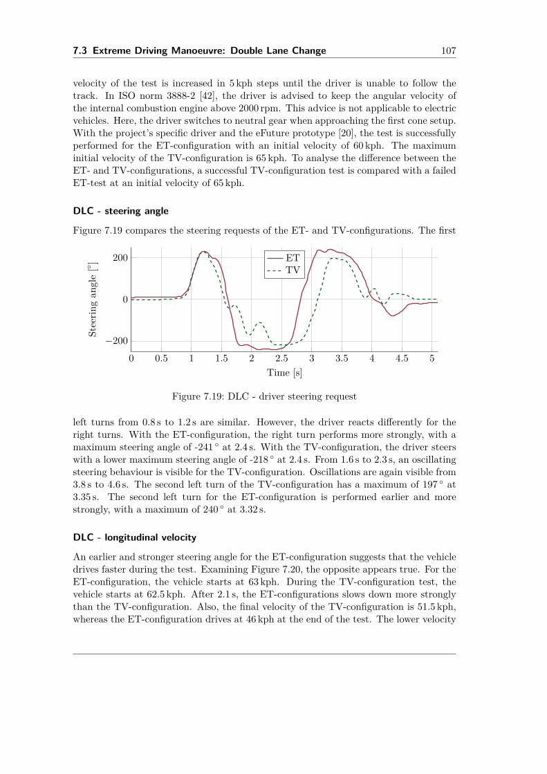
7.3 Extreme Driving Manoeuvre: Double Lane Change 107
velocity of the test is increased in 5 kph steps until the driver is unable to follow thetrack. In ISO norm 3888-2 [42], the driver is advised to keep the angular velocity ofthe internal combustion engine above 2000 rpm. This advice is not applicable to electricvehicles. Here, the driver switches to neutral gear when approaching the first cone setup.With the project’s specific driver and the eFuture prototype [20], the test is successfullyperformed for the ET-configuration with an initial velocity of 60 kph. The maximuminitial velocity of the TV-configuration is 65 kph. To analyse the difference between theET- and TV-configurations, a successful TV-configuration test is compared with a failedET-test at an initial velocity of 65 kph.
DLC - steering angle
Figure 7.19 compares the steering requests of the ET- and TV-configurations. The first
0 0.5 1 1.5 2 2.5 3 3.5 4 4.5 5−200
0
200
Time [s]
Stee
ring
angl
e[ ] ET
TV
Figure 7.19: DLC - driver steering request
left turns from 0.8 s to 1.2 s are similar. However, the driver reacts differently for theright turns. With the ET-configuration, the right turn performs more strongly, with amaximum steering angle of -241 at 2.4 s. With the TV-configuration, the driver steerswith a lower maximum steering angle of -218 at 2.4 s. From 1.6 s to 2.3 s, an oscillatingsteering behaviour is visible for the TV-configuration. Oscillations are again visible from3.8 s to 4.6 s. The second left turn of the TV-configuration has a maximum of 197 at3.35 s. The second left turn for the ET-configuration is performed earlier and morestrongly, with a maximum of 240 at 3.32 s.
DLC - longitudinal velocity
An earlier and stronger steering angle for the ET-configuration suggests that the vehicledrives faster during the test. Examining Figure 7.20, the opposite appears true. For theET-configuration, the vehicle starts at 63 kph. During the TV-configuration test, thevehicle starts at 62.5 kph. After 2.1 s, the ET-configurations slows down more stronglythan the TV-configuration. Also, the final velocity of the TV-configuration is 51.5 kph,whereas the ET-configuration drives at 46 kph at the end of the test. The lower velocity
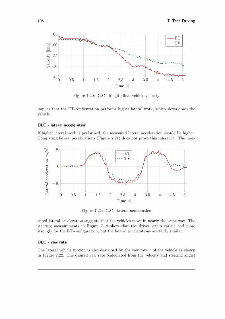
108 7 Test Driving
0 0.5 1 1.5 2 2.5 3 3.5 4 4.5 545
50
55
60
65
Time [s]
Velo
city
[kph
]
ETTV
Figure 7.20: DLC - longitudinal vehicle velocity
implies that the ET-configuration performs higher lateral work, which slows down thevehicle.
DLC - lateral acceleration
If higher lateral work is performed, the measured lateral acceleration should be higher.Comparing lateral accelerations (Figure 7.21) does not prove this inference. The mea-
0 0.5 1 1.5 2 2.5 3 3.5 4 4.5 5
−10
0
10
Time [s]
Late
rala
ccel
erat
ion
[m/s
2 ]
ETTV
Figure 7.21: DLC - lateral acceleration
sured lateral acceleration suggests that the vehicles move in nearly the same way. Thesteering measurements in Figure 7.19 show that the driver steers earlier and morestrongly for the ET-configuration, but the lateral accelerations are fairly similar.
DLC - yaw rate
The lateral vehicle motion is also described by the yaw rate r of the vehicle as shownin Figure 7.22. The desired yaw rate (calculated from the velocity and steering angle)
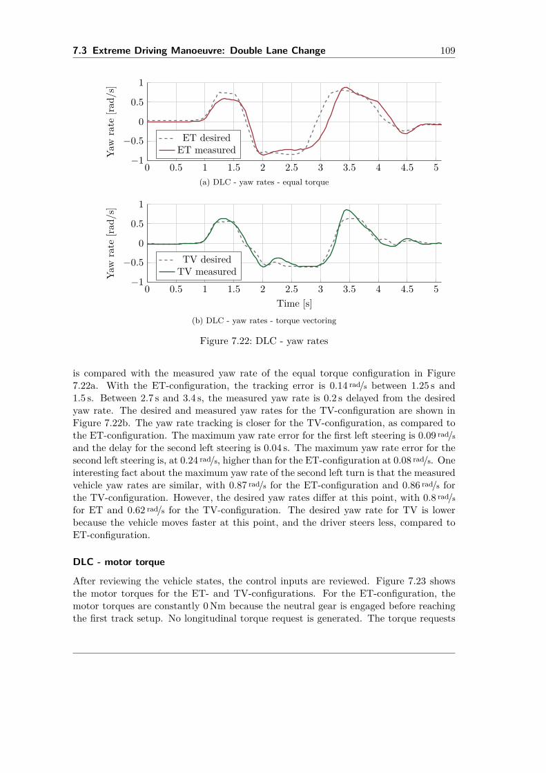
7.3 Extreme Driving Manoeuvre: Double Lane Change 109
0 0.5 1 1.5 2 2.5 3 3.5 4 4.5 5−1
−0.5
0
0.5
1
Yaw
rate
[rad/
s]
ET desiredET measured
(a) DLC - yaw rates - equal torque
0 0.5 1 1.5 2 2.5 3 3.5 4 4.5 5−1
−0.5
0
0.5
1
Time [s]
Yaw
rate
[rad/
s]
TV desiredTV measured
(b) DLC - yaw rates - torque vectoring
Figure 7.22: DLC - yaw rates
is compared with the measured yaw rate of the equal torque configuration in Figure7.22a. With the ET-configuration, the tracking error is 0.14 rad/s between 1.25 s and1.5 s. Between 2.7 s and 3.4 s, the measured yaw rate is 0.2 s delayed from the desiredyaw rate. The desired and measured yaw rates for the TV-configuration are shown inFigure 7.22b. The yaw rate tracking is closer for the TV-configuration, as compared tothe ET-configuration. The maximum yaw rate error for the first left steering is 0.09 rad/sand the delay for the second left steering is 0.04 s. The maximum yaw rate error for thesecond left steering is, at 0.24 rad/s, higher than for the ET-configuration at 0.08 rad/s. Oneinteresting fact about the maximum yaw rate of the second left turn is that the measuredvehicle yaw rates are similar, with 0.87 rad/s for the ET-configuration and 0.86 rad/s forthe TV-configuration. However, the desired yaw rates differ at this point, with 0.8 rad/sfor ET and 0.62 rad/s for the TV-configuration. The desired yaw rate for TV is lowerbecause the vehicle moves faster at this point, and the driver steers less, compared toET-configuration.
DLC - motor torque
After reviewing the vehicle states, the control inputs are reviewed. Figure 7.23 showsthe motor torques for the ET- and TV-configurations. For the ET-configuration, themotor torques are constantly 0Nm because the neutral gear is engaged before reachingthe first track setup. No longitudinal torque request is generated. The torque requests
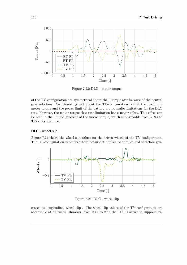
110 7 Test Driving
0 0.5 1 1.5 2 2.5 3 3.5 4 4.5 5−1,000
−500
0
500
1,000
Time [s]
Torq
ue[N
m]
ET FLET FRTV FLTV FR
Figure 7.23: DLC - motor torque
of the TV-configuration are symmetrical about the 0 torque axis because of the neutralgear selection. An interesting fact about the TV-configuration is that the maximummotor torque and the power limit of the battery are no major limitations for the DLCtest. However, the motor torque slew-rate limitation has a major effect. This effect canbe seen in the limited gradient of the motor torque, which is observable from 3.09 s to3.27 s, for example.
DLC - wheel slip
Figure 7.24 shows the wheel slip values for the driven wheels of the TV-configuration.The ET-configuration is omitted here because it applies no torques and therefore gen-
0 0.5 1 1.5 2 2.5 3 3.5 4 4.5 5
−0.2
0
Time [s]
Whe
elsli
p
TV FLTV FR
Figure 7.24: DLC - wheel slip
erates no longitudinal wheel slips. The wheel slip values of the TV-configuration areacceptable at all times. However, from 2.4 s to 2.6 s the TSL is active to suppress ex-
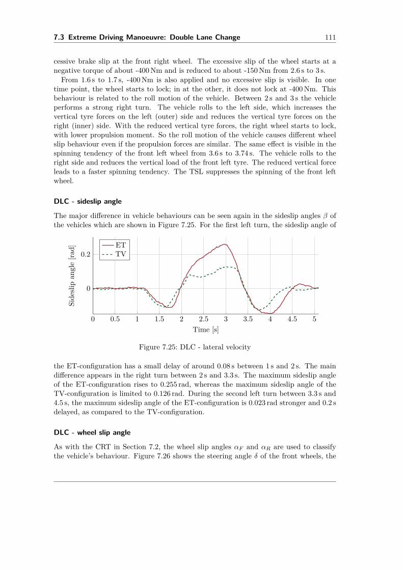
7.3 Extreme Driving Manoeuvre: Double Lane Change 111
cessive brake slip at the front right wheel. The excessive slip of the wheel starts at anegative torque of about -400Nm and is reduced to about -150Nm from 2.6 s to 3 s.From 1.6 s to 1.7 s, -400Nm is also applied and no excessive slip is visible. In one
time point, the wheel starts to lock; in at the other, it does not lock at -400Nm. Thisbehaviour is related to the roll motion of the vehicle. Between 2 s and 3 s the vehicleperforms a strong right turn. The vehicle rolls to the left side, which increases thevertical tyre forces on the left (outer) side and reduces the vertical tyre forces on theright (inner) side. With the reduced vertical tyre forces, the right wheel starts to lock,with lower propulsion moment. So the roll motion of the vehicle causes different wheelslip behaviour even if the propulsion forces are similar. The same effect is visible in thespinning tendency of the front left wheel from 3.6 s to 3.74 s. The vehicle rolls to theright side and reduces the vertical load of the front left tyre. The reduced vertical forceleads to a faster spinning tendency. The TSL suppresses the spinning of the front leftwheel.
DLC - sideslip angle
The major difference in vehicle behaviours can be seen again in the sideslip angles β ofthe vehicles which are shown in Figure 7.25. For the first left turn, the sideslip angle of
0 0.5 1 1.5 2 2.5 3 3.5 4 4.5 5
0
0.2
Time [s]
Side
slip
angl
e[ra
d] ETTV
Figure 7.25: DLC - lateral velocity
the ET-configuration has a small delay of around 0.08 s between 1 s and 2 s. The maindifference appears in the right turn between 2 s and 3.3 s. The maximum sideslip angleof the ET-configuration rises to 0.255 rad, whereas the maximum sideslip angle of theTV-configuration is limited to 0.126 rad. During the second left turn between 3.3 s and4.5 s, the maximum sideslip angle of the ET-configuration is 0.023 rad stronger and 0.2 sdelayed, as compared to the TV-configuration.
DLC - wheel slip angle
As with the CRT in Section 7.2, the wheel slip angles αF and αR are used to classifythe vehicle’s behaviour. Figure 7.26 shows the steering angle δ of the front wheels, the
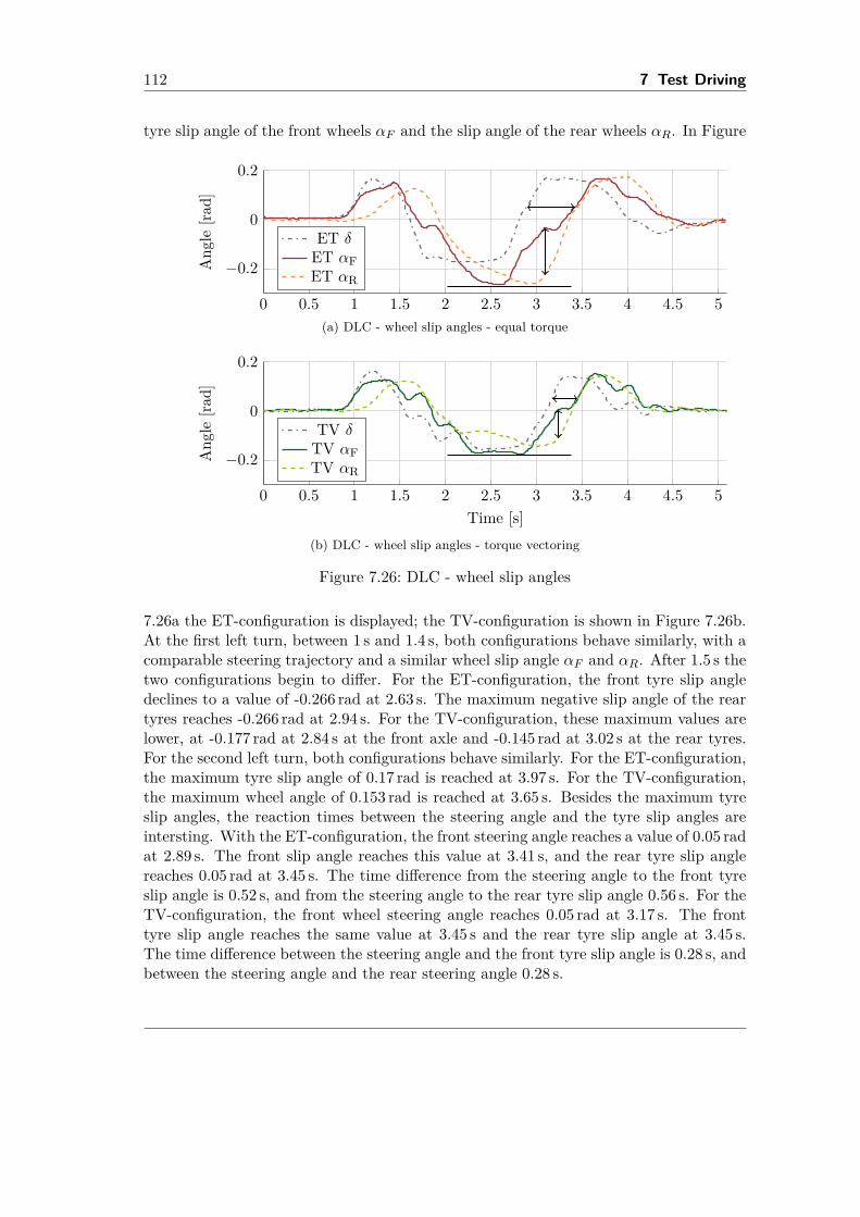
112 7 Test Driving
tyre slip angle of the front wheels αF and the slip angle of the rear wheels αR. In Figure
0 0.5 1 1.5 2 2.5 3 3.5 4 4.5 5
−0.2
0
0.2
Ang
le[ra
d]
ET δET αFET αR
(a) DLC - wheel slip angles - equal torque
0 0.5 1 1.5 2 2.5 3 3.5 4 4.5 5
−0.2
0
0.2
Time [s]
Ang
le[ra
d]
TV δTV αFTV αR
(b) DLC - wheel slip angles - torque vectoring
Figure 7.26: DLC - wheel slip angles
7.26a the ET-configuration is displayed; the TV-configuration is shown in Figure 7.26b.At the first left turn, between 1 s and 1.4 s, both configurations behave similarly, with acomparable steering trajectory and a similar wheel slip angle αF and αR. After 1.5 s thetwo configurations begin to differ. For the ET-configuration, the front tyre slip angledeclines to a value of -0.266 rad at 2.63 s. The maximum negative slip angle of the reartyres reaches -0.266 rad at 2.94 s. For the TV-configuration, these maximum values arelower, at -0.177 rad at 2.84 s at the front axle and -0.145 rad at 3.02 s at the rear tyres.For the second left turn, both configurations behave similarly. For the ET-configuration,the maximum tyre slip angle of 0.17 rad is reached at 3.97 s. For the TV-configuration,the maximum wheel angle of 0.153 rad is reached at 3.65 s. Besides the maximum tyreslip angles, the reaction times between the steering angle and the tyre slip angles areintersting. With the ET-configuration, the front steering angle reaches a value of 0.05 radat 2.89 s. The front slip angle reaches this value at 3.41 s, and the rear tyre slip anglereaches 0.05 rad at 3.45 s. The time difference from the steering angle to the front tyreslip angle is 0.52 s, and from the steering angle to the rear tyre slip angle 0.56 s. For theTV-configuration, the front wheel steering angle reaches 0.05 rad at 3.17 s. The fronttyre slip angle reaches the same value at 3.45 s and the rear tyre slip angle at 3.45 s.The time difference between the steering angle and the front tyre slip angle is 0.28 s, andbetween the steering angle and the rear steering angle 0.28 s.
7.4 Test Driving: Conclusion 113
The arrows and the black line at the bottom are introduced to visualise the differencesbetween Figure 7.26a and Figure 7.26b. The lengths of the vertical arrows indicate thedifferent vehicle behaviours. The bottom line indicates the reduced maximum wheel slipangle α of the TV-configuration. The horizontal arrows indicate the reduced time delayof the TV-configuration, compared to the ET-configuration.
DLC - vehicle behaviour
Using the definitions from Figure 7.15, the vehicle behaviour can be described by theterms understeer, oversteer and neutral operation. During the DLC, the ET-configurationhas an understeering behaviour between 1 s and 1.5 s. Between 1.5 s and 1.9 s, the vehi-cle has an oversteering behaviour. Between 1.9 s and 2.7 s, the ET-configuration slightlyundersteers. Between 2.7 s and 3.4 s, the vehicle has a strong oversteering behaviour,which is followed by a neutral phase between 3.4 s and 3.8 s. Between 3.8 s and 4.3 s, thevehicle slightly oversteers. Afterwards, the vehicle behaves neutrally.The TV-configuration generally behaves like the ET-configuration with phases of un-
dersteering (1 - 1.4 s), oversteering (1.4 - 1.9 s), understeering (1.9 - 2.9 s), oversteering(2.9 - 3.4 s), neutral (3.4 - 3.7 s), and oversteering (3.7 - 4.2 s). The understeering phasesare similar. However, the oversteering phases are weaker with the TV-configuration.The most extreme example of oversteering is the second oversteering phase, where themaximum angle between the front and rear tyre slip angles is 0.191 rad at 3.06 s for theET-configuration and 0.115 rad at 3.22 s for the TV-configuration. As a result the TV-configuration has only an 60% oversteering tendency, compared to the ET-configuration.
7.4 Test Driving: ConclusionTo analyse the lateral vehicle behaviour, several tests are performed. A general drivingscenario, the constant radius turn and the double lane change are analysed. For thegeneral driving scenario, only the function of torque vectoring is tested. A comparisonwith the equal torque distribution was not possible because no similar test drives wereavailable. The constant radius turn is a static lateral test, and allows a torque vectoringvehicle to be compared with an equal torque distribution vehicle.With torque vectoring,the driver has to steer less to follow the desired circle and the velocity of the vehicleis about 1.5 kph higher. More important, if torque vectoring is activated, the innerwheel does not spin. It is possible to steer the vehicle because the TSL suppressesexcessive wheel slip and tyre abrasion is reduced. Additionally, this test shows thereduced understeering behaviour of the vehicle with torque vectoring. The double lanechange is a dynamic lateral test, which forces vehicles to oversteer. With activated torquevectoring, the driver successfully performs the DLC with an initial velocity of 65 kph.With equal torque, the driver successfully performs this test only at 60 kph. Hence, theperformance and safety of the vehicle with TV are superior. Objective criteria, reflectedin the yaw rate tracking and wheel slip angle analyses, show a faster vehicle response tosteering requests. With torque vectoring, the vehicle behaves more neutrally. The delaytime between steering wheel movement and vehicle response is reduced.
114 7 Test Driving
Several tests were performed with the eFuture prototype [20]. Drivers liked the quickerresponse of the vehicle and the smoother steering wheel feeling during curves. Unfortu-nately, drivers reported an undesirable oscillation of the steering wheel when they drovestraight. Apart from that problem, the vehicle reacted quicker and accurately to therequests given. Straight line braking and accelerating tests were performed as longitu-dinal tests. No striking results were obtained there, only confirmation that the vehiclebehaves as expected by the driver.Remark 7.1 The steering wheel oscillations of the eFuture prototype [20] are related todistributed front wheel forces and the "direct" steering column. The eFuture prototype isequipped with mechanical front wheel steering with no power-assisted steering. Vehicleswith servo-power-assisted steering would create smaller feedback forces at the steeringwheel. If the vehicle is equipped with active steering or steer by wire devices, this effectcan be suppressed completely.
8 General Conclusions and Future WorkThis chapter provides a conclusion to the thesis and an outlook for interesting topicsthat arose during this study and will be addressed in the future.
8.1 General ConclusionsThe dynamics of an automotive vehicle are explained in Section 2. The basic equations ofmotion are introduced, and a three-dimensional vehicle model is generated. This modelhas 14 degrees of freedom and the vehicle model can move in all three axes in space,rotate around all three axes, and its suspension movement is governed. This modelis used for the development of different vehicle functions in the eFuture project [20].Additionally, the model is integrated into the driving simulator from WIVW [150]. It ispossible to operate this simulator on a computer with standard computer components,or inside a real hydraulic test environment that simulates the forces acting on a driverin a real vehicle. The main challenges in these simulations are calculating tyre forceexactly. Different tyre models from the literature are reviewed, and the Dugoff tyremodel [38] and the Pacejka tyre model [36] are calibrated following real test drives.However, the three-dimensional model is too complex to implement a torque vectoringcontroller based on this model. A simplified single-track model is extracted from thethree-dimensional model, and this simple model is used for the controller design. Afterthe controller synthesis, the controller is validated with the 14 degrees of freedom modelfor proper operation.Before designing the torque vectoring controller, a review of actual torque vectoring
controller designs is given in Section 3. Various control strategies are extracted, and themajor inputs and outputs are described. Commonly used controller synthesis proceduresare summarised. Additionally, the non-linearity of the single-track vehicle model isanalysed, and requirements for torque vectoring are explained. Finally, an LPV basedcontrol concept is chosen because it combines the well known linear control strategiesfor optimal and robust control with the non-linear nature of the single-track model.The LFT-LPV and the polytopic LPV controller designs are described in Chapter 4.
Both designs use parameter-dependent plants, and the controllers calculated guaranteestability and performance. The controllers achieve similar results, and the main differ-ences are related to different tunings of the controller. However, the LFT-LPV controllercannot be implemented here because the design uses a parameter-dependent Lyapunovfunction, which requires a matrix-inversion inside the microcontroller. The polytopicLPV controller obtains similar simulation results and seems preferable in terms of thenumerical robustness of the solution and computation effort, and is chosen as the vehicledynamics controller.
115
116 8 General Conclusions and Future Work
An anti-windup scheme is developed for the LPV controller because the controller mustbe tuned aggressively to achieve good performance. However, an aggressive controllermight drive the actuators to physical limitations. These limitations are not includedin the controller design and degrade the performance of the vehicle and may even leadto instability. Additionally, the actuator limitations are not fixed and depend on manyparameters, such as the velocity of the vehicle, the temperature, the power consumption,the status of the battery and efficiency requests from the driver. The proposed anti-windup scheme improves the performance of the closed-loop system as far as possible.Besides addressing the limitations of the electric machines, the anti-windup scheme isextended to the TSL, where wheel slip limitations for safe vehicle operation are includedas actuator constraints. With this extension, the propulsion wheels do not spin orlock. The combination of LPV controller and TSL works nicely and improves vehicleperformance. However, natural physical limits cannot be exceeded, and the vehicle’sperformance can only be improved within these boundaries.Chapter 6 gives an overview of the necessary steps for implementation of the controller
into an automotive microcontroller. These steps could have been directly included inChapters 4 and 5. However, it seemed better to show the general controller developmentin the familiar continuous-time representation, and to use Chapter 6 for the requireddiscretisation and fixed-point conversion. Other drivetrain functions interacting withtorque vectoring are briefly described, and the range of torque vectoring activation isdiscussed. Finally, the implementation of a polytopic LPV controller for vehicle dynamicsin a standard automotive microcontroller, satisfying AUTOSAR standards, is described.Following validation of the virtual controller, the software is implemented in the mi-
crocontroller and tested in the vehicle. Various tests have been performed, and threerelevant tests for torque vectoring are described. A general driving scenario is analysedin order to clarify torque vectoring in an average, daily drive and to illustrate propercontrol of the vehicle. Afterwards, a constant radius turn is reviewed to examine vehi-cle movement in a constant, lateral behaviour. The difference between an equal torquedistribution and the torque vectoring controller is analysed. The understeering of thevehicle is improved with torque vectoring, and the driver can follow the requested tra-jectory more easily. The maximum possible velocity is higher with the torque vectoringcontroller. Excessive wheel slip is suppressed, which improves the handling of the ve-hicle. A double lane change is also reviewed. This test analyses the dynamic, lateralperformance of the vehicle. The test driver was able to perform the test with an 8%higher initial velocity. However, the major result from this test is the faster reactionof the vehicle with torque vectoring to given steering inputs. The faster response im-proves the agility and "fun to drive" aspect of the vehicle. Additionally, the oversteeringtendency of the vehicle is reduced, which improves the safety of the vehicle in criticalmanoeuvres. These three tests showed that calibrating the desired vehicle states, tuningthe LPV controller, and adjusting the torque slip limiter are complex and challengingtasks.Nonetheless, vehicle performance is positively improved with the torque vectoring
controller. The wheels do not spin or lock because of the slip limitation characteristicsof the TSL component. The TSL prevents motor saturation and avoids overshoots and
8.2 Future Work 117
oscillations that are related to motor saturations. The LPV controller improves theperformance and safety of the vehicle by controlling the yaw rate and the longitudinalvelocity. The understeering of the vehicle is reduced, which is demonstrated by theconstant radius turn. The double lane change naturally forces the vehicle to oversteerbut the torque vectoring controller reduced the oversteering behaviour and improved thehandling of the vehicle.The main achievements of this thesis are the development and implementation of an
LPV controller for an electric drivetrain with two independent front motors. The con-troller can be activated during normal driving and improves the vehicle’s behaviour insafety critical driving conditions. When the torque vectoring controller was activatedthe vehicle never skidded during several tests, whereas the vehicle skidded at least fourtimes when using the equal torque distribution configuration, according to the author’sknowledge. Additionally, the combination of an anti-windup scheme with the desiredwheel slip limitation is a major result of this work. The concept of implementing limi-tations of model properties (wheel slip) as actuator limits rather than as model statescould be interesting for other applications that are under-actuated.
8.2 Future Work
The main disadvantage of the proposed torque vectoring controller is the feedback ofthe front wheel torque difference to the steering wheel. For the constant radius turn,this feeling is helpful to the driver because it reduces the arm force needed to steerthe vehicle. For the DLC or straight line driving, the feedback leads to an oscillatingsteering behaviour. This problem is noticeable in the prototype because no steeringsupport is integrated, and the steering wheel is directly linked to the front wheels. Withservo-assisted steering, this feedback is reduced. Active front steering or steer by wiretechnology would suppress this feedback successfully. This effect also vanishes completelyif torque vectoring is applied to the rear wheels.The understeering behaviour cannot be corrected for a front-wheel-drive vehicle as well
as it can for a four-wheel-drive vehicle. It is beneficial to apply longitudinal wheel forcesat the rear wheel if the vehicle understeers. During understeering, lateral forces of thefront wheels are saturated, and additional longitudinal forces do not solve this problemand may even worsen it. Here the understeering of the vehicle is improved because thetorque applied to the inside front tyre is reduced, and the outside front wheel force isincreased. The outside wheel is not as crucial because the vertical load of the outsidewheel is higher and the outside wheel can generate higher lateral forces. However, theundersteering could be corrected more efficiently by applying longitudinal forces to therear wheels. With oversteering, it is the other way around. Applying longitudinal forcesonly to the outside wheel is beneficial but it is better to apply longitudinal forces to thefront wheels. With four independent electric machines, oversteering and understeeringcan be corrected efficiently. Furthermore, the force difference at the front wheels can beused to improve the steering wheel feeling for the driver.Besides the general drivetrain layout of the prototype, the tuning of the vehicle dy-
118 8 General Conclusions and Future Work
namics simulation model should be improved in the future. At present, model tuningis performed heuristically, which requires time and knowledge. Especially the tuningof the tyre forces is complicated. An appropriate identification algorithm that uses theexisting sensor signals and vehicle parameters should solve this problem.For controller synthesis, an affine LFT-LPV controller should be tested in the future.
The polytopic controller achieved positive results and seemed to be the safest solutionfor implementing the controller because no major implementation drawbacks were vis-ible. However, the demands on the structure of the model imply undesirable designlimitations. For example, it would be beneficial to consider the air-drag of the vehiclein the controller design, without increasing the number of scheduling parameters. Inthis way, the LPV controller could deal directly with the disturbance. Including airdrag and using a less demanding controller implementation [140] should further improvethe LPV controller in terms of performance and implementation complexity. Designingmore sophisticated parameter-dependent shaping filters should also lead to an optimisedcontroller performance.The gain-scheduled approach to TSL deals very well with motor saturations for varying
driving conditions. However, stability guarantees can be improved with an LPV basedTSL algorithm that is tested in simulations but so far not implemented in the real vehicle.The drawback of the TSL is the challenging calibration process. If the TSL gains aretuned "smoothly" the wheel torques do not oscillate during the constant radius turn.However, the TSL is too weak to counteract fast controller reactions in the double lanechange that lead to locking wheels. Alternatively, tuning the TSL "aggressively" leadsto a fast reaction in the DLC but to oscillating wheel torque in the constant radius turn.This problem might be solved if the rate of saturations is included in the anti-windupdesign. Hence, the calculation of anti-windup gains might be different in the future,but the combination of motor saturation and wheel slip seems to be very beneficial fortorque vectoring design and will continue to be used in the future.
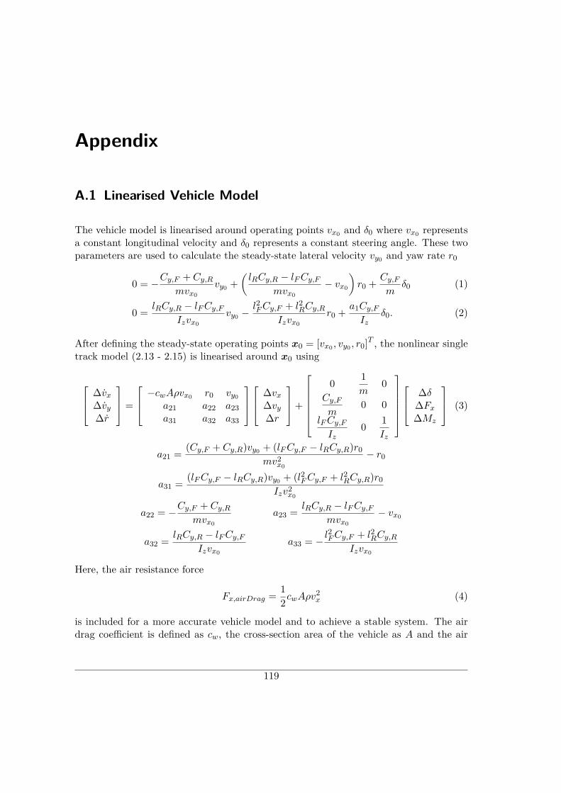
Appendix
A.1 Linearised Vehicle Model
The vehicle model is linearised around operating points vx0 and δ0 where vx0 representsa constant longitudinal velocity and δ0 represents a constant steering angle. These twoparameters are used to calculate the steady-state lateral velocity vy0 and yaw rate r0
0 = −Cy,F + Cy,Rmvx0
vy0 +(lRCy,R − lFCy,F
mvx0− vx0
)r0 + Cy,F
mδ0 (1)
0 = lRCy,R − lFCy,FIzvx0
vy0 −l2FCy,F + l2RCy,R
Izvx0r0 + a1Cy,F
Izδ0. (2)
After defining the steady-state operating points x0 = [vx0 , vy0 , r0]T , the nonlinear singletrack model (2.13 - 2.15) is linearised around x0 using
∆vx∆vy∆r
=
−cwAρvx0 r0 vy0
a21 a22 a23a31 a32 a33
∆vx
∆vy∆r
+
0 1
m0
Cy,Fm
0 0lFCy,FIz
0 1Iz
∆δ
∆Fx∆Mz
(3)
a21 = (Cy,F + Cy,R)vy0 + (lFCy,F − lRCy,R)r0mv2
x0
− r0
a31 = (lFCy,F − lRCy,R)vy0 + (l2FCy,F + l2RCy,R)r0Izv2
x0
a22 = −Cy,F + Cy,Rmvx0
a23 = lRCy,R − lFCy,Fmvx0
− vx0
a32 = lRCy,R − lFCy,FIzvx0
a33 = − l2FCy,F + l2RCy,R
Izvx0
Here, the air resistance force
Fx,airDrag = 12cwAρv
2x (4)
is included for a more accurate vehicle model and to achieve a stable system. The airdrag coefficient is defined as cw, the cross-section area of the vehicle as A and the air
119
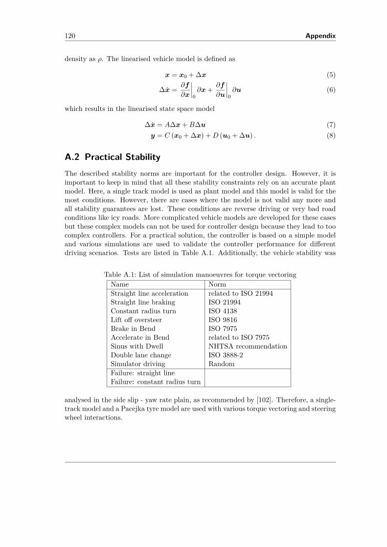
120 Appendix
density as ρ. The linearised vehicle model is defined as
x = x0 + ∆x (5)
∆x = ∂f
∂x
∣∣∣∣0∂x+ ∂f
∂u
∣∣∣∣0∂u (6)
which results in the linearised state space model
∆x = A∆x+B∆u (7)y = C (x0 + ∆x) +D (u0 + ∆u) . (8)
A.2 Practical StabilityThe described stability norms are important for the controller design. However, it isimportant to keep in mind that all these stability constraints rely on an accurate plantmodel. Here, a single track model is used as plant model and this model is valid for themost conditions. However, there are cases where the model is not valid any more andall stability guarantees are lost. These conditions are reverse driving or very bad roadconditions like icy roads. More complicated vehicle models are developed for these casesbut these complex models can not be used for controller design because they lead to toocomplex controllers. For a practical solution, the controller is based on a simple modeland various simulations are used to validate the controller performance for differentdriving scenarios. Tests are listed in Table A.1. Additionally, the vehicle stability was
Table A.1: List of simulation manoeuvres for torque vectoringName NormStraight line acceleration related to ISO 21994Straight line braking ISO 21994Constant radius turn ISO 4138Lift off oversteer ISO 9816Brake in Bend ISO 7975Accelerate in Bend related to ISO 7975Sinus with Dwell NHTSA recommendationDouble lane change ISO 3888-2Simulator driving RandomFailure: straight lineFailure: constant radius turn
analysed in the side slip - yaw rate plain, as recommended by [102]. Therefore, a single-track model and a Pacejka tyre model are used with various torque vectoring and steeringwheel interactions.
Bibliography
[1] J. Lee, Beijing slashes car sales quota in anti-pollution drive. Reuters, 28March 2014. [Online]. Available: http://www.reuters.com/article/2013/11/05/us-china-cars-idUSBRE9A40AP20131105
[2] B. Love and M. John, Police sent to enforce car ban as Paris battles smog.Reuters, 28 March 2014. [Online]. Available: http://www.reuters.com/article/2014/03/17/france-pollution-idUSL6N0ME1NV20140317
[3] D. Rutherford, Hybrids break through in the Japan auto market. InternationalCouncil on Clean Transportation, 4 April 2014. [Online]. Available: http://www.theicct.org/blogs/staff/hybrids-break-through-japan-auto-market
[4] K. McPhaul, “California Auto Outlook,” California Auto Outlook Market Report,vol. 9, no. 3, pp. 1–6, 2013.
[5] T. Bosa and A. Vartmann, Weltweit ueber 400.000 Elektroautos unterwegs.Zentrum fuer Sonnenenergie und Wasserstoff-Forschung Baden-Wuerttemberg,31 March 2014. [Online]. Available: http://www.zsw-bw.de/uploads/media/pi04-2014-ZSW-StandElektromobilitaetweltweit.pdf
[6] P. Mock and Z. Yang, “Driving Electrification - a Global Comparison of FiscalIncentive Policy for Electric Vehicles,” White Paper, 5 May 2014. [Online].Available: www.theicct.org
[7] F. Carranza, O. Paturet, and S. Salera, “Norway, the most successful market forElectric Vehicles,” in Proceedings of the Electric Vehicle Symposium, Barcelona,Spain, 2013, pp. 1–6.
[8] L. Eckstein, R. Goebbels, and R. Wohlecker, “Benchmarking of the Electric VehicleMitsubishi I-Miev,” ATZautotechnology, vol. 11, no. 6, pp. 26–33, 2011.
[9] B. Wang, M. Li, M. Xu, and J. Zhou, “Simulation-Based Energy Flow Study ofPurely Electric-Drive Vehicles,” in Proceedings of the FISITA 2012 World Auto-motive Congress, Beijing, China, 2012, pp. 615–630.
[10] R. Garcia-Valle, Electric Vehicle Integration into Modern Power Networks.Springer, 2013.
[11] Volvo, C30 Electric. Volvo Car Corporation, 22 May 2014. [Online]. Available:http://www.volvocars.com/intl/campaigns/electric/Pages/default.aspx
121
122 Bibliography
[12] M. Jung, F. Kessler, P. Mueller, and S. Wahl, “Vehicle Integration and DrivingCharacteristics of the BMW Active E,” ATZ worldwide, vol. 114, no. 10, pp. 52–56,2012.
[13] Plugincars, 2014 Toyota RAV4 EV. PluginCars.com, 22 May 2014. [Online].Available: http://www.plugincars.com/toyota-rav4-ev-new
[14] Chevrolet, Spark EV. General Motors, 22 May 2014. [Online]. Available:http://www.chevrolet.com/spark-ev-electric-vehicle.html
[15] R. Lane, Honda Fit EV axed: Is this proof Honda sees no future in electric cars?ecomento UG, 28 February 2014. [Online]. Available: http://ecomento.com/2014/02/28/honda-fit-ev-axed-proof-honda-sees-future-electric-cars/
[16] J. Feustel, S. Lang, and M. Hand, “The Electric Super Sports Car SLS AMGElectric Drive,” ATZ worldwide eMagazines, vol. 115, no. 01, pp. 4–10, 2013.
[17] S. Siler, Mitsubishi i MiEV Sport Concept. Hearst Communications, Inc.,31 October 2007. [Online]. Available: http://www.caranddriver.com/news/mitsubishi-i-miev-sport-concept-auto-shows
[18] L. Kingston, Audi R8 e-tron review. Haymarket Media Group Limited, 22 May2014. [Online]. Available: http://www.autocar.co.uk/car-review/audi/r8-e-tron
[19] Rimac, Concept One - Torque Vectoring. Rimac Automobili, 31 December2012. [Online]. Available: http://www.rimac-automobili.com/concept_one/torque-vectoring-7
[20] eFuture, Efficient Mobility. European Community Seventh Framework Prgramme(FP7/2007-2013) under grant agreement No.258133, 31 October 2013. [Online].Available: http://www.efuture-eu.org
[21] K. Roebuck, AUTOSAR - AUTomotive Open System ARchitecture. Emereo Pub-lishing, 2012.
[22] Norm, Road vehicles – Functional safety. ISO, Geneva, Switzerland, 2011, no.ISO 26262-1:2011.
[23] S. Skogestad and I. Postlethwaite, Multivariable feedback control analysis and de-sign, 2nd ed. Wiley-Interscience, 2005.
[24] Norm, Road vehicles – Vehicle dynamics and road-holding ability – Vocabulary.ISO, Geneva, Switzerland, 1991, no. ISO 8855:1991.
[25] R. N. Jazar, Vehicle Dynamics - Theory and Application. Springer, 2008.
[26] B. A. Guvenc, T. Acarman, and L. Guvenc, “Coordination of steering and indi-vidual wheel braking actuated vehicle yaw stability control,” in Proceedings of theIntelligent Vehicles Symposium, Columbus, Ohio, USA, 2003, pp. 288–293.
Bibliography 123
[27] R. J. Rieveley and B. P. Minaker, “Variable Torque Distribution Yaw MomentControl for Hybrid Powertrains,” in SAE Technical Paper 2007-01-0278. Societyof Automotive Engineers, Inc., 2007.
[28] C. Zhao, W. Xiang, and P. Richardson, “Vehicle Lateral Control and Yaw StabilityControl through Differential Braking,” in Proceedings of the IEEE InternationalSymposium on Industrial Electronics, Montreal, Canada, 2006, pp. 384–389.
[29] A. Rucco, G. Notarstefano, and J. Hauser, “Dynamics exploration of a single-track rigid car model with load transfer,” in Proceedings of the IEEE Conferenceon Decision and Control, Atlanta, Georgia, USA, 2010, pp. 4934–4939.
[30] L. Menhour, D. Lechner, and A. Chara, “Sliding mode control to design a drivermodel for vehicle steering: Experimental validation and stability evaluation ofsideslip motion,” in Proceedings of the IFAC Symposium Advances in AutomotiveControl, Munich, Germany, 2010, pp. 7–12.
[31] Y.-H. J. Hsu and J. C. Gerdes, “Stabilization of a steer-by-wire vehicle at thelimits of handling using feedback linearization,” in Proceedings of the ASME In-ternational Mechanical Engineering Congress and Exposition, Orlando, Floriada,USA, 2005, pp. 1–10.
[32] D. V. T. Truong and W. Tomaske, “Active front steering system using adaptivesliding mode control,” in Proceedigns of the Chinese Control and Decision Confer-ence, Guiyang, China, 2013, pp. 253–258.
[33] S. Anwar, “Yaw Stability Control of an Automotive Vehicle via Generalized Pre-dictive Algorithm,” in Proceedings of the American Control Conference, Portland,Oregon, USA, 2005, pp. 435–440.
[34] L. Xiong, Z. Yu, and Y. Meng, “Vehicle dynamic control for a 4 in-wheel-motoredEV based on identification of tyre cornering stiffness,” in Proceedings of the Inter-national Symposium on Advanced Vehicle Control, Loughborough, UK, 2010, pp.861–866.
[35] Robert Bosch GmbH, Bosch Automotive Handbook, 8th ed. Wiley, 2007.
[36] H. B. Pacejka, Tyre and Vehicle Dynamics. Elsevier, 2006.
[37] H. Dugoff, P. S. Fancher, and L. Segel, “An Analysis of Tire Traction Propertiesand Their Influence on Vehicle Dynamic Performance,” in SAE Technical Paper700377. Society of Automotive Engineers, Inc., 1970.
[38] Z. Shiller, “Optimization Tools for Automated Vehicle Systems,” in UC Berkeley:California Partners for Advanced Transit and Highways (PATH), 1995, pp. 1–29.
[39] D. Schramm, M. Hiller, and R. Bardini, Modellbildung und Simulation der Dy-namik von Kraftfahrzeugen. Springer, 2010.
124 Bibliography
[40] E. Bakker, L. Nyborg, and H. B. Pacejka, “Tyre Modelling for Use in VehicleDynamic Studies,” in SAE Technical Paper 870421. Society of Automotive En-gineers, Inc., 1987.
[41] Corrsys Datron, Correvit sensor. Sensorsysteme GmbH, 04 December2012. [Online]. Available: http://www.corrsys-datron.com/Support/Manuals/Bedienungsanleitungen/a_Sensoren/cds-m_L-400_d.pdf
[42] Norm, Passenger cars – Test track for a severe lane-change manoeuvre – Part 2:Obstacle avoidance. ISO, Geneva, Switzerland, 2002, no. ISO 3888-2:2002.
[43] F. Braghin and E. Sabbioni, “Development of a control strategy for improving ve-hicle safety in a hybrid vehicle with four independently driven in-wheel motors,” inProceedings of the International Symposium on Advanced Vehicle Control, Lough-borough, UK, 2010, pp. 91–96.
[44] Y. Gan, L. Xiong, and F. Martinez, “A Torque Vectoring Control System forManeuverability Improvement of 4WD EV,” in Proceedings of the InternationalConference on Computer Science and Electronics Engineering, Hangzhou, China,2013, pp. 2729–2732.
[45] K. Sawase and K. Inoue, “Maximum acceptable differential speed ratio of lateraltorque-vectoring differentials for vehicles,” Journal of Automobile Engineering, vol.223, no. 8, pp. 967–978, 2009.
[46] J. Wang, Q. Wang, C. Song, L. Chu, and Y. Wang, “Coordinated control of differ-ential drive assisted steering system with vehicle stability enhancement system,” inProceedings of the Intelligent Vehicles Symposium, Baden-Baden, Germany, 2011,pp. 1148 –1155.
[47] L. De Novellis, A. Sorniotti, P. Gruber, L. Shead, V. Ivanov, and K. Hoep-ping, “Torque Vectoring for Electric Vehicles with Individually Controlled Motors:State-of-the-Art and Future Developments,” in Proceedings of the Electric VehicleSymposium, Los Angeles, California, USA, 2012, pp. 1–12.
[48] L. De Novellis, A. Sorniotti, and P. Gruber, “Wheel Torque Distribution Criteriafor Electric Vehicles With Torque-Vectoring Differentials,” IEEE Transactions onVehicular Technology, vol. 63, no. 4, pp. 1593–1602, 2013.
[49] V. Ivanov, K. Augsburg, and D. Savitski, “Torque Vectoring for Improving theMobility of All-Terrain Electric Vehicles,” in Proceedings of the European Re-gional Conference of the International Society for Terrain-Vehicle-Systems, Pre-toria, South Africa, 2012, pp. 1–8.
[50] S. Fallah, A. Khajepour, B. Fidan, S.-K. Chen, and B. Litkouhi, “Vehicle OptimalTorque Vectoring Using State-Derivative Feedback and Linear Matrix Inequality,”IEEE Transactions on Vehicular Technology, vol. 62, no. 4, pp. 1540–1552, 2013.
Bibliography 125
[51] A. T. Van Zanten, “Evolution of electronic control systems for improving the vehi-cle dynamic behavior,” in Proceedings of the International Symposium on AdvancedVehicle Control, Hiroshima, Japan, 2002, pp. 1–9.
[52] U. Kiencke and L. Nielsen, Automotive Control Systems - For Engine, Driveline,and Vehicle. Springer, 2005.
[53] D. Schuring, W. Pelz, and M. G. a. Pottinger, “A Model for Combined Tire Corner-ing and Braking Forces,” in SAE Technical Paper 960180. Society of AutomotiveEngineers, Inc., 1996.
[54] R. Peter, C. Granzow, M. Spieß, and R. Denzler, “The vector drive rear axletransmission,” ATZ worldwide, vol. 109, no. 12, pp. 2–5, 2007.
[55] M. Lehmann and J. Schuller, “Validation of safety limits for an electrical drivesystem with variable torque distributions,” in Proceedings of Der Fahrer im 21Jahrhundert, Braunschweig, Germany, 2013, pp. 1–12.
[56] W. Weber, Fahrdynamik in Perfektion - der Weg zum optimalen Fahrwerk-Setup,2nd ed. Motorbuch-Verl, 2011.
[57] Y. Shibahata and T. Tomari, “Direct Yaw Control Torque Vectoring,” AutoTech-nology, vol. 6, no. 3, pp. 34–38, 2006.
[58] K.-W. Huenermann, S. Enzinger, T. WilK, and K. Volkmar, “Electronic stabilisa-tion program ESP,” ATZextra worldwide, vol. 15, no. 11, pp. 106–111, 2010.
[59] C. Billig, H. Boedrich, J. Brack, B. Hoell, M. Holle, and F. Kimmich, “The dynamicperformance control from BMW,” ATZ worldwide, vol. 110, no. 11, pp. 19–25, 2008.
[60] Daimler, Mercedes-Benz S 63 AMG and S 65 AMG. Daimler AG, 15 June 2009.[Online]. Available: http://media.daimler.com/Projects/c2c/channel/documents/1721159_PM_S_63_S_65_AMG_en.pdf
[61] Mitsubishi, Outlander. MNM Media LLC, 22 May 2014. [Online]. Available:http://www.leftlanenews.com/new-car-buying/mitsubishi/outlander/
[62] P. Schaefer, G. Wahl, and M. Harrer, “The chassis of the Porsche 911,” ATZworldwide, vol. 114, no. 6, pp. 4–8, 2012.
[63] Daimler, Torque Vectoring Brake. Daimler AG, 22 May 2014. [Online]. Available:http://techcenter.mercedes-benz.com/en/torque_vectoring_brake/detail.html
[64] McLaren, Formula 1 technology delivers ultimate performance on track and roadin the new MP4-12C. McLaren Automotive Limited, 4 November 2011. [Online].Available: http://media.mclarenautomotive.com/release/109
[65] Ford, Torque Vectoring Control. Ford-Werke GmbH, 22 May 2014. [Online]. Avail-able: http://www.ford.de/FordTechnologien/Qualitaet/mdp=v1204985020885
126 Bibliography
[66] Nissan, Torque Vectoring All-wheel drive. Nissan USA, 22 May 2014.[Online]. Available: http://www.nissanusa.com/buildyournissan/vehicle-images/2013/JKE/XGC30NIS122B0/68a73b82a34f478e7e29e2f9ce99c6c6/JUKE/SV/Torque-Vectoring-All-wheel-drive/Performance
[67] G. McGovern, Range Rover Sport Specification. Jaguar Land Rover Limited, 31December 2013. [Online]. Available: http://www.landrover.com/content/us/pdf/l494-pdf
[68] HSV, Torque Vectoring. Holden Special Vehicles, 22 May 2014. [Online].Available: http://www.hsv.com.au/Gen-F/feel/performance-technology/
[69] Cadillac, 2014 XTS SEDAN. General Motors, 22 May 2014. [Online]. Available:http://www.cadillac.com/xts-luxury-sedan/features-specs/models.html
[70] Toyota, New Lexus RC F combines Aggressive Stylingwith high Performance. Toyota Motor Corporation, 14 Jan-uary 2014. [Online]. Available: http://www.lexus-int.com/news/new-lexus-rc-f-combines-aggressive-styling-with-high-performance.html
[71] L. Palladino, G. Duc, and R. Pothin, “LPV control of a road vehicle during brakingaction in curve,” in Proceedings of the IFAC Symposium on Robust Control Design,Toulouse, France, 2006, pp. 113–118.
[72] C. S. Baslamish, I. E. Kose, and G. Anlas, “Design of active steering and intel-ligent braking systems for road vehicle handling improvement: A robust controlapproach,” in Proceedings of the IEEE International Conference on Control Ap-plications, Munich, Germany, 2006, pp. 909–914.
[73] M. Doumiati, O. Sename, L. Dugard, J.-J. Martinez-Molina, P. Gaspar, and Z. Sz-abo, “Integrated vehicle dynamics control via coordination of active front steeringand rear braking,” European Journal of Control, vol. 19, no. 2, pp. 121 – 143, 2013.
[74] S. Di Cairano, H. E. Tseng, D. Bernardini, and A. Bemporad, “Vehicle Yaw Stabil-ity Control by Coordinated Active Front Steering and Differential Braking in theTire Sideslip Angles Domain,” IEEE Transactions on Control Systems Technology,vol. 21, no. 4, pp. 1236–1248, 2013.
[75] R. Rajamani and D. Piyabongkarn, “New paradigms for the integration of yaw sta-bility and rollover prevention functions in vehicle stability control,” IEEE Trans-actions on Intelligent Transportation Systems, vol. 14, no. 1, pp. 249–261, 2013.
[76] D. Piyabongkarn, J. Grogg, Q. Yuan, J. Lew, and R. Rajamani, “Dynamic Mod-eling of Torque-Biasing Devices for Vehicle Yaw Control,” in Proceedings of theAutomotive Dynamics, Stability and Controls Conference and Exhibition, Novi,Michigan, USA, 2006.
Bibliography 127
[77] C. Poussot-Vassal, O. Sename, L. Dugard, and S. M. Savaresi, “Vehicle dynamicstability improvements through gain-scheduled steering and braking control,” Ve-hicle System Dynamics, vol. 49, no. 10, pp. 1597–1621, 2011.
[78] L. De Novellis, A. Sorniotti, P. Gruber, and A. Pennycott, “Comparison of Feed-back Control Techniques for Torque-Vectoring Control of Fully Electric Vehicles,”IEEE Transaction on Vehicular Technology (early access article), vol. PP, no. 99,pp. 1–12, 2014.
[79] Q. Liu, G. Kaiser, S. Boonto, H. Werner, F. Holzmann, B. Chretien, and M. Ko-rte, “Two-Degree-of-Freedom LPV Control for a through-the-Road Hybrid ElectricVehicle via Torque Vectoring,” in Proceedings of the IEEE Conference on Decisionand Control and European Control Conference, Orlando, Florida, USA, 2011, pp.1274 – 1279.
[80] L. Pinto, S. Aldworth, M. Watkinson, P. Jeary, and M. Franco-Jorge, “AdvancedYaw Motion Control of a Hybrid Vehicle using Twin Rear Electric Motors,” inProceedings of the International Symposium on Advanced Vehicle Control, Lough-borough, UK, 2010, pp. 640–645.
[81] M. Milehins, C. Cheng, T.-W. Chu, and R. P. Jones, “Handling behaviour of a TTRhybrid electric vehicle with independent rear wheel torque control,” in Proceedingsof the International Symposium on Advanced Vehicle Control, Loughborough, UK,2010, pp. 556–561.
[82] R. Mario and S. Scalzi, “Integrated Active Front Steering and Semiactive RearDifferential Control in Rear Wheel Drive Vehicles,” in Proceedings of the WorldCongress International Federation of Automatic Control, Seoul, Korea, 2008, pp.10 732–10 737.
[83] D. Zhang, G. Liu, L. Wang, P. Miao, G. Sun, and H. Zhou, “Active Safety Neu-ral Network Inverse Decoupling Control for Multi-Wheel Independently DrivenElectric Vehicles,” in Proceedings of the IEEE Vehicle Power and Propulsion Con-ference, Beijing, China, 2013, pp. 45–48.
[84] W. Chu, Y. Luo, Y. Dai, and K. Li, “Traction system coordinated allocationcontrol for four wheel independently driven electric vehicle,” in Proceedings of theInternational Symposium on Advanced Vehicle Control, Seoul, Korea, 2012, pp.1–6.
[85] J. Song, J. Hwang, and K. Bae, “Design and Evaluation of an Integrated Con-trolof AFS and DYC Systems,” in Proceedings of the International Symposium onAdvanced Vehicle Control, Seoul, Korea, 2012, pp. 1–6.
[86] D. Rubin and S. Arogeti, “Vehicle yaw stability control using rear active differentialvia Sliding mode control methods,” in Proceedings of the Mediterranean Conferenceon Control Automation, Platanias-Chania, Greece, 2013, pp. 317–322.
128 Bibliography
[87] A. Tavasoli and M. Naraghi, “Comparison of static and dynamic control alloca-tion techniques for integrated vehicle control,” in Proceedings of the IFAC WorldCongress of the International Federation of Automatic Control, Milano, Italy, 2011,pp. 7180–7185.
[88] G. Kaiser, F. Holzmann, B. Chretien, M. Korte, and H. Werner, “Torque Vectoringwith a feedback and feed forward controller - applied to a through the road hybridelectric vehicle,” in Proceedings of the Intelligent Vehicles Symposium, Baden-Baden, Germany, 2011, pp. 448–453.
[89] C. Geng, L. Mostefai, D. Mouloud, and Y. Hori, “Direct Yaw-Moment Control ofan In-Wheel-Motored Electric Vehicle Based on Body Slip Angle Fuzzy Observer,”IEEE Transactions on Industrial Electronics, vol. 56, no. 5, pp. 1411–1419, 2009.
[90] L. Chu, M. Xu, Y. Zhang, Y. Ou, and Y. Shi, “Vehicle Dynamics Control Based onOptimal Sliding Mode Control Theory,” in Proceedings of the International Confer-ence on Computer, Mechatronics, Control and Electronic Engineering, Changchun,China, 2010, pp. 486–491.
[91] I. Yang, S. Byun, B. Seo, D. Lee, and D. S. Han, “Integrated control systemsof active front steering and direct yaw moment control using dynamic inversion,”in Proceedings of the Intelligent Vehicles Symposium, Gold Coast City, Australia,2013, pp. 1303–1306.
[92] L. Wang, G. Liu, D. Zhang, and P. Miao, “Integrated control of active front steeringand direct yaw moment for multi-wheel independently driven electric vehicles,” inProceedings of the International Conference on Electrical Machines and Systems,Busan, Korea, 2013, pp. 2301–2304.
[93] S. Kaspar, A. Pruckner, S. Ralf, and H. Soeren, “Potential of Vehicle Dynamicsvia Single Wheel Drive for Installation Space Optimized Electric Vehicles,” inProceedings of the Aachen Colloquium Automobile and Engine Technology, Aachen,Germany, 2012, pp. 675–698.
[94] S. Kaspar, R. Stroph, T. Buente, and S. Hohmann, “Optimisation of vehicle dy-namics via torque vectoring for space optimised electric vehicles,” ATZ worldwide,vol. 116, no. 2, pp. 54–60, 2014.
[95] G. J. Silva, S. P. Bhattachaiyya, and A. Datta, PID Controllers for Time-DelaySystems. Birkhaeuser, 2005.
[96] T. Armstrong, W. Manning, I. Hogan, and A. Shenfield, “Vehicle Dynamics Con-trol in Hybrid Electric Vehicles,” in Proceedings of the International Symposiumon Advanced Vehicle Control, Loughborough, UK, 2010, pp. 1–6.
[97] J. Lee and H. Koo, “Linear Handling Performance Improvement of Passenger Vehi-cle using Torque Vectoring System,” in Proceedings of the International Symposiumon Advanced Vehicle Control, Seoul, Korea, 2012, pp. 1–6.
Bibliography 129
[98] J.-E. Moseberg and G. Roppenecker, “Steuerung und Regelung der horizontalenFahrzeugbewegung mit Einzelradaktorik,” at - Automatisierungstechnik, vol. 62,no. 3, pp. 216–225, 2013.
[99] S. Hillenbrand and I. Stolpe, “Optimization of Tire Friction Usage by Active Driv-ing Torque Distribution,” at - Automatisierungstechnik, vol. 57, no. 5, pp. 223–229,2009.
[100] P. He and Y. Hori, “Optimum traction force distribution for stability improvementof 4WD EV in critical driving condition,” in Proceedings of the IEEE InternationalWorkshop on Advanced Motion Control, Istambul, Turkey, 2006, pp. 596–601.
[101] M. Canale, L. Fagiano, M. Milanese, and P. Borodani, “Robust vehicle yaw controlusing active differential and internal model control techniques,” in Proceedings ofthe American Control Conference, Minneapolis, Minnesota, USA, June 2006, pp.5354–5359.
[102] E. Ono, S. Hosoe, H. D. Tuan, and S. Doi, “Bifurcation in vehicle dynamics androbust front wheel steering control,” IEEE Transactions on Control Systems Tech-nology, vol. 6, no. 3, pp. 412–420, 1998.
[103] C. Poussot-Vassal, “Robust multivariable linear parameter varying automotiveglobal chassis control,” Ph.D. dissertation, Grenoble INP, France, 2008.
[104] S. C. a. Baslamish, “LPV Modeling and Robust Control of Yaw and Roll Modesof Road Vehicles,” Ph.D. dissertation, Bogazici University, Turkey, 2007.
[105] L. Palladino, G. Duc, and R. Pothin, “LPV Control for mu-split braking assistanceof a road vehicle,” in Proceedings of the IEEE Conference on Decision and Controland European Control Conference, Seville Spain, 2005, pp. 2664–2669.
[106] G. Kaiser, Q. Liu, C. Hoffmann, M. Korte, and H. Werner, “Torque vectoring foran electric vehicle using an LPV drive controller and a torque and slip limiter,”in Proceedings of the IEEE Conference on Decision and Control, Maui, Hawaii,USA, 2012, pp. 5016–5021.
[107] G. Kaiser, M. Korte, Q. Liu, C. Hoffmann, and H. Werner, “Torque Vectoring fora Real, Electric Car Implementing an LPV Controller,” in Proceedings of the IFACWorld Congress of the International Federation of Automatic Control, CapeTown,South Africa, 2014.
[108] M. Bartels, Q. Liu, G. Kaiser, and H. Werner, “LPV Torque Vectoring for anElectric Vehicle - Using Parameter-Dependent Lyapunov Functions,” in AmericanControl Conference, 2013, pp. 2156–2161.
[109] A. Emami-Naeini and P. Van Dooren, “Computation of Zeros of Linear Multivari-able Systems,” Automatica, vol. 18, no. 4, pp. 415–430, 1982.
130 Bibliography
[110] D. Liberzon and A. S. Morse, “Basic problems in stability and design of switchedsystems,” IEEE Control Systems Magazine, vol. 19, no. 5, pp. 59–70, 1999.
[111] J. Loefberg, “YALMIP: A toolbox for modeling and optimization in Matlab,” inProceedings of the IEEE International Symposium on Computer Aided ControlSystems Design, Taipei, Taiwan, 2004, pp. 284–289.
[112] MATLAB, version 7.12.0 (R2011b). Natick, Massachusetts: The MathWorksInc., 2011.
[113] M. Chilali and P. Gahinet, “H-infinity design with pole placement constraints:an LMI approach,” IEEE Transactions on Automatic Control, vol. 41, no. 3, pp.358–367, 1996.
[114] P. Apkarian, G. Becker, P. Gahinet, and H. Kajiwara, LMI Techniques in ControlEngineering from Theory to Practice -, Kobe, Japan, 1996.
[115] S. Lim, “Analysis and Control of Linear Parameter-Varying Systems,” Ph.D. dis-sertation, Stanford University, Standford, California, USA, 1999.
[116] S. P. Boyd, L. El Ghaoui, E. Feron, and V. Balakrishnan, Linear matrix inequalitiesin system and control theory. SIAM, 1994, vol. 15.
[117] A. M. Lyapunov, “A general task about the stability of motion,” Ph.D. dissertation,Kharkov Mathematical Society, University of Kharkov, Ukrain, 1892.
[118] A. J. van der Schaft, “L2-gain analysis of nonlinear systems and nonlinear state-feedback H∞; control,” IEEE Transactions on Automatic Control, vol. 37, no. 6,pp. 770–784, 1992.
[119] A. Varga, A. Hansson, and P. Guilhem, Optimization based clearance of flightcontrol laws - A civil aircraft application. Springer, 2012.
[120] A. S. Ghersin and R. S. S. Pena, “LPV control of a 6-DOF vehicle,” IEEE Trans-actions on Control Systems Technology, vol. 10, no. 6, pp. 883–887, 2002.
[121] B. Lu, F. Wu, and S. Kim, “Switching LPV control of an F-16 aircraft via controllerstate reset,” IEEE Transactions on Control Systems Technology, vol. 14, no. 2, pp.267–277, 2006.
[122] Q. Chu, B. Mulder, D. Choukroun, E.-J. v. Kampen, C. d. Visser, and G. Looye,Advances in aerospace guidance, navigation and control. Springer, 2013.
[123] Z. Yu, H. Chen, and P.-y. Woo, “Gain scheduled LPV H-infty control based onLMI approach for a robotic manipulator,” Journal of Robotic Systems, vol. 19,no. 12, pp. 585–593, 2002.
Bibliography 131
[124] F. Saupe and H. Pfifer, “Applied LPV control exploiting the separation principlefor the single axis positioning of an industrial manipulator,” in Proceedings of theIEEE International Conference on Control Applications, Denver, Colorado, USA,2011, pp. 1476–1481.
[125] S. M. Hashemi, H. S. Abbas, and H. Werner, “LPV modelling and control of a2-DOF robotic manipulator using PCA-based parameter set mapping,” in Pro-ceedings of the IEEE Conference on Decision and Control, Shanghai, China, 2009,pp. 7418–7423.
[126] M. Corno, S. M. Savaresi, and G. J. Balas, “On linear-parameter-varying (LPV)slip-controller design for two-wheeled vehicles,” International Journal of Robustand Nonlinear Control, vol. 19, no. 12, pp. 1313–1336, 2009.
[127] A.-L. Do, O. Sename, and L. Dugard, “An LPV control approach for semi-activesuspension control with actuator constraints,” in Proceedings of the American Con-trol Conference, Baltimore, Maryland, USA, 2010, pp. 4653–4658.
[128] A. Kwiatkowski, J. P. Blath, H. Werner, and M. Schultalbers, “Application of LPVgain scheduling to charge control of a SI engine,” in Proceedings of the IEEE In-ternational Symposium on Intelligent Control, Munich, Germany, 2006, pp. 2327–2331.
[129] P. Apkarian, P. Gahinet, and G. Becker, “Self-scheduled Hinf Control of LinearParameter-Varying Systems: a Design Example,” Automatica, vol. 31, no. 9, pp.1251–1261, 1995.
[130] A. Kwiatkowski and H. Werner, “PCA-Based Parameter Set Mappings for LPVModels With Fewer Parameters and Less Overbounding,” IEEE Transactions onControl Systems Technology, vol. 16, no. 4, pp. 781–788, 2008.
[131] P. Apkarian and P. Gahinet, “A convex characterization of gain-scheduled H∞controllers,” IEEE Transactions on Automatic Control, vol. 40, no. 5, pp. 853–864, 1995.
[132] C. W. Scherer, “LPV control and full block multipliers,” Automatica, vol. 37, no. 3,pp. 361–375, 2001.
[133] F. Wu and K. Dong, “Gain-scheduling control of LFT systems using parameter-dependent Lyapunov functions,” Automatica, vol. 42, no. 1, pp. 39–50, 2006.
[134] A. Kwiatkowski, “LPV Modeling and Appliction of LPV Controllers to SI En-gines,” Ph.D. dissertation, Technical University - Hambur Harburg, Germany,2007.
[135] D. C. McFarlane and K. Glover, Robust Controller Design Using Normalized Co-prime Factor Plant Descriptions. Springer, 1990.
132 Bibliography
[136] D. Bates and M. Hagstroem, Nonlinear Analysis and Synthesis Techniques forAircraft Control. Springer, 2009.
[137] H. H. Bauschke, Fixed-Point Algorithms for Inverse Problems in Science and En-gineering. Springer, 2011.
[138] J. M. Barker and G. J. Balas, “Comparing linear parameter-varying gain-scheduledcontrol techniques for active flutter suppression,” Journal of Guidance, Control andDynamics, vol. 23, no. 5, pp. 948–955, 2000.
[139] C. Hoffmann and H. Werner, “A Survey of Linear Parameter-Varying Control Ap-plications Validated by Experiments or High-Fidelity Simulations,” IEEE Trans-actions on Control Systems Technology (early access article), vol. PP, no. 99, pp.1–1, 2014.
[140] ——, “Complexity of Implementation and Synthesis in Linear Parameter-VaryingControl,” in Proceeding of the IFAC World Congress International Federation ofAutomatic Control, Cape Town, South Africa, 2014.
[141] C. Hoffmann, S. M. Hashemi, H. S. Abbas, and H. Werner, “Synthesis of LPV Con-trollers with Reduced Implementation Complexity,” in Proceedings of the AmericanControl Conference, Portland, Oregon, USA, 2014.
[142] S. Tarbouriech and M. C. Turner, “Anti-windup design: an overview of some recentadvances and open problems,” IET Control Theory Applications, vol. 3, no. 1, pp.1–19, 2009.
[143] G. Stein, “Respect the unstable,” IEEE Control Systems, vol. 23, no. 4, pp. 12–25,2003.
[144] A. Visioli, Practical PID Control. Springer, 2006.
[145] M. C. Turner and D. G. Bates, Mathematical Methods for Robust and NonlinearControl. New York: Springer, 2007.
[146] S. Tarbouriech, G. Garcia, and A. H. Glattfelder, Advanced Strategies in ControlSystems with Input and Output Constraints. Springer, 2007.
[147] J. Oehr, “Anti-windup and Control of Systems with Multiple Input Saturations -Tools, Solutions and Case Studies,” Ph.D. dissertation, Uppsala University, 2003.
[148] M. C. Turner and I. Postlethwaite, “A new perspective on static and low orderanti-windup synthesis,” International Journal of Control, vol. 77, no. 1, pp. 27–44,2004.
[149] P. F. Weston and I. Postlethwaite, “Linear conditioning for systems containingsaturating actuators,” Automatica, vol. 36, no. 9, pp. 1347–1354, 2000.
Bibliography 133
[150] WIVW, Driving Simulator. Wuerzburg Institute for Traffic Sciences GmbH, 31October 2013. [Online]. Available: www.wivw.de
[151] R. Isermann, Fahrdynamik-Regelung - Modellbildung, Fahrerassistenzsysteme,Mechatronik. Vieweg und Sohn, 2006.
[152] J. G. Brookshear and D. T. Smith, Computer science - an overview, 11th ed.Addison-Wesley, 2012.
[153] Norm, Passenger cars – Stopping distance at straight-line braking with ABS –Open-loop test method. ISO, Geneva, Switzerland, 2007, no. ISO 21994:2007.
[154] ——, Passengers cars – Steady-state circular driving behaviour – Open-loop testmethods. ISO, Geneva, Switzerland, 2004, no. ISO 4138:2004.
[155] ——, Passenger cars – Braking in a turn – Open-loop test method. ISO, Geneva,Switzerland, 2006, no. ISO 7975:2006.
[156] ——, Passenger cars – Power-off reaction of a vehicle in a turn – Open-loop testmethod. ISO, Geneva, Switzerland, 2006, no. ISO 9816:2006.
[157] G. J. Forkenbrock, “An Overview of NHTSA’s ESC Research Program,” in Na-tional Highway Traffic Safety Administration, 2005.
[158] G. Genta, F. F. Ling, and L. Morello, The Automotive Chassis - Vol. 1: Compo-nents Design. Springer, 2009.
[159] M. Trzesniowski, Rennwagentechnik - Grundlagen, Konstruktion, Komponenten,Systeme. Vieweg+Teubner, 2008.
[160] R. Rajamani, Vehicle Dynamics and Control, 2nd ed. Springer, 2006.
[161] K. J. Astroem and B. Wittenmark, Computer controlled systems - theory anddesign, 3rd ed. Prentice Hall, 1997.
[162] J. Lunze, Regelungstechnik 2 - Mehrgroessensysteme, Digitale Regelung, 6th ed.Springer, 2010.
[163] F. Haugen, Discrete-time signals and systems. TechTeach, 2005.
[164] R. Toth, P. S. C. Heuberger, and P. M. J. van den Hof, “Discretisation of linearparameter-varying state-space representations,” IET Control Theory Applications,vol. 4, no. 10, pp. 2082–2096, 2010.
[165] R. Toth, M. Lovera, P. Heuberger, M. Corno, and P. M. J. Van den Hof, “Onthe Discretization of Linear Fractional Representations of LPV Systems,” IEEETransactions on Control Systems Technology, vol. 20, no. 6, pp. 1473–1489, 2012.
[166] J. O. Smith, Introduction to Digital Filters with Audio Applications. W3K Pub-lishing, 2007.
134 Bibliography
[167] B. Boulet, Fundamentals of signals and systems. Charles River Media, 2006.
[168] G. Gu, Discrete-Time Linear Systems - Theory and Design with Applications.Springer, 2012.
[169] P. Gahinet and P. Apkarian, “A Linear Matrix Inequality Approach to H∞ Con-trol,” International Journal of Robust and Nonlinear Control, vol. 4, no. 4, pp.421–448, 1994.
[170] M. C. Turner, G. Herrmann, and I. a. Postlethwaite, “Discrete-Time Anti-Windup:Part 1 - Stability and Performance,” in Proceedings of the European Control Con-ference, Cambridge, UK, 2003, pp. 80–85.
[171] A. Granas and J. Dugundji, Fixed Point Theory. Springer, 2003.
[172] J. L. Jerez, G. A. Constantinides, and E. C. Kerrigan, “Towards a Fixed Point QPSolver for Predictive Control,” in Proceedings of the IEEE Conference on Decisionand Control, Maui, Hawaii, USA, 2012, pp. 675–680.
[173] M. A. Rotea and D. Williamson, “Optimal realizations of finite wordlength digitalfilters and controllers,” IEEE Transactions on Circuits and Systems I: Fundamen-tal Theory and Applications, vol. 42, no. 2, pp. 61–72, 1995.
[174] M. Roozbehani, A. Megretski, and E. Feron, “Optimal Fixed-Point Implementa-tion of Digital Filters,” in Proceedings of the American Control Conference, NewYork City, New York, USA, 2007, pp. 3565–3569.
[175] M. Borner, L. Andreani, P. Albertos, and R. Isermann, “Detection of lateral vehicledriving conditions based on the characteristic velocity,” in Proceedings of the IFACWorld Congress of the International Federation of Automatic Control, Barcelona,Spain, 2002, pp. 764–769.
[176] R. S. Sharp, D. Casanova, and P. Symonds, “A Mathematical Model for DriverSteering Control, with Design, Tuning and Performance Results,” Vehicle SystemDynamics, vol. 33, no. 5, pp. 289–326, 2000.
[177] M. Abe and W. Manning, Vehicle handling dynamics - theory and application.Butterworth-Heinemann, 2009.
[178] Norm, Steady-state directional control test procedures for passenter cars and lighttrucks. SAE Society of Automotive Engineers, Inc., 1996, no. SAE:J266.
List of Figures
1.1 drivetrain - internal combustion engine . . . . . . . . . . . . . . . . . . . . 21.2 Drivetrain - electric vehicle . . . . . . . . . . . . . . . . . . . . . . . . . . 31.3 Prototype of the eFuture project . . . . . . . . . . . . . . . . . . . . . . . 5
2.1 Three dimensional vehicle coordinate system and front right wheel frame . 82.2 Dual-track model and single-track model . . . . . . . . . . . . . . . . . . . 102.3 Wheel dynamics - side and top view . . . . . . . . . . . . . . . . . . . . . 132.4 Wheel states and tyre forces . . . . . . . . . . . . . . . . . . . . . . . . . . 142.5 Electric machine torque . . . . . . . . . . . . . . . . . . . . . . . . . . . . 192.6 Driving simulator usage during software tests . . . . . . . . . . . . . . . . 202.7 Model calibration with normal driving - steering angle . . . . . . . . . . . 202.8 Model calibration with normal driving - motor torque . . . . . . . . . . . 212.9 Model calibration with normal driving - longitudinal velocity . . . . . . . 212.10 Model calibration with normal driving - lateral velocity . . . . . . . . . . 222.11 Model calibration with normal driving - yaw rate . . . . . . . . . . . . . . 232.12 Model calibration using extreme driving - steering wheel angle . . . . . . 232.13 Model calibration with extreme driving - motor torque . . . . . . . . . . . 242.14 Model calibration with extreme driving - longitudinal velocity . . . . . . . 242.15 Model calibration with extreme driving - lateral velocity . . . . . . . . . . 252.16 Model calibration with extreme driving - lateral acceleration . . . . . . . . 252.17 Model calibration using extreme driving - yaw rate . . . . . . . . . . . . . 26
3.1 General torque vectoring concept . . . . . . . . . . . . . . . . . . . . . . . 273.2 Active safety activation strategy . . . . . . . . . . . . . . . . . . . . . . . 303.3 Linearised single-track model with location of poles for various operation
points . . . . . . . . . . . . . . . . . . . . . . . . . . . . . . . . . . . . . . 363.4 Location of poles - separate velocity and steering angle variations . . . . . 373.5 Linearised single-track model with pole zero location for various operation
points . . . . . . . . . . . . . . . . . . . . . . . . . . . . . . . . . . . . . . 383.6 Step responses for the major input output channels . . . . . . . . . . . . . 39
4.1 LTI closed-loop system with shaping filters . . . . . . . . . . . . . . . . . 424.2 Closed-loop polytopic LPV system . . . . . . . . . . . . . . . . . . . . . . 454.3 Closed-loop system in LFT form . . . . . . . . . . . . . . . . . . . . . . . 464.4 Generalised plant in LFT form . . . . . . . . . . . . . . . . . . . . . . . . 584.5 Generalised plant in affine LPV form . . . . . . . . . . . . . . . . . . . . . 594.6 Scheduling parameters and vertex coordinates . . . . . . . . . . . . . . . . 61
135
136 List of Figures
4.7 Sensitivity and control sensitivity of the LFT controlled system . . . . . . 634.8 LFT controller, steering input . . . . . . . . . . . . . . . . . . . . . . . . . 644.9 LFT controller, yaw rate . . . . . . . . . . . . . . . . . . . . . . . . . . . . 644.10 LFT controller, longitudinal velocity . . . . . . . . . . . . . . . . . . . . . 654.11 Polytopic LPV control - sensitivity and control sensitivity . . . . . . . . . 664.12 Yaw rate response of the LFT-LPV and polytopic LPV controlled vehicle 664.13 Longitudinal velocity of the LFT-LPV and polytopic LPV controlled vehicle 674.14 Longitudinal velocity of the LFT-LPV and polytopic LPV controlled vehicle 67
5.1 Anti-windup compensator PID . . . . . . . . . . . . . . . . . . . . . . . . 705.2 Anti-windup compensator for LTI MIMO-systems, see [148] . . . . . . . . 715.3 Dead-zone based representation of the actuator saturation, see [148] . . . 715.4 Structure of the AWC for electric motor saturation . . . . . . . . . . . . . 745.5 Longitudinal tyre force - force limit and dead-zone . . . . . . . . . . . . . 765.6 Torque slip limiter including motor saturation and slip limitation . . . . . 775.7 TSL step steer - steering angle . . . . . . . . . . . . . . . . . . . . . . . . 785.8 TSL step steer - longitudinal velocity . . . . . . . . . . . . . . . . . . . . . 785.9 TSL step steer - yaw rate . . . . . . . . . . . . . . . . . . . . . . . . . . . 795.10 TSL step steer - wheel slip . . . . . . . . . . . . . . . . . . . . . . . . . . . 79
6.1 Architecture - eFuture drivetrain controller . . . . . . . . . . . . . . . . . 816.2 Torque vectoring algorithm with safety switch . . . . . . . . . . . . . . . . 826.3 Sampling factor Fsample inside the operation range . . . . . . . . . . . . . 876.4 Discrete-time generalised plant in affine LPV form . . . . . . . . . . . . . 91
7.1 Gaydon emission circuit . . . . . . . . . . . . . . . . . . . . . . . . . . . . 957.2 Emission circuit - driver steering request . . . . . . . . . . . . . . . . . . . 967.3 Emission circuit - longitudinal velocity . . . . . . . . . . . . . . . . . . . . 967.4 Emission circuit - lateral acceleration . . . . . . . . . . . . . . . . . . . . . 977.5 Emission circuit - yaw rate . . . . . . . . . . . . . . . . . . . . . . . . . . 977.6 General driving - yaw rate for T2 . . . . . . . . . . . . . . . . . . . . . . . 987.7 General - motor torque . . . . . . . . . . . . . . . . . . . . . . . . . . . . . 987.8 General - motor torque zoomed . . . . . . . . . . . . . . . . . . . . . . . . 997.9 CRT - driver steering request . . . . . . . . . . . . . . . . . . . . . . . . . 1007.10 CRT - longitudinal vehicle velocity . . . . . . . . . . . . . . . . . . . . . . 1007.11 CRT - lateral acceleration . . . . . . . . . . . . . . . . . . . . . . . . . . . 1017.12 CRT - yaw rate . . . . . . . . . . . . . . . . . . . . . . . . . . . . . . . . 1027.13 CRT - motor torque . . . . . . . . . . . . . . . . . . . . . . . . . . . . . . 1037.14 CRT - sideslip angle . . . . . . . . . . . . . . . . . . . . . . . . . . . . . . 1037.15 Vehicle behaviour with understeer and oversteer . . . . . . . . . . . . . . . 1047.16 CRT - wheel slip angles . . . . . . . . . . . . . . . . . . . . . . . . . . . . 1057.17 CRT - motor torque . . . . . . . . . . . . . . . . . . . . . . . . . . . . . . 1067.18 Double lane change - test layout . . . . . . . . . . . . . . . . . . . . . . . 1067.19 DLC - driver steering request . . . . . . . . . . . . . . . . . . . . . . . . . 107

List of Figures 137
7.20 DLC - longitudinal vehicle velocity . . . . . . . . . . . . . . . . . . . . . . 1087.21 DLC - lateral acceleration . . . . . . . . . . . . . . . . . . . . . . . . . . . 1087.22 DLC - yaw rates . . . . . . . . . . . . . . . . . . . . . . . . . . . . . . . . 1097.23 DLC - motor torque . . . . . . . . . . . . . . . . . . . . . . . . . . . . . . 1107.24 DLC - wheel slip . . . . . . . . . . . . . . . . . . . . . . . . . . . . . . . . 1107.25 DLC - lateral velocity . . . . . . . . . . . . . . . . . . . . . . . . . . . . . 1117.26 DLC - wheel slip angles . . . . . . . . . . . . . . . . . . . . . . . . . . . . 112

List of Tables
2.1 Parameters of the simulation model . . . . . . . . . . . . . . . . . . . . . . 122.2 Pacejka model parameters . . . . . . . . . . . . . . . . . . . . . . . . . . . 17
3.1 Torque vectoring implemented in serial production vehicles . . . . . . . . 32
4.1 LFT control - shaping filters . . . . . . . . . . . . . . . . . . . . . . . . . . 624.2 Polytopic LPV control - shaping filters . . . . . . . . . . . . . . . . . . . . 65
5.1 Parameters of the dynamic anti-windup compensator filter . . . . . . . . . 73
6.1 List of LTI conversion methods for continuous-time and discrete-time models 886.2 Continuous-time to discrete-time state-space conversion . . . . . . . . . . 88
A.1 List of simulation manoeuvres for torque vectoring . . . . . . . . . . . . . 120
139

Acronyms
CO2 carbon dioxide
ABS anti-lock braking system
ACC adaptive cruise control
ADAS advanced driver assistance systems
ARS active roll stabilisation
ASS active suspension system
AWC anti-windup compensator
BEV battery electric vehicle
BEVs battery electric vehicles
BRL bounded real lemma
CoG centre of gravity
CRT constant radius turn
DLC double lane change
DTM dual-track model
DU1 command decision unit
DU2 drive-train decision unit
DVG desired value generator
EBA emergency brake assistant
EM electric machine
ESC electronic stability control
ESS electric storage system
141
142 Acronyms
ET equal torque
EV electric vehicles
EVs electric vehicless
FCEVs hydrogen fuel cell electric vehicles
FL front left
FR front right
gridding-based LPV gridding-based linear parameter-varying
HEV hybrid electric vehicle
HEVs hybrid electric vehicles
ICE internal combustion engine
ICEs internal combustion engines
LDW lane departure warning
LFT-LPV linear fractional transformation linear parameter-varying
LHP left half plane
LKAS lane keeping assistance system
LMI linear matrix inequality
LPV linear parameter-varying
LQG linear-quadratic-Gaussian
LQR linear-quadratic regulator
LTI linear time-invariant
MIMO multi input multi output
NODS near object detection system
P proportional
PI proportional-integral
PID proportional-integral-derivative
Acronyms 143
polytopic LPV polytopic linear parameter-varying
RL rear left
RR rear right
SISO single input single output
STM single-track model
T1 turn one
T2 turn two
TCS traction control system
TSL motor torque and wheel slip limiter
TV torque vectoring
VehObs vehicle observer
ZOH zero-order-hold

List of symbols
A(θ) Parameter dependent A-matrix
K(θ) Parameter dependent controller
ay Lateral acceleration of the vehicle
α Tyre slip angle
αF Front tyre slip angle
αR Rear tyre slip angle
B Input matrix of the system
β Sideslip angle of the vehicle
Cx Longitudinal tyre stiffness
Cy,F Cornering stiffness of the front axle
Cy,R Cornering stiffness of the rear axle
ω Angular acceleration
δ Steering angle of the front wheel
Flin Linear, longitudinal tyre force acting onto the vehicle
Fsample sampling factor for system discretisation
Fx Longitudinal force acting onto the vehicle
Fwx Longitudinal force in the wheel coordinate frame
Fwy Lateral force in the wheel coordinate frame
Fz Vertical force
Fwz Vertical force in the wheel coordinate frame
G(θ) Parameter-dependent state space system
H2 H two norm
H∞ H infinity norm
145
146 List of symbols
γ Limit of the H∞ performance index
Iw Moment of inertia of the wheel around the turning axis
Iz Moment of inertia around the vertical vehicle axis
K(θ)S(θ) Parameter-dependent, closed-loop, output control sensitivity
lF Distance between the CoG and the front axle
lR Distance between the CoG and the rear axle
λ Longitudinal wheel slip
λFL Longitudinal wheel slip of the front left wheel
λFR Longitudinal wheel slip of the front right wheel
m Mass of the vehicle
Mz Yaw moment around the vertical axis of the vehicle
Mwz Moment around the vertical axis of the wheel coordinate frame
µ Road surface adhesion coefficient
ω Angular velocity
P convex polytope of the parameter space
R Effective tyre radius
r Yaw rate of the vehicle
rdes Desired yaw rate of the vehicle
L2 induced L2 norm of the nonlinera system
S(θ) Parameter-dependent, closed-loop output sensitivity
Tcl Closed loop system, including plant and controller
Ts Discrete sample time
θ Scheduling signal of an LPV system
vx Longitudinal velocity of the vehicle
vwx Longitudinal velocity in the wheel coordinate frame
vy Lateral velocity of the vehicle
vwy Lateral velocity in the wheel coordinate frame
List of symbols 147
WC Closed-loop control sensitivity shaping filter
WC(θ) Parameter-dependent shaping filter for control sensitivity
WS Closed-loop sensitivity shaping filter
WS(θ) Parameter-dependent shaping filter for sensitivity
x State of the control system