Embed Size (px)
Citation preview
PSTricks: Einführung Michael Niedermair
1
Zeichnungen
mit PSTricks erstellen
(Einführung)
Michael Niedermair [email protected]
Bayerischer TEX–Stammtisch, Nürnberg, den 9. August 2003
PSTricks: Einführung Michael Niedermair
2
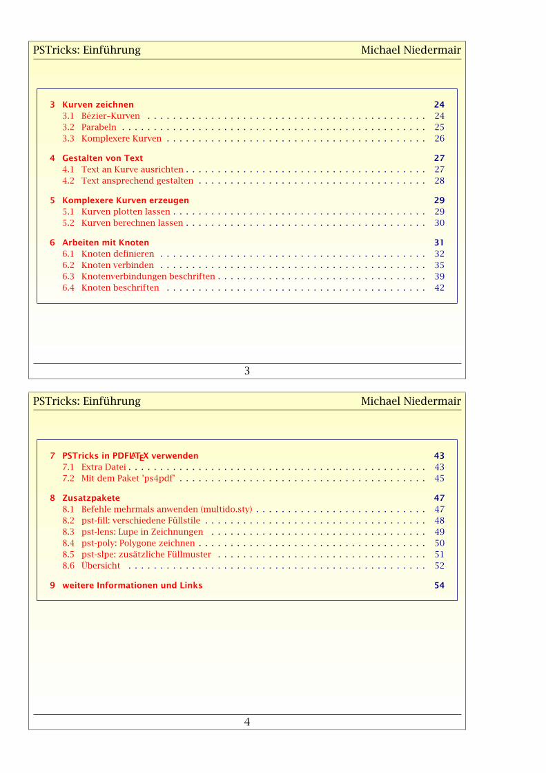
Inhalt
1 Grundlagen 51.1 PSTricks-Pakete einbinden . . . . . . . . . . . . . . . . . . . . . . . . . . . . . . . . . . . . . 5
1.2 Erstellen einer PSTricks-Umgebung (Koordinatensystem) . . . . . . . . . . . . . . . . . . 6
1.3 verwendete Einheiten . . . . . . . . . . . . . . . . . . . . . . . . . . . . . . . . . . . . . . . . 7
1.4 Linien zeichnen . . . . . . . . . . . . . . . . . . . . . . . . . . . . . . . . . . . . . . . . . . . . 9
1.5 andere Koordinatensysteme verwenden . . . . . . . . . . . . . . . . . . . . . . . . . . . . 12
2 Weitere Zeichenmöglichkeiten 152.1 Polygone . . . . . . . . . . . . . . . . . . . . . . . . . . . . . . . . . . . . . . . . . . . . . . . . 15
2.2 Rechtecke . . . . . . . . . . . . . . . . . . . . . . . . . . . . . . . . . . . . . . . . . . . . . . . 16
2.3 Rauten . . . . . . . . . . . . . . . . . . . . . . . . . . . . . . . . . . . . . . . . . . . . . . . . . 17
2.4 Dreicke . . . . . . . . . . . . . . . . . . . . . . . . . . . . . . . . . . . . . . . . . . . . . . . . . 18
2.5 Linienendungen . . . . . . . . . . . . . . . . . . . . . . . . . . . . . . . . . . . . . . . . . . . 19
2.6 Füllstile . . . . . . . . . . . . . . . . . . . . . . . . . . . . . . . . . . . . . . . . . . . . . . . . 21
2.7 Kreise . . . . . . . . . . . . . . . . . . . . . . . . . . . . . . . . . . . . . . . . . . . . . . . . . . 22
2.8 Kreiseausschnitte . . . . . . . . . . . . . . . . . . . . . . . . . . . . . . . . . . . . . . . . . . 23
PSTricks: Einführung Michael Niedermair
3
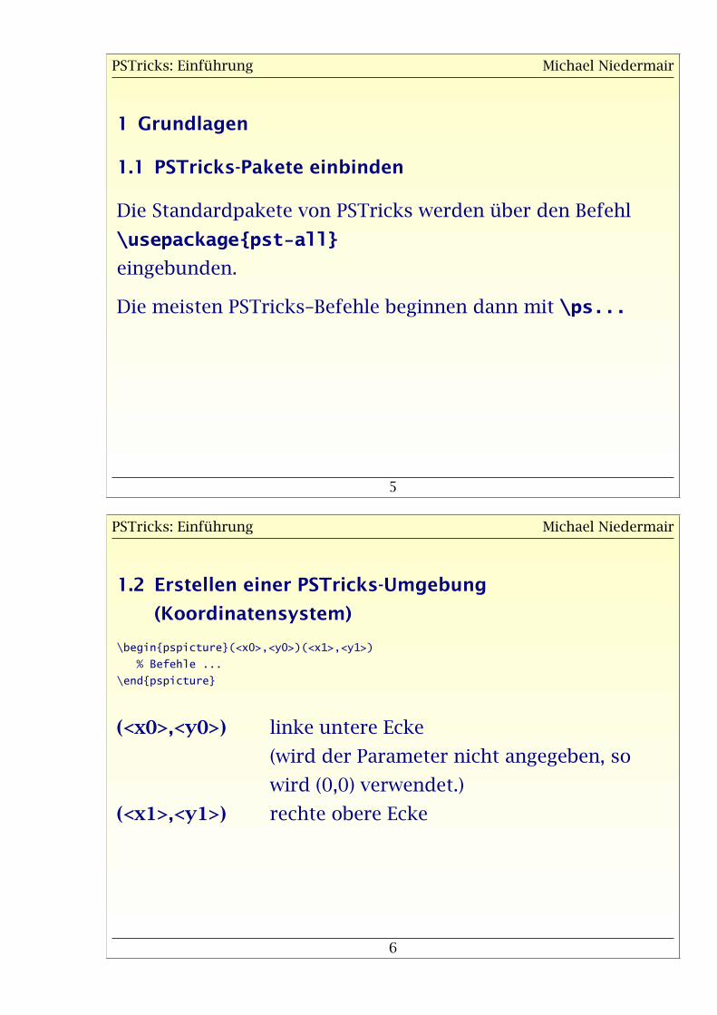
3 Kurven zeichnen 243.1 Bézier–Kurven . . . . . . . . . . . . . . . . . . . . . . . . . . . . . . . . . . . . . . . . . . . . 24
3.2 Parabeln . . . . . . . . . . . . . . . . . . . . . . . . . . . . . . . . . . . . . . . . . . . . . . . . 25
3.3 Komplexere Kurven . . . . . . . . . . . . . . . . . . . . . . . . . . . . . . . . . . . . . . . . . 26
4 Gestalten von Text 274.1 Text an Kurve ausrichten . . . . . . . . . . . . . . . . . . . . . . . . . . . . . . . . . . . . . . 27
4.2 Text ansprechend gestalten . . . . . . . . . . . . . . . . . . . . . . . . . . . . . . . . . . . . 28
5 Komplexere Kurven erzeugen 295.1 Kurven plotten lassen . . . . . . . . . . . . . . . . . . . . . . . . . . . . . . . . . . . . . . . . 29
5.2 Kurven berechnen lassen . . . . . . . . . . . . . . . . . . . . . . . . . . . . . . . . . . . . . . 30
6 Arbeiten mit Knoten 316.1 Knoten definieren . . . . . . . . . . . . . . . . . . . . . . . . . . . . . . . . . . . . . . . . . . 32
6.2 Knoten verbinden . . . . . . . . . . . . . . . . . . . . . . . . . . . . . . . . . . . . . . . . . . 35
6.3 Knotenverbindungen beschriften . . . . . . . . . . . . . . . . . . . . . . . . . . . . . . . . . 39
6.4 Knoten beschriften . . . . . . . . . . . . . . . . . . . . . . . . . . . . . . . . . . . . . . . . . 42
PSTricks: Einführung Michael Niedermair
4
7 PSTricks in PDFLATEX verwenden 437.1 Extra Datei . . . . . . . . . . . . . . . . . . . . . . . . . . . . . . . . . . . . . . . . . . . . . . . 43
7.2 Mit dem Paket ’ps4pdf’ . . . . . . . . . . . . . . . . . . . . . . . . . . . . . . . . . . . . . . . 45
8 Zusatzpakete 478.1 Befehle mehrmals anwenden (multido.sty) . . . . . . . . . . . . . . . . . . . . . . . . . . . 47
8.2 pst-fill: verschiedene Füllstile . . . . . . . . . . . . . . . . . . . . . . . . . . . . . . . . . . . 48
8.3 pst-lens: Lupe in Zeichnungen . . . . . . . . . . . . . . . . . . . . . . . . . . . . . . . . . . 49
8.4 pst-poly: Polygone zeichnen . . . . . . . . . . . . . . . . . . . . . . . . . . . . . . . . . . . . 50
8.5 pst-slpe: zusätzliche Füllmuster . . . . . . . . . . . . . . . . . . . . . . . . . . . . . . . . . 51
8.6 Übersicht . . . . . . . . . . . . . . . . . . . . . . . . . . . . . . . . . . . . . . . . . . . . . . . 52
9 weitere Informationen und Links 54
PSTricks: Einführung Michael Niedermair
5
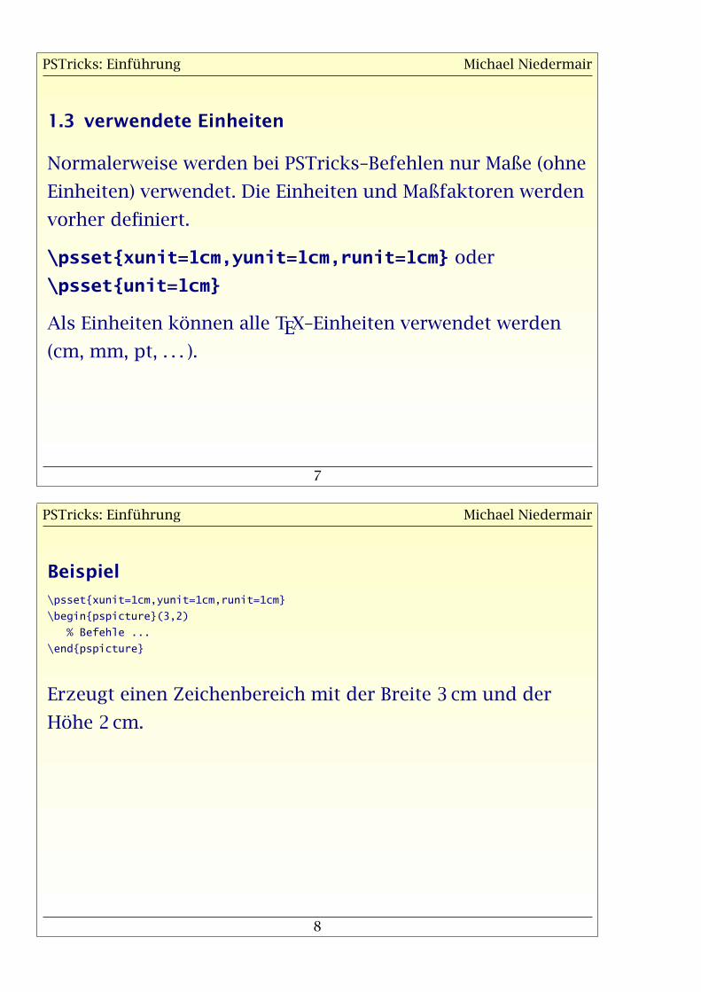
1 Grundlagen
1.1 PSTricks-Pakete einbinden
Die Standardpakete von PSTricks werden über den Befehl
\usepackage{pst-all}
eingebunden.
Die meisten PSTricks–Befehle beginnen dann mit \ps...
PSTricks: Einführung Michael Niedermair
6
1.2 Erstellen einer PSTricks-Umgebung
(Koordinatensystem)
\begin{pspicture}(<x0>,<y0>)(<x1>,<y1>)
% Befehle ...
\end{pspicture}
(<x0>,<y0>) linke untere Ecke
(wird der Parameter nicht angegeben, so
wird (0,0) verwendet.)
(<x1>,<y1>) rechte obere Ecke
PSTricks: Einführung Michael Niedermair
7
1.3 verwendete Einheiten
Normalerweise werden bei PSTricks–Befehlen nur Maße (ohne
Einheiten) verwendet. Die Einheiten und Maßfaktoren werden
vorher definiert.
\psset{xunit=1cm,yunit=1cm,runit=1cm} oder
\psset{unit=1cm}
Als Einheiten können alle TEX–Einheiten verwendet werden
(cm, mm, pt, . . . ).
PSTricks: Einführung Michael Niedermair
8
Beispiel
\psset{xunit=1cm,yunit=1cm,runit=1cm}
\begin{pspicture}(3,2)
% Befehle ...
\end{pspicture}
Erzeugt einen Zeichenbereich mit der Breite 3 cm und der
Höhe 2 cm.
PSTricks: Einführung Michael Niedermair
9
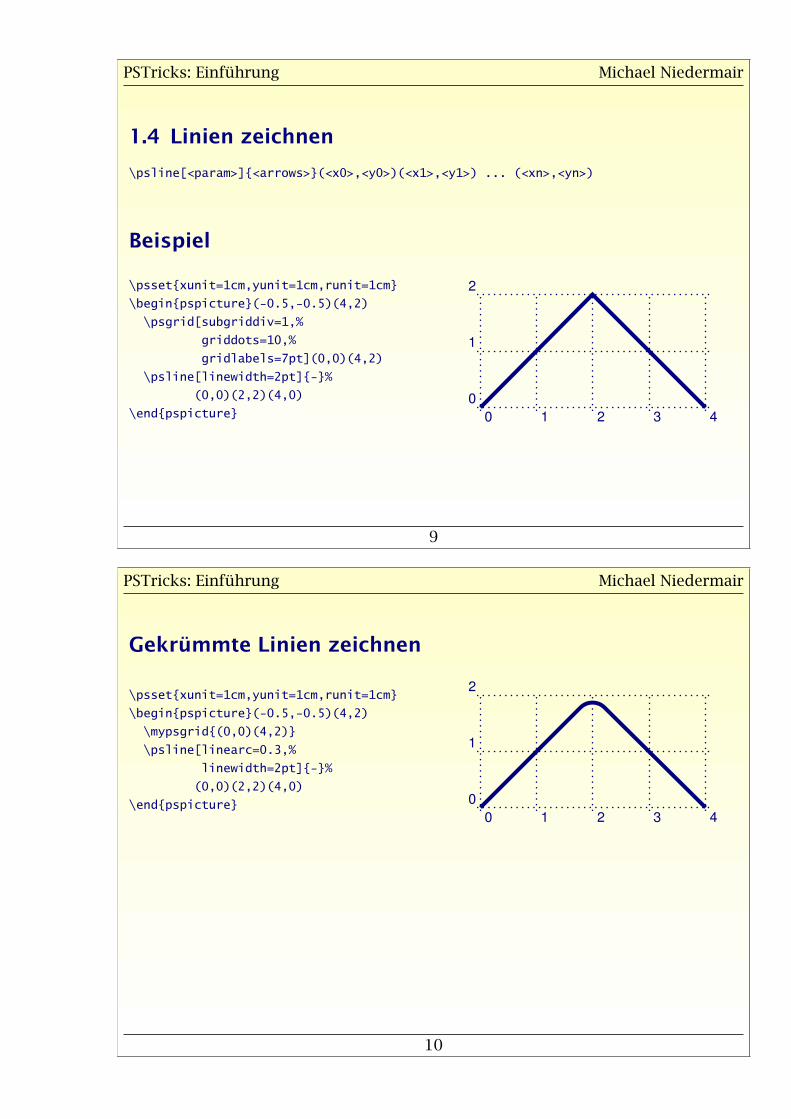
1.4 Linien zeichnen
\psline[<param>]{<arrows>}(<x0>,<y0>)(<x1>,<y1>) ... (<xn>,<yn>)
Beispiel
\psset{xunit=1cm,yunit=1cm,runit=1cm}
\begin{pspicture}(-0.5,-0.5)(4,2)
\psgrid[subgriddiv=1,%
griddots=10,%
gridlabels=7pt](0,0)(4,2)
\psline[linewidth=2pt]{-}%
(0,0)(2,2)(4,0)
\end{pspicture} 0 1 2 3 4
0
1
2
PSTricks: Einführung Michael Niedermair
10
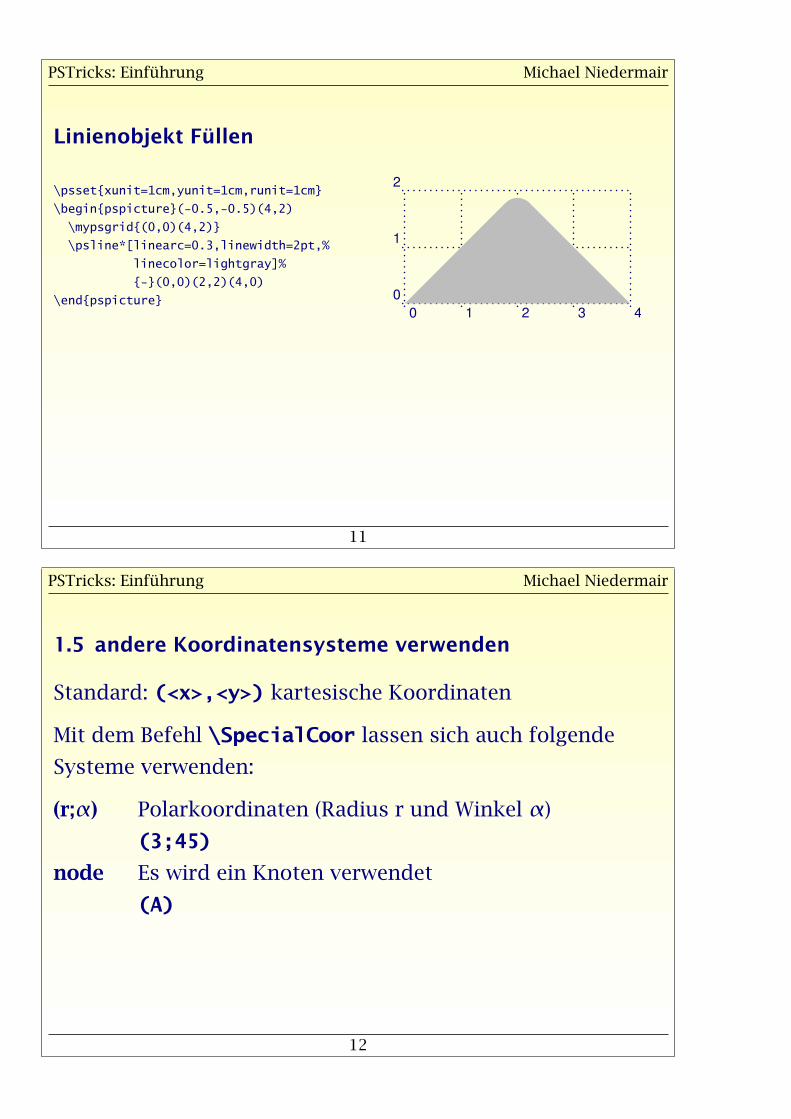
Gekrümmte Linien zeichnen
\psset{xunit=1cm,yunit=1cm,runit=1cm}
\begin{pspicture}(-0.5,-0.5)(4,2)
\mypsgrid{(0,0)(4,2)}
\psline[linearc=0.3,%
linewidth=2pt]{-}%
(0,0)(2,2)(4,0)
\end{pspicture}0 1 2 3 4
0
1
2
PSTricks: Einführung Michael Niedermair
11
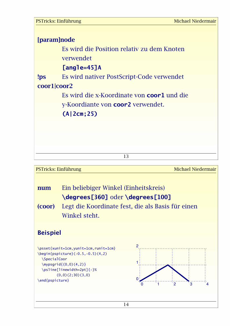
Linienobjekt Füllen
\psset{xunit=1cm,yunit=1cm,runit=1cm}
\begin{pspicture}(-0.5,-0.5)(4,2)
\mypsgrid{(0,0)(4,2)}
\psline*[linearc=0.3,linewidth=2pt,%
linecolor=lightgray]%
{-}(0,0)(2,2)(4,0)
\end{pspicture}0 1 2 3 4
0
1
2
PSTricks: Einführung Michael Niedermair
12
1.5 andere Koordinatensysteme verwenden
Standard: (<x>,<y>) kartesische Koordinaten
Mit dem Befehl \SpecialCoor lassen sich auch folgende
Systeme verwenden:
(r;α) Polarkoordinaten (Radius r und Winkel α)
(3;45)
node Es wird ein Knoten verwendet
(A)
PSTricks: Einführung Michael Niedermair
13
[param]node
Es wird die Position relativ zu dem Knoten
verwendet
[angle=45]A
!ps Es wird nativer PostScript-Code verwendet
coor1|coor2
Es wird die x-Koordinate von coor1 und die
y-Koordiante von coor2 verwendet.
(A|2cm;25)
PSTricks: Einführung Michael Niedermair
14
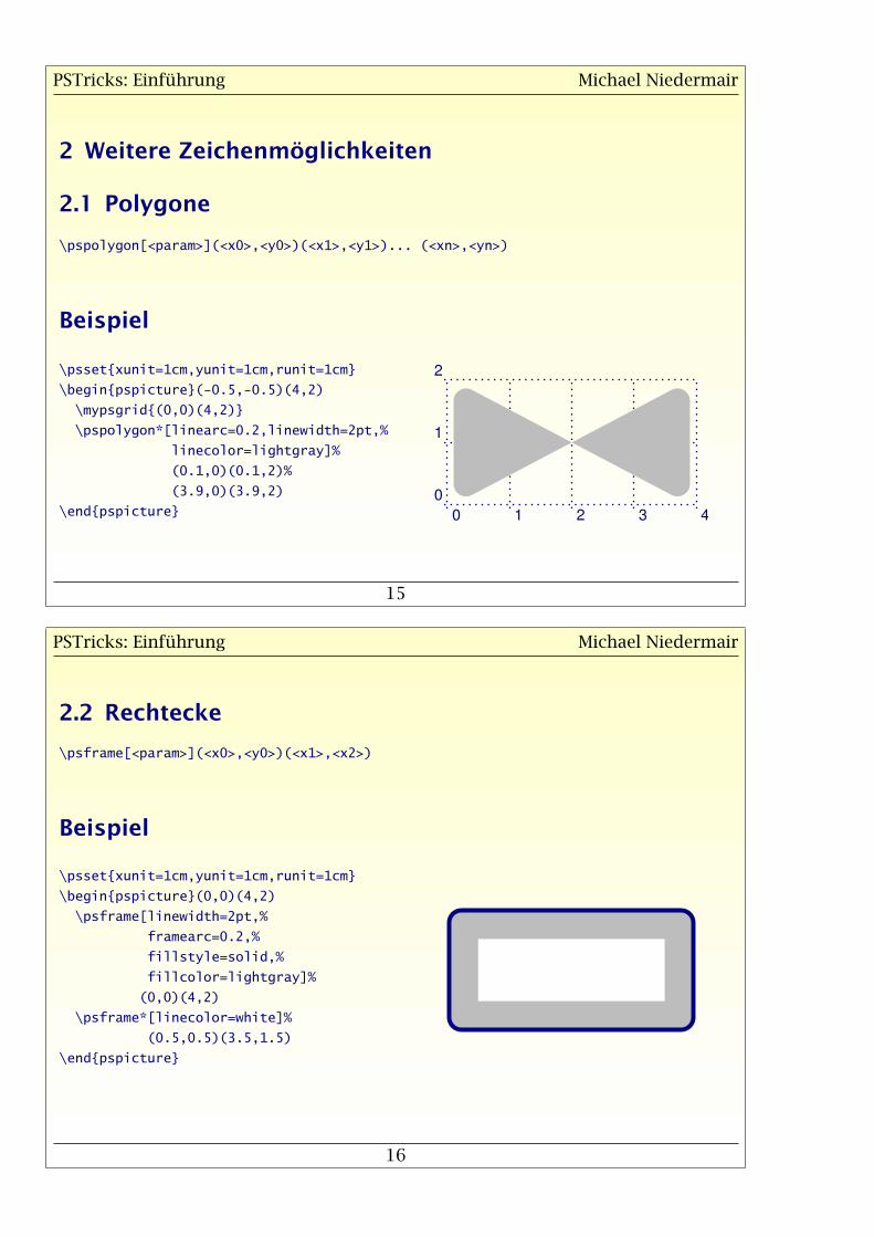
num Ein beliebiger Winkel (Einheitskreis)
\degrees[360] oder \degrees[100]
(coor) Legt die Koordinate fest, die als Basis für einen
Winkel steht.
Beispiel
\psset{xunit=1cm,yunit=1cm,runit=1cm}
\begin{pspicture}(-0.5,-0.5)(4,2)
\SpecialCoor
\mypsgrid{(0,0)(4,2)}
\psline[linewidth=2pt]{-}%
(0,0)(2;30)(3,0)
\end{pspicture}0 1 2 3 4
0
1
2
PSTricks: Einführung Michael Niedermair
15
2 Weitere Zeichenmöglichkeiten
2.1 Polygone
\pspolygon[<param>](<x0>,<y0>)(<x1>,<y1>)... (<xn>,<yn>)
Beispiel
\psset{xunit=1cm,yunit=1cm,runit=1cm}
\begin{pspicture}(-0.5,-0.5)(4,2)
\mypsgrid{(0,0)(4,2)}
\pspolygon*[linearc=0.2,linewidth=2pt,%
linecolor=lightgray]%
(0.1,0)(0.1,2)%
(3.9,0)(3.9,2)
\end{pspicture} 0 1 2 3 4
0
1
2
PSTricks: Einführung Michael Niedermair
16
2.2 Rechtecke
\psframe[<param>](<x0>,<y0>)(<x1>,<x2>)
Beispiel
\psset{xunit=1cm,yunit=1cm,runit=1cm}
\begin{pspicture}(0,0)(4,2)
\psframe[linewidth=2pt,%
framearc=0.2,%
fillstyle=solid,%
fillcolor=lightgray]%
(0,0)(4,2)
\psframe*[linecolor=white]%
(0.5,0.5)(3.5,1.5)
\end{pspicture}
PSTricks: Einführung Michael Niedermair
17
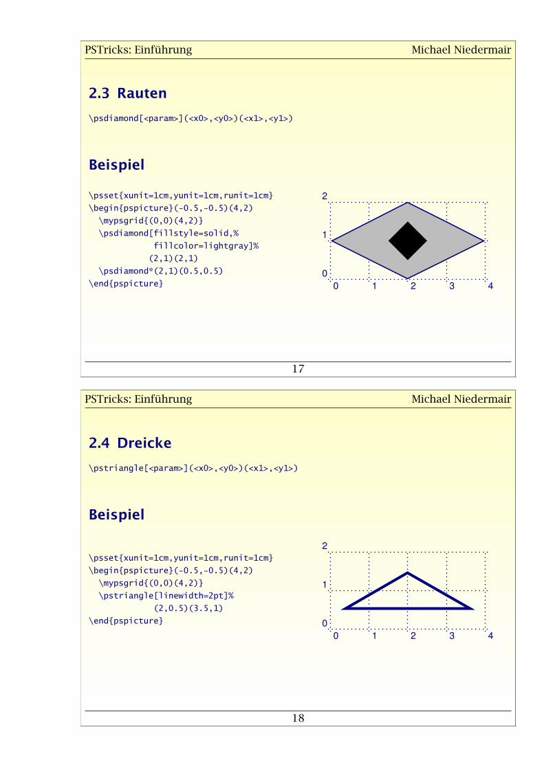
2.3 Rauten
\psdiamond[<param>](<x0>,<y0>)(<x1>,<y1>)
Beispiel
\psset{xunit=1cm,yunit=1cm,runit=1cm}
\begin{pspicture}(-0.5,-0.5)(4,2)
\mypsgrid{(0,0)(4,2)}
\psdiamond[fillstyle=solid,%
fillcolor=lightgray]%
(2,1)(2,1)
\psdiamond*(2,1)(0.5,0.5)
\end{pspicture} 0 1 2 3 4
0
1
2
PSTricks: Einführung Michael Niedermair
18
2.4 Dreicke
\pstriangle[<param>](<x0>,<y0>)(<x1>,<y1>)
Beispiel
\psset{xunit=1cm,yunit=1cm,runit=1cm}
\begin{pspicture}(-0.5,-0.5)(4,2)
\mypsgrid{(0,0)(4,2)}
\pstriangle[linewidth=2pt]%
(2,0.5)(3.5,1)
\end{pspicture}
0 1 2 3 4
0
1
2
PSTricks: Einführung Michael Niedermair
19
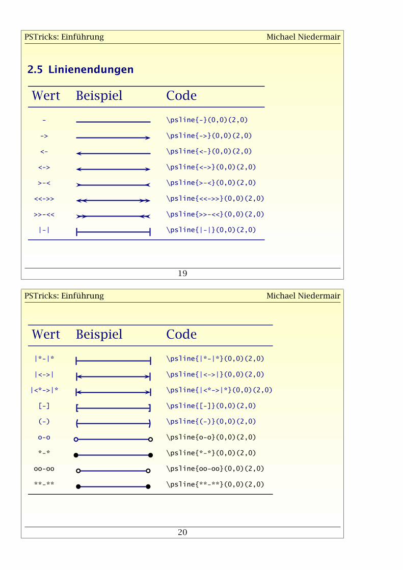
2.5 Linienendungen
Wert Beispiel Code
\psline{}(0,0)(2,0)
> \psline{>}(0,0)(2,0)
< \psline{<}(0,0)(2,0)
<> \psline{<>}(0,0)(2,0)
>< \psline{><}(0,0)(2,0)
<<>> \psline{<<>>}(0,0)(2,0)
>><< \psline{>><<}(0,0)(2,0)
|| \psline{||}(0,0)(2,0)
PSTricks: Einführung Michael Niedermair
20
Wert Beispiel Code
|*|* \psline{|*|*}(0,0)(2,0)
|<>| \psline{|<>|}(0,0)(2,0)
|<*>|* \psline{|<*>|*}(0,0)(2,0)
[] \psline{[]}(0,0)(2,0)
() \psline{()}(0,0)(2,0)
oo \psline{oo}(0,0)(2,0)
** \psline{**}(0,0)(2,0)
oooo \psline{oooo}(0,0)(2,0)
**** \psline{****}(0,0)(2,0)
PSTricks: Einführung Michael Niedermair
21
2.6 Füllstile
\psset{xunit=1cm,yunit=1cm,runit=1cm}
\begin{pspicture}(0,0)(4,3)
\psframe[linestyle=none,%
fillstyle=gradient,%
gradangle=90,%
gradbegin=lightgray,%
gradend=white,%
gradmidpoint=1]%
(0,0)(2,3)
\psframe[linestyle=none,%
fillstyle=gradient,%
gradangle=90,%
gradbegin=white,%
gradend=black,%
gradmidpoint=1]%
(2,0)(4,3)
\psframe[linewidth=2pt](0,0)(4,3)
\end{pspicture}
PSTricks: Einführung Michael Niedermair
22
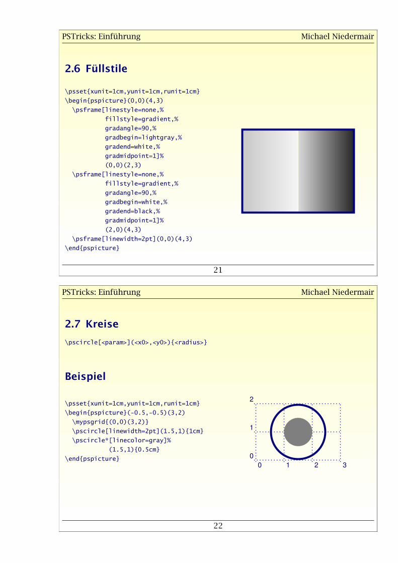
2.7 Kreise
\pscircle[<param>](<x0>,<y0>){<radius>}
Beispiel
\psset{xunit=1cm,yunit=1cm,runit=1cm}
\begin{pspicture}(-0.5,-0.5)(3,2)
\mypsgrid{(0,0)(3,2)}
\pscircle[linewidth=2pt](1.5,1){1cm}
\pscircle*[linecolor=gray]%
(1.5,1){0.5cm}
\end{pspicture}0 1 2 3
0
1
2
PSTricks: Einführung Michael Niedermair
23
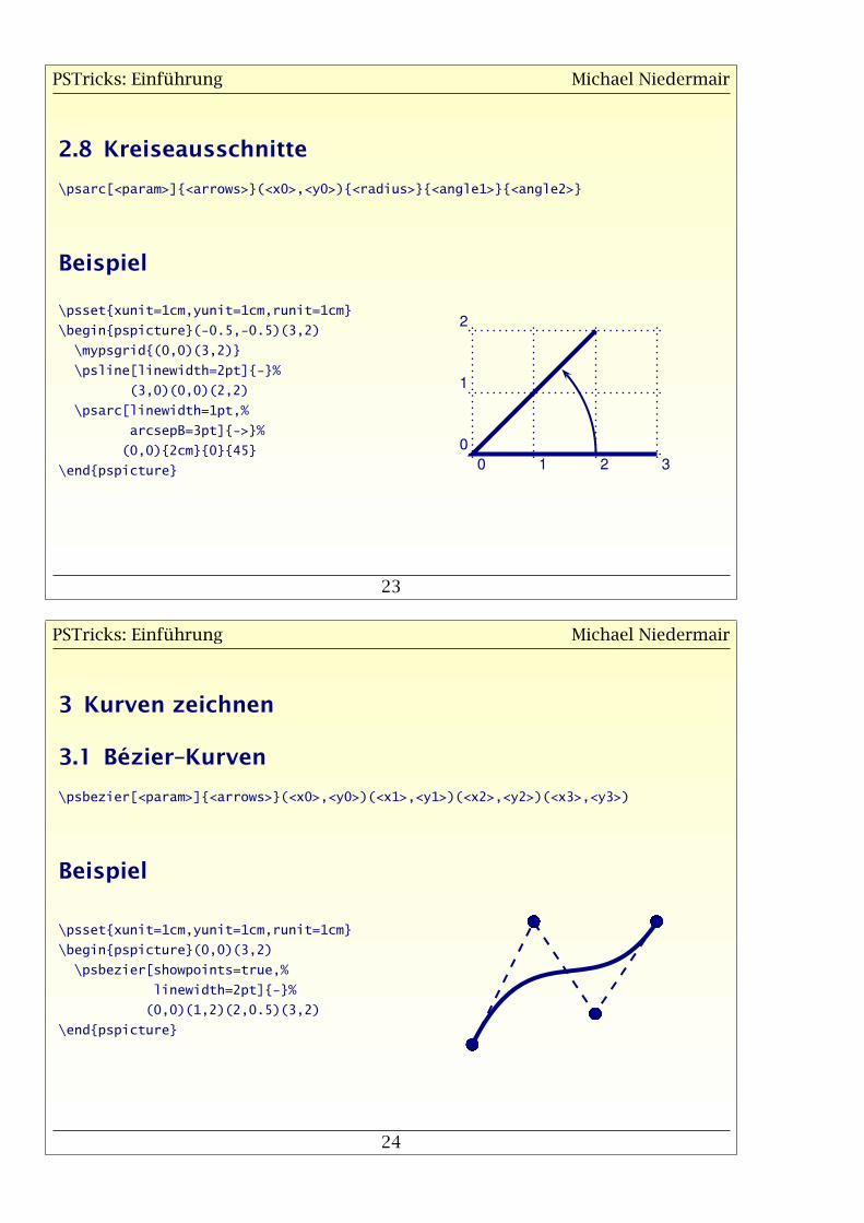
2.8 Kreiseausschnitte
\psarc[<param>]{<arrows>}(<x0>,<y0>){<radius>}{<angle1>}{<angle2>}
Beispiel
\psset{xunit=1cm,yunit=1cm,runit=1cm}
\begin{pspicture}(-0.5,-0.5)(3,2)
\mypsgrid{(0,0)(3,2)}
\psline[linewidth=2pt]{-}%
(3,0)(0,0)(2,2)
\psarc[linewidth=1pt,%
arcsepB=3pt]{->}%
(0,0){2cm}{0}{45}
\end{pspicture} 0 1 2 3
0
1
2
PSTricks: Einführung Michael Niedermair
24
3 Kurven zeichnen
3.1 Bézier–Kurven
\psbezier[<param>]{<arrows>}(<x0>,<y0>)(<x1>,<y1>)(<x2>,<y2>)(<x3>,<y3>)
Beispiel
\psset{xunit=1cm,yunit=1cm,runit=1cm}
\begin{pspicture}(0,0)(3,2)
\psbezier[showpoints=true,%
linewidth=2pt]{-}%
(0,0)(1,2)(2,0.5)(3,2)
\end{pspicture} �
�
�
�
PSTricks: Einführung Michael Niedermair
25
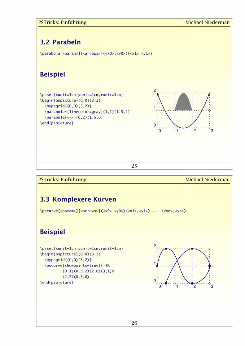
3.2 Parabeln
\parabola[<param>]{<arrows>}(<x0>,<y0>)(<x1>,<y1>)
Beispiel
\psset{xunit=1cm,yunit=1cm,runit=1cm}
\begin{pspicture}(0,0)(3,2)
\mypsgrid{(0,0)(3,2)}
\parabola*[linecolor=gray](1,1)(1.5,2)
\parabola{<->}(0,2)(1.5,0)
\end{pspicture}
0 1 2 3
0
1
2
PSTricks: Einführung Michael Niedermair
26
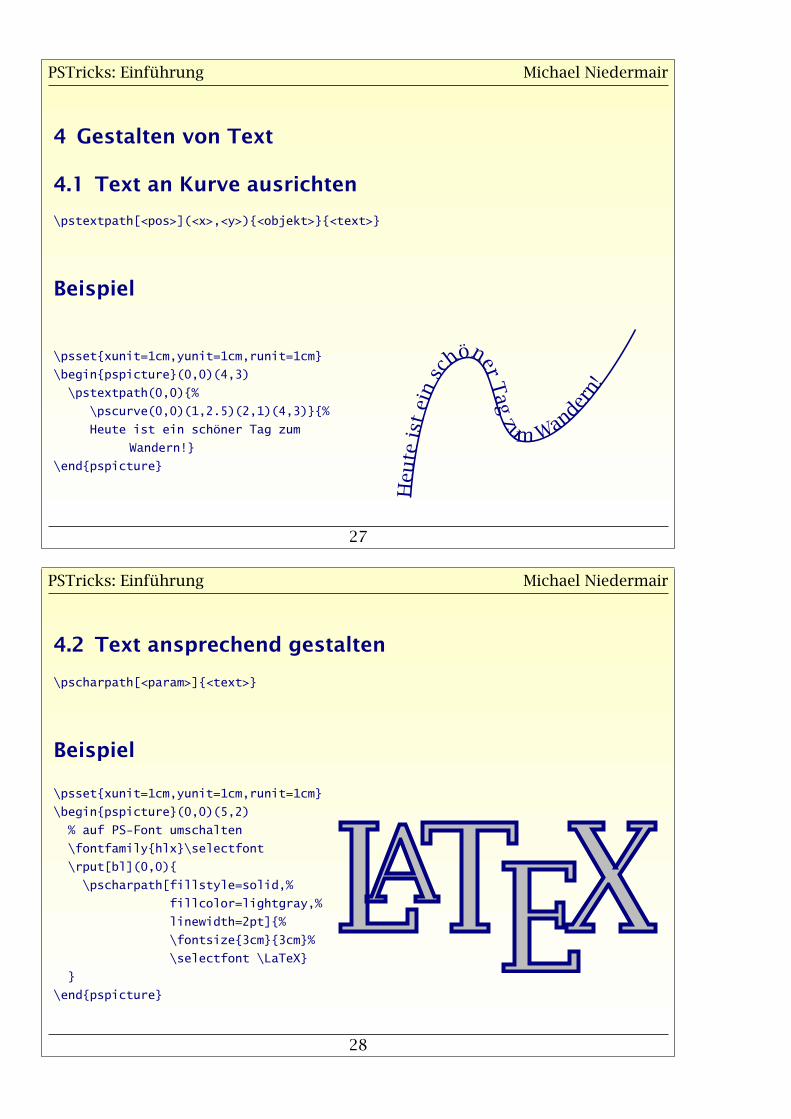
3.3 Komplexere Kurven
\pscurve[<param>]{<arrows>}(<x0>,<y0>)(<x1>,<y1>) ... (<xn>,<yn>)
Beispiel
\psset{xunit=1cm,yunit=1cm,runit=1cm}
\begin{pspicture}(0,0)(3,2)
\mypsgrid{(0,0)(3,2)}
\pscurve[showpoints=true]{-}%
(0,1)(0.5,2)(2,0)(3,1)%
(2,2)(0.5,0)
\end{pspicture}0 1 2 3
0
1
2
�
�
�
�
�
�
PSTricks: Einführung Michael Niedermair
27
4 Gestalten von Text
4.1 Text an Kurve ausrichten
\pstextpath[<pos>](<x>,<y>){<objekt>}{<text>}
Beispiel
\psset{xunit=1cm,yunit=1cm,runit=1cm}
\begin{pspicture}(0,0)(4,3)
\pstextpath(0,0){%
\pscurve(0,0)(1,2.5)(2,1)(4,3)}{%
Heute ist ein schöner Tag zum
Wandern!}
\end{pspicture}
Heu
teis
tein
sc
hönerT
ag
z
um Wan
dern
!PSTricks: Einführung Michael Niedermair
28
4.2 Text ansprechend gestalten
\pscharpath[<param>]{<text>}
Beispiel
\psset{xunit=1cm,yunit=1cm,runit=1cm}
\begin{pspicture}(0,0)(5,2)
% auf PS-Font umschalten
\fontfamily{hlx}\selectfont
\rput[bl](0,0){
\pscharpath[fillstyle=solid,%
fillcolor=lightgray,%
linewidth=2pt]{%
\fontsize{3cm}{3cm}%
\selectfont \LaTeX}
}
\end{pspicture}
PSTricks: Einführung Michael Niedermair
29
5 Komplexere Kurven erzeugen
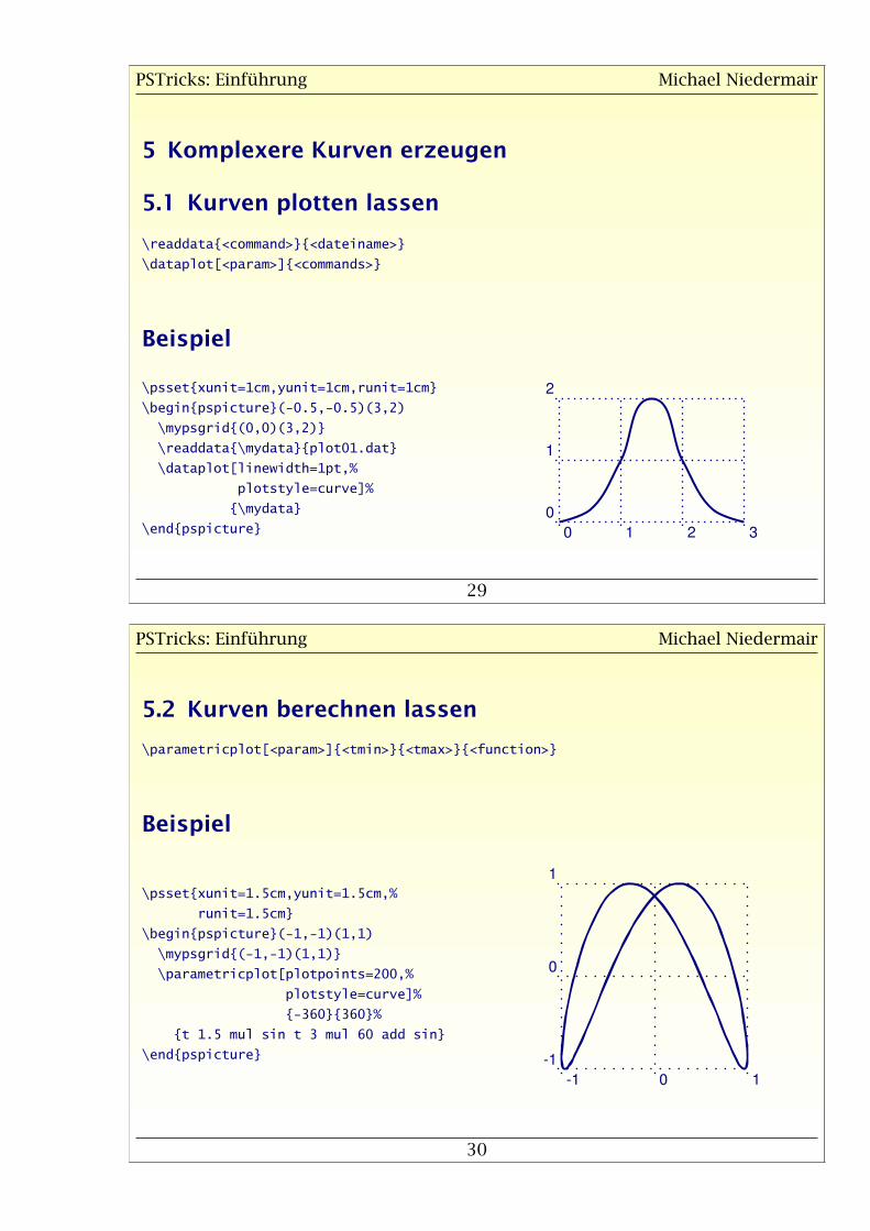
5.1 Kurven plotten lassen
\readdata{<command>}{<dateiname>}
\dataplot[<param>]{<commands>}
Beispiel
\psset{xunit=1cm,yunit=1cm,runit=1cm}
\begin{pspicture}(-0.5,-0.5)(3,2)
\mypsgrid{(0,0)(3,2)}
\readdata{\mydata}{plot01.dat}
\dataplot[linewidth=1pt,%
plotstyle=curve]%
{\mydata}
\end{pspicture} 0 1 2 3
0
1
2
PSTricks: Einführung Michael Niedermair
30
5.2 Kurven berechnen lassen
\parametricplot[<param>]{<tmin>}{<tmax>}{<function>}
Beispiel
\psset{xunit=1.5cm,yunit=1.5cm,%
runit=1.5cm}
\begin{pspicture}(-1,-1)(1,1)
\mypsgrid{(-1,-1)(1,1)}
\parametricplot[plotpoints=200,%
plotstyle=curve]%
{-360}{360}%
{t 1.5 mul sin t 3 mul 60 add sin}
\end{pspicture}
-1 0 1
-1
0
1
PSTricks: Einführung Michael Niedermair
31
6 Arbeiten mit Knoten
Knoten stellen Punkte im KO-System dar, welche beliebig für
• Objekte,
• Verbindungslinien,
• Beschriftungen,
• etc.
verwendet werden können.
PSTricks: Einführung Michael Niedermair
32
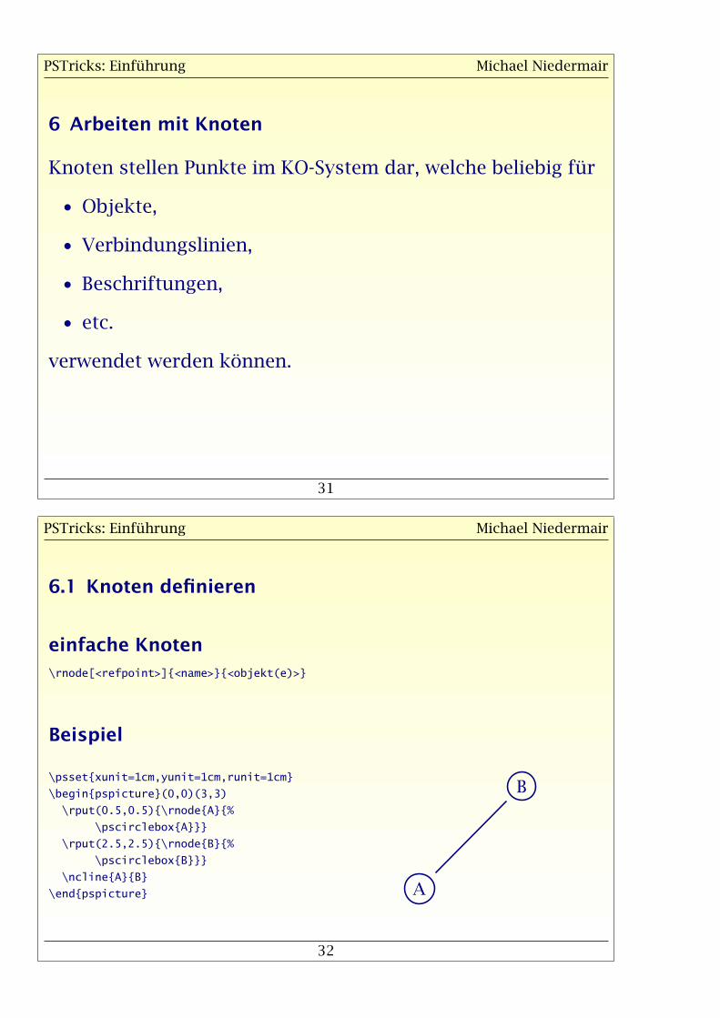
6.1 Knoten definieren
einfache Knoten
\rnode[<refpoint>]{<name>}{<objekt(e)>}
Beispiel
\psset{xunit=1cm,yunit=1cm,runit=1cm}
\begin{pspicture}(0,0)(3,3)
\rput(0.5,0.5){\rnode{A}{%
\pscirclebox{A}}}
\rput(2.5,2.5){\rnode{B}{%
\pscirclebox{B}}}
\ncline{A}{B}
\end{pspicture} A
B
PSTricks: Einführung Michael Niedermair
33
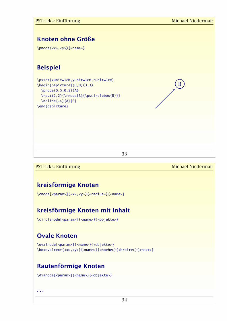
Knoten ohne Größe
\pnode(<x>,<y>){<name>}
Beispiel
\psset{xunit=1cm,yunit=1cm,runit=1cm}
\begin{pspicture}(0,0)(3,3)
\pnode(0.5,0.5){A}
\rput(2,2){\rnode{B}{\pscirclebox{B}}}
\ncline{->}{A}{B}
\end{pspicture}
B
PSTricks: Einführung Michael Niedermair
34
kreisförmige Knoten
\cnode[<param>](<x>,<y>){<radius>}{<name>}
kreisförmige Knoten mit Inhalt
\circlenode[<param>]{<name>}{<objekte>}
Ovale Knoten\ovalnode[<param>]{<name>}{<objekte>}
\boxovaltext{<x>,<y>}{<name>}{<hoehe>}{<breite>}{<text>}
Rautenförmige Knoten
\dianode[<param>]{<name>}{<objekte>}
. . .
PSTricks: Einführung Michael Niedermair
35
6.2 Knoten verbinden
Linie
\ncline[<param>]{<arrows>}{<nodeA>}{<nodeB>}
Beispiel
\psset{xunit=1cm,yunit=1cm,runit=1cm}
\begin{pspicture}(0,0)(3,2.5)
\rput[bl](0.5,0.5){\rnode{A}{Text1}}
\rput[tr](2.5,2.5){\rnode{B}{Text2}}
\psset{nodesep=4pt,offset=4pt,%
arrows=->}
\ncline{A}{B}
\ncline{B}{A}
\end{pspicture}
Text1
Text2
PSTricks: Einführung Michael Niedermair
36
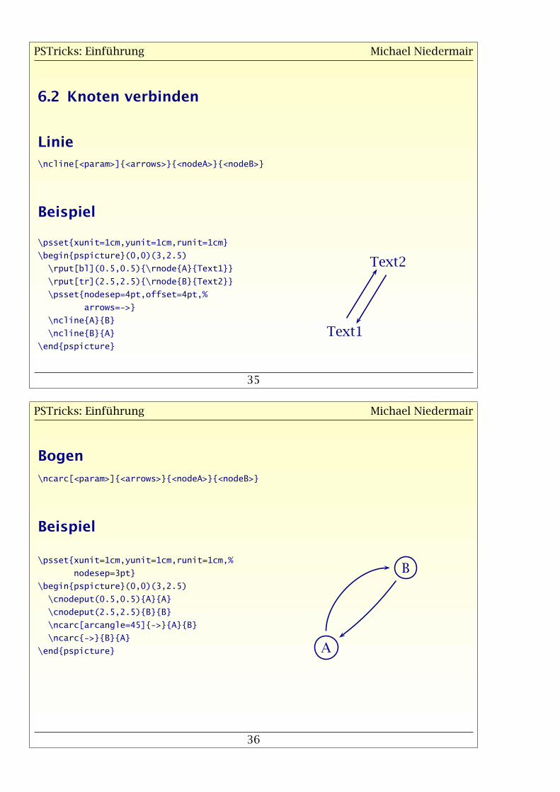
Bogen
\ncarc[<param>]{<arrows>}{<nodeA>}{<nodeB>}
Beispiel
\psset{xunit=1cm,yunit=1cm,runit=1cm,%
nodesep=3pt}
\begin{pspicture}(0,0)(3,2.5)
\cnodeput(0.5,0.5){A}{A}
\cnodeput(2.5,2.5){B}{B}
\ncarc[arcangle=45]{->}{A}{B}
\ncarc{->}{B}{A}
\end{pspicture} A
B
PSTricks: Einführung Michael Niedermair
37
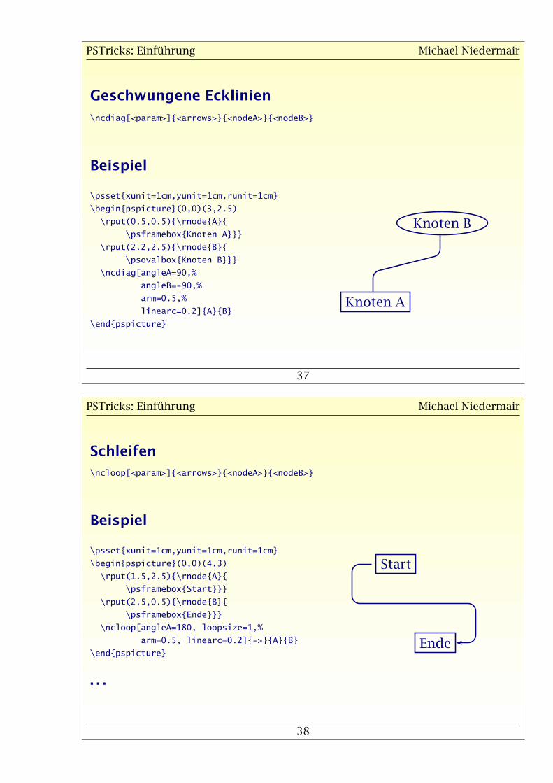
Geschwungene Ecklinien
\ncdiag[<param>]{<arrows>}{<nodeA>}{<nodeB>}
Beispiel
\psset{xunit=1cm,yunit=1cm,runit=1cm}
\begin{pspicture}(0,0)(3,2.5)
\rput(0.5,0.5){\rnode{A}{
\psframebox{Knoten A}}}
\rput(2.2,2.5){\rnode{B}{
\psovalbox{Knoten B}}}
\ncdiag[angleA=90,%
angleB=-90,%
arm=0.5,%
linearc=0.2]{A}{B}
\end{pspicture}
Knoten A
Knoten B
PSTricks: Einführung Michael Niedermair
38
Schleifen
\ncloop[<param>]{<arrows>}{<nodeA>}{<nodeB>}
Beispiel
\psset{xunit=1cm,yunit=1cm,runit=1cm}
\begin{pspicture}(0,0)(4,3)
\rput(1.5,2.5){\rnode{A}{
\psframebox{Start}}}
\rput(2.5,0.5){\rnode{B}{
\psframebox{Ende}}}
\ncloop[angleA=180, loopsize=1,%
arm=0.5, linearc=0.2]{->}{A}{B}
\end{pspicture}
Start
Ende
. . .
PSTricks: Einführung Michael Niedermair
39
6.3 Knotenverbindungen beschriften
horizontal\ncput[<param>]{<objekte>}
\naput[<param>]{<objekte>}
\nbput[<param>{<objekte>}
\psset{xunit=1cm,yunit=1cm,runit=1cm,%
nodesep=3pt,linewidth=1pt}
\begin{pspicture}(0,-1)(4,4)
\cnode(0.5,1.5){0.4cm}{M}
\cnode*(3.5,3){5pt}{A}
\cnode*(3.5,1.5){5pt}{B}
\cnode*(3.5,0){5pt}{C}
\ncline{M}{A}\naput{über}
\ncline{M}{B}\ncput*{auf}
\ncline{M}{C}\nbput{unter}
\end{pspicture}
über
auf
unter
PSTricks: Einführung Michael Niedermair
40
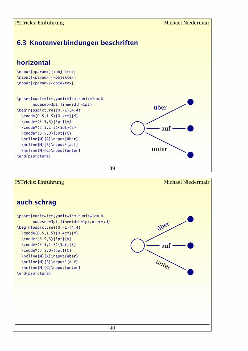
auch schräg
\psset{xunit=1cm,yunit=1cm,runit=1cm,%
nodesep=3pt,linewidth=1pt,nrot=:U}
\begin{pspicture}(0,-1)(4,4)
\cnode(0.5,1.5){0.4cm}{M}
\cnode*(3.5,3){5pt}{A}
\cnode*(3.5,1.5){5pt}{B}
\cnode*(3.5,0){5pt}{C}
\ncline{M}{A}\naput{über}
\ncline{M}{B}\ncput*{auf}
\ncline{M}{C}\nbput{unter}
\end{pspicture}
über
auf
unter
PSTricks: Einführung Michael Niedermair
41
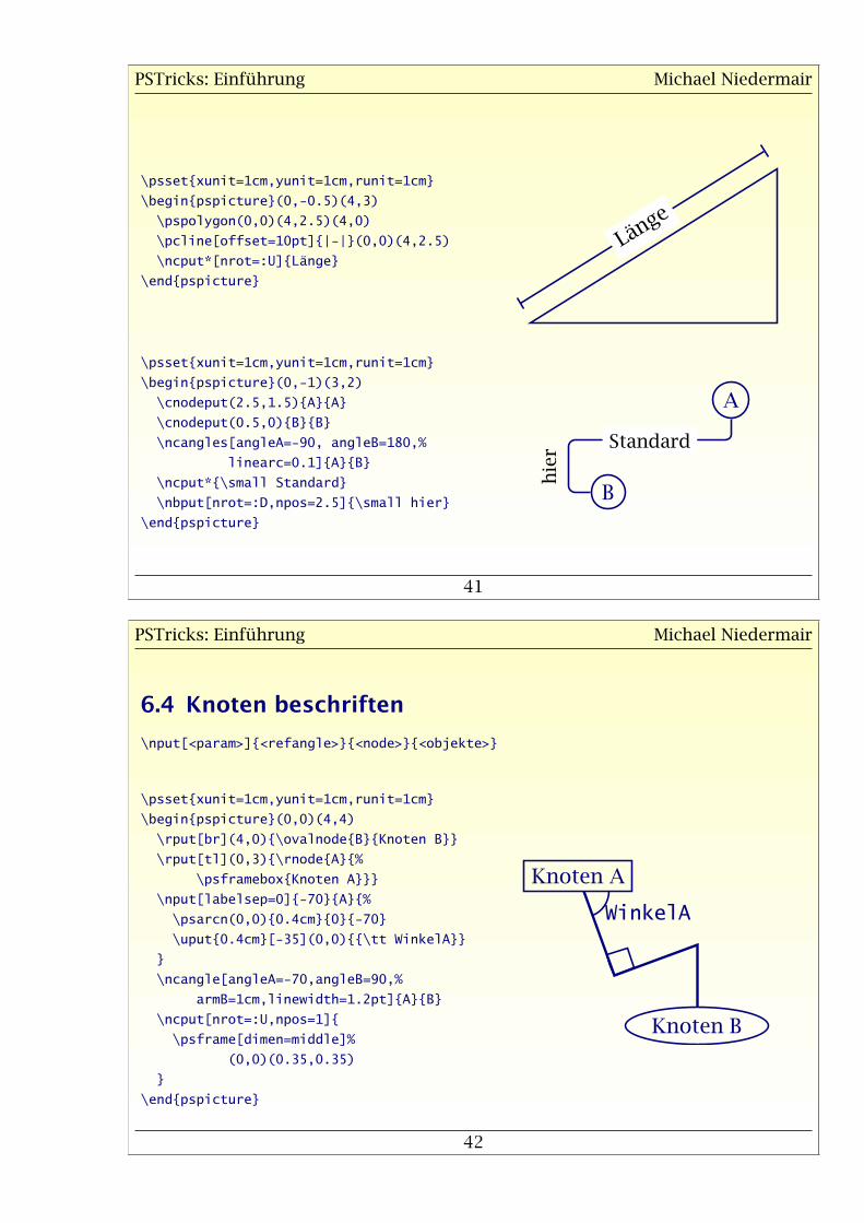
\psset{xunit=1cm,yunit=1cm,runit=1cm}
\begin{pspicture}(0,-0.5)(4,3)
\pspolygon(0,0)(4,2.5)(4,0)
\pcline[offset=10pt]{|-|}(0,0)(4,2.5)
\ncput*[nrot=:U]{Länge}
\end{pspicture}
Länge
\psset{xunit=1cm,yunit=1cm,runit=1cm}
\begin{pspicture}(0,-1)(3,2)
\cnodeput(2.5,1.5){A}{A}
\cnodeput(0.5,0){B}{B}
\ncangles[angleA=-90, angleB=180,%
linearc=0.1]{A}{B}
\ncput*{\small Standard}
\nbput[nrot=:D,npos=2.5]{\small hier}
\end{pspicture}
A
B
Standard
hie
r
PSTricks: Einführung Michael Niedermair
42
6.4 Knoten beschriften
\nput[<param>]{<refangle>}{<node>}{<objekte>}
\psset{xunit=1cm,yunit=1cm,runit=1cm}
\begin{pspicture}(0,0)(4,4)
\rput[br](4,0){\ovalnode{B}{Knoten B}}
\rput[tl](0,3){\rnode{A}{%
\psframebox{Knoten A}}}
\nput[labelsep=0]{-70}{A}{%
\psarcn(0,0){0.4cm}{0}{-70}
\uput{0.4cm}[-35](0,0){{\tt WinkelA}}
}
\ncangle[angleA=-70,angleB=90,%
armB=1cm,linewidth=1.2pt]{A}{B}
\ncput[nrot=:U,npos=1]{
\psframe[dimen=middle]%
(0,0)(0.35,0.35)
}
\end{pspicture}
Knoten B
Knoten A
WinkelA
PSTricks: Einführung Michael Niedermair
43
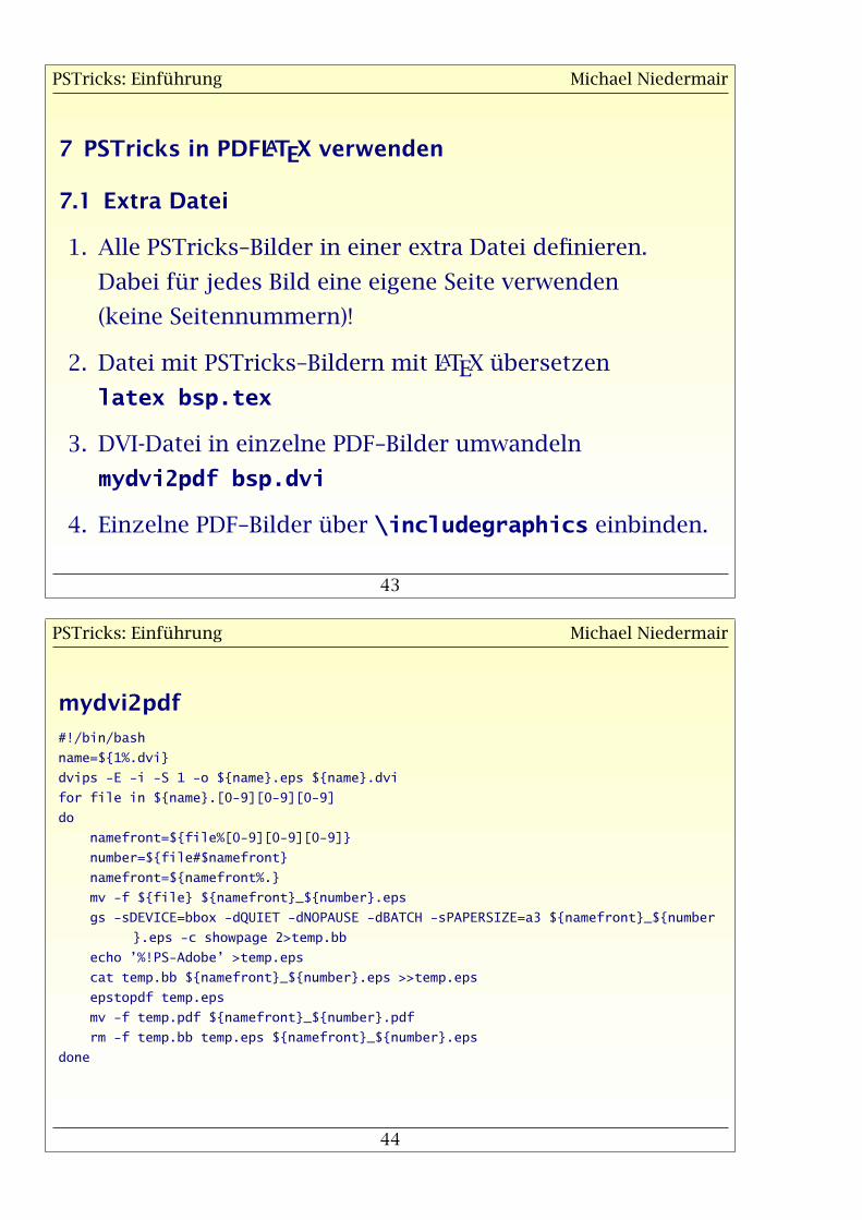
7 PSTricks in PDFLATEX verwenden
7.1 Extra Datei
1. Alle PSTricks–Bilder in einer extra Datei definieren.
Dabei für jedes Bild eine eigene Seite verwenden
(keine Seitennummern)!
2. Datei mit PSTricks–Bildern mit LATEX übersetzen
latex bsp.tex
3. DVI-Datei in einzelne PDF–Bilder umwandeln
mydvi2pdf bsp.dvi
4. Einzelne PDF–Bilder über \includegraphics einbinden.
PSTricks: Einführung Michael Niedermair
44
mydvi2pdf
#!/bin/bash
name=${1%.dvi}
dvips -E -i -S 1 -o ${name}.eps ${name}.dvi
for file in ${name}.[0-9][0-9][0-9]
do
namefront=${file%[0-9][0-9][0-9]}
number=${file#$namefront}
namefront=${namefront%.}
mv -f ${file} ${namefront}_${number}.eps
gs -sDEVICE=bbox -dQUIET -dNOPAUSE -dBATCH -sPAPERSIZE=a3 ${namefront}_${number
}.eps -c showpage 2>temp.bb
echo ’%!PS-Adobe’ >temp.eps
cat temp.bb ${namefront}_${number}.eps >>temp.eps
epstopdf temp.eps
mv -f temp.pdf ${namefront}_${number}.pdf
rm -f temp.bb temp.eps ${namefront}_${number}.eps
done
PSTricks: Einführung Michael Niedermair
45
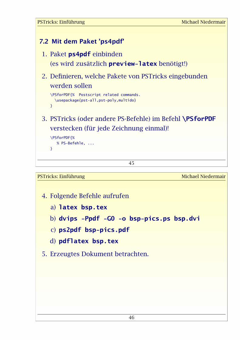
7.2 Mit dem Paket ’ps4pdf’
1. Paket ps4pdf einbinden
(es wird zusätzlich preview-latex benötigt!)
2. Definieren, welche Pakete von PSTricks eingebunden
werden sollen\PSforPDF{% Postscript related commands.
\usepackage{pst-all,pst-poly,multido}
}
3. PSTricks (oder andere PS-Befehle) im Befehl \PSforPDF
verstecken (für jede Zeichnung einmal)!
\PSforPDF{%
% PS-Befehle, ...
}
PSTricks: Einführung Michael Niedermair
46
4. Folgende Befehle aufrufen
a) latex bsp.tex
b) dvips -Ppdf -G0 -o bsp-pics.ps bsp.dvi
c) ps2pdf bsp-pics.pdf
d) pdflatex bsp.tex
5. Erzeugtes Dokument betrachten.
PSTricks: Einführung Michael Niedermair
47
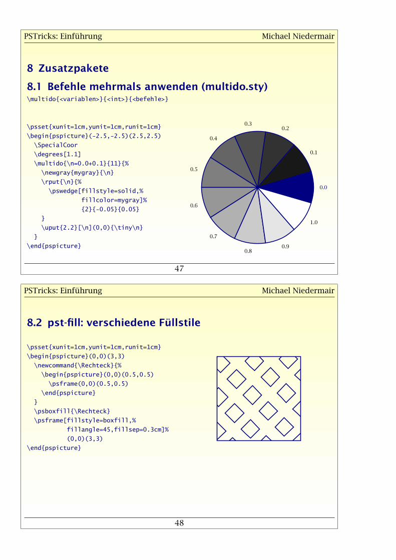
8 Zusatzpakete
8.1 Befehle mehrmals anwenden (multido.sty)\multido{<variablen>}{<int>}{<befehle>}
\psset{xunit=1cm,yunit=1cm,runit=1cm}
\begin{pspicture}(-2.5,-2.5)(2.5,2.5)
\SpecialCoor
\degrees[1.1]
\multido{\n=0.0+0.1}{11}{%
\newgray{mygray}{\n}
\rput{\n}{%
\pswedge[fillstyle=solid,%
fillcolor=mygray]%
{2}{-0.05}{0.05}
}
\uput{2.2}[\n](0,0){\tiny\n}
}
\end{pspicture}
0.0
0.1
0.20.3
0.4
0.5
0.6
0.7
0.80.9
1.0
PSTricks: Einführung Michael Niedermair
48
8.2 pst-fill: verschiedene Füllstile
\psset{xunit=1cm,yunit=1cm,runit=1cm}
\begin{pspicture}(0,0)(3,3)
\newcommand{\Rechteck}{%
\begin{pspicture}(0,0)(0.5,0.5)
\psframe(0,0)(0.5,0.5)
\end{pspicture}
}
\psboxfill{\Rechteck}
\psframe[fillstyle=boxfill,%
fillangle=45,fillsep=0.3cm]%
(0,0)(3,3)
\end{pspicture}
PSTricks: Einführung Michael Niedermair
49
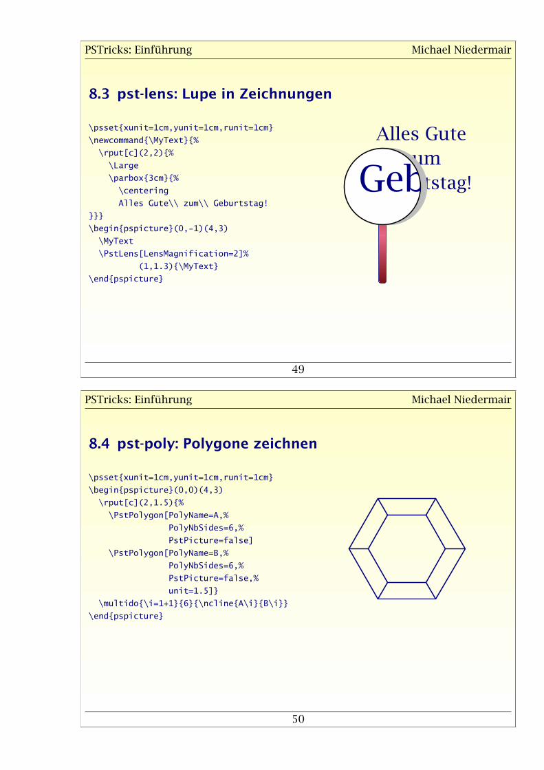
8.3 pst-lens: Lupe in Zeichnungen
\psset{xunit=1cm,yunit=1cm,runit=1cm}
\newcommand{\MyText}{%
\rput[c](2,2){%
\Large
\parbox{3cm}{%
\centering
Alles Gute\\ zum\\ Geburtstag!
}}}
\begin{pspicture}(0,-1)(4,3)
\MyText
\PstLens[LensMagnification=2]%
(1,1.3){\MyText}
\end{pspicture}
Alles Gute
zum
Geburtstag!
zum
Geburtstag!
PSTricks: Einführung Michael Niedermair
50
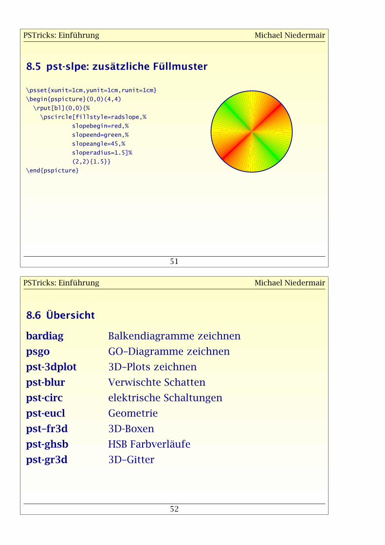
8.4 pst-poly: Polygone zeichnen
\psset{xunit=1cm,yunit=1cm,runit=1cm}
\begin{pspicture}(0,0)(4,3)
\rput[c](2,1.5){%
\PstPolygon[PolyName=A,%
PolyNbSides=6,%
PstPicture=false]
\PstPolygon[PolyName=B,%
PolyNbSides=6,%
PstPicture=false,%
unit=1.5]}
\multido{\i=1+1}{6}{\ncline{A\i}{B\i}}
\end{pspicture}
PSTricks: Einführung Michael Niedermair
51
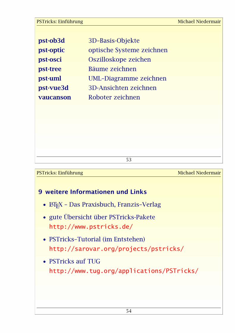
8.5 pst-slpe: zusätzliche Füllmuster
\psset{xunit=1cm,yunit=1cm,runit=1cm}
\begin{pspicture}(0,0)(4,4)
\rput[bl](0,0){%
\pscircle[fillstyle=radslope,%
slopebegin=red,%
slopeend=green,%
slopeangle=45,%
sloperadius=1.5]%
(2,2){1.5}}
\end{pspicture}
PSTricks: Einführung Michael Niedermair
52
8.6 Übersicht
bardiag Balkendiagramme zeichnen
psgo GO–Diagramme zeichnen
pst-3dplot 3D–Plots zeichnen
pst-blur Verwischte Schatten
pst-circ elektrische Schaltungen
pst-eucl Geometrie
pst–fr3d 3D-Boxen
pst-ghsb HSB Farbverläufe
pst-gr3d 3D–Gitter
PSTricks: Einführung Michael Niedermair
53
pst-ob3d 3D–Basis-Objekte
pst-optic optische Systeme zeichnen
pst-osci Oszilloskope zeichen
pst-tree Bäume zeichnen
pst-uml UML–Diagramme zeichnen
pst-vue3d 3D-Ansichten zeichnen
vaucanson Roboter zeichnen
PSTricks: Einführung Michael Niedermair
54
9 weitere Informationen und Links
• LATEX – Das Praxisbuch, Franzis–Verlag
• gute Übersicht über PSTricks-Pakete
http://www.pstricks.de/
• PSTricks–Tutorial (im Entstehen)
http://sarovar.org/projects/pstricks/
• PSTricks auf TUG
http://www.tug.org/applications/PSTricks/
PSTricks: Einführung Michael Niedermair
55
Fragen?