loeblatt06EI1-EIplus1-EPplus1

7/30/2019 loeblatt06EI1-EIplus1-EPplus1

http://slidepdf.com/reader/full/loeblatt06ei1-eiplus1-epplus1 1/8

1

HochschuleMathematik

Sem. EI1, EI-plus1, EP-plus1 Prof. Dr. ErhardtOffenburg Übungsblatt Nr. 6

WS 2012/13

Ausgabetermin: Donnerstag, 15. November 2012Abgabetermin: Donnerstag, 22. November 2012, Beginn 3. Stunde

Ergebnisse ohne Rechenweg werden mit 0P bewertet. Bitte, schreiben Sie leserlich und bedenken Sie, dass die TutorenIhre Ausführungen verstehen müssen.

Resultate, die nicht weitestgehend zusammengefasst sind, erhalten Punkteabzug!

Aufgabe 1 (18 Punkte)

Überlagern Sie die folgenden Schwingungen:a) u1(t) = 75 V cos(ωt + π/7), u2(t) = 80 V sin(ωt − 3/2)b) f 1(t) = 15 cm cos(ωt + 0.25), f 2(t) = 12 cm sin(ωt + 1.25)c) i1(t) = 0.5 A sin(ωt + π/6), i2(t) = 1.2 A cos(ωt + π/3),

i3(t) = 0.8 A sin(ωt − 5π/6)

Addieren Sie jeweils die Schwingungen rechnerisch aus ihrer Pfeildarstellung. Zeichnen Sie anschließend jeweilsfür a), b) und c) die Einzelschwingungen und die überlagerten Schwingungen mit Hilfe eines Plotprogramms in ein

Diagramm (ω = 2πf; f=50 Hz). Per Hand erstellte Zeichnungen werden nicht gewertet.


Zeigen Sie, dass gilt:

a) sinx · sin y =1

2cos(x− y)−

1

2cos(x + y) b) cosx · sin y =

1

2sin(x + y) −

1

2sin(x− y)

c) cosx · cos y =1

2cos(x + y) +

1

2cos(x − y) d) tanx · tan y =

cos(x− y)− cos(x + y)

cos(x− y) + cos(x + y)


Zeigen Sie mit Hilfe der Additionstheoreme für trigonometrische Funktionen:

a) sin(2α) = 2 sinα cosα b) cos(2α) = cos2 α− sin2 α

c) tan(2α) =2tanα

1 − tan2 αd) cot(2α) =

cot2 α− 1

2cotα


Zeigen Sie mit Hilfe der Additionstheoreme für Hyperbelfunktionen:

a) sinh(2x) = 2 sinhx coshx b) cosh(2x) = cosh2

x + sinh2

x

c) tanh(2x) =2 tanhx

1 + tanh2 xd) coth(2x) =

coth2 x + 1

2 cothx


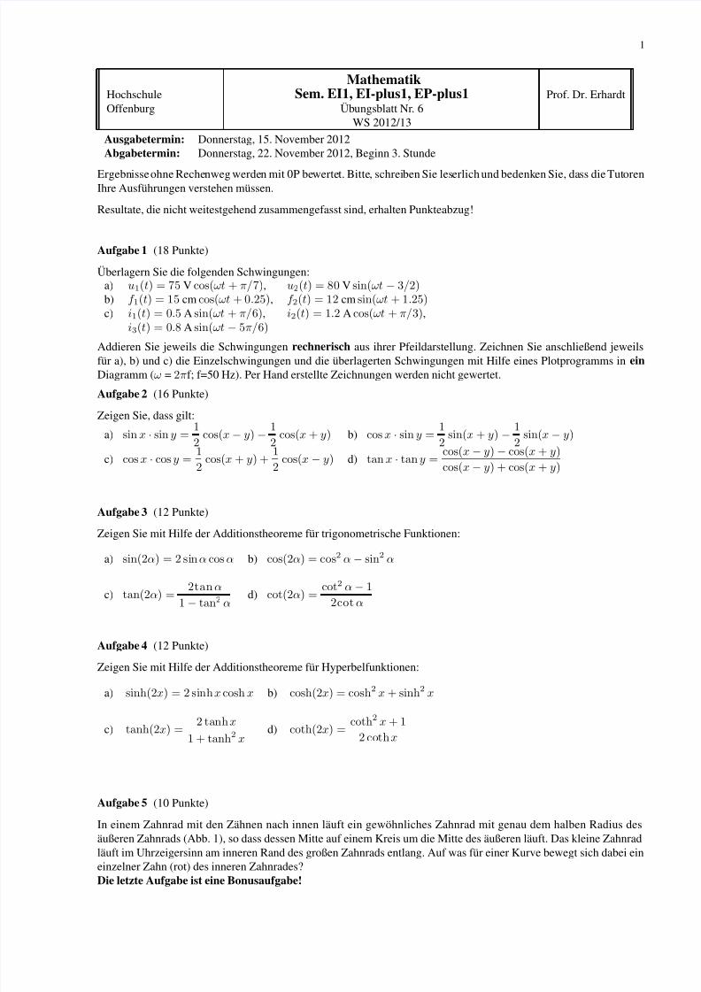
In einem Zahnrad mit den Zähnen nach innen läuft ein gewöhnliches Zahnrad mit genau dem halben Radius desäußeren Zahnrads (Abb. 1), so dass dessen Mitte auf einem Kreis um die Mitte des äußeren läuft. Das kleine Zahnradläuft im Uhrzeigersinn am inneren Rand des großen Zahnrads entlang. Auf was für einer Kurve bewegt sich dabei ein

einzelner Zahn (rot) des inneren Zahnrades?Die letzte Aufgabe ist eine Bonusaufgabe!



2

Abbildung 1: Aufgabe 5: Zwei Zahnräder. Das kleine Zahnrad läuft im Uhrzeigersinn am inneren Rand des großen Zahnradsentlang



3

Lösung 1

Die Überlagerung von Schwingungen kann man nach den Formeln

Ages = A21 + A2

2 + 2A1A2 cos(ϕ2 − ϕ1)

tanϕges =

A1 sinϕ1 + A2 sinϕ2

A1 cosϕ1 + A2 cosϕ2

oder, was insbesondere bei der Addition von mehr als 2 Schwingungen hilfreich ist, über die Komponenten:

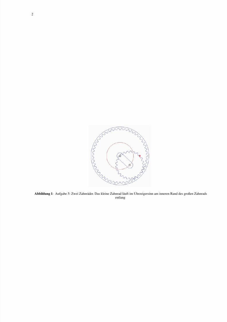
a)

u1(t) = 75 V cos(ωt + π/7)

= 75 V sin

ωt +

9π

14

u2(t) = 80 V sin(ωt − 3/2)

Spannung Amplitude u0 Phase ϕ horiz. Komponente ux vertik. Komponente uy

u1 75 V9π

14-32.54 67.57

u2 80 V −3

25.66 -79.80

uges -26.88 -12.23

Amplitude: u0ges = u2xges + u2yges = 29.53 V

Phase: ϕges = arctan

uyges

uxges

= 3.569

Funktionsgleichung: uges(t) = 29.53 V sin(ωt + 3.569)V

Zeichnung siehe Abb. 2

u(t) [V]

t [ms]

-80.0

-60.0

-40.0

-20.0

0.0

20.0

40.0

60.0

80.0

-20.0 -15.0 -10.0 -5.0 0.0 5.0 10.0 15.0

u1(x)u2(x)

u1(x)+u2(x)

Abbildung 2: Lösung 1: a) u1(t), u2(t) und u1(t) + u2(t)

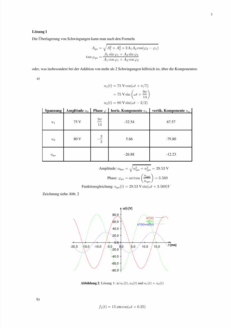
b)

f 1(t) = 15 cm cos(ωt + 0.25)



4

= 15 cm sinωt + 0.25 +

π

2

f 2(t) = 12 cm sin(ωt + 1.25)

Funktion Amplitude f 0 Phase ϕ horiz. Komponente f x vertik. Komponente f y

f 1 15 V 0.25 +π

2 -3.71 14.53

f 2 12 V 1.25 3.78 11.39

f ges 0.07 25.92

Amplitude: f 0ges = f 2xges + f 2yges = 25.92 cm

Phase: ϕges = arctanf yges

f xges

= 1.568 ≈

π

2

Funktionsgleichung: f ges(t) = 25.92 cm sin(ωt + 1.568)


f(t) [cm]

t [ms]

-30.0

-20.0

-10.0

0.0

10.0

20.0

30.0

-20.0 -15.0 -10.0 -5.0 0.0 5.0 10.0 15.0

f1(t)f2(t)

f1(t)+f2(t)

Abbildung 3: Lösung 1: b) f 1(t), f 2(t) und f 1(t) + f 2(t)

c)

i1(t) = 0.5 A sinωt +

π

6

i2(t) = 1.2 A cosωt +π

3= 1.2 A sin

ωt +

5π

6

i3(t) = 0.8 A sin

ωt −

5π

6



5

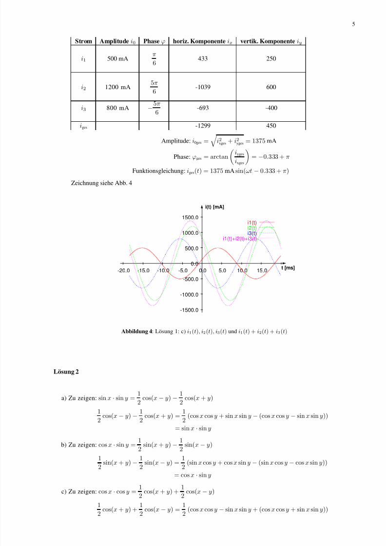
Strom Amplitude i0 Phase ϕ horiz. Komponente ix vertik. Komponente iy

i1 500 mAπ

6433 250

i2 1200 mA5π

6-1039 600

i3 800 mA −5π

6-693 -400

iges -1299 450

Amplitude: i0ges = i2xges + i2yges = 1375 mA

Phase: ϕges = arctan

iyges

ixges

= −0.333 + π

Funktionsgleichung: iges(t) = 1375 mA sin(ωt − 0.333 + π)


i(t) [mA]

t [ms]

-1500.0

-1000.0

-500.0

0.0

500.0

1000.0

1500.0

-20.0 -15.0 -10.0 -5.0 0.0 5.0 10.0 15.0

i1(t)i2(t)i3(t)

i1(t)+i2(t)+i3(t)

Abbildung 4: Lösung 1: c) i1(t), i2(t), i3(t) und i1(t) + i2(t) + i3(t)

Lösung 2

a) Zu zeigen: sinx · sin y =1

2cos(x− y)−

1

2cos(x + y)

1

2cos(x− y)−

1

2cos(x + y) =

1

2(cosx cosy + sinx sin y − (cosx cos y − sinx sin y))

= sinx · sin y

b) Zu zeigen: cosx · sin y =1

2sin(x + y)−

1

2sin(x− y)

1

2sin(x + y)−

1

2sin(x− y) =

1

2(sinx cos y + cosx sin y − (sinx cos y − cosx sin y))

= cosx·

sin y

c) Zu zeigen: cosx · cos y =1

2cos(x + y) +

1

2cos(x− y)

1

2cos(x + y) +

1

2cos(x − y) =

1

2(cosx cosy − sinx sin y + (cosx cos y + sinx sin y))



6

= cosx · cos y

d) Zu zeigen: tanx · tan y =cos(x− y)− cos(x + y)

cos(x− y) + cos(x + y)

cos(x− y)− cos(x + y)

cos(x− y) + cos(x + y)=

cosx cos y + sinx sin y − (cos x cos y − sinx sin y)

cosx cos y + sinx sin y + cosx cos y − sinx sin y

= 2sinx sin y2cosx cos y

= tanx · tan y



7

Lösung 3

a) Zu zeigen: sin(2α) = cosα sinα + sinα cosα.

sin(2α) = sin(α + α)

= cosα sinα + sinα cosα = sinα cosα

b) Zu zeigen: cos(α + α) = cosα cosα− sinα sinα.

cos(2α) = cos(α + α)

= cosα cosα− sinα sinα = cos2 α− sin2 α

c) Zu zeigen: tan(2α) =2tanα

1 − tan2 α.

tan(2α) = tan(α + α)

=tanα + tanα

1 − tanα tanα=

2tanα

1 − tan2 α

d) Zu zeigen: cot(2α) =cot2 α− 1

2cotα.

cot(2α) = cot(α + α)

=cotα cotα− 1

cotα + cotα=

cot2 α− 1

2cotα

Lösung 4

a) Zu zeigen: sinh(x1 ± x2) = sinhx1 · coshx2 ± coshx1 · sinhx2

sinhx1 · coshx2 ± coshx1 · sinhx2 =1

4

(ex1 − e−x1)(ex2 + e−x2)± (ex1 + e−x1)(ex2 − e−x2)

=1

4(ex1+x2 + ex1−x2 − e−x1+x2 − e−(x1+x2)

± ex1+x2 ∓ ex1−x2 ± e−x1+x2 ∓ e−(x1+x2))

alle + ausgewertet: =1

4

2ex1+x2 − 2e−(x1+x2)

= sinh(x1 + x2)

alle - ausgewertet: =

1

4

2ex1−x2

− 2e−(x1−x2)

= sinh(x1 − x2)

b) Zu zeigen: cosh(x1 ± x2) = coshx1 · coshx2 ± sinhx1 · sinhx2

coshx1 · coshx2 ± coshx1 · cosx2 =1

4

(ex1 + e−x1)(ex2 + e−x2)± (ex1 − e−x1)(ex2 − e−x2)

=1

4(ex1+x2 + ex1−x2 + e−x1+x2 + e−(x1+x2)

± ex1+x2 ∓ ex1−x2 ∓ e−x1+x2 ± e−(x1+x2))

alle + ausgewertet: =1

4 2ex1+x2 + 2e−(x1+x2)= cosh(x1 + x2)

alle - ausgewertet: =1

4

2ex1−x2 + 2e−(x1−x2)

= cosh(x1 − x2)



8

c) Zu zeigen: tanh(x1 ± x2) =tanhx1 ± tanhx2

1 ± tanhx1 · tanhx2

tanh(x1 ± x2) =sinh(x1 ± x2)

cosh(x1 ± x2)

=sinhx1 · coshx2 ± coshx1 · sinhx2coshx1 · coshx2 ± sinhx1 · sinhx2

=tanhx1 ± tanhx2

1 ± tanhx1 · tanhx2(mit coshx1 · coshx2 gekürzt)

d) Zu zeigen: coth(x1 ± x2) =1± cothx1 · cothx2

cothx1 ± cothx2

coth(x1 ± x2) =cosh(x1 ± x2)

sinh(x1 ± x2)

=coshx1 · coshx2 ± sinhx1 · sinhx2sinhx1 · coshx2 ± coshx1 · sinhx2

=cothx1 · cothx2 ± 1

cothx2± cothx

1

(mit sinhx1 · sinhx2 gekürzt)

=1 ± cothx1 · cothx2

cothx1 ± cothx2

Lösung 5

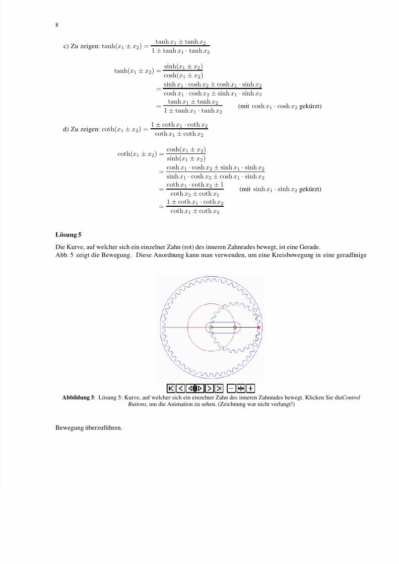
Die Kurve, auf welcher sich ein einzelner Zahn (rot) des inneren Zahnrades bewegt, ist eine Gerade.Abb. 5 zeigt die Bewegung. Diese Anordnung kann man verwenden, um eine Kreisbewegung in eine geradlinige

Abbildung 5: Lösung 5: Kurve, auf welcher sich ein einzelner Zahn des inneren Zahnrades bewegt. Klicken Sie die Control

Buttons, um die Animation zu sehen. (Zeichnung war nicht verlangt!)

Bewegung überzuführen.

Documents

loeblatt06EI1-EIplus1-EPplus1