PF-FLO REFERENCE TEST

AT THE

MARTIN-LUTHER UNIVERSITY HALLE-WITTENBERG

Martin-Luther-Universität Halle-Wittenberg AMC Power – PROMECON

Fachbereich Ingenieurwissenschaften 1050 Hopper Avenue

Lehrstuhl für Mechanische Verfahrenstechnik Santa Rosa, California 95403

06099 Halle (Saale) U.S.A.

Germany

PF-FLO REFERENCE TEST AT THE MARTIN-LUTHER UNIVERSITYHALLE-WITTENBERG

CONTENTS Page

1. Introduction..................................................................................................... 12. Description of the Test Facilities..................................................................... 3

2.1 The Testing Plant ................................................................................... 32.2 The Pf-FLO Mass Flow Measurement.................................................... 4

2.2.1 Density measurement.................................................................. 42.2.2 Velocity measurement ................................................................. 52.2.3 Calculation of the Mass Flow....................................................... 6

2.3 Pf-FLO Test Configuration...................................................................... 62.4 The Test Medium.................................................................................... 82.5 Feeder Calibration .................................................................................. 9

3. Testing Procedure .......................................................................................... 114. Results ........................................................................................................... 14

4.1 Pf-FLO Measurement Accuracy ............................................................. 144.1.1 Absolute Deviation....................................................................... 154.1.2 Repeatability ................................................................................ 16

4.2 Influence of the Particle Size .................................................................. 174.2.1 Velocity Measurement ................................................................. 174.2.2 Density Measurement.................................................................. 194.2.3 Mass flow measurement .............................................................. 20

5. Abstract .......................................................................................................... 23

Figures PageFig. 2.1: Schematic drawing of the test plant ............................................................. 3

Fig. 3.1: Range of pf-concentrations based on feeder mass flow and transport airflow .............................................................................................................. 11

Fig. 3.2: Density measurement .................................................................................. 12

Fig. 3.3: Velocity measurement ................................................................................. 12

Fig. 3.4: Resulting mass flow and feeder signal......................................................... 12

Fig. 3.5: Mass flow of feeder versus Pf-FLO.............................................................. 12

Fig. 4.1: Evaluation of all test runs with 66 / 225 µm particles ................................... 14

Fig. 4.2: Repeatability of channel 0 for 66 - 225 µm particles .................................... 15

Fig. 4.3 Averaged particle velocities at channel 0..................................................... 17

Fig. 4.4: Acceleration along the test duct of the 225 µm particles.............................. 18

Fig. 4.5: Influence of the mass flow on the velocity of the particle mix in Test IV-VI .. 18

Fig. 4.6: Density measurement with 66 µm particles Test V. ..................................... 19

Fig. 4.7: Density measurement with 225 µm particles Test I ..................................... 19

Fig. 4.8: Influence of the particle size on the Pf-FLO measurement .......................... 20

Fig. 4.9: Estimated deviation by modeled particle size distribution............................ 22

Tables PageTable 2.1:Bulk density and frequency shift for fixed-bed powder of pulverized black

coal and glass particles................................................................................ 8

Table 3.1:Test run number for each particle size......................................................... 12

Table 4.1:Standard deviation and mean error for individual particle fractions ............. 15

Table 4.2:Standard deviation of the individual channels with 66 µm particles ............. 16

Table 4.3:Standard deviation of the individual channels with 225 µm particles ........... 16

Table 4.4:Standard deviation of the individual channels with 66-225 µm particle mix . 16

Table 4.5:Ratio of arbitrary units to mass and the resulting mass frequency factor kfd

for each particle fraction............................................................................... 21

1. Introduction

Measurement of particle concentration or mass flow rate in pipeline systems (i.e.pneumatic conveying) is essential for numerous technical applications, such asconveying of pulverized coal in power plants or conveying systems in cementfactories. Of major importance is the detection of the particulate flow in the entirecross-section of a pipe. In the past this has generally only been achieved in pipeelements where the particulate concentration is homogeneously distributed over theentire cross-section. For such a measurement different techniques are available,namely extractive methods utilizing probes and non-extractive methods employingelectromagnetic waves or particle charging. From the first inspection an isokineticsampling probe seems to be the simplest approach, however, in order to measurethe particulate flux in the entire pipe section it is necessary to systematically positionthe extraction probe at defined locations across the entire pipe cross-section. Due toprobe erosion damage, extractive sampling is only suitable for periodicmeasurement. For continuous measurement, non-extractive methods are morefavorable, where the sensing instrumentation is mounted in-situ. One approach is thedetection of the electrostatic charge of moving particles. Unfortunately, the resultingsignal is not only affected by particle concentration, but also by gas temperature andparticle velocity. The method used for the investigation documented in this report isbased on utilizing microwaves emitted and detected by screw-in sensors. Thegenerated microwave field covers the entire pipe cross-section and hence allows thedetermination of the averaged particle concentration over that cross-section. Theprinciple of the method will be outlined below.

The microwave based experiments were conducted on an air-particle flow loopestablished at the Lehrstuhl für Mechanische Verfahrenstechnik of the Martin-LutherUniversity Halle-Wittenberg. In order to consider different conveying conditions,probes were installed at multiple locations of the conveying pipe, namely in anupward flow with almost homogeneous dust distribution, behind a vertical-horizontalbend where roping is likely to occur, and in an almost fully developed state of ahorizontal pipe. The particle introduction was achieved using a calibrated screwfeeder, which also allowed the comparison of the particulate mass flow with the resultfrom the microwave instrument. Since the handling of pulverized coal could not besafely performed at the test facility, spherical glass beads of two different meandiameters were used as coal substitutes. It is acknowledged that the differentmaterial density and particle shape of the glass particles results in a slightly differentconveying behavior, primarily in the form of lower particle velocities, but otherwisethe general flow behavior of coal and glass particle is extremely similar.

This report presents a description of the test facility and the measurement principle.The measurements are presented in comparison with the calibrated screw feeder,and a detailed discussion of the accuracy achieved with the microwave instrument isprovided.

2. Description of the Test Facilities

The reference test was carried out at the Merseburg test plant. The test facility isdesigned with a closed loop for the particle flow and an open end for the transport air.This arrangement ensures particle recycling via a cyclone back to the feeder withoutsignificant particle mass loss, for re-introduction at a controlled rate/concentration.For safety reasons the test plant was operated with glass beads of two differentdiameters instead of pulverized coal. Particle load and transport air velocity werevaried during the test series in a range simulating that which naturally occurs withpneumatically transported coal (see test matrix, Figure 3.1 and Table 3.1).

2.1 The Testing Plant

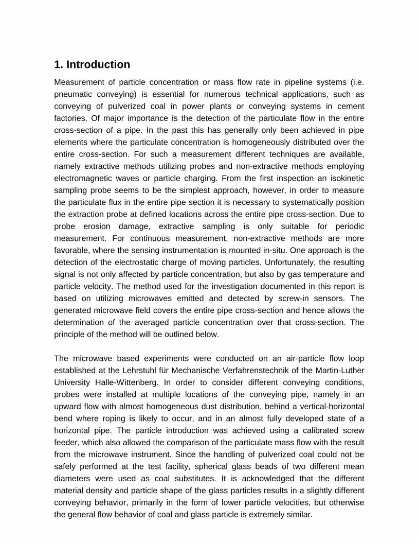
The test duct layout is drawn in Figure 2.1. Two rotary piston blowers, operating inparallel and controlled by fan speed frequency converters, providing a velocity rangeof about 46 to 92 ft³/s for the transport air.

Cyclone

Rotary Valve

Screw Feeder

Bagfilter

Ch 3 Ch 2

Ch 1

Ch 0

Hopper

Air Outlet

16.5 ft.

10 ft. Air

Inle

t

Fig. 2.1: Schematic drawing of the test plant

The particles are introduced to the airflow by a screw feeder, transported through thepipe and separated in a cyclone. Out of the cyclone the separated particles are fed

by a rotary valve back into the hopper of the screw feeder. The transport air isexhausted through a bag filter.

The screw feeder is frequency controlled over a range of 0 – 350 rpm. The horizontalrun downstream of the feeder has a rectangular cross section, whereas the verticaland the upper horizontal pipes where the Pf-FLO measurements are located areround pipes having an inner diameter of 4.86”.

The airflow velocity is measured by a multi-point Pitot probe positioned upstream ofthe feeder. In addition, the airflow static pressure and temperature are alsomonitored.

2.2 The Pf-FLO Mass Flow Measurement

The Pf-FLO system independently measures the density and velocity of pulverizedfuel in a two-phase flow. After a “zero” calibration of the empty transport pipe isperformed for the density measurement process, absolute mass flow can becalculated using the product of the separate density and coal velocity signals.

2.2.1 Density measurement

Using the pipe as a wave-guide, the particulate concentration or density is measuredwith transmitted microwaves that cover the full cross section of the pipe. Startingwith the known microwave transmission characteristic determined during empty pipezeroing, the varying dielectric load caused by changing pulverized fuel (pf)concentrations produces a measurable frequency shift. The basics of thismeasurement can be described as follows1):

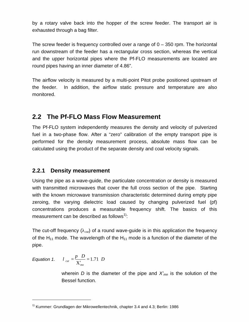
The cut-off frequency (λcut) of a round wave-guide is in this application the frequencyof the H11 mode. The wavelength of the H11 mode is a function of the diameter of thepipe.

Equation 1.

wherein D is the diameter of the pipe and X’mn is the solution of theBessel function.

1) Kummer: Grundlagen der Mikrowellentechnik, chapter 3.4 and 4.3; Berlin: 1986

DD

mncut ⋅=

Χ′⋅

= 71.1π

λ

The frequency (ƒ) of the H11 mode depends on the dielectric εr and the magnetic µr

properties of the volume in the wave-guide.

Equation 2. where c is the constant for the speed of light

An unloaded pipe filled with air has a εr of 1 and a µr of 1. Hard coal has an εr of 4and µr of 1. The volumetric ratio of pulverized coal to air at a coal concentration of0.0312 lb/ft³ is 1 to 2500. Since the resulting εr changes between loaded and emptypipe in terms of 1/2500 the series expansion of Equation 2 can be used with its linearterm. This gives a linear relation between the frequency and pf load within theconcentration range typically found in coal fired power plants.

The Pf-FLO system couples microwaves in the range of the cut-off frequency into apipe section using a pair of sensors, one sensor functioning as the transmitter and asecond sensor as the receiver. The exact frequency of the H11 mode is calculated byscanning the transmitted microwave signal amplitudes.

A change in the concentration of pf in a given pipe changes the measured microwavefrequency: The higher the concentration, the lower the frequency. The frequency shiftcaused by the pf is calculated by subtracting the frequency fε of the loaded pipe fromthe frequency f0 of the empty pipe. This frequency shift is transformed into a densitysignal (ρ) by the frequency density factor kfd.

Equation 3.

Where f0 is determined by the empty pipe zeroing process.

Changes in pipe diameter caused by temperature do affect the measured frequency.Temperature compensation of the measured frequency uses the pipe surfacetemperature and the linear expansion factor for that pipe material.

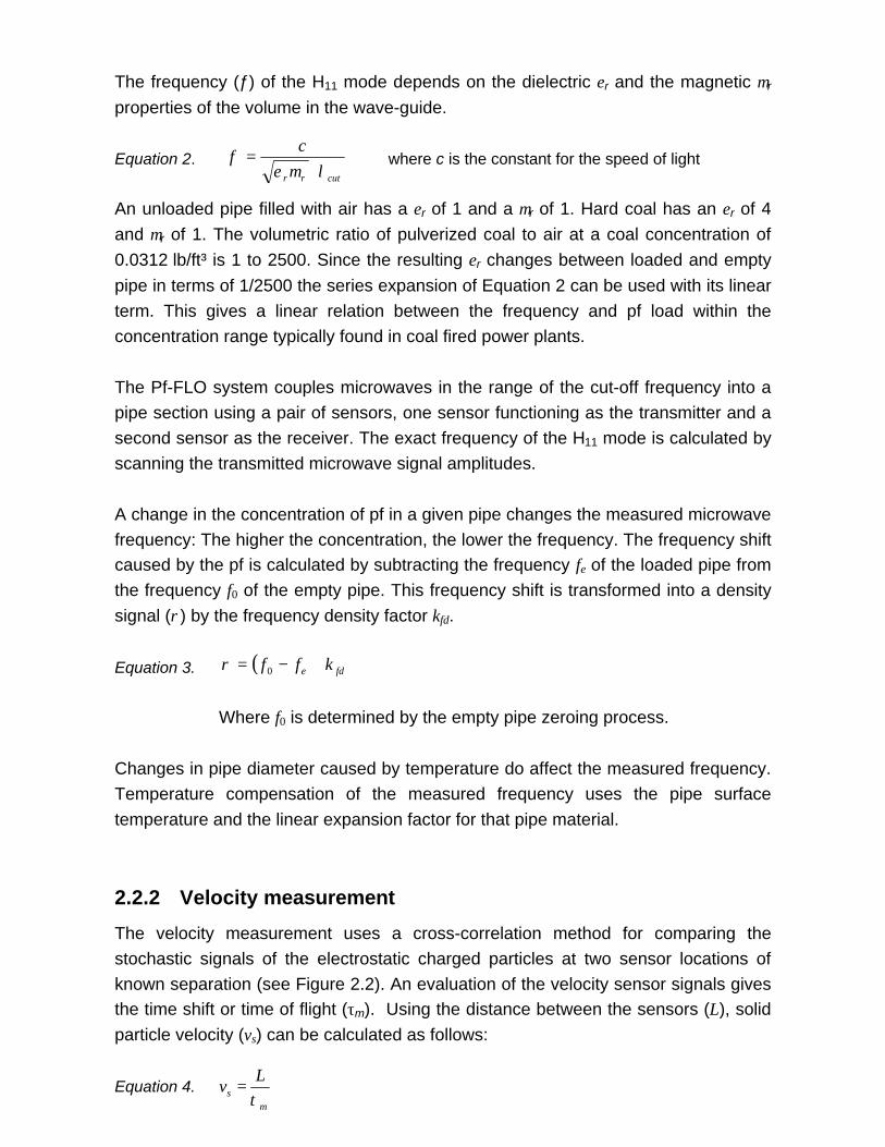
2.2.2 Velocity measurement

The velocity measurement uses a cross-correlation method for comparing thestochastic signals of the electrostatic charged particles at two sensor locations ofknown separation (see Figure 2.2). An evaluation of the velocity sensor signals givesthe time shift or time of flight (τm). Using the distance between the sensors (L), solidparticle velocity (vs) can be calculated as follows:

Equation 4.

( ) fdkff ⋅−= ερ 0

cutrr

cf

λµε ⋅=

ms

Lv

τ=

By using this method only particle velocity is measured, which in most instancesdiffers from and is slower than the transport air velocity in a two-phase flow. Thisdifference, or velocity slip, is a function of such factors as pipe configuration, specificweight and size of particles.

Signal 1

Signal 2

Cross-correlation

Fig. 2.2: Velocity measurement principle: signals and

resulting cross-correlation function

2.2.3 Calculation of the Mass Flow

The mass flow is calculated from the density and the particulate velocity

measurement as follows:

Equation 5.

The Pf-FLO system is calibrated to a known mass flow of the mill or pipe by adjustingthe frequency density factor kfd in Equation 3, which in turn depends on the pipediameter. The factor kfd is kept constant for all pipes with the same diameter.

2.3 Pf-FLO Test Configuration

The 4.86” diameter test duct pipe has a cut-off frequency of approximately 1.4 GHz.The standard microwave generating unit of the Pf-FLO system has been selected toprovide frequencies up to only a 1 GHz level required for the range of larger coal pipe

svdtdm

⋅= ρ

dtdm

Velocity = L / τm

5.25 D

rod

sensor

0.87 D 1.0 D 0.75 D 0.75 D 1.0 D 0.87 D

dtdm

sizes found in power plants. For the test runs conducted it was necessary to replacethe standard model generator with a similar model having an extended frequencyrange of up to 2.0 GHz.

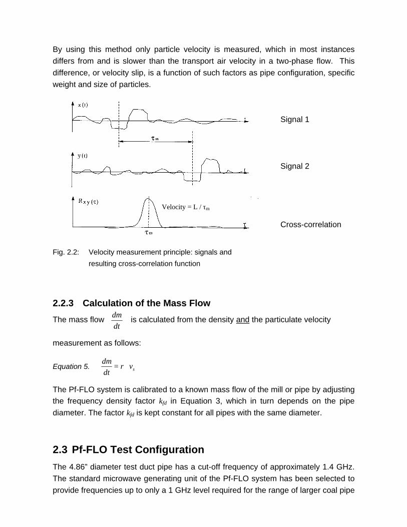
Corresponding to the smaller inner diameter of the test duct, the sensor antenna wasalso scaled down in length. Distances between sensors and rods in the test runswere the standard distances based on a pipe having a diameter D, as show in Figure2.3.

Fig. 2.3: Arrangement of sensors and rods at individual measurement locations

The Pf-FLO system uses wear resistant Tungsten Carbide rods to keep thepropagation of the microwaves within the certain measurement zone of the pipe.Without the rods, the density measurement would be disturbed by reflected signalscaused by pipe bends, orifice plates, isolation valves, etc., located upstream and/ordownstream of the measurement zone. The optional fifth rod perpendicular to thesensors and located at their midpoint provides an additional signal short cut fordepressing the propagation of 90° polarized H11 modes.

Without knowing the actual mass frequency factor for the test pipe size, all channelswere initially set to

This factor was kept constant for all measurements in the test. The resulting units for

measured density (ρ) and mass flow are in arbitrary units [a.u.].

⋅=

mHza.u.

500fdk

2.4 The Test Medium

The test plant could not be used with black coal for safety reasons. Therefore, glassspheres were used, with such properties as particle size, dielectric constant, andelectrostatic charging similar to pulverized coal.

Typically 85 % – 95 % by weight of pulverized coal particles downstream of the mill’sclassifier are smaller than 90 µm and 0.3 % or less are bigger than 225 µm. The twoglass particle sizes of 66 µm and 225 µm used for this test represent the mainfraction and the biggest possible size fraction of particles in coal pipes.

The manufacturer of the glass beads specifies a glass density of 158.6 lb/ft³ and an εr

of 2.28 at visible light. The εr may be slightly different for microwaves due todispersion.

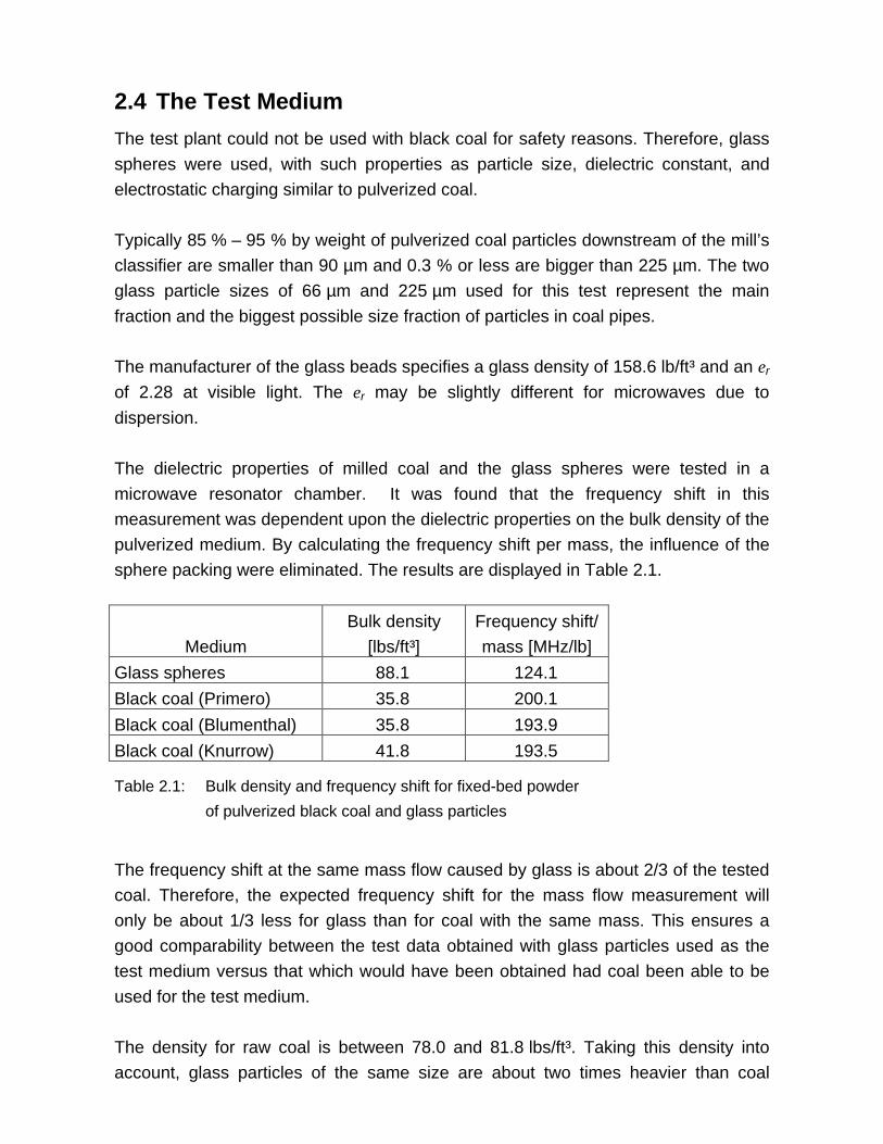
The dielectric properties of milled coal and the glass spheres were tested in amicrowave resonator chamber. It was found that the frequency shift in thismeasurement was dependent upon the dielectric properties on the bulk density of thepulverized medium. By calculating the frequency shift per mass, the influence of thesphere packing were eliminated. The results are displayed in Table 2.1.

MediumBulk density

[lbs/ft³]Frequency shift/mass [MHz/lb]

Glass spheres 88.1 124.1Black coal (Primero) 35.8 200.1Black coal (Blumenthal) 35.8 193.9Black coal (Knurrow) 41.8 193.5

Table 2.1: Bulk density and frequency shift for fixed-bed powder

of pulverized black coal and glass particles

The frequency shift at the same mass flow caused by glass is about 2/3 of the testedcoal. Therefore, the expected frequency shift for the mass flow measurement willonly be about 1/3 less for glass than for coal with the same mass. This ensures agood comparability between the test data obtained with glass particles used as thetest medium versus that which would have been obtained had coal been able to beused for the test medium.

The density for raw coal is between 78.0 and 81.8 lbs/ft³. Taking this density intoaccount, glass particles of the same size are about two times heavier than coal

particles. The weight differential plus the shape of the particles, spherical for glassand polyhedral for coal, give glass aerodynamic properties which result in a greatervelocity differential or slip between the airflow and the glass particles.

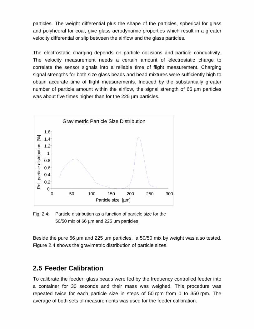
The electrostatic charging depends on particle collisions and particle conductivity.The velocity measurement needs a certain amount of electrostatic charge tocorrelate the sensor signals into a reliable time of flight measurement. Chargingsignal strengths for both size glass beads and bead mixtures were sufficiently high toobtain accurate time of flight measurements. Induced by the substantially greaternumber of particle amount within the airflow, the signal strength of 66 µm particleswas about five times higher than for the 225 µm particles.

Gravimetric Particle Size Distribution

0

0.2

0.4

0.6

0.8

1

1.2

1.4

1.6

0 50 100 150 200 250 300Particle size [µm]

Rel

. par

ticle

dis

trib

utio

n [%

]

Fig. 2.4: Particle distribution as a function of particle size for the

50/50 mix of 66 µm and 225 µm particles

Beside the pure 66 µm and 225 µm particles, a 50/50 mix by weight was also tested.Figure 2.4 shows the gravimetric distribution of particle sizes.

2.5 Feeder Calibration

To calibrate the feeder, glass beads were fed by the frequency controlled feeder intoa container for 30 seconds and their mass was weighed. This procedure wasrepeated twice for each particle size in steps of 50 rpm from 0 to 350 rpm. Theaverage of both sets of measurements was used for the feeder calibration.

The repeatability of the feeder calibration was then tested by 10 individualmeasurements with the 66 µm particles at 150 rpm. They were all in the range of±0.9 % by weight.

This was acceptable since the aim of the tests was not to examine the characteristicsof the screw feeder. And with all four sensor locations measuring physically the sameairflow/particle mixture, any scattering of the feeder is eliminated as a commonvariable.

Feeder Calibration

0

.11

.22

.33

.44

.55

0 50 100 150 200 250 300 350 400

Feeder speed [rpm]

Mas

s flo

w [l

bs/s

]

66 – 225 µmmix225 µm

66 µm

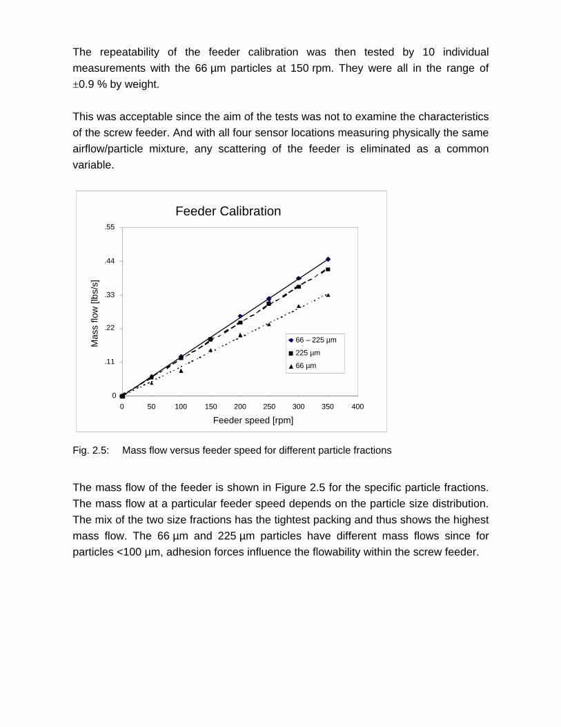
Fig. 2.5: Mass flow versus feeder speed for different particle fractions

The mass flow of the feeder is shown in Figure 2.5 for the specific particle fractions.The mass flow at a particular feeder speed depends on the particle size distribution.The mix of the two size fractions has the tightest packing and thus shows the highestmass flow. The 66 µm and 225 µm particles have different mass flows since forparticles <100 µm, adhesion forces influence the flowability within the screw feeder.

3. Testing Procedure

The test runs have been made under the aspect of realistic airflow velocities andparticle concentrations.

Within the capacity of the fan, three velocity levels were chosen at 72 ft/s, 82 ft/s, and92 ft/s, representing normal transport velocities in utility plants. With constant airvelocities the feeder speed was varied between 0 - 300 rpm in steps of 50 rpm.

Particle Concentration Range

0

0.006

0.013

0.019

0.025

0.031

0.037

0.044

0.050

0 50 100 150 200 250 300 350

Feeder speed [rpm]

Con

cent

ratio

n [lb

s/ft³

]

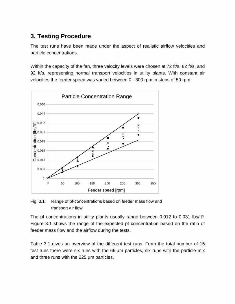
Fig. 3.1: Range of pf-concentrations based on feeder mass flow and

transport air flow

The pf concentrations in utility plants usually range between 0.012 to 0.031 lbs/ft³.Figure 3.1 shows the range of the expected pf concentration based on the ratio offeeder mass flow and the airflow during the tests.

Table 3.1 gives an overview of the different test runs: From the total number of 15test runs there were six runs with the 66 µm particles, six runs with the particle mixand three runs with the 225 µm particles.

Particle Size Test Numbers

66 µm I,VI II,V III,IV225 µm I II III66 - 225 µm mix I,IV II,V III, VI

72 ft/s 82 ft/s 92 ft/sGas Velocity

Table 3.1: Test run number for each particle size

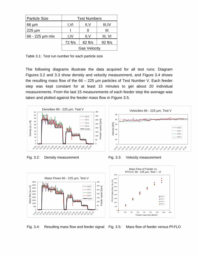
The following diagrams illustrate the data acquired for all test runs: DiagramFigures 3.2 and 3.3 show density and velocity measurement, and Figure 3.4 showsthe resulting mass flow of the 66 – 225 µm particles of Test Number V. Each feederstep was kept constant for at least 15 minutes to get about 20 individualmeasurements. From the last 15 measurements of each feeder step the average wastaken and plotted against the feeder mass flow in Figure 3.5.

0

6

12

18

24

30

36

42

48

54

61

13:04

13:1

2

13:20

13:2

9

13:37

13:4

613

:5414

:02

14:1

114

:1914

:28

14:3

614

:4414

:53

15:01

15:1

0

15:18

0

50

100

150

200

250

300

350

400

CH 0

CH 1

CH 2

CH 3

feeder

Densities 66 - 225 µm, Test V

Den

sity

[a.u

./ft]

Fee

der s

peed

[rpm

]

Fig. 3.2: Density measurement Fig. 3.3: Velocity measurement

0

500

1000

1500

2000

2500

3000

3500

4000

4500

13:0413:11

13:1913

:2613:

3413:41

13:4913:57

14:04

14:1214:19

14:2714

:3414:

4214:49

14:5715:05

15:12

15:20

0

50

100

150

200

250

300

350

CH 0

CH 1

CH 2

CH 3

feeder

Mas

s flo

w [a

.u./s

]

Mass Flows 66 - 225 µm, Test V

Feed

er s

peed

[rpm

]

Fig. 3.4: Resulting mass flow and feeder signal Fig. 3.5: Mass flow of feeder versus Pf-FLO

0

16

33

49

66

82

98

13:04

13:11

13:1

9

13:26

13:34

13:41

13:49

13:57

14:04

14:12

14:1

9

14:27

14:34

14:4

2

14:49

14:57

15:05

15:12

15:2

0

CH 0

CH 1

CH 2

CH 3

Velocities 66 - 225 µm, Test VVe

loci

ty [f

t/s]

Mass Flow of Feeder vs.Pf-FLO, 66 - 225 µm, Test I - VI

0

500

1000

1500

2000

2500

3000

3500

4000

4500

0 198 397 595 793 992 1190 1389 1587

CH 0

CH 1

CH 2

CH 3

Pf-F

LO M

ass

flow

[a.

u./s

]

Feeder mass flow [lbs/hr]

All test runs have been plotted as displayed in Figure 3.5. As there is only a constantfactor between [a.u./s] and [g/s], a unified y-axis scaling was used to help evaluatethe influence of different particle sizes (see also Figure 4.8).

4. Results

4.1 Pf-FLO Measurement Accuracy

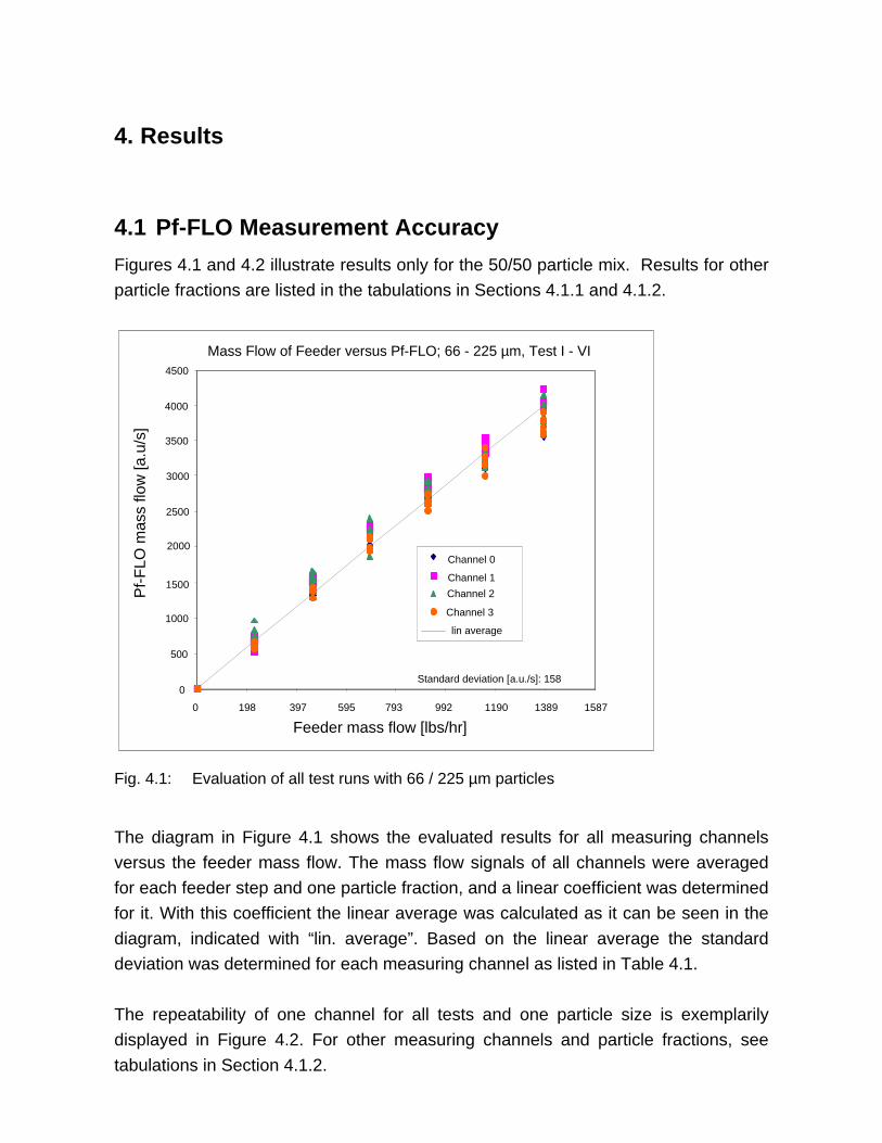
Figures 4.1 and 4.2 illustrate results only for the 50/50 particle mix. Results for otherparticle fractions are listed in the tabulations in Sections 4.1.1 and 4.1.2.

Mass Flow of Feeder versus Pf-FLO; 66 - 225 µm, Test I - VI

0

500

1000

1500

2000

2500

3000

3500

4000

4500

0 198 397 595 793 992 1190 1389 1587

Feeder mass flow [lbs/hr]

P

f-F

LO m

ass

flow

[a.u

/s]

Channel 0

Channel 1

Channel 2

Channel 3

lin average

Standard deviation [a.u./s]: 158

Fig. 4.1: Evaluation of all test runs with 66 / 225 µm particles

The diagram in Figure 4.1 shows the evaluated results for all measuring channelsversus the feeder mass flow. The mass flow signals of all channels were averagedfor each feeder step and one particle fraction, and a linear coefficient was determinedfor it. With this coefficient the linear average was calculated as it can be seen in thediagram, indicated with “lin. average”. Based on the linear average the standarddeviation was determined for each measuring channel as listed in Table 4.1.

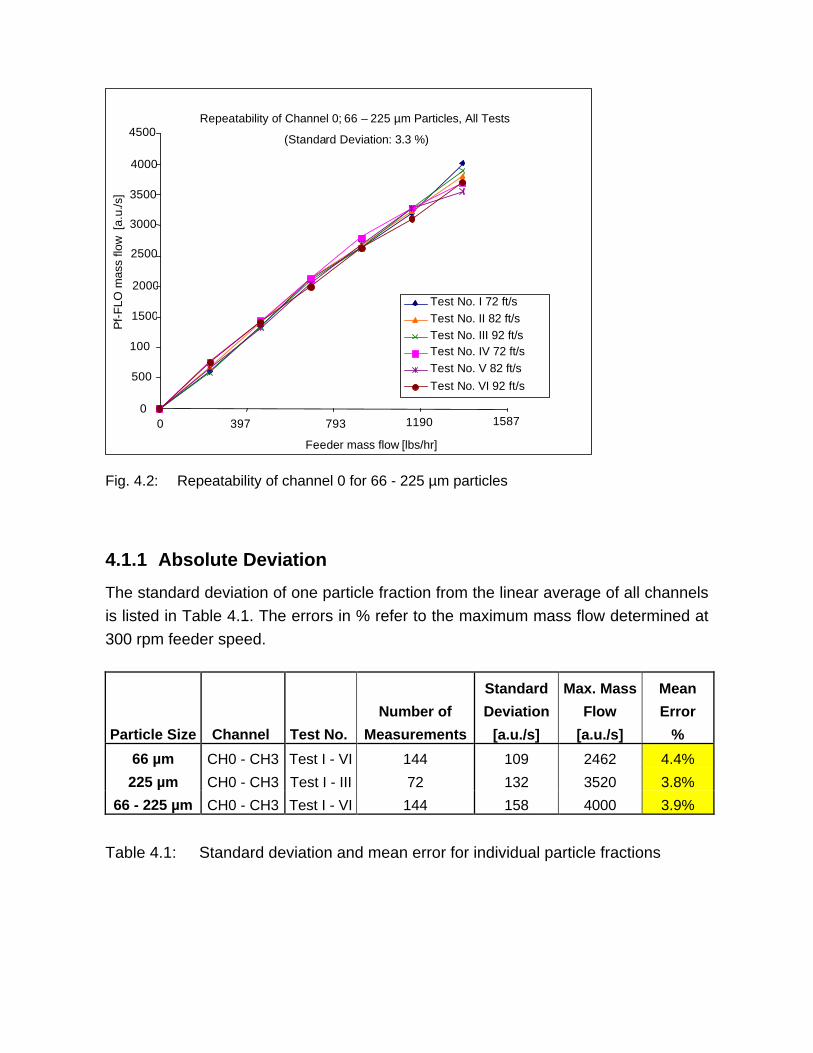
The repeatability of one channel for all tests and one particle size is exemplarilydisplayed in Figure 4.2. For other measuring channels and particle fractions, seetabulations in Section 4.1.2.

Repeatability of Channel 0; 66 – 225 µm Particles, All Tests

0

500

100

1500

2000

2500

3000

3500

4000

4500

0 397 793 1190 1587

Feeder mass flow [lbs/hr]

P

f-F

LO m

ass

flow

[a.

u./s

]

Test No. I 72 ft/s Test No. II 82 ft/s Test No. III 92 ft/s Test No. IV 72 ft/s Test No. V 82 ft/s Test No. VI 92 ft/s

(Standard Deviation: 3.3 %)

Fig. 4.2: Repeatability of channel 0 for 66 - 225 µm particles

4.1.1 Absolute Deviation

The standard deviation of one particle fraction from the linear average of all channelsis listed in Table 4.1. The errors in % refer to the maximum mass flow determined at300 rpm feeder speed.

Particle Size Channel Test No.

Number of

Measurements

Standard

Deviation

[a.u./s]

Max. Mass

Flow

[a.u./s]

Mean

Error

%

66 µm CH0 - CH3 Test I - VI 144 109 2462 4.4%

225 µm CH0 - CH3 Test I - III 72 132 3520 3.8%

66 - 225 µm CH0 - CH3 Test I - VI 144 158 4000 3.9%

Table 4.1: Standard deviation and mean error for individual particle fractions

4.1.2 Repeatability

The relative deviation of one channel in all tests shows its repeatability. This includesthe scattering of the feeder but excludes systematic deviations from one channel incomparison to the others. Results for each channel are listed in the Tables 4.2 to 4.4.

Standard Deviation

To Linear

Average

Channel Test No.

Number of

Measurements [a.u./s]

Mean

Error

%

CH 0 Test I - VI 36 75.1 3.1%

CH 1 Test I - VI 36 92.5 3.8%

CH 2 Test I - VI 36 93.4 3.8%

CH 3 Test I - VI 36 72.9 3.0%

The error in % refers to the maximum mass flow at 300 rpm: 2462 [a.u./s]

Table 4.2: Standard deviation of the individual channels with 66 µm particles

Standard Deviation

To Linear

Average

Channel Test No.

Number of

Measurements [a.u./s]

Mean

Error

%

CH 0 Test I - III 18 132.3 3.8%

CH 1 Test I - III 18 65.0 1.8%

CH 2 Test I - III 18 151.9 4.3%

CH 3 Test I - III 18 111.7 3.2%

The error in % refers to the maximum mass flow at 300 rpm: 3520 [a.u./s]

Table 4.3: Standard deviation of the individual channels with 225 µm particles

Standard Deviation

To Linear

Average

Channel Test No.

Number of

Measurements [a.u./s]

Mean

Error

%

CH 0 Test I - VI 36 131.7 3.3%

CH 1 Test I - VI 36 114.1 2.9%

CH 2 Test I - VI 36 163.9 4.1%

CH 3 Test I - VI 36 141.2 3.5%

The error in % refers to the maximum mass flow at 300 rpm: 4000 [a.u./s]

Table 4.4: Standard deviation of the individual channels with 66-225 µm particle mix

4.2 Influence of the Particle Size

Another purpose of the tests was to quantify the influence of particle sizes. As the225 µm particles can only be found in smaller percentages in pulverized coal, it is apractical fraction to resolve particle size dependent influences on density and velocitymeasurement. The transferability of the results to the operating condition of coal firedpower plants have to be viewed in relation to the real particle size distributions in coalpipes. In Section 4.2.3 the results out of the tests are evaluated.

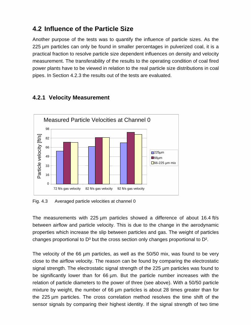
4.2.1 Velocity Measurement

Measured Particle Velocities at Channel 0

0

16

33

49

66

82

98

72 ft/s gas velocity 82 ft/s gas velocity 92 ft/s gas velocity

Par

ticle

vel

ocity

[ft/s

]

225µm 66µm 66-225 µm mix

Fig. 4.3 Averaged particle velocities at channel 0

The measurements with 225 µm particles showed a difference of about 16.4 ft/sbetween airflow and particle velocity. This is due to the change in the aerodynamicproperties which increase the slip between particles and gas. The weight of particleschanges proportional to D³ but the cross section only changes proportional to D².

The velocity of the 66 µm particles, as well as the 50/50 mix, was found to be veryclose to the airflow velocity. The reason can be found by comparing the electrostaticsignal strength. The electrostatic signal strength of the 225 µm particles was found tobe significantly lower than for 66 µm. But the particle number increases with therelation of particle diameters to the power of three (see above). With a 50/50 particlemixture by weight, the number of 66 µm particles is about 28 times greater than forthe 225 µm particles. The cross correlation method resolves the time shift of thesensor signals by comparing their highest identity. If the signal strength of two time

shifts is of the same order, it might be possible to distinguish between the twovelocities. In case of the particle mix the signal strength of the 225 µm particles wasbelow the noise signal level of the 66 µm particles. Therefore, it is obvious that onlythe velocity of the 66 µm particles has been measured. The error in relation to therealistic particle size distribution is estimated in Section 4.2.3.

Velocities of the 225 µm Particles

0

16

33

49

66

82

98

72 ft/s gas velocity 82 ft/s gas velocity 92 ft/s gas velocity

velo

city

[ft/s

]

CH0 CH1 CH2 CH3

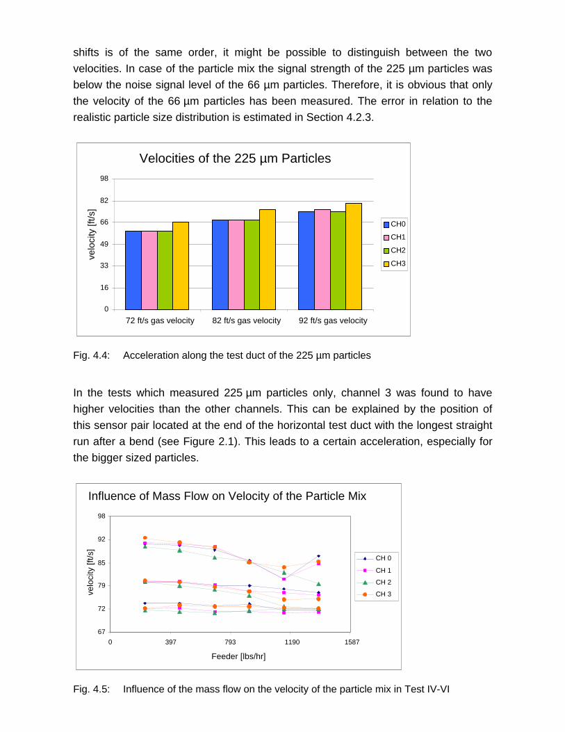
Fig. 4.4: Acceleration along the test duct of the 225 µm particles

In the tests which measured 225 µm particles only, channel 3 was found to havehigher velocities than the other channels. This can be explained by the position ofthis sensor pair located at the end of the horizontal test duct with the longest straightrun after a bend (see Figure 2.1). This leads to a certain acceleration, especially forthe bigger sized particles.

Influence of Mass Flow on Velocity of the Particle Mix

67

72

79

85

92

98

0 397 793 1190 1587

Feeder [lbs/hr]

velo

city

[ft/s

]

CH 0

CH 1

CH 2

CH 3

Fig. 4.5: Influence of the mass flow on the velocity of the particle mix in Test IV-VI

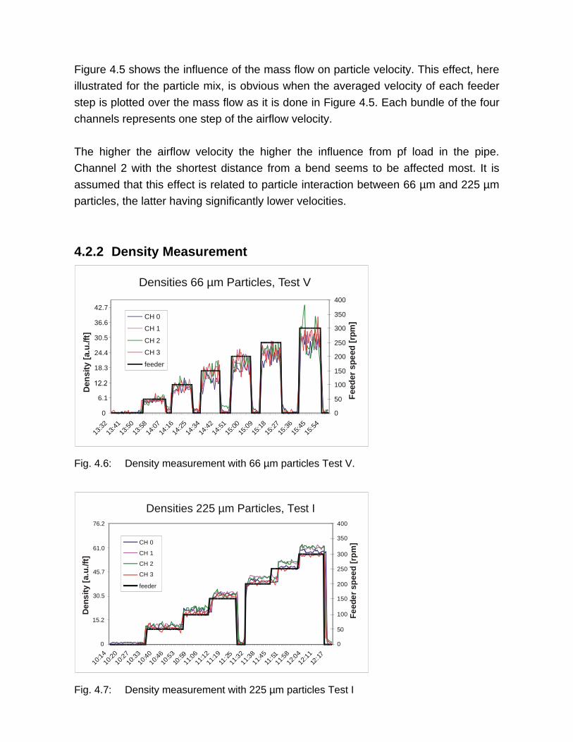
Figure 4.5 shows the influence of the mass flow on particle velocity. This effect, hereillustrated for the particle mix, is obvious when the averaged velocity of each feederstep is plotted over the mass flow as it is done in Figure 4.5. Each bundle of the fourchannels represents one step of the airflow velocity.

The higher the airflow velocity the higher the influence from pf load in the pipe.Channel 2 with the shortest distance from a bend seems to be affected most. It isassumed that this effect is related to particle interaction between 66 µm and 225 µmparticles, the latter having significantly lower velocities.

4.2.2 Density Measurement

Densities 66 µm Particles, Test V

0

6.1

18.3

24.4

30.5

36.6

42.7

13:32

13:4

113

:5013

:58

14:0

714

:1614

:25

14:3

414

:4214

:5115

:0015

:0915

:1815

:2715

:36

15:4

515

:54

0

50

100

150

200

250

300

350

400

CH 0

CH 1

CH 2

CH 3

feeder

Den

sity

[a.u

./ft]

Fee

der

spe

ed [

rpm

]

Fig. 4.6: Density measurement with 66 µm particles Test V.

Densities 225 µm Particles, Test I

0

15.2

30.5

45.7

61.0

76.2

10:14

10:20

10:27

10:3

310

:4010:4

610

:5310

:5911

:0611

:1211

:1911

:2511

:3211:3

811

:4511

:5111

:5812

:0412

:1112

:17

0

50

100

150

200

250

300

350

400

CH 0

CH 1

CH 2

CH 3

feeder

Den

sity

[a.

u./ft

]

Feed

er s

pee

d [r

pm

]

Fig. 4.7: Density measurement with 225 µm particles Test I

The diagrams in Figures 4.6 and 4.7 show the particle size dependent scattering ofthe densities in two test runs. The more extended scattering of the density signal for66 µm particles also increases with the load or particle numbers. With the 225 µmparticles there was less scattering although the densities in Figure 4.7 were nearlytwice as high. The fluctuation quantity for the particle mix is higher than the one forthe 225 µm, but less than the one for the 66 µm particles and was also influenced bythe load (see Figure 3.4).

The scattering of measurement is proved to be realistic and relates to the densityfluctuations of the particle flow. The different behavior can be explained with themean free path between particle collisions. The 66 µm particles have less particle-wall collisions but more particle-particle collisions in a smaller volume. Local highand low density concentrations do not average out within the pipe volume that hasbeen measured.

4.2.3 Mass flow measurement

Influence of the Particle Size

0

500

1000

1500

2000

2500

3000

3500

4000

4500

0 198 397 595 793 992 1190 1389 1587 Feeder mass flow [lb/hr]

Pf-

FLO

mas

s flo

w [

a.u.

/s]

lin average 66 µm lin average 200 µm lin average 66 - 200 µm

2.885

2.734

2.356

Ratio ([a.u.] to [lbs]):

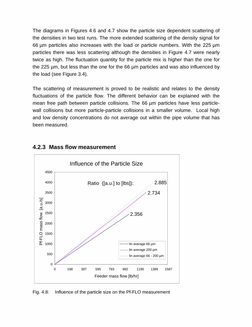
Fig. 4.8: Influence of the particle size on the Pf-FLO measurement

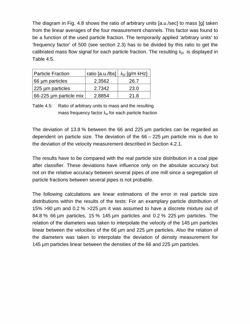
The diagram in Fig. 4.8 shows the ratio of arbitrary units [a.u./sec] to mass [g] takenfrom the linear averages of the four measurement channels. This factor was found tobe a function of the used particle fraction. The temporarily applied ‘arbitrary units’ to‘frequency factor’ of 500 (see section 2.3) has to be divided by this ratio to get thecalibrated mass flow signal for each particle fraction. The resulting kfd is displayed inTable 4.5.

Particle Fraction ratio [a.u./lbs] kfd [g/m kHz]

66 µm particles 2.3562 26.7225 µm particles 2.7342 23.066-225 µm particle mix 2.8854 21.8

Table 4.5: Ratio of arbitrary units to mass and the resulting

mass frequency factor kfd for each particle fraction

The deviation of 13.8 % between the 66 and 225 µm particles can be regarded asdependent on particle size. The deviation of the 66 – 225 µm particle mix is due tothe deviation of the velocity measurement described in Section 4.2.1.

The results have to be compared with the real particle size distribution in a coal pipeafter classifier. These deviations have influence only on the absolute accuracy butnot on the relative accuracy between several pipes of one mill since a segregation ofparticle fractions between several pipes is not probable.

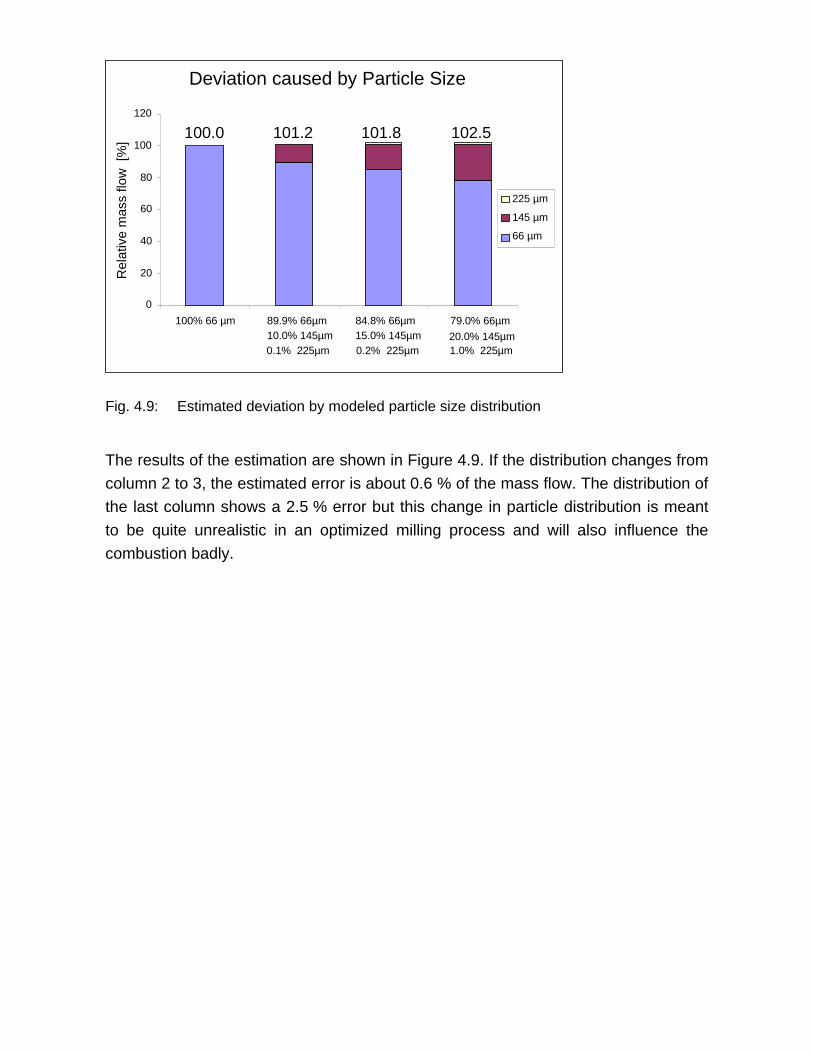
The following calculations are linear estimations of the error in real particle sizedistributions within the results of the tests: For an examplary particle distribution of15% >90 µm and 0.2 % >225 µm it was assumed to have a discrete mixture out of84.8 % 66 µm particles, 15 % 145 µm particles and 0.2 % 225 µm particles. Therelation of the diameters was taken to interpolate the velocity of the 145 µm particleslinear between the velocities of the 66 µm and 225 µm particles. Also the relation ofthe diameters was taken to interpolate the deviation of density measurement for145 µm particles linear between the densities of the 66 and 225 µm particles.

Deviation caused by Particle Size

0

20

40

60

80

100

120

100% 66 µm 89.9% 66µm10.0% 145µm0.1% 225µm

84.8% 66µm15.0% 145µm0.2% 225µm

79.0% 66µm20.0% 145µm1.0% 225µm

Rel

ativ

e m

ass

flow

[%

]

225 µm

145 µm

66 µm

100.0 101.2 101.8 102.5

Fig. 4.9: Estimated deviation by modeled particle size distribution

The results of the estimation are shown in Figure 4.9. If the distribution changes fromcolumn 2 to 3, the estimated error is about 0.6 % of the mass flow. The distribution ofthe last column shows a 2.5 % error but this change in particle distribution is meantto be quite unrealistic in an optimized milling process and will also influence thecombustion badly.

5. Abstract

A reference test at the pneumatic conveying test plant of the “Lehrstuhl fürMechanische Verfahrenstechnik” at the University of Halle-Wittenberg wasestablished to prove the accuracy of a flow measurement system for air-solid flows.The test facility consists of a calibrated screw feeder, a pipe system with vertical andhorizontal elements, and the particle separation equipment. Glass beads were usedas a test medium whose physical properties are comparable to coal dust if taking intoaccount the measurement principle. In addition to the single sized test materials withdiameters of 66 µm and 225 µm, a 50/50 mixture by weight of both particle sizes wasused. The experimental matrix for the tests covered the usual operational range forthe throughput and the velocity in coal pipes of power plants.

In total, four measurement instruments were located at two locations in the upwardrun and two locations in the horizontal run of the test pipe. From the measureddensity and velocity signals of the particles the mass flow was calculated in eachcase and compared with the calibrated feeder signal. The measuring error wasrelated to a single standard deviation.

As a result, the measured deviation from the feeder signal is < 4.5 %; this applies tothe entirety of all four measuring points and all particle fractions. For individualsensors the deviation lies in the range between 1.8 % to 4.3 %, and is in this casenot significantly dependent on the used particle size.

In addition, investigations of the influence of the particle size were carried out. Withinthe wide range of the used particle fractions, the density and velocity measurementshowed some size dependencies. However, the measured differences have only littleinfluence on the accuracy (< 0.6 %) since in utility plants the grading of coal dustusually changes only in a comparable small range.