Embed Size (px)
Citation preview
INAUGURAL-DISSERTATION
zurErlangung der Doktorwurde
an derNaturwissenschaftlich-Mathematischen Gesamtfakultat
der Ruprecht-Karls-Universitat Heidelberg
TANNAKIAN CATEGORIES OF PERVERSE SHEAVES
ON ABELIAN VARIETIES
vorgelegt von
Dipl.-Math. Thomas Kramer
aus Frankenberg (Eder)
Tag der mundlichen Prufung:
Betreuer: Prof. Dr. Rainer Weissauer

Zusammenfassung. Die vorliegende Dissertation beschaftigt sich mitTannaka-Kategorien, welche durch Faltung perverser Garben auf abelschenVarietaten entstehen. Die Konstruktion dieser Kategorien ist eng verbundenmit einem kohomologischen Verschwindungssatz, der ein Analogon zumSatz von Artin-Grothendieck darstellt und als Spezialfall die generischenVerschwindungssatze von Green und Lazarsfeld enthalt. Die erhaltenenTannaka-Gruppen bilden interessante geometrische Invarianten, welche invielen Situationen eine Rolle spielen — nachdem die Grundlagen fur dasStudium dieser Gruppen bereitgestellt sind, wird als ein wichtiges Beispielder Thetadivisor einer prinzipal polarisierten komplexen abelschen Varietatbehandelt. Durch Entartungsargumente wird die Tannaka-Gruppe fur einegenerische abelsche Varietat bestimmt, welche wenigstens in Dimension 4eine neue Antwort auf das Schottky-Problem liefert. Das Faltungsquadratdes Thetadivisors in Dimension 4 hangt eng zusammen mit einer Familieglatter Flachen vom allgemeinen Typ, und ein Studium dieser Familie fuhrtauf eine Variation von Hodge-Strukturen mit Monodromiegruppe W (E6),die mit der Prym-Abbildung verbunden ist. Die Dissertation schließt ab miteiner Rekursionsformel fur den generischen Rang der durch Faltungen vonKurven entstehenden Brill-Noether-Garben auf Jacobischen Varietaten.
Abstract. We study Tannakian categories that arise from convolutions ofperverse sheaves on abelian varieties. The construction of these categoriesis closely intertwined with a cohomological vanishing theorem which is ananalog of the Artin-Grothendieck theorem and contains as a special case thegeneric vanishing theorems of Green and Lazarsfeld. The arising Tannakagroups form a powerful new tool applicable in many different geometriccontexts — after providing the framework for the study of these groups, weconsider as an important example the theta divisor of a complex principallypolarized abelian variety. Using degeneration techniques we determine theassociated Tannaka group for a generic abelian variety, and we show that indimension 4 this yields a Tannakian solution to the Schottky problem. Theconvolution square of the theta divisor in dimension 4 is closely related to afamily of surfaces of general type, and a detailed study of this family leadsto a variation of Hodge structures with monodromy group W (E6) which isconnected with the Prym map. To conclude the dissertation, we provide arecursive formula for the generic rank of Brill-Noether sheaves which arisefrom the convolution of curves on Jacobian varieties.

Acknowledgements
It is a pleasure for me to thank my advisor, Professor R. Weissauer, forsharing his beautiful ideas in many productive mathematical discussions,for his general open-mindedness in all occuring questions, for his carefulreading of the manuscript and for various helpful suggestions concerningthe exposition. I am also grateful to my roommates Johannes Schmidt,Thorsten Heidersdorf and Uwe Weselmann and to the other members of theMathematical Institute at Heidelberg for the pleasant environment whichthey created during the past years. Furthermore I would like to thank severalpeople outside Heidelberg who enlivened the atmosphere on conferencesand expressed their interest in my work, among them Anders Lundman,Bashar Dudin, Christian Schnell, Dan Petersen, Dmitry Zakharov, GiovanniMongardi, Katharina Heinrich, Nicola Tarasca and Paul Hacking. I am alsoindebted to the Studienstiftung des deutschen Volkes and to all membersof its staff for their flexibility and for the financial and ideal support fromwhich I profited a lot. Finally, my most special thanks go to my family andfriends for their encouragement and patience during my work, but perhapseven more for the multifarious, pleasant and interesting distractions from itwithout which I would not have been able to think freely.

Contents
Introduction 1
Some commonly used notations 7
Chapter 1. Vanishing theorems on abelian varieties 91.1. The main result 91.2. A relative generic vanishing theorem 111.3. Kodaira-Nakano-type vanishing theorems 121.4. Negligible perverse sheaves 151.5. The spectrum of a perverse sheaf 17
Chapter 2. Proof of the vanishing theorem(s) 232.1. The setting 232.2. Character twists and convolution 262.3. An axiomatic framework 302.4. The Andre-Kahn quotient 322.5. Super Tannakian categories 352.6. Perverse multiplier 362.7. The main argument 38
Chapter 3. Perverse sheaves on semiabelian varieties 413.1. Vanishing theorems revisited 423.2. Some properties of convolution 463.3. The thick subcategory of negligible objects 473.4. Tannakian categories 513.5. Nearby cycles 543.6. Specialization of characters 583.7. Variation of Tannaka groups in families 61
Chapter 4. The Tannaka group of the theta divisor 694.1. The Schottky problem in genus 4 714.2. Nondegenerate bilinear forms 734.3. Local monodromy 744.4. Degenerations of abelian varieties 794.5. Proof of the main theorem 854.6. Singularities of type Ak 88
v
vi Contents
Chapter 5. A family of surfaces with monodromy W (E6) 935.1. Intersections of theta divisors 955.2. Variations of Hodge structures 1025.3. Integral cohomology 1065.4. Neron-Severi lattices 1095.5. The upper bound W (E6) 1155.6. Negligible constituents 1195.7. Jacobian varieties 1235.8. The difference morphism 1275.9. A smooth global family 131
Chapter 6. The generic rank of Brill-Noether sheaves 1356.1. Brill-Noether sheaves 1356.2. A formula for the generic rank 1376.3. Computations in the symmetric product 1396.4. The fibres of multiple Abel-Jacobi maps 1426.5. Betti polynomials 1446.6. Some numerical values 146
Appendix A. Reductive super groups 151
Appendix B. Irreducible subgroups with bounded determinant 157
Appendix C. An irreducible subgroup of W (E6) 163
Appendix D. Doubly transitive permutation groups 165
Bibliography 169
Introduction
The geometry of a smooth complex projective curve C with Jacobianvariety Jac(C) is governed, after the choice of a base point on the curve, bythe Abel-Jacobi morphism. In particular, the latter defines for each n ∈ Na morphism Cn =C×·· ·×C −→ Jac(C) whose fibres correspond to linearseries of divisors on the curve, and the loci where the fibre dimension jumpsare the subvarieties W r
n ⊆ Jac(C) of special divisors that have been studiedextensively in classical Brill-Noether theory [6].
For smooth complex projective varieties Y of higher dimension one stillhas the Albanese morphism
fn : Y n = Y ×·· ·×Y −→ X = Alb(Y ),
but here the situation is much harder to describe in general. For example, theimage f1(Y ) → X can have any dimension between zero and dim(X), andthere is no obvious substitute for Brill-Noether theory in general. In somesense, the first three chapters of this thesis provide a possible framework forsuch a substitute. More specifically, the properties of fn we are interestedin (such as the loci on X where the fibre dimension jumps) can be studiedvia the higher direct images
Rifn∗(CY n) for i≥ 0,
which are constructible sheaves in the sense that there exists a stratificationof X into finitely many locally closed subvarieties over which they restrictto locally constant sheaves. In general the geometry of these higher directimage sheaves is rather involved, as we will see in a particular example inchapter 5. However, we propose a simple description of such direct imagesin terms of the representation theory of a reductive algebraic group that canbe attached to Y via the Tannakian formalism [33].
The basis for this Tannakian description will be a vanishing theorem forconstructible sheaves on abelian varieties which can be seen as an analogof the Artin-Grothendieck affine vanishing theorem [7, exp. XIV, cor. 3.2]and contains as a special case the generic vanishing theorems of Green andLazarsfeld [47]. For any character χ : π1(X ,0) −→ C∗ of the fundamentalgroup, let us denote by Lχ the corresponding local system on X . Then inchapters 1 and 2 which are based on joint work with R. Weissauer [68],
1
2 Introduction
we show that for any constructible sheaf F on X and a sufficiently generalcharacter χ one has
H i(X ,F⊗C Lχ) = 0 for all i > dim(Supp(F)).
An independent proof of this result has also been given by C. Schnell [94],using the Fourier-Mukai transform for holonomic D-modules. Our proofis of a different flavour and is closely intertwined with the definition of theTannakian categories we are interested in. It is based on an abstract quotientconstruction for semisimple tensor categories — we only use D-modulesat a single place in section 1.4 where we classify all perverse sheaves ofEuler characteristic zero (which will be precisely the objects which becomeisomorphic to zero under the above quotient construction). At present wedo not know whether this classification extends to algebraically closed basefields of positive characteristic p > 0, but otherwise all our arguments alsowork for l-adic constructible sheaves on abelian varieties over the algebraicclosure of a finite field Fp for prime numbers l 6= p.
Our Tannakian results are best formulated in the framework of perversesheaves which has its historic roots in the theory of D-modules [57] andin the sheaf-theoretic construction of intersection cohomology for singularvarieties [10]. Let us for convenience briefly recall some basic definitionsand notations from loc. cit. For any complex algebraic variety Z, we willdenote by Db
c (Z,C) the derived category of bounded C-sheaf complexeswhose cohomology sheaves are constructible for some stratification of Zinto Zariski-locally closed subsets. This is a triangulated category, and onecan define the full abelian subcategory
Perv(Z,C) ⊂ Dbc (Z,C)
of perverse sheaves to be the core of the middle perverse t-structure. Moreexplicitly, a sheaf complex K is said to be semi-perverse if its cohomologysheaves H −i(K) satisfy the support estimate dim(SuppH −i(K)) ≤ i forall i ∈ Z, and it is a perverse sheaf iff both K and its Verdier dual D(K) aresemi-perverse. For example, the perverse intersection cohomology sheaf isby definition the intermediate extension
δZ = j!∗(CU [dim(Z)]) ∈ Perv(Z,C)where j : U → Z denotes the inclusion of a smooth open dense subset. Thisperverse sheaf is self-dual with respect to Verdier duality, and it does notdepend on the choice of the smooth open dense subset. Thus for smoothvarieties Z the perverse intersection cohomology sheaf δZ coincides withthe constant sheaf up to a degree shift. If Z is a closed subvariety of X withembedding i : Z → X , then the direct image i∗ : Perv(Z,C) → Perv(X ,C)is a fully faithful functor, and in this case we will by abuse of notation alsowrite δZ for the perverse sheaf i∗(δZ) ∈ Perv(X ,C).
3
In the context of perverse sheaves, our above vanishing theorem can bereformulated as the statement that for any perverse sheaf P ∈ Perv(X ,C)and a general character χ : π1(X ,0) −→ C∗ the hypercohomology groupssatisfy the property
H i(X ,P⊗C Lχ) = 0 for all i 6= 0,
as we will explain in more detail in chapter 1. Our methods also allowto determine the precise locus S (P) of characters χ for which the abovevanishing property fails. In section 1.5 we will see that this locus is a finiteunion of translates of algebraic subtori of the character torus
Π(X) = Hom(π1(X ,0),C∗),and that for perverse sheaves P ∈ Perv(X ,C) of geometric origin in thesense of [10, sect. 6.2.4] the occuring translations can be taken to be torsionpoints. Again this has been shown independently by C. Schnell in [94] witha different argument. The two approaches seem to be complementary insome sense — for example, whereas in the framework of loc. cit. the proofof the statement about torsion points requires a deep result of C. Simpson,the methods to be explained below allow to reduce it to a statement over afinite field which can be checked directly by looking at the eigenvalues ofthe Frobenius operator, see lemma 1.11.
We now come back to the Albanese morphism fn : Y n −→ X = Alb(Y )of a smooth complex projective variety Y of arbitrary dimension. The grouplaw a : X ×X −→ X of the Albanese variety defines a convolution producton the bounded derived category Db
c (X ,C) by the formula
K ∗M = Ra∗(KM) for K, M ∈ Dbc (X ,C),
and in these terms the direct image of the constant sheaf can be written (upto a degree shift) as the n-fold convolution
R fn∗(δY n) = R f1∗(δY )∗ · · · ∗R f1∗(δY )︸ ︷︷ ︸n times
.
Our goal is to interpret this convolution as a tensor product in the categoryof representations of some reductive algebraic group. To motivate this, letus take a look at the case where Y = C is a curve. Then f1 : C → X is theAbel-Jacobi embedding, and we are interested in the convolution powers ofthe perverse sheaf δC ∈ Perv(X ,C). Although in general these convolutionpowers are not perverse, it turns out that the failure of perversity only comesfrom locally constant sheaves: In view of Gabber’s decomposition theoremwe can write
(δC)∗n = δn ⊕ τn
where τn denotes the maximal direct summand all of whose cohomologysheaves are locally constant on X , and then by [106, th. 7] the remaining
4 Introduction
direct summand δn is a perverse sheaf. Let us say that a perverse sheaf isa Brill-Noether sheaf if it is a subquotient of δn for some n ∈ N. Then fora suitable normalization of the Abel-Jacobi morphism, it has been shownin theorem 14 of loc. cit. that the category of all Brill-Noether sheaves isequivalent to the category of algebraic representations of the group
G(δC) =
Sp2g−2(C) if C is hyperelliptic,Sl2g−2(C) otherwise,
and that the tensor product of representations is induced by the convolutionproduct of perverse sheaves. This Tannakian description reduces classicalgeometric problems to simple computations in representation theory. Forexample, if g denotes the genus of C, then the perverse sheaf δΘ attachedto the theta divisor Θ = Wg−1 ⊂ X corresponds via the above equivalenceto the g− 1st fundamental representation of G(δC). Using this one maydecompose the convolution δΘ ∗ δΘ into its irreducible constituents, whichleads to a new proof of Torelli’s theorem [111].
Alongside our proof of the vanishing theorem and still based on [68], inchapter 2 we generalize the Tannakian constructions from above to the caseof semisimple sheaf complexes on arbitrary complex abelian varieties X . Inparticular, we show that every convolution of semisimple perverse sheavesis a direct sum of a semisimple perverse sheaf and a further sheaf complexwhich is negligible in a suitable sense (for example, on a simple abelianvariety a complex is negligible iff all its cohomology sheaves are locallyconstant). To any semisimple perverse sheaf P ∈ Perv(X ,C) we then attacha reductive algebraic group G(P) whose representation theory governs thedecomposition of the convolution powers P∗n = P∗ · · · ∗P up to negligibledirect summands, see corollary 2.14.
We remark that for algebraic tori in place of abelian varieties, similarresults have been obtained by Gabber and Loeser in [41]. However, in theircase the essential problem is to define the correct notion of convolution inthe non-proper case, and once this has been done, the required propertiesfollow from Artin’s vanishing theorem for affine morphisms. By way ofcontrast, in the case of abelian varieties the main point of the constructionis to find a proper analog of Artin’s theorem, which will be precisely thevanishing theorem that we stated earlier.
The Tannaka groups G(P) attached to perverse sheaves P ∈ Perv(X ,C)as above form an interesting family of new invariants which contain muchinformation about the geometry and the moduli of the underlying abelianvariety. So far the most efficient method to determine such Tannaka groupshas been to study degenerations of the abelian variety (an example for thiscan be found in chapter 4). Even if one is only interested in semisimple
5
perverse sheaves on abelian varieties, such degenerations naturally lead tonon-semisimple perverse sheaves on semiabelian varieties. In chapter 3 weextend our Tannakian constructions to this more general case, combiningthe results of Gabber and Loeser for tori with our vanishing theorem forabelian varieties. We also give a Tannakian description for the functor ofnearby cycles for a family of abelian varieties which degenerates into asemiabelian variety. Even though in the non-proper case the functor ofnearby cycles does not preserve the Euler characteristic, we will show thatthe degenerate Tannaka group is a subgroup of the generic one wheneverone can possibly expect this to hold (see theorem 3.15).
In the remaining chapters we study in more detail the case where P= δΘ
is the perverse intersection cohomology sheaf associated with a symmetrictheta divisor of a principally polarized abelian variety X . In chapter 4 weuse a degeneration argument to show that for a general principally polarizedabelian variety (ppav) of dimension g one has
G(δΘ) =
SOg!(C) if g is odd,Spg!(C) if g is even,
and that δΘ corresponds to the standard representation of this group, a resultthat was conjectured in [67]. As an application we deduce that for g = 4 theinvariant G(δΘ) solves the Schottky problem in the sense that it detects thelocus of Jacobian varieties inside the moduli space A4 of ppav’s.
Once we know the Tannaka group G(δΘ), we can use representationtheory to decompose arbitrary convolution powers of the perverse sheaf δΘ
into their simple constituents. This produces a plethora of interesting simpleperverse sheaves which describe the Hodge theory of various subvarietiesof X . For example, consider the translate Θx = Θ+x of the theta divisor bya point x ∈ X(C). The geometry of the intersections
Yx = Θ∩Θx
is closely connected with the moduli of the underlying ppav and has beenstudied classically in relation with Torelli’s theorem [25], with the Schottkyproblem [27] and with the Prym map [61]. The involution σ = −idX actson these intersections, and if the theta divisor is smooth, then for a generalpoint x ∈ X(C) the quotient variety
Y+x = Yx/σ
will be smooth as well. We will see in chapter 5 that for varying x, thevariable part of the cohomology H•(Y+
x ,Q) can be identified naturally withthe stalk cohomology of the alternating resp. symmetric convolution squareof the perverse sheaf δΘ, depending on whether the dimension g = dim(X)is even or odd. For a general ppav the Tannakian result of chapter 4 implies
6 Introduction
that this alternating resp. symmetric convolution square is irreducible up toa skyscraper sheaf and negligible terms.
So for x varying in a Zariski-open dense subset of X(C), the variablepart of the cohomology of Y+
x defines a variation of Hodge structures whoseunderlying local system is irreducible. The main topic of chapter 5 is a studyof this variation in the case where g = 4. In this case we are dealing witha family of smooth surfaces of general type with a surprisingly explicit andbeautiful geometry. On the level of integral cohomology, we will determinethe Neron-Severi lattices
H2(Yx,Z) and H2(Y+x ,Z)
of the respective surfaces and deduce that the local system underlying theconsidered variation of Hodge structures essentially has the monodromygroup W (E6), see theorem 5.1. We will also see that the appearance of thisWeyl group in the present context is closely related to the ubiquitous 27lines on a cubic surface — the link is provided by the Prym-embeddedcurves on Yx which have been studied by E. Izadi in [61] and appear here asglue vectors for the above Neron-Severi lattices.
In view of this example, it remains an intriguing question to ask for thegeneral relationship between the Tannaka group G(P) attached to a perversesheaf P ∈ Perv(X ,C) and the monodromy groups defined by the simpleperverse sheaves in the corresponding Tannakian category. At present thisrelationship remains mysterious even for Brill-Noether sheaves on Jacobianvarieties. As a first step in this direction, we conclude this dissertation witha recursive formula for the generic rank of Brill-Noether sheaves — in thehope that this formula may be given a representation-theoretic and moreconceptual interpretation at some future time.
Some commonly used notations
Dbc (X ,Λ) derived category of bounded constructible sheaf complexes
on X as defined in [10], in the analytic sense if Λ =C and inthe l-adic sense if Λ is an extension of Ql
Perv(X ,Λ) the abelian subcategory of perverse sheaves in Dbc (X ,Λ)
H i(X ,K) i th hypercohomology group of K ∈ Dbc (X ,Λ)
H ic(X ,K) i th compactly supported hypercohomology group of K
H i(K) i th cohomology sheaf of KpH i(K) i th perverse cohomology sheaf of K
χ(K) Euler characteristic ∑i∈Z(−1)i dimH i(X ,K) of K
Supp(K) support of K
D(K) Verdier dual of K
K(i) i-fold Tate twist of K
δY = ICY [d] perverse intersection cohomology sheaf attached to a closedsubvariety Y → X of dimension d
ΛY constant sheaf with coefficients in the field Λ and support ona closed subvariety Y → X
Π(X) group of all characters χ : π1(X ,0)−→Λ∗ of the topologicalfundamental group, resp. of all continuous characters of thetame etale fundamental group in the l-adic setting
Π(X)l maximal pro-l-subgroup of Π(X)
Lχ local system attached to a character χ ∈Π(X)
Kχ = K⊗Λ Lχ twist of a complex K ∈ Dbc (X ,Λ) by a character χ ∈Π(X)
S (P) spectrum of P ∈ Perv(X ,Λ) as defined in section 1.5
Ψ, Ψ1 functor of nearby cycles resp. its unipotent part
sp specialization functor as defined in section 4.3
G(P) Tannaka group attached to P ∈ Perv(X ,Λ) in corollary 3.10
An, Sn alternating resp. symmetric group of degree n
7

CHAPTER 1
Vanishing theorems on abelian varieties
As we mentioned in the introduction, our construction of Tannakiancategories will be closely intertwined with a vanishing theorem for perversesheaves on abelian varieties. In the first two chapters of this dissertationwhich are based on joint work with R. Weissauer [68], we discuss variousincarnations of this vanishing theorem and explain how it may be proved inan abstract Tannakian framework.
1.1. The main result
Let X be a complex abelian variety. For characters χ : π1(X ,0)−→ C∗of the fundamental group we denote by Lχ the corresponding local systemof complex vector spaces on X of rank one, and for a bounded constructiblesheaf complex K ∈ Db
c (X ,C) we consider the twist Kχ = K⊗C Lχ . Withthese notations, our vanishing theorem can be formulated as
THEOREM 1.1. Let P ∈ Perv(X ,C) be a perverse sheaf. Then for mostcharacters χ we have
H i(X ,Pχ) = 0 for i 6= 0.
Here we use the following terminology: For abelian subvarieties A ⊆ Xlet K(A) be the group of characters χ : π1(X ,0) −→ C∗ whose restrictionto the subgroup π1(A,0)⊆ π1(X ,0) is trivial. We then say that a statementholds for most characters χ if it holds for all χ in the complement of a thinset of characters, where by a thin set of characters we mean a finite unionof translates χi ·K(Ai) for certain non-zero abelian subvarieties Ai ⊆ X andsuitable characters χi of π1(X ,0). The same terminology will be used intheorems 1.4 and 1.5 below for line bundles L ∈ Pic0(X).
The statement of theorem 1.1 can be sharpened as follows. Let Π(X)denote the group of characters χ of the fundamental group π1(X ,0); this isa complex algebraic torus. For a perverse sheaf P ∈ Perv(X ,C) we definethe spectrum
S (P) =
χ ∈Π(X) | H i(X ,Pχ) 6= 0 for some i 6= 0
to be the locus of all characters χ ∈ Π(X) for which the vanishing in theabove theorem fails in some cohomology degree. We will see in section 1.5
9
10 Chapter 1 – Vanishing theorems on abelian varieties
below that the spectrum S (P) is not just contained in a thin subset butactually equal to such a set, in other words
S (P) =n⋃
i=1
χi ·K(Ai)
is a finite union of translates of algebraic subtori K(Ai)⊂ Π(X) for certainabelian subvarieties Ai ⊆ X and χi ∈ Π(X). Furthermore, if the perversesheaf P is of geometric origin in the sense of [10, sect. 6.2.4], we will seethat the characters χi can be chosen to be of finite order.
Our proof of theorem 1.1 is based on two ingredients. The main partis an abstract Tannakian argument to be given in chapter 2 below: Using ageneral construction of Andre and Kahn [1] we show that a certain quotientof the category of semisimple perverse sheaves on X is a rigid symmetricmonoidal semisimple abelian category, and via a criterion by Deligne [30]we deduce that this category is super Tannakian in a sense to be explainedbelow. To see that in the case at hand the construction leads to a Tannakiancategory in the usual sense, we require the second ingredient of the proofwhich is of a more geometric flavour: A classification of perverse sheaveson X with Euler characteristic zero. This classification is independent fromthe Tannakian arguments and uses the theory of D-modules, extending theresults of Franecki and Kapranov [37]. We will discuss it in section 1.4,and this is the only place where we need to work over the base field C. Thearguments of chapter 2 also work for l-adic perverse sheaves on abelianvarieties over the algebraic closure of a finite field.
Our theorem easily generalizes to a relative vanishing theorem for ahomomorphism of abelian varieties as we explain in section 1.2. From adifferent point of view, it can also be reformulated as a statement aboutconstructible sheaves: Indeed, using devissage for the perverse t-structuretogether with Verdier duality one checks that the theorem is equivalent tothe statement that any semi-perverse complex K satisfies H i(X ,Kχ) = 0 forall i > 0 and most characters χ . Note that for any constructible sheaf F thedegree shift K = F [dim(SuppF)] is a semi-perverse sheaf complex, so wein particular obtain
THEOREM 1.2. Let F be a constructible sheaf on X. Then for mostcharacters χ we have
H i(X ,Fχ) = 0 for i > dim(SuppF).
This can be viewed as an analog of the Artin-Grothendieck affine vanishingtheorem in the same way as one can consider the generic vanishing theoremof Green and Lazarsfeld [47, th. 1] as an analog of the Kodaira-Nakanovanishing theorem. Motivated by this observation, in section 1.3 we explain
1.2. A relative generic vanishing theorem 11
how to recover a stronger version of the Green-Lazarsfeld theorem as aspecial case of our result. In the remaining sections of this chapter wethen discuss perverse sheaves with Euler characteristic zero and, as a firstapplication, deduce from the obtained classification the statement about thespectrum of a perverse sheaf mentioned above.
1.2. A relative generic vanishing theorem
Let A⊆ X be an abelian subvariety and f : X −→ B = X/A the quotientmorphism. Assuming theorem 1.1 only for the abelian variety A, we obtainthe following relative generic vanishing theorem. We remark that here thequantifier most can be read in the slightly stronger sense that it does notrefer to the characters of π1(X ,0) but only to their pull-back to π1(A,0) aswe will explain in more detail at the end of section 1.5 below.
THEOREM 1.3. Let P ∈ Perv(X ,C). Then for most characters χ thedirect image R f∗(Pχ) is a perverse sheaf on B.
Proof. By Verdier duality it will be enough to show that for most χ thedirect image complex R f∗(Pχ) satisfies the semi-perversity condition
dim(Supp H −k(R f∗(Pχ))
)≤ k for all k ∈ Z.
To check this condition, note that by lemma 2.4 and section 3.1 in [12] wecan find Whitney stratifications X = tβ Xβ and B = tαBα such that thefollowing properties hold:
(a) for all β , i, χ the cohomology sheaves H −i(Pχ) =H −i(P)⊗CLχ
are locally constant on the strata Xβ ,(b) each f (Xβ ) is contained in some Bα ,(c) for all α,β with f (Xβ )⊆Bα the morphism f : Xβ →Bα is smooth.
By theorem 4.1 of loc. cit. then the restriction H −k(R f∗(Pχ))|Bαis locally
constant for all α , k and χ . Now there are only finitely many strata Bα ,and we have H −k(R f∗(Pχ)) 6= 0 for only finitely many k. Hence it followsthat if the direct image complex R f∗(Pχ) were not semi-perverse for mostcharacters χ , then we could find α and k such that
(d) dim(Bα) > k (where as usual by the dimension of a constructiblesubset we mean the maximum of the dimensions of the irreduciblecomponents of its closure), and
(e) H −k(R f∗(Pχ))b 6= 0 for all points b ∈ Bα(C) and all χ in a setof characters which is not thin in the sense of the introduction.
Indeed, if a property does not hold for most characters, then by definition itfails on a set of characters which is not thin. Fixing α and k as above, wenow argue by contradiction.
12 Chapter 1 – Vanishing theorems on abelian varieties
Choose a point b ∈ Bα(C). Consider the fibre Fb = f−1(b), and forany character χ denote by Mb = Pχ |Fb the restriction of Pχ to Fb (in whatfollows we suppress the character twist in this notation). For the perversecohomology sheaves
Mrb = pH−r(Mb)
we have the spectral sequence
Ers2 = H−s(Fb,Mr
b) =⇒ H−(r+s)(Fb,Mb) = H −(r+s)(R f∗(Pχ))b.
Theorem 1.1 for Fb∼= A shows that for most χ we have H−s(Fb,Mr
b) = 0 forall s 6= 0 and all r ∈ Z. For such χ the spectral sequence degenerates, i.e.
H −k(R f∗(Pχ))b = H0(Fb,Mkb).
On the other hand, by (e) we can assume H −k(R f∗Pχ)b 6= 0. By the abovethen Mk
b 6= 0. Since Mkb = pH0(Mb[−k]), it follows by definition of the
perverse t-structure that
dim(Supp H −i(Mb)
)= i− k ≥ 0 for some i ∈ Z.
Now by (a) the support of H −i(Pχ) is a union of certain strata Xβ , so usingthe above dimension estimate and the definition of Mb = Pχ |Fb we find astratum Xβ ⊆ Supp H −i(Pχ) with dim(Fb∩Xβ ) = i− k. Since by (b), (c)the stratum Xβ is equidimensional over Bα , it follows that
dim(Supp H −i(Pχ)
)≥ dim(Xβ ) = i− k+dim(Bα).
But dim(Bα)> k by property (d), so it follows that the perverse sheaf Pχ isnot semi-perverse, a contradiction.
Note that in the proof of theorem 1.3 we have only used theorem 1.1 forthe fibres f−1(b) ∼= A but not for X itself. Indeed, using this observationand assuming theorem 1.1 only for simple abelian varieties, one can byinduction on the dimension deduce for arbitrary abelian varieties a slightlyweaker version of theorem 1.1 where most is replaced by generic [107].
1.3. Kodaira-Nakano-type vanishing theorems
From theorem 1.1 one easily recovers stronger versions of the genericvanishing theorems of Green and Lazarsfeld as follows. Let Y be a compactconnected Kahler manifold of dimension d whose Albanese variety Alb(Y )is algebraic, and denote by
f : Y −→ X = Alb(Y )
the Albanese morphism. To pass from coherent to constructible sheaves,recall that every line bundle L ∈ Pic0(X) admits a flat connection; thehorizontal sections with respect to such a connection form a local systemcorresponding to a character χ ∈Π(X) such that L ∼= Lχ ⊗C OX .
1.3. Kodaira-Nakano-type vanishing theorems 13
For a given line bundle L ∈ Pic0(X), the set of all characters χ with theabove property is a torsor under the group H0(X ,Ω1
X). Indeed, this followsfrom the truncated exact cohomology sequence
0 −→ H0(X ,Ω1X) −→ H1(X ,C∗) −→ Pic0(X) −→ 0
attached to the exact sequence 0→ C∗X → O∗X → Ω1X ,cl → 0 where Ω1
X ,cldenotes the sheaf of closed holomorphic 1-forms. On the other hand, fromthe point of view of Hodge theory it is better to restrict our attention tounitary characters χ : π1(X ,0)→U(1) = z ∈ C∗ | |z|= 1, which has theextra benefit of making the passage from coherent to constructible sheavesunique: Comparing the exponential sequences 0→ZX→RX→U(1)X→ 0and 0→ ZX → OX → O∗X → 0 one sees that the morphism
H1(X ,U(1))∼=−→ Pic0(X)
is an isomorphism, so for every line bundle L ∈ Pic0(X) there is a uniqueunitary character χ with L ∼= Lχ ⊗C OX . Concerning the applicability oftheorem 3.1 in this unitary context, we remark that the intersection of anythin subset of Π(X) with the set of unitary characters is mapped via theabove isomorphism to a thin subset of Pic0(X).
In what follows, for n ∈N0 we put Xn = x ∈ X | dim( f−1(x)) = n andconsider the number
w(Y ) = min
2d− (dim(Xn)+2n) | n ∈ N0, Xn 6=∅.
Notice that w(Y ) ≤ d (indeed, for some n the preimage f−1(Xn) is densein Y so that d = dim( f−1(Xn)) = dim(Xn)+n, hence 2d− (dim(Xn)+2n)is equal to 2d− (d + n) = d− n ≤ d). Furthermore, by base change onechecks that for any local systems E of complex vector spaces on Y thedirect image
R f∗E[2d−w(Y )] is semi-perverse,
because for x ∈ Xn(C) the fibre F = f−1(x)⊆Y satisfies H i(F,E|F) = 0 forall i > 2n. This being said, theorem 1.1 implies the following version of thevanishing theorem given in [47, th. 2].
THEOREM 1.4. Let E be a unitary local system on Y . Then for most Lin Pic0(Y ) we have
H p(Y,ΩqY (E⊗C L )) = 0 if p+q < w(Y ).
Proof. The morphism f ∗ : Pic0(X) −→ Pic0(Y ) is an isomorphism byconstruction of the Albanese variety [48, p. 553], so every coherent linebundle L ∈ Pic0(Y ) arises as the pull-back of some M ∈ Pic0(X). Asexplained above, there is a unitary character χ such that
M ∼= OX ⊗C Lχ .
14 Chapter 1 – Vanishing theorems on abelian varieties
Then L ∼= f ∗(M ) ∼= OY ⊗C f ∗(Lχ). Since all the occuring local systemsare unitary, Hodge theory says that⊕
p+q=k
H p(Y,ΩqY (E⊗C L )) ∼= Hk(Y,E⊗C f ∗(Lχ)).
Putting K = R f∗E[2d−w(Y )] we can identify the cohomology group on theright hand side with the group Hk−2d+w(Y )(X ,Kχ). Since the direct imagecomplex Kχ is semi-perverse, theorem 1.1 shows that for k > 2d−w(Y )and most characters χ the above group vanishes. The theorem now followsby an application of Serre duality.
For a similar result in this direction, consider for n ∈ N0 the closedanalytic subsets
Xn = x ∈ X | dim( f−1(x))≥ n and Y n = f−1(Xn),
and put dn = dim(Y n) with the convention that dn = −∞ for Y n = /0. Thenour vanishing theorem implies the following
THEOREM 1.5. Suppose that p+ q = d− n for some n ≥ 1. Then formost line bundles L ∈ Pic0(Y ),
H p(Y,ΩqY (L )) = 0 unless d−dn ≤ p,q ≤ dn−n.
Proof. By Serre duality the claim is equivalent to the statement thatif p+q = d+n for some n≥ 1, then H p(Y,Ωq
Y (L )) = 0 for most L unlessthe Hodge types satisfy the estimates
d +n−dn ≤ p,q ≤ dn.
In fact it will suffice to establish the upper estimate p,q ≤ dn, the lowerestimate is then automatic since p+q = d +n by assumption.
The decomposition theorem for compact Kahler manifolds [90, th. 0.6]says that R f∗CY [d]∼=
⊕m Mm[−m] where each Mm is a pure Hodge module
on X of weight m+ d in the sense of [89]. Furthermore, for any unitarycharacter χ with complex conjugate χ the local system Lχ⊕Lχ of rank twohas an underlying real structure and hence can be viewed as a real Hodgemodule of weight zero in a natural way. So for any real Hodge module Mon X also Mχ,χ = Mχ ⊕Mχ is a real Hodge module. This being said, bytheorem 1.1 we have
Hd+n(Y, f ∗(Lχ ⊕Lχ)) ∼= Hn(X ,(R f∗CY [d])χ,χ) ∼= H0(X ,(Mn)χ,χ)
for most unitary characters χ . The formalism of Hodge modules equips thecohomology group on the right hand side with a pure R-Hodge structure ofweight n+d compatible with the natural one on the left hand side. We arelooking for bounds on the types (p,q) in this Hodge structure.
1.4. Negligible perverse sheaves 15
One easily checks that Supp(Mn)⊆ Xn, so Mn[−n] is a direct summandof R f∗CYn
[d] by base change. To control the Hodge structure on twists ofthe cohomology of this direct image, let π : Y → Y be a composition ofblow-ups in smooth centers that gives rise to an embedded resolution ofsingularities Yn = π−1(Y n)→ Y n, see [56] or [11, th. 10.7]. Then CY [d]occurs as a direct summand of the complex Rπ∗CY [d] by the decompositiontheorem, so the restriction CY n
[d] is a direct summand of Rπ∗CYn[d]. It then
follows that Mn[−n] is a direct summand of R f∗Rπ∗CYn[d], and we get an
embedding
H0(X ,(Mn)χ,χ) → Hd+n(Yn,π∗ f ∗(Lχ ⊕Lχ−1)).
But the Hodge types (p,q) on the right hand side satisfy p,q≤ dim(Yn)= dnas one may check from the Hodge theory of compact Kahler manifolds withcoefficients in unitary local systems.
The above result contains the generic vanishing theorem of Green andLazarsfeld [47, second part of th. 1] as the special case q = 0. Indeed, forany p < dim( f (Y )) the number n = d− p is larger than the dimension of thegeneric fibre of the Albanese morphism, hence dn < d so that H p(Y,L ) = 0for most L by theorem 1.5. If Y is algebraic, the theorem also holds moregenerally for H p(Y,Ωq
Y (E⊗C L )) with a unitary local system E on Y .
In general the bounds in the above theorem are strict: If d = 4 and if Yis the blow-up of X along a smooth algebraic curve C ⊂ X of genus ≥ 2,then one has w(Y ) = d1 = 3 but H2(Y,Ω1
Y (L )) 6= 0 for all non-trivial linebundles L as explained in [47, top of p. 402].
1.4. Negligible perverse sheaves
A crucial ingredient for the proof of our vanishing theorem to be givenin section 2.7 will be a classification of all perverse sheaves on X of Eulercharacteristic zero. To obtain this classification we use an index formula forD-modules, extending the arguments of [37, cor. 1.4] which have shownthat on a complex abelian variety X every perverse sheaf P ∈ Perv(X ,C)has Euler characteristic χ(P)≥ 0. As we mentioned earlier, this is the onlypart of our proof of theorem 1.1 which so far only works over C.
PROPOSITION 1.6. Let P ∈ Perv(X ,C) be a simple perverse sheaf.(a) One has χ(P) = 0 iff there exists an abelian subvariety A → X of
positive dimension with quotient morphism q : X B = X/A suchthat
P ∼= Lϕ ⊗q∗(Q)[dim(A)]for some Q ∈ Perv(B,C) and some character ϕ ∈Π(X).
(b) One has χ(P) = 1 iff P is a skyscraper sheaf on X of rank one.
16 Chapter 1 – Vanishing theorems on abelian varieties
Proof. Via the Riemann-Hilbert correspondence [57] we can consider Pas a D-module. For Z ⊆ X closed and irreducible, let ΛZ ⊆ T ∗X be theclosure in T ∗X of the conormal bundle in X to the smooth locus of Z. As inloc. cit. we write the characteristic cycle of P as a finite formal sum
CC(P) = ∑Z⊆X
nZ ·ΛZ with nZ ∈ N0,
where Z runs through all closed irreducible subsets of X . From CC(P) thesupport of P can be recovered via SuppP =
⋃nZ 6=0 Z. Furthermore, by the
microlocal index formula [44, th. 9.1] we have
χ(P) = ∑Z⊆X
nZ ·dZ with dZ = [ΛX ] · [ΛZ] ∈ Z.
The intersection numbers dZ are well-defined even though ΛZ is not properfor Z 6= X , see loc. cit. for details. Now if X is a simple abelian variety, thenlemma 1.8 below implies (a), and if we additionally assume dim(X) > 1,also (b) follows in view of lemma 1.9 below. The non-simple case can bereduced to the simple case, see [107].
The reduction to the case of simple abelian varieties in loc. cit. works forground fields k of characteristic p > 0 as well, but we do not know how todeal with simple abelian varieties in that case. For k =C, Christian Schnellhas given in [94, cor. 3.11] a different proof of proposition 1.6(a) via theFourier-Mukai transform for D-modules.
COROLLARY 1.7. A simple perverse sheaf P ∈ Perv(X ,C) has Eulercharacteristic zero iff H•(X ,Pχ) = 0 for most characters χ .
Proof. “⇐” holds by corollary 2.2. For “⇒” take a positive-dimensionalabelian subvariety A → X with quotient q : X B = X/A and a character ϕ
such that P ∼= Lϕ ⊗ q∗(Q)[dim(A)] for some perverse sheaf Q on B as inproposition 1.6(a). We can assume that the Euler characteristic of Q is notzero. Then we claim that
H•(X ,Pχ) = H•(B,Rq∗(Pχ)) = H•(B,Rq∗(Lϕχ)⊗Q[dim(A)])
vanishes iff the restriction of the local system Lϕχ to A = ker(q) ⊆ X isnot trivial. Indeed, if this restriction is non-trivial, then by base change onechecks that Rq∗(Lϕχ) = 0 and hence a fortiori H•(X ,Pχ) = 0. On the otherhand, if this restriction is trivial, then Lϕχ = q∗(Lψ) for some character ψ
and then H•(X ,Pχ) = H•(A,C)⊗H•(B,Qψ)[dim(A)] is non-zero since theEuler characteristic of Qψ is not zero.
For completeness we include the following two elementary lemmasabout characteristic cycles that have been used, in the case of simple abelianvarieties, in the proof of proposition 1.6.
1.5. The spectrum of a perverse sheaf 17
LEMMA 1.8. With notations as above, dZ ≥ 0 for all Z. One has dZ = 1iff Z is reduced to a single point. If X is simple, then dZ = 0 iff Z = X.
Proof. Put g = dim(X). The cotangent bundle T ∗X = X ×Cg is trivial,and projecting from ΛZ ⊆ T ∗X onto the second factor Cg induces the Gaußmapping p : ΛZ → Cg. By [37, prop. 2.2] the intersection number dZ is thegeneric degree of p. In particular dZ ≥ 0 for all Z.
If dZ = 1, then ΛZ is birational to Cg, so by [75, cor. 3.9] there does notexist a non-constant map from ΛZ to an abelian variety. So the image Z ofthe composite map ΛZ ⊆ T ∗X −→ X consists of a single point.
If dZ = 0, then p is not surjective, so dim(p(ΛZ)) < g. Then for somecotangent vector ω ∈ p(ΛZ) the fibre p−1(ω) is positive-dimensional, andfor Z 6= X we can assume ω 6= 0. Let Y ⊆ X be the image of p−1(ω)⊆ T ∗Xunder the map T ∗X −→ X . Then dim(Y )> 0, and up to a translation we canassume 0∈Y . By construction ω is normal to Y in every smooth point of Y ,so the preimage of Y under the universal covering Cg −→ X =Cg/Λ lies inthe hyperplane of Cg orthogonal to ω . Accordingly the abelian subvarietyof X generated by Y is strictly contained in X , but not zero. This contradictsour assumption that X is simple.
LEMMA 1.9. Put g = dim(X), and assume P ∈ Perv(X ,C) is simple. Ifthere is a closed subset Y ⊂ X with dim(Y )≤ g−2 such that
CC(P) = nX ΛX + ∑Z⊆Y
nZΛZ and nX > 0,
then P = Lχ [g] for some character χ , hence nX = 1 and nZ = 0 for Z 6= X.
Proof. Consider the open embedding j : U = X \Y → X . Since openembeddings are non-characteristic for any DX -module, by [57, sect. 2.4]we have CC( j∗(P)) = CC(P)∩T ∗U = nX ·ΛU . So we get j∗(P) = LU [g]for a local system LU on U by prop. 2.2.5 in loc. cit. Since X is smooth,the purity of the branch locus and dim(Y )≤ g−2 implies LU = j∗(L) for alocal system L on X . By simplicity of P it follows that P = L[g], and as anirreducible representation of the abelian group π1(X ,0) the local system Lmust have rank one.
1.5. The spectrum of a perverse sheaf
Using the classification from the previous section, we now explain howto determine for P ∈ Perv(X ,C) the spectrum
S (P) =
χ ∈Π(X) | H i(X ,Pχ) 6= 0 for some i 6= 0.
As a refinement of theorem 1.1 we will show that S (P) is a finite union oftranslates of proper algebraic subtori of Π(X) and that furthermore for P of
18 Chapter 1 – Vanishing theorems on abelian varieties
geometric origin each of the occuring translations can be taken to be torsionpoints of Π(X), see lemma 1.11 below. More generally, for semisimplesheaf complexes K =
⊕n∈Z
pH−n(K)[n] we define
S (K) =⋃
n∈ZS (pH−n(K)).
The definitions imply that S (Kχ) = χ−1 ·S (K) for all χ ∈Π(X), and forall semisimple K1,K2 we have
S (K1 ∗K2) ⊆ S (K1)∪S (K2) = S (K1⊕K2),
where K1∗K2 denotes the convolution of K1 and K2 as defined in section 2.1below. Note that the equality displayed on the right hand side reduces thecomputation of the spectrum of semisimple sheaf complexes to the caseof simple perverse sheaves. Of course the spectrum S (P) may be empty,for example if P is a skyscraper sheaf or, more interestingly, if P = i∗E[1]where i : C → X is the embedding of a smooth curve in X and where E isan irreducible local system on C of rank at least two.
Since π1(X ,0) ∼= Z2g, the character group Π(X) ∼= C2g is a complexalgebraic torus of rank 2g. Furthermore Π is a contravariant functor: Forany homomorphism h : X −→ B of complex abelian varieties, the pull-backof characters gives rise to a homomorphism Π(h) : Π(B)−→Π(X) betweenthe corresponding algebraic tori.
REMARK 1.10. The functor Π has the following properties.
(a) Let h : X → B be an isogeny with kernel F. Then we have an exactsequence
0 // Hom(F,C∗) // Π(B)Π(h)
// Π(X) // 0.
For P∈ Perv(X ,C) we have h∗(P)∈ Perv(B,C), and Π(h) inducesa surjection
S (h∗(P))S (P).
(b) Let i : A → X be an embedding of abelian varieties with quotientmorphism q : X → B = X/A. Then we have an exact sequence
0 // Π(B)Π(q)
// Π(X)Π(i)
// Π(A) // 0.
In this situation we denote by K(A)⊆Π(X) the image of Π(q).
Proof. The exactness of the considered sequences can be seen from thedescription of a complex abelian variety as the quotient of a complex vectorspace modulo a lattice. For the surjectivity S (g∗(P))S (P) in part (a)one can use that H i(X ,Pϕ) = H i(B,g∗(P)χ) for the pull-back ϕ = Π(g)(χ)and that Π(g) is surjective.
1.5. The spectrum of a perverse sheaf 19
In what follows, let E(X) be the class of all semisimple perverse sheaveson X with Euler characteristic zero. We say that a perverse sheaf is cleanif it does not contain constituents from E(X). For x ∈ X(C) we denoteby tx : X→ X the translation morphism y 7→ x+y, and for K ∈Db
c (X ,C) weconsider the stabilizer
Stab(K) = x ∈ X(C) | t∗x (K)∼= K.
By constructibility of K this is an algebraic subset of X , and its connectedcomponent Stab(K)0 ⊆ Stab(K) is an abelian subvariety of X . We can nowformulate the main result of the present section.
LEMMA 1.11. (a) Let P∈E(X) be a semisimple perverse sheaf of Eulercharacteristic zero. Then a character χ lies in S (P) iff H•(X ,Pχ) 6= 0. Inparticular, if P is simple, there exists a character ϕ such that
S (P) = ϕ−1 ·K(A) for A = Stab(P)0
where K(A)⊂Π(X) is the algebraic subtorus from remark 1.10(b).
(b) For any semisimple perverse sheaf P on X there are non-zero abeliansubvarieties A1, . . . ,An ⊆ X and χ1, . . . ,χn ∈Π(X) such that
S (P) =n⋃
i=1
χi ·K(Ai).
(c) If in part (b) the semisimple perverse sheaf P is of geometric origin inthe sense of [10, 6.2.4], then the χi can be chosen to be torsion characters.
Proof. (a) The first statement is obvious from proposition 1.6(a), andthe second one follows easily from the proof of corollary 1.7.
(b) The proof of this part is most conveniently formulated in terms of theconvolution product ∗ to be defined in section 2.1 below. For the time beingit suffices to know that the convolution of semisimple sheaf complexes isagain a semisimple sheaf complex by Gabber’s decomposition theorem, thatfor K,M ∈ Db
c (X ,C) we have the Kunneth formula
H•(X ,K ∗M) = H•(X ,K)⊗C H•(X ,M)
and that convolution is compatible with character twists in the sense that forall χ ∈Π(X) we have (K ∗M)χ
∼= Kχ ∗Mχ , see proposition 2.1. Hence forthe g-fold convolution power of a semisimple perverse sheaf P∈ Perv(X ,C)it follows from theorem 1.1 that P∗g = Q⊕
⊕ν∈ZNν [ν ] where Q is a clean
semisimple perverse sheaf and the Nν are semisimple perverse sheavesin E(X). So for any χ ∈Π(X) we obtain
(?) H•(X ,Pχ)⊗g = H•(X ,Qχ) ⊕
⊕ν∈Z
H•(X ,(Nν)χ)[ν ].
20 Chapter 1 – Vanishing theorems on abelian varieties
If χ ∈S (P), then H•(X ,Pχ) is not concentrated in degree zero, so (?) isnon-zero in some degree d with |d| ≥ g. But Q is a clean perverse sheaf andas such it does not contain the constant perverse sheaf, hence
Hd(X ,Qχ) = 0 for |d| ≥ g
by the adjunction property in [10, prop. 4.2.5]. So it follows from the abovethat H•(X ,(Nν)χ) 6= 0 for some index ν and hence that χ ∈ S (Nν) bypart (a). Conversely, χ ∈ S (Nν) implies by proposition 1.6(a) that thehypercohomology H•(X ,(Nν)χ) is non-zero in more than one cohomologydegree; then by (?) the same holds for H•(X ,Pχ), so χ ∈S (P). Altogetherthis shows
S (P) =⋃
ν∈ZS (Nν),
and part (b) of our claim follows by applying part (a) to the Nν ∈ E(X).
(c) First we claim that a local system Lχ is of geometric origin iff χ
is a torsion character. For the non-trivial direction note that if Lχ is ofgeometric origin, then X has a model XA over a subring A⊂C of finite typeover Z such that Lχ descends to a local system on XA, corresponding to acontinuous character
χA : π1(XA) −→ Q∗l .
Take a closed point of Spec(A) with finite residue field κ . Let V ⊂ C bea strictly Henselian ring with A ⊂ V whose residue field is an algebraicclosure κ of κ . For XV = XA×A V the inclusion of the special fibre Xκ
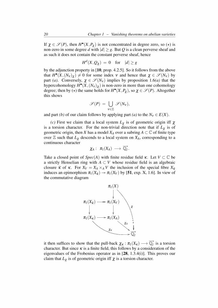
induces an epimorphism π1(Xκ) π1(XV ) by [51, exp. X, 1.6]. In view ofthe commutative diagram
π1(X)
χ
π1(Xκ) // //
π1(XV )
π1(Xκ) //
χκ
11
π1(XA)χA
""FFF
FFFF
FF
Q∗l
it then suffices to show that the pull-back χκ : π1(Xκ) −→ Q∗l is a torsioncharacter. But since κ is a finite field, this follows by a consideration of theeigenvalues of the Frobenius operator as in [28, 1.3.4(i)]. This proves ourclaim that Lχ is of geometric origin iff χ is a torsion character.
1.5. The spectrum of a perverse sheaf 21
Now for P of geometric origin the perverse sheaves Nν ∈ E(X) in (b)and hence also all their simple constituents N are of geometric origin. Eachsuch constituent has the form N ∼= Lϕ ⊗ q∗(Q)[dim(A)] for suitable ϕ andsome abelian subvariety A ⊆ X as in proposition 1.6(a). In this situationthe pullback i∗(N) to A is an isotypic multiple of i∗(Lϕ) and of geometricorigin. Hence Π(i)(ϕ) is a torsion character. Writing S (N) = χ ·K(A) wecan take for χ−1 any torsion character in Π(i)−1(Π(i)(ϕ)).
The above arguments can also be generalized to the relative setting oftheorem 1.3. For a homomorphism f : X → B of abelian varieties, definethe relative spectrum S f (P) of a perverse sheaf P ∈ Perv(X ,C) to be theset of all χ ∈Π(X) such that R f∗(Pχ) is not perverse. By abuse of notation,for χ ∈ Π(X) and ψ ∈ Π(B) we write χψ = χ · (Π( f )(ψ)) ∈ Π(X). Thenthe projection formula shows
R f∗(Pχψ) = (R f∗(Pχ))ψ ,
hence S f (P) is invariant under Π(B). In particular, if B = X/A for anabelian subvariety A ⊆ X , then S f (P) is determined by its image S f (P)in Π(A) = Π(X)/Π(B). Furthermore, in the situation of theorem 1.3 theassertion for most characters can be read in Π(A), i.e. in the stronger sensethat S f (P) is contained in a finite union of translates of proper algebraicsubtori of Π(A). Indeed we have
LEMMA 1.12. S f (P)⊆S (P) ·Π(B).
Proof. If a character χ is not in S (P) ·Π(B), then for any ψ ∈ Π(B)we have χψ /∈S (P) and hence Hn(X ,Pχψ) = Hn(B,(R f∗(Pχ))ψ) 6= 0 forsome n 6= 0. By theorem 1.1 then R f∗(Pχ) is not perverse.

CHAPTER 2
Proof of the vanishing theorem(s)
In this chapter we give an abstract Tannakian proof of theorem 1.1 basedon joint work with R. Weissauer [68]. As a geometric input we only requirethe classification of perverse sheaves with Euler characteristic zero fromsection 1.4. For this classification we have used the theory of D-modules,and at present we do not know whether it also holds over a ground fieldof positive characteristic. However, since this is the only reason why forthe time being the proof only applies to complex abelian varietes, in whatfollows we formulate our arguments in a uniform way including also thecase of l-adic perverse sheaves in positive characteristic.
2.1. The setting
Let X be an abelian variety over an algebraically closed field k whichhas characteristic zero or is the algebraic closure of a finite field. As in [10]we consider the derived category Db
c (X ,Λ) of complexes of Λ-sheaves withbounded constructible cohomology sheaves, where Λ is either a subfieldof Ql for some fixed prime number l 6= char(k) or a subfield of C if we areworking over the base field k = C. We denote by Perv(X ,Λ) ⊂ Db
c (X ,Λ)the full abelian subcategory of perverse sheaves as defined in loc. cit., andwe write π1(X ,0) for the etale fundamental group, resp. for the topologicalfundamental group in the complex case. By a character χ : π1(X ,0)−→ Λ∗
we mean in the etale setting a continuous character with image in a finiteextension field of Ql . Any such character defines a local system Lχ , and asin the previous chapter we denote by Kχ = K⊗Λ Lχ the corresponding twistof a complex K ∈ Db
c (X ,Λ).
Our Tannakian proof of theorem 1.1 relies on the notion of convolutionof sheaf complexes. Let a : X×X −→ X denote the group law, and considerthe convolution product
∗ : Dbc (X ,Λ)×Db
c (X ,Λ) −→ Dbc (X ,Λ), K1 ∗K2 = Ra∗(K1K2).
It has been shown in [106, sect. 2.1] that the category Dbc (X ,Λ) equipped
with this convolution product is a symmetric monoidal category in the senseof [73, sect. VII.7]. In other words, there exists a unit object 1 in Db
c (X ,Λ)
23
24 Chapter 2 – Proof of the vanishing theorem(s)
such that we have natural unity constraints
K ∗1∼=←− K
∼=−→ 1∗K
and natural commutativity and associativity constraints
SK,L : K ∗L∼=−→ L∗K and AK,L,M : K ∗ (L∗M)
∼=−→ (K ∗L)∗M
for all objects K,L,M in Dbc (X ,Λ), and these constraints satisfy the usual
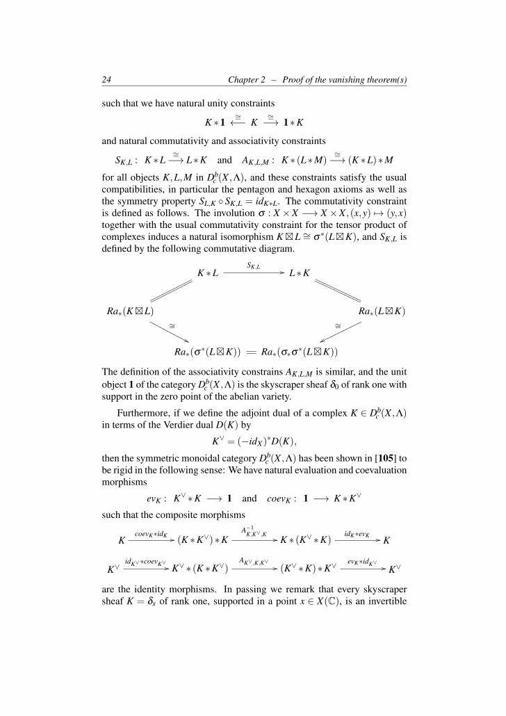
compatibilities, in particular the pentagon and hexagon axioms as well asthe symmetry property SL,K SK,L = idK∗L. The commutativity constraintis defined as follows. The involution σ : X ×X −→ X ×X ,(x,y) 7→ (y,x)together with the usual commutativity constraint for the tensor product ofcomplexes induces a natural isomorphism KL ∼= σ∗(LK), and SK,L isdefined by the following commutative diagram.
K ∗LSK,L //
ooooooooooo
oooooooooooL∗K
PPPPPPPPPPPP
PPPPPPPPPPPP
Ra∗(KL)∼=
''NNNNNNNNNNNRa∗(LK)
∼=
wwooooooooooo
Ra∗(σ∗(LK)) Ra∗(σ∗σ∗(LK))
The definition of the associativity constrains AK,L,M is similar, and the unitobject 1 of the category Db
c (X ,Λ) is the skyscraper sheaf δ0 of rank one withsupport in the zero point of the abelian variety.
Furthermore, if we define the adjoint dual of a complex K ∈ Dbc (X ,Λ)
in terms of the Verdier dual D(K) by
K∨ = (−idX)∗D(K),
then the symmetric monoidal category Dbc (X ,Λ) has been shown in [105] to
be rigid in the following sense: We have natural evaluation and coevaluationmorphisms
evK : K∨ ∗K −→ 1 and coevK : 1 −→ K ∗K∨
such that the composite morphisms
KcoevK∗idK // (K ∗K∨)∗K
A−1K,K∨,K // K ∗ (K∨ ∗K)
idK∗evK // K
K∨idK∨∗coevK∨ // K∨ ∗ (K ∗K∨)
AK∨,K,K∨ // (K∨ ∗K)∗K∨evK∗idK∨ // K∨
are the identity morphisms. In passing we remark that every skyscrapersheaf K = δx of rank one, supported in a point x ∈ X(C), is an invertible
2.1. The setting 25
object in the sense that the morphism evK is an isomorphism. Over a basefield k of characteristic zero every invertible object has this form, indeedfrom the Kunneth formula [7, exp. XVII, sect. 5.4]
H•(X ,K ∗L) ∼= H•(X ,K)⊗Λ H•(X ,L)
one easily checks that every invertible object has Euler characteristic one,so proposition 1.6 (b) applies. In what follows, if we want to stress the rigidsymmetric monoidal structure on Db
c (X ,Λ) we write (Dbc (X ,Λ),∗).
The most prominent examples of rigid symmetric monoidal categoriesare the abelian categories (VectΛ,⊗) of finite-dimensional vector spaces andmore generally the abelian categories (RepΛ(G),⊗) of representations ofan affine group scheme G over Λ. Indeed, at the heart of the Tannakianformalism lies the fact that a rigid symmetric monoidal Λ-linear abeliancategory (C,∗) with EndC(1) = Λ is of the form (RepΛ(G),⊗) providedthat it admits a fibre functor, by which we mean a faithful exact Λ-linearfunctor
ω : (C,∗) −→ (VectΛ,⊗)which is a tensor functor ACU in the sense that it is compatible with thesymmetric monoidal structures on both sides [33, th. 2.11].
Now the Λ-linear rigid symmetric monoidal category Dbc (X ,Λ) is not
an abelian category but only triangulated; on the other hand, its full abeliansubcategory Perv(X ,Λ) does not inherit the structure of a rigid symmetricmonoidal category since in general the convolution of two perverse sheavesis no longer perverse. However, for the full subcategory D⊆Db
c (X ,Λ) of alldirect sums of degree shifts of semisimple perverse sheaves, we will obtainin section 2.4 by a general quotient construction due to Andre and Kahn [1]a symmetric monoidal quotient category D which is indeed a semisimpleabelian category. Under the quotient morphism
D −→ D
an sheaf complex K ∈ D becomes isomorphic to zero in D iff all its simpleconstituents have Euler characteristic zero. Over k = C the classificationin proposition 1.6 shows that this is the case if and only if H•(X ,Kχ) = 0for most characters χ . Furthermore, via a characterization of semisimplerigid symmetric Λ-linear abelian categories given by Deligne [30] we willsee in section 2.5 that the category D is a limit of representation categoriesof reductive algebraic super groups over Λ.
It then turns out that the non-perversity of convolution products can becontrolled by central characters of these groups. This will imply via anargument from representation theory that the semisimple perverse sheavesdefine a full subcategory of D that is stable under convolution. So for anysemisimple perverse sheaf P and r ∈ N the convolution powers P∗r split
26 Chapter 2 – Proof of the vanishing theorem(s)
by Gabber’s decomposition theorem into a sum of a perverse sheaf and acomplex Nr which is isomorphic to zero in the quotient category D. Fromthe Kunneth isomorphism
H•(X ,P∗r) ∼= (H•(X ,P))⊗r
we will then deduce in lemma 2.11 the vanishing in theorem 1.1 for anycharacter χ with the property that H•(X ,(Nr)χ) = 0 for some r > g. Indeedthe vanishing theorem is closely connected to the Tannakian property of theabove categories — for the rigid symmetric abelian subcategory C = 〈P〉generated inside D by a semisimple perverse sheaf P, we will see later onthat the functor
ω : C −→ VectΛ, K 7→ H0(X ,Kχ)
is a fibre functor for any character χ with the property in theorem 1.1. Asa first step in this direction, we will show in the next section that the twistfunctor K 7→ Kχ is a tensor functor ACU.
2.2. Character twists and convolution
In this section we show that twisting by a character χ defines a tensorfunctor ACU in the sense of [86, chapt. I, sect. 4.2.4] on the symmetricmonoidal category Db
c (X ,Λ) with respect to convolution. Recall that thismeans that we have natural isomorphisms (K ∗L)χ
∼= Kχ ∗Lχ for all K,Lin Db
c (X ,Λ), compatible with the associativity, commutativity and unityconstraints. This observation will be crucial for lemma 2.11 below, butits proof is rather formal and may be skipped at a first reading.
PROPOSITION 2.1. For any character χ , the auto-equivalence K 7→ Kχ
of the category Dbc (X ,Λ) defines a tensor functor ACU which is compatible
with degree shifts and perverse truncations.
Proof. The functor K 7→ Kχ preserves semi-perversity, so it is t-exactwith respect to the perverse t-structure since D(Kχ)∼= D(K)χ−1 . It remainsto check tensor functoriality. Clearly 1χ
∼= 1.
Depending on the context, put R = Zl , R = Z or R = Z/nZ, includingthe case where p = char(k) divides n. We claim that in all these casesthe group law a : X ×X −→ X induces on the first cohomology groups thediagonal morphism
a∗ : H1(X ,R)−→ H1(X×X ,R) = H1(X ,R)⊕H1(X ,R), x 7→ (x,x).
For R = Zl or R = Z this follows from the formula preceding lemma 15.2in [75]. For a finite coefficient ring R = Z/nZ with p - n we have R ∼= µnsince the ground field k is algebraically closed; then our claim follows fromthe identification H1(X ,µn) ∼= Pic0(X)[n] in [74, cor. III.4.18], since forcoherent line bundles L ∈ Pic0(X) one has a∗(L ) ∼= pr∗1(L )⊗ pr∗2(L )
2.2. Character twists and convolution 27
by [75, prop. 9.2]. It remains to deal with R = Z/nZ when n = pr for someinteger r ∈ N. In that case H1(X ,Z/nZ) ∼= H1(X ,Wr)
F by [95, prop. 13],and our claim then follows by taking Frobenius invariants and using theisomorphism H1(X×X ,Wr)∼= H1(X ,Wr)⊕H1(X ,Wr) of [98, p. 136].
Now, using [75, rem. 15.5] for R = Zl and [95, p. 50] for R = Z/nZ wehave in all cases a natural identification
H1(X ,R) = Hom(π1(X ,0),R),
where in the etale setting homomorphisms are required to be continuous. Ifwe write the group structure on fundamental groups additively, it followsthat
a∗ : π1(X ,0)×π1(X ,0) = π1(X×X ,0) −→ π1(X ,0)
is the addition morphism (x,y) 7→ x + y. For ψ ∈ Hom(π1(X ,0),R) thisimplies ψ(a∗(x,y)) = ψ(x+ y) = ψ(x)+ψ(y), i.e. ψ a∗ = ψ ψ as anadditive character on π1(X ,0)×π1(X ,0) = π1(X×X ,0). For multiplicativecharacters χ : π1(X ,0)→ Λ∗ this implies
χ(a∗(x,y)) = χ(x+ y) = χ(x) ·χ(y), i.e. χ a∗ = χχ.
Indeed, for Λ ⊆ C one has Hom(π1(X ,0),R)⊗R C∗ = Hom(π1(X ,0),C∗)taking R = Z. For Λ ⊆ Ql any multiplicative character χ takes values inE∗ ∼= Z×F∗×U , where F is the residue field of a finite extension field Eof Ql and U is its group of 1-units. By continuity we have χ = χF · χU forcertain characters χF and χU with values in F∗ resp. U . The character χUcan be handled as above, and the discussion for the character χF is coveredby the case R = Z/nZ with n = #F∗.
For the local system L = Lχ defined by a character χ : π1(X ,0)→ Λ∗
this gives an isomorphism of local systems on X×X
ϕ : a∗L ∼−→ LL
which is uniquely determined up to multiplication by an scalar in Λ∗. Inwhat follows, we fix a choice of ϕ once and for all. The choice of ϕ willnot matter for the commutativity of the diagrams below, as long as we usethe same ϕ consistently. However, we remark that the datum of a tensorfunctor consists not only of the underlying functor but also comprises theisomorphisms that describe the compatibility of the functor with the tensorproduct. In this sense, different choices of ϕ will lead to different (thoughof course isomorphic) tensor functors. For us, it will be most convenientto fix a trivialization λ : L0 ∼= Λ of the stalk L0 at the origin 0 of X , and torequire that the stalk morphism ϕ0 : a∗L(0,0) −→ (LL)(0,0) = L0⊗Λ L0 at
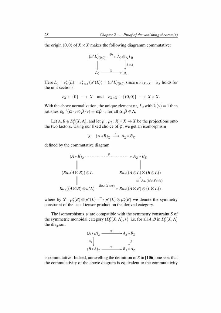
28 Chapter 2 – Proof of the vanishing theorem(s)
the origin (0,0) of X×X makes the following diagramm commutative:
(a∗L)(0,0)ϕ0 // L0⊗Λ L0
λ⊗λ
L0
λ // Λ
Here L0 = e∗X(L) = e∗X×X(a∗(L)) = (a∗L)(0,0) since aeX×X = eX holds for
the unit sections
eX : 0 −→ X and eX×X : (0,0) −→ X×X .
With the above normalization, the unique element v∈ L0 with λ (v) = 1 thensatisfies ϕ
−10 (α · v⊗β · v) = αβ · v for all α,β ∈ Λ.
Let A,B ∈ Dbc (X ,Λ), and let p1, p2 : X×X → X be the projections onto
the two factors. Using our fixed choice of ϕ , we get an isomorphism
ψ : (A∗B)χ
∼−→ Aχ ∗Bχ
defined by the commutative diagram
(A∗B)χ
ψ// Aχ ∗Bχ
(Ra∗(AB))⊗L Ra∗((A⊗L) (B⊗L))
Ra∗((AB)⊗a∗L)Ra∗(id⊗ϕ)
// Ra∗((AB)⊗ (LL))
∼= Ra∗(id⊗S′⊗id)
OO
where by S′ : p∗2(B)⊗ p∗1(L)∼−→ p∗1(L)⊗ p∗2(B) we denote the symmetry
constraint of the usual tensor product on the derived category.
The isomorphisms ψ are compatible with the symmetry constraint S ofthe symmetric monoidal category (Db
c (X ,Λ),∗), i.e. for all A,B in Dbc (X ,Λ)
the diagram
(A∗B)χ
Sχ
ψ // Aχ ∗Bχ
S
(B∗A)χ
ψ // Bχ ∗Aχ
is commutative. Indeed, unravelling the definition of S in [106] one sees thatthe commutativity of the above diagram is equivalent to the commutativity
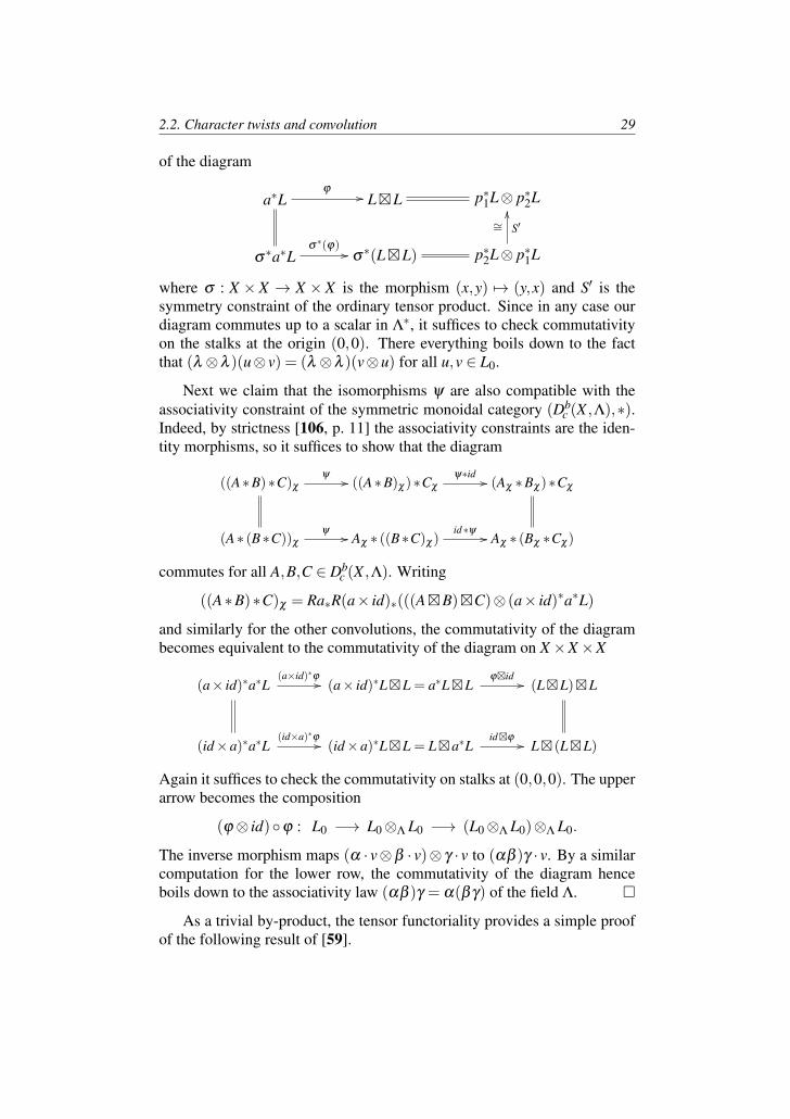
2.2. Character twists and convolution 29
of the diagram
a∗Lϕ
// LL p∗1L⊗ p∗2L
σ∗a∗Lσ∗(ϕ)
// σ∗(LL) p∗2L⊗ p∗1L
S′∼=OO
where σ : X × X → X × X is the morphism (x,y) 7→ (y,x) and S′ is thesymmetry constraint of the ordinary tensor product. Since in any case ourdiagram commutes up to a scalar in Λ∗, it suffices to check commutativityon the stalks at the origin (0,0). There everything boils down to the factthat (λ ⊗λ )(u⊗ v) = (λ ⊗λ )(v⊗u) for all u,v ∈ L0.
Next we claim that the isomorphisms ψ are also compatible with theassociativity constraint of the symmetric monoidal category (Db
c (X ,Λ),∗).Indeed, by strictness [106, p. 11] the associativity constraints are the iden-tity morphisms, so it suffices to show that the diagram
((A∗B)∗C)χ
ψ // ((A∗B)χ)∗Cχ
ψ∗id // (Aχ ∗Bχ)∗Cχ
(A∗ (B∗C))χ
ψ // Aχ ∗ ((B∗C)χ)id∗ψ // Aχ ∗ (Bχ ∗Cχ)
commutes for all A,B,C ∈ Dbc (X ,Λ). Writing
((A∗B)∗C)χ = Ra∗R(a× id)∗(((AB)C)⊗ (a× id)∗a∗L)
and similarly for the other convolutions, the commutativity of the diagrambecomes equivalent to the commutativity of the diagram on X×X×X
(a× id)∗a∗L(a×id)∗ϕ // (a× id)∗LL = a∗LL
ϕid // (LL)L
(id×a)∗a∗L(id×a)∗ϕ // (id×a)∗LL = La∗L
idϕ // L (LL)
Again it suffices to check the commutativity on stalks at (0,0,0). The upperarrow becomes the composition
(ϕ⊗ id)ϕ : L0 −→ L0⊗Λ L0 −→ (L0⊗Λ L0)⊗Λ L0.
The inverse morphism maps (α · v⊗β · v)⊗ γ · v to (αβ )γ · v. By a similarcomputation for the lower row, the commutativity of the diagram henceboils down to the associativity law (αβ )γ = α(βγ) of the field Λ.
As a trivial by-product, the tensor functoriality provides a simple proofof the following result of [59].
30 Chapter 2 – Proof of the vanishing theorem(s)
COROLLARY 2.2. For K ∈Dbc (X ,Λ) the Euler characteristic of Kχ does
not depend on the character χ .
Proof. In [106, lemma 8 on p. 28] it has been deduced from the Kunnethformula that hypercohomology defines a tensor functor ACU
H•(X ,−) : (Dbc (X ,Λ),∗) −→ (Vects
Λ,⊗s)
where the right hand side denotes the rigid symmetric monoidal categoryof super vector spaces over Λ, i.e. Z/2Z-graded vector spaces where thesymmetry constraint is twisted by the usual sign rule. Hence the Eulercharacteristic of K is equal, as an element of EndDb
c (X ,Λ)(1) = Λ, to thecomposite morphism
1coevK // K ∗K∨
SK,K∨ // K∨ ∗KevK // 1,
and as such it is invariant under character twists by proposition 2.1.
2.3. An axiomatic framework
Since the Tannakian constructions to be given below are of independentinterest also in more general situations than in the proof of theorem 1.1, forthe rest of this chapter we work in the following axiomatic setting. Considera Λ-linear rigid symmetric monoidal category (D,∗) whose unit object 1satisfies EndD(1)∼= Λ, and let
rat : (D,∗) −→ (Dbc (X ,Λ),∗)
be a faithful Λ-linear tensor functor ACU. The notation rat is motivated bythe case where k =C, Λ =Q and where D = Db(MHM(X)) is the boundedderived category of the category MHM(X) of mixed Hodge modules [89],but our formulation also applies to other situations.
For K ∈D we denote by H•(X ,K) resp. by χ(K) the hypercohomologyresp. the Euler characteristic of the sheaf complex rat(K). Similarly we usethe notation H•(X ,Kχ)=H•(X ,rat(K)χ) for twists by characters χ . Noticehowever that we do not assume the twisting functor lifts to the category D,so the formal token Kχ does not refer to an object in D. Depending on thecontext, we require the first four or all of the following axioms.
(D1) Degree shifts. We have an auto-equivalence K 7→ K[1] on D whichinduces the usual shift functor on Db
c (X ,Λ).
(D2) Perverse truncations. For n ∈ Z we have endofunctors pτ≤n, pτ≥non D and natural morphisms
pτ≤n(K) −→ K and K −→ p
τ≥n(K) for K ∈ D
which induce on Dbc (X ,Λ) the usual perverse truncations.
2.3. An axiomatic framework 31
Furthermore, the essential image P of the perverse cohomologyfunctors
pHn = pτ≤n p
τ≥n : D −→ P
is a full abelian subcategory of D, and rat : P−→ Perv(X ,Λ) is anexact functor between the respective abelian categories.
(D3) Perverse decomposition. For all K ∈ D we have a (non-canonical)isomorphism
K ∼=⊕n∈Z
pH−n(K)[n].
(D4) Semisimplicity. In (D2) the abelian category P is semisimple.
(D5) Hard Lefschetz. In D there exists an invertible object 1(1) whoseimage in Perv(X ,Λ) under rat is the Tate twist of 1. For all K,Lin D and all i≥ 0 we have functorial Lefschetz isomorphisms
pH−i(K ∗L) ∼= pH i(K ∗L)(i),
where the Tate twist (i) means i-fold convolution with 1(1).
We do not assume D to be triangulated, indeed we will later deal with thefollowing non-triangulated categories.
EXAMPLE 2.3. The axioms (D1) – (D5) hold if D ⊆ Dbc (X ,Λ) is the
full subcategory of all direct sums of degree shifts of semisimple perversesheaves which in case char(k)> 0 are defined over some finite field.
For k=C this follows from [35] together with [14], [43], or alternativelyfrom [87] and [78]. On the other hand, for char(k)> 0 one can invoke themixedness results of [69] and [10]. Note that in the above example we couldalso replace the category D by the full subcategory of objects of geometricorigin in the sense of [10, sect. 6.2.4].
EXAMPLE 2.4. The axioms (D1) – (D5) hold for k = C and Λ = Q ifone takes D to be the full subcategory of Db(MHM(X)) consisting of alldirect sums of degree shifts of semisimple Hodge modules.
In the above setting we consider a full subcategory N of D consistingof objects that are negligible for our purposes. In our later application thiswill be the category of objects which become isomorphic to zero in theAndre-Kahn quotient category D. Again, since we want to proceed as faras possible over a base field of arbitrary characteristic, we formulate therequired properties as the following axioms.
(N1) Stability. We have N∗D⊆N, and N is stable under taking retracts,degree shifts, perverse truncations and adjoint duals.
32 Chapter 2 – Proof of the vanishing theorem(s)
(N2) Twisting. Every object K ∈ N satisfies H•(X ,Kχ) = 0 for mostcharacters χ of the fundamental group.
(N3) Acyclicity. The category N contains all K ∈ D with H•(X ,K) = 0.
(N4) Euler characteristics. The category N contains all simple objectsof P whose Euler characteristic vanishes.
The meaning of these axioms will become clear later on. For the time beingwe content ourselves with the following
REMARK 2.5. Let Π be a set of characters of π1(X ,0), and N ⊆ D thefull subcategory of all K ∈ D such that rat(K) is a direct sum of degreeshifts of local systems Lχ with χ ∈Π. Then axioms (N1) and (N2) hold.
Proof. For any M ∈ Dbc (X ,Λ) we have Lχ ∗M = Lχ ⊗Λ H•(X ,Mχ−1)
by [106, p. 20], which in particular implies the stability property N∗D⊆Nso that axiom (N1) holds. For (N2) use that H•(X ,Lχ) = 0 if and only if thecharacter χ is non-trivial.
2.4. The Andre-Kahn quotient
For the Tannakian arguments to be given below, we want to work withrigid symmetric monoidal categories which are at the same time semisimpleabelian categories. To obtain such a category D that is as close as possibleto the triangulated category D, we will apply a general quotient constructionintroduced by Andre and Kahn in [1]. In what follows we always assumethat axioms (D1) – (D4) from the previous section, i.e. all axioms exceptfor the hard Lefschetz axiom, are satisfied.
The construction of Andre and Kahn works as follows. By rigidity wehave for each K ∈ D an isomorphism HomD(K,K)
∼−→ HomD(1,K ∗K∨)which in what follows we denote by f 7→ f ]. We then define the categoricaltrace tr( f ) ∈ EndD(1) = Λ of an endomorphism f ∈HomD(K,K) to be thecomposite morphism
tr( f ) : 1f ] // K ∗K∨
SK,K∨ // K∨ ∗KevK // 1
where as usual SK,K∨ denotes the symmetry constraint and evK denotes theevaluation morphism. Following section 7.1 of loc. cit. we then define theAndre-Kahn radical ND on objects K,L ∈ D by
ND(K,L) =
f ∈ HomD(K,L) | ∀g ∈ HomD(L,K) : tr(g f ) = 0.
This is an ideal of D in the sense that for all objects K,K′,L,L′ ∈ D and allmorphisms h1 ∈ HomD(K′,K), h2 ∈ HomD(L,L′) one can show
h2 ND(K,L)h1 ⊆ ND(K′,L′).
2.4. The Andre-Kahn quotient 33
For any ideal one has the notion of the corresponding quotient category. Bydefinition, the quotient
D = D/ND
has the same objects as D, but the morphisms in D between two objects K,Lare defined by
HomD(K,L) = HomD(K,L)/ND(K,L).
We have a natural quotient functor q : D−→D that is given by the identityon objects and by the quotient map on morphisms, and in what follows wedenote by P the essential image of P under this quotient functor. Recall thatultimately we want to construct a semisimple abelian category; as a firststep towards this goal we have
LEMMA 2.6. The quotient functor q : D −→ D preserves direct sums,and the category P is pseudo-abelian in the sense that every idempotentmorphism in it splits as the projection onto a direct summand.
Proof. The functor q preserves direct sums since it is Λ-linear. To seethat idempotents in P split, let P be an object of P. Since P is an abeliancategory and hence in particular pseudo-abelian, it suffices to show thatevery idempotent in
EndP(P) = EndP(P)/ND(P,P)
lifts to an idempotent in EndP(P). Since P is semisimple by axiom (D4),passing to isotypic components we can assume P = Q⊕r for some simpleobject Q of P and r ∈N. Then EndP(P) is the ring of r×r matrices over theskew field EndP(Q). Since matrix rings over skew fields do not have propertwo-sided ideals, it follows that either ND(P,P) = 0 or ND(P,P) = EndP(P),and in both cases the lifting of idempotents is obvious.
It turns out that this is already enough to conclude that the quotientcategory D has the desired properties:
PROPOSITION 2.7. The quotient category D is a semisimple abelianΛ-linear rigid symmetric monoidal category.
Proof. By [1, lemma 7.1.1] the Andre-Kahn radical ND is a monoidalideal in the sense that idM ∗ND(K,L)⊆ND(M∗K,M∗L) for all K,L,M ∈D,hence by sorite 6.1.4 of loc. cit. the quotient D = D/ND inherits from Dthe structure of a Λ-linear rigid symmetric monoidal category whose unitelement satisfies EndD(1) = Λ.
The main part of the proof is to check that the category D is semisimpleabelian. For this we first claim that
(?) HomD(P[m],Q[n]) = 0 for all objects P,Q in P and m 6= n.
34 Chapter 2 – Proof of the vanishing theorem(s)
Indeed, for m > n we even have HomD(P[m],Q[n]) = 0 since under thefaithful functor rat this Hom-group injects into
HomDbc (X ,Λ)(rat(P)[m],rat(Q)[n]) = Extn−m
Perv(X ,Λ)(rat(P),rat(Q))
which vanishes for m> n (for the above identification as an Ext-group recallthat Db
c (X ,Λ) is the derived category of Perv(X ,Λ)). On the other hand, inthe case m < n we have HomD(Q[n],P[m]) = 0, and then the definition ofthe Andre-Kahn radical implies that
HomD(P[m],Q[n]) = ND(P[m],Q[n])
which is mapped to zero under the quotient functor q : D −→ D. In bothcases the claim (?) follows.
Now by the perverse decomposition axiom (D3) every object K of Dcan be written as K =
⊕n∈ZKn[n] with certain Kn in P. For such K the
vanishing in (?) implies
(??) EndD(K) =⊕n∈Z
EndD(Kn[n]) =⊕n∈Z
EndP(Kn).
In particular, every idempotent endomorphism of K in the category D is adirect sum of idempotent endomorphisms of the summands Kn[n], and bylemma 2.6 it follows that D is pseudo-abelian. Hence to show that D is asemisimple abelian category, it will suffice by [1, A.2.10] to show that it isa semisimple Λ-linear category in the sense of section 2.1.1 in loc. cit. Forthis we use the following general result [2, th. 1].
Let F be a field and A an F-linear rigid symmetric monoidal categorywith EndA(1) = F . Suppose there exists an F-linear tensor functor ACUfrom A to an abelian F-linear rigid symmetric monoidal category V suchthat dimΛ(HomV(V1,V2))< ∞ for all V1,V2 ∈ V. Then the quotient of A byits Andre-Kahn radical NA is a semisimple F-linear category, and NA is theunique monoidal ideal of A with this property.
In our case this applies for F = Λ, A = D and for the functor H•(X ,−)from D to the abelian category V of super vector spaces over Λ.
COROLLARY 2.8. The functors P→ P and P → D are exact functorsbetween semisimple abelian categories. The image of a simple object P ∈ Pinside P is either simple or isomorphic to zero, and if Λ is algebraicallyclosed, then the latter case occurs if and only if χ(P) = 0.
Proof. By proposition 2.7, D is a semisimple abelian category, and italso follows from the proof of the proposition that P is a semisimple abeliansubcategory of D. Since the considered functors are additive, they are exactby semisimplicity. If P is a simple object of P, then EndP(P) is a skew field,
2.5. Super Tannakian categories 35
hence EndP(P) is a skew field or zero, and P is simple or zero in P. Overan algebraically closed field Λ there exist no skew fields other than Λ itself,hence in this case we have EndP(P) = Λ, and it follows that idP ∈ ND(P,P)iff tr(idP) = 0, which is the case iff χ(P) = 0.
COROLLARY 2.9. Let N⊆D be the full subcategory of all objects whichbecome isomorphic to zero in the quotient category D. If Λ is algebraicallyclosed, then N satisfies the stability axiom (N1), the acyclicity axiom (N3)and the Euler axiom (N4), and an object K ∈D lies in the subcategory N iffall simple constituents of all pHn(K) have Euler characteristic zero.
Proof. Property (N1) is obvious, property (N3) follows from (N4), andthe latter is immediate from corollary 2.8 by the perverse decompositionaxiom (D3) and the semisimplicity axiom (D4).
2.5. Super Tannakian categories
Using a criterion of Deligne, we now show that the semisimple abelianrigid symmetric monoidal category D from the previous section is almostTannakian: It is an inductive limit of super Tannakian categories, a notionthat we will recall below and in appendix A. In the case k = C we willsee later (in corollary 2.14, using that in this case the Euler characteristicof perverse sheaves is non-negative) that D is in fact an inductive limit ofordinary Tannakian categories, and this is closely related to our proof oftheorem 1.1. One may conjecture the same also for char(k)> 0.
Throughout this section we will always assume that Λ is algebraicallyclosed and that axioms (D1) – (D4) of section 2.3 hold. By semisimplicitythe convolution functor
∗ : D×D −→ Dis exact in each variable, and EndD(1) = Λ (this latter property is inheritedfrom D where it can be checked by applying the faithful functor rat). So Dis a categorie Λ-tensorielle in the sense of [30, sect. 0.1].
Recall that a full subcategory of D is said to be finitely tensor generatedif it is the category 〈K〉 consisting of all subquotients of convolution powersof K⊕K∨ for some fixed object K ∈ D. Our next goal is to show that anysuch subcategory is super Tannakian in the following sense.
The framework of algebraic geometry is generalized to super algebraicgeometry by replacing the category of commutative rings with the categoryof Z/2Z-graded super commutative rings. In particular one has the notionof an algebraic resp. reductive super group and its super representations, seeappendix A. For an algebraic super group G over Λ and a point ε ∈ G(Λ)with ε2 = 1 such that int(ε) is the parity automorphism of G, let us denote
36 Chapter 2 – Proof of the vanishing theorem(s)
by RepΛ(G,ε) the category of all super representations V = V0⊕V1 of Gover Λ such that ε acts by (−1)a on Va for a = 0,1. Categories of this formwill be called super Tannakian, with Tannaka super group G.
THEOREM 2.10. Any finitely generated full tensor subcategory 〈K〉 ⊂Dis super Tannakian, and its Tannaka super group G = G(K) is reductive.
Proof. Since D is a categorie Λ-tensorielle, for the first claim it sufficesby [30, th. 0.6] to see that for any object K ∈D and all n ∈N the number ofsimple constituents of (K⊕K∨)∗n in the semisimple abelian category D isat most Nn for some constant N = N(K) depending only on K. In the caseat hand one can take
N(K) = ∑i∈Z
dimΛ(H i(X ,M))
for any object M ∈ D that becomes isomorphic to K⊕K∨ in D, using theargument given in [110, top of p. 5]. Concerning reductivity, note that acategory RepΛ(G,ε) is semisimple iff G is reductive [108].
2.6. Perverse multiplier
We now introduce the notion of a multiplier. This will play an importantrole in our proof of theorem 1.1, indeed the theorem essentially amountsto the statement that any perverse sheaf on a complex abelian variety is amultiplier. In this section Λ need not be algebraically closed, but we assumeas always that axioms (D1) – (D4) from section 2.3 hold.
Let N be a full subcategory of D satisfying the stability axiom (N1). Wethen define an N-multiplier to be an object K ∈D such that for all r∈N0 andall n 6= 0 the subquotients of pHn((K⊕K∨)∗r) all lie in N. The relevance ofthis notion for theorem 1.1 is clear from
LEMMA 2.11. For P ∈ P the following holds.
(a) If the subcategory N satisfies the twisting axiom (N2) and if P isan N-multiplier, then H•(X ,Pχ) is concentrated in degree zero formost characters χ .
(b) Conversely, suppose that N satisfies the acyclicity axiom (N3) andthat the hard Lefschetz axiom (D5) holds. Then P is an N-multiplierif H•(X ,P) is concentrated in degree zero.
Proof. (a) Put g = dim(X). The perverse decomposition axiom (D3)shows that
P∗(g+1) =⊕m∈Z
Pm[m] for suitable Pm ∈ P .
2.6. Perverse multiplier 37
By assumption P is an N-multiplier, hence Pm ∈ N for all m 6= 0. Via thetwisting axiom (N2) it follows that for most characters χ and all n ∈ Z,
Hn(X ,P∗(g+1)χ ) = Hn(X ,(P0)χ).
The right hand side vanishes for |n|> g since rat(P0)χ is perverse. But forthe left hand side we have
H•(X ,P∗(g+1)χ ) = (H•(X ,Pχ))
⊗(g+1)
by proposition 2.1 and since H•(X ,−) is a tensor functor by the Kunneththeorem. So the above vanishing statement for |n|> g implies that H•(X ,Pχ)is concentrated in degree zero.
(b) Put Q = (P⊕ P∨)∗r for any r ∈ N. Since hypercohomology is atensor functor by the Kunneth theorem, with H•(X ,Pχ) also H•(X ,Q) isconcentrated in degree zero. Using the hard Lefschetz axiom (D5), onethen deduces that for all n 6= 0 one has H•(X , pHn(Q)) = 0 so that by (N3)the subcategory N contains pHn(Q). Since this holds for arbitrary r ∈ N, itfollows that P is an N-multiplier.
In view of part (a) of the lemma, to prove theorem 1.1 we want to showthat for a suitable subcategory N every object of P is an N-multiplier. Forthis we will argue by contradiction, using the following
LEMMA 2.12. Suppose that N satisfies the stability axiom (N1) and theEuler axiom (N4), that D satisfies all axioms (D1) – (D5) and that P ∈ P isnot an N-multiplier. Then for some r ∈ N the convolution power
(P∗P∨)∗r = (P∗P∨)∗ · · · ∗ (P∗P∨)
admits a direct summand of the form 1[2i](i) with an integer i 6= 0.
Proof. If P is not an N-multiplier, we can find integers a,b ∈ N suchthat P∗a ∗ (P∨)∗b admits a direct summand Q[i] for some i 6= 0 and somesimple object Q ∈ P which is not in N. By the hard Lefschetz axiom (D5)then Q[−i](−i) is a direct summand of P∗a ∗ (P∨)∗b as well. It then followsthat also the dual Q∨[i](i) is a direct summand of P∗b ∗ (P∨)∗a. Altogetherthen the convolution product Q[i]∗Q∨[i](i) = Q∗Q∨[2i](i) will be a directsummand of (P∗P∨)∗r for the exponent r = a+b.
It remains to show that 1 is a direct summand of Q ∗Q∨. For this notethat the trace map tr(Q) : 1 −→ Q ∗Q∨ ∼= Q∨ ∗Q −→ 1 is non-zero sincewe have χ(Q) 6= 0 by axiom (N4). Now tr(Q) factors over pH0(Q ∗Q∨),indeed HomD(P, pτ>0P) = HomD(
pτ<0P,P) = 0. So tr(Q) exhibits 1 as aretract of pH0(Q∗Q∨) in the abelian category P, and we are done.
38 Chapter 2 – Proof of the vanishing theorem(s)
2.7. The main argument
To finish the proof of theorem 1.1 we will control the non-perversity ofconvolution products such as in lemma 2.12 via central characters of theTannaka super group introduced in theorem 2.10. By devissage we canrestrict ourselves to semisimple perverse sheaves as in example 2.3. Sosuppose that Λ = C or Λ = Ql and that D satisfies all axioms (D1) – (D5)of section 2.3. Consider the semisimple abelian rigid symmetric monoidalquotient category D from section 2.4.
For the full subcategory N⊆D of all objects that become isomorphic tozero in D, the stability axiom (N1), the acyclicity axiom (N3) and the Euleraxiom (N4) are satisfied as we have seen in corollary 2.9. In the setting ofexample 2.3 presumably also the twisting axiom (N2) always holds; at leastover the base field k = C we have shown this in corollary 1.7. Hence inthe complex case part (a) of lemma 2.11 can be applied using the twistingaxiom (N2), and then theorem 1.1 follows from axioms (N1) and (N4) viathe following argument from representation theory.
THEOREM 2.13. Let N⊆D be a full subcategory satisfying the stabilityaxiom (N1) and the Euler axiom (N4). Then every P ∈ P is an N-multiplier.
Proof. Suppose that P ∈ P is simple and not an N-multiplier. Then forsome integer r ∈ N the convolution (P ∗P∨)∗r contains by lemma 2.12 adirect summand L = 1[2i](i) with i 6= 0. In particular, it follows that the fullrigid symmetric monoidal subcategory D1 ⊂ D generated by the object Pcontains the full rigid symmetric monoidal subcategory D0 ⊂ D generatedby the invertible object L.
Theorem 2.10 shows that for certain reductive super groups Gi over Λ
we have tensor equivalences ωi : Di∼−→ RepΛ(Gi,εi) for i ∈ 0,1, and by
the Tannakian formalism the inclusion of categories D0 ⊆ D1 defines anepimorphism of reductive super groups
h : G1 G0.
The category D0 consists of all direct sums of skyscraper sheaves L∗n withintegers n ∈ Z, where by a negative power we mean the correspondingpower of the dual. Since L∗n ∼= 1[2ni](ni) and i 6= 0, equation (??) in theproof of proposition 2.7 implies that one has an isomorphism L∗n ∼= 1 in Donly if n = 0. Thus the tensor equivalence ω0 between D0 and RepΛ(G0,ε0)is realized explicitly with G0 =Gm and ε0 =−1 via
L∗n 7→ (the character z 7→ zn of Gm).
In particular, the representation W0 = ω0(L) is non-trivial, corresponding tothe identity character z 7→ z of the multiplicative group Gm.
2.7. The main argument 39
But proposition A.3 in the appendix applies to the torus T0 = G0 =Gm,so there exists a central torus T1 ∼=Gm in G1 such that h : G1G0 restrictsto an isogeny T1→ T0. By Schur’s lemma the central torus T1 acts via somecharacter on the irreducible super representation W1 = ω1(P), so T1 actstrivially on W1⊗W∨1 = ω1(P ∗P∨). Hence T1 acts trivially on the directsummand
W0 ⊆ (W1⊗W∨1 )⊗r
and therefore also T0 acts trivially on W0 = ω0(L), a contradiction.
COROLLARY 2.14. If the base field k is C, then the super group G(K)in theorem 2.10 is a classical reductive algebraic group.
Proof. Corollary 2.9 and theorem 2.13 show that the category P is stableunder convolution. Using this one easily reduces our claim to the specialcase where K lies inside P. In this case, all objects of RepΛ(G(K),ε) havenon-negative dimension because over the ground field k = C we have seenin section 1.4 that χ(P) ≥ 0 for all perverse sheaves P ∈ Perv(X ,Λ). Theassertion then follows from [31, th. 7.1].

CHAPTER 3
Perverse sheaves on semiabelian varieties
The Tannaka groups in corollary 2.14 provide a new tool for the studyof smooth projective varieties with non-trivial Albanese morphism. Theirrepresentation theory can be considered as a substitute for Brill-Noethertheory in higher dimensions, and they are also closely related to the moduliof abelian varieties as we will discuss in chapter 4. However, in generalthese Tannaka groups are hard to compute. At present the most effectivetool to determine them is to study degenerations of the underlying abelianvariety; even if one is only interested in semisimple perverse sheaves onabelian varieties, this naturally leads to non-semisimple perverse sheaveson semiabelian varieties. In this chapter we extend our previous Tannakianconstructions to this more general case, combining arguments of Gabberand Loeser for tori [41] with the generic vanishing theorem 1.1 for abelianvarieties. For degenerations of abelian varieties into semiabelian varietieswe then show that the nearby cycles functor induces an embedding of thedegenerate Tannaka group into the generic one whenever one can possiblyexpect this (see theorem 3.15). Finally, we also discuss how the obtainedTannaka groups vary in families on abelian schemes.
Before we come to the details, let us begin with a brief overview overthe constructions that follow. Throughout we work over an algebraicallyclosed field k of any characteristic p≥ 0. Let X be a semiabelian variety, acommutative group variety which is an extension
1−→ T −→ X −→ A−→ 1
of an abelian variety A by an algebraic torus T over k. Fixing a prime l 6= p,we put Λ =Ql and denote by
D = D(X) = Dbc (X ,Λ) and P = P(X) = Perv(X ,Λ)
the triangulated category of bounded constructible Λ-sheaf complexes resp.its full abelian subcategory of perverse sheaves. Let m : X ×k X −→ X bethe group law. In the non-proper case we have two different notions ofconvolution which are given by
K ∗! L = Rm!(KL) and K ∗∗ L = Rm∗(KL)
for K,L ∈ D. In general the abelian subcategory P ⊂ D will of course notbe stable under these two convolution products. Motivated by the results of
41
42 Chapter 3 – Perverse sheaves on semiabelian varieties
the previous chapter, we consider the full subcategory T ⊂ D of all sheafcomplexes K ∈ D which are negligible in the sense that for all n ∈ Z theperverse cohomology sheaves pHn(K) have Euler characteristic zero. Overthe base field k = C we will see that
(a) the triangulated quotient category D = D/T exists (corollary 3.6),(b) both ∗! and ∗∗ descend to the same bifunctor ∗ : D×D−→D which
preserves the essential image P⊂ D of P (theorem 3.8),(c) with ∗ as its tensor product, the category P is an inductive limit of
neutral Tannakian categories (corollary 3.10).
Recall [33, th. 2.11] that a neutral Tannakian category is a category whichis equivalent to the category RepΛ(G) of linear representations of an affinegroup scheme G over Λ. In particular, to any perverse sheaf P ∈ P we willattach an affine algebraic group G = G(P) over Λ which corresponds tothe tensor subcategory 〈P〉 ⊂ P generated by P under convolution. Since Λ
is algebraically closed, the group G(P) is determined uniquely by P up toisomorphism. These are the Tannaka groups we are interested in and whosedegeneration behaviour will be studied in theorem 3.15.
For algebraic tori X = T the properties (a) – (c) have been obtainedin [41, sect. 3.6 – 3.7] via the Mellin transform as a consequence of Artin’saffine vanishing theorem, and our arguments in sections 3.1 through 3.4 areheavily indebted by loc. cit. However, for abelian varieties X = A we nolonger dispose of Artin’s vanishing theorem. Over the complex numberswe can instead apply our vanishing theorem 1.1 which is in fact closelyrelated with the Tannakian property as we have seen in chapter 2. Eventhough at present we can prove this vanishing theorem only over k = C, itis likely to hold in positive characteristic as well. So in what follows weformulate it as an axiomatic assumption under which our arguments workover an algebraically closed field k of arbitrary characteristic.
3.1. Vanishing theorems revisited
To formulate the generic vanishing axiom that generalizes theorem 1.1to the non-proper case over a field k of arbitrary characteristic, we considercharacters of the tame fundamental group. As a base point we will alwaystake the neutral element 0 ∈ X(k). Recall from [97, sect. 1.3] that everysemiabelian variety X has a smooth compactification with a normal crossingboundary divisor. The tame fundamental group π t
1(X ,0) classifies the finiteetale covers of X that are tamely ramified along each component of sucha boundary divisor, see [51, exp. XIII, sect. 2 and 5], [52] and [93]. Inparticular π t
1(X ,0) is a quotient of the etale fundamental group π1(X ,0),and equal to it if the field k has characteristic zero or if X is proper.
3.1. Vanishing theorems revisited 43
The group Π(X) of continuous characters χ : π t1(X ,0)−→ Λ∗ admits a
natural product decomposition
Π(X) = Π(X)l′×Π(X)l,
whereΠ(X)l′ = χ ∈Π(X) : χ
n = 1 for some n with l - n
denotes the subgroup of all characters of finite order prime to l and where bydefinition Π(X)l is the group of all characters that factor over the maximalpro-l-quotient π1(X ,0)l = π t
1(X ,0)l . The latter is a free Zl-module of finiterank [17]. So with the same arguments as in [41, sect. 3.2] the set Π(X)lof pro-l-characters can be identified with the set of Λ-valued points of ascheme in a natural way (even though as in loc. cit. the multiplication ofcharacters does not come from a group scheme structure). This being said,we consider the set of all tame characters
Π(X) =∐
χ∈Π(X)l′
χ ·Π(X)l
as the disjoint union of the infinitely many components χ ·Π(X)l indexedby the torsion characters χ ∈Π(X)l′ , and we say that a statement holds fora generic character if it holds for all characters in an open subset of Π(X)that is dense in each of these components.
For sheaf complexes K ∈D(X) and characters χ ∈Π(X) we consider asin the previous chapters the twist Kχ =K⊗Λ Lχ by the local system Lχ . OurTannakian constructions will be based on the following generic vanishingassumption for such character twists.
ASSUMPTION GV(X). Let P ∈ P(X). Then for generic χ ∈ Π(X) theforget support map
H•c (X ,Pχ) −→ H•(X ,Pχ)
is an isomorphism, and
H i(X ,Pχ) = H ic(X ,Pχ) = 0 for all i 6= 0.
For complex abelian varieties this is precisely the content of the genericvanishing theorem 1.1, the claim about the forget support map being trivialin that case. At present we do not know whether the assumption GV (X) alsoholds for abelian varieties over an algebraically closed field k of positivecharacteristic p = char(k)> 0, but in any case the semiabelian version canbe deduced from the abelian one as follows.
THEOREM 3.1. If the maximal abelian variety quotient A = X/T of Xsatisfies the assumption GV (A), then also GV (X) holds.
44 Chapter 3 – Perverse sheaves on semiabelian varieties
Proof. We first claim that for any given perverse sheaf P ∈ P(X), the setof all characters χ which violate the conditions in our assumption GV (X)forms a closed subset of the scheme Π(X). To see this, consider the Mellintransforms M!(P) and M∗(P) as defined in [41, sect. 3.3] (in loc. cit. thedefinition is only given for algebraic tori, but it carries over verbatim to thecase at hand). These Mellin transforms are objects of the bounded derivedcategory of coherent sheaves on Π(X) with the property that for all i ∈ Zand any character χ ∈Π(X) we have isomorphisms
H ic(X ,Pχ) ∼= H i(Li∗χM!(P)),
H i(X ,Pχ) ∼= H i(Li∗χM∗(P)),
where iχ : χ →Π(X) denotes the embedding of the closed point given bythe chosen character. Furthermore, we have a morphism M!(P)−→M∗(P)which induces via the above identifications the forget support morphism oncohomology. Since on a Noetherian scheme the support of any coherentsheaf is a closed subset, it follows that the locus of all characters χ whichviolate GV (X) forms a closed subset S (P)⊆Π(X) as claimed.
We must show that under the assumption GV (A) the complement of thisclosed subset S (P) meets every irreducible component of Π(X). So wemust see that for at least one character χ in each component the propertiesin GV (X) hold. To this end consider the exact sequence
0 −→ T i−→ Xf−→ A −→ 0
which defines the given semiabelian variety. Lemma 3.2 below will showthat every component of Π(X) contains a character χ such that the forgetsupport morphism
R f!(Pχ) −→ R f∗(Pχ)
is an isomorphism. In this case Artin’s vanishing theorem for the affinemorphism f also shows that these two isomorphic direct image complexesare perverse [41, lemma 2.4]. For all ϕ ∈Π(A) and ψ = f ∗(ϕ) ∈Π(X) theprojection formula furthermore says
(R f!(Pχ))ϕ = R f!(Pχψ) and (R f∗(Pχ))ϕ = R f∗(Pχψ),
hence we are finished by an application of the vanishing assumption GV (A)to these perverse direct images.
To fill in the missing statement in the above proof, we consider the givensemiabelian variety as a torsor f : X −→ A under the torus T in the senseof [74, sect. III.4]. The condition of being a torsor is satisfied since clearlythe morphism X ×k T −→ X ×A X , (x, t) 7→ (x,xt) is an isomorphism. Theresult we are looking for only uses the structure as a torsor, and for its proofit will be convenient to forget that our base A is an abelian variety. So wewill work in the following setting.
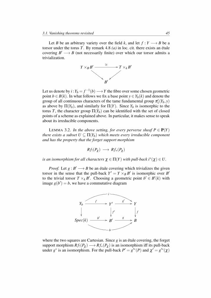
3.1. Vanishing theorems revisited 45
Let B be an arbitrary variety over the field k, and let f : Y −→ B be atorsor under the torus T . By remark 4.8 (a) in loc. cit. there exists an etalecovering B′ −→ B (not necessarily finite) over which our torsor admits atrivialization.
Y ×B B′∼= //
##GGG
GGGG
GGT ×k B′
xxxx
xxxx
x
B′
Let us denote by i : Yb = f−1(b)−→Y the fibre over some chosen geometricpoint b ∈ B(k). In what follows we fix a base point y ∈Yb(k) and denote thegroup of all continuous characters of the tame fundamental group πt
1(Yb,y)as above by Π(Yb), and similarly for Π(Y ). Since Yb is isomorphic to thetorus T , the character group Π(Yb) can be identified with the set of closedpoints of a scheme as explained above. In particular, it makes sense to speakabout its irreducible components.
LEMMA 3.2. In the above setting, for every perverse sheaf P ∈ P(Y )there exists a subset U ⊆ Π(Yb) which meets every irreducible componentand has the property that the forget support morphism
R f!(Pχ) −→ R f∗(Pχ)
is an isomorphism for all characters χ ∈Π(Y ) with pull-back i∗(χ) ∈U.
Proof. Let g : B′ −→ B be an etale covering which trivializes the giventorsor in the sense that the pull-back Y ′ = Y ×B B′ is isomorphic over B′
to the trivial torsor T ×k B′. Choosing a geometric point b′ ∈ B′(k) withimage g(b′) = b, we have a commutative diagram
Ybi′ //
i
%%Y ′
f ′
g′ // Y
f
Spec(k) b′ //
b
99B′g // B
where the two squares are Cartesian. Since g is an etale covering, the forgetsupport morphism R f!(Pχ)−→ R f∗(Pχ) is an isomorphism iff its pull-backunder g∗ is an isomorphism. For the pull-back P′ = g′∗(P) and χ ′ = g′∗(χ)
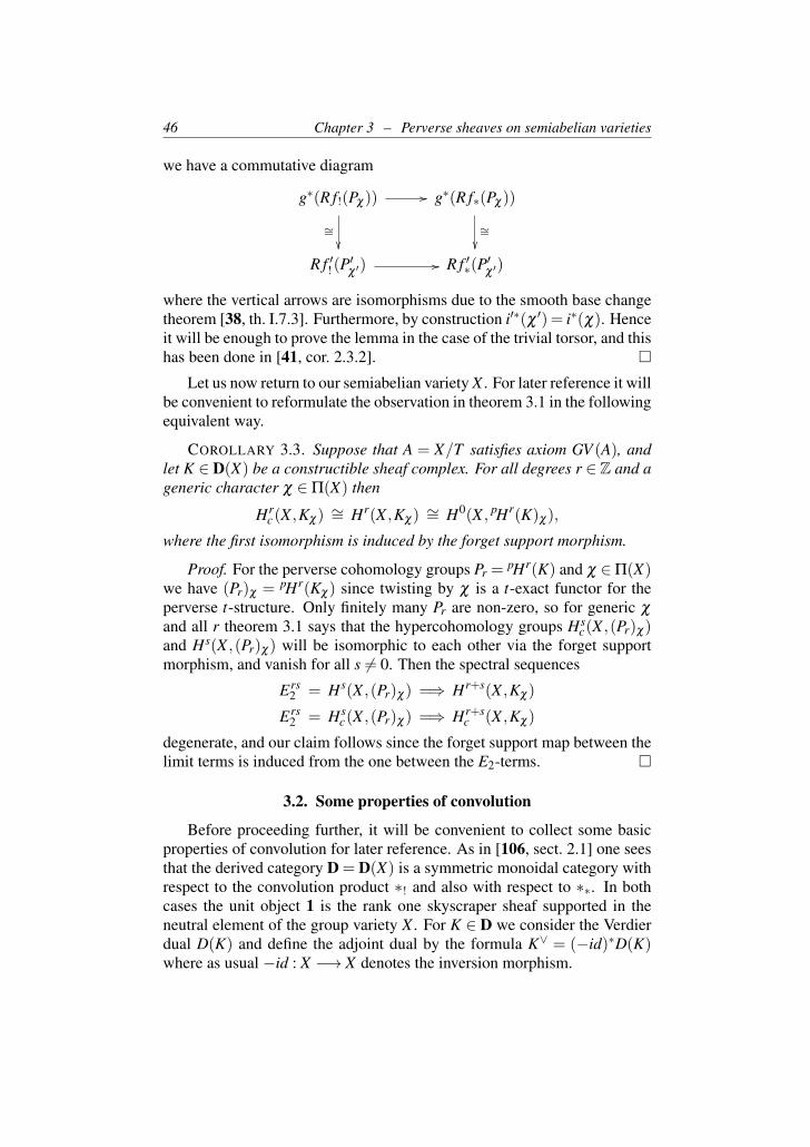
46 Chapter 3 – Perverse sheaves on semiabelian varieties
we have a commutative diagram
g∗(R f!(Pχ)) //
∼=
g∗(R f∗(Pχ))
∼=
R f ′! (P′χ ′) // R f ′∗(P
′χ ′)
where the vertical arrows are isomorphisms due to the smooth base changetheorem [38, th. I.7.3]. Furthermore, by construction i′∗(χ ′) = i∗(χ). Henceit will be enough to prove the lemma in the case of the trivial torsor, and thishas been done in [41, cor. 2.3.2].
Let us now return to our semiabelian variety X . For later reference it willbe convenient to reformulate the observation in theorem 3.1 in the followingequivalent way.
COROLLARY 3.3. Suppose that A = X/T satisfies axiom GV (A), andlet K ∈D(X) be a constructible sheaf complex. For all degrees r ∈ Z and ageneric character χ ∈Π(X) then
Hrc(X ,Kχ) ∼= Hr(X ,Kχ) ∼= H0(X , pHr(K)χ),
where the first isomorphism is induced by the forget support morphism.
Proof. For the perverse cohomology groups Pr =pHr(K) and χ ∈Π(X)
we have (Pr)χ = pHr(Kχ) since twisting by χ is a t-exact functor for theperverse t-structure. Only finitely many Pr are non-zero, so for generic χ
and all r theorem 3.1 says that the hypercohomology groups Hsc(X ,(Pr)χ)
and Hs(X ,(Pr)χ) will be isomorphic to each other via the forget supportmorphism, and vanish for all s 6= 0. Then the spectral sequences
Ers2 = Hs(X ,(Pr)χ) =⇒ Hr+s(X ,Kχ)
Ers2 = Hs
c(X ,(Pr)χ) =⇒ Hr+sc (X ,Kχ)
degenerate, and our claim follows since the forget support map between thelimit terms is induced from the one between the E2-terms.
3.2. Some properties of convolution
Before proceeding further, it will be convenient to collect some basicproperties of convolution for later reference. As in [106, sect. 2.1] one seesthat the derived category D = D(X) is a symmetric monoidal category withrespect to the convolution product ∗! and also with respect to ∗∗. In bothcases the unit object 1 is the rank one skyscraper sheaf supported in theneutral element of the group variety X . For K ∈ D we consider the Verdierdual D(K) and define the adjoint dual by the formula K∨ = (−id)∗D(K)where as usual −id : X −→ X denotes the inversion morphism.
3.3. The thick subcategory of negligible objects 47
LEMMA 3.4. For all K,M ∈ D and χ ∈ Π(X) one has the followingnatural isomorphisms.
(a) Adjoint duality:
HomD(1,K∨ ∗∗M) ∼= HomD(K,M) ∼= HomD(K ∗! M∨,1).
(b) Character twists:(Kχ)
∨ ∼= (K∨)χ ,
(K ∗! M)χ∼= Kχ ∗! Mχ and (K ∗∗M)χ
∼= Kχ ∗∗Mχ .
(c) Verdier duality:
D(K ∗! M) ∼= D(K)∗∗D(M), D(K ∗∗M) ∼= D(K)∗! D(M).
(d) Kunneth formulae:
H•c (X ,K)⊗Λ H•c (X ,M)∼−→ H•c (X ,K ∗! M),
H•(X ,K ∗∗M)∼−→ H•(X ,K)⊗Λ H•(X ,M).
Proof. Part (a) follows from adjunction as in [41, p. 533]. In (b) thefirst identity comes from RHom(Lχ ,ΛX) = Lχ−1 and (−id)∗(Lχ−1) = Lχ ,and the other two follow as in proposition 2.1. Part (c) follows from thecompatibility of Verdier duality with exterior tensor products. Part (d) isthe Kunneth isomorphism [7, exp. XVII.5.4] resp. its Verdier dual.
3.3. The thick subcategory of negligible objects
In this and in the next section we always assume that for the abelianvariety A = X/T the vanishing assumption GV (A) of section 3.1 holds. Wehave seen in theorem 3.1 that GV (X) then holds as well. Let S(X)⊂ P(X)be the full subcategory of all perverse sheaves of Euler characteristic zero,and T(X) ⊂ D(X) the full subcategory of all sheaf complexes K whoseperverse cohomology sheaves pHn(K) lie in S(X) for all degrees n ∈ Z. Forbrevity we put
P = P(X), D = D(X), S = S(X) and T = T(X).
The following explains why we only use characters of the tame fundamentalgroup — we want the Euler characteristic χ(K) = ∑i∈Z dimΛ(H i(X ,K)) ofany complex K ∈ D to be invariant under character twists.
LEMMA 3.5. Let K ∈ D. Then χ(K) = χ(Kϕ) for all ϕ ∈Π(X), hencethe following three conditions are equivalent:
(a) The complex K lies in the full subcategory T.(b) We have H•(X ,Kϕ) = 0 for generic ϕ ∈Π(X).(c) We have H•c (X ,Kϕ) = 0 for generic ϕ ∈Π(X).
48 Chapter 3 – Perverse sheaves on semiabelian varieties
Proof. To prove the twist invariance of the Euler characteristic, we canby devissage assume that the complex K is a constructible sheaf placed ina single cohomology degree. Then [59, cor. 2.9] says that if j : X → Xdenotes a smooth compactification, then j!(K) and j!(Kϕ) have the sameEuler characteristic (the assumptions of the corollary are satisfied since χ isa tame character, see sect. 2.6 of loc. cit.). Since for the Euler characteristicit makes no difference whether we use compactly supported or ordinaryhypercohomology [70], it follows that χ(K) = χ(Kϕ). The equivalence ofthe three conditions (a) – (c) then follows via corollary 3.3.
Recall that a full subcategory of an abelian category is said to be a Serresubcategory if it is stable under the formation of arbitrary subquotients andextensions. More generally, a full triangulated subcategory of a triangulatedcategory is called a thick subcategory if it has the following property: Forany morphism f : K → L which factors over an object of the subcategoryand has its cone in the subcategory, the objects K and L must both belongto the subcategory as well.
COROLLARY 3.6. The subcategory S⊂ P is Serre, and T⊂ D is thick.
Proof. Let 0−→ P−→ Q−→ R−→ 0 be a short exact sequence in theabelian category P. Theorem 3.1 says that for a generic character χ ∈Π(X)the hypercohomology of the perverse sheaves Pχ , Qχ and Rχ is concentratedin degree zero so that the long exact sequence in hypercohomology reducesto a short exact sequence
0−→ H0(X ,Pχ)−→ H0(X ,Qχ)−→ H0(X ,Rχ)−→ 0.
Therefore lemma 3.5 shows that Q lies in S if and only if both P and R arein S. Hence S ⊂ P is a Serre subcategory, and then the subcategory T ⊂ Dis thick by [41, prop. 3.6.1(i)].
In particular, localizing the abelian category P at the class of morphismswhose kernel and cokernel lie in the Serre subcategory S we can form theabelian quotient category P = P/S in the sense of [42, chap. III]. Note thatthe category P has the same objects as P and that for any objects P1,P2the elements of HomP(P1,P2) can be represented by equivalence classes ofdiagrams in P of the form
Qf1zzuuuuuu f2
$$IIIIII
P1 P2
where the kernel and cokernel of the morphism f1 lie in S. In the sameway, localizing the triangulated category D at the class of morphisms whosecone lies in the thick subcategory T we can form the triangulated quotientcategory D = D/T as described in [82, sect. 2.1].
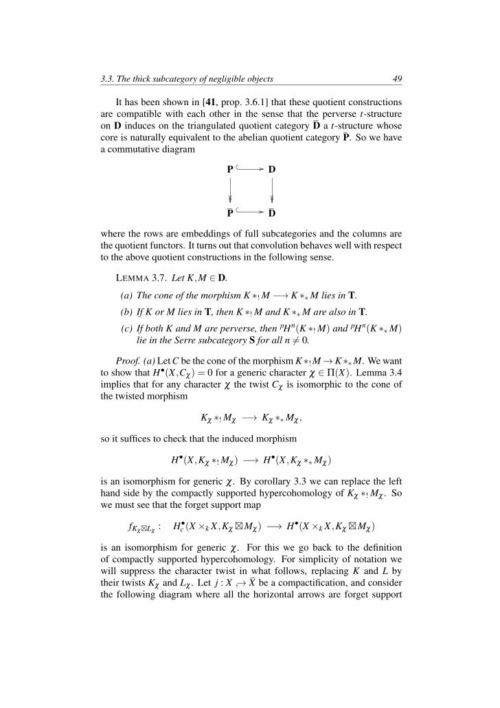
3.3. The thick subcategory of negligible objects 49
It has been shown in [41, prop. 3.6.1] that these quotient constructionsare compatible with each other in the sense that the perverse t-structureon D induces on the triangulated quotient category D a t-structure whosecore is naturally equivalent to the abelian quotient category P. So we havea commutative diagram
P //
D
P // D
where the rows are embeddings of full subcategories and the columns arethe quotient functors. It turns out that convolution behaves well with respectto the above quotient constructions in the following sense.
LEMMA 3.7. Let K,M ∈ D.
(a) The cone of the morphism K ∗! M −→ K ∗∗M lies in T.
(b) If K or M lies in T, then K ∗! M and K ∗∗M are also in T.
(c) If both K and M are perverse, then pHn(K ∗! M) and pHn(K ∗∗M)lie in the Serre subcategory S for all n 6= 0.
Proof. (a) Let C be the cone of the morphism K∗! M→K∗∗M. We wantto show that H•(X ,Cχ) = 0 for a generic character χ ∈ Π(X). Lemma 3.4implies that for any character χ the twist Cχ is isomorphic to the cone ofthe twisted morphism
Kχ ∗! Mχ −→ Kχ ∗∗Mχ ,
so it suffices to check that the induced morphism
H•(X ,Kχ ∗! Mχ) −→ H•(X ,Kχ ∗∗Mχ)
is an isomorphism for generic χ . By corollary 3.3 we can replace the lefthand side by the compactly supported hypercohomology of Kχ ∗! Mχ . Sowe must see that the forget support map
fKχLχ: H•c (X×k X ,Kχ Mχ) −→ H•(X×k X ,Kχ Mχ)
is an isomorphism for generic χ . For this we go back to the definitionof compactly supported hypercohomology. For simplicity of notation wewill suppress the character twist in what follows, replacing K and L bytheir twists Kχ and Lχ . Let j : X → X be a compactification, and considerthe following diagram where all the horizontal arrows are forget support
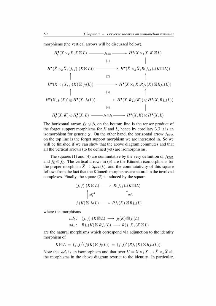
50 Chapter 3 – Perverse sheaves on semiabelian varieties
morphisms (the vertical arrows will be discussed below).
H•c (X×k X ,KL) fKL // H•(X×k X ,KL)
H•(X×k X ,( j, j)!(KL)) //
(1)
H•(X×k X ,R( j, j)∗(KL))
H•(X×k X , j!(K) j!(L)) //
OO(2)
H•(X×k X ,R j∗(K)R j∗(L))
OO
H•(X , j!(K))⊗H•(X , j!(L)) //
OO(3)
H•(X ,R j∗(K))⊗H•(X ,R j∗(L))
OO
H•c (X ,K)⊗H•c (X ,L) fK⊗ fL //
(4)
H•(X ,K)⊗H•(X ,L)
The horizontal arrow fK ⊗ fL on the bottom line is the tensor product ofthe forget support morphisms for K and L, hence by corollary 3.3 it is anisomorphism for generic χ . On the other hand, the horizontal arrow fKLon the top line is the forget support morphism we are interested in. So wewill be finished if we can show that the above diagram commutes and thatall the vertical arrows (to be defined yet) are isomorphisms.
The squares (1) and (4) are commutative by the very definition of fKLand fK ⊗ fL. The vertical arrows in (3) are the Kunneth isomorphisms forthe proper morphism X → Spec(k), and the commutativity of this squarefollows from the fact that the Kunneth morphisms are natural in the involvedcomplexes. Finally, the square (2) is induced by the square
( j, j)!(KL) // R( j, j)∗(KL)
j!(K) j!(L) //
ad−1!
OO
R j∗(K)R j∗(L)
ad∗
OO
where the morphisms
ad! : ( j, j)!(KL) −→ j!(K) j!(L)
ad∗ : R j∗(K)R j∗(L) −→ R( j, j)∗(KL)
are the natural morphisms which correspond via adjunction to the identitymorphism of
KL = ( j, j)!( j!(K) j!(L)) = ( j, j)∗(R j∗(K)R j∗(L)).
Note that ad! is an isomorphism and that over U = X ×k X → X ×k X allthe morphisms in the above diagram restrict to the identity. In particular,
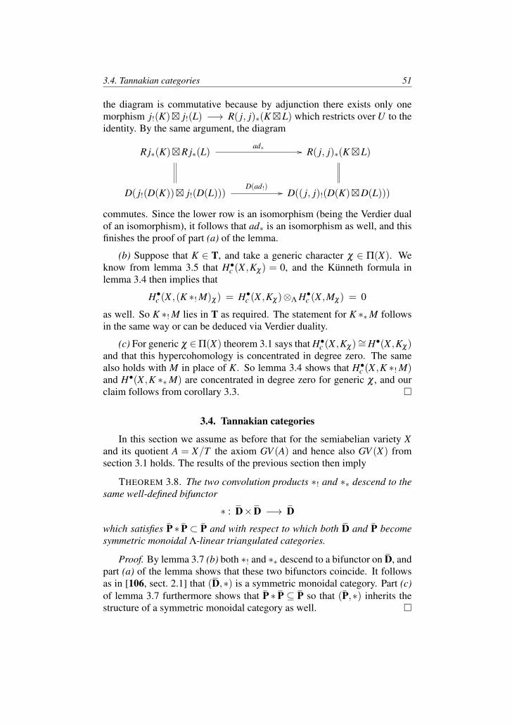
3.4. Tannakian categories 51
the diagram is commutative because by adjunction there exists only onemorphism j!(K) j!(L) −→ R( j, j)∗(KL) which restricts over U to theidentity. By the same argument, the diagram
R j∗(K)R j∗(L)ad∗ // R( j, j)∗(KL)
D( j!(D(K)) j!(D(L)))D(ad!) // D(( j, j)!(D(K)D(L)))
commutes. Since the lower row is an isomorphism (being the Verdier dualof an isomorphism), it follows that ad∗ is an isomorphism as well, and thisfinishes the proof of part (a) of the lemma.
(b) Suppose that K ∈ T, and take a generic character χ ∈ Π(X). Weknow from lemma 3.5 that H•c (X ,Kχ) = 0, and the Kunneth formula inlemma 3.4 then implies that
H•c (X ,(K ∗! M)χ) = H•c (X ,Kχ)⊗Λ H•c (X ,Mχ) = 0
as well. So K ∗! M lies in T as required. The statement for K ∗∗M followsin the same way or can be deduced via Verdier duality.
(c) For generic χ ∈Π(X) theorem 3.1 says that H•c (X ,Kχ)∼= H•(X ,Kχ)and that this hypercohomology is concentrated in degree zero. The samealso holds with M in place of K. So lemma 3.4 shows that H•c (X ,K ∗! M)and H•(X ,K ∗∗M) are concentrated in degree zero for generic χ , and ourclaim follows from corollary 3.3.
3.4. Tannakian categories
In this section we assume as before that for the semiabelian variety Xand its quotient A = X/T the axiom GV (A) and hence also GV (X) fromsection 3.1 holds. The results of the previous section then imply
THEOREM 3.8. The two convolution products ∗! and ∗∗ descend to thesame well-defined bifunctor
∗ : D×D −→ D
which satisfies P ∗P ⊂ P and with respect to which both D and P becomesymmetric monoidal Λ-linear triangulated categories.
Proof. By lemma 3.7 (b) both ∗! and ∗∗ descend to a bifunctor on D, andpart (a) of the lemma shows that these two bifunctors coincide. It followsas in [106, sect. 2.1] that (D,∗) is a symmetric monoidal category. Part (c)of lemma 3.7 furthermore shows that P ∗P ⊆ P so that (P,∗) inherits thestructure of a symmetric monoidal category as well.
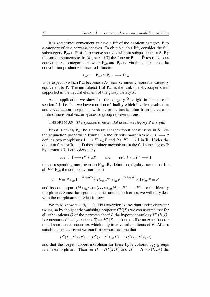
52 Chapter 3 – Perverse sheaves on semiabelian varieties
It is sometimes convenient to have a lift of the quotient category P toa category of true perverse sheaves. To obtain such a lift, consider the fullsubcategory Pint ⊂ P of all perverse sheaves without subquotients in S. Bythe same arguments as in [41, sect. 3.7] the functor P −→ P restricts to anequivalence of categories between Pint and P, and via this equivalence theconvolution product ∗ induces a bifunctor
∗int : Pint×Pint −→ Pint
with respect to which Pint becomes a Λ-linear symmetric monoidal categoryequivalent to P. The unit object 1 of Pint is the rank one skyscraper sheafsupported in the neutral element of the group variety X .
As an application we show that the category P is rigid in the sense ofsection 2.1, i.e. that we have a notion of duality which involves evaluationand coevaluation morphisms with the properties familiar from the case offinite-dimensional vector spaces or group representations.
THEOREM 3.9. The symmetric monoidal abelian category P is rigid.
Proof. Let P ∈ Pint be a perverse sheaf without constituents in S. Viathe adjunction property in lemma 3.4 the identity morphism idP : P −→ Pdefines two morphisms 1 −→ P∨ ∗∗ P and P ∗! P∨ −→ 1 in D. Under thequotient functor D−→D these induce morphisms in the full subcategory Pby lemma 3.7. Let us denote by
coev : 1−→ P∨ ∗int P and ev : P∗int P∨ −→ 1
the corresponding morphisms in Pint. By definition, rigidity means that forall P ∈ Pint the composite morphism
γ : P = P∗int 1id∗int coev // P∗int P∨ ∗int P
ev∗int id // 1∗int P = P
and its counterpart (id∗int ev) (coev∗int id) : P∨ −→ P∨ are the identitymorphisms. Since the argument is the same in both cases, we will only dealwith the morphism γ in what follows.
We must show γ − idP = 0. This assertion is invariant under charactertwists, so by the generic vanishing property GV (X) we can assume that forall subquotients Q of the perverse sheaf P the hypercohomology H•(X ,Q)is concentrated in degree zero. Then H•(X ,−) behaves like an exact functoron all short exact sequences which only involve subquotients of P. After asuitable character twist we can furthermore assume that
H•(X ,P∨ ∗! P) = H•(X ,P∨ ∗int P) = H•(X ,P∨ ∗∗P)
and that the forget support morphism for these hypercohomology groupsis an isomorphism. Then for H = H•(X ,P) and H∨ = HomΛ(H,Λ) the
3.4. Tannakian categories 53
diagrams in [41, appendix A.5.4] show that the morphism
Λ = H•(X ,1)coev∗ // H•(X ,P∨ ∗int P) = H•(X ,P∨ ∗∗P) = H∨⊗Λ H
is the coevaluation in the category of vector spaces, and dually for ev. Sincethe category of vector spaces of finite dimension over Λ is rigid, it followsthat on hypercohomology γ− idP induces the zero morphism. Accordinglythe perverse subquotient Q = P/ker(γ − idP) of P has H•(X ,Q) = 0. Bydefinition of Pint it follows that Q = 0 and hence that γ− idP = 0.
This in particular allows to define the Tannaka groups we are interestedin, generalizing those in corollary 2.14. For P ∈ P we denote by 〈P〉 ⊂ Pthe full subcategory of all objects which are isomorphic to subquotients ofconvolution powers of P⊕P∨. Recall that full subcategories of this formare said to be finitely tensor generated. By construction they inherit from Pthe structure of a rigid symmetric monoidal Λ-linear abelian category, andwe claim that they are neutral Tannakian in the following sense.
COROLLARY 3.10. For every P ∈ P there exists an affine algebraicgroup G = G(P) over Λ and an equivalence
ω : 〈P〉 ∼−→ RepΛ(G)
with the rigid symmetric monoidal Λ-linear abelian category RepΛ(G) offinite-dimensional algebraic representations of G.
Proof. Consider P as an object of the lifted category Pint ⊂ P. Bytheorem 3.1 there exists a character χ ∈ Π(X) such that all constituentsof all convolution powers
(P⊕P∨)χ ∗int · · · ∗int (P⊕P∨)χ
have their hypercohomology concentrated in degree zero (indeed these arecountably many conditions, and identifying Π(X)l as in [41, sect. 3.2] withthe set of Λ-valued points of the affine scheme Spec(Λ⊗Zl Zl[[t1, . . . , tn]])for some n> 0 one checks that Π(X)l cannot be covered by countably manyproper closed subsets — for this one may proceed by induction on n, usingthe description of ideals given in proposition A.2.2.3 of loc. cit.). For sucha character χ the functor Q 7→ H0(X ,Qχ) is a fibre functor from 〈P〉 tothe category of finite-dimensional vector spaces, and our corollary followsfrom theorem 3.9 via the Tannakian formalism [33, th. 2.11].
The above fibre functor depends on the chosen character twist (thoughall choices lead to isomorphic Tannaka groups), and this is the reason whywe have restricted ourselves to finitely tensor generated subcategories. Fora more canonical construction one may as in [41, th. 3.7.5] take the functorwhich to a perverse sheaf assigns the generic fibre of its Mellin transform,
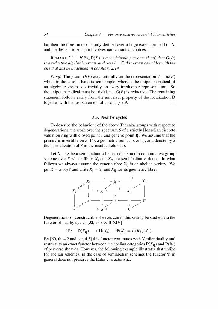
54 Chapter 3 – Perverse sheaves on semiabelian varieties
but then the fibre functor is only defined over a large extension field of Λ,and the descent to Λ again involves non-canonical choices.
REMARK 3.11. If P ∈ P(X) is a semisimple perverse sheaf, then G(P)is a reductive algebraic group, and over k =C this group coincides with theone that has been defined in corollary 2.14.
Proof. The group G(P) acts faithfully on the representation V = ω(P)which in the case at hand is semisimple, whereas the unipotent radical ofan algebraic group acts trivially on every irreducible representation. Sothe unipotent radical must be trivial, i.e. G(P) is reductive. The remainingstatement follows easily from the universal property of the localization Dtogether with the last statement of corollary 2.9.
3.5. Nearby cycles
To describe the behaviour of the above Tannaka groups with respect todegenerations, we work over the spectrum S of a strictly Henselian discretevaluation ring with closed point s and generic point η . We assume that theprime l is invertible on S. Fix a geometric point η over η , and denote by Sthe normalization of S in the residue field of η .
Let X → S be a semiabelian scheme, i.e. a smooth commutative groupscheme over S whose fibres Xs and Xη are semiabelian varieties. In whatfollows we always assume the generic fibre Xη is an abelian variety. Weput X = X×S S and write Xs = Xs and Xη for its geometric fibres.
Xsi //
uuuuu
uuuuu
Xvvv
vvXη
joo
yysssss
Xs
i //
X
Xη
joo
sssssssssssss
// Szzttttt
oo η
xxrrrrrr
s // S ηoo
Degenerations of constructible sheaves can in this setting be studied via thefunctor of nearby cycles [32, exp. XIII-XIV]
Ψ : D(Xη) −→ D(Xs), Ψ(K) = i∗(R j∗(K)).
By [60, th. 4.2 and cor. 4.5] this functor commutes with Verdier duality andrestricts to an exact functor between the abelian categories P(Xη) and P(Xs)of perverse sheaves. However, the following example illustrates that unlikefor abelian schemes, in the case of semiabelian schemes the functor Ψ ingeneral does not preserve the Euler characteristic.
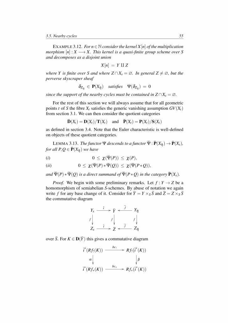
3.5. Nearby cycles 55
EXAMPLE 3.12. For n∈N consider the kernel X [n] of the multiplicationmorphism [n] : X −→ X. This kernel is a quasi-finite group scheme over Sand decomposes as a disjoint union
X [n] = Y q Z
where Y is finite over S and where Z ∩Xs = ∅. In general Z 6= ∅, but theperverse skyscraper sheaf
δZη∈ P(Xη) satisfies Ψ(δZη
) = 0
since the support of the nearby cycles must be contained in Z∩Xs =∅.
For the rest of this section we will always assume that for all geometricpoints t of S the fibre Xt satisfies the generic vanishing assumption GV (Xt)from section 3.1. We can then consider the quotient categories
D(Xt) = D(Xt)/T(Xt) and P(Xt) = P(Xt)/S(Xt)
as defined in section 3.4. Note that the Euler characteristic is well-definedon objects of these quotient categories.
LEMMA 3.13. The functor Ψ descends to a functor Ψ : P(Xη)→ P(Xs),for all P,Q ∈ P(Xη) we have
0 ≤ χ(Ψ(P)) ≤ χ(P),(i)
0 ≤ χ(Ψ(P)∗Ψ(Q)) ≤ χ(Ψ(P∗Q)),(ii)
and Ψ(P)∗Ψ(Q) is a direct summand of Ψ(P∗Q) in the category P(Xs).
Proof. We begin with some preliminary remarks. Let f : Y → Z be ahomomorphism of semiabelian S-schemes. By abuse of notation we againwrite f for any base change of it. Consider for Y = Y ×S S and Z = Z×S Sthe commutative diagram
Ysi //
f
Y
f
Yη
joo
f
Zsi // Z Zη
joo
over S. For K ∈ D(Y ) this gives a commutative diagram
i∗(R f!(K))bc! //
α
R f!(i∗(K))
β
i∗(R f∗(K))bc∗ // R f∗(i
∗(K))
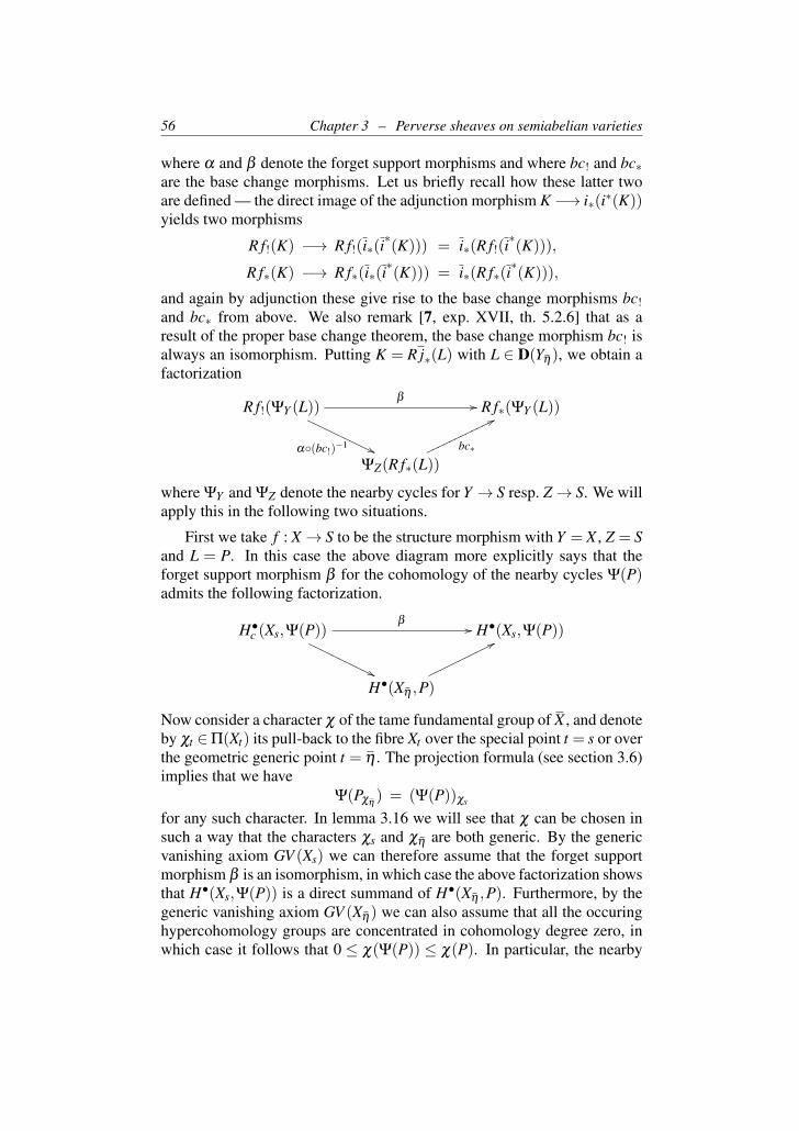
56 Chapter 3 – Perverse sheaves on semiabelian varieties
where α and β denote the forget support morphisms and where bc! and bc∗are the base change morphisms. Let us briefly recall how these latter twoare defined — the direct image of the adjunction morphism K −→ i∗(i∗(K))yields two morphisms
R f!(K) −→ R f!(i∗(i∗(K))) = i∗(R f!(i
∗(K))),
R f∗(K) −→ R f∗(i∗(i∗(K))) = i∗(R f∗(i
∗(K))),
and again by adjunction these give rise to the base change morphisms bc!and bc∗ from above. We also remark [7, exp. XVII, th. 5.2.6] that as aresult of the proper base change theorem, the base change morphism bc! isalways an isomorphism. Putting K = R j∗(L) with L ∈ D(Yη), we obtain afactorization
R f!(ΨY (L))β
//
α(bc!)−1 ''PPPPPPPPPPP
R f∗(ΨY (L))
ΨZ(R f∗(L))bc∗
77nnnnnnnnnnnn
where ΨY and ΨZ denote the nearby cycles for Y → S resp. Z→ S. We willapply this in the following two situations.
First we take f : X → S to be the structure morphism with Y = X , Z = Sand L = P. In this case the above diagram more explicitly says that theforget support morphism β for the cohomology of the nearby cycles Ψ(P)admits the following factorization.
H•c (Xs,Ψ(P))β
//
''OOOOOOOOOOOH•(Xs,Ψ(P))
H•(Xη ,P)
77ooooooooooo
Now consider a character χ of the tame fundamental group of X , and denoteby χt ∈Π(Xt) its pull-back to the fibre Xt over the special point t = s or overthe geometric generic point t = η . The projection formula (see section 3.6)implies that we have
Ψ(Pχη) = (Ψ(P))χs
for any such character. In lemma 3.16 we will see that χ can be chosen insuch a way that the characters χs and χη are both generic. By the genericvanishing axiom GV (Xs) we can therefore assume that the forget supportmorphism β is an isomorphism, in which case the above factorization showsthat H•(Xs,Ψ(P)) is a direct summand of H•(Xη ,P). Furthermore, by thegeneric vanishing axiom GV (Xη) we can also assume that all the occuringhypercohomology groups are concentrated in cohomology degree zero, inwhich case it follows that 0 ≤ χ(Ψ(P)) ≤ χ(P). In particular, the nearby
3.5. Nearby cycles 57
cycles functor Ψ then sends the Serre subcategory S(Xη)⊂ P(Xη) into theSerre subcategory S(Xs)⊂ P(Xs) and hence induces a functor
Ψ : P(Xη)−→ P(Xs)
between the quotient categories. The property (i) of Ψ is inherited from thecorresponding estimate for Ψ shown above.
Secondly we take f = m to be the group law, with Y = X ×k X , Z = Xand L = PQ. In D(Xs) we can identify ΨZ(R f∗(L)) with Ψ(P∗Q). Sinceby [60, th. 4.7] the exterior tensor product commutes with nearby cycles,we can also identify R f∗(ΨY (L)) with Ψ(P)∗Ψ(Q). Then the factorizationof β from above shows that the nearby cycles Ψ(P∗Q) admit Ψ(P)∗Ψ(Q)as a direct summand in P(Xs). Hence (ii) follows.
In general we cannot expect Ψ to be a tensor functor since it does notpreserve the Euler characteristic (see example 3.12). In what follows wewill call a perverse sheaf P on Xη admissible if
χ(Ψ(P)) = χ(P).
Note that for an abelian scheme X → S every perverse sheaf is admissiblesince the nearby cycles are compatible with proper morphisms.
LEMMA 3.14. The admissible objects form a rigid symmetric monoidalfull abelian subcategory
P(Xη)ad ⊂ P(Xη)
which is stable under the formation of extensions and subquotients.
Proof. Any short exact sequence 0→ P1 → P2 → P3 → 0 in P(Xη) ismapped under the nearby cycles functor to a short exact sequence in thecategory P(Xs). Then in particular
χ(P2) = χ(P1)+χ(P3) and χ(Ψ(P2)) = χ(Ψ(P1))+χ(Ψ(P3))
because the Euler characteristic is additive in short exact sequences. But onthe other hand χ(Pi)≥ χ(Ψ(Pi)) for i = 1,2,3 by lemma 3.13 (i). Hence itfollows that
χ(Pi) = χ(Ψ(Pi)) holds for i = 2 iff it holds for i = 1 and i = 3.
In other words, the perverse sheaf P2 is admissible if and only if both P1and P3 are admissible. So the category of admissible objects is stable underthe formation of extensions and subquotients.
58 Chapter 3 – Perverse sheaves on semiabelian varieties
It remains to show that for admissible P1,P2 ∈ P(Xη) also P1 ∗ P2 isadmissible. This follows from
χ(P1 ∗P2) = χ(P1) ·χ(P2) (part (d) of lemma 3)
= χ(Ψ(P1)) ·χ(Ψ(P2)) (admissibility of P1, P2)
= χ(Ψ(P1)∗Ψ(P2)) (part (d) of lemma 3)
≤ χ(Ψ(P1 ∗P2)) (part (ii) of lemma 12)
≤ χ(P1 ∗P2) (part (i) of lemma 12)
which implies that the last two estimates must in fact be equalities.
Concerning the failure of tensor functoriality it now follows that thesituation is as good as one could possibly hope for.
THEOREM 3.15. On the rigid symmetric monoidal abelian subcategoryof admissible objects, the nearby cycles define a tensor functor ACU
Ψ : P(Xη)ad −→ P(Xs)
so that for P ∈ Padη we obtain a closed immersion G(Ψ(P)) → G(P).
Proof. Let P1,P2 ∈ P(Xη)ad . The last statement in lemma 3.13 (ii) gives
a split monomorphism
Ψ(P1)∗Ψ(P2) → Ψ(P1 ∗P2)
in the abelian category P(Xs). But χ(Ψ(P1)∗Ψ(P2)) = χ(Ψ(P1 ∗P2)) as wehave seen in the proof of lemma 3.14. So the above monomorphism is anisomorphism in P(Xs), and hence Ψ is a tensor functor on P(Xη)
ad . For thestatement about the Tannaka groups, recall that by definition every objectof 〈Ψ(P)〉 is a subquotient of the image under Ψ of some object in 〈P〉. Soour claim follows from the Tannakian formalism [33, prop. 2.21b)].
3.6. Specialization of characters
Let X −→ S be a semiabelian scheme as above. Since we assumed theprime number l to be invertible on S, we know from [17] that the (tame)pro-l fundamental groups
π1(Xη ,0)l = πt1(Xη ,0)l and π1(Xs,0)l = π
t1(Xs,0)l
are free Zl-modules of finite rank. However, the basic example of abelianvarieties with semiabelian reduction illustrates that in general π1(Xs,0)lwill have strictly smaller rank than π1(Xη ,0). To complete the proof oflemma 3.13 we thus need to justify why in passing from the generic to thespecial fibre, we retain enough characters to apply the generic vanishingassumption from section 3.1 on both fibres. To this end, let Π(X)l denotethe group of all continuous characters of π1(X ,x)l for any chosen geometric
3.6. Specialization of characters 59
point x in X . The passage to a different choice of x corresponds to an innerautomorphism of the fundamental group, which is not seen on the level ofcharacters. So we have well-defined restriction homomorphisms
i∗ : Π(X)l −→ Π(Xs)l, χ 7→ χs,
j∗ : Π(X)l −→ Π(Xη)l, χ 7→ χη .
Any character χ ∈Π(X)l defines a local system Lχ on X , and for K ∈D(X)the projection formula shows that
Ψ(Kχη) = i∗(R j∗(K⊗Λ j∗(Lχ))) = i∗(R j∗(K)⊗Λ Lχ) = Ψ(K)χs.
To apply this formula in relation with the vanishing axiom from section 3.1,one can use the following well-known result.
LEMMA 3.16. The pull-back homomorphisms i∗ and j∗ on charactersare an epimorphism resp. an isomorphism
Π(Xs)l Π(X)loooo ∼ // Π(Xη)l.
In particular, for all open dense subsets Us ⊆Π(Xs)l and Uη ⊆Π(Xη)l onecan find χ ∈Π(X)l such that
χs ∈ Us and χη ∈ Uη .
Proof. Choose any path from the point 0 in Xs to the point x in X . Wefirst claim that the corresponding homomorphism
i∗ : π1(Xs,0)l −→ π1(X ,x)l
is injective. To check this, we must by the criterion in [51, exp. V, cor. 6.8]show that every finite etale cover
f : Y −→ Xs
of l-primary degree is dominated by a connected component Z0s ⊆ Zs of the
special fibre Zs of some finite etale cover h : Z −→ X of l-primary degree asindicated in the following diagram.
Z0s
// Zs // Z
h
Y
f
Xs // X
We can assume that Y is connected and that f is a Galois cover. Sincethe prime l is invertible on S, it then follows that Y can be made into asemiabelian variety such that f is an isogeny [17]. So by [15, th. 7.3.5]
60 Chapter 3 – Perverse sheaves on semiabelian varieties
there exists an isogeny g : Xs −→ Y such that g f and hence also f g isthe multiplication by n = lν for some ν . Thus it suffices to treat the casewhere Y = Xs and where f = [n] : Xs −→ Xs is the multiplication by n.
If we were dealing with an abelian scheme, we could now take Z = Xand define h = [n] : X −→ X to be the multiplication by n. However, for asemiabelian scheme the multiplication by n is in general not a finite etalecover. To get around this problem we consider the Neron model of thegeneric fibre Xη , which will allow to find a finite etale cover h : Z −→ Xwhose base change under S −→ S gives the desired h. But before we cancarry out this idea, we need to perform a base change to make sure that theNeron model does what we want.
Note that X and the special fibre Xs do not change if we replace thegiven semiabelian scheme X −→ S by a base change X ′ = X ×S S′ −→ S′
where S′ denotes the normalization of S in a finite extension of the quotientfield κ(η). After such a base change we can assume that all n-torsion pointsof the generic fibre Xη are defined over κ(η). Then the universal propertyof the Neron model
N −→ Sof Xη implies that the multiplication morphism [n] : N −→ N has constantfibre degree over its image and thus restricts to a finite etale cover overthe image. This image contains the connected component N0 which byprop. 7.4.3 of loc. cit. is isomorphic to X . Hence if we define h : Z −→ Xvia the fibre product in the Cartesian diagram
Z
h
// N
[n]
X // N
then h will be a finite etale cover of X . The special fibre Zs will in generalnot be connected, but on the connected component
Z0s = Zs∩N0
s = N0s = Xs
the cover h restricts to the multiplication morphism f = [n] : Xs −→ Xs. Sowe can put Z = Z×S S and take h to be the base change of h.
Summing up, this shows that the homomorphism i∗ : π1(Xs)l −→ π1(X)lis an embedding. With the same arguments as above one also checks thatthe homomorphism j∗ : π1(Xη)l −→ π1(X)l is an isomorphism (surjectivityis in this case clear because a finite etale cover of X is connected iff itrestricts to a connected cover of Xη ). From this one deduces that the inducedhomomorphisms
Π(X)l −→ Π(Xs)l and Π(X)l −→ Π(Xη)l
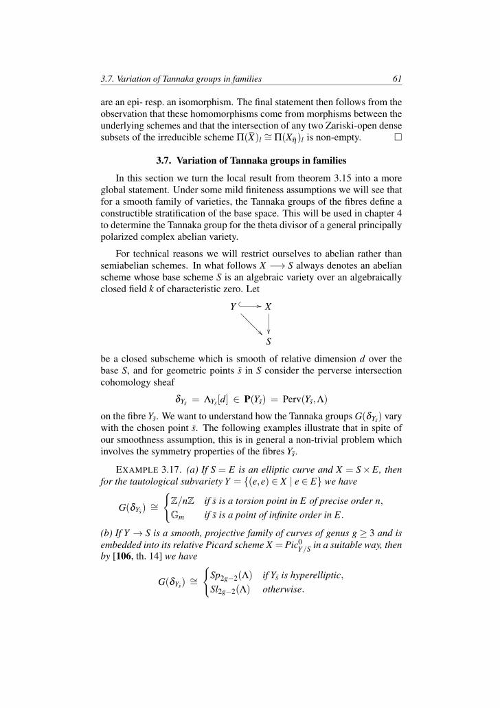
3.7. Variation of Tannaka groups in families 61
are an epi- resp. an isomorphism. The final statement then follows from theobservation that these homomorphisms come from morphisms between theunderlying schemes and that the intersection of any two Zariski-open densesubsets of the irreducible scheme Π(X)l
∼= Π(Xη)l is non-empty.
3.7. Variation of Tannaka groups in families
In this section we turn the local result from theorem 3.15 into a moreglobal statement. Under some mild finiteness assumptions we will see thatfor a smooth family of varieties, the Tannaka groups of the fibres define aconstructible stratification of the base space. This will be used in chapter 4to determine the Tannaka group for the theta divisor of a general principallypolarized complex abelian variety.
For technical reasons we will restrict ourselves to abelian rather thansemiabelian schemes. In what follows X −→ S always denotes an abelianscheme whose base scheme S is an algebraic variety over an algebraicallyclosed field k of characteristic zero. Let
Y //
???
????
? X
S
be a closed subscheme which is smooth of relative dimension d over thebase S, and for geometric points s in S consider the perverse intersectioncohomology sheaf
δYs = ΛYs[d] ∈ P(Ys) = Perv(Ys,Λ)
on the fibre Ys. We want to understand how the Tannaka groups G(δYs) varywith the chosen point s. The following examples illustrate that in spite ofour smoothness assumption, this is in general a non-trivial problem whichinvolves the symmetry properties of the fibres Ys.
EXAMPLE 3.17. (a) If S = E is an elliptic curve and X = S×E, thenfor the tautological subvariety Y = (e,e) ∈ X | e ∈ E we have
G(δYs)∼=
Z/nZ if s is a torsion point in E of precise order n,Gm if s is a point of infinite order in E.
(b) If Y → S is a smooth, projective family of curves of genus g ≥ 3 and isembedded into its relative Picard scheme X = Pic0
Y/S in a suitable way, thenby [106, th. 14] we have
G(δYs)∼=
Sp2g−2(Λ) if Ys is hyperelliptic,Sl2g−2(Λ) otherwise.
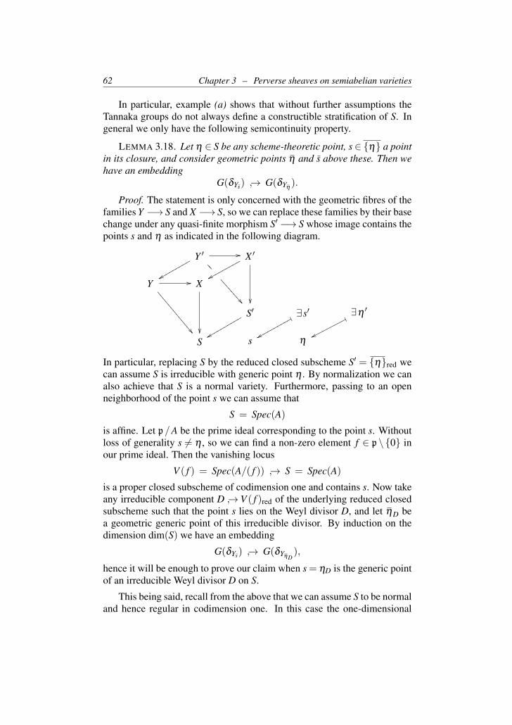
62 Chapter 3 – Perverse sheaves on semiabelian varieties
In particular, example (a) shows that without further assumptions theTannaka groups do not always define a constructible stratification of S. Ingeneral we only have the following semicontinuity property.
LEMMA 3.18. Let η ∈ S be any scheme-theoretic point, s∈ η a pointin its closure, and consider geometric points η and s above these. Then wehave an embedding
G(δYs) → G(δYη).
Proof. The statement is only concerned with the geometric fibres of thefamilies Y −→ S and X −→ S, so we can replace these families by their basechange under any quasi-finite morphism S′ −→ S whose image contains thepoints s and η as indicated in the following diagram.
Y ′ //
xxqqqqqqqqq ;;
;;;
;;;;
;
X ′
xxqqqqqqqqq
Y //
:::
::::
::::
::X
S′
xxrrrrrrrrrr ∃s′1
xxqqqqqqqqqq∃η ′0
wwppppppppp
S s η
In particular, replacing S by the reduced closed subscheme S′ = ηred wecan assume S is irreducible with generic point η . By normalization we canalso achieve that S is a normal variety. Furthermore, passing to an openneighborhood of the point s we can assume that
S = Spec(A)
is affine. Let p/A be the prime ideal corresponding to the point s. Withoutloss of generality s 6= η , so we can find a non-zero element f ∈ p \ 0 inour prime ideal. Then the vanishing locus
V ( f ) = Spec(A/( f )) → S = Spec(A)
is a proper closed subscheme of codimension one and contains s. Now takeany irreducible component D → V ( f )red of the underlying reduced closedsubscheme such that the point s lies on the Weyl divisor D, and let ηD bea geometric generic point of this irreducible divisor. By induction on thedimension dim(S) we have an embedding
G(δYs) → G(δYηD),
hence it will be enough to prove our claim when s = ηD is the generic pointof an irreducible Weyl divisor D on S.
This being said, recall from the above that we can assume S to be normaland hence regular in codimension one. In this case the one-dimensional
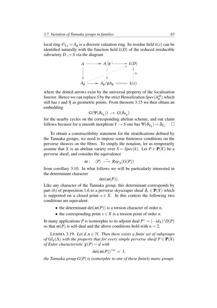
3.7. Variation of Tannaka groups in families 63
local ring OS,s = Ap is a discrete valuation ring. Its residue field k(s) can beidentified naturally with the function field k(D) of the reduced irreduciblesubvariety D → S via the diagram
A // //
A/p //
k(D)
Ap
55
// // Ap/pAp k(s)
∼=
OO
where the dotted arrows exist by the universal property of the localizationfunctor. Hence we can replace S by the strict Henselization Spec(Ash
p ) whichstill has s and η as geometric points. From theorem 3.15 we then obtain anembedding
G(Ψ(δYη)) → G(δYη
)
for the nearby cycles on the corresponding abelian scheme, and our claimfollows because for a smooth morphism Y → S one has Ψ(δYη
) = δYs .
To obtain a constructibility statement for the stratifications defined bythe Tannaka groups, we need to impose some finiteness conditions on theperverse sheaves on the fibres. To simply the notation, let us temporarilyassume that X is an abelian variety over S = Spec(k). Let P ∈ P(X) be aperverse sheaf, and consider the equivalence
ω : 〈P〉 ∼−→ RepΛ(G(P))
from corollary 3.10. In what follows we will be particularly interested inthe determinant character
det(ω(P)).Like any character of the Tannaka group, this determinant corresponds bypart (b) of proposition 1.6 to a perverse skyscraper sheaf δx ∈ P(X) whichis supported on a closed point x ∈ X . In this context the following twoconditions are equivalent:
• the determinant det(ω(P)) is a torsion character of order n,• the corresponding point x ∈ X is a torsion point of order n.
In many applications P is isomorphic to its adjoint dual P∨ = (−idX)∗D(P)
so that ω(P) is self-dual and the above conditions hold with n = 2.
LEMMA 3.19. Let d,n ∈ N. Then there exists a finite set of subgroupsof Gld(Λ) with the property that for every simple perverse sheaf P ∈ P(X)of Euler characteristic χ(P) = d with
det(ω(P))⊗n = 1,
the Tannaka group G(P) is isomorphic to one of these finitely many groups.
64 Chapter 3 – Perverse sheaves on semiabelian varieties
Proof. Lemma B.1 and B.2 in the appendix show that up to conjugationthere are only finitely many possibilities for the Tannaka group G = G(P)as a subgroup of Gld(Λ).
Let us now return to the case of an abelian scheme p : X −→ S whosebase scheme is an arbitrary variety S over the algebraically closed field kof characteristic zero. For any sheaf complex P ∈ D(X) and any geometricpoint s of S we will denote by
Ps = i∗s (P) ∈ D(Xs)
the restriction to the geometric fibre is : Xs −→ X . Then the constructibilityresult we are interested in can be formulated as follows.
PROPOSITION 3.20. Let n ∈N, and consider a complex P ∈D(X) suchthat for each geometric point s of S, the restriction Ps is a simple perversesheaf with
det(ω(Ps))⊗n = 1.
Then there are reductive algebraic groups G1, . . . ,Gm and a stratificationinto locally closed subsets
S =m⊔
i=0
Si such that G(Ps) = Gi for all geometric points s in Si.
Proof. Recall from [29, prop. 3.1(c)] that if V is a finite-dimensionalvector space over Λ, then any reductive algebraic subgroup of Gl(V ) isdetermined uniquely by its subspaces of invariants in the tensor powers W⊗r
of W = V ⊕V∨ with r ∈ N. Furthermore, if we only want to distinguishbetween finitely many given reductive subgroups up to conjugacy, then itsuffices to look at exponents r ≤ r0 for some fixed r0 ∈ N.
Hence in view of lemma 3.19 our claim will follow if we can show thatin a suitable sense, the tensor functor ω : 〈Ps〉 −→ RepΛ(G(Ps)) in the proofof corollary 3.10 varies in a constructible way with the geometric point sand that the subspaces of invariants — corresponding to the direct sum ofall direct summands 1 = δ0 in the convolution powers of Ps⊕P∨s — alsovary in a constructible way. More precisely, we would be done if we couldshow that there exist
(a) a complex P∨ ∈ D(X) which on each geometric fibre Xs restrictsto the adjoint dual
P∨s = (−id)∗D(Ps),
(b) a character χ ∈Π(X) such that for the twist Q = Pχ⊕P∨χ the directimage complex
W = Rp∗(Q)
3.7. Variation of Tannaka groups in families 65
is a constructible sheaf on S which is concentrated in degree zeroand has geometric stalks
Ws = H0(Xs,Qs) = ω(Ps⊕P∨s ),
(c) for each r≤ r0 a constructible subsheaf of W ⊗r whose stalks at anygeometric point s coincide under the above identification with thecohomology of the direct sum of all skyscraper summands 1 = δ0in the convolution Q∗rs = Qs ∗ · · · ∗Qs.
In general this is too much to expect. However, since the groups Gs = G(Ps)only depend on the geometric fibres of our abelian scheme and since forthe proof of constructibility we can argue by Noetherian induction on thedimension dim(S), it will do no harm if we replace our original abelianscheme by the base change
X ′ = X×S S′ −→ S′
under a quasi-finite etale morphism S′ −→ S and also replace P ∈ D(X)by its pull-back P′ ∈ D(X ′). In particular, for the proof of the propositionwe are free to replace our base scheme S by arbitrary Zariski-open densesubsets of S and also by finite etale covers of such subsets.
With this extra freedom, property (a) can be obtained from the generalfact [64, prop. 1.1.7] that for any morphism p : X → S of varieties withsmooth target variety S and any P ∈ D(X), there is a Zariski-open densesubset S′ → S such that the formation of the relative dual
DX/S(P) = RH om(P, p!ΛS)
commutes with every base change that factors over S′ → S. Property (b) willbe obtained in lemma 3.21 after a base change to a finite etale cover of someZariski-open dense subset of S, which is needed to make sure that there aresufficiently many characters available. For part (c) consider the relativeconvolution power Q∗r = Ra∗(QS · · ·S Q) where a : X×S · · ·×S X −→ Xis the group law. We have a relative Kunneth isomorphism
Rp∗(Q∗r)∼=−→ (Rp∗(Q))⊗r = W ⊗r
as in the absolute case. Let Z ⊂ X be the zero section of our abelian scheme,and consider the morphism
ϕ : Rp∗(RH om(ΛZ,Q∗r)) −→ RH om(ΛS,W⊗r) ∼= W ⊗r
which corresponds by adjunction to the composite morphism ψ given bythe following diagram (where the diagonal arrow on the left comes from
66 Chapter 3 – Perverse sheaves on semiabelian varieties
the adjoint of the relative Kunneth isomorphism).
RH om(ΛZ,Q∗r)ψ
//
((QQQQQQQQQQQQQp!(RH om(ΛS,W
⊗r))
RH om(p∗(ΛS), p!(W ⊗r))
∼=
55kkkkkkkkkkkkkk
As a candidate for the constructible subsheaf in part (c) we take the image ofthe induced morphism H 0(ϕ) on the stalk cohomology sheaves in degreezero. After shrinking S we can by loc. cit. assume that the occuring RH omcommute with base change. If we put
K = (Ps⊕P∨s )∗r
and denote by χs the restriction of the character χ to the geometric fibre Xs,then on stalks we obtain a commutative diagram
H0(Xs,RH om(δ0,Kχs))H 0(ϕ)s // H0(Xs,Kχs)
⊕i∈ZExti(δ0,
pH−i(K)χs)// Hom(δ0,
pH0(K)χs)
OO
where the Ext and Hom in the lower row refer to the abelian category P(Xs)and where the vertical identifications come from Gabber’s decompositiontheorem by which Kχs
∼=⊕
i∈ZpH i(K)χs[−i]. The fact that H 0(ϕ)s factors
over the projection in the lower row follows from the observation that bypart (b) we have H•(Xs,
pH−i(K)χs) = 0 for all i 6= 0. Hence (c) follows aswell, and we are done.
In the above proof we have used that after a suitable quasi-finite etalebase change there exist enough characters χ ∈ Π(X) so that we can applythe vanishing theorem from section 3.1 fibre by fibre. More precisely wehave the following result.
LEMMA 3.21. Let P ∈D(X) be a complex which restricts to a perversesheaf on each geometric fibre of the abelian scheme X → S, and supposethat S is irreducible. Then there exists
• a quasi-finite etale morphism f : S′→ S,• a character χ ∈Π(X ′) for the abelian scheme X ′ = X×S S′,
such that the direct image of P′ = (idX , f )∗(P) ∈ D(X ′) under the structuremorphism p : X ′→ S′ satisfies
H i(Rp∗(P′⊗Λ Lχ)) = 0 for all i 6= 0.
3.7. Variation of Tannaka groups in families 67
Proof. Take a geometric generic point η of S. The set of all torsioncharacters χη : π1(Xη ,0) −→ Λ∗ is dense in the character torus Π(Xη), soby the generic vanishing theorem from chapter 1 we can find a character χη
of some finite order N ∈N with the property that H i(Xη ,Pη⊗Λ Lχη) = 0 for
all i 6= 0. If we could extend this character to a global character χ ∈Π(X),then the above vanishing property would mean that for the direct imageunder p : X → S the generic stalk cohomology satisfies
H i(Rp∗(P⊗Λ Lχ))η = 0 for all i 6= 0.
Since the cohomology sheaves are constructible, the vanishing of their stalksat the geometric generic point η would imply their vanishing over someopen dense subset U ⊆ S, and we would be done even without the need topass to a finite etale cover of the base variety S and without using that χη isa torsion character of order N.
However, in general it may be impossible to find χη ∈ Π(Xη) with therequired property which lifts to some χ ∈ Π(X) (for example, think of theuniversal abelian scheme X over a finite level cover S of the moduli space ofprincipally polarized abelian varieties — here the abelianized fundamentalgroup πab
1 (X) and hence also the group Π(X) is finite). To get around thisproblem we perform a base change under a finite etale cover depending onthe chosen torsion character χη . Consider the split exact fibration sequence
0 // π1(Xη ,0) // π1(X ,0) // π1(S,η) //xx
0
from [51, exp. XIII, prop. 4.3 and ex. 4.4], where the splitting comes fromthe zero section of our abelian scheme. Via the splitting, the group π1(S,η)acts by conjugation on π1(Xη ,0) and hence on the corresponding charactertorus Π(Xη). Since the group of torsion points of order N in this torusis finite, we can find a normal subgroup of finite index in π1(S,η) whichfixes every such torsion point. This normal subgroup defines a finite etalecover S′ −→ S for which the character χη ∈ Π(Xη) can be extended to acharacter χ ∈ Π(X ′). After a base change by this finite etale cover we canthen proceed as in the first part of the proof.

CHAPTER 4
The Tannaka group of the theta divisor
The geometric relevance of the constructions in the previous chaptersis illustrated by the following example. Let X be a principally polarizedabelian variety (ppav) of dimension g over the complex numbers. The givenpolarization determines an ample theta divisor Θ⊂ X up to a translation bya point in X(C). For us it will be most convenient to choose a translationsuch that the theta divisor is symmetric, i.e. stable under −idX . Then theperverse intersection cohomology sheaf
δΘ = ICΘ[g−1]
will be isomorphic to its adjoint dual as defined in section 2.1. With thisnormalization, consider the Tannaka group G(δΘ) which describes the rigidsymmetric monoidal abelian category generated by the convolution powersof δΘ as in corollary 2.14 or equivalently in corollary 3.10. This Tannakagroup is a new invariant of the ppav, a reductive complex algebraic groupwhich behaves in a very different and much more rigid way than classicalinvariants such as Mumford-Tate groups do.
For example, for the Jacobian variety X = JC of a smooth projectivecurve C it has been shown in [106, p. 124 and th. 14] that
G(δΘ) =
Sp2g−2(C)/εg−1 if C is hyperelliptic,Sl2g−2(C)/µg−1 otherwise,
where µg−1 ⊂ Sl2g−2(C) denotes the central subgroup of g− 1st roots ofunity in the special linear group and εg−1 = µg−1∩±1 is its intersectionwith the symplectic group. In a nutshell, this behaviour can be explainedas follows. For a suitable choice of the Abel-Jacobi embedding C → X onecan use Brill-Noether theory and arguments from representation theory toshow that the Tannaka group of the perverse sheaf δC ∈ Perv(X ,C) is
G(δC) =
Sp2g−2(C) if C is hyperelliptic,Sl2g−2(C) otherwise,
and that δC corresponds to the standard representation of this group. Sinceon a Jacobian variety X = JC the theta divisor Θ is birational to the g−1st
symmetric product of the curve C, one deduces that the perverse sheaf δΘ
corresponds on the Tannakian side to the g−1st fundamental representation
69
70 Chapter 4 – The Tannaka group of the theta divisor
of the group G(δC), and this implies that the Tannaka group G(δΘ) of thetheta divisor has the form given above.
The high fundamental representation in the above example is accountedfor by the particular symmetry of the theta divisor of Jacobian varieties, andin general it is reasonable to expect the Tannaka groups G(δΘ) to be muchlarger. One may speculate [110] whether among all ppav’s of dimension gonly Jacobian varieties have the above Tannaka groups — this would givea Tannakian answer for the Schottky problem to characterize the locus ofJacobian varieties in the moduli space
Ag = Hg/Sp2g(Z),
where Hg denotes the Siegel upper half space. More generally, one mayask for the stratification of Ag defined by the invariant G(δΘ).
In this context, let us say that a statement holds for a general ppav ofdimension g if it holds for every ppav in a Zariski-open dense subset ofthe moduli space Ag. For example, the theta divisor of a general ppav issmooth by the results of Andreotti and Mayer [4]. For the open stratumin the above-mentioned stratification of Ag we discuss in this chapter thefollowing conjecture which goes back to the preprint [67].
CONJECTURE 4.1. If X is a complex ppav of dimension g equipped witha smooth symmetric theta divisor Θ⊂ X, then
G(δΘ) =
SOg!(C) for g odd,Spg!(C) for g even,
and δΘ corresponds to the standard representation of this group.
Intuitively, this conjecture says that in marked contrast with the singularsituation for Jacobian varieties, for a smooth theta divisor Θ the Tannakagroup G(δΘ) should be as large as possible — see lemma 4.6 below. Letus take a look at some small examples to begin with. The case g = 1 isof course trivial. For g = 2 every ppav with a smooth theta divisor is theJacobian of a smooth hyperelliptic curve; then our conjecture holds by theresult of [106] quoted above. Similarly, for g = 3 every ppav with a smooththeta divisor is the Jacobian of a smooth non-hyperelliptic curve, and inthis case the conjecture holds since the second fundamental representationof Sl4(C)/µ2 corresponds to the standard representation of SO6(C) via theexceptional isomorphism between these two groups. So the first open caseof our conjecture occurs for g = 4. This is the first case where the realm ofJacobian varieties is left, hence also the first non-trivial case of the Schottkyproblem, and indeed we will see in corollary 4.4 below that in this case theinvariant G(δΘ) determines the locus of Jacobian varieties in A4.
4.1. The Schottky problem in genus 4 71
To avoid case distinctions, from now on we put G(g) = SOg!(C) if g isodd and G(g) = Spg!(C) if g is even. The main goal of this chapter is toprove the following weaker version of our conjecture, extending ideas thathave been used in dimension g = 4 in the earlier preprint [67].
THEOREM 4.2. For a general complex ppav X of dimension g with asymmetric theta divisor Θ one has
G(δΘ) = G(g),
and δΘ corresponds to the standard representation of this group.
As we have remarked above, this essentially means that for a generalppav the Tannaka group of the theta divisor is as large as possible — themain task will be to find sufficiently large lower bounds on this group. Bya constructibility argument it suffices to do this for the generic fibre of asuitable family of ppav’s over a smooth complex algebraic curve S. So wecan apply degeneration methods: By theorem 3.15 the Tannaka group of thegeneric fibre admits those of the perverse sheaves of nearby cycles on thespecial fibres as subquotients. With this in mind, we collect in section 4.3some general properties of the monodromy filtration that allow to controlthe nearby cycles in concrete geometric situations. The crucial part of ourargument is then given in section 4.4 where we consider three degenerationsof a generic ppav — in one of them the theta divisor becomes nodal, andin the other two the ppav degenerates into a product of ppav’s resp. into aJacobian variety. In each case the nearby cycles contain a large irreducibleconstituent that can be controlled geometrically, and this will reduce theproof of our theorem to arguments in representation theory to be workedout in section 4.5.
4.1. The Schottky problem in genus 4
Before we come to the proof of theorem 4.2, let us briefly discuss itsconnection with the Schottky problem. Recall that in dimension g ≥ 4 theAndreotti-Mayer locus Ng ⊂ Ag of ppav’s with a singular theta divisor isitself a divisor with precisely two irreducible components [26]. One of thecomponents is the locus θnull,g of all ppav’s with a vanishing theta null; theother component contains the closure Jg of the locus of Jacobian varietiesand for g = 4 is equal to it [8]. This being said, in dimension g = 4 we cansharpen the formulation of theorem 4.2 as follows.
THEOREM 4.3. For g = 4 the locus of all ppav’s with G(δΘ) 6= Sp24(C)is contained in a Zariski-closed subset of A4 whose divisorial componentsare precisely J4 and θnull,4.
72 Chapter 4 – The Tannaka group of the theta divisor
The proof of this will be given along with our proof of theorem 4.2,based on the observation that every divisor on A4 intersects the locus ofJacobian varieties — on the Tannakian side this information is encoded inpart (3) of proposition 4.12 below. Assuming the theorem, we recover thefollowing result of [67].
COROLLARY 4.4. For g = 4 the invariant G = G(δΘ) determines boththe Jacobian locus and the theta null locus
J4 ⊂ A4 and θnull,4 ⊂ A4.
Proof. Theorem 4.3 says that the closure of the locus of all ppav’s in A4with G 6= Sp24(C) is a proper Zariski-closed subset, with J4 and θnull,4 asits only divisorial components. By the result quoted at the beginning of thischapter, the group G is equal to Sl6(C)/µ3 for a general ppav in the Jacobianlocus J4. By way of contrast, for a general ppav in θnull,4 the degenerationargument in part (2) of proposition 4.12 below shows that the irreduciblerepresentation W ∈ RepC(G) corresponding to the simple perverse sheaf δΘ
has dimension dim(W ) = g!− 2 = 22. In particular, for such a ppav thegroup G is different from Sl6(C)/µ3 since by [3] the latter does not admitan irreducible representation of dimension 22.
In this context, we remark that the possible singularities of theta divisorsin dimension g = 4 can be described explicitly as follows. Let J4,hyp bethe closure of the locus of Jacobian varieties of hyperelliptic curves, anddenote by A4,dec ⊂ θnull,4 ∩J4 the locus of decomposable ppav’s. Thenthe following types of singularities occur.
LEMMA 4.5. a) For ppav’s in J4 \ (θnull,4 ∩J4) the theta divisorshave precisely two singularities, both ordinary double points. b) For ppav’sin θnull,4 \ (θnull,4∩J4) they have only one singularity, again an ordinarydouble point. c) On (θnull,4 ∩J4) \ (J4,hyp ∪A4,dec) they have only onesingular point, and there the Hesse matrix of the Riemann theta functionhas rank three. d) On J4,hyp \ (J4,hyp∩A4,dec) the singular locus of eachtheta divisor has dimension one. e) On A4,dec it has dimension two.
Proof. It has been shown in [54, thm. 10 and cor. 15] that for a), b)and c) the rank of the Hesse matrix at any singular point of the theta divisoris the given one. In particular, in cases a) and b) only isolated singularitiesoccur. This also holds for c) since by Riemann’s singularity theorem thesingular locus of the theta divisor on a Jacobian variety is the Brill-Noethersubvariety W 1
g−1, which in the non-hyperelliptic case has dimension g−4 byMartens’ theorem [6, th. 4.5.1]. The number of singularities can be obtainedfrom [20, sect. 10] and from [8] and [81, case b2, p. 55f]. Part d) followsagain from Martens’ theorem, and e) is trivial.
4.2. Nondegenerate bilinear forms 73
4.2. Nondegenerate bilinear forms
In the introduction to this chapter we have remarked that conjecture 4.1essentially says that for a smooth theta divisor the associated Tannaka groupis as large as possible. To justify this interpretation, let X be a complex ppavof dimension g≥ 2 and Θ⊂ X a symmetric theta divisor. For simplicity weassume that the ppav X is indecomposable, in which case Θ is irreducibleand hence in particular normal by [36].
Then δΘ is a simple perverse sheaf, and by symmetry of the theta divisorit is isomorphic to its adjoint dual (δΘ)
∨ = (−id)∗D(δΘ). On the Tannakianside, if we denote by
ω : 〈δΘ〉∼−→ RepC(G(δΘ))
the tensor functor in corollary 3.10, then it follows that V = ω(δΘ) is anirreducible self-dual representation of G(δΘ). Any representation with theseproperties is either orthogonal or symplectic, depending on whether the unitobject 1 = δ0 of our Tannakian category lies in the alternating square Λ2(V )or in the symmetric square S2(V ). To decide which of the two possibilitiesoccurs, consider the commutativity constraint
S = SδΘ,δΘ: δΘ ∗δΘ
∼−→ δΘ ∗δΘ
as defined in section 2.1. We claim that this constraint S acts by (−1)g−1
on the stalk cohomology group H 0(δΘ ∗ δΘ)0 at the origin. Indeed wehave δΘ = ICΘ[g− 1], so our claim amounts to the statement that S actstrivially on the stalk cohomology group H 2g−2(ICΘ ∗ ICΘ)0. For this latterstatement one can use that since by assumption the theta divisor is normal,we have a natural identification
H 2g−2(ICΘ ∗ ICΘ)0 ∼= H 2g−2(CΘ ∗CΘ)0
which allows to replace the intersection cohomology sheaf with the constantsheaf. Then our claim easily follows via base change.
For the representation V = ω(δΘ) it follows from the above that theunit object 1 lies in the alternating square Λ2(V ) if g is even, resp. in thesymmetric square S2(V ) if g is odd. This implies
LEMMA 4.6. If the theta divisor Θ ⊂ X is smooth, then there exists anembedding
G(δΘ) → G(g) =
Spg!(C) for even gSOg!(C) for odd g
such that ω(δΘ) is the restriction of the standard representation of G(g).
74 Chapter 4 – The Tannaka group of the theta divisor
Proof. Since Θ is smooth, the irreducible representation V = ω(δΘ) isof dimension dimC(V ) = χ(δΘ) = g! by the Gauss-Bonnet formula, and wehave noted above that V is a symplectic resp. orthogonal representation if gis even resp. odd. This proves the lemma with the full orthogonal group inplace of the special orthogonal group. It remains to show that det(V ) is thetrivial character of G(δΘ). If not, the character det(V ) would by part (b) ofproposition 1.6 correspond to a skyscraper sheaf δx supported in a 2-torsionpoint x∈X(C)\0. For monodromy reasons it is impossible to select sucha 2-torsion point naturally on every ppav on an Zariski-open dense subsetof the moduli space Ag. So we can finish the proof by a specializationargument, using that the Tannaka group defines a constructible stratificationof the moduli space (see the remarks preceding proposition 4.12 below) andthat by theorem 3.15 it only becomes smaller on closed subsets.
4.3. Local monodromy
To find sufficiently large lower bounds on the Tannaka group of the thetadivisor on a general ppav, we will study degenerations of ppav’s in terms ofthe nearby cycles functor. For this purpose we gather in the present sectionsome general facts about the monodromy filtration that allow to get hold onthe nearby cycles in concrete geometric situations. Throughout we work inthe following algebraic setting.
Let S be the spectrum of a strictly Henselian discrete valuation ring (inour applications in proposition 4.12 it will be the strict Henselization of asmooth complex algebraic curve in the moduli space of ppav’s). We denoteby s the unique closed point of S and fix a geometric point η above thegeneric point η of S. For a separated S-scheme of finite type
f : Y −→ S
we consider as in section 3.5 the functor of nearby cycles
Ψ : P(Yη) = Perv(Yη ,Λ) −→ P(Ys) = Perv(Ys,Λ)
on perverse sheaves with coefficients in Λ = Ql for some fixed prime lwhich is invertible on S. Here we consider perverse sheaves on Xη andnot just perverse sheaves on the geometric fibre Xη since we want to keeptrack of the monodromy operation. By construction [32, exp. XIII], for anyperverse sheaf δ ∈ P(Yη) the local monodromy group G = Gal(η/η) actsnaturally on the nearby cycles Ψ(δ ) ∈ P(Ys). Since we are working over astrictly Henselian base, this group coincides with the inertia group.
If p ≥ 0 denotes the residue characteristic of the point s, the inertiagroup sits in an exact sequence 1→ P→ G→∏l′ 6=pZl′(1)→ 1 where thepro-p-group P is the wild inertia group and where l′ runs through the set
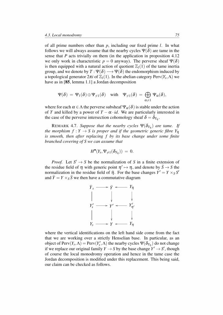
4.3. Local monodromy 75
of all prime numbers other than p, including our fixed prime l. In whatfollows we will always assume that the nearby cycles Ψ(δ ) are tame in thesense that P acts trivially on them (in the application in proposition 4.12we only work in characteristic p = 0 anyway). The perverse sheaf Ψ(δ )is then equipped with a natural action of quotient Zl(1) of the tame inertiagroup, and we denote by T : Ψ(δ )−→Ψ(δ ) the endomorphism induced bya topological generator 2πi of Zl(1). In the abelian category Perv(Ys,Λ) wehave as in [85, lemma 1.1] a Jordan decomposition
Ψ(δ ) = Ψ1(δ )⊕Ψ6=1(δ ) with Ψ 6=1(δ ) =⊕α 6=1
Ψα(δ ),
where for each α ∈Λ the perverse subsheaf Ψα(δ ) is stable under the actionof T and killed by a power of T −α · id. We are particularly interested inthe case of the perverse intersection cohomology sheaf δ = δYη
.
REMARK 4.7. Suppose that the nearby cycles Ψ(δYη) are tame. If
the morphism f : Y → S is proper and if the geometric generic fibre Yη
is smooth, then after replacing f by its base change under some finitebranched covering of S we can assume that
H•(Ys,Ψ6=1(δYη)) = 0.
Proof. Let S′ → S be the normalization of S in a finite extension ofthe residue field of η with generic point η ′ 7→ η , and denote by S→ S thenormalization in the residue field of η . For the base changes Y ′ = Y ×S S′
and Y = Y ×S S we then have a commutative diagram
Y s// Y
Yηoo
Y ′s // Y ′
Y ′η ′
oo
Ys // Y Yηoo
where the vertical identifications on the left hand side come from the factthat we are working over a strictly Henselian base. In particular, as anobject of Perv(Ys,Λ) = Perv(Y ′s ,Λ) the nearby cycles Ψ(δYη
) do not changeif we replace our original family Y → S by the base change Y ′→ S′, thoughof course the local monodromy operation and hence in the tame case theJordan decomposition is modified under this replacement. This being said,our claim can be checked as follows.
76 Chapter 4 – The Tannaka group of the theta divisor
For each α ∈Λ some power of the endomorphism T−α · id acts triviallyon the perverse sheaf Ψα(δYη
) and hence also on its hypercohomology. Inparticular, the Jordan decomposition
H•(Ys,Ψ(δYη)) =
⊕α
H•(Ys,Ψα(δYη))
shows that H•(Ys,Ψ6=1(δYη)) = 0 iff the action of T on H•(Ys,Ψ(δYη
)) isunipotent. But this latter condition can be achieved after a finite branchedbase change S′→ S as above: Indeed we have
H•(Ys,Ψ(δYη)) = H•(Yη ,δYη
)
by proper base change, and if the geometric generic fibre Yη is smooth, thenGrothendieck’s local monodromy theorem [60, th. 1.4] implies that on thiscohomology group the generator T acts quasi-unipotently.
Returning to an arbitrary perverse sheaf δ ∈ P(Yη) with tame nearbycycles, to get hold on Ψ1(δ ) we consider the nilpotent operator
N = 12πi log(T ) : Ψ1(δ ) −→ Ψ1(δ )(−1).
Here 12πi ∈ Zl(−1) denotes the dual of our chosen generator 2πi ∈ Zl(1)
so that the morphism N is well-defined and equivariant under the Galoisaction. By [28, sect. 1.6] there is a unique finite increasing filtration F• ofthe perverse sheaf Ψ1(δ ) such that
N(Fi(Ψ1(δ ))) ⊆ Fi−2(Ψ1(δ ))(−1)
and such that for each i ≥ 0 the i-fold iterate Ni : Ψ1(δ ) −→ Ψ1(δ )(−i)induces an isomorphism
Gri(Ψ1(δ ))∼=−→ Gr−i(Ψ1(δ ))(−i)
of the graded pieces with respect to the filtration. Furthermore, if for i ≥ 0we denote by P−i(δ ) the kernel of N : Gr−i(Ψ1(δ ))→Gr−i−2(Ψ1(δ ))(−1),then by loc. cit. we have a decomposition
Gr−i(Ψ1(δ )) ∼=⊕k≥0
P−i−2k(−k).
We can represent this situation by a diagram of the following shape, whereeach horizontal line of the triangle contains the composition factors of thecorresponding graded piece shown on the left (for the arrows labelled N onemust of course ignore the Tate twists in the diagram, which have only been
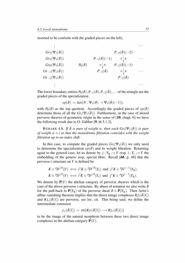
4.3. Local monodromy 77
inserted to be conform with the graded pieces on the left).
... . . .
Gr2(Ψ1(δ )) P−2(δ )(−2)
N∼=
Gr1(Ψ1(δ )) P−1(δ )(−1)
N∼=
. . .
Gr0(Ψ1(δ )) P0(δ ) P−2(δ )(−1)
N∼=
Gr−1(Ψ1(δ )) P−1(δ ) . . .
Gr−2(Ψ1(δ )) P−2(δ )
... . . .
The lower boundary entries P0(δ ),P−1(δ ),P−2(δ ), . . . of the triangle are thegraded pieces of the specialization
sp(δ ) = ker(N : Ψ1(δ )→Ψ1(δ )(−1)),
with P0(δ ) as the top quotient. Accordingly the graded pieces of sp(δ )determine those of all the Gri(Ψ1(δ )). Furthermore, in the case of mixedperverse sheaves of geometric origin in the sense of [10, chapt. 6] we havethe following result due to O. Gabber [9, th 5.1.2].
REMARK 4.8. If δ is pure of weight w, then each Gri(Ψ1(δ )) is pureof weight w+ i so that the monodromy filtration coincides with the weightfiltration up to an index shift.
In this case, to compute the graded pieces Gri(Ψ1(δ )) we only needto determine the specialization sp(δ ) and its weight filtration. Returningagain to the general case, let us denote by j : Yη → Y resp. i : Ys → Y theembedding of the generic resp. special fibre. Recall [60, p. 48] that theperverse t-structure on Y is defined by
K ∈ pD≤0(Y ) ⇐⇒ i∗K ∈ pD≤0(Ys) and j∗K ∈ pD≤−1(Yη),
K ∈ pD≥0(Y ) ⇐⇒ i!K ∈ pD≥0(Ys) and j∗K ∈ pD≥−1(Yη).
We denote by P(Y ) the abelian category of perverse sheaves which is thecore of the above perverse t-structure. By abuse of notation we also write δ
for the pull-back to P(Yη) of the perverse sheaf δ ∈ P(Yη). Then Artin’saffine vanishing theorem implies that the direct image complexes R j!(δ [1])and R j∗(δ [1]) are perverse, see loc. cit. This being said, we define theintermediate extension
j!∗(δ [1]) = im(R j!(δ [1])−→ R j∗(δ [1])
)to be the image of the natural morphism between these two direct imagecomplexes in the abelian category P(Y ).
78 Chapter 4 – The Tannaka group of the theta divisor
LEMMA 4.9. With notations as above, the specialization of δ is givenby the formulae
sp(δ ) = pH0(i∗R j∗(δ )) = i∗( j!∗δ [1])[−1].
Proof. We first claim that in the triangulated category D(Ys)=Dbc (Ys,Λ),
the cone of the morphism N is given by
(?) Cone(Ψ1(δ )
N−→Ψ1(δ )(−1))= i∗R j∗(δ [1]).
Indeed, if we forget about weights, the cone of N on Ψ1(δ ) is isomorphic tothe cone of T −1 on Ψ(δ ) because T −1 is an isomorphism on Ψ 6=1(δ ) andon Ψ1(δ ) its kernel and cokernel are isomorphic to those of N. Hence (?)follows by the same argument as in [60, eq. (3.6.2) and thereafter], usingthat by assumption the wild inertia group P acts trivially on Ψ(δ ). Now iffor n ∈ 0,1 we write
spn(δ ) = pHn(i∗R j∗(δ )),
we obtain from (?) an exact sequence of perverse sheaves
0−→ sp0(δ )−→Ψ1(δ )N−→Ψ1(δ )(−1)−→ sp1(δ )−→ 0.
Hence the first equality in the lemma follows. For the second equality notethat we always have i∗ j!∗(δ [1]) = pτ<0i∗R j∗(δ [1]) by the basic propertiesof the intermediate extension functor shown as in [65, sect. III.5.1], andthat again by (?) the sheaf complex i∗R j∗(δ [1]) is concentrated in perversecohomology degrees −1 and 0.
To connect these local algebraic results to the more global setting ofsection 4.4 below, it will be convenient to reset our notation. So let S be asmooth complex algebraic curve and f : Y −→ S a morphism of complexalgebraic varieties which is smooth over the complement of some givenpoint s ∈ S(C). Consider the strict Henselization S = Spec(O sh
S,s )−→ S of Sat the point s, and let η be the generic point of the strictly Henselian localscheme S. Referring to the base change
f : Y = Y ×S S −→ S
of the morphism f under this strict Henselization, we can form as above thenearby cycles and specialization functors
P(Yη)
Ψ))
sp55P(Ys)
4.4. Degenerations of abelian varieties 79
where Yη and Ys denote the generic resp. special fibres of f . Note that Yscan be naturally identified with the fibre f−1(s) ⊂ Y . In the case of theperverse intersection cohomology sheaf the passage between the global andthe local picture is provided by the following observation, where we nowdenote by i : Ys = f−1(s) → Y the global embedding.
COROLLARY 4.10. In the above situation,
sp(δYη) = i∗(δY [−1]).
Proof. Our smoothness assumption on f implies that the generic fibre Yη
is smooth so that the perverse intersection cohomology sheaf δ = δYηis
the constant sheaf up to a degree shift. From this one easily deduces thatthe intermediate extension j!∗(δ [1]) which occurs in lemma 4.9 arises fromthe perverse intersection cohomology sheaf δY on the total space Y via theHenselization morphism Y −→ Y .
4.4. Degenerations of abelian varieties
To find sufficiently large lower bounds on the general Tannaka groupin theorem 4.2 we consider certain families of ppav’s whose theta divisordegenerates. To construct these we fix an integer n ≥ 3 and work over themoduli space Ag,n of ppav’s of dimension g with level n structure. It hasbeen shown in chapter 7.3 of [80] that this moduli space is representable bya smooth quasi-projective variety over Q. Analytically it can be written asthe quotient
Ag,n(C) = Hg/Γg(n)
of the Siegel upper half space by the action of the principal congruencesubgroup Γg(n) = ker(Sp2g(Z)−→ Sp2g(Z/nZ)). Recall that for n≥ 3 thisaction is free, which again explains why in this case the moduli space issmooth. We denote by
p : X = Hg×Cg / Γg(n)nZ2g // Ag,n
the universal abelian scheme and by Θ ⊂X the divisor which is definedon the universal covering Hg×Cg by the zero locus of the Riemann thetafunction ϑ(τ,z). Thus for each point τ ∈ Ag,n(C) the fibre Xτ = p−1(τ)is a complex ppav with Θτ = Θ∩Xτ as a symmetric theta divisor. Moregenerally, for any complex algebraic variety S with a morphism S−→Ag,nwe denote by
XS = X ×Ag,n S and ΘS = Θ×Ag,n S
80 Chapter 4 – The Tannaka group of the theta divisor
the corresponding abelian scheme resp. its relative theta divisor. For theconstruction of families of ppav’s with degenerating theta divisors we willuse the following general observation.
LEMMA 4.11. For every point s ∈ Ag,n(C) there is a smooth complexquasi-projective curve S → Ag,n, passing through the point s in a generaltangent direction, such that
(a) the generic fibre of the family ΘS→ S is smooth,
(b) the singular loci of the total space and of the special fibre of thisfamily satisfy
Sing(ΘS) ⊆ Sing(Θs).
If the theta divisor Θs contains a singular point of precise multiplicity two,then the inclusion in part (b) is strict for a suitable choice of S.
Proof. Since the moduli space Ag,n is smooth and quasi-projective, forany s ∈ Ag,n(C) we can find a smooth quasi-projective curve S → Ag,npassing through the point s in a general tangent direction. We can assumethat our general curve S is not contained in the locus of ppav’s with singulartheta divisor, indeed by [4] this locus is itself a divisor in Ag,n. So aftershrinking S we can assume that for all t ∈ S(C) \ s the theta divisor Θtis smooth. Then property (a) is clearly satisfied, and property (b) easilyfollows from the fact that the total space ΘS is given locally in the smoothvariety XS as the zero locus of a single analytic function.
Explicitly, let ∆ ⊂ S be an analytic coordinate disk with coordinate wcentered at the given point s, and consider a local lift h : ∆→Hg of theembedding ∆ → S → Ag,n. On the universal covering the divisor ΘS isdescribed as the locus
(w,z) ∈ ∆×Cg | F(w,z) = 0⊂ ∆×Cg
where the analytic function F(w,z) = ϑ(h(w),z) vanishes. If a point (w,z)on this locus defines a singular point of the relative theta divisor ΘS, thenthe gradient of F must vanish at this point. For the gradient in the variable zthis implies
0 = (∇zF)(w,z) = (∇zϑ)(τ,z) for τ = h(w).
Hence (τ,z) defines a singular point of the fibre Θt where t ∈ S(C) denotesthe image of the point τ . By our choice of the curve S the only singularfibre Θt is the one over the point t = s, hence claim (b) follows.
This being said, if some point (τ,z) ∈Hg×Cg defines a singular pointof the theta divisor Θs with precise multiplicity two, then by definition the
4.4. Degenerations of abelian varieties 81
Hesse matrix (∂ 2ϑ
∂ zα∂ zβ
(τ,z))
α,β=1,...,g
is non-zero. Then the heat equation
∂ϑ
∂ταβ
(τ,z) = 2πi · (1+δαβ ) ·∂ 2ϑ
∂ zα∂ zβ
(τ,z)
implies for the gradient with respect to the variable τ that (∇τϑ)(τ,z) 6= 0as well. Hence, taking S to be a curve which passes through the point s ina sufficiently general tangent direction u, we obtain with notations as in thepreceding paragraph that
(∂F/∂w)(0,z) = (u ·∇τϑ)(τ,z) 6= 0
where F(w,z) = ϑ(h(w),z) is defined for w in some coordinate disk ∆⊂ Sby a suitable local lift h : ∆→Hg with h(0) = τ . In particular, since thegradient of F does not vanish at the considered point, it follows that (τ,z)defines a smooth point of the total space ΘS of our family. This shows thatthe inclusion in claim (b) is strict.
We will now use the above construction to obtain information about theTannaka groups G(δΘτ
) by varying the base point τ ∈Ag,n(C). In order toapply the algebraic formalism of nearby cycles developed in section 4.3 weconsider perverse sheaves with coefficients in Λ = Ql throughout, but thefinal result may as well be read in the category of analytic perverse sheaveswith coefficients in Λ = C. Anyway all the occuring perverse sheaves willbe of geometric origin in the sense of [10, sect. 6.2.4].
In general it is not clear how to put the perverse sheaves δΘτfor the
various points τ ∈ Ag,n(C) into a global family because there is no goodrelative notion of a perverse intersection cohomology sheaf. However, overthe Zariski-open dense locus U ⊂Ag,n of ppav’s with a smooth theta divisorthis is no issue — the shifted constant sheaf ΛΘ[g−1] restricts to δΘτ
on thefibre Xτ for each geometric point τ in U . This being said, proposition 3.20shows that there are finitely many reductive algebraic groups G1, . . . ,Gmover Λ and a constructible stratification
U =m⊔
i=0
Ui with G(δΘτ) = Gi for all geometric points τ in Ui.
The hypotheses of the proposition are satisfied because for each geometricpoint τ in U the divisor Θτ ⊂ Xτ is irreducible and symmetric. Indeedthese two conditions precisely say that the perverse sheaf δΘτ
is simple andisomorphic to its adjoint dual.
82 Chapter 4 – The Tannaka group of the theta divisor
Let U0 ⊆U be the open dense stratum so that G0 ⊆G(g) is the Tannakagroup of the theta divisor on a generic ppav. By lemma 4.6 the perverseintersection cohomology sheaf of such a theta divisor corresponds on theTannakian side to the restriction V |G0 of the standard representation V ofthe special orthogonal or symplectic group G(g).
PROPOSITION 4.12. With notations as above, the following propertieshold for the Tannaka groups of smooth theta divisors.
(1) For g = g1 + g2 the generic Tannaka group G0 has a subquotientwhich is isogenous to
G(g1)×G(g2),
provided that theorem 4.2 holds for the dimensions g1 and g2.
(2) There exists a connected subgroup H → G0 and an irreduciblerepresentation W of H such that
V |H =
W ⊕1⊕1 if g is even,W ⊕1 if g is odd,
where 1 denotes the one-dimensional trivial representation.
(3) For g ≥ 4 and any stratum Ui of codimension at most one in Uthere exists a homomorphism
f : Sl2g−2(Λ) −→ Gi
such that f ∗(V ) contains the g−1st fundamental representation ofthe special linear group as a direct summand.
Proof. Consider a morphism from a smooth irreducible quasi-projectivecomplex curve S to the moduli space Ag,n such that the generic point of S ismapped into some stratum Ui in the above stratification, and fix a geometricgeneric point η of S. Passing to the strict Henselization of S at s ∈ S(C)we can form the perverse sheaf Ψ(δΘη
) ∈ Perv(Xs,C) of nearby cycles. Bytheorem 3.15 we have an embedding
G(Ψ(δΘη)) → G(δΘη
) = Gi → G(g)
such that Ψ(δΘη) corresponds on the Tannakian side to the restriction of the
standard representation V to the subgroup G(Ψ(δΘη)). We will apply this
remark in the following situations.
For part (1) take S →Ag,n to be an embedding of a smooth curve whichmeets the locus of decomposable ppav’s in a single point s∈ S(C) but whichis otherwise contained in the open dense stratum U0 and has the properties
4.4. Degenerations of abelian varieties 83
in lemma 4.11. We choose the point s such that the corresponding ppav andits theta divisor have the form
Xs = X1×X2 resp. Θs = (Θ1×X2)∪ (X1×Θ2) ,
where for α ∈ 1,2 the Xα are general complex ppav’s of dimension gα
with a symmetric theta divisor Θα . In particular, like for any divisor withtwo components which intersect each other transversally along a smoothsubvariety, we have an exact sequence
0 −→ δΘ1×Θ2 −→ ΛΘs[g−1] −→ δΘ1×X2⊕δX1×Θ2 −→ 0
of perverse sheaves. Restricting this short exact sequence to the open densesubset
V = Xs \Sing(ΘS) ⊂ Xs
we get a monomorphism
δΘ1×Θ2|V → ΛΘs[g−1]|V = sp(δΘη)|V
of perverse sheaves, where the last equality holds by the formula for thespecialization in corollary 4.10. Now by the last statement in lemma 4.11we can assume that the singular locus Sing(ΘS) is a proper closed subsetof Sing(Θs) = Θ1×Θ2, and in this case the open dense subset V will havenon-empty intersection with Θ1×Θ2. Then via intermediate extension itfollows from the above that the semisimplification of sp(δΘη
) contains adirect summand δΘ1×Θ2 . By the properties of the monodromy filtrationin section 4.3 the same then a fortiori holds for the semisimplification ofthe perverse sheaf of nearby cycles Ψ(δΘη
). This being said, our claimfollows from the elementary observation that the Tannaka group G(δΘ1×Θ2)is isogenous to G(δΘ1)×G(δΘ2).
For part (2) let s ∈ Ag,n(C) be a point which corresponds to a generalppav Xs with a vanishing theta null, and let S → Ag,n be a general curvewhich passes through s but is otherwise contained in the open stratum U0and has the properties in lemma 4.11. For the special fibre with a vanishingtheta null we know from [26] with the correction given in [53, rem. 4.5],or alternatively also from theorem 4.2 of loc. cit., that the theta divisor Θshas an isolated ordinary double point e as its only singularity. Hence thePicard-Lefschetz formula [32, exp. XV, th. 3.4] says that
χ(Θs) = χ(Θη) + (−1)g = (−1)g−1 · (g!−1)
because the generic theta divisor Θη is smooth of dimension g− 1 withEuler characteristic (−1)g−1 · g! by the Gauss-Bonnet theorem. Now theperverse intersection cohomology sheaf near an ordinary double point can
84 Chapter 4 – The Tannaka group of the theta divisor
be controlled explicitly, indeed lemma 4.16 below gives an exact sequenceof perverse sheaves
0 −→ κg −→ ΛΘs[g−1] −→ δΘs −→ 0
for the skyscraper sheaf
κg =
δe(−g−2
2 ) if g is even,0 if g is odd.
Hence it follows that
χ(δΘs) = χ(ΛΘs[g−1])−χ(κg) =
g!−2 if g is even,g!−1 if g is odd.
On the other hand, by remark 4.7 we can assume that the nearby cyclesfor our degeneration coincide with the unipotent nearby cycles. Then fromthe formula for the specialization in corollary 4.10 one deduces that thesemisimplification of the nearby cycles must have the form
Ψ(δΘη)ss = δΘs⊕ γ
for some perverse skyscraper sheaf γ supported on the singular point e ofthe special fibre. Looking at the above Euler characteristics, one sees thatthis skyscraper sheaf γ must have rank two if g is even, resp. rank one if gis odd. Now take a Levi splitting
Gs = G(δΘs) → G(Ψ(δΘη)),
and let W be the irreducible representation of Gs which corresponds to thesimple perverse sheaf δΘs . In lemma 4.13 below we will see as a generalfact about irreducible theta divisors that the restriction of W to the connectedcomponent H = G0
s ⊆ Gs remains irreducible, so our claim follows.
For part (3) consider the locus J ⊂Ag,n of Jacobian varieties of smoothprojective curves of genus g. If a stratum Ui ⊆U has codimension at mostone in the open subset U , then the closure U i ⊆ Ag,n has codimension atmost one in Ag,n. In this case it has been observed in [83, cor. (0.7)] thatthe intersection J∩U i is nonempty and hence of codimension at most onein J. We can then find a point t ∈U i(C) which corresponds to the Jacobianvariety of a non-hyperelliptic smooth curve (indeed the hyperelliptic locushas codimension greater than one in J for g ≥ 4). Now consider in theclosure U i a curve which meets the Jacobian locus J in the chosen point tand is otherwise contained in the open dense subset Ui ⊂U i. Define
ϕ : S −→ Ag,n
to be the normalization of this curve, and choose s ∈ S(C) to be any pointwith ϕ(s) = t. Then XS→ S is a family of ppav’s whose geometric genericfibre Xη is a ppav in the stratum Ui and whose special fibre Xs is the Jacobian
4.5. Proof of the main theorem 85
of a smooth non-hyperelliptic curve. As in lemma 4.11 the singular loci ofthe relative theta divisor ΘS and of the fibre Θs satisfy
Sing(ΘS) ⊆ Sing(Θs),
so it follows from corollary 4.10 that the specialization sp(δΘη) admits the
simple perverse sheaf δΘs as a subquotient. Then the same holds for thenearby cycles Ψ(δΘη
) as well, and this proves our claim since by the resultfor Jacobian varieties in [106], the Brill-Noether sheaf δΘs corresponds tothe g− 1st fundamental representation of its Tannaka group which in thenon-hyperelliptic case is G(δΘs) = Sl2g−2(Λ)/µg−1.
4.5. Proof of the main theorem
Let X be a complex ppav of dimension g and Θ⊂ X a symmetric thetadivisor defining the polarization. Consider the Tannaka group G = G(δΘ)and its representation
V = ω(δΘ) ∈ RepC(G)
which corresponds to the perverse intersection cohomology sheaf δΘ un-der the equivalence ω : 〈δΘ〉 −→ RepC(G) in corollary 3.10. The Tannakagroup does not have to be connected, but fortunately it is not very far frombeing connected either. Indeed we have the following
LEMMA 4.13. If the theta divisor is irreducible, then V restricts to anirreducible representation V |G0 of the connected component G0 ⊆ G.
Proof. The irreducibility of the theta divisor implies that δΘ is a simpleperverse sheaf, and accordingly V is an irreducible representation of theTannaka group G. But by the fundamental result of [109] the group G/G0
is abelian, hence if the claim of our lemma were not true, then by lemma B.4in the appendix we would have an isomorphism V ⊗ χ ∼= V for a suitablenon-trivial character χ : G −→ C∗. The classification of perverse sheaveswith Euler characteristic one in proposition 1.6 shows that χ correspondsto a skyscraper sheaf δx of rank one, supported in some closed point x 6= 0of the ppav X . Hence the above isomorphism would on the geometric sidecorrespond to an isomorphism
δΘ ∗δx ∼= δΘ,
meaning that tx(Θ) = Θ for the translation tx : X → X ,y 7→ y+x. But this isimpossible for any point x 6= 0, indeed the morphism
X −→ Pic0(X), x 7→[OX(Θ− tx(Θ))
]is an isomorphism since the theta divisor gives a principal polarization.
86 Chapter 4 – The Tannaka group of the theta divisor
Now suppose that X is a general ppav. By lemma 4.6 the correspondingTannaka group admits an embedding
G = G(δΘ) → G(g) =
Spg!(C) for even g,SOg!(C) for odd g,
and the representation V = ω(δΘ) arises as the restriction of the standardrepresentation of the classical group on the right hand side. For the proofof theorem 4.2 we will show that for a general ppav the group G must beas large as possible, using the lower bounds in proposition 4.12. We beginwith the following observation.
LEMMA 4.14. For a general ppav X with Tannaka group G = G(δΘ),the connected component G0 ⊆ G is simple modulo its center.
Proof. Let us first introduce some notations. For any reductive complexalgebraic group H consider the derived group H0
der = [H0,H0]. This is aconnected semisimple group, and we denote by
H H0der
its simply connected cover. The covering group H is a product of simplyconnected covers of simple algebraic groups. Furthermore, since by thetheory of reductive groups [100, cor. 8.1.6] the connected component H0 isthe product of its derived group and its center (with finite intersection), anyirreducible representation of H0 is also irreducible under H.
We now return to the Tannaka group G = G(δΘ) for a general ppav. Toprove the lemma we argue by contradiction. If the claim of the lemma is nottrue, then the simply connected cover of this Tannaka group can be writtenin the form
G = G1×G2
for certain non-trivial simply connected groups G1 and G2. Furthermore,for the representation V = ω(δΘ) we have seen in lemma 4.13 that V |G0 isirreducible. Hence by the above remarks also G = G1×G2 acts irreduciblyon V so that we can write
V |G = V1⊗V2
with certain irreducible representations Vi ∈ RepC(Gi). Note that since V isa faithful representation of G, it follows from the definition of the simplyconnected covering group that the representations Vi are non-trivial and inparticular that dim(Vi)> 1. Now consider a connected subgroup H →G asin part (2) of proposition 4.12 so that
V |H = W ⊕
1⊕1 if g is even,1 if g is odd,
4.5. Proof of the main theorem 87
where W is some irreducible representation of the group H. Then via thecommutative diagram
H∃ //
G //
Gl(V1)×Gl(V2)
H // G // Gl(V ) Gl(V1⊗V2)
we can consider the restrictions of V1 and V2 to the covering group H, andby construction we have
V1|H⊗V2|H = V |H = W |H⊕
1⊕1 if g is even,1 if g is odd,
where W |H is irreducible by the general remarks from the beginning of theproof. This implies that both Vi|H are irreducible because otherwise morethan one non-trivial direct summand would occur. But then, since
HomH(1,V1|H⊗V2|H) 6= 0,
adjunction shows V1|H is isomorphic to the dual of V2|H . In particular V1and V2 have the same dimension. This is impossible since dim(V ) = g! isnot the square of a natural number for g > 1.
For g = 4 we can alternatively argue as follows, using only part (3) ofproposition 4.12. Here both V1 and V2 have dimension at most 12 sincetheir dimensions must be non-trivial divisors of dim(V ) = 24. So if insteadof our previous choice we now take the subgroup H → G to be isogenousto Sl2g−2(C) = Sl6(C) with the property in part (3) of the proposition, thenby the classification of small representations in [3] each Vi|H can containonly trivial representations and 6-dimensional standard representations asirreducible constituents. In particular, looking at V1|H ⊗V2|H one sees thatthe third fundamental representation of Sl6(C) cannot occur as a constituentof V |H , and this contradicts our choice of the subgroup H.
Now recall that the Tannaka group G = G(δΘ) of a general ppav is inany case a subgroup of the symplectic or special orthogonal group G(g),hence to prove theorem 4.2 it will be enough to show that the connectedcomponent G0 must be the full group G(g). Note that by lemma 4.13 thisconnected component is an irreducible subgroup of G(g) in the sense thatfor the standard representation V ∈ RepC(G(g)), the restriction V |G0 is stillirreducible. So we are in the situation of the following general lemma.
88 Chapter 4 – The Tannaka group of the theta divisor
LEMMA 4.15. Let H be an irreducible connected subgroup of G(g)which is simple modulo its center. Then
dim(H) ≤ g! or H = G(g).
Proof. Let V denote the standard representation of the symplectic orspecial orthogonal group G(g), and suppose dim(H)> g! = dim(V ). Thenby irreducibility the restriction of V to H must be one of the representationsin table 1 of [3]. Since dim(V ) is the factorial of a natural number, one ofthe following cases must occur for some r ∈ N.
(a) The group H is of type Ar, Cr or Dr and acts on V via its standardrepresentation.
(b) The group H is of type Ar and acts on V via the symmetric or viathe alternating square of its standard representation.
Case (a) can only occur for H = G(g) since G(g) is itself the symplecticor special orthogonal group with V as its standard representation. To dealwith case (b), note that by the criterion in [46, th. 3.2.14] the symmetricsquare of the standard representation of Ar is self-dual only if r = 1, butthen it has dimension 3 6= dim(V ). In the same vein, the alternating squareof the standard representation of Ar is self-dual of dimension g! only in thecase (r,g) = (3,3) where H = G(g) = SO6(C) for dimension reasons.
To complete the proof of theorem 4.2, all that remains to be done is toshow that on a general ppav X we have
dim(G) > g!
for the group G = G(δΘ) attached to the theta divisor. But this follows byinduction on the dimension g = dim(X). Indeed, we already know that thetheorem holds for g ≤ 3, so we can assume g ≥ 4. To start the induction,for g = 4 we can use the subgroup in part (3) of proposition 4.12 since inthat case dim(Sl2g−2(C)) = 35 > g! = 24. This being settled, the inductionstep from dimension g− 1 to dimension g is provided by part (1) of theproposition because dim(G(g−1))> g! for g≥ 5. This finishes the proof ofthe theorem. Going through the above arguments, one furthermore checksthat for g = 4 all we need is part (3) of proposition 4.12. Hence theorem 4.3follows with the same proof.
4.6. Singularities of type Ak
For completeness we include in this section some remarks about doublepoints that have been used in the proof of part (2) of proposition 4.12. In thatproof we have only dealt with ordinary double points, but since this is hardlymore work, in what follows we place ourselves in a slightly more generalsetting. Let Y ⊂ Cn+1 be a complex analytic hypersurface. For k ≥ 1, we
4.6. Singularities of type Ak 89
say that a point e in Y is a singularity of type Ak if in a neighborhood of ethe hypersurface Y is defined by an equation of the form
(?) zk+10 + z2
1 + z22 + · · · + z2
n = 0
in suitable local analytic coordinates (z0, . . . ,zn) on Cn+1 centered at e. Soa singularity of type Ak is just an ordinary double point for k = 1 whereasfor k > 1 it is a double point of corank one.
Working as usual with coefficients in Λ = C or Λ =Ql in the algebraiccase, we want to describe the perverse intersection cohomology sheaf neara singularity of type Ak.
LEMMA 4.16. Let Y ⊂ An+1(C) be a complex analytic hypersurfacewhose only singular point e is a singularity of type Ak.
(a) If k or n is even, then δY = ΛY [n].(b) Otherwise we have an exact sequence of perverse sheaves
0−→ δe(−n−12 )−→ ΛY [n]−→ δY −→ 0.
Proof. We can assume Y is defined by an equation (?). To computethe blowup p : Y −→ Y in the singular point e we choose z = (z0, . . . ,zn)as coordinates on the affine space An+1 = An+1(C). The correspondingcoordinates on Pn = Pn(C) will be denoted u = [u0 : · · · : un]. Then theblowup
Y ⊂ An+1 =(z,u) ∈ An+1×Pn | z ∈ u
can be computed explicitly in the affine charts Ui = (z,u) ∈ An+1 | ui 6= 0with the standard coordinates (u0, . . . ,ui−1,zi,ui+1, . . . ,un) by putting ui = 1and zj = zi uj for j 6= i. Thus
Y ∩U0 =
zk−10 +u2
1 + · · ·+u2n = 0
whereas for i > 0 one obtains that
Y ∩Ui =
uk+10 zk−1
i +u21 + · · ·+u2
i−1 +1+u2i+1 + · · ·+u2
n = 0.
In particular, for k = 1 it follows that the blowup Y is smooth. For k > 1 ithas an isolated singularity e ∈ Y ∩U0 of type Ak−2, and we get by inductionon k an exact sequence
0→ κnk→ ΛY [n]→ δY → 0 where κnk =
0 if 2 | nk,δe(−n−1
2 ) if 2 - nk.
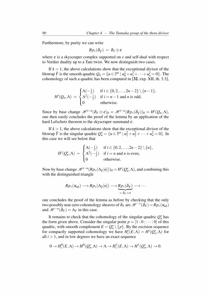
90 Chapter 4 – The Tannaka group of the theta divisor
Furthermore, by purity we can write
Rp∗(δY ) = δY ⊕ ε
where ε is a skyscraper complex supported on e and self-dual with respectto Verdier duality up to a Tate twist. We now distinguish two cases.
If k = 1, the above calculations show that the exceptional divisor of theblowup Y is the smooth quadric Qn = u∈ Pn | u2
0+u21+ · · ·+u2
n = 0. Thecohomology of such a quadric has been computed in [32, exp. XII, th. 3.3],
H i(Qn,Λ) =
Λ(− i
2) if i ∈ 0,2, . . . ,2n−2\n−1,Λ2(− i
2) if i = n−1 and n is odd,0 otherwise.
Since by base change H i−n(δY ⊕ ε)0 = H i−n(Rp∗(δY ))0 = H i(Qn,Λ),one then easily concludes the proof of the lemma by an application of thehard Lefschetz theorem to the skyscraper summand ε .
If k > 1, the above calculations show that the exceptional divisor of theblowup Y is the singular quadric Q?
n = u ∈ Pn | u21 +u2
2 + · · ·+u2n = 0. In
this case we will see below that
H i(Q?n,Λ) =
Λ(− i
2) if i ∈ 0,2, . . . ,2n−2\n,Λ2(− i
2) if i = n and n is even,0 otherwise.
Now by base change H i−n(Rp∗(ΛY [n]))0 = H i(Q?n,Λ), and combining this
with the distinguished triangle
Rp∗(κnk)−→ Rp∗(ΛY [n])−→ Rp∗(δY )︸ ︷︷ ︸= δY ⊕ε
−→ ·· ·
one concludes the proof of the lemma as before by checking that the onlytwo possibly non-zero cohomology sheaves of δY are H −1(δY )=Rp∗(κnk)and H −n(δY ) = ΛY in this case.
It remains to check that the cohomology of the singular quadric Q?n has
the form given above. Consider the singular point p = [1 : 0 : · · · : 0] of thisquadric, with smooth complement E = Q?
n \p. By the excision sequencefor compactly supported cohomology we have H i
c(E,Λ) = H i(Q?n,Λ) for
all i > 1, and in low degrees we have an exact sequence
0→ H0c (E,Λ)→ H0(Q?
n,Λ)→ Λ→ H1c (E,Λ)→ H1(Q?
n,Λ)→ 0.
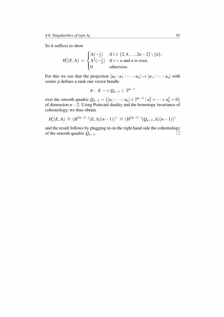
4.6. Singularities of type Ak 91
So it suffices to show
H ic(E,Λ) =
Λ(− i
2) if i ∈ 2,4, . . . ,2n−2\n,Λ2(− i
2) if i = n and n is even,0 otherwise.
For this we use that the projection [u0 : u1 : · · · : un] 7→ [u1 : · · · : un] withcenter p defines a rank one vector bundle
π : E −→ Qn−1 ⊂ Pn−1
over the smooth quadric Qn−1 = [u1 : · · · : un] ∈ Pn−1 | u21 + · · ·+u2
n = 0of dimension n−2. Using Poincare duality and the homotopy invariance ofcohomology, we thus obtain
H ic(E,Λ) ∼= (H2n−2−i(E,Λ)(n−1))∨ ∼= (H2n−2−i(Qn−1,Λ)(n−1))∨
and the result follows by plugging in on the right hand side the cohomologyof the smooth quadric Qn−1.

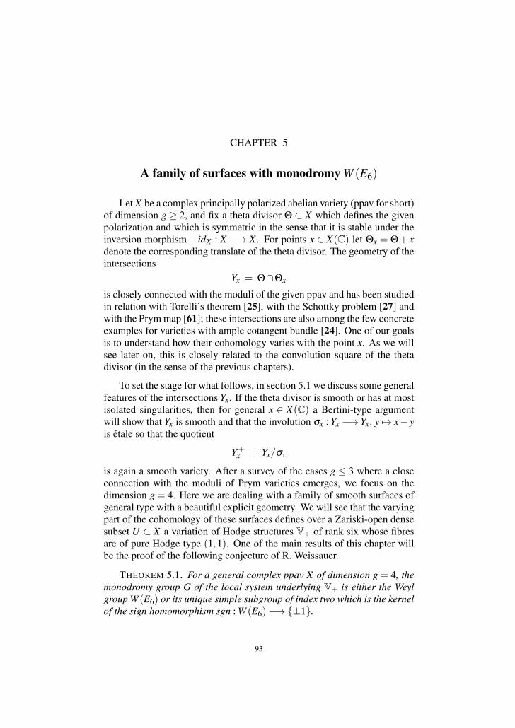
CHAPTER 5
A family of surfaces with monodromy W (E6)
Let X be a complex principally polarized abelian variety (ppav for short)of dimension g ≥ 2, and fix a theta divisor Θ ⊂ X which defines the givenpolarization and which is symmetric in the sense that it is stable under theinversion morphism −idX : X −→ X . For points x ∈ X(C) let Θx = Θ+ xdenote the corresponding translate of the theta divisor. The geometry of theintersections
Yx = Θ∩Θx
is closely connected with the moduli of the given ppav and has been studiedin relation with Torelli’s theorem [25], with the Schottky problem [27] andwith the Prym map [61]; these intersections are also among the few concreteexamples for varieties with ample cotangent bundle [24]. One of our goalsis to understand how their cohomology varies with the point x. As we willsee later on, this is closely related to the convolution square of the thetadivisor (in the sense of the previous chapters).
To set the stage for what follows, in section 5.1 we discuss some generalfeatures of the intersections Yx. If the theta divisor is smooth or has at mostisolated singularities, then for general x ∈ X(C) a Bertini-type argumentwill show that Yx is smooth and that the involution σx : Yx −→ Yx, y 7→ x− yis etale so that the quotient
Y+x = Yx/σx
is again a smooth variety. After a survey of the cases g ≤ 3 where a closeconnection with the moduli of Prym varieties emerges, we focus on thedimension g = 4. Here we are dealing with a family of smooth surfaces ofgeneral type with a beautiful explicit geometry. We will see that the varyingpart of the cohomology of these surfaces defines over a Zariski-open densesubset U ⊂ X a variation of Hodge structures V+ of rank six whose fibresare of pure Hodge type (1,1). One of the main results of this chapter willbe the proof of the following conjecture of R. Weissauer.
THEOREM 5.1. For a general complex ppav X of dimension g = 4, themonodromy group G of the local system underlying V+ is either the Weylgroup W (E6) or its unique simple subgroup of index two which is the kernelof the sign homomorphism sgn : W (E6)−→ ±1.
93
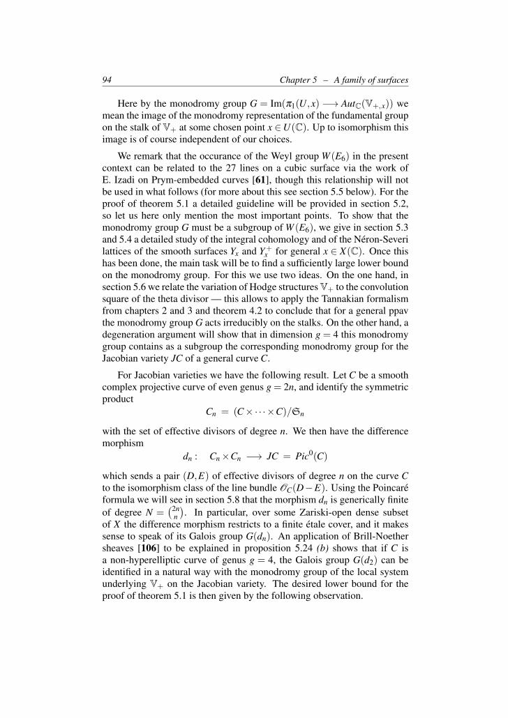
94 Chapter 5 – A family of surfaces
Here by the monodromy group G = Im(π1(U,x) −→ AutC(V+,x)) wemean the image of the monodromy representation of the fundamental groupon the stalk of V+ at some chosen point x ∈U(C). Up to isomorphism thisimage is of course independent of our choices.
We remark that the occurance of the Weyl group W (E6) in the presentcontext can be related to the 27 lines on a cubic surface via the work ofE. Izadi on Prym-embedded curves [61], though this relationship will notbe used in what follows (for more about this see section 5.5 below). For theproof of theorem 5.1 a detailed guideline will be provided in section 5.2,so let us here only mention the most important points. To show that themonodromy group G must be a subgroup of W (E6), we give in section 5.3and 5.4 a detailed study of the integral cohomology and of the Neron-Severilattices of the smooth surfaces Yx and Y+
x for general x ∈ X(C). Once thishas been done, the main task will be to find a sufficiently large lower boundon the monodromy group. For this we use two ideas. On the one hand, insection 5.6 we relate the variation of Hodge structures V+ to the convolutionsquare of the theta divisor — this allows to apply the Tannakian formalismfrom chapters 2 and 3 and theorem 4.2 to conclude that for a general ppavthe monodromy group G acts irreducibly on the stalks. On the other hand, adegeneration argument will show that in dimension g = 4 this monodromygroup contains as a subgroup the corresponding monodromy group for theJacobian variety JC of a general curve C.
For Jacobian varieties we have the following result. Let C be a smoothcomplex projective curve of even genus g = 2n, and identify the symmetricproduct
Cn = (C×·· ·×C)/Sn
with the set of effective divisors of degree n. We then have the differencemorphism
dn : Cn×Cn −→ JC = Pic0(C)
which sends a pair (D,E) of effective divisors of degree n on the curve Cto the isomorphism class of the line bundle OC(D−E). Using the Poincareformula we will see in section 5.8 that the morphism dn is generically finiteof degree N =
(2nn
). In particular, over some Zariski-open dense subset
of X the difference morphism restricts to a finite etale cover, and it makessense to speak of its Galois group G(dn). An application of Brill-Noethersheaves [106] to be explained in proposition 5.24 (b) shows that if C isa non-hyperelliptic curve of genus g = 4, the Galois group G(d2) can beidentified in a natural way with the monodromy group of the local systemunderlying V+ on the Jacobian variety. The desired lower bound for theproof of theorem 5.1 is then given by the following observation.
5.1. Intersections of theta divisors 95
THEOREM 5.2. If C is a general curve of genus g = 2n, then G(dn) iseither the alternating group AN or the full symmetric group SN .
The proof of this in section 5.8 again uses a degeneration, this timefrom a general curve into a hyperelliptic one. We also remark that if theGalois group G(dn) in the above theorem is the full symmetric group SN ,then also the monodromy group G in the previous theorem has to be thefull Weyl group W (E6) because it then contains a reflection. However, atpresent we do not know how to decide whether this is indeed the case.
5.1. Intersections of theta divisors
Consider a complex ppav X of dimension g≥ 2 with a symmetric thetadivisor Θ ⊂ X as above. In this section we will always assume that Θ issmooth or has at most isolated singularities, a situation in which we havethe following Bertini-type result.
LEMMA 5.3. If the theta divisor Θ is smooth or has at most isolatedsingularities, then over some Zariski-open dense subset U ⊂ X there existsa smooth proper family
fU : YU −→ U
whose fibre over any point x ∈U(C) is isomorphic to Yx = Θ∩Θx.
Proof. Recall the general fact [55, cor. III.10.7] that if f : V −→W is amorphism of complex algebraic varieties and if V is smooth, then over someZariski-open dense U ⊆W the restriction fU = f | f−1(U) : f−1(U)−→U isa smooth morphism. Since we can replace W by any Zariski-open densesubset, this remains true if the smoothness assumption on V is replacedby the weaker assumption that the singular locus Sing(V ) is mapped via finto a proper closed subset of W . In the case at hand, we apply this to thecomposite morphism
f : V = Θ×Θ // X×X a // X = W
where a : X ×X −→ X denotes the group law. If the theta divisor has atmost isolated singularities, then Sing(V ) = (Sing(Θ)×Θ)∪ (Θ×Sing(Θ))has dimension g−1 or is empty. In both cases the general fact from aboveshows that over some Zariski-open dense subset U ⊂ X the restriction fUis smooth of relative dimension g− 2. This being said, our claim followsfrom the observation that the projection onto the first factor Θ×Θ −→ Θ
induces an isomorphism f−1(x)∼= Θ∩Θx for x ∈ X(C).
We want to study the fibres Yx of the above family. In this context animportant role is played by the involution σx : X −→ X ,y 7→ x− y. Noticethat the intersection Yx = Θ∩Θx is mapped onto itself by this involution
96 Chapter 5 – A family of surfaces
because we assumed the theta divisor to be symmetric. The above Bertiniargument yields the following
COROLLARY 5.4. If the theta divisor is smooth or has only isolatedsingularities, then there exists a Zariski-open dense subset U ⊂ X such thatfor all x ∈U(C) the quotient morphism
Yx −→ Y+x = Yx/σx
is an etale double covering between smooth varieties of dimension g−2.
Proof. From lemma 5.3 we get a Zariski-open dense subset U ⊂ X suchthat Yx is smooth of dimension g−2 for all x ∈U(C). Shrinking this opendense subset we can furthermore assume that it does not contain points ofthe form x = 2y with y ∈ Θ(C). Then the involution σx : Yx −→ Yx is etalefor all points x ∈U(C), and our claim follows.
For the rest of this section we always fix a point x with the properties inthe above corollary, and we put
Y = Yx, Y+ = Y+x and σ = σx
for brevity. Like for any etale double cover of smooth complex varieties,the rational cohomology of the quotient Y+ coincides with the eigenspacefor the eigenvalue +1 in
H•(Y,Q) = H•(Y,Q)+⊕H•(Y,Q)−
where the upper index ± indicates that the involution σ acts by ±1 on therespective two eigenspaces. Now recall the following version of the weakLefschetz theorem [71, rem. 3.1.29]: If W is a smooth complex projectivevariety of dimension d, then for all ample effective divisors D1, . . . ,Dr therestriction map Hn(W,Z) −→ Hn(D1 ∩ ·· · ∩Dr,Z) is an isomorphism indegrees n < d − r and a monomorphism in degree n = d − r. Note thatthe intersecting divisors are not required to be smooth or transverse to eachother. In our case, since Y is the intersection of two ample divisors on X itfollows that the restriction morphism
Hn(X ,Q) −→ Hn(Y,Q)
is an isomorphism for n < g− 2 and a monomorphism for n = g− 2. Sothe interesting part of the cohomology of Y sits in the middle cohomologydegree n = g−2 and can be defined as the orthocomplement
V = Hg−2(X ,Q)⊥ ⊆ Hg−2(Y,Q)
with respect to the intersection form. The involution σ acts by ε = (−1)g
on Hg−2(X ,Q), hence
Hg−2(X ,Q) ⊆ Hg−2(Y,Q)ε =
Hg−2(Y,Q)+ for g even,Hg−2(Y,Q)− for g odd.
5.1. Intersections of theta divisors 97
So the orthocomplement from above admits a decomposition V =V+⊕V−into the eigenspaces
V−ε = Hg−2(Y,Q)−ε and Vε = Hg−2(X ,Q)⊥ ⊆ Hg−2(Y,Q)ε
where now ⊥ denotes the orthocomplement inside the ε-eigenspace. Sincethe restriction morphism in the weak Lefschetz theorem is a morphism ofHodge structures, V− and V+ are Hodge substructures of Hg−2(Y,Q). Tocompute their Hodge numbers one can use the Hirzebruch-Riemann-Rochtheorem together with the following result, where [Θ] ∈ H2(X ,Q) denotesthe fundamental class of the theta divisor.
LEMMA 5.5. In terms of the restriction θ = [Θ]|Y ∈H2(Y,Q), the Chernclasses of Y are given by
ci(Y ) = (−1)i · (i+1) ·θ i ∈ H2i(Y,Q).
In particular, the variety Y is of general type with canonical class KY = 2θ .
Proof. By definition we have Y = Θ∩Θx for some point x ∈ X(C). Theembedding Y →Θ gives an adjunction sequence
0−→TY −→TΘ|Y −→ OX(Θx)|Y −→ 0
where TY and TΘ are the tangent bundles to Y resp. Θ (note that this makessense also if the theta divisor has isolated singularities, provided that x ischosen in such a way that Y does not meet the singularities). By restrictionof the adjunction sequence for the embedding Θ → X we also get an exactsequence
0−→TΘ|Y −→TX |Y −→ OX(Θ)|Y −→ 0.Since the tangent bundle TX is trivial, it follows from these two adjunctionsequences that the Chern polynomial ct(Y ) = 1+ c1(Y ) · t + c2(Y ) · t2 + · · ·satisfies
1 = ct(Y ) · (1+θ t)2
since the Chern polynomial is multiplicative in short exact sequences. Fromthis identity our claim about the Chern classes follows by a comparison ofcoefficients. By definition the canonical sheaf ωY is the top exterior powerof the cotangent bundle T ∗
Y , so for the canonical class we get
KY = c1(ωY ) = c1(Λg−2(T ∗
Y )) = c1(T∗
Y ) = −c1(Y ) = 2θ
where in the third equality we have used that by the splitting principle thefirst Chern class of a bundle coincides with the first Chern class of any ofits exterior powers [40, rem. 3.2.3(c)]. In particular, the canonical class KYis ample and therefore also big in the sense of [71, sect. 2.2], so the smoothvariety Y is of general type.
With notations as in the above lemma, to compute intersection numbersbetween powers of Chern classes we only need to determine the image of
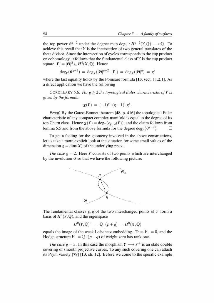
98 Chapter 5 – A family of surfaces
the top power θ g−2 under the degree map degY : Hg−2(Y,Q) −→ Q. Toachieve this recall that Y is the intersection of two general translates of thetheta divisor. Since the intersection of cycles corresponds to the cup producton cohomology, it follows that the fundamental class of Y is the cup productsquare [Y ] = [Θ]2 ∈ H4(X ,Q). Hence
degY (θg−2) = degX([Θ]g−2 · [Y ]) = degX([Θ]g) = g!
where the last equality holds by the Poincare formula [13, sect. 11.2.1]. Asa direct application we have the following
COROLLARY 5.6. For g≥ 2 the topological Euler characteristic of Y isgiven by the formula
χ(Y ) = (−1)g · (g−1) ·g! .
Proof. By the Gauss-Bonnet theorem [48, p. 416] the topological Eulercharacteristic of any compact complex manifold is equal to the degree of itstop Chern class. Hence χ(Y ) = degY (cg−2(Y )), and the claim follows fromlemma 5.5 and from the above formula for the degree degY (θ
g−2).
To get a feeling for the geometry involved in the above constructions,let us take a more explicit look at the situation for some small values of thedimension g = dim(X) of the underlying ppav.
The case g = 2. Here Y consists of two points which are interchangedby the involution σ so that we have the following picture.
ss
p
q
AAU
K
Θ
Θx
The fundamental classes p,q of the two interchanged points of Y form abasis of H0(Y,Q), and the eigenspace
H0(Y,Q)+ = Q · (p+q) = H0(X ,Q)
equals the image of the weak Lefschetz embedding. Thus V+ = 0, and theHodge structure V− =Q · (p−q) of weight zero has rank one.
The case g = 3. In this case the morphism Y −→ Y+ is an etale doublecovering of smooth projective curves. To any such covering one can attachits Prym variety [79] [13, ch. 12]. Before we come to the specific example
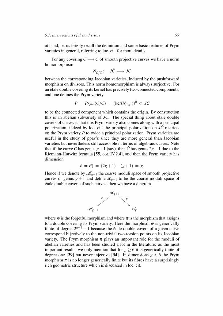
5.1. Intersections of theta divisors 99
at hand, let us briefly recall the definition and some basic features of Prymvarieties in general, referring to loc. cit. for more details.
For any covering C −→C of smooth projective curves we have a normhomomorphism
NC/C : JC −→ JC
between the corresponding Jacobian varieties, induced by the pushforwardmorphism on divisors. This norm homomorphism is always surjective. Foran etale double covering its kernel has precisely two connected components,and one defines the Prym variety
P = Prym(C/C) = (ker(NC/C))0 ⊂ JC
to be the connected component which contains the origin. By constructionthis is an abelian subvariety of JC. The special thing about etale doublecovers of curves is that this Prym variety also comes along with a principalpolarization, indeed by loc. cit. the principal polarization on JC restrictson the Prym variety P to twice a principal polarization. Prym varieties areuseful in the study of ppav’s since they are more general than Jacobianvarieties but nevertheless still accessible in terms of algebraic curves. Notethat if the curve C has genus g+1 (say), then C has genus 2g+1 due to theRiemann-Hurwitz formula [55, cor. IV.2.4], and then the Prym variety hasdimension
dim(P) = (2g+1)− (g+1) = g.
Hence if we denote by Mg+1 the coarse moduli space of smooth projectivecurves of genus g+ 1 and define Rg+1 to be the coarse moduli space ofetale double covers of such curves, then we have a diagram
Rg+1ϕ
vvvvv
vvvv π
""DDD
DDDD
D
Mg+1 Ag
where ϕ is the forgetful morphism and where π is the morphism that assignsto a double covering its Prym variety. Here the morphism ϕ is genericallyfinite of degree 2g+1− 1 because the etale double covers of a given curvecorrespond bijectively to the non-trivial two-torsion points on its Jacobianvariety. The Prym morphism π plays an important role for the moduli ofabelian varieties and has been studied a lot in the literature; as the mostimportant results, we only mention that for g ≥ 6 it is generically finite ofdegree one [39] but never injective [34]. In dimensions g < 6 the Prymmorphism π is no longer generically finite but its fibres have a surprisinglyrich geometric structure which is discussed in loc. cit.
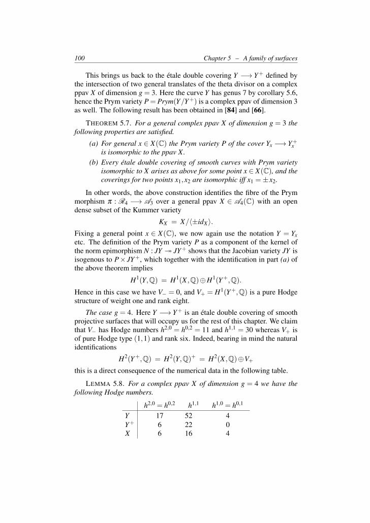
100 Chapter 5 – A family of surfaces
This brings us back to the etale double covering Y −→ Y+ defined bythe intersection of two general translates of the theta divisor on a complexppav X of dimension g = 3. Here the curve Y has genus 7 by corollary 5.6,hence the Prym variety P = Prym(Y/Y+) is a complex ppav of dimension 3as well. The following result has been obtained in [84] and [66].
THEOREM 5.7. For a general complex ppav X of dimension g = 3 thefollowing properties are satisfied.
(a) For general x ∈ X(C) the Prym variety P of the cover Yx −→ Y+x
is isomorphic to the ppav X.(b) Every etale double covering of smooth curves with Prym variety
isomorphic to X arises as above for some point x ∈ X(C), and thecoverings for two points x1,x2 are isomorphic iff x1 =±x2.
In other words, the above construction identifies the fibre of the Prymmorphism π : R4 −→ A3 over a general ppav X ∈ A4(C) with an opendense subset of the Kummer variety
KX = X/〈±idX〉.Fixing a general point x ∈ X(C), we now again use the notation Y = Yxetc. The definition of the Prym variety P as a component of the kernel ofthe norm epimorphism N : JY JY+ shows that the Jacobian variety JY isisogenous to P× JY+, which together with the identification in part (a) ofthe above theorem implies
H1(Y,Q) = H1(X ,Q)⊕H1(Y+,Q).
Hence in this case we have V− = 0, and V+ = H1(Y+,Q) is a pure Hodgestructure of weight one and rank eight.
The case g = 4. Here Y −→ Y+ is an etale double covering of smoothprojective surfaces that will occupy us for the rest of this chapter. We claimthat V− has Hodge numbers h2,0 = h0,2 = 11 and h1,1 = 30 whereas V+ isof pure Hodge type (1,1) and rank six. Indeed, bearing in mind the naturalidentifications
H2(Y+,Q) = H2(Y,Q)+ = H2(X ,Q)⊕V+
this is a direct consequence of the numerical data in the following table.
LEMMA 5.8. For a complex ppav X of dimension g = 4 we have thefollowing Hodge numbers.
h2,0 = h0,2 h1,1 h1,0 = h0,1
Y 17 52 4Y+ 6 22 0X 6 16 4
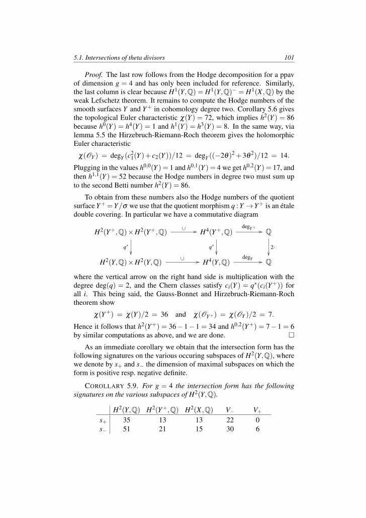
5.1. Intersections of theta divisors 101
Proof. The last row follows from the Hodge decomposition for a ppavof dimension g = 4 and has only been included for reference. Similarly,the last column is clear because H1(Y,Q) = H1(Y,Q)− = H1(X ,Q) by theweak Lefschetz theorem. It remains to compute the Hodge numbers of thesmooth surfaces Y and Y+ in cohomology degree two. Corollary 5.6 givesthe topological Euler characteristic χ(Y ) = 72, which implies h2(Y ) = 86because h0(Y ) = h4(Y ) = 1 and h1(Y ) = h3(Y ) = 8. In the same way, vialemma 5.5 the Hirzebruch-Riemann-Roch theorem gives the holomorphicEuler characteristic
χ(OY ) = degY (c21(Y )+ c2(Y ))/12 = degY ((−2θ)2 +3θ
2)/12 = 14.
Plugging in the values h0,0(Y ) = 1 and h0,1(Y ) = 4 we get h0,2(Y ) = 17, andthen h1,1(Y ) = 52 because the Hodge numbers in degree two must sum upto the second Betti number h2(Y ) = 86.
To obtain from these numbers also the Hodge numbers of the quotientsurface Y+ =Y/σ we use that the quotient morphism q : Y →Y+ is an etaledouble covering. In particular we have a commutative diagram
H2(Y+,Q)×H2(Y+,Q)∪ //
q∗
H4(Y+,Q)degY+ //
q∗
Q
2·
H2(Y,Q)×H2(Y,Q)∪ // H4(Y,Q)
degY // Q
where the vertical arrow on the right hand side is multiplication with thedegree deg(q) = 2, and the Chern classes satisfy ci(Y ) = q∗(ci(Y+)) forall i. This being said, the Gauss-Bonnet and Hirzebruch-Riemann-Rochtheorem show
χ(Y+) = χ(Y )/2 = 36 and χ(OY+) = χ(OY )/2 = 7.
Hence it follows that h2(Y+) = 36− 1− 1 = 34 and h0,2(Y+) = 7− 1 = 6by similar computations as above, and we are done.
As an immediate corollary we obtain that the intersection form has thefollowing signatures on the various occuring subspaces of H2(Y,Q), wherewe denote by s+ and s− the dimension of maximal subspaces on which theform is positive resp. negative definite.
COROLLARY 5.9. For g = 4 the intersection form has the followingsignatures on the various subspaces of H2(Y,Q).
H2(Y,Q) H2(Y+,Q) H2(X ,Q) V− V+
s+ 35 13 13 22 0s− 51 21 15 30 6
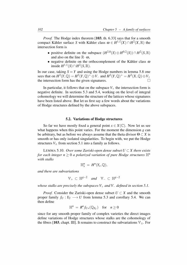
102 Chapter 5 – A family of surfaces
Proof. The Hodge index theorem [103, th. 6.33] says that for a smoothcompact Kahler surface S with Kahler class ω ∈ H1,1(X)∩H2(X ,R) theintersection form is
• positive definite on the subspace (H2,0(S)⊕H0,2(S))∩H2(S,R)and also on the line R ·ω ,• negative definite on the orthocomplement of the Kahler class ω
inside H1,1(S)∩H2(S,R).In our case, taking S = Y and using the Hodge numbers in lemma 5.8 onesees that on H2(Y,Q) = H2(Y,Q)+⊕V− and H2(Y,Q)+ = H2(X ,Q)⊕V+
the intersection form has the given signatures.
In particular, it follows that on the subspace V+ the intersection form isnegative definite. In sections 5.3 and 5.4, working on the level of integralcohomology we will determine the structure of the lattices whose signatureshave been listed above. But let us first say a few words about the variationsof Hodge structures defined by the above subspaces.
5.2. Variations of Hodge structures
So far we have mostly fixed a general point x ∈ X(C). Now let us seewhat happens when this point varies. For the moment the dimension g canbe arbitrary, but as before we always assume that the theta divisor Θ⊂ X issmooth or has only isolated singularities. To begin with, we put the Hodgestructures V± from section 5.1 into a family as follows.
LEMMA 5.10. Over some Zariski-open dense subset U ⊂ X there existsfor each integer n ≥ 0 a polarized variation of pure Hodge structures Hn
with stalks
Hnx = Hn(Yx,Q),
and there are subvariations
V+ ⊂ Hg−2 and V− ⊂ Hg−2
whose stalks are precisely the subspaces V+ and V− defined in section 5.1.
Proof. Consider the Zariski-open dense subset U ⊂ X and the smoothproper family fU : YU −→ U from lemma 5.3 and corollary 5.4. We canthen define
Hn = Rn fU∗(QYU ) for n≥ 0
since for any smooth proper family of complex varieties the direct imagesdefine variations of Hodge structures whose stalks are the cohomology ofthe fibres [103, chapt. III]. It remains to construct the subvariations V±. For
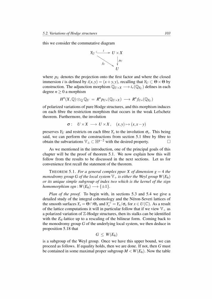
5.2. Variations of Hodge structures 103
this we consider the commutative diagram
YU i //
fU %%JJJJJJJJJJJJ U×X
pU
U
where pU denotes the projection onto the first factor and where the closedimmersion i is defined by i(x,y) = (x+ y,y), recalling that YU ⊂ Θ×Θ byconstruction. The adjunction morphism QU×X −→ i∗(QYU ) defines in eachdegree n≥ 0 a morphism
Hn(X ,Q)⊗QQU = Rn pU∗(QU×X) −→ Rn fU∗(QYU )
of polarized variations of pure Hodge structures, and this morphism induceson each fibre the restriction morphism that occurs in the weak Lefschetztheorem. Furthermore, the involution
σ : U×X −→ U×X , (x,y) 7→ (x,x− y)
preserves YU and restricts on each fibre Yx to the involution σx. This beingsaid, we can perform the constructions from section 5.1 fibre by fibre toobtain the subvariations V± ⊂Hg−2 with the desired property.
As we mentioned in the introduction, one of the principal goals of thischapter will be the proof of theorem 5.1. We now explain how this willfollow from the results to be discussed in the next sections. Let us forconvenience first recall the statement of the theorem.
THEOREM 5.1. For a general complex ppav X of dimension g = 4 themonodromy group G of the local system V+ is either the Weyl group W (E6)or its unique simple subgroup of index two which is the kernel of the signhomomorphism sgn : W (E6)−→ ±1.
Plan of the proof. To begin with, in sections 5.3 and 5.4 we give adetailed study of the integral cohomology and the Neron-Severi lattices ofthe smooth surfaces Yx = Θ∩Θx and Y+
x =Yx/σx for x ∈U(C). As a resultof the lattice computations it will in particular follow that if we view V+ asa polarized variation of Z-Hodge structures, then its stalks can be identifiedwith the E6-lattice up to a rescaling of the bilinear form. Coming back tothe monodromy group G of the underlying local system, we then deduce inproposition 5.18 that
G ≤ W (E6)
is a subgroup of the Weyl group. Once we have this upper bound, we canproceed as follows. If equality holds, then we are done. If not, then G mustbe contained in some maximal proper subgroup M <W (E6). Now the table
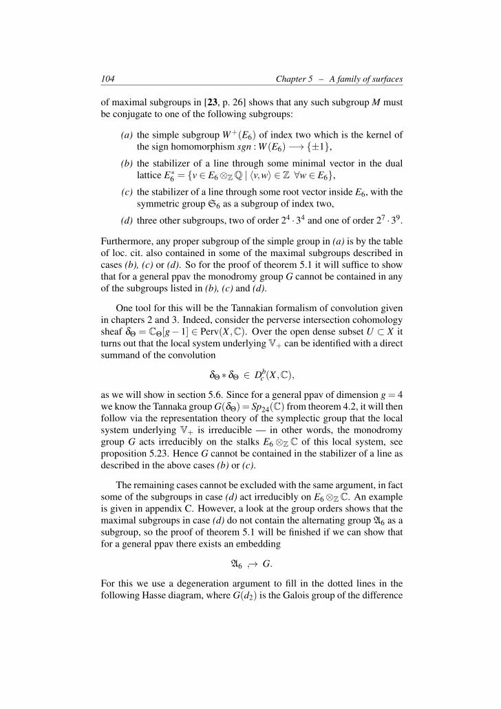
104 Chapter 5 – A family of surfaces
of maximal subgroups in [23, p. 26] shows that any such subgroup M mustbe conjugate to one of the following subgroups:
(a) the simple subgroup W+(E6) of index two which is the kernel ofthe sign homomorphism sgn : W (E6)−→ ±1,
(b) the stabilizer of a line through some minimal vector in the duallattice E∗6 = v ∈ E6⊗ZQ | 〈v,w〉 ∈ Z ∀w ∈ E6,
(c) the stabilizer of a line through some root vector inside E6, with thesymmetric group S6 as a subgroup of index two,
(d) three other subgroups, two of order 24 ·34 and one of order 27 ·39.
Furthermore, any proper subgroup of the simple group in (a) is by the tableof loc. cit. also contained in some of the maximal subgroups described incases (b), (c) or (d). So for the proof of theorem 5.1 it will suffice to showthat for a general ppav the monodromy group G cannot be contained in anyof the subgroups listed in (b), (c) and (d).
One tool for this will be the Tannakian formalism of convolution givenin chapters 2 and 3. Indeed, consider the perverse intersection cohomologysheaf δΘ = CΘ[g− 1] ∈ Perv(X ,C). Over the open dense subset U ⊂ X itturns out that the local system underlying V+ can be identified with a directsummand of the convolution
δΘ ∗δΘ ∈ Dbc (X ,C),
as we will show in section 5.6. Since for a general ppav of dimension g = 4we know the Tannaka group G(δΘ)= Sp24(C) from theorem 4.2, it will thenfollow via the representation theory of the symplectic group that the localsystem underlying V+ is irreducible — in other words, the monodromygroup G acts irreducibly on the stalks E6⊗Z C of this local system, seeproposition 5.23. Hence G cannot be contained in the stabilizer of a line asdescribed in the above cases (b) or (c).
The remaining cases cannot be excluded with the same argument, in factsome of the subgroups in case (d) act irreducibly on E6⊗ZC. An exampleis given in appendix C. However, a look at the group orders shows that themaximal subgroups in case (d) do not contain the alternating group A6 as asubgroup, so the proof of theorem 5.1 will be finished if we can show thatfor a general ppav there exists an embedding
A6 → G.
For this we use a degeneration argument to fill in the dotted lines in thefollowing Hasse diagram, where G(d2) is the Galois group of the difference
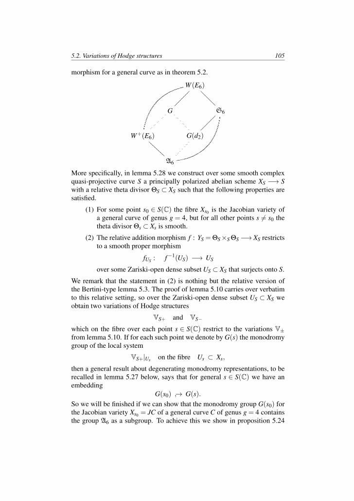
5.2. Variations of Hodge structures 105
morphism for a general curve as in theorem 5.2.
W (E6)
G
S6
???????
W+(E6) G(d2)
A6
AAAAAAAA
More specifically, in lemma 5.28 we construct over some smooth complexquasi-projective curve S a principally polarized abelian scheme XS −→ Swith a relative theta divisor ΘS ⊂ XS such that the following properties aresatisfied.
(1) For some point s0 ∈ S(C) the fibre Xs0 is the Jacobian variety ofa general curve of genus g = 4, but for all other points s 6= s0 thetheta divisor Θs ⊂ Xs is smooth.
(2) The relative addition morphism f : YS = ΘS×S ΘS −→ XS restrictsto a smooth proper morphism
fUS : f−1(US) −→ US
over some Zariski-open dense subset US ⊂ XS that surjects onto S.
We remark that the statement in (2) is nothing but the relative version ofthe Bertini-type lemma 5.3. The proof of lemma 5.10 carries over verbatimto this relative setting, so over the Zariski-open dense subset US ⊂ XS weobtain two variations of Hodge structures
VS+ and VS−
which on the fibre over each point s ∈ S(C) restrict to the variations V±from lemma 5.10. If for each such point we denote by G(s) the monodromygroup of the local system
VS+|Us on the fibre Us ⊂ Xs,
then a general result about degenerating monodromy representations, to berecalled in lemma 5.27 below, says that for general s ∈ S(C) we have anembedding
G(s0) → G(s).So we will be finished if we can show that the monodromy group G(s0) forthe Jacobian variety Xs0 = JC of a general curve C of genus g = 4 containsthe group A6 as a subgroup. To achieve this we show in proposition 5.24
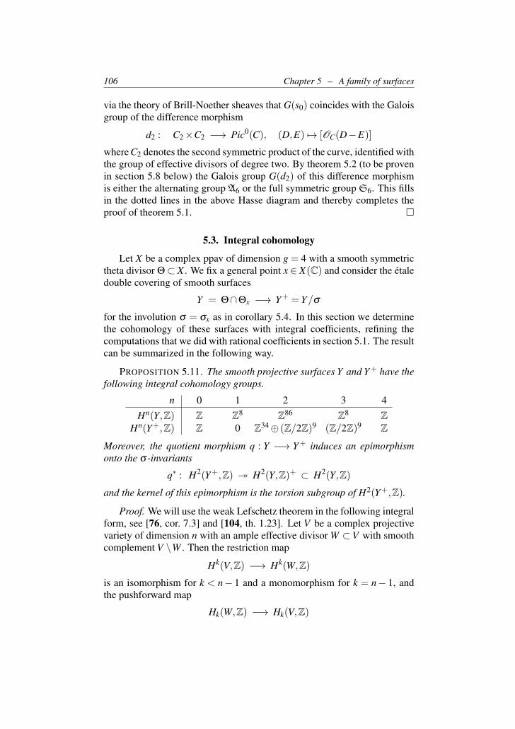
106 Chapter 5 – A family of surfaces
via the theory of Brill-Noether sheaves that G(s0) coincides with the Galoisgroup of the difference morphism
d2 : C2×C2 −→ Pic0(C), (D,E) 7→ [OC(D−E)]
where C2 denotes the second symmetric product of the curve, identified withthe group of effective divisors of degree two. By theorem 5.2 (to be provenin section 5.8 below) the Galois group G(d2) of this difference morphismis either the alternating group A6 or the full symmetric group S6. This fillsin the dotted lines in the above Hasse diagram and thereby completes theproof of theorem 5.1.
5.3. Integral cohomology
Let X be a complex ppav of dimension g = 4 with a smooth symmetrictheta divisor Θ⊂ X . We fix a general point x ∈ X(C) and consider the etaledouble covering of smooth surfaces
Y = Θ∩Θx −→ Y+ = Y/σ
for the involution σ = σx as in corollary 5.4. In this section we determinethe cohomology of these surfaces with integral coefficients, refining thecomputations that we did with rational coefficients in section 5.1. The resultcan be summarized in the following way.
PROPOSITION 5.11. The smooth projective surfaces Y and Y+ have thefollowing integral cohomology groups.
n 0 1 2 3 4Hn(Y,Z) Z Z8 Z86 Z8 Z
Hn(Y+,Z) Z 0 Z34⊕ (Z/2Z)9 (Z/2Z)9 Z
Moreover, the quotient morphism q : Y −→ Y+ induces an epimorphismonto the σ -invariants
q∗ : H2(Y+,Z) H2(Y,Z)+ ⊂ H2(Y,Z)
and the kernel of this epimorphism is the torsion subgroup of H2(Y+,Z).
Proof. We will use the weak Lefschetz theorem in the following integralform, see [76, cor. 7.3] and [104, th. 1.23]. Let V be a complex projectivevariety of dimension n with an ample effective divisor W ⊂V with smoothcomplement V \W . Then the restriction map
Hk(V,Z) −→ Hk(W,Z)is an isomorphism for k < n− 1 and a monomorphism for k = n− 1, andthe pushforward map
Hk(W,Z) −→ Hk(V,Z)
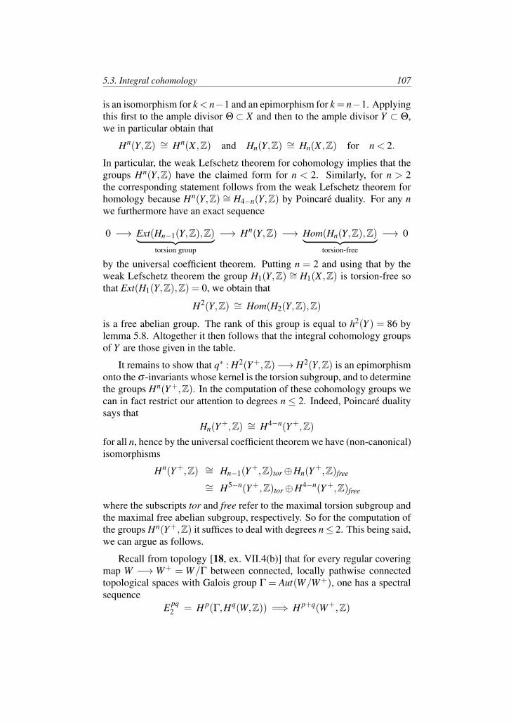
5.3. Integral cohomology 107
is an isomorphism for k < n−1 and an epimorphism for k = n−1. Applyingthis first to the ample divisor Θ ⊂ X and then to the ample divisor Y ⊂ Θ,we in particular obtain that
Hn(Y,Z) ∼= Hn(X ,Z) and Hn(Y,Z) ∼= Hn(X ,Z) for n < 2.
In particular, the weak Lefschetz theorem for cohomology implies that thegroups Hn(Y,Z) have the claimed form for n < 2. Similarly, for n > 2the corresponding statement follows from the weak Lefschetz theorem forhomology because Hn(Y,Z) ∼= H4−n(Y,Z) by Poincare duality. For any nwe furthermore have an exact sequence
0 −→ Ext(Hn−1(Y,Z),Z)︸ ︷︷ ︸torsion group
−→ Hn(Y,Z) −→ Hom(Hn(Y,Z),Z)︸ ︷︷ ︸torsion-free
−→ 0
by the universal coefficient theorem. Putting n = 2 and using that by theweak Lefschetz theorem the group H1(Y,Z) ∼= H1(X ,Z) is torsion-free sothat Ext(H1(Y,Z),Z) = 0, we obtain that
H2(Y,Z) ∼= Hom(H2(Y,Z),Z)
is a free abelian group. The rank of this group is equal to h2(Y ) = 86 bylemma 5.8. Altogether it then follows that the integral cohomology groupsof Y are those given in the table.
It remains to show that q∗ : H2(Y+,Z)−→H2(Y,Z) is an epimorphismonto the σ -invariants whose kernel is the torsion subgroup, and to determinethe groups Hn(Y+,Z). In the computation of these cohomology groups wecan in fact restrict our attention to degrees n ≤ 2. Indeed, Poincare dualitysays that
Hn(Y+,Z) ∼= H4−n(Y+,Z)for all n, hence by the universal coefficient theorem we have (non-canonical)isomorphisms
Hn(Y+,Z) ∼= Hn−1(Y+,Z)tor⊕Hn(Y+,Z)free
∼= H5−n(Y+,Z)tor⊕H4−n(Y+,Z)free
where the subscripts tor and free refer to the maximal torsion subgroup andthe maximal free abelian subgroup, respectively. So for the computation ofthe groups Hn(Y+,Z) it suffices to deal with degrees n≤ 2. This being said,we can argue as follows.
Recall from topology [18, ex. VII.4(b)] that for every regular coveringmap W −→W+ = W/Γ between connected, locally pathwise connectedtopological spaces with Galois group Γ = Aut(W/W+), one has a spectralsequence
E pq2 = H p(Γ,Hq(W,Z)) =⇒ H p+q(W+,Z)
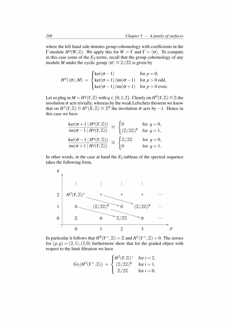
108 Chapter 5 – A family of surfaces
where the left hand side denotes group cohomology with coefficients in theΓ-module Hq(W,Z). We apply this for W = Y and Γ = 〈σ〉. To computein this case some of the E2-terms, recall that the group cohomology of anymodule M under the cyclic group 〈σ〉 ∼= Z/2Z is given by
H p(〈σ〉,M) =
ker(σ −1) for p = 0,ker(σ +1)/im(σ −1) for p > 0 odd,ker(σ −1)/im(σ +1) for p > 0 even.
Let us plug in M =Hq(Y,Z) with q∈ 0,1,2. Clearly on H0(Y,Z)∼=Z theinvolution σ acts trivially, whereas by the weak Lefschetz theorem we knowthat on H1(Y,Z) ∼= H1(X ,Z) ∼= Z8 the involution σ acts by −1. Hence inthis case we have
ker(σ +1 | Hq(Y,Z))im(σ −1 | Hq(Y,Z))
∼=
0 for q = 0,(Z/2Z)8 for q = 1,
ker(σ −1 | Hq(Y,Z))im(σ +1 | Hq(Y,Z))
∼=
Z/2Z for q = 0,0 for q = 1.
In other words, in the case at hand the E2-tableau of the spectral sequencetakes the following form.
q
......
......
2 H2(Y,Z)+
++WWWWWWWWWWWWWWWWWW ∗
**VVVVVVVVVVVVVVVVV ∗ ∗ · · ·
1 0
++WWWWWWWWWWWWWWWWWWWW (Z/2Z)8
++VVVVVVVVVVVVVVVVV 0 (Z/2Z)8 · · ·
0 Z 0 Z/2Z 0 · · ·//
OO
0 1 2 3 p
In particular it follows that H0(Y+,Z) = Z and H1(Y+,Z) = 0. The zeroesfor (p,q) = (2,1),(3,0) furthermore show that for the graded object withrespect to the limit filtration we have
Gri(H2(Y+,Z)) =
H2(Y,Z)+ for i = 2,(Z/2Z)8 for i = 1,Z/2Z for i = 0,
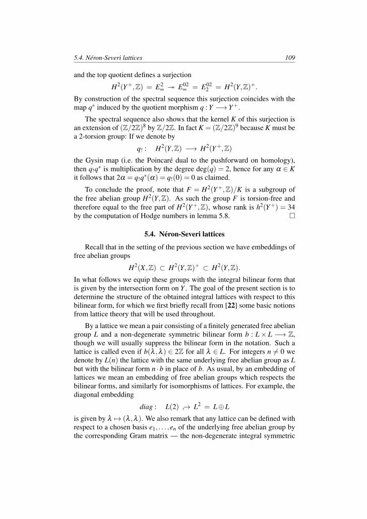
5.4. Neron-Severi lattices 109
and the top quotient defines a surjection
H2(Y+,Z) = E2∞ E02
∞ = E022 = H2(Y,Z)+.
By construction of the spectral sequence this surjection coincides with themap q∗ induced by the quotient morphism q : Y −→ Y+.
The spectral sequence also shows that the kernel K of this surjection isan extension of (Z/2Z)8 by Z/2Z. In fact K = (Z/2Z)9 because K must bea 2-torsion group: If we denote by
q! : H2(Y,Z) −→ H2(Y+,Z)the Gysin map (i.e. the Poincare dual to the pushforward on homology),then q!q∗ is multiplication by the degree deg(q) = 2, hence for any α ∈ Kit follows that 2α = q!q∗(α) = q!(0) = 0 as claimed.
To conclude the proof, note that F = H2(Y+,Z)/K is a subgroup ofthe free abelian group H2(Y,Z). As such the group F is torsion-free andtherefore equal to the free part of H2(Y+,Z), whose rank is h2(Y+) = 34by the computation of Hodge numbers in lemma 5.8.
5.4. Neron-Severi lattices
Recall that in the setting of the previous section we have embeddings offree abelian groups
H2(X ,Z) ⊂ H2(Y,Z)+ ⊂ H2(Y,Z).In what follows we equip these groups with the integral bilinear form thatis given by the intersection form on Y . The goal of the present section is todetermine the structure of the obtained integral lattices with respect to thisbilinear form, for which we first briefly recall from [22] some basic notionsfrom lattice theory that will be used throughout.
By a lattice we mean a pair consisting of a finitely generated free abeliangroup L and a non-degenerate symmetric bilinear form b : L× L −→ Z,though we will usually suppress the bilinear form in the notation. Such alattice is called even if b(λ ,λ ) ∈ 2Z for all λ ∈ L. For integers n 6= 0 wedenote by L(n) the lattice with the same underlying free abelian group as Lbut with the bilinear form n ·b in place of b. As usual, by an embedding oflattices we mean an embedding of free abelian groups which respects thebilinear forms, and similarly for isomorphisms of lattices. For example, thediagonal embedding
diag : L(2) → L2 = L⊕L
is given by λ 7→ (λ ,λ ). We also remark that any lattice can be defined withrespect to a chosen basis e1, . . . ,en of the underlying free abelian group bythe corresponding Gram matrix — the non-degenerate integral symmetric
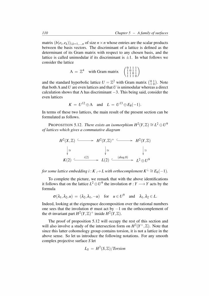
110 Chapter 5 – A family of surfaces
matrix (b(ei,ek))i,k=1,...,n of size n×n whose entries are the scalar productsbetween the basis vectors. The discriminant of a lattice is defined as thedeterminant of its Gram matrix with respect to any chosen basis, and thelattice is called unimodular if its discriminant is ±1. In what follows weconsider the lattice
Λ = Z4 with Gram matrix(0 1 1 1
1 0 1 11 1 0 11 1 1 0
)and the standard hyperbolic lattice U = Z2 with Gram matrix
(0 11 0
). Note
that both Λ and U are even lattices and that U is unimodular whereas a directcalculation shows that Λ has discriminant−3. This being said, consider theeven lattices
K = U12⊕Λ and L = U13⊕E8(−1).
In terms of these two lattices, the main result of the present section can beformulated as follows.
PROPOSITION 5.12. There exists an isomorphism H2(Y,Z) ∼= L2⊕U9
of lattices which gives a commutative diagram
H2(X ,Z) //
∼=
H2(Y,Z)+ //
∼=
H2(Y,Z)
∼=
K(2) i(2)// L(2) (diag,0)
// L2⊕U9
for some lattice embedding i : K → L with orthocomplement K⊥ ∼= E6(−1).
To complete the picture, we remark that with the above identificationsit follows that on the lattice L2⊕U9 the involution σ : Y −→ Y acts by theformula
σ(λ1,λ2,u) = (λ2,λ1,−u) for u ∈U9 and λ1,λ2 ∈ L.
Indeed, looking at the eigenspace decomposition over the rational numbersone sees that the involution σ must act by −1 on the orthocomplement ofthe σ -invariant part H2(Y,Z)+ inside H2(Y,Z).
The proof of proposition 5.12 will occupy the rest of this section andwill also involve a study of the intersection form on H2(Y+,Z). Note thatsince this latter cohomology group contains torsion, it is not a lattice in theabove sense. So let us introduce the following notations. For any smoothcomplex projective surface S let
LS = H2(S,Z)/Torsion
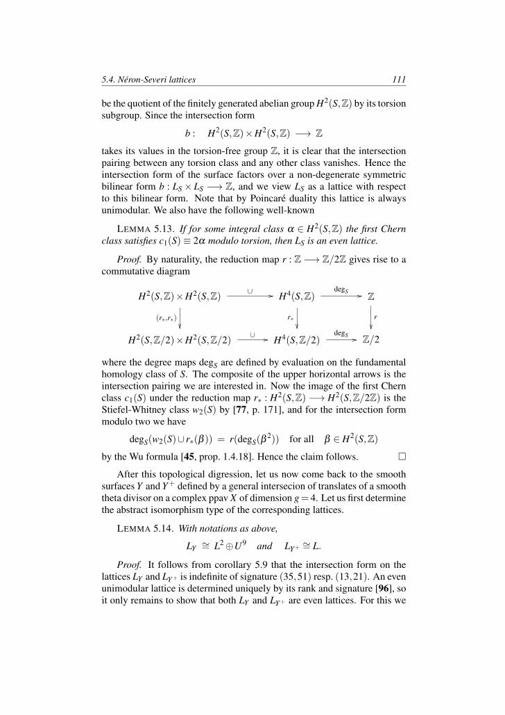
5.4. Neron-Severi lattices 111
be the quotient of the finitely generated abelian group H2(S,Z) by its torsionsubgroup. Since the intersection form
b : H2(S,Z)×H2(S,Z) −→ Z
takes its values in the torsion-free group Z, it is clear that the intersectionpairing between any torsion class and any other class vanishes. Hence theintersection form of the surface factors over a non-degenerate symmetricbilinear form b : LS× LS −→ Z, and we view LS as a lattice with respectto this bilinear form. Note that by Poincare duality this lattice is alwaysunimodular. We also have the following well-known
LEMMA 5.13. If for some integral class α ∈ H2(S,Z) the first Chernclass satisfies c1(S)≡ 2α modulo torsion, then LS is an even lattice.
Proof. By naturality, the reduction map r : Z −→ Z/2Z gives rise to acommutative diagram
H2(S,Z)×H2(S,Z) ∪ //
(r∗,r∗)
H4(S,Z)degS //
r∗
Z
r
H2(S,Z/2)×H2(S,Z/2) ∪ // H4(S,Z/2)degS // Z/2
where the degree maps degS are defined by evaluation on the fundamentalhomology class of S. The composite of the upper horizontal arrows is theintersection pairing we are interested in. Now the image of the first Chernclass c1(S) under the reduction map r∗ : H2(S,Z) −→ H2(S,Z/2Z) is theStiefel-Whitney class w2(S) by [77, p. 171], and for the intersection formmodulo two we have
degS(w2(S)∪ r∗(β )) = r(degS(β2)) for all β ∈ H2(S,Z)
by the Wu formula [45, prop. 1.4.18]. Hence the claim follows.
After this topological digression, let us now come back to the smoothsurfaces Y and Y+ defined by a general intersecion of translates of a smooththeta divisor on a complex ppav X of dimension g= 4. Let us first determinethe abstract isomorphism type of the corresponding lattices.
LEMMA 5.14. With notations as above,
LY ∼= L2⊕U9 and LY+ ∼= L.
Proof. It follows from corollary 5.9 that the intersection form on thelattices LY and LY+ is indefinite of signature (35,51) resp. (13,21). An evenunimodular lattice is determined uniquely by its rank and signature [96], soit only remains to show that both LY and LY+ are even lattices. For this we
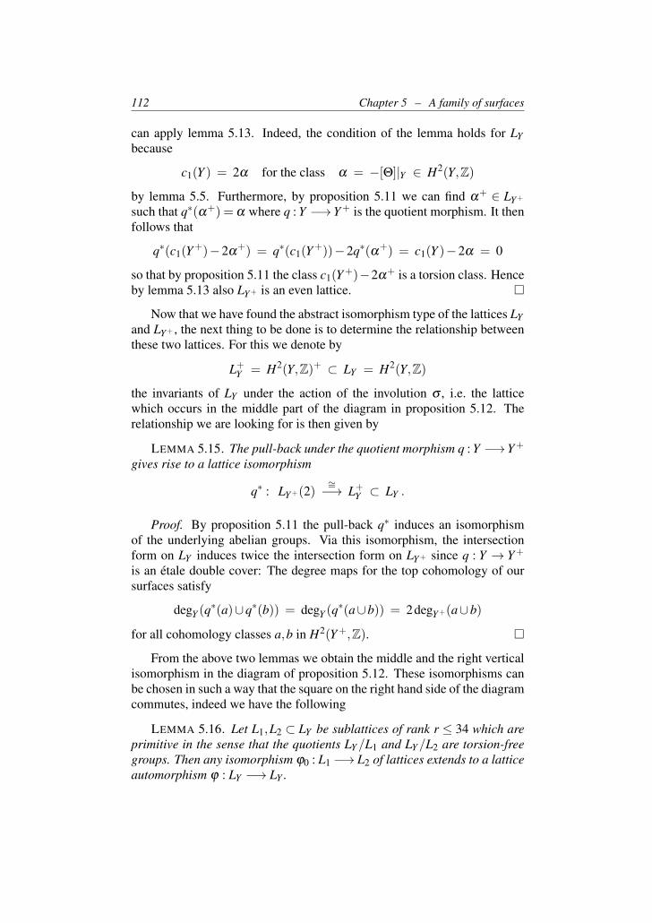
112 Chapter 5 – A family of surfaces
can apply lemma 5.13. Indeed, the condition of the lemma holds for LYbecause
c1(Y ) = 2α for the class α = −[Θ]|Y ∈ H2(Y,Z)
by lemma 5.5. Furthermore, by proposition 5.11 we can find α+ ∈ LY+
such that q∗(α+) = α where q : Y −→Y+ is the quotient morphism. It thenfollows that
q∗(c1(Y+)−2α+) = q∗(c1(Y+))−2q∗(α+) = c1(Y )−2α = 0
so that by proposition 5.11 the class c1(Y+)−2α+ is a torsion class. Henceby lemma 5.13 also LY+ is an even lattice.
Now that we have found the abstract isomorphism type of the lattices LYand LY+ , the next thing to be done is to determine the relationship betweenthese two lattices. For this we denote by
L+Y = H2(Y,Z)+ ⊂ LY = H2(Y,Z)
the invariants of LY under the action of the involution σ , i.e. the latticewhich occurs in the middle part of the diagram in proposition 5.12. Therelationship we are looking for is then given by
LEMMA 5.15. The pull-back under the quotient morphism q : Y −→Y+
gives rise to a lattice isomorphism
q∗ : LY+(2)∼=−→ L+
Y ⊂ LY .
Proof. By proposition 5.11 the pull-back q∗ induces an isomorphismof the underlying abelian groups. Via this isomorphism, the intersectionform on LY induces twice the intersection form on LY+ since q : Y → Y+
is an etale double cover: The degree maps for the top cohomology of oursurfaces satisfy
degY (q∗(a)∪q∗(b)) = degY (q
∗(a∪b)) = 2degY+(a∪b)
for all cohomology classes a,b in H2(Y+,Z).
From the above two lemmas we obtain the middle and the right verticalisomorphism in the diagram of proposition 5.12. These isomorphisms canbe chosen in such a way that the square on the right hand side of the diagramcommutes, indeed we have the following
LEMMA 5.16. Let L1,L2 ⊂ LY be sublattices of rank r ≤ 34 which areprimitive in the sense that the quotients LY/L1 and LY/L2 are torsion-freegroups. Then any isomorphism ϕ0 : L1 −→ L2 of lattices extends to a latticeautomorphism ϕ : LY −→ LY .
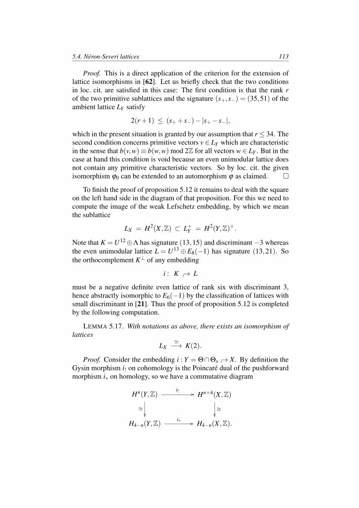
5.4. Neron-Severi lattices 113
Proof. This is a direct application of the criterion for the extension oflattice isomorphisms in [62]. Let us briefly check that the two conditionsin loc. cit. are satisfied in this case: The first condition is that the rank rof the two primitive sublattices and the signature (s+,s−) = (35,51) of theambient lattice LY satisfy
2(r+1) ≤ (s++ s−)−|s+− s−|,
which in the present situation is granted by our assumption that r≤ 34. Thesecond condition concerns primitive vectors v ∈ LY which are characteristicin the sense that b(v,w)≡ b(w,w) mod 2Z for all vectors w ∈ LY . But in thecase at hand this condition is void because an even unimodular lattice doesnot contain any primitive characteristic vectors. So by loc. cit. the givenisomorphism ϕ0 can be extended to an automorphism ϕ as claimed.
To finish the proof of proposition 5.12 it remains to deal with the squareon the left hand side in the diagram of that proposition. For this we need tocompute the image of the weak Lefschetz embedding, by which we meanthe sublattice
LX = H2(X ,Z) ⊂ L+Y = H2(Y,Z)+.
Note that K =U12⊕Λ has signature (13,15) and discriminant −3 whereasthe even unimodular lattice L = U13⊕E8(−1) has signature (13,21). Sothe orthocomplement K⊥ of any embedding
i : K → L
must be a negative definite even lattice of rank six with discriminant 3,hence abstractly isomorphic to E6(−1) by the classification of lattices withsmall discriminant in [21]. Thus the proof of proposition 5.12 is completedby the following computation.
LEMMA 5.17. With notations as above, there exists an isomorphism oflattices
LX∼=−→ K(2).
Proof. Consider the embedding i : Y = Θ∩Θx → X . By definition theGysin morphism i! on cohomology is the Poincare dual of the pushforwardmorphism i∗ on homology, so we have a commutative diagram
Hn(Y,Z)i! //
∼=
Hn+4(X ,Z)
∼=
H4−n(Y,Z)i∗ // H4−n(X ,Z).
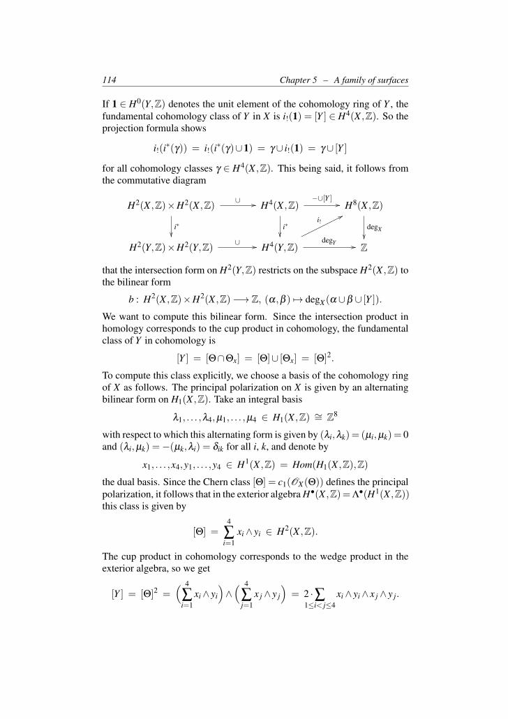
114 Chapter 5 – A family of surfaces
If 1 ∈ H0(Y,Z) denotes the unit element of the cohomology ring of Y , thefundamental cohomology class of Y in X is i!(1) = [Y ] ∈ H4(X ,Z). So theprojection formula shows
i!(i∗(γ)) = i!(i∗(γ)∪1) = γ ∪ i!(1) = γ ∪ [Y ]
for all cohomology classes γ ∈ H4(X ,Z). This being said, it follows fromthe commutative diagram
H2(X ,Z)×H2(X ,Z) ∪ //
i∗
H4(X ,Z)−∪[Y ]
//
i∗
H8(X ,Z)
degX
H2(Y,Z)×H2(Y,Z) ∪ // H4(Y,Z)degY //
i!77ooooooooooo
Z
that the intersection form on H2(Y,Z) restricts on the subspace H2(X ,Z) tothe bilinear form
b : H2(X ,Z)×H2(X ,Z)−→ Z, (α,β ) 7→ degX(α ∪β ∪ [Y ]).We want to compute this bilinear form. Since the intersection product inhomology corresponds to the cup product in cohomology, the fundamentalclass of Y in cohomology is
[Y ] = [Θ∩Θx] = [Θ]∪ [Θx] = [Θ]2.
To compute this class explicitly, we choose a basis of the cohomology ringof X as follows. The principal polarization on X is given by an alternatingbilinear form on H1(X ,Z). Take an integral basis
λ1, . . . ,λ4,µ1, . . . ,µ4 ∈ H1(X ,Z) ∼= Z8
with respect to which this alternating form is given by (λi,λk)= (µi,µk)= 0and (λi,µk) =−(µk,λi) = δik for all i, k, and denote by
x1, . . . ,x4,y1, . . . ,y4 ∈ H1(X ,Z) = Hom(H1(X ,Z),Z)
the dual basis. Since the Chern class [Θ] = c1(OX(Θ)) defines the principalpolarization, it follows that in the exterior algebra H•(X ,Z)=Λ•(H1(X ,Z))this class is given by
[Θ] =4
∑i=1
xi∧ yi ∈ H2(X ,Z).
The cup product in cohomology corresponds to the wedge product in theexterior algebra, so we get
[Y ] = [Θ]2 =( 4
∑i=1
xi∧ yi
)∧( 4
∑j=1
x j∧ y j
)= 2 ·∑
1≤i< j≤4xi∧ yi∧ x j∧ y j.
5.5. The upper bound W (E6) 115
In particular, it follows that v∧ [Y ] = 0 for all vectors v ∈ H4(X ,Z) of theform v = xk ∧ xl ∧ xm ∧ xn or v = xk ∧ xl ∧ xm ∧ yn or v = xk ∧ yl ∧ ym ∧ ynor v= yk∧yl∧ym∧yn with arbitrary indices k, l,m,n, and also for all vectorsof the form v = xk ∧ xl ∧ ym ∧ yn with k, l 6= m,n. However, for k 6= lone easily checks that
xk∧ xl ∧ yk∧ yl ∧ [Y ] = −2 ·ωfor the cohomology class
ω = x1∧ y1∧·· ·∧ x4∧ y4 = 14! · [Θ]4
mapped to 1 under the degree isomorphism degX : H8(X ,Z)−→ Z.
Now consider the basis of the lattice LX = Λ2(H1(X ,Z)) consisting ofthe vectors uik = xi∧yk with i,k ∈ 1,2,3,4 and of the vectors vik = xi∧xkand wik = yi ∧ yk with 1 ≤ i < k ≤ 4. It follows from the above that thebilinear form b is non-zero only on those pairs of the above vectors whosewedge product has the form ±xl ∧ xm ∧ yl ∧ ym with l 6= m. So the onlynon-zero scalar products between our basis vectors are
b(uii,ukk) = xi∧ yi∧ xk∧ yk∧ [Y ] = 2 for i 6= k,
b(uik,uki) = xi∧ yk∧ xk∧ yi∧ [Y ] =−2 for i 6= k, and
b(vik,wik) = b(wik,vik) = yi∧ yk∧ xi∧ xk∧ [Y ] =−2 for i < k.
Hence we obtain an orthogonal sum decomposition
LX = 〈u11, . . . ,u44〉 ⊕⊕
1≤i<k≤4
〈uik,uki〉⊕〈vik,wik〉
where 〈u11, . . . ,u44〉 ∼= Λ(2) and where 〈uik,uki〉 ∼= 〈vik,wik〉 ∼=U(2).
5.5. The upper bound W (E6)
Let us now come back to the local system which underlies the variationof Hodge structures V+ on the open dense subset U ⊂ X in lemma 5.10for g = 4, assuming that the theta divisor of our ppav is smooth. Sinceall constructions in the proof of that lemma make sense on the level ofintegral cohomology, we can in fact consider V+ as a polarized variationof Z-Hodge structures. Proposition 5.12 then allows to identify the fibresof this variation of Hodge structures with the lattice K⊥ ∼= E6(−1) up to arescaling of the bilinear form by a factor two.
This being said, consider the monodromy group G of the local systemunderlying V+. Since the monodromy action for any smooth proper familyof varieties preserves the intersection form on the cohomology of the fibres,it follows from the above that G must be contained in the automorphism
116 Chapter 5 – A family of surfaces
group Aut(E6) of the E6-lattice. Recall from [22, p. 126] that we have aproduct decomposition
Aut(E6) = W (E6)×±1where ±1 acts via multiplication by±1 on the E6-lattice. It turns out thatthe monodromy group G is already contained in the Weyl group itself.
PROPOSITION 5.18. With notations as above, the monodromy group Gis contained in the subgroup
W (E6) < Aut(E6).
Proof. Let K and L be as in proposition 5.12, and for some x ∈U(C)consider the monodromy operation of the group π1(U,x) on the σ -invariantlattice H2(Y,Z)+ ∼= L(2). Notice that on the sublattice H2(X ,Z) ∼= K(2)this monodromy operation is trivial. Dividing the bilinear forms by two, weobtain from proposition 5.12 an embedding
M = K⊕E6(−1) → L = U13⊕E8(−1)
with an action of the fundamental group π1(U,x) on L which is trivial onthe sublattice K and which preserves the orthocomplement E6(−1) = K⊥
on which it defines the quotient morphism
π1(U,x) G → Aut(E6)
we are interested in. We must show that the image G is already containedin the subgroup W (E6)< Aut(E6). To this end we will consider the inducedaction of G on the discriminant group of the E6-lattice.
Since the lattices L and M have the same rank, L is obtained from M byadjoining certain glue vectors, by which we mean as in [22] vectors fromthe dual lattice
M∗ =
m ∈M⊗ZQ | b(m,n) ∈ Z ∀n ∈M
= K∗⊕E6(−1)∗
where b denotes the bilinear form of the lattice M, extended to M⊗ZQ.Now the lattice E6(−1) has discriminant 3 whereas L is unimodular, sothere exists in the sublattice L⊆M∗=K∗⊕E6(−1)∗ at least one glue vectorof the form
λ = k+ e with k ∈ K∗, e ∈ E6(−1)∗ but e /∈ E6(−1).
Fixing k as above, consider the set S = f ∈ E6(−1)∗ | k+ f ∈ L. Thisset is stable under the monodromy operation, indeed this operation fixes kbecause H2(X ,Z) ∼= K(2) is contained in the monodromy invariant part ofthe cohomology. By construction S contains the coset e+E6(−1). On theother hand, for any f ∈ S we have
f − e = (k+ f )− (k+ e) ∈ E6(−1)∗∩L = E6(−1)
5.5. The upper bound W (E6) 117
where the last equality uses that E6(−1) = K⊥ is primitive in L, being theorthocomplement of a sublattice. Altogether then
S = e+E6(−1)
is a non-trivial coset of E6(−1) in E6(−1)∗ which is preserved by G. Sincethe discriminant group
E6(−1)∗/E6(−1) ∼= E∗6/E6 ∼= Z/3Zis generated by any non-trivial coset, it follows that G acts trivially onthis discriminant group. Now recall from [23, p. 27] that as a subgroupof Aut(E6) =W (E6)×±1 we have
W (E6) = ker(Aut(E6)−→ Aut(E∗6/E6)),
so the fact that the monodromy group G act trivially on the discriminantgroup implies that G≤W (E6) as required.
At this point let us briefly explain the connection of the above result withthe 27 Prym-embedded curves that have been studied by E. Izadi in [61],although this will not be used in the sequel. For the basic definitions andfacts about Prym varieties we refer to the brief survey in section 5.1 andto the references given there. Suppose that X is a general complex ppavof dimension g = 4. Then by [8, prop. 6.4] it can be written as the Prymvariety
X ∼= Prym(C/C)
for some etale double cover of smooth projective curves of genus 9 and 5,respectively. Consider then the covering involution ι : C→ C, and chooseany translate α : C → JC of the Abel-Jacobi map. Then the morphism
C −→ JC, p 7→ α(p)−α(ι(p))
factors over the kernel of the norm homomorphism NC/C : JC→ JC, hencethe image of some translate of this morphism is contained in the connectedcomponent
Prym(C/C) = (ker(NC/C))0
of the identity. Via the chosen isomorphism X ∼= Prym(C/C) this definesan embedding C → X which up to a translation is determined uniquely bythe etale double cover. Embeddings of this form are known as Abel-Prymembeddings, and by a Prym-embedded curve in X we mean the image ofany such embedding. Note that the etale double covering C→ C is by nomeans uniquely determined by the ppav X , indeed a dimension count showsthat the general fibre of the Prym morphism
π : R5 −→ A4
has dimension two. In studying this Prym morphism, E. Izadi has observedin [61, cor. 4.9] that for general x ∈ X(C), among all the Prym-embedded
118 Chapter 5 – A family of surfaces
curves precisely 27 are contained in the surface Y = Yx = Θ∩Θx. Thisnumber suggests a relationship with the E6-lattice in the cohomology of thissurface. Recall from [22] that the dual lattice E∗6 has precisely 27 pairs ofminimal vectors, with norm 4/3. It turns out that the fundamental classes ofPrym-embedded curves define such minimal vectors and are related to theglue vector λ = k+e∈ L with components k ∈K∗ and e∈ E6(−1)∗ that westudied in the proof of proposition 5.18.
LEMMA 5.19. The above glue vector λ = k+ e can be taken to be thefundamental class
[C ] ∈ H2(Y,Z)+ ∼= L(2)
of any Prym-embedded curve C⊂Y , and in this case the vector e∈E6(−1)∗
is a minimal vector with the norm b(e,e) =−4/3.
Proof. Any cohomology class λ ∈ H2(Y,Z)+ can be written uniquelyin the form
λ = α +β with α ∈ H2(X ,Q), β ∈ H2(X ,Q)⊥ ⊂ H2(Y,Q)+
and such a class defines a glue vector iff α /∈ H2(X ,Z). The integralityof α can be checked via the Gysin morphism for the embedding i : Y → Xsince i!(λ ) = α ∪ [Θ]2 ∈ H6(X ,Q) is the image of α under the Lefschetzisomorphism in the following commutative diagram.
H2(X ,Q)∼= //
i∗
''PPPPPPPH6(X ,Q)
H2(Y,Q)+
i! 77nnnnnnn
H2(X ,Z)
''PPPPPPP
?
OO
// H6(X ,Z)?
OO
H2(Y,Z)+
77nnnnnnn?
OO
Now by [13, sect. 12.2] the fundamental class λ = α +β ∈H2(Y,Q)+ of aPrym-embedded curve satisfies
α ∪ [Θ]2 = i!(λ ) = [Θ]3/3 /∈ H6(X ,Z)and hence indeed provides a glue vector for our lattices. It also follows fromthe above that
degY (α2) = degX(α
2∪ [Θ]2) = degX([Θ]4/9) = 8/3
where the last equality is due to the Poincare formula. Furthermore, bydefinition λ ∈ H2(Y,Q) is the class of a Prym-embedded curve C ⊂ Y and
5.6. Negligible constituents 119
any such curve has genus gC = 2g+1= 9. Hence the adjunction formula forthe genus of a smooth curve on a smooth projective surface [55, prop. V.1.5]gives the intersection number
degY (λ2) = 2gC−2−degY (KY |C) = 16−16 = 0,
indeed for the canonical class KY we have
degC(KY |C) = degY (λ ∪KY ) = degX(2 · [Θ]4/3) = 16
by the formula i!(λ ) = [Θ]3/3 from above and by lemma 5.5. We then alsoobtain the intersection number degY (β
2) = degY (λ2)−degY (α
2) =−8/3,and to see that the vector e is a minimal vector all that remains to be doneis to divide the bilinear form by two.
It seems a tempting idea to prove theorem 5.1 by looking directly at themonodromy operation on the fundamental classes of the Prym-embeddedcurves from above, but we have not seen how to do this. In what follows wegive a different proof which does not use the Prym construction, and fromthis point of view the theorem can be seen as an independent result aboutthe monodromy operation on the 27 Prym-embedded curves.
5.6. Negligible constituents
We now justify our earlier statement that for a general ppav the localsystems underlying the variations of Hodge structures V+ and V− fromlemma 5.10 are irreducible. In fact we will obtain stronger results since wewill work with perverse sheaves on the whole ppav rather than with localsystems on a Zariski-open dense subset. This shift in perspective reveals aclose connection with the Tannakian formalism of convolution as developedin chapters 2 and 3, which is of interest in its own right.
Recall that for any complex abelian variety X , the convolution producton the derived category Db
c (X ,C) of bounded complexes of C-sheaves withconstructible cohomology sheaves in the sense of [10] is defined by
K ∗L = Ra∗(KL) ∈ Dbc (X ,C) for K,L ∈ Db
c (X ,C),where a : X ×X −→ X denotes the group law. One of the main results ofchapter 2 was that the full abelian subcategory Perv(X ,C) ⊂ Db
c (X ,C) ofperverse sheaves is almost stable under the convolution product: Let us saythat a perverse sheaf is negligible if all its perverse subquotients have Eulercharacteristic zero; then theorem 2.13 shows that for all P,Q ∈ Perv(X ,C)and all n 6= 0 the perverse cohomology sheaves
pHn(X ,P∗Q) ∈ Perv(X ,C)are negligible. At the other end of the scale, we will say that a perversesheaf is clean if it does not have any negligible subquotients.
120 Chapter 5 – A family of surfaces
Suppose now that X has dimension g ≥ 2 and is principally polarizedwith a symmetric theta divisor Θ⊂X , and consider the perverse intersectioncohomology sheaf
δΘ = ICΘ[g−1] ∈ Perv(X ,C).
This is a semisimple perverse sheaf and arises via intermediate extensionfrom the constant sheaf on the smooth locus of the theta divisor. Thus wehave δΘ =CΘ[g−1] if the theta divisor is smooth, but later on we will alsodeal with isolated singularities.
LEMMA 5.20. If the theta divisor Θ has at most isolated singularities,then for every clean perverse sheaf P and all n ∈ Z, any simple negligiblesubquotient of pHn(δΘ ∗P) is isomorphic to δX = CX [g].
Proof. By Verdier duality it suffices to show this for n ≤ 0. Since thetheta divisor is a local complete intersection, by [65, lemma III.6.5] theshifted constant sheaf λΘ = CΘ[g− 1] is perverse, so we have an exactsequence of perverse sheaves
0−→ κ −→ λΘ −→ δΘ −→ 0
where κ is a skyscraper sheaf supported on the finite set of singular pointsof the theta divisor. Convolution with the clean perverse sheaf P yields adistinguished triangle
κ ∗P // λΘ ∗P // δΘ ∗P[+1]
// · · ·
where κ ∗ P is again a clean perverse sheaf. By the corresponding longexact sequence of perverse cohomology groups, it will therefore suffice toshow that every simple negligible subquotient of pHn(λΘ∗P) for n≤ 0 mustbe isomorphic to δX . But this follows as in [110, ex. 3] from the excisionsequence for the ample divisor Θ⊂ X with affine complement X \Θ, usingArtin’s vanishing theorem.
Let us now consider the convolution square δΘ ∗ δΘ. Due to Gabber’sdecomposition theorem this is a direct sum of degree shifts of semisimpleperverse sheaves. So we can write
δΘ ∗δΘ = S2(δΘ)⊕Λ2(δΘ)
where the symmetric square and the alternating square on the right hand sideare by definition the maximal direct summands on which the commutativityconstraint
S = SδΘ,δΘ: δΘ ∗δΘ −→ δΘ ∗δΘ
from section 2.1 acts by +1 resp. by −1. We want to relate the above sheafcomplexes to the variations of Hodge structures V± in lemma 5.10. In this
5.6. Negligible constituents 121
context, the contribution from the weak Lefschetz theorem will be describedby the complexes
L± =⊕µ∈ I±
Hg−2−|µ|(X ,C)⊗C δX [µ] with
I+ = 1+2Z,I− = 2Z,
where by convention H i(X ,C) = 0 for i < 0. Strictly speaking certain Tatetwists should be inserted in the above definition so that L± become purecomplexes of weight 2g− 2 like δΘ ∗ δΘ, but to keep the notations simplewe will in what follows suppress all occuring Tate twists.
LEMMA 5.21. If Θ has at most isolated singularities, then there aresemisimple perverse sheaves δ± ∈ Perv(X ,C) such that
S2(δΘ) ∼= L+⊕δ+ and Λ2(δΘ) ∼= L−⊕δ−,
and over the Zariski-open dense subset U ⊂ X from lemma 5.10 we have anisomorphism
δ±|U ∼= V±ε [g] with a sign twist by ε = (−1)g−1.
Proof. Consider the smooth proper family fU : YU −→U that we definedin lemma 5.3. By the construction in the proof of that lemma, we have acartesian diagram
YU = f−1(U) //
fU
Θsm×Θsm // Θ×Θ
f
U // X
where Θsm ⊆ Θ is the smooth locus of the theta divisor and where f isinduced by the group law. From the definition of convolution we thereforeobtain natural identifications
(δΘ ∗δΘ)|U ∼= (CΘ[g−1]∗CΘ[g−1])|U ∼= R fU∗(CYU [2g−2]).
By Gabber’s decomposition theorem this is a direct sum of degree shifts ofsemisimple perverse sheaves, hence
(δΘ ∗δΘ)|U ∼=2g−4⊕n=0
Hn[2g−2−n]
for the local systems Hn = Rn fU∗(CYU ) with stalks Hnx = Hn(Yx,C). In
the proof of lemma 5.10 we have observed that these local systems containconstant subsheaves whose stalks are the subspaces which are the imagesof the restriction morphisms Hn(X ,C) −→ Hn(Yx,C). This being said, weobtain that
(δΘ ∗δΘ)|U = (L+⊕L−)|U ⊕V[g]
122 Chapter 5 – A family of surfaces
where V = V+⊕V− denotes the local system underlying the variations ofHodge structures in lemma 5.10. Via Gabber’s decomposition theorem onethen deduces that
δΘ ∗δΘ = L+⊕L−⊕δ for some δ ∈ Dbc (X ,C).
But we know from theorem 2.13 that for all n 6= 0 the perverse cohomologysheaves pHn(δΘ ∗δΘ) are negligible and are hence by lemma 5.20 multiplesof the constant perverse sheaf δX . Since over the open dense subset U ⊂ Xwe have δ |U = V[g], it then follows that δ is a perverse sheaf.
Now consider the direct sum decomposition δ = δ+⊕δ− where δ± ⊂ δ
are defined as the maximal perverse subsheaves on which the commutativityconstraint S : δΘ ∗δΘ −→ δΘ ∗δΘ acts by±1. Going back to the definitions,one checks that this commutativity constraint S induces on the stalks theinvolution ε ·σ∗x : Hn(Yx,Q)−→Hn(Yx,Q) where σx : Yx −→Yx denotes theinvolution that we defined in section 5.2 and where the twist by the extrasign ε = (−1)g−1 comes from the degree shift in δΘ = ICΘ[g−1] becauseof the Koszul rule for the tensor product of complexes.
Recall that a perverse sheaf is said to be clean if it does not admit anyperverse subquotients which are negligible. For a smooth theta divisor weclaim that L± are the only negligible constituents in δΘ ∗δΘ.
LEMMA 5.22. If the theta divisor Θ⊂ X is smooth, then δ± are clean.
Proof. If this were not true, then by lemma 5.20 the semisimple perversesheaf δ+⊕δ− would contain δX as a summand. Then H−g(X ,δ+⊕δ−) 6= 0and hence the inclusion
H−g(X ,L+⊕L−) → H−g(X ,δΘ ∗δΘ)
would be strict. However, the Kunneth formula in lemma 3.4 and the weakLefschetz theorem for the smooth ample divisor Θ⊂ X show that
H−g(X ,δΘ ∗δΘ) =g−1⊕n=1
H−n(X ,δΘ)⊗Hn−g(X ,δΘ)
=g−1⊕n=1
Hg−1−n(X ,C)⊗Hn−1(X ,C)
which by direct inspection is equal to H−g(X ,L+⊕L−).
Note that for a general complex ppav of dimension g the theta divisoris smooth by the work of Andreotti and Mayer [4], so the above lemmatogether with theorem 4.2 leads to the final result of this section.
PROPOSITION 5.23. If X is a general complex ppav of dimension g,then the local systems underlying V± are irreducible.
5.7. Jacobian varieties 123
Proof. For a general ppav we know from theorem 4.2 that the Tannakagroup G(δΘ) is either a symplectic or a special orthogonal group and thatthe perverse intersection cohomology sheaf δΘ corresponds to the standardrepresentation of this group. Now the symmetric and alternating square ofthe standard representation are irreducible up to a trivial one-dimensionalrepresentation, and this trivial representation corresponds to the skyscrapersheaf δ0 of rank one supported in the origin. Furthermore, by corollary 2.9each representation of the Tannaka group corresponds to a unique cleanperverse sheaf. Hence from lemma 5.22 we obtain that there exist cleanand simple perverse sheaves γ± ∈ Perv(X ,C) such that
δ+ =
γ+⊕δ0
γ+and δ− =
γ−γ−⊕δ0
if g is
odd,even,
and by lemma 5.21 the simplicity of γ± in particular implies that the localsystems V± are irreducible.
5.7. Jacobian varieties
Let us now see what happens if X = JC is the Jacobian variety of asmooth complex projective curve C of genus g≥ 2. To formulate our resultsin this case we first need to introduce some more notations. For n ∈ N wewill denote by
Cn = (C×·· ·×C)/Sn
the n-fold symmetric product of the curve and by Wn ⊂ X the image of Cnunder a suitable translate of the Abel-Jacobi map, normalized such that thetheta divisor Θ = Wg−1 becomes symmetric. We write fn : Cn −→Wn forthe Abel-Jacobi map and gn : Wn×Wn −→ X for the difference morphismwith gn(x,y) = y− x. Then the composite morphism
Cn×Cn( fn, fn) //
dn
77Wn×Wn
gn // X ∼= Pic0(C)
does not depend on the chosen normalization of the Abel-Jacobi map, and itsends a pair (D,E) ∈Cn×Cn of effective divisors of degree n on the curveto the isomorphism class of the line bundle OC(D−E).
In what follows we will be especially interested in non-hyperellipticcurves of genus g = 4. For these we know from lemma 4.5 that the thetadivisor has only isolated singularities, so we can consider the variations ofHodge structures V± from lemma 5.10 and the perverse sheaves δ± fromlemma 5.21. Here we have the following situation.
124 Chapter 5 – A family of surfaces
PROPOSITION 5.24. Let X = JC be the Jacobian variety of a smoothnon-hyperelliptic complex projective curve C of genus g = 4.
(a) The above semisimple perverse sheaves δ+ and δ− each containthe negligible constituent δX precisely once.
(b) After shrinking the open dense subset U ⊂ X in lemma 5.10 thereexists an isomorphism
V+∼= d2∗(CC2×C2)|U .
Proof. (a) We must check for the lowest hypercohomology degree thatdim(H−g(X ,δ+)) = dim(H−g(X ,δ−)) = 1. For this we can use the samecomputation as in lemma 5.22, the only difference is that for a Jacobianvariety the hypercohomology H•(X ,δΘ) is larger than the one for a generalppav. Indeed it has been shown in [106, cor. 13(iii)] that if the curve C isnot hyperelliptic, then
H i(X ,δΘ) =
H i+3(X ,C) for i ∈ −3,−2,H i+3(X ,C)⊕H i+1(X ,C) for i ∈ −1,0.
Compared with the computation in lemma 5.22, for i =−1 the extra directsummand H0(X ,C)⊂ H−1(X ,δΘ) gives a two-dimensional extra term
H0(X ,C)⊗H−3(X ,δΘ) ⊕ H−3(X ,δΘ)⊗H0(X ,C) ⊂ H−4(X ,δΘ ∗δΘ).
This extra term splits into two one-dimensional contributions, one in thesymmetric and one in the alternating tensor square. Hence
H−4(X ,S2(δΘ)) = H−4(X ,L+)⊕C,
H−4(X ,Λ2(δΘ)) = H−4(X ,L−)⊕C,
and our claim follows because S2(δΘ) = L+⊕δ+ and Λ2(δΘ) = L−⊕δ−.
(b) This is most conveniently checked in the setting of Brill-Noethersheaves and will be done after the proof of lemma 5.25 below.
Before we proceed further, let us recall from [106] some facts aboutBrill-Noether sheaves. Here we are mainly interested in their Tannakiandescription — more about their geometric construction can be found in thebrief survey in section 6.1 below. Let X = JC be the Jacobian variety of asmooth non-hyperelliptic complex projective curve C of genus g ≥ 2, andlet C → X be a translate of the Abel-Jacobi map such that the correspondingtheta divisor Θ =Wg−1 is symmetric. Then by loc. cit. the convolutions ofthe perverse intersection cohomology sheaf δC ∈ Perv(X ,C) are describedvia corollary 2.14 by the Tannaka group
G(δC) = Sl2g−2(C).
5.7. Jacobian varieties 125
For partitions α = (α1,α2, . . .) such that 2g− 2 ≥ α1 ≥ α2 ≥ ·· · ≥ 0, onecan define the Brill-Noether sheaf
pδ α ∈ Perv(X ,C)
as the simple perverse sheaf corresponding to the irreducible representationof Sl2g−2(C) whose highest weight is given by the conjugate partition α t
in the basis of the weights defined by the diagonal entries of matrices. Forinstance, the singleton partitions α = (α1) correspond to the fundamentalrepresentations, and for these it has been shown in loc. cit. that
pδ i ∼= δWi and p
δ 2g−2−i ∼= δ−Wi for 0≤ i≤ g−1,
where the second equality is due to the Riemann-Roch theorem. Now theTannakian formalism provides a means to decompose arbitrary convolutionproducts between these perverse intersection cohomology sheaves via thecombinatorial Littlewood-Richardson rule for the decomposition of tensorproducts of irreducible representations of Sl2g−2(C), see [46, sect. 9.3.5]and [106, sect. 5.4]. In the special case of fundamental representations thisgives the formula
pδ m ∗ p
δ n ∼= τm,n ⊕n⊕
i=0
pδ (m+i,n−i) for m≥ n,
where τm,n ∈ Dbc (X ,C) is a negligible sheaf complex in the sense that all
its perverse cohomology sheaves have Euler characteristic zero. In fact ithas been shown in lemma 27 of loc. cit. that τm,n (and more generally anynegligible direct summand of a convolution of Brill-Noether sheaves) is adirect sum of degree shifts of δX = CX [g]. As an application we have thefollowing result concerning the difference morphism.
LEMMA 5.25. Let X = JC be the Jacobian variety of a non-hyperellipticsmooth projective curve of even genus g= 2n. Then over some Zariski-opendense subset U ⊂ X there exists an irreducible local system LU of complexvector spaces such that
dn∗(CCn×Cn)|U ∼= CU ⊕LU .
Proof. A Bertini-type argument like the one in lemma 5.3 shows thatover some Zariski-open dense subset U ⊂ X the morphism dn restricts to afinite etale cover. Furthermore, if S denotes the singular locus of Wn, thenfor dimension reasons the closed subset (S×Wn)∪ (Wn× S) ⊂Wn×Wn ismapped under the difference morphism
gn : Wn×Wn −→ X
to a proper closed subset of X , so we can assume that g−1n (U) is contained
in (Wn\S)×(Wn\S). The Riemann-Kempf singularity theorem [48, p. 348]
126 Chapter 5 – A family of surfaces
says that the Abel-Jacobi morphism fn : Cn−→Wn restricts over the smoothlocus to an isomorphism
f−1n (Wn \S)
∼=−→ Wn \S.
Putting everything together and using the commutative diagram
Cn×Cn( fn, fn) //
dn
..
Wn×Wn
gn
(−in,in) // X×X
a
ppX
for the closed embedding in : Wn → X , we therefore obtain by the definitionof convolution an isomorphism
dn∗(CCn×Cn[g])|U ∼= (δWn ∗δ−Wn)|U .
To control the convolution on the right hand side, we use the formalism ofBrill-Noether sheaves. Recall that δWn =
pδ n and δ−Wn =pδ 3n−2, where the
second equality is due to the Riemann-Roch theorem. Hence we get fromthe Littlewood-Richardson rule that
δWn ∗δ−Wn∼= p
δ n ∗ pδ 3n−2 ∼= τ ⊕
n⊕i=0
pδ 3n−2+i,n−i
where τ is a direct sum of degree shifts of δX . In fact τ = δX as one may seefrom the above isomorphism dn∗(CCn×Cn[g])|U ∼= (δWn ∗ δ−Wn)|U and fromthe fact that dn is generically finite. Therefore our claim will follow for thecohomology sheaf
LU = H −g(pδ 3n−2,n)|U ,
provided that for all i > 0 the perverse sheaves pδ 3n−2+i,n−i are supportedon a proper closed subset of X . But this is indeed the case because by theLittlewood-Richardson rule the perverse sheaf
n⊕i=1
pδ 3n−2+i,n−i ∼= p
δ n−1 ∗ pδ 2g−(n−1)
∼= δWn−1 ∗δ−Wn−1
has the support dn−1(Cn−1×Cn−1)⊂ X of dimension 2(n−1)< g.
Proof of part (b) in proposition 5.24. For this we again use Brill-Noethersheaves. The perverse sheaf δΘ = δW3 =
pδ 3 corresponds by definition tothe third fundamental representation of the Tannaka group Sl6(C). One cancheck that the alternating square of this representation decomposes into twoirreducible pieces of highest weight α t for α = (4,2) and α = (6). Henceit follows that
δ− ∼= pδ 4,2⊕ p
δ 6⊕ τ
5.8. The difference morphism 127
where τ ∈ Perv(X ,C) is some negligible perverse sheaf. In fact τ = δX bypart (a) of the proposition. Furthermore pδ 6 = δ0 is a skyscraper sheaf,hence for U ⊂ X sufficiently small we have
V+∼= H −4(δ−)|U ∼= H −4(p
δ 4,2⊕δX)|U ∼= d2∗(CC2×C2)
where the first isomorphism is due to lemma 5.21 and where the last onecomes from the proof of lemma 5.25 for n = 2.
5.8. The difference morphism
Motivated by the previous section, let C be a smooth complex projectivecurve of genus g = 2n with n ∈ N, and put
Cn = (C×·· ·×C)/Sn.
We want to study the difference morphism dn : Cn×Cn −→ X = JC fromabove. To begin with, we claim that this morphism is generically finite andhas generic degree
N = deg(dn) =(2n
n
).
Indeed, by birationality of the Abel-Jacobi map Cn→Wn it suffices to checkthat the difference morphism gn : Wn×Wn→ X is generically finite of thegiven degree. Note that the fibre of gn over a point x ∈ X(C) is isomorphicto the intersection Z =Wn∩ (Wn+x). Now a Bertini-type argument and thePoincare formula [13, sect. 11.2.1] for the fundamental classes
[Wn] = [Wn + x] = 1n! · [Θ]n ∈ Hn(X ,Z)
show that for a sufficiently general point x∈X(C) the intersection Z is finiteof cardinality
|Z| = degX([Wn]∪ [Wn + x]
)= g!
n!·n! = N.
So over some Zariski-open dense subset U ⊂ X the morphisms gn and dnrestrict to a finite etale cover of degree N as claimed.
Now pick x ∈ U(C), and consider the monodromy action of π1(U,x)on the N distinct points of the fibre d−1
n (x). Labelling these points in anychosen order, we get a homomorphism
π1(U,x) −→ SN
to the symmetric group, and we define the monodromy group G(dn) tobe the image of this homomorphism. A different choice of the labellingonly changes this subgroup by an inner automorphism of Sn. Our goal isto determine the monodromy group G(dn) for a general curve C of evengenus g = 2n. For this we will study a degeneration into a hyperellipticcurve, where we have the following situation.
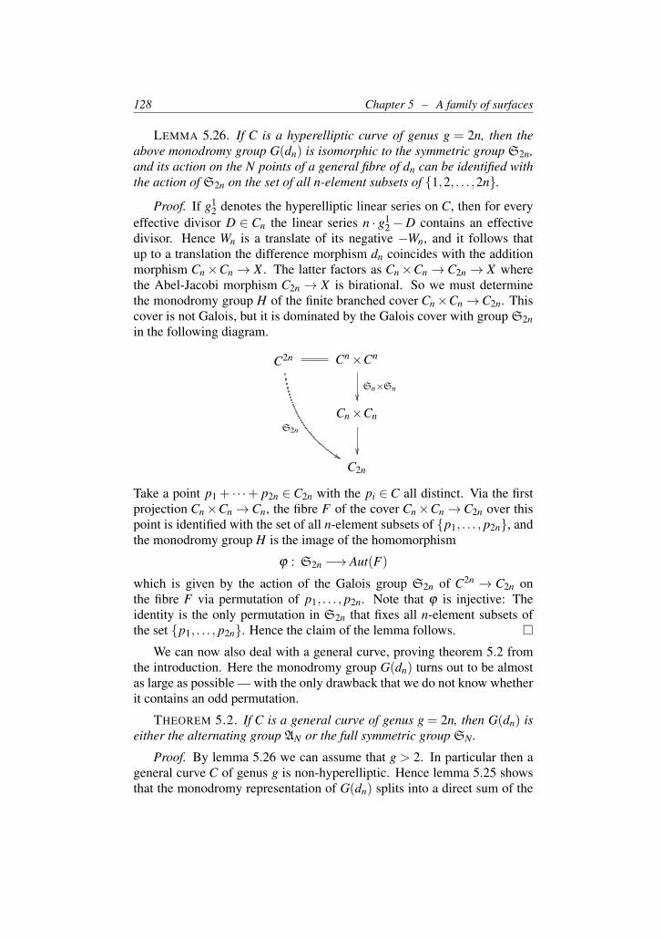
128 Chapter 5 – A family of surfaces
LEMMA 5.26. If C is a hyperelliptic curve of genus g = 2n, then theabove monodromy group G(dn) is isomorphic to the symmetric group S2n,and its action on the N points of a general fibre of dn can be identified withthe action of S2n on the set of all n-element subsets of 1,2, . . . ,2n.
Proof. If g12 denotes the hyperelliptic linear series on C, then for every
effective divisor D ∈ Cn the linear series n · g12−D contains an effective
divisor. Hence Wn is a translate of its negative −Wn, and it follows thatup to a translation the difference morphism dn coincides with the additionmorphism Cn×Cn → X . The latter factors as Cn×Cn → C2n → X wherethe Abel-Jacobi morphism C2n → X is birational. So we must determinethe monodromy group H of the finite branched cover Cn×Cn→C2n. Thiscover is not Galois, but it is dominated by the Galois cover with group S2nin the following diagram.
C2n
S2n
%%
Cn×Cn
Sn×Sn
Cn×Cn
C2n
Take a point p1 + · · ·+ p2n ∈C2n with the pi ∈C all distinct. Via the firstprojection Cn×Cn→Cn, the fibre F of the cover Cn×Cn→C2n over thispoint is identified with the set of all n-element subsets of p1, . . . , p2n, andthe monodromy group H is the image of the homomorphism
ϕ : S2n −→ Aut(F)
which is given by the action of the Galois group S2n of C2n → C2n onthe fibre F via permutation of p1, . . . , p2n. Note that ϕ is injective: Theidentity is the only permutation in S2n that fixes all n-element subsets ofthe set p1, . . . , p2n. Hence the claim of the lemma follows.
We can now also deal with a general curve, proving theorem 5.2 fromthe introduction. Here the monodromy group G(dn) turns out to be almostas large as possible — with the only drawback that we do not know whetherit contains an odd permutation.
THEOREM 5.2. If C is a general curve of genus g = 2n, then G(dn) iseither the alternating group AN or the full symmetric group SN .
Proof. By lemma 5.26 we can assume that g > 2. In particular then ageneral curve C of genus g is non-hyperelliptic. Hence lemma 5.25 showsthat the monodromy representation of G(dn) splits into a direct sum of the
5.8. The difference morphism 129
one-dimensional trivial representation plus only a single further irreduciblerepresentation. Now recall that by definition G(dn) is a subgroup of thesymmetric group SN . If V = CN denotes the permutation representationof SN , then the monodromy representation of the subgroup G(dn) is simplythe restriction of V to this subgroup. Note that V = 1⊕W splits as thedirect sum of the one-dimensional trivial representation plus an irreduciblerepresentation W of SN with dimension N−1. In these terms, the remarksat the beginning of the proof amount to the statement that the restrictionof W to the subgroup G(dn)≤SN remains irreducible.
It is a general fact from the theory of permutation groups [91, th. 1(b)]that any subgroup of SN with this irreducibility property is a 2-transitivesubgroup. So by lemma D.1 in the appendix it will suffice to show that for ageneral curve C of genus g = 2n the monodromy group G(dn) contains thehyperelliptic one from lemma 5.26. For this we consider a degeneration ofa general curve into a hyperelliptic curve.
Let p : C → S be a flat, projective family of smooth curves of genus gover a smooth quasi-projective complex base curve S, and assume that thefibre Cs = p−1(s) is hyperelliptic for some special point s = s0 ∈ S(C) butnon-hyperelliptic for all s 6= s0. The existence of such families followse.g. from [5, th. XII.9.1]. To rephrase our previous constructions in thisrelative setting, let X be the relative Picard scheme of C over S as definedin [15, sect. 8.2], and denote by Cn = (C ×S · · ·×S C )/Sn the n-th relativesymmetric product. Let L be a Poincare bundle on C ×S×Cn so that forall s ∈ S(C) and every divisor D ∈ Cn,s(C) we have L |Cs×D
∼= OCs(D).If p1, p2 : C ×S Cn×S Cn → C ×S Cn denote the projections, then by theuniversal property of the Picard scheme the line bundle p∗1(L )⊗ p∗2(L
−1)determines a morphism dn : Cn×S Cn→X which on the fibres over eachpoint s ∈ S(C) restricts to the difference morphism from above.
This being said, take an open subset U ⊆X over which dn is finite etaleof degree N and such that over every point s ∈ S(C) the fibre Us =U ∩Xsis dense in Xs. Applying the semicontinuity lemma 5.27 below to the localsystem L = dn∗(CCn×SCn)|U , we obtain that the monodromy group of dnfor a general curve of genus g = 2n contains the hyperelliptic one fromlemma 5.26 as a subgroup. This finishes the proof.
For the above degeneration argument we have made use of the followingsemicontinuity property for monodromy groups in families. Let f : U → Sbe a smooth morphism of complex algebraic varieties whose target is aquasi-projective curve S, and consider a local system L of complex vectorspaces on U with finite monodromy group. For any point u ∈U(C) withimage s = f (u) we denote by
G(u) = Im(π1(Us,u) −→ AutC(Lu)
)
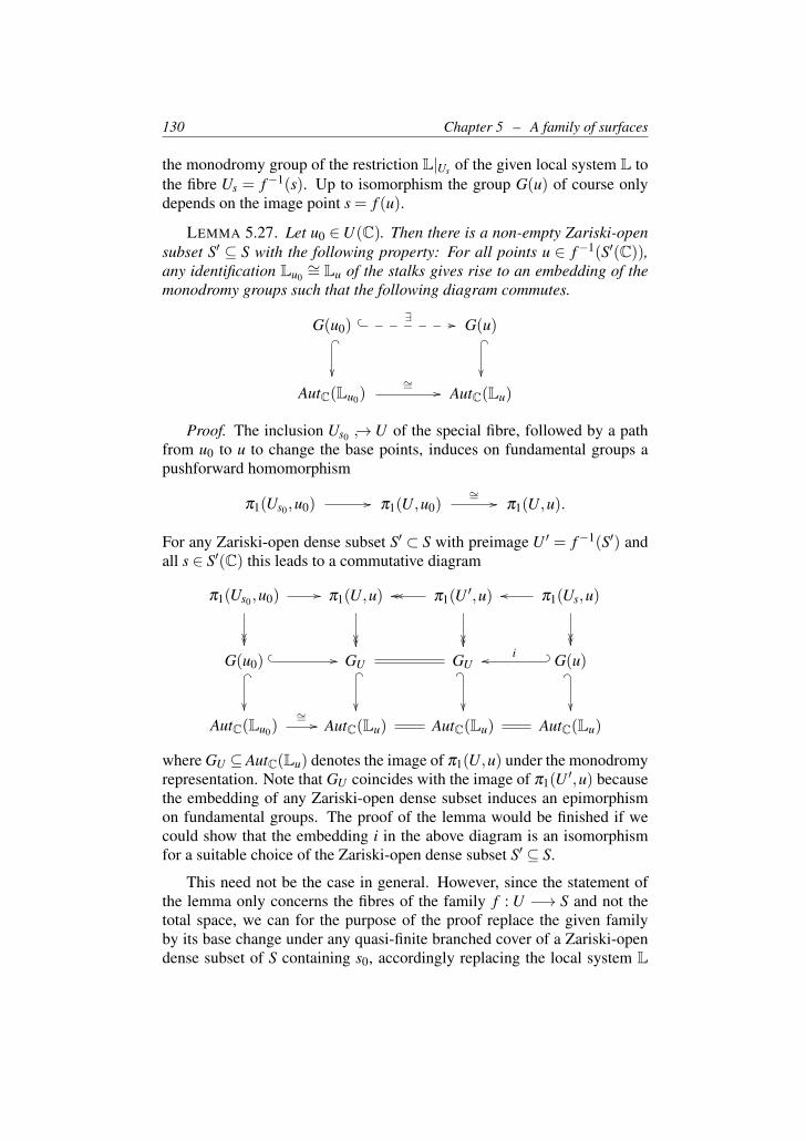
130 Chapter 5 – A family of surfaces
the monodromy group of the restriction L|Us of the given local system L tothe fibre Us = f−1(s). Up to isomorphism the group G(u) of course onlydepends on the image point s = f (u).
LEMMA 5.27. Let u0 ∈U(C). Then there is a non-empty Zariski-opensubset S′ ⊆ S with the following property: For all points u ∈ f−1(S′(C)),any identification Lu0
∼= Lu of the stalks gives rise to an embedding of themonodromy groups such that the following diagram commutes.
G(u0) ∃ //_______
_
G(u) _
AutC(Lu0)∼= // AutC(Lu)
Proof. The inclusion Us0 →U of the special fibre, followed by a pathfrom u0 to u to change the base points, induces on fundamental groups apushforward homomorphism
π1(Us0,u0) // π1(U,u0)∼= // π1(U,u).
For any Zariski-open dense subset S′ ⊂ S with preimage U ′ = f−1(S′) andall s ∈ S′(C) this leads to a commutative diagram
π1(Us0 ,u0) //
π1(U,u)
π1(U ′,u)oooo
π1(Us,u)oo
G(u0) //
_
GU _
GU_
G(u)? _ioo_
AutC(Lu0)∼= // AutC(Lu) AutC(Lu) AutC(Lu)
where GU ⊆ AutC(Lu) denotes the image of π1(U,u) under the monodromyrepresentation. Note that GU coincides with the image of π1(U ′,u) becausethe embedding of any Zariski-open dense subset induces an epimorphismon fundamental groups. The proof of the lemma would be finished if wecould show that the embedding i in the above diagram is an isomorphismfor a suitable choice of the Zariski-open dense subset S′ ⊆ S.
This need not be the case in general. However, since the statement ofthe lemma only concerns the fibres of the family f : U −→ S and not thetotal space, we can for the purpose of the proof replace the given familyby its base change under any quasi-finite branched cover of a Zariski-opendense subset of S containing s0, accordingly replacing the local system L
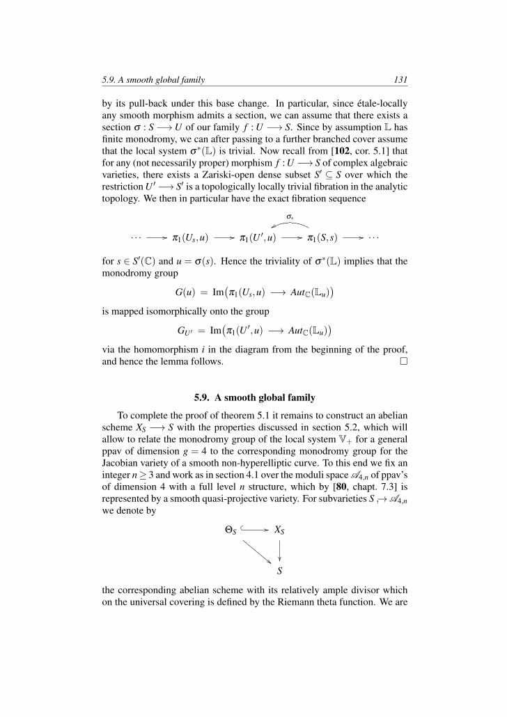
5.9. A smooth global family 131
by its pull-back under this base change. In particular, since etale-locallyany smooth morphism admits a section, we can assume that there exists asection σ : S −→U of our family f : U −→ S. Since by assumption L hasfinite monodromy, we can after passing to a further branched cover assumethat the local system σ∗(L) is trivial. Now recall from [102, cor. 5.1] thatfor any (not necessarily proper) morphism f : U −→ S of complex algebraicvarieties, there exists a Zariski-open dense subset S′ ⊆ S over which therestriction U ′−→ S′ is a topologically locally trivial fibration in the analytictopology. We then in particular have the exact fibration sequence
· · · // π1(Us,u) // π1(U ′,u) // π1(S,s) //
σ∗xx
· · ·
for s ∈ S′(C) and u = σ(s). Hence the triviality of σ∗(L) implies that themonodromy group
G(u) = Im(π1(Us,u) −→ AutC(Lu)
)is mapped isomorphically onto the group
GU ′ = Im(π1(U ′,u) −→ AutC(Lu)
)via the homomorphism i in the diagram from the beginning of the proof,and hence the lemma follows.
5.9. A smooth global family
To complete the proof of theorem 5.1 it remains to construct an abelianscheme XS −→ S with the properties discussed in section 5.2, which willallow to relate the monodromy group of the local system V+ for a generalppav of dimension g = 4 to the corresponding monodromy group for theJacobian variety of a smooth non-hyperelliptic curve. To this end we fix aninteger n≥ 3 and work as in section 4.1 over the moduli space A4,n of ppav’sof dimension 4 with a full level n structure, which by [80, chapt. 7.3] isrepresented by a smooth quasi-projective variety. For subvarieties S →A4,nwe denote by
ΘS //
""DDD
DDDD
DDXS
S
the corresponding abelian scheme with its relatively ample divisor whichon the universal covering is defined by the Riemann theta function. We are
132 Chapter 5 – A family of surfaces
interested in the composite morphism
f : YS = ΘS×S ΘS // XS×S XS
a // XS
where a denotes the group law of the abelian scheme. For each s ∈ S(C)the restriction f |Xs : f−1(Xs) −→ Xs is the family of the intersections oftranslates of the theta divisor for the corresponding ppav Xs as in the proofof the Bertini-type lemma 5.3.
LEMMA 5.28. There exists a smooth quasi-projective curve S ⊂ A4,nwith the following properties.
(a) For some s0 ∈ S(C) the fibre Xs0 is the Jacobian variety of a generalcurve, whereas for all other points s 6= s0 the theta divisor Θs ⊂ Xsis smooth.
(b) The family f : YS −→ S of intersecting theta divisors restricts to asmooth proper morphism
f |US : f−1(US) −→ US
over some Zariski-open subset US ⊂ XS which surjects onto S.
Proof. The locus of all ppav’s with a singular theta divisor is itselfa divisor in the moduli space A4,n, and it contains the locus of Jacobianvarieties as a component [4]. Hence if we take S → A4,n to be a smoothquasi-projective complex curve which meets the locus of Jacobian varietiesin a general point s0 ∈ S(C) and is otherwise contained in the Zariski-opendense locus of ppav’s with a smooth theta divisor, then (a) holds.
Consider then the corresponding morphism f :YS−→XS. By the genericflatness theorem in the form of lemma 5.29 below, we find a Zariski-opendense subset US ⊂ XS which maps surjectively onto S and furthermore hasthe property that the restriction
f |US : f−1(US) −→ US
is a flat morphism. Now recall from lemma 4.5 that the theta divisor of thenon-hyperelliptic Jacobian variety Xs0 has only isolated singularities, so bythe Bertini-type lemma 5.3 we can find a point u in Us0 = US ∩Xs0 suchthat the fibre Yu = f−1(u) is smooth. Furthermore, for any proper and flatmorphism of varieties over a field which has at least one smooth fibre, thereexists by [55, ex. III.10.2] a non-empty Zariski-open subset of the targetover which the morphism is smooth. In our case therefore f restricts toa smooth morphism over some Zariski-open neighborhood of the point uin US. We can replace US by such a neighborhood and accordingly shrinkthe curve S in such a way that the special point s0 still lies in S(C) but thatnow also the properties in claim (b) are satisfied.
5.9. A smooth global family 133
For the sake of completeness we include the following version of thegeneric flatness theorem that has been used in the above lemma.
LEMMA 5.29. Let V and W be two integral schemes which are locallyof finite type over a locally Noetherian, integral, regular base scheme S ofdimension one. Suppose that for every point s in S the scheme-theoreticfibre Vs is non-empty and Ws is reduced. Let
Vf //
AAA
AAA W
||||
||
S
be an S-morphism of finite type. Then the flat locus
US = w ∈W | f is flat at v for all v ∈V with f (v) = wis a Zariski-open dense subset of W which maps surjectively onto S.
Proof. Since V and W are integral schemes which dominate the integralregular one-dimensional scheme S, they are automatically flat over S in viewof [55, prop. III.9.7]. So the fibre-wise flatness criterion [50, th. 11.3.10]shows that the morphism f is flat over a point w in W if and only if therestriction fs : Vs→Ws to the scheme-theoretic fibres over the image s ∈ Sof w is flat over w. Now the generic flatness theorem [49, th. 6.9.1] applieson the one hand to the finite type morphism f : V →W and on the otherhand to its restriction fs : Vs→Ws. Since by assumption both W and Ws areintegral, it follows that the flat locus US is on the one hand a Zariski-opendense subset of W and on the other hand meets every fibre Ws.

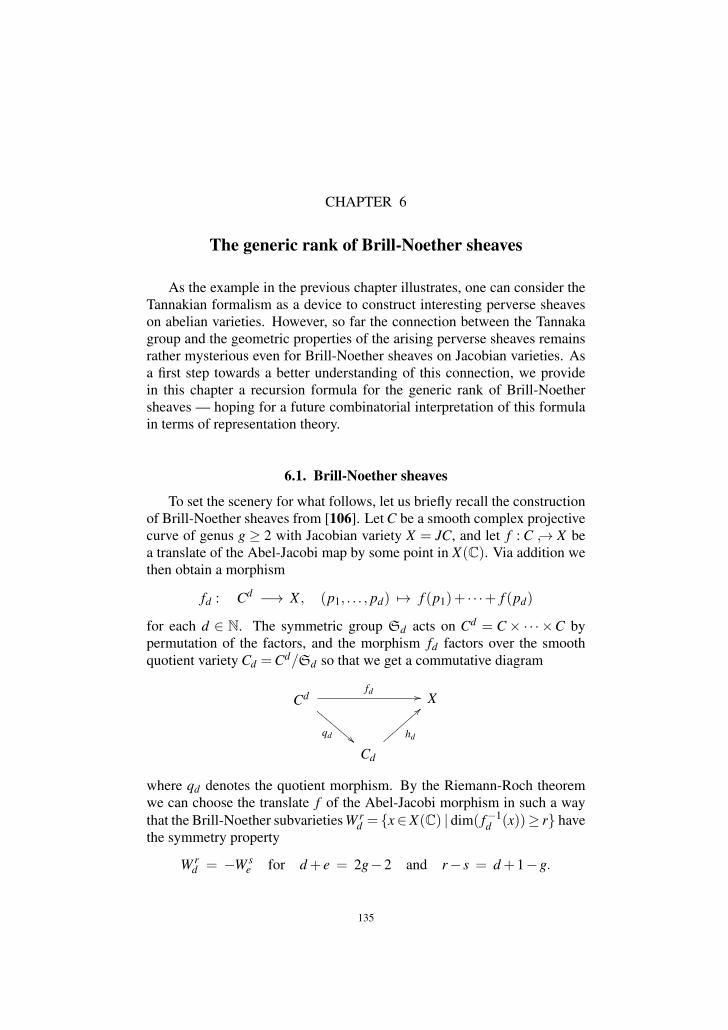
CHAPTER 6
The generic rank of Brill-Noether sheaves
As the example in the previous chapter illustrates, one can consider theTannakian formalism as a device to construct interesting perverse sheaveson abelian varieties. However, so far the connection between the Tannakagroup and the geometric properties of the arising perverse sheaves remainsrather mysterious even for Brill-Noether sheaves on Jacobian varieties. Asa first step towards a better understanding of this connection, we providein this chapter a recursion formula for the generic rank of Brill-Noethersheaves — hoping for a future combinatorial interpretation of this formulain terms of representation theory.
6.1. Brill-Noether sheaves
To set the scenery for what follows, let us briefly recall the constructionof Brill-Noether sheaves from [106]. Let C be a smooth complex projectivecurve of genus g ≥ 2 with Jacobian variety X = JC, and let f : C → X bea translate of the Abel-Jacobi map by some point in X(C). Via addition wethen obtain a morphism
fd : Cd −→ X , (p1, . . . , pd) 7→ f (p1)+ · · ·+ f (pd)
for each d ∈ N. The symmetric group Sd acts on Cd = C× ·· · ×C bypermutation of the factors, and the morphism fd factors over the smoothquotient variety Cd =Cd/Sd so that we get a commutative diagram
Cdfd //
qd !!DDD
DDDD
DX
Cd
hd
==
where qd denotes the quotient morphism. By the Riemann-Roch theoremwe can choose the translate f of the Abel-Jacobi morphism in such a waythat the Brill-Noether subvarieties W r
d = x∈X(C) | dim( f−1d (x))≥ r have
the symmetry property
W rd = −W s
e for d + e = 2g−2 and r− s = d +1−g.
135
136 Chapter 6 – The generic rank of Brill-Noether sheaves
With these normalizations, the following explicit description has beengiven in loc. cit. for the Tannakian category generated by the convolutionpowers of the perverse sheaf δC = δW1 ∈ Perv(X ,C). A complete set ofirreducible representations of the symmetric group Sd up to isomorphismis given by the Specht modules σα where α runs through the partitions ofdegree d, see [88]. So the direct image of the constant perverse sheaf underthe branched Galois cover qd : Cd −→Cd splits up under the action of Sdas a direct sum
qd∗(δCd) =⊕
deg(α)=d
σα γα with certain γα ∈ Perv(Cd,C).
Consider now the direct image complexes δα = Rhd∗(γα). Each of these isa retract of R fd∗(δCd) = δC ∗ · · · ∗ δC as one easily checks from the abovedecomposition. By theorem 10 in loc. cit. we can write
δα = pδ α ⊕ c
δ α
where pδ α is a semisimple perverse sheaf without constituents of Eulercharacteristic zero and where the sheaf complex cδ α is a sum of degreeshifts of the constant perverse sheaf δX = CX [g]. In particular, cδ α is themaximal direct summand of δα which lies in the full subcategory T(X)of negligible objects from section 3.3. One can show that pδ α 6= 0 iff thepartition α = (d1, . . . ,dn) satisfies d1 ≤ 2g− 2. Let us call such partitionsadmissible. The constituents of the perverse sheaves pδ α for the admissiblepartitions α are called Brill-Noether sheaves. They are the simple objectsof the Tannakian category generated by δC in the sense of corollary 3.10,and by loc. cit. the corresponding Tannaka group is
G(δC) =
Sp2g−2(C) if C is hyperelliptic,Sl2g−2(C) otherwise.
If the curve C is not hyperelliptic, then for any admissible partition α it turnsout that the perverse sheaf pδ α corresponds to the irreducible representationof Sl2g−2(C) whose highest weight is given by the conjugate partition α t
in the basis defined by the diagonal entries of matrices. For example, thefundamental representations of Sl2g−2(C) correspond to partitions α = (d)with a single part, and for these one has
pδ d =
δWd for 0≤ d ≤ g−1,δ−W2g−2−d for g≤ d ≤ 2g−2.
A similar interpretation holds in the hyperelliptic case, but here the pδ α
are in general no longer irreducible; their decomposition is obtained byapplying the restriction functor from representations of the group Sl2g−2(C)to representations of the subgroup Sp2g−2(C).
6.2. A formula for the generic rank 137
6.2. A formula for the generic rank
The main goal of the present chapter is to obtain a recursive formulafor the generic rank rα of the perverse sheaves pδ α , by which we moreprecisely mean the rank
rα = dimC(H −g(p
δ α)η
)of the lowest degree cohomology sheaf at the generic point η ∈ X . Notethat rα = 0 if and only if the perverse sheaf pδ α is supported on a properclosed subset of X (indeed any simple perverse sheaf arises via intermediateextension from a local system on an open dense subset of its support).
THEOREM 6.1. For partitions α = (d1, . . . ,dn) of degree d = deg(α)the generic rank rα is given by the recursion
rα = ∑c1+···+cn=g
0≤ci≤di
[ g!c1!···cn! −1
] n
∏k=1
(2(g−1−ck)dk−ck
)− ∑
β>α
deg(β )=d
Kβα · rβ .
where the Kβα are the Kostka numbers defined combinatorially below.
Here we use the following conventions: For any integers a,m ∈ Z thebinomial coefficient
(ma
)is defined as the coefficient of ta in the expansion
of (1+ t)m as a power series, hence it vanishes for a < 0 and is given forexponents m < 0 by the formula
(ma
)= (−1)a ·
(a−m−1a
). For partitions α
and β the notation β > α refers to the lexicographic ordering. Finally, werecall that the Kostka numbers Kβα are non-negative integers which can bedefined combinatorially in the following way.
By a Young diagram of shape β = (e1, . . . ,em) we mean a diagram of mleft-aligned rows such that for each i the ith row consists of ei cells. If thecells of the diagram are filled with the entries 1,2, . . . ,n and each entry joccurs precisely d j times, the resulting array is called a Young tableau ofcontent α = (d1, . . . ,dn). A Young tableau is said to be semistandard if theentries of the rows are weakly increasing from left to right and those of thecolumns are strictly increasing from top to bottom; by definition the Kostkanumber Kβα is the number of such tableaux of shape β and content α . Forexample, we have K(3,2),(2,2,1) = 2 since
1 1 22 3
1 1 32 2
are the only semistandard tableaux of shape (3,2) and content (2,2,1). Theabove definition also easily implies that the Kostka numbers satisfy Kαα = 1and Kβα = 0 for all partitions β < α .
138 Chapter 6 – The generic rank of Brill-Noether sheaves
The Kostka numbers arise in the representation theory of the symmetricgroup: Young’s rule [88, th. 2.11.2] says that for partitions α = (d1, . . . ,dn)of degree d = deg(α) we have
(?) IndSdSd1×···×Sdn
(1) =⊕β≥α
Kβα ·σβ
where the left hand side denotes the representation induced from the trivialrepresentation 1 of the subgroup Sd1×·· ·×Sdn ≤Sd . Since Kαα = 1, itfollows that the dimensions of the Specht modules satisfy
(??) dim(σα) = d!d1!···dn! − ∑
β>α
Kβα ·dim(σβ ).
This being said, let us take a look at the recursion formula in theorem 6.1 insome explicit examples.
EXAMPLE 6.2. Let α be a partition of degree d. For d < g the first sumin theorem 6.1 is empty so that rα = 0. More interestingly, in degree d = gthe recursion of the theorem says
rα = g!d1!···dn! − 1 − ∑
β>α
Kβα · rβ
which together with (??) implies
rα =
dim(σα) if α 6= (g),0 if α = (g).
We remark that this can also be checked directly as follows. For d < gthe subvariety Wd is a proper closed subset of X , and by construction itcontains the support of pδ α . Similarly, in degree d = g the Abel-Jacobimorphism hd : Cd→ X is birational, and in this case our claim follows fromthe observation that the perverse sheaf γα ∈ Perv(Cd,C) from section 6.1has generic rank dim(σα) and contains the constant perverse sheaf if andonly if α = (g) is a singleton partition. However, for partitions of higherdegree the situation becomes increasingly complicated.
EXAMPLE 6.3. For g = 4 theorem 6.1 predicts that r6 = r5,1 = 0 andmore interestingly that
r4,2 = [ 4!2!·2! −1] ·
(22
)·(2
0
)= 5,
r3,3 = 2 · [ 4!3!·1! −1] ·
(00
)·(4
2
)+[ 4!
2!·2! −1] ·(2
1
)·(2
1
)− r4,2 = 51.
6.3. Computations in the symmetric product 139
In this case the vanishing r6 = r5,1 = 0 can again be checked directly,using the observation that
pδ 6⊕ p
δ 5,1 = pδ 1 ∗ p
δ 5 = δW1 ∗δ−W1
must be supported on the two-dimensional closed subset W1−W1 ⊂ X . Thevalues r4,2 = 5 and r3,3 = 51 are less obvious from a geometric point ofview, but notice that they are one less than the generic ranks of the localsystems V± in chapter 5, in accordance with part (b) of proposition 5.24.
More numerical values for partitions of small degree can be found insection 6.6 below. After these examples, let us now come to the proof ofthe recursion formula in theorem 6.1. Consider the stalk cohomology of theconvolution product δ α = δd1 ∗· · ·∗δdn . For each i∈1,2, . . . ,n the Spechtmodule σdi is the trivial representation of the symmetric group Sdi , hence itfollows from equation (?) above and from the construction of Brill-Noethersheaves in section 6.1 that
δα =
⊕β≥α
Kβα ·δβ = pδ
α ⊕ cδ
α
where
pδ
α =⊕β≥α
Kβα · pδ β and cδ
α =⊕β≥α
Kβα · cδ β .
The stalk cohomology of a perverse sheaf at a general point x ∈ X(C) isconcentrated in degree −g, so to prove theorem 6.1 we can replace thegeneric rank by (−1)g times the Euler characteristic of the generic stalkcohomology. Thus it will suffice to show that for general x ∈ X(C),
∑m∈Z
(−1)m+g dimC(Hm(δ α)x) = ∑
c1,...,cn≥0c1+···+cn=g
g!c1!···cn!
n
∏k=1
(2(g−1−ck)dk−ck
),
∑m∈Z
(−1)m+g dimC(Hm(c
δα)x) = ∑
c1,...,cn≥0c1+···+cn=g
n
∏k=1
(2(g−1−ck)dk−ck
).
The first of these equalities will follow from theorem 6.6 below since bybase change H •(δ α)x is equal to the cohomology of the fibre F = f−1
α (x)of the Abel-Jacobi morphism fα : Cd1×·· ·×Cdn→ X . The second equalityrests on a computation of Betti polynomials, see corollary 6.8.
6.3. Computations in the symmetric product
In this section we compute some intersection numbers of cycle classesin the cohomology ring of the symmetric products of C that will be neededin the proof of theorem 6.6 below. For d ∈ N consider the Abel-Jacobimorphism hd : Cd → X = JC as before. We will always work with rational
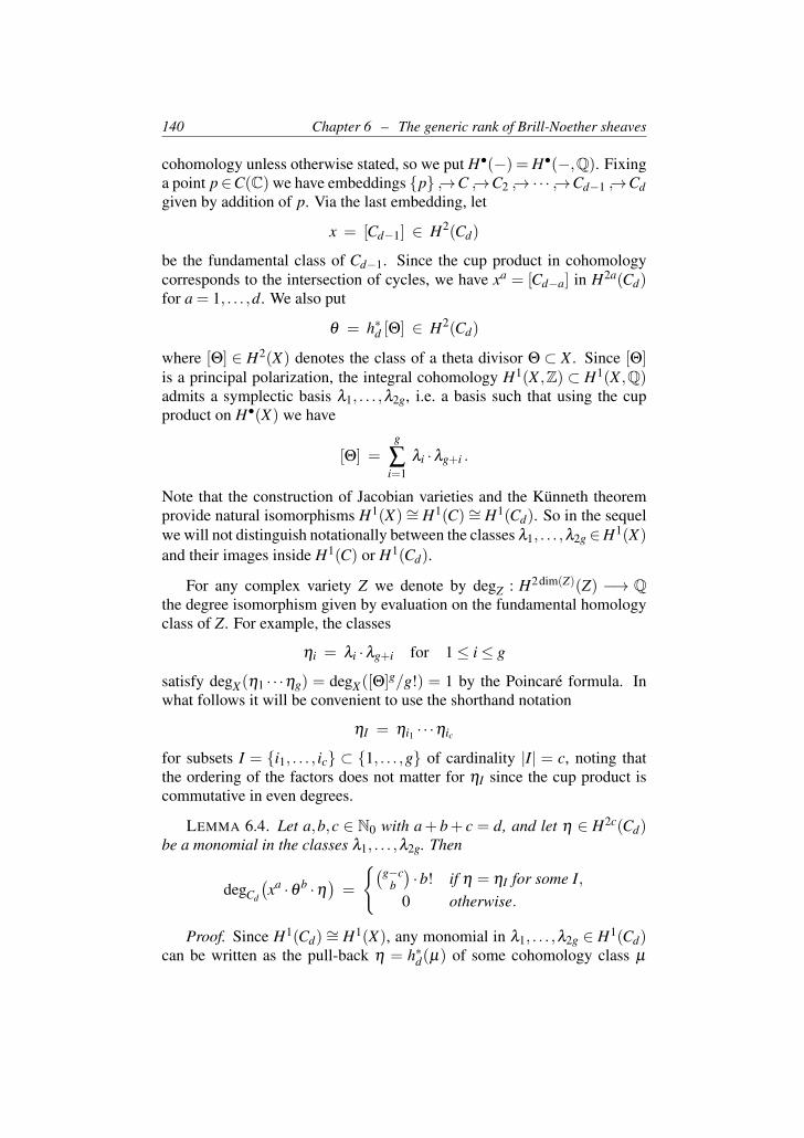
140 Chapter 6 – The generic rank of Brill-Noether sheaves
cohomology unless otherwise stated, so we put H•(−) = H•(−,Q). Fixinga point p∈C(C) we have embeddings p →C →C2 →·· · →Cd−1 →Cdgiven by addition of p. Via the last embedding, let
x = [Cd−1] ∈ H2(Cd)
be the fundamental class of Cd−1. Since the cup product in cohomologycorresponds to the intersection of cycles, we have xa = [Cd−a] in H2a(Cd)for a = 1, . . . ,d. We also put
θ = h∗d [Θ] ∈ H2(Cd)
where [Θ] ∈ H2(X) denotes the class of a theta divisor Θ ⊂ X . Since [Θ]is a principal polarization, the integral cohomology H1(X ,Z) ⊂ H1(X ,Q)admits a symplectic basis λ1, . . . ,λ2g, i.e. a basis such that using the cupproduct on H•(X) we have
[Θ] =g
∑i=1
λi ·λg+i .
Note that the construction of Jacobian varieties and the Kunneth theoremprovide natural isomorphisms H1(X)∼= H1(C)∼= H1(Cd). So in the sequelwe will not distinguish notationally between the classes λ1, . . . ,λ2g ∈H1(X)
and their images inside H1(C) or H1(Cd).
For any complex variety Z we denote by degZ : H2dim(Z)(Z) −→ Qthe degree isomorphism given by evaluation on the fundamental homologyclass of Z. For example, the classes
ηi = λi ·λg+i for 1≤ i≤ g
satisfy degX(η1 · · ·ηg) = degX([Θ]g/g!) = 1 by the Poincare formula. Inwhat follows it will be convenient to use the shorthand notation
ηI = ηi1 · · ·ηic
for subsets I = i1, . . . , ic ⊂ 1, . . . ,g of cardinality |I| = c, noting thatthe ordering of the factors does not matter for ηI since the cup product iscommutative in even degrees.
LEMMA 6.4. Let a,b,c ∈ N0 with a+ b+ c = d, and let η ∈ H2c(Cd)be a monomial in the classes λ1, . . . ,λ2g. Then
degCd
(xa ·θ b ·η
)=
(g−cb
)·b! if η = ηI for some I,
0 otherwise.
Proof. Since H1(Cd) ∼= H1(X), any monomial in λ1, . . . ,λ2g ∈ H1(Cd)can be written as the pull-back η = h∗d(µ) of some cohomology class µ
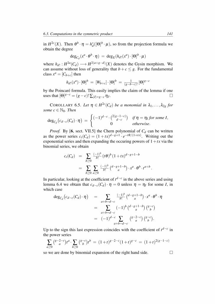
6.3. Computations in the symmetric product 141
in H2c(X). Then θ b ·η = h∗d([Θ]b · µ), so from the projection formula weobtain the degree
degCd(xa ·θ b ·η) = degX(hd!(xa) · [Θ]b ·µ)
where hd! : H2a(Cd) −→ H2(a+g−d)(X) denotes the Gysin morphism. Wecan assume without loss of generality that b+ c ≤ g. For the fundamentalclass xa = [Cb+c] then
hd!(xa) · [Θ]b = [Wb+c] · [Θ]b = 1(g−b−c)! [Θ]g−c
by the Poincare formula. This easily implies the claim of the lemma if oneuses that [Θ]g−c = (g− c)!∑|J|=g−c ηJ .
COROLLARY 6.5. Let η ∈ H2c(Cd) be a monomial in λ1, . . . ,λ2g forsome c ∈ N0. Then
degCd
(cd−c(Cd) ·η
)=
(−1)d−c ·
(2(g−1−c)d−c
)if η = ηI for some I,
0 otherwise.
Proof. By [6, sect. VII.5] the Chern polynomial of Cd can be writtenas the power series ct(Cd) = (1+ tx)d−g+1 · e−tθ/(1+tx). Writing out theexponential series and then expanding the occuring powers of 1+ tx via thebinomial series, we obtain
ct(Cd) = ∑b≥0
(−1)b
b! (tθ)b (1+ tx)d−g+1−b
= ∑b≥0
∑a≥0
(−1)b
b!
(d−g+1−ba
)· xa ·θ b · ta+b .
In particular, looking at the coefficient of td−c in the above series and usinglemma 6.4 we obtain that cd−c(Cd) ·η = 0 unless η = ηI for some I, inwhich case
degCd
(cd−c(Cd) ·η
)= ∑
a+b=d−c
(−1)b
b!
(d−g+1−ba
)· xa ·θ b ·η
= ∑a+b=d−c
(−1)b (d−g+1−ba
)(g−cb
)= (−1)d−c
∑a+b=d−c
(g−2−ca
)(g−cb
).
Up to the sign this last expression coincides with the coefficient of td−c inthe power series
∑a≥0
(g−2−ca
)ta ·∑
b≥0
(g−cb
)tb = (1+ t)g−2−c(1+ t)g−c = (1+ t)2(g−1−c)
so we are done by binomial expansion of the right hand side.
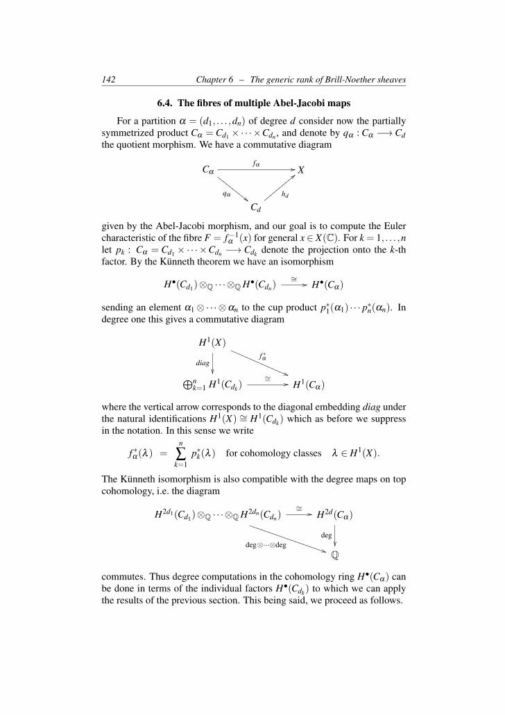
142 Chapter 6 – The generic rank of Brill-Noether sheaves
6.4. The fibres of multiple Abel-Jacobi maps
For a partition α = (d1, . . . ,dn) of degree d consider now the partiallysymmetrized product Cα = Cd1 ×·· ·×Cdn , and denote by qα : Cα −→ Cdthe quotient morphism. We have a commutative diagram
Cα
fα //
qα""F
FFFF
FFFF
F X
Cd
hd
<<zzzzzzzzzz
given by the Abel-Jacobi morphism, and our goal is to compute the Eulercharacteristic of the fibre F = f−1
α (x) for general x ∈ X(C). For k = 1, . . . ,nlet pk : Cα = Cd1 × ·· · ×Cdn −→ Cdk denote the projection onto the k-thfactor. By the Kunneth theorem we have an isomorphism
H•(Cd1)⊗Q · · ·⊗Q H•(Cdn)∼= // H•(Cα)
sending an element α1⊗ ·· ·⊗αn to the cup product p∗1(α1) · · · p∗n(αn). Indegree one this gives a commutative diagram
H1(X)f ∗α
((QQQQQQQQQQQQQQQ
diag⊕n
k=1 H1(Cdk)∼= // H1(Cα)
where the vertical arrow corresponds to the diagonal embedding diag underthe natural identifications H1(X) ∼= H1(Cdk) which as before we suppressin the notation. In this sense we write
f ∗α(λ ) =n
∑k=1
p∗k(λ ) for cohomology classes λ ∈ H1(X).
The Kunneth isomorphism is also compatible with the degree maps on topcohomology, i.e. the diagram
H2d1(Cd1)⊗Q · · ·⊗Q H2dn(Cdn)
deg⊗···⊗deg))TTTTTTTTTTTTTTTTTTTT
∼= // H2d(Cα)
deg
Q
commutes. Thus degree computations in the cohomology ring H•(Cα) canbe done in terms of the individual factors H•(Cdk) to which we can applythe results of the previous section. This being said, we proceed as follows.
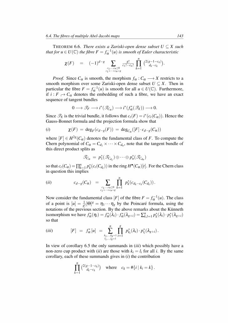
6.4. The fibres of multiple Abel-Jacobi maps 143
THEOREM 6.6. There exists a Zariski-open dense subset U ⊆ X suchthat for u ∈U(C) the fibre F = f−1
α (u) is smooth of Euler characteristic
χ(F) = (−1)d−g∑
c1,...,cn≥0c1+···+cn=g
g!c1!···cn!
n
∏k=1
(2(g−1−ck)dk−ck
).
Proof. Since Cα is smooth, the morphism fα : Cα −→ X restricts to asmooth morphism over some Zariski-open dense subset U ⊆ X . Then inparticular the fibre F = f−1
α (u) is smooth for all u ∈U(C). Furthermore,if i : F → Cα denotes the embedding of such a fibre, we have an exactsequence of tangent bundles
0−→TF −→ i∗(TCα)−→ i∗( f ∗α(TX))−→ 0.
Since TX is the trivial bundle, it follows that ct(F) = i∗(ct(Cα)). Hence theGauss-Bonnet formula and the projection formula show that
(i) χ(F) = degF(cd−g(F)) = degCα([F ] · cd−g(Cα))
where [F ] ∈ H2g(Cα) denotes the fundamental class of F . To compute theChern polynomial of Cα = Cd1 ×·· ·×Cdn , note that the tangent bundle ofthis direct product splits as
TCα= p∗1(TCd1
)⊕·· ·⊕ p∗n(TCdn)
so that ct(Cα)=∏nk=1 p∗k(ct(Cdk)) in the ring H•(Cα)[t]. For the Chern class
in question this implies
(ii) cd−g(Cα) = ∑c1,...,cn≥0
c1+···+cn=g
n
∏k=1
p∗k(cdk−ck(Cdk)) .
Now consider the fundamental class [F ] of the fibre F = f−1α (u). The class
of a point is [u] = 1g! [Θ]g = η1 · · ·ηg by the Poincare formula, using the
notations of the previous section. By the above remarks about the Kunnethisomorphism we have f ∗α(ηi) = f ∗α(λi) · f ∗α(λg+i) = ∑
nk,l=1 p∗k(λi) · p∗l (λg+i)
so that
(iii) [F ] = f ∗α [u] =n
∑k1,...,kg=1l1,...,lg=1
g
∏i=1
p∗ki(λi) · p∗li(λg+i) .
In view of corollary 6.5 the only summands in (iii) which possibly have anon-zero cup product with (ii) are those with ki = li for all i. By the samecorollary, each of these summands gives in (i) the contribution
n
∏k=1
(2(g−1−ck)dk−ck
)where ck = #i | ki = k .
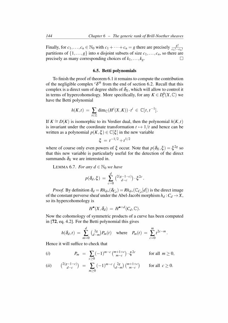
144 Chapter 6 – The generic rank of Brill-Noether sheaves
Finally, for c1, . . . ,cn ∈ N0 with c1 + · · ·+ cn = g there are precisely g!c1!···cn!
partitions of 1, . . . ,g into n disjoint subsets of size c1, . . . ,cn, so there areprecisely as many corresponding choices of k1, . . . ,kg.
6.5. Betti polynomials
To finish the proof of theorem 6.1 it remains to compute the contributionof the negligible complex cδ
α from the end of section 6.2. Recall that thiscomplex is a direct sum of degree shifts of δX , which will allow to control itin terms of hypercohomology. More specifically, for any K ∈ Db
c (X ,C) wehave the Betti polynomial
h(K, t) = ∑i∈Z
dimC(H i(X ,K)) · t i ∈ C[ t, t−1].
If K ∼= D(K) is isomorphic to its Verdier dual, then the polynomial h(K, t)is invariant under the coordinate transformation t 7→ 1/t and hence can bewritten as a polynomial p(K,ξ ) ∈ C[ξ ] in the new variable
ξ = t−1/2 + t1/2
where of course only even powers of ξ occur. Note that p(δX ,ξ ) = ξ 2g sothat this new variable is particularly useful for the detection of the directsummands δX we are interested in.
LEMMA 6.7. For any d ∈ N0 we have
p(δd,ξ ) =d
∑c=0
(2(g−1−c)d−c
)·ξ 2c .
Proof. By definition δd = Rhd∗(δCd) = Rhd∗(CCd [d]) is the direct imageof the constant perverse sheaf under the Abel-Jacobi morphism hd : Cd→X ,so its hypercohomology is
H•(X ,δd) = H•+d(Cd,C).Now the cohomology of symmetric products of a curve has been computedin [72, eq. 4.2]. For the Betti polynomial this gives
h(δd, t) =d
∑m=0
( 2gd−m
)Pm(t) where Pm(t) =
m
∑c=0
t2c−m .
Hence it will suffice to check that
Pm = ∑c≥0
(−1)m−c (m+1+cm−c
)·ξ 2c for all m≥ 0,(i) (2(g−1−c)
d−c
)= ∑
m≥0(−1)m−c ( 2g
d−m
)(m+1+cm−c
)for all c≥ 0.(ii)
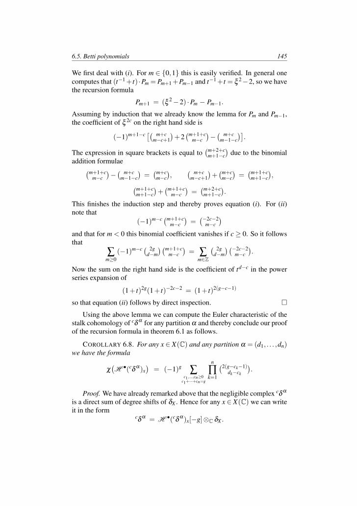
6.5. Betti polynomials 145
We first deal with (i). For m ∈ 0,1 this is easily verified. In general onecomputes that (t−1+ t) ·Pm = Pm+1+Pm−1 and t−1+ t = ξ 2−2, so we havethe recursion formula
Pm+1 = (ξ 2−2) ·Pm − Pm−1.
Assuming by induction that we already know the lemma for Pm and Pm−1,the coefficient of ξ 2c on the right hand side is
(−1)m+1−c [( m+cm−c+1
)+2(m+1+c
m−c
)−( m+c
m−1−c
)].
The expression in square brackets is equal to(m+2+c
m+1−c
)due to the binomial
addition formulae(m+1+cm−c
)−( m+c
m−1−c
)=(m+c
m−c
),
( m+cm−c+1
)+(m+c
m−c
)=(m+1+c
m+1−c
),(m+1+c
m+1−c
)+(m+1+c
m−c
)=(m+2+c
m+1−c
).
This finishes the induction step and thereby proves equation (i). For (ii)note that
(−1)m−c (m+1+cm−c
)=(−2c−2
m−c
)and that for m < 0 this binomial coefficient vanishes if c≥ 0. So it followsthat
∑m≥0
(−1)m−c ( 2gd−m
)(m+1+cm−c
)= ∑
m∈Z
( 2gd−m
)(−2c−2m−c
).
Now the sum on the right hand side is the coefficient of td−c in the powerseries expansion of
(1+ t)2g(1+ t)−2c−2 = (1+ t)2(g−c−1)
so that equation (ii) follows by direct inspection.
Using the above lemma we can compute the Euler characteristic of thestalk cohomology of cδ
α for any partition α and thereby conclude our proofof the recursion formula in theorem 6.1 as follows.
COROLLARY 6.8. For any x ∈ X(C) and any partition α = (d1, . . . ,dn)we have the formula
χ(H •(c
δα)x)
= (−1)g∑
c1,...,cn≥0c1+···+cn=g
n
∏k=1
(2(g−ck−1)dk−ck
).
Proof. We have already remarked above that the negligible complex cδα
is a direct sum of degree shifts of δX . Hence for any x ∈ X(C) we can writeit in the form
cδ
α = H •(cδ
α)x[−g]⊗C δX .
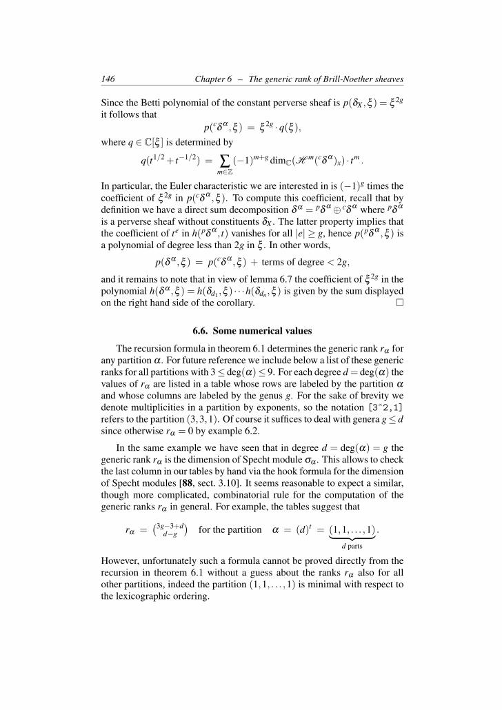
146 Chapter 6 – The generic rank of Brill-Noether sheaves
Since the Betti polynomial of the constant perverse sheaf is p(δX ,ξ ) = ξ 2g
it follows thatp(c
δα ,ξ ) = ξ
2g ·q(ξ ),where q ∈ C[ξ ] is determined by
q(t1/2 + t−1/2) = ∑m∈Z
(−1)m+g dimC(Hm(c
δα)x) · tm .
In particular, the Euler characteristic we are interested in is (−1)g times thecoefficient of ξ 2g in p(cδ
α ,ξ ). To compute this coefficient, recall that bydefinition we have a direct sum decomposition δ α = pδ
α ⊕ cδα where pδ
α
is a perverse sheaf without constituents δX . The latter property implies thatthe coefficient of te in h(pδ
α , t) vanishes for all |e| ≥ g, hence p(pδα ,ξ ) is
a polynomial of degree less than 2g in ξ . In other words,
p(δ α ,ξ ) = p(cδ
α ,ξ ) + terms of degree < 2g,
and it remains to note that in view of lemma 6.7 the coefficient of ξ 2g in thepolynomial h(δ α ,ξ ) = h(δd1,ξ ) · · ·h(δdn,ξ ) is given by the sum displayedon the right hand side of the corollary.
6.6. Some numerical values
The recursion formula in theorem 6.1 determines the generic rank rα forany partition α . For future reference we include below a list of these genericranks for all partitions with 3≤ deg(α)≤ 9. For each degree d = deg(α) thevalues of rα are listed in a table whose rows are labeled by the partition α
and whose columns are labeled by the genus g. For the sake of brevity wedenote multiplicities in a partition by exponents, so the notation [3^2,1]
refers to the partition (3,3,1). Of course it suffices to deal with genera g≤ dsince otherwise rα = 0 by example 6.2.
In the same example we have seen that in degree d = deg(α) = g thegeneric rank rα is the dimension of Specht module σα . This allows to checkthe last column in our tables by hand via the hook formula for the dimensionof Specht modules [88, sect. 3.10]. It seems reasonable to expect a similar,though more complicated, combinatorial rule for the computation of thegeneric ranks rα in general. For example, the tables suggest that
rα =(3g−3+d
d−g
)for the partition α = (d)t = (1,1, . . . ,1)︸ ︷︷ ︸
d parts
.
However, unfortunately such a formula cannot be proved directly from therecursion in theorem 6.1 without a guess about the ranks rα also for allother partitions, indeed the partition (1,1, . . . ,1) is minimal with respect tothe lexicographic ordering.
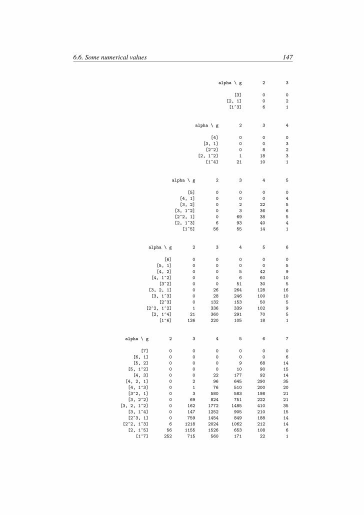
6.6. Some numerical values 147
alpha \ g 2 3
[3] 0 0
[2, 1] 0 2
[1^3] 6 1
alpha \ g 2 3 4
[4] 0 0 0
[3, 1] 0 0 3
[2^2] 0 8 2
[2, 1^2] 1 18 3
[1^4] 21 10 1
alpha \ g 2 3 4 5
[5] 0 0 0 0
[4, 1] 0 0 0 4
[3, 2] 0 2 22 5
[3, 1^2] 0 3 36 6
[2^2, 1] 0 69 38 5
[2, 1^3] 6 93 40 4
[1^5] 56 55 14 1
alpha \ g 2 3 4 5 6
[6] 0 0 0 0 0
[5, 1] 0 0 0 0 5
[4, 2] 0 0 5 42 9
[4, 1^2] 0 0 6 60 10
[3^2] 0 0 51 30 5
[3, 2, 1] 0 26 264 128 16
[3, 1^3] 0 28 246 100 10
[2^3] 0 132 153 50 5
[2^2, 1^2] 1 336 339 102 9
[2, 1^4] 21 360 291 70 5
[1^6] 126 220 105 18 1
alpha \ g 2 3 4 5 6 7
[7] 0 0 0 0 0 0
[6, 1] 0 0 0 0 0 6
[5, 2] 0 0 0 9 68 14
[5, 1^2] 0 0 0 10 90 15
[4, 3] 0 0 22 177 92 14
[4, 2, 1] 0 2 96 645 290 35
[4, 1^3] 0 1 76 510 200 20
[3^2, 1] 0 3 580 583 198 21
[3, 2^2] 0 69 824 751 222 21
[3, 2, 1^2] 0 162 1772 1485 410 35
[3, 1^4] 0 147 1252 905 210 15
[2^3, 1] 0 759 1454 849 188 14
[2^2, 1^3] 6 1218 2024 1062 212 14
[2, 1^5] 56 1155 1526 653 108 6
[1^7] 252 715 560 171 22 1
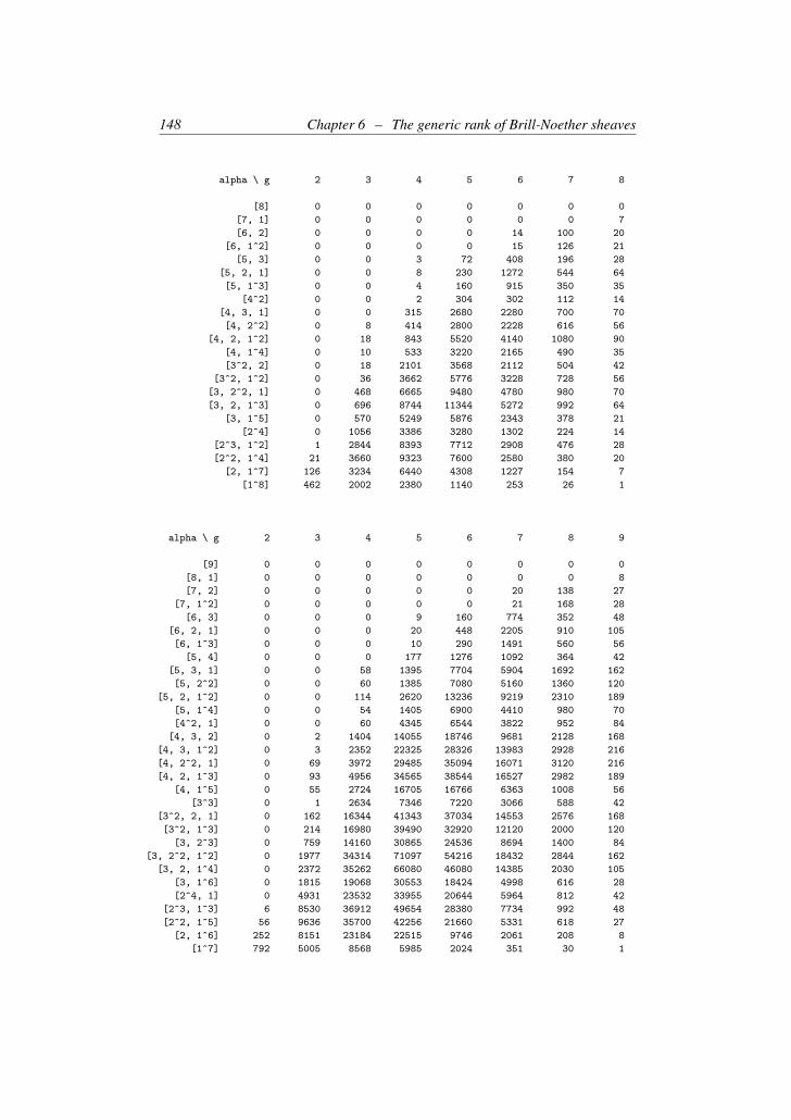
148 Chapter 6 – The generic rank of Brill-Noether sheaves
alpha \ g 2 3 4 5 6 7 8
[8] 0 0 0 0 0 0 0
[7, 1] 0 0 0 0 0 0 7
[6, 2] 0 0 0 0 14 100 20
[6, 1^2] 0 0 0 0 15 126 21
[5, 3] 0 0 3 72 408 196 28
[5, 2, 1] 0 0 8 230 1272 544 64
[5, 1^3] 0 0 4 160 915 350 35
[4^2] 0 0 2 304 302 112 14
[4, 3, 1] 0 0 315 2680 2280 700 70
[4, 2^2] 0 8 414 2800 2228 616 56
[4, 2, 1^2] 0 18 843 5520 4140 1080 90
[4, 1^4] 0 10 533 3220 2165 490 35
[3^2, 2] 0 18 2101 3568 2112 504 42
[3^2, 1^2] 0 36 3662 5776 3228 728 56
[3, 2^2, 1] 0 468 6665 9480 4780 980 70
[3, 2, 1^3] 0 696 8744 11344 5272 992 64
[3, 1^5] 0 570 5249 5876 2343 378 21
[2^4] 0 1056 3386 3280 1302 224 14
[2^3, 1^2] 1 2844 8393 7712 2908 476 28
[2^2, 1^4] 21 3660 9323 7600 2580 380 20
[2, 1^7] 126 3234 6440 4308 1227 154 7
[1^8] 462 2002 2380 1140 253 26 1
alpha \ g 2 3 4 5 6 7 8 9
[9] 0 0 0 0 0 0 0 0
[8, 1] 0 0 0 0 0 0 0 8
[7, 2] 0 0 0 0 0 20 138 27
[7, 1^2] 0 0 0 0 0 21 168 28
[6, 3] 0 0 0 9 160 774 352 48
[6, 2, 1] 0 0 0 20 448 2205 910 105
[6, 1^3] 0 0 0 10 290 1491 560 56
[5, 4] 0 0 0 177 1276 1092 364 42
[5, 3, 1] 0 0 58 1395 7704 5904 1692 162
[5, 2^2] 0 0 60 1385 7080 5160 1360 120
[5, 2, 1^2] 0 0 114 2620 13236 9219 2310 189
[5, 1^4] 0 0 54 1405 6900 4410 980 70
[4^2, 1] 0 0 60 4345 6544 3822 952 84
[4, 3, 2] 0 2 1404 14055 18746 9681 2128 168
[4, 3, 1^2] 0 3 2352 22325 28326 13983 2928 216
[4, 2^2, 1] 0 69 3972 29485 35094 16071 3120 216
[4, 2, 1^3] 0 93 4956 34565 38544 16527 2982 189
[4, 1^5] 0 55 2724 16705 16766 6363 1008 56
[3^3] 0 1 2634 7346 7220 3066 588 42
[3^2, 2, 1] 0 162 16344 41343 37034 14553 2576 168
[3^2, 1^3] 0 214 16980 39490 32920 12120 2000 120
[3, 2^3] 0 759 14160 30865 24536 8694 1400 84
[3, 2^2, 1^2] 0 1977 34314 71097 54216 18432 2844 162
[3, 2, 1^4] 0 2372 35262 66080 46080 14385 2030 105
[3, 1^6] 0 1815 19068 30553 18424 4998 616 28
[2^4, 1] 0 4931 23532 33955 20644 5964 812 42
[2^3, 1^3] 6 8530 36912 49654 28380 7734 992 48
[2^2, 1^5] 56 9636 35700 42256 21660 5331 618 27
[2, 1^6] 252 8151 23184 22515 9746 2061 208 8
[1^7] 792 5005 8568 5985 2024 351 30 1
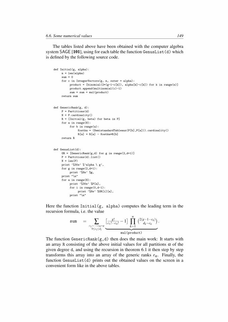
6.6. Some numerical values 149
The tables listed above have been obtained with the computer algebrasystem SAGE [101], using for each table the function GenusList(d) whichis defined by the following source code.
def Initial(g, alpha):
n = len(alpha)
sum = 0
for c in IntegerVectors(g, n, outer = alpha):
product = [binomial(2*(g-1-c[k]), alpha[k]-c[k]) for k in range(n)]
product.append(multinomial(c)-1)
sum = sum + mul(product)
return sum
def GenericRank(g, d):
P = Partitions(d)
N = P.cardinality()
R = [Initial(g, beta) for beta in P]
for a in range(N):
for b in range(a):
Kostka = (SemistandardTableaux(P[b],P[a])).cardinality()
R[a] = R[a] - Kostka*R[b]
return R
def GenusList(d):
GR = [GenericRank(g,d) for g in range(2,d+1)]
P = Partitions(d).list()
N = len(P)
print ’%30s’ %’alpha \ g’,
for g in range(2,d+1):
print ’%8s’ %g,
print "\n"
for a in range(N):
print ’%30s’ %P[a],
for i in range(0,d-1):
print ’%8s’ %GR[i][a],
print "\n"
Here the function Initial(g, alpha) computes the leading term in therecursion formula, i.e. the value
sum = ∑c1+···+cn=g
0≤ci≤di
[ g!c1!···cn! −1
] n
∏k=1
(2(g−1−ck)dk−ck
)︸ ︷︷ ︸
mul(product)
.
The function GenericRank(g,d) then does the main work: It starts withan array R consisting of the above initial values for all partitions α of thegiven degree d, and using the recursion in theorem 6.1 it then step by steptransforms this array into an array of the generic ranks rα . Finally, thefunction GenusList(d) prints out the obtained values on the screen in aconvenient form like in the above tables.

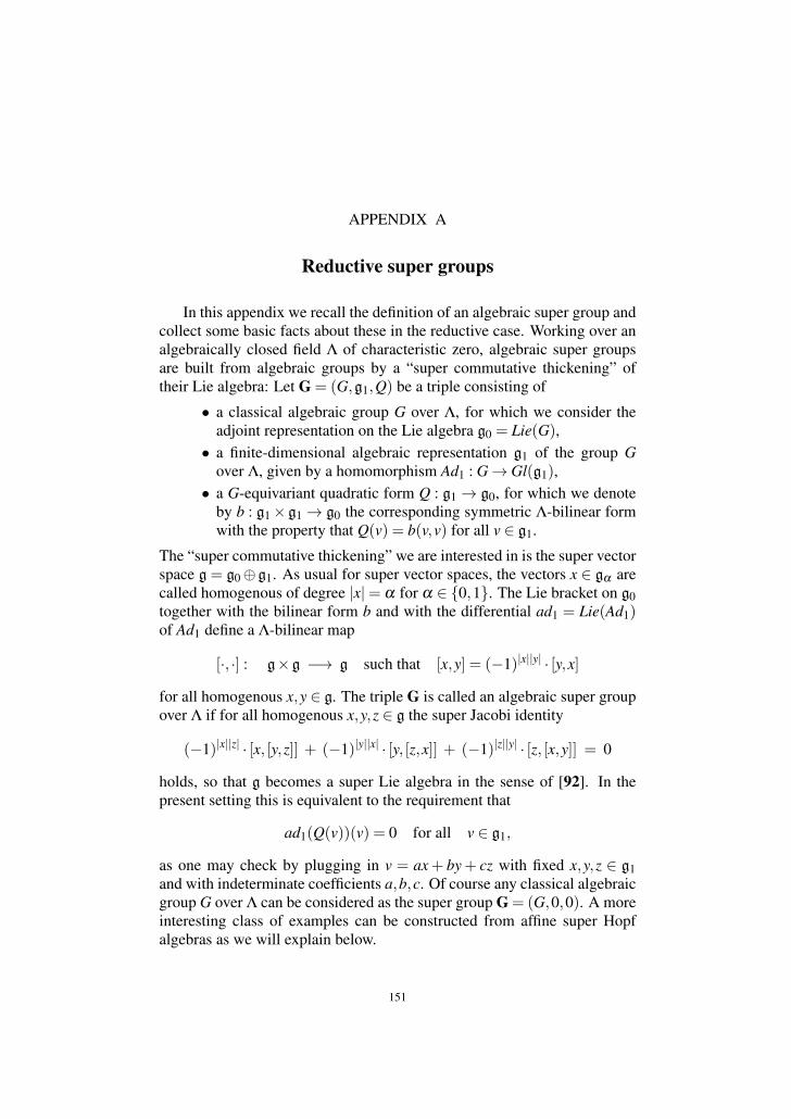
APPENDIX A
Reductive super groups
In this appendix we recall the definition of an algebraic super group andcollect some basic facts about these in the reductive case. Working over analgebraically closed field Λ of characteristic zero, algebraic super groupsare built from algebraic groups by a “super commutative thickening” oftheir Lie algebra: Let G = (G,g1,Q) be a triple consisting of
• a classical algebraic group G over Λ, for which we consider theadjoint representation on the Lie algebra g0 = Lie(G),• a finite-dimensional algebraic representation g1 of the group G
over Λ, given by a homomorphism Ad1 : G→ Gl(g1),• a G-equivariant quadratic form Q : g1→ g0, for which we denote
by b : g1×g1→ g0 the corresponding symmetric Λ-bilinear formwith the property that Q(v) = b(v,v) for all v ∈ g1.
The “super commutative thickening” we are interested in is the super vectorspace g= g0⊕g1. As usual for super vector spaces, the vectors x ∈ gα arecalled homogenous of degree |x|= α for α ∈ 0,1. The Lie bracket on g0together with the bilinear form b and with the differential ad1 = Lie(Ad1)of Ad1 define a Λ-bilinear map
[·, ·] : g×g −→ g such that [x,y] = (−1)|x||y| · [y,x]
for all homogenous x,y ∈ g. The triple G is called an algebraic super groupover Λ if for all homogenous x,y,z ∈ g the super Jacobi identity
(−1)|x||z| · [x, [y,z]] + (−1)|y||x| · [y, [z,x]] + (−1)|z||y| · [z, [x,y]] = 0
holds, so that g becomes a super Lie algebra in the sense of [92]. In thepresent setting this is equivalent to the requirement that
ad1(Q(v))(v) = 0 for all v ∈ g1,
as one may check by plugging in v = ax+ by+ cz with fixed x,y,z ∈ g1and with indeterminate coefficients a,b,c. Of course any classical algebraicgroup G over Λ can be considered as the super group G = (G,0,0). A moreinteresting class of examples can be constructed from affine super Hopfalgebras as we will explain below.
151
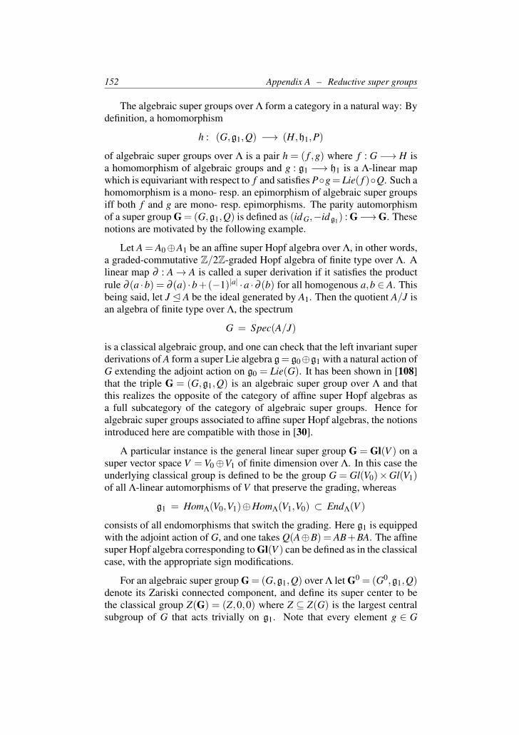
152 Appendix A – Reductive super groups
The algebraic super groups over Λ form a category in a natural way: Bydefinition, a homomorphism
h : (G,g1,Q) −→ (H,h1,P)
of algebraic super groups over Λ is a pair h = ( f ,g) where f : G −→ H isa homomorphism of algebraic groups and g : g1 −→ h1 is a Λ-linear mapwhich is equivariant with respect to f and satisfies Pg= Lie( f )Q. Such ahomomorphism is a mono- resp. an epimorphism of algebraic super groupsiff both f and g are mono- resp. epimorphisms. The parity automorphismof a super group G = (G,g1,Q) is defined as (id G,−idg1) : G−→G. Thesenotions are motivated by the following example.
Let A = A0⊕A1 be an affine super Hopf algebra over Λ, in other words,a graded-commutative Z/2Z-graded Hopf algebra of finite type over Λ. Alinear map ∂ : A→ A is called a super derivation if it satisfies the productrule ∂ (a ·b) = ∂ (a) ·b+(−1)|a| ·a ·∂ (b) for all homogenous a,b ∈ A. Thisbeing said, let J E A be the ideal generated by A1. Then the quotient A/J isan algebra of finite type over Λ, the spectrum
G = Spec(A/J)
is a classical algebraic group, and one can check that the left invariant superderivations of A form a super Lie algebra g= g0⊕g1 with a natural action ofG extending the adjoint action on g0 = Lie(G). It has been shown in [108]that the triple G = (G,g1,Q) is an algebraic super group over Λ and thatthis realizes the opposite of the category of affine super Hopf algebras asa full subcategory of the category of algebraic super groups. Hence foralgebraic super groups associated to affine super Hopf algebras, the notionsintroduced here are compatible with those in [30].
A particular instance is the general linear super group G = Gl(V ) on asuper vector space V =V0⊕V1 of finite dimension over Λ. In this case theunderlying classical group is defined to be the group G = Gl(V0)×Gl(V1)of all Λ-linear automorphisms of V that preserve the grading, whereas
g1 = HomΛ(V0,V1)⊕HomΛ(V1,V0) ⊂ EndΛ(V )
consists of all endomorphisms that switch the grading. Here g1 is equippedwith the adjoint action of G, and one takes Q(A⊕B) = AB+BA. The affinesuper Hopf algebra corresponding to Gl(V ) can be defined as in the classicalcase, with the appropriate sign modifications.
For an algebraic super group G = (G,g1,Q) over Λ let G0 = (G0,g1,Q)denote its Zariski connected component, and define its super center to bethe classical group Z(G) = (Z,0,0) where Z ⊆ Z(G) is the largest centralsubgroup of G that acts trivially on g1. Note that every element g ∈ G
153
induces an interior automorphism int(g) = (g−1 (−)g,Ad1(g)) of G andthat Z ⊆ G is the subgroup of all g ∈ G with int(g) = idG.
By a super representation of an algebraic super group G over Λ we meanan algebraic homomorphism ρV : G→Gl(V ) for a super vector space V offinite dimension over Λ. By definition, a homomorphism between superrepresentations ρV and ρW is a homomorphism V → W of super vectorspaces which preserves the gradings and intertwines ρV with ρW . One canshow that the category RepΛ(G) of all super representations of G over Λ isan abelian Λ-linear rigid symmetric monoidal category with respect to thesuper tensor product. We also have Schur’s lemma:
LEMMA A.1. For an irreducible super representation ρV : G→Gl(V ),every endomorphism of ρV has the form λ · idV with some scalar λ ∈ Λ.
Proof. The proof works as in the classical case. Note that by definitionwe only consider endomorphisms which preserve the grading; otherwiseSchur’s lemma would have to be modified, see [92, prop. 2, p. 46].
In particular, the super center Z(G) must act on any irreducible superrepresentation of G by a character χ : Z(G)→ Λ∗ (recall that Z(G) is aclassical commutative algebraic group and that each of its elements definesan endomorphism of any given super representation of G).
An algebraic super group G=(G,g1,Q) is called reductive if the abeliancategory RepΛ(G) is semisimple. The reductive algebraic super groupshave been classified in [108]. Every classical reductive algebraic groupG is also reductive when viewed as the super group G = (G,0,0). Anotherexample of reductive super groups is given by the orthosymplectic supergroups SpoΛ(2r,1) for r ∈ N which can be defined as follows: Let J be anon-degenerate antisymmetric 2r×2r matrix J = (Jik) over Λ. In terms ofthe classical symplectic group SpΛ(2r,J) = g ∈ GlΛ(2r) | gtJg = J wethen put
SpoΛ(2r,1) = (SpΛ(2r,J), Λ2r,Q),
where Λ2r is equipped with the standard action of SpΛ(2r,J) and where thequadratic map Q : Λ2r→ Lie(SpΛ(2r,J)) is defined by Q(v)ik = ∑
2rl=1 vivlJlk
in the standard coordinates. In particular, we have a natural representationof the super group SpoΛ(2r,1) on the super vector space V = V0⊕V1 witheven part V0 = Λ2r and odd part V1 = Λ. On the odd part of the super Liealgebra this representation is given by
Λ2r 3 v 7→
((1 7→ v)⊕ (w 7→ wtJv)
)∈ HomΛ(V1,V0)⊕HomΛ(V0,V1).
Of course a different choice of the non-degenerate antisymmetric matrix Jwill result in an isomorphic super group SpoΛ(2r,1).
154 Appendix A – Reductive super groups
It turns out that the above examples essentially exhaust all reductivealgebraic super groups over Λ. Indeed, by theorem 6 of loc. cit. an algebraicsuper group G over Λ is reductive iff there are a classical reductive group Hand integers N ∈ N0, ni,ri ∈ N such that G is isomorphic to a semidirectproduct
G =( N
∏i=1
(SpoΛ(2ri,1)
)ni)oH
with respect to a homomorphism π0(H)→∏Ni=1Sni where each symmetric
group Sni acts on(SpoΛ(2ri,1)
)ni by permutation of the factors.
COROLLARY A.2. For a reductive algebraic super group G over Λ, theunderlying classical group G is reductive as well; furthermore, the supercenter Z(G) is a subgroup of finite index in the classical center Z(G).
Proof. By the above it suffices to show this in case G = SpoΛ(2r,1) forsome r ∈ N. But then G = SpΛ(2r), and Z(G) = µ2 is finite.
PROPOSITION A.3. Let h : G1→ G0 be a homomorphism of reductivesuper groups over Λ which induces an epimorphism
f : G1 G0
on the underlying classical groups. If the super center Z(G0) contains aclassical torus T0, then also Z(G1) contains a classical torus T1 such thatthe epimorphism f restricts to an isogeny p : T1→ T0.
Proof. The category of tori (or diagonalizable groups) over Λ, up toisogeny, is equivalent to the category of finite vector spaces over Q via thecocharacter functor T 7→ X(T ) = Hom(Gm,T )⊗ZQ. If π is a finite groupacting on T , then we have
X((T π)0) = (X(T ))π
for the invariants of the action on the torus resp. on its cocharacters.
For reductive super groups G we have Z(G)0 = Z(G)0 by corollary A.2.On Z(G0) the group G acts by conjugation, and this action factors over thefinite group π = π0(G). By definition we have Z(G)0 ⊂ Z(G0)π , and this isa subgroup of finite index: This follows by an application of the cocharacterfunctor since X(Z(G)0) = X(Z(G0))π .
For the proof of the proposition it suffices to show that T0 is containedin the image of Z(G1)
0. By assumption h induces an epimorphism of theunderlying classical groups, hence an epimorphism f : (G1)
0 → (G0)0 of
their connected components. By the theory of connected reductive classical
155
groups, the torus T = Z((G0)0)0 is the image of S = Z((G1)
0)0. Now frestricts to a homomorphism
f : S −→ T
and this homomorphism is equivariant for the action of π = π0(G1) on Sand T , where by the action on T we mean the one induced by the naturalhomomorphism π0(G1) → π0(G0). We claim that f : (Sπ)0 → (T π)0 issurjective: Indeed, the functor of invariants under a finite group π is rightexact on finite-dimensional vector spaces over Q. Since (Sπ)0 ⊂ Z(G1)
0
and T0 ⊂ (T π)0 this completes the proof.

APPENDIX B
Irreducible subgroups with bounded determinant
In this appendix we discuss the facts from representation theory thathave been used to obtain the finiteness result in lemma 3.19. The basis forthis is the following extended version of the fundamental result of [109],where by P(X) = Perv(X ,C) we denote as before the category of perversesheaves on a complex abelian variety X .
LEMMA B.1. Let P ∈ P(X) be a semisimple perverse sheaf, G = G(P)the associated Tannaka group and H = G0 its connected component. Thenthe group π = G/H of connected components is a finite abelian groupwhose conjugation action is trivial on the torus Hab = H/[H,H].
Proof. By loc. cit. the group π = G/H of connected components is afinite abelian group, and its characters correspond to skyscraper sheaves δxsupported on torsion points x∈X . Thus the group Hom(π,C∗) of characterscan be identified in a natural way with a finite subgroup K ⊆ X of torsionpoints. Consider then the etale isogeny
f : X −→ Y = X/K.
Since |K|= [G : H], lemma 1 in loc. cit. shows that the component H = G0
coincides with the Tannaka group H = G( f∗(P)) of the direct image andthat the adjoint functors
P(X)
f∗))P(Y )
f ∗ii
correspond to RepC(G)
ResGH++RepC(H).
IndGH
kk
Now put m = |K|. For any closed point y∈Y the pull-back f ∗(δy) is a directsum of rank one skyscraper sheaves supported on the m distinct point of thefibre f−1(y), hence f∗( f ∗(δy)) = (δy)
⊕m is an isotypic multiple of δy. Inother words
ResGH(IndG
H(χ)) is isotypic for all χ ∈ Hom(H,C∗).Going back to the construction of induced representations, it follows thatevery character χ : H −→ C∗ is invariant under conjugation by G. Via theequivalence between connected tori and their character groups this impliesthat G/H acts trivially on the torus Hab = H/[H,H].
157
158 Appendix B – Irreducible subgroups with bounded determinant
With this input from geometry, the rest of the argument for the desiredfiniteness result will be an exercise in representation theory. Recall that acomplex algebraic group G is reductive iff the abelian category RepC(G)of its finite-dimensional representations over C is semisimple, which is thecase iff G admits a faithful irreducible representation. This is in particularthe case for any irreducible subgroup G →Gl(V ) of the general linear groupattached to a finite-dimensional complex vector space V , where as usual byan irreducible subgroup we mean a subgroup which acts irreducibly on thegiven vector space. The result we are looking for is the following.
LEMMA B.2. Fix an integer n ∈ N, and let V be a finite-dimensionalcomplex vector space. Then up to conjugacy there exist only finitely manyirreducible algebraic subgroups G → Gl(V ) such that
(a) the quotient π = G/H by the connected component H = G0 is afinite abelian group, and
(b) via conjugation π acts trivially on Hab = H/[H,H], and(c) the determinant det(V ) is a character of G of order at most n.
Proof. Using the structure theory of connected reductive groups andthe fact that every such group has at most finitely many representationsof any given dimension, one checks that up to conjugation there are onlyfinitely many connected reductive algebraic subgroups H → Gl(V ). So itwill be enough to show that for any given H there exist only finitely manyirreducible subgroups G →Gl(V ) with connected component G0 = H suchthat (a) – (c) hold. For this we will show that every such subgroup G canbe recovered from the connected component G0 = H together with certainfinite data. We proceed in the following steps.
Step 1. Let G∗⊆G be a normal subgroup of finite index, and decomposethe restriction of the given representation as V |G∗ =
⊕mi=1Vi with irreducible
representations Vi ∈ RepC(G∗). Then we claim that for each index i the
determinant character
det(Vi) : G∗ −→ C∗
is a character of order at most m · n. Indeed, by the bound in (c) it will beenough to show that det(Vi) does not depend on i. Note that each g ∈ Gdefines an automorphism int(g) : G∗ −→ G∗, and since V is an irreduciblerepresentation of G, all the irreducible constituents Vi of the restriction V |G∗are conjugate to each other by such inner automorphisms. Hence it followsfrom assumption (b) that the restriction det(Vi)|H does not depend on theindex i. Again by the bound in (c) this restriction is then a torsion characterof the connected group Hab and as such it must be trivial. Thus all thedet(Vi) are characters of the quotient group G∗/H. By assumption (a) theadjoint action of G on this quotient group is trivial, so our claim follows.
159
Step 2. We now apply step 1 as follows. Let U ⊆V |H be an irreducibleconstituent of the restriction of V to the connected component G0 = H, andconsider the stabilizer
G∗ =
g ∈ G | gU ∼= U in RepC(H)⊆ G.
We define the isotypic part W ⊆V |H to be the sum of all subrepresentationsof V |H which are isomorphic to the chosen representation U . Then W is arepresentation of G∗, and a version of Mackey’s lemma shows that
V ∼= IndGG∗(W )
is isomorphic to the representation induced from W . Since V ∈ RepC(G)is irreducible, it follows that W ∈ RepC(G
∗) is irreducible as well. Butthe group π∗ = G∗/H of connected components is abelian by (a) and therestriction W |H is isotypic, hence lemma B.3 below shows that even W |His irreducible. Hence in step 1 we can take V1 = W , and accordingly eachof the conjugate representations V1, . . . ,Vm is stable under the group G∗ andirreducible. For the centralizer of the subgroup H in G then
ZG(H) → ZG∗(H) →m
∏i=1
C∗ · idVi,
where the first inclusion comes from the fact that the centralizer preserveseach isotypic component and is therefore contained in G∗ and where thesecond inclusion comes from Schur’s lemma. So each element of ZG(H)acts on each Vi by a scalar, and by step 1 this scalar is a root of unity ofbounded order. Hence ZG(H) is a finite group of bounded order.
Step 3. This being said, let us fix as before a connected and reductivesubgroup H → Gl(V ). By [99, cor. 2.14] the short exact sequence of innerand outer automorphism groups admits a splitting
1 // Int(H) // Aut(H) // Out(H) //
∃sxx
1
with some section s. In what follows we will fix such a section once andfor all. If G → Gl(V ) is an irreducible algebraic subgroup with G0 = Hand such that (a) – (c) hold, we want to show that G can be recoveredfrom certain finite data involving H and s. To achieve this, consider theconjugation action
int : G −→ Aut(H)
and denote by F = int−1(Im(s)) ⊂ G the preimage of the section s. Byconstruction we have an exact sequence
1 // ZG(H) // Fϕ// Out(H)
160 Appendix B – Irreducible subgroups with bounded determinant
where ZG(H) = ker(ϕ) denotes the centralizer of H in G. By Step 2 thiscentralizer and hence also F is finite of bounded order. Furthermore, fromthe definitions one checks that the homomorphism
π : H oϕ F −→ G, (h, f ) 7→ h f
is an epimorphism and that ker(π) ⊆ Z(H)oϕ F where Z(H) denotes thecenter of H. Note that by Schur’s lemma this center acts by a scalar on eachisotypic component of V |H , in particular Z(H) is a finite group of boundedorder in view of the bound for the determinant in step 1.
Thus any irreducible algebraic subgroup G → Gl(V ) with G0 = H andwith properties (a) – (c) is isomorphic to a quotient
G ∼= (H oϕ F)/K
where F is a finite group of bounded order, acting on the group H via ahomomorphism ϕ : F → Aut(H) with image in the finite group s(Out(H)),and where K is a subgroup of the finite group Z(H)oϕ F . Hence for theisomorphism type of G there are only finitely many possibilities.
Finally, for (F,ϕ,K) as above, any embedding (H oϕ F)/K → Gl(V )which extends the given embedding of H is determined uniquely by thehomomorphism ρ : F −→ Gl(V ) it induces. We claim that under the givenconditions there exist only finitely many such ρ . Indeed, if ρ is any othersuch homomorphism, then for any f ∈ F one computes that
ρ( f ) · ρ( f )−1 ∈ ZGl(V )(H) =m
∏i=1
C∗ · idVi
where the last equality holds by Schur’s lemma, and in view of the boundon the determinant in step 1 the centralizer ZGl(V )(H) is finite.
In step 2 of the above proof we have used the following fact, where wereset our notations and replace G∗ by G for simplicity.
LEMMA B.3. Let W be a finite-dimensional complex vector space, Gan irreducible subgroup of Gl(W ) whose group G/G0 of components isabelian, and H →G a subgroup of finite index such that the restriction W |His isotypic. Then in fact W |H is irreducible.
Proof. By devissage for the finite abelian group G/H it will be enoughto show this when G/H ∼= Z/mZ is a finite cyclic group. Furthermore, bythe assumption of being isotypic we can write
W |H = U⊗Cn
for some irreducible representation U ∈ RepC(H) and some n ∈ N. Wemust show n = 1. Since G/G0 is abelian, the finite index subgroup H ⊆ G
161
is automatically a normal subgroup. Hence
G → NGl(W )(H) = NGl(U)(H)⊗Gln(C)where the last equality follows via a block matrix calculation from Schur’slemma; here the tensor product on the right hand side denotes the image ofthe natural homomorphism f : NGl(U)(H)×Gln(C) −→ Gl(U ⊗Cn). Nowlet G = f−1(G). If 1 denotes the trivial subgroup of Gln(C), then we havean epimorphism
G/(H×1) G/Hwith central kernel (this follows from the fact that f has central kernel). Butby assumption the group G/H is cyclic, and any central extension of a cyclicgroup is an abelian group — being generated by a central subgroup togetherwith a single further element. Hence G/(H × 1) is an abelian group. Onthe other hand this abelian group must act irreducibly on Cn because G actsirreducibly on W . So it follows that n = 1.
We conclude this appendix with the following result which does notdirectly depend on the above but also involves a Mackey-type argumentand has been used in lemma 4.13 to control the possible non-connectednessof the Tannaka group attached to the theta divisor.
LEMMA B.4. Let G be a complex reductive group whose group G/G0
of connected components is abelian, and let V ∈ RepC(G) be an irreduciblerepresentation. If the restriction V |G0 is reducible, then for some non-trivialcharacter χ : G−→ C∗ there exists an isomorphism V ∼=V ⊗C χ .
Proof. Consider the tensor product W = V ⊗C V∨ ∈ RepC(G) of thegiven representation with its dual. We must show that this tensor productcontains a non-trivial one-dimensional representation χ : G −→ C∗ as adirect summand. Note that since H = G0 is a normal subgroup of G, thespace of H-invariants
W H = w ∈W | hw = w ∀h ∈ H ⊂ W
is stable under the action of G and hence defines a representation of the finiteabelian group G/H. As such it splits into a direct sum of one-dimensionalrepresentations. Among these the trivial representation 1 occurs preciselyonce because by adjunction dimC(HomG(1,W )) = dimC(HomG(V,V )) = 1,using that V is an irreducible representation of G so that Schur’s lemmaapplies. So it will be enough to show that
dimC(W H) > 1 if V |H is reducible.
But this follows from the observation that if the restriction U = V |H splitsinto n direct summands, then W |H =U ⊗CU∨ contains at least n copies ofthe one-dimensional trivial representation.

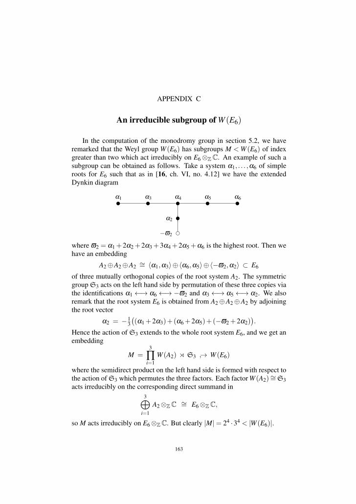
APPENDIX C
An irreducible subgroup of W (E6)
In the computation of the monodromy group in section 5.2, we haveremarked that the Weyl group W (E6) has subgroups M < W (E6) of indexgreater than two which act irreducibly on E6⊗ZC. An example of such asubgroup can be obtained as follows. Take a system α1, . . . ,α6 of simpleroots for E6 such that as in [16, ch. VI, no. 4.12] we have the extendedDynkin diagram
u u u u uue
α1 α3 α4 α5 α6
α2
−ϖ2
where ϖ2 = α1 +2α2 +2α3 +3α4 +2α5 +α6 is the highest root. Then wehave an embedding
A2⊕A2⊕A2 ∼= 〈α1,α3〉⊕〈α6,α5〉⊕〈−ϖ2,α2〉 ⊂ E6
of three mutually orthogonal copies of the root system A2. The symmetricgroup S3 acts on the left hand side by permutation of these three copies viathe identifications α1←→ α6←→−ϖ2 and α3←→ α5←→ α2. We alsoremark that the root system E6 is obtained from A2⊕A2⊕A2 by adjoiningthe root vector
α2 = −13
((α1 +2α3)+(α6 +2α5)+(−ϖ2 +2α2)
).
Hence the action of S3 extends to the whole root system E6, and we get anembedding
M =3
∏i=1
W (A2) o S3 → W (E6)
where the semidirect product on the left hand side is formed with respect tothe action of S3 which permutes the three factors. Each factor W (A2)∼=S3acts irreducibly on the corresponding direct summand in
3⊕i=1
A2⊗ZC ∼= E6⊗ZC,
so M acts irreducibly on E6⊗ZC. But clearly |M|= 24 ·34 < |W (E6)|.
163

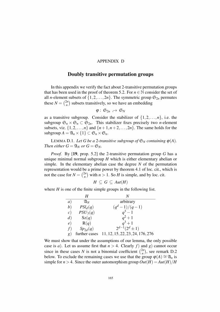
APPENDIX D
Doubly transitive permutation groups
In this appendix we verify the fact about 2-transitive permutation groupsthat has been used in the proof of theorem 5.2. For n∈N consider the set ofall n-element subsets of 1,2, . . . ,2n. The symmetric group S2n permutesthese N =
(2nn
)subsets transitively, so we have an embedding
ϕ : S2n → SN
as a transitive subgroup. Consider the stabilizer of 1,2, . . . ,n, i.e. thesubgroup Sn×Sn ⊂ S2n. This stabilizer fixes precisely two n-elementsubsets, viz. 1,2, . . . ,n and n+1,n+2, . . . ,2n. The same holds for thesubgroup A = An×1 ⊂Sn×Sn.
LEMMA D.1. Let G be a 2-transitive subgroup of SN containing ϕ(A).Then either G = AN or G =SN .
Proof. By [19, prop. 5.2] the 2-transitive permutation group G has aunique minimal normal subgroup H which is either elementary abelian orsimple. In the elementary abelian case the degree N of the permutationrepresentation would be a prime power by theorem 4.1 of loc. cit., which isnot the case for N =
(2nn
)with n > 1. So H is simple, and by loc. cit.
H ⊆ G ⊆ Aut(H)
where H is one of the finite simple groups in the following list.
H Na) AN arbitraryb) PSld(q) (qd−1)/(q−1)c) PSU3(q) q3−1d) Sz(q) q2 +1e) R(q) q3 +1f ) Sp2d(q) 2d−1(2d±1)g) further cases 11,12,15,22,23,24,176,276
We must show that under the assumptions of our lemma, the only possiblecase is a). Let us assume first that n > 4. Clearly f ) and g) cannot occursince in these cases N is not a binomial coefficient
(2nn
), see remark D.2
below. To exclude the remaining cases we use that the group ϕ(A)∼= An issimple for n> 4. Since the outer automorphism group Out(H) =Aut(H)/H
165
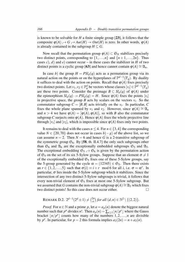
166 Appendix D – Doubly transitive permutation groups
is known to be solvable for H a finite simple group [23], it follows that thecomposite ϕ(A) → G → Aut(H) Out(H) is zero. In other words, ϕ(A)is already contained in the subgroup H ⊆ G.
Now recall that the permutation group ϕ(A) ⊂SN stabilizes preciselytwo distinct points, corresponding to 1, . . . ,n and n+ 1, . . . ,2n. Thuscases c), d) and e) cannot occur – in these cases the stabilizer in H of twodistinct points is a cyclic group [63] and hence cannot contain ϕ(A)∼= An.
In case b) the group H = PSld(q) acts as a permutation group via itsnatural action on the points or on the hyperplanes of Pd−1(Fq). By dualityit suffices to deal with the action on points. Recall that ϕ(A) fixes preciselytwo distinct points. Let v1,v2 ∈ Fd
q be vectors whose classes [vi]∈ Pd−1(Fq)are these two points. Consider the preimage B ⊂ Sld(q) of ϕ(A) underthe epimorphism Sld(q) PSld(q) = H. Since ϕ(A) fixes the points [vi]in projective space, the group B acts by scalars on the vectors vi. So thecommutator subgroup C = [B,B] acts trivially on the vi. In particular, Cfixes the whole plane spanned by v1 and v2. However, since ϕ(A) ∼= Anand n > 4 we have ϕ(A) = [ϕ(A),ϕ(A)], so with B also the commutatorsubgroup C surjects onto ϕ(A). Hence ϕ(A) fixes the whole projective linethrough [v1] and [v2], which is impossible since ϕ(A) fixes only two points.
It remains to deal with the cases n≤ 4. For n∈ 3,4 the correspondingvalue N ∈ 20,70 does not occur in cases b) - g) of the above list, so wecan assume n = 2. Then N = 6 and hence G is a 2-transitive subgroup ofthe symmetric group S6. By [58, th. II.4.7] the only such subgroups otherthan S6 and A6 are the exceptionally embedded subgroups S5 and A5.The exceptional embedding S5 → S6 is given by the permutation actionof S5 on the set of its six 5-Sylow groups. Suppose that an element σ 6= 1of the exceptionally embedded S5 fixes one of these 5-Sylow groups, saythe 5-group generated by the cycle α = (12345) ∈ S5. Then there existsan r ∈ 1,2, . . . ,5 such that σ(i) ≡ i+ r mod 6 for all i, i.e. σ = αr. Inparticular, σ lies inside the 5-Sylow subgroup which it stabilizes. Since theintersection of any two distinct 5-Sylow subgroups is trivial, it follows thatevery non-trivial element of S5 fixes at most one 5-Sylow subgroup. Butwe assumed that G contains the non-trivial subgroup ϕ(A)∼=A2 which fixestwo distinct points! So this case does not occur either.
REMARK D.2. 2d−1(2d±1) 6=(2n
n
)for all (d,n) ∈ N2 \(2,2).
Proof. For n ∈N and a prime p, let a = ap(n) denote the biggest naturalnumber such that pa divides n!. Then ap(n) = ∑e≥1bn/pecwhere the Gaussbracket bn/pec counts how many of the numbers 1,2, . . . ,n are divisibleby pe. In particular, for p = 2 this formula implies a2(2n) = n+a2(n).
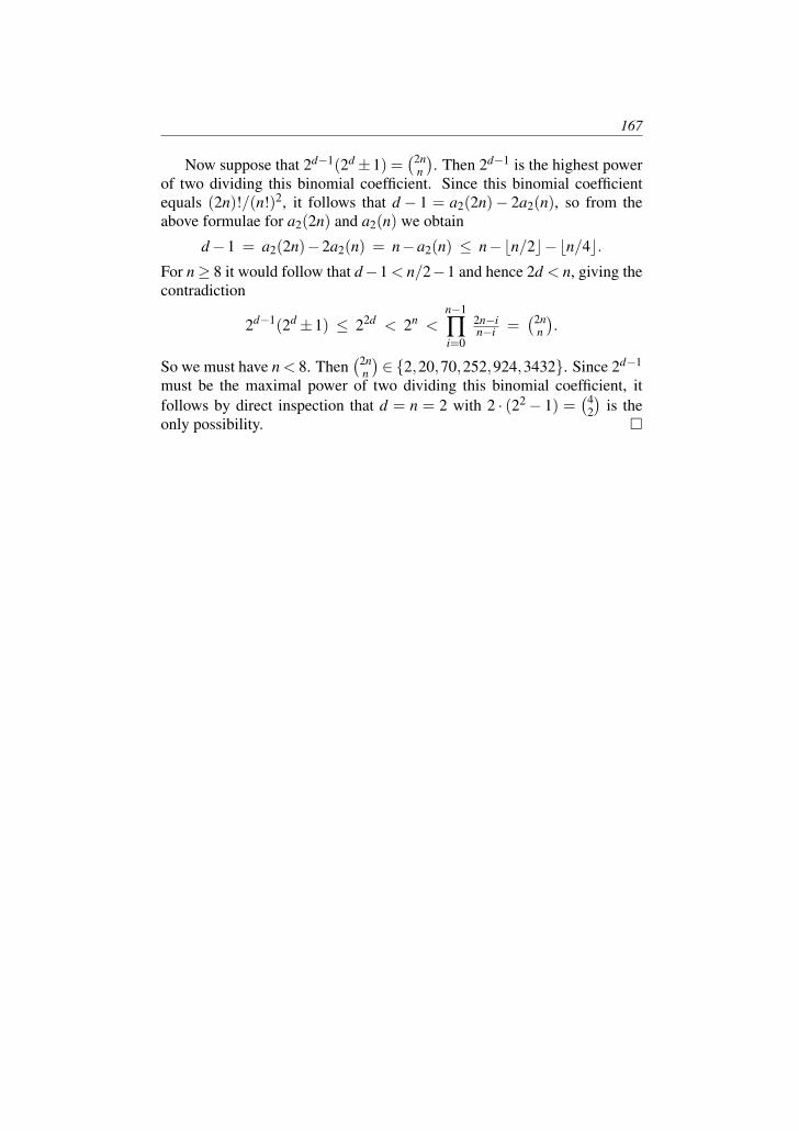
167
Now suppose that 2d−1(2d±1) =(2n
n
). Then 2d−1 is the highest power
of two dividing this binomial coefficient. Since this binomial coefficientequals (2n)!/(n!)2, it follows that d − 1 = a2(2n)− 2a2(n), so from theabove formulae for a2(2n) and a2(n) we obtain
d−1 = a2(2n)−2a2(n) = n−a2(n) ≤ n−bn/2c−bn/4c.For n≥ 8 it would follow that d−1 < n/2−1 and hence 2d < n, giving thecontradiction
2d−1(2d±1) ≤ 22d < 2n <n−1
∏i=0
2n−in−i =
(2nn
).
So we must have n < 8. Then(2n
n
)∈ 2,20,70,252,924,3432. Since 2d−1
must be the maximal power of two dividing this binomial coefficient, itfollows by direct inspection that d = n = 2 with 2 · (22− 1) =
(42
)is the
only possibility.

Bibliography
1. Andre, Y. and Kahn, B., Nilpotence, radicaux et structures monoidales, Rend. Sem.Mat. Univ. Padova 108 (2002), 107–209.
2. , Erratum: Nilpotence, radicaux et structures monoidales, Rend. Sem. Mat.Univ. Padova 113 (2005), 125–128.
3. Andreev, E. M., Vinberg, E. B. and Elashvili, A. G., Orbits of greatest dimension insemi-simple linear Lie groups, Funct. Anal. Appl. 1 (1967), 257–261.
4. Andreotti, A. and Mayer, A. L., On period relations for abelian integrals on algebraiccurves, Ann. Sc. Norm. Super. Pisa Cl. Sci. 21 (1967), 189–238.
5. Arbarello, E., Cornalba, M. and Griffiths, P. A., Geometry of algebraic curves II,Grundlehren Math. Wiss., vol. 268, Springer Verlag, 2011.
6. Arbarello, E., Cornalba, M., Griffiths, P. A. and Harris, J., Geometry of algebraiccurves, Grundlehren Math. Wiss., vol. 267, Springer Verlag, 1985.
7. Artin, M., Grothendieck, A. and Verdier, J.-L. (eds.), Seminaire de geometriealgebrique du Bois Marie 1963-64. Theorie des topos et cohomologie etale desschemas (SGA 4), Lecture Notes in Math., vol. 269, 270, 305, Springer Verlag, 1972.
8. Beauville, A., Prym varieties and the Schottky problem, Invent. Math. 41 (1977),149–196.
9. Beilinson, A. and Bernstein, J., A proof of Jantzen conjectures, Adv. Soviet Math. 16(1993), 1–50.
10. Beilinson, A., Bernstein, J. and Deligne, P., Faisceaux Pervers, Asterisque 100(1982).
11. Bierstone, E. and Milman, D., Canonical desingularization in characteristic zeroby blowing up the maximum strata of a local invariant, Invent. Math. 128 (1997),207–302.
12. Bingener, J. and Flenner, H., Constructible and quasiconstructible sheaves, Abh.Math. Sem. Univ. Hamburg 54 (1984), 119–139.
13. Birkenhake, C. and Lange, H., Complex abelian varieties (second ed.), GrundlehrenMath. Wiss., vol. 302, Springer Verlag, 2004.
14. Bockle, G. and Khare, C., Mod l representations of arithmetic fundamental groups.II. A conjecture of A. J. de Jong, Compos. Math. 142 (2006), 271–294.
15. Bosch, S., Lutkebohmert, W. and Raynaud, M., Neron models, Ergeb. Math. Grenz-geb. (3. Folge), vol. 21, Springer Verlag, 1990.
16. Bourbaki, N., Groupes et algebres de Lie. Chapitres 4, 5 et 6, Herrmann, 1968.17. Brion, M. and Szamuely, T., Prime-to-p etale covers of algebraic groups and ho-
mogenous spaces, arxiv:1109.2802v3.18. Brown, K. S., Cohomology of groups, Grad. Texts in Math., vol. 87, Springer Verlag,
1982.19. Cameron, P. J., Finite permutation groups and finite simple groups, Bull. London
Math. Soc. 13 (1980), 1–22.
169
170 Bibliography
20. Ciliberto, C. and van der Geer, G., Andreotti-Mayer loci and the Schottky problem,Doc. Math. 13 (2008), 453–504.
21. Conway, J. H. and Sloane, N. J. A., Low-dimensional lattices. I. Quadratic forms ofsmall determinant, Proc. R. Soc. Lond. A 418 (1988), 17–41.
22. , Sphere packings, lattices and groups (third ed.), Grundlehren Math. Wiss.,vol. 290, Springer Verlag, 199.
23. Conway, J. H. et al., ATLAS of finite groups, Clarendon Press, 1985.24. O. Debarre and E. Izadi, Ampleness of intersections of translates of theta divisors in
an abelian fourfold, Proc. Amer. Math. Soc. 135 (2007), 3477–3483.25. Debarre, O., Sur la demonstration de A. Weil du theoreme de Torelli pour les courbes,
Compos. Math. 58 (1986), 3–11.26. , Le lieu des varietes abeliennes dont le diviseur theta est singulier a deux
composantes, Ann. Sci. Ec. Norm. Super. 25 (1992), 687–708.27. , The Schottky problem – an update, Complex algebraic geometry, Math. Sci.
Res. Inst. Publ., vol. 28, 1995, pp. 57–64.28. Deligne, P., La conjecture de Weil II, Publ. Math. Inst. Hautes Etudes Sci. 52 (1980),
137–252.29. , Hodge cycles on abelian varieties, Hodge cycles, Motives and Shimura
varieties, Lecture Notes in Math., vol. 900, Springer Verlag, 1982, pp. 9–100.30. , Categories tensorielles, Moscow Math. J. 2 (2002), 227–248.31. , Categories Tannakiennes, The Grothendieck Festschrift, vol. II, Modern
Birkhauser Classics, 2007, pp. 111–195.32. Deligne, P. and Katz, N. (eds.), Seminaire de geometrie algebrique du Bois Marie
1967-1969. Groupes de monodromie en geometrie algebrique (SGA7), Lecture Notesin Math., vol. 288 and 340, Springer Verlag, 1972-73.
33. Deligne, P. and Milne, J. S., Tannakian categories, Hodge Cycles, Motives,and Shimura varieties, Lecture Notes in Math., vol. 900, Springer Verlag, 1982,pp. 101–228.
34. Donagi, R., The fibers of the Prym map, Contemporary Mathematics 136 (1992),55–125.
35. Drinfeld, V., On a conjecture of Kashiwara, Math. Res. Lett. 8 (2001), 713–728.36. Ein, L. and Lazarsfeld, R., Singularities of theta divisors and the birational geometry
of irregular varieties, Journal of the AMS 10, 243–258.37. Franecki, J. and Kapranov, M., The Gauss map and a noncompact Riemann-Roch
formula for constructible sheaves on semiabelian varieties, Duke Math. J. 104(2000), 171–180.
38. Freitag, E. and Kiehl, R., Etale cohomology and the Weil conjecture, Springer Verlag,1988.
39. Friedman, R. and Smith, R., The generic Torelli theorem for the Prym map, Invent.Math. 67 (1982), 473–490.
40. Fulton, W., Intersection theory (second ed.), Springer Verlag, 1998.41. Gabber, O. and Loeser, F., Faisceaux pervers `-adiques sur un tore, Duke Math. J.
83 (1996), 501–606.42. Gabriel, P., Des categories abeliennes, Bull. Soc. Math. France 90 (1962), 323–448.43. Gaitsgory, D., On de Jong’s conjecture, Israel J. Math. 157 (2007), 155–191.44. Ginzburg, V., Characteristic varieties and vanishing cycles, Invent. Math. 84 (1986),
327–402.45. Gompf, R. E. and Stipsicz, A. I., 4-manifolds and Kirby calculus, Grad. Stud. Math.,
Amer. Math. Soc., 1999.
171
46. Goodman, R. and Wallach, N. R., Symmetry, representations and invariants, SpringerVerlag, 2009.
47. Green, M. and Lazarsfeld, R., Deformation theory, generic vanishing theorems,and some conjectures of enriques, catanese and beauville, Invent. Math. 90 (1987),389–407.
48. Griffiths, P. and Harris, J., Principles of algebraic geometry, Wiley & Sons, 1978.49. Grothendieck, A., Elements de geometrie algebrique (rediges avec la collaboration
de Jean Dieudonne): IV. Etude locale des schemas et des morphismes de schemas.Seconde partie, Publ. Math. Inst. Hautes Etudes Sci. 24 (1965), 5–231.
50. , Elements de geometrie algebrique (rediges avec la collaboration de JeanDieudonne): IV. Etude locale des schemas et des morphismes de schemas. Troisiemepartie, Publ. Math. Inst. Hautes Etudes Sci. 28 (1966), 5–255.
51. , Seminaire de geometrie algebrique du Bois Marie 1960-61. Revetementsetales et groupe fondamental (SGA 1), Lecture Notes in Math., vol. 224, SpringerVerlag, 1971.
52. Grothendieck, A. and Murre, J. P., The tame fundamental group of a formal neigh-bourhood of a divisor with normal crossings on a scheme, Lecture Notes in Math.,vol. 208, Springer Verlag, 1971.
53. Grushevsky, S. and Salvati Manni, R., Singularities of the theta divisor at points oforder two, Int. Math. Res. Not. IMRN (2007), doi:10.1093/imrn/rnm045.
54. , Jacobians with a vanishing theta-null in genus 4, Israel J. Math. 164 (2008),303–315.
55. Hartshorne, R., Algebraic geometry, Grad. Texts in Math., vol. 52, Springer Verlag,1977.
56. Hironaka, H., Introduction to the theory of infinitesimally near singular points, Mem.Math. Inst. Jorge Juan 28 (1974).
57. Hotta, R., Takeuchi, K. and Tanisaki, T., D-modules, perverse sheaves and represen-tation theory, Progress in Math., vol. 236, Birkhauser, 2008.
58. Huppert, B., Endliche Gruppen I, Grundlehren Math. Wiss., vol. 134, Springer Ver-lag, 1976.
59. Illusie, L., Theorie de Brauer et caracteristique d’Euler-Poincare, Asterisque 82-83(1981), 161–172.
60. , Autour du theoreme de monodromie locale, Asterisque 223 (1994), 9–57.61. Izadi, E., The geometric structure of A4, the structure of the Prym map, double solids
and Γ00-divisors, J. Reine Angew. Math. 462 (1995), 93–158.62. James, D. G., On Witt’s theorem for unimodular quadratic forms, Pacific J. Math. 26
(1968), 303–316.63. Kantor, W. M., O’Nan, M. E. and Seitz, G. M., 2-transitive groups in which the
stabilizer of two points is cyclic, J. Alg. 21 (1972), 17–50.64. Katz, N. M. and Laumon, G., Transformation de Fourier et majoration de sommes
exponentielles, Publ. Math. Inst. Hautes Etudes Sci. 62 (1985), 145–202.65. Kiehl, E. and Weissauer, R., Weil conjectures, perverse sheaves and l-adic Fourier
transform, Ergeb. Math. Grenzgeb. (3. Folge), vol. 42, Springer Verlag, 2000.66. Kramer, T., Brill-Noether sheaves on Jacobian varieties, Diplomarbeit, Heidelberg
(2009).67. Kramer, T. and Weissauer, R., The symmetric square of the theta divisor in genus 4,
arXiv:1109.2249v1.68. , Vanishing theorems for constructible sheaves on abelian varieties,
arXiv:1111.4947v3.
172 Bibliography
69. Lafforgue, L., Chtoucas de Drinfeld et correspondance de Langlands, Invent. Math.147 (2002), 1–241.
70. Laumon, G., Comparaison de caracteristiques d’Euler-Poincare en cohomologie`-adique, C. Rend. Acad. Sci. Paris Ser. I Math. 292 (1981), 209–212.
71. Lazarsfeld, R. K., Positivity in algebraic geometry I. Classical setting: Line bundlesand linear series, Ergeb. Math. Grenzgeb. (3. Folge), vol. 48, Springer Verlag, 2004.
72. MacDonald, I. G., Symmetric products of an algebraic curve, Topology 1 (1962),319–343.
73. MacLane, S., Categories for the working mathematician (second ed.), Grad. Texts inMath., vol. 5, Springer Verlag, 1998.
74. Milne, J. S., Etale cohomology, Princeton University Press, 1980.75. , Abelian varieties, Arithmetic geometry (Cornell, G. and Silverman, J. H.,
ed.), Springer Verlag, 1986.76. Milnor, J., Morse theory, Ann. of Math. Stud., vol. 51, Princeton University Press,
1963.77. Milnor, J. W. and Stasheff, J. D., Characteristic classes, Princeton University Press,
1974.78. Mochizuki, T., Asymptotic behaviour of tame harmonic bundles and an application
to pure twistor D-modules, Mem. Amer. Math. Soc. 185 (2007).79. Mumford, D., Prym varieties I, Contributions to analysis (Ahlfors, L. V. et al., ed.),
Academic Press, 1974, pp. 325–350.80. , Geometric invariant theory (third ed.), Ergeb. Math. Grenzgeb., vol. 34,
Springer Verlag, 1994.81. , Curves and their Jacobians, The red book of varieties and schemes (second
ed.)., Lecture Notes in Math., vol. 1358, Springer Verlag, 1999.82. Neeman, A., Triangulated categories, Annals of Mathematics Studies, Princeton
University Press, 2001.83. R. Smith and R. Varley, Components of the locus of singular theta divisors of genus 5,
Algebraic Geometry Sitges (Barcelona), Lecture Notes in Math., vol. 1124, SpringerVerlag, 1985, pp. 338–416.
84. Recillas, D., A relation between curves of genus 4 and genus 3, Ph. D. thesis, Bran-deis University, 1970.
85. Reich, R., Notes on Beilinson’s “How to glue perverse sheaves”, J. Singularities 1(2010), 94–115.
86. Rivano, S., Categories Tannakiennes, Lecture Notes in Math., vol. 265, SpringerVerlag, 1972.
87. Sabbah, C., Polarizable Twistor D-modules, Asterisque 300 (2005).88. Sagan, B. E., The symmetric group. Representations, combinatorial algorithms, and
symmetric functions (second edition), Grad. Texts in Math., vol. 203, Springer Verlag,2001.
89. Saito, M., Introduction to mixed Hodge modules, Asterisque 179-80 (1989), 145–162.
90. , Decomposition theorem for proper Kahler manifolds, Tohoku Math. J. 42(1990), 127–148.
91. Saxl, J., The complex characters of the symmetric group that remain irreducible insubgroups, J. Alg. 111 (1987), 210–219.
92. Scheunert, M., The theory of Lie superalgebras: An introduction, Lecture Notes inMath., vol. 716, Springer Verlag, 1979.
93. Schmidt, A., Tame coverings of arithmetic schemes, Math. Ann. 322 (2002), 1–18.
173
94. Schnell, C., Holonomic complexes on abelian varieties I, arXiv:1112.3582v3.95. Serre, J.-P., Sur la topologie des varietes algebriques en caracteristique p, Sympo-
sium internacional de topologıa algebraica, Mexico (1958), 24–53.96. , Formes bilineaires symetriques entieres a discriminant±1, Seminaire Henri
Cartan 14 (1961/62), 1–16.97. , Quelques proprietes des groupes algebriques commutatifs, Asterisque
69-70 (1979), 191–202.98. , Algebraic groups and class fields, Grad. Texts in Math., vol. 117, Springer
Verlag, 1988.99. Springer, T. A., Reductive groups, Automorphic forms, representations and L-
functions, vol. 1, Proc. Symp. Pure Math., vol. 33, Amer. Math. Soc., 1979, pp. 3–27.100. , Linear algebraic groups (second ed.), Progress in Math., vol. 9, Birkhauser,
1998.101. Stein, W. A. and others, Sage mathematics software (version 5.5), The Sage Develop-
ment Team, 2012, http://www.sagemath.org.102. Verdier, J.-L., Stratifications de Whitney et theoreme de Bertini-Sard, Invent. Math.
36 (1976), 195–312.103. Voisin, C., Hodge theory and complex algebraic geometry I, Cambridge Stud. Adv.
Math., vol. 76, Cambridge University Press, 2002.104. , Hodge theory and complex algebraic geometry II, Cambridge Stud. Adv.
Math., vol. 77, Cambridge University Press, 2003.105. Weissauer, R., A remark on rigidity of BN-sheaves, arXiv:1111.6095v1.106. , Brill-Noether sheaves, arXiv:math/0610923v4,.107. , Degenerate perverse sheaves on abelian varieties, arXiv:1204.2247.108. , Semisimple algebraic tensor categories, arXiv:0909.1793v2.109. , Why certain Tannaka groups attached to abelian varieties are almost con-
nected, arXiv:1207.4039.110. , Tannakian categories attached to abelian varieties, Modular forms on
Schiermonnikoog (Edixhoven, B., van der Geer, G. and Moonen, B., ed.), CambridgeUniversity Press, 2008, pp. 267–274.
111. , Torelli’s theorem from the topological point of view, Modular forms onSchiermonnikoog (Edixhoven, B., van der Geer, G. and Moonen, B., ed.), CambridgeUniversity Press, 2008, pp. 275–284.