CFD I 1 - caminos.udc.escaminos.udc.es/info/asignaturas/201/CFD I 1.pdfFlow profiles (Curvas de remanso) Non-uniform St d fl Uniform (i=I) St eady flow Rapidly varied flow Broadcrested

CFD IComputational Fluid Dynamics I

CFD ICFD I Computational Fluid Dynamics IPablo Rodríguez-Vellando Fernández-Carvajal

Hochschule Magdeburg-Stendal

Universidad de A CoruñaEscuela Técnica Superior de Ingenieros de Caminos Canales y Puertos

Hochschule Magdeburg StendalFachbereich Wasser und Kreislaufwirtschaft

Escuela Técnica Superior de Ingenieros de Caminos, Canales y Puertos


• First term, MSc International Master in Water Engineering, 6 ECTS

• Lectures timetable:

• Grades: Attendance + Courseworks

• Lecturers

– Pablo Rguez-Vellando

– Héctor García Rábade

– Jaime Fe Marqués


Main Bibliography

• G Carey J Oden ‘Finite Elements’ Prentice-Hall 1984G. Carey, J. Oden, Finite Elements , Prentice-Hall,1984

• A. Chadwick, Hydraulics in Civil Engineering, Allen&Unwin, 1986

• J. Donea, ‘Finite Element Methods for Flow Problems’ Wiley, 2003y

• J. Ferziger, M. Peric, Computational methods for Fluid Dynamics

• P. Gresho, R Sani, ‘ Incompressible flow and the finite element method’, Wiley, 2000

• O. Pironneau, ‘Finite Element Methods for Fluids’, Wiley, 1989

• J. Puertas Agudo, Apuntes de Hidráulica de Canales, Nino, 2000

• Singiresu Rao, ‘The Finite Element Method in Engineering’, Elsevier 2005

• O. C. Zienkiewicz, R.L. Taylor, ‘The Finite Element Method. Vol 3, Fluid dynamics’, Mc

Graw HillGraw Hill

CFD I

0. Introduction to CFD. Revision of concepts (6h) 4. End user programmes (20h)

Computational Fluid Dynamics I

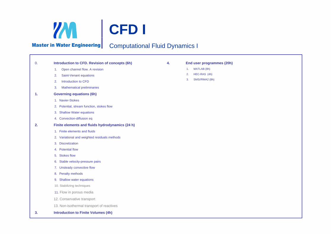
0. Introduction to CFD. Revision of concepts (6h)

1. Open channel flow. A revision

2. Saint-Venant equations

2. Introduction to CFD

3. Mathematical preliminaries

4. End user programmes (20h)1. MATLAB (8h)

2. HEC-RAS (4h)

3. SMS//RMA2 (8h)

1. Governing equations (6h)

1. Navier-Stokes

2. Potential, stream function, stokes flow

3. Shallow Water equations

4. Convection-diffusion eq

2. Finite elements and fluids hydrodynamics (24 h)

1. Finite elements and fluids

2. Variational and weighted residuals methods

3 Discretization3. Discretization

4. Potential flow

5. Stokes flow

6. Stable velocity-pressure pairs

7. Unsteady convective flow

8. Penalty methods

9. Shallow water equations

10. Stabilizing techniques

11. Flow in porous media

12. Conservative transport

13. Non-isothermal transport of reactives

3. Introduction to Finite Volumes (4h)


CFDCFDI 1 Introduction to CFDI 1. Introduction to CFD

CFD I

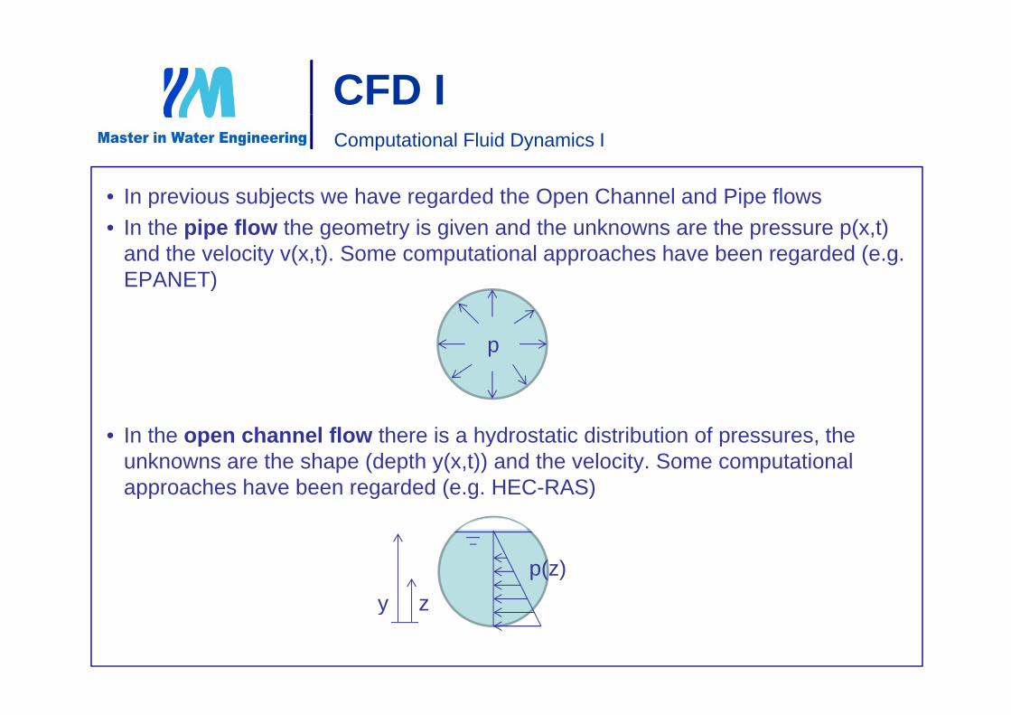
• In previous subjects we have regarded the Open Channel and Pipe flows


• In previous subjects we have regarded the Open Channel and Pipe flows• In the pipe flow the geometry is given and the unknowns are the pressure p(x,t)

and the velocity v(x,t). Some computational approaches have been regarded (e.g. EPANET)EPANET)

p

• In the open channel flow there is a hydrostatic distribution of pressures theIn the open channel flow there is a hydrostatic distribution of pressures, the unknowns are the shape (depth y(x,t)) and the velocity. Some computational approaches have been regarded (e.g. HEC-RAS)

p(z)zy zy


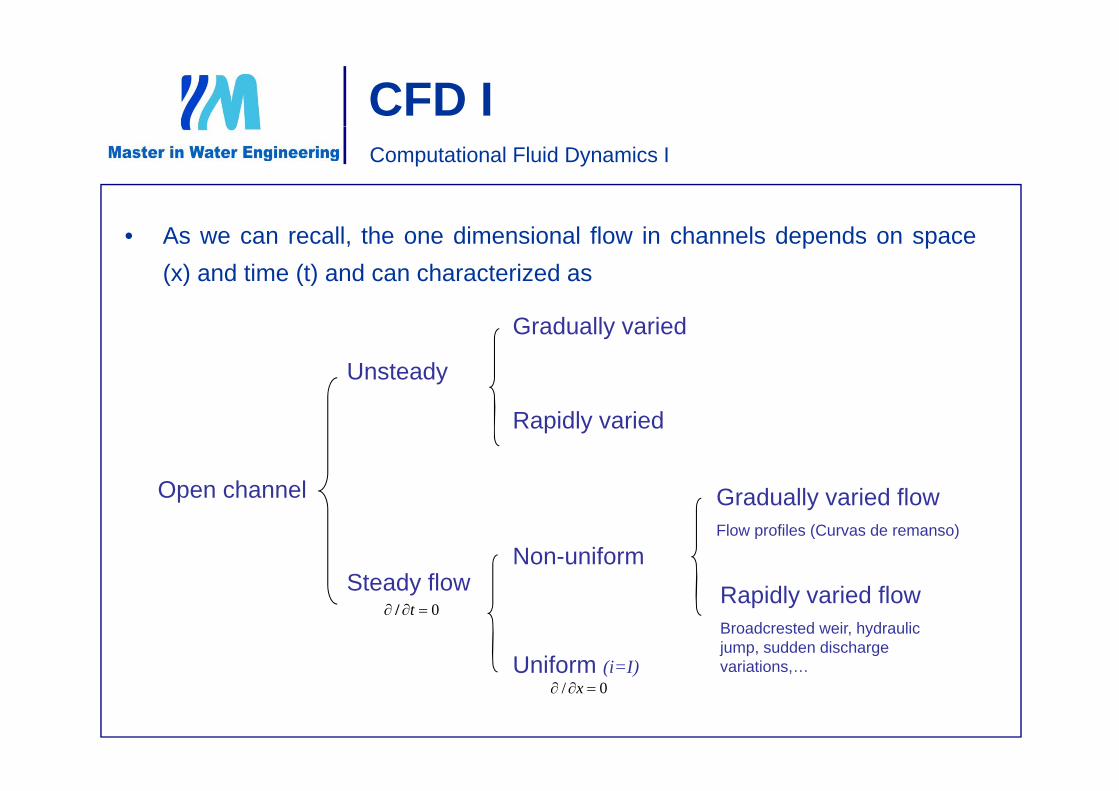
• As we can recall, the one dimensional flow in channels depends on space(x) and time (t) and can characterized as

Gradually varied

Unsteady

Open channel

Rapidly varied

Open channel Gradually varied flowFlow profiles (Curvas de remanso)

Non-uniformSt d fl

Uniform (i=I)

Steady flow Rapidly varied flowBroadcrested weir, hydraulic jump, sudden discharge variations

0 t/

Uniform (i=I) variations,…0/ x

CFD I

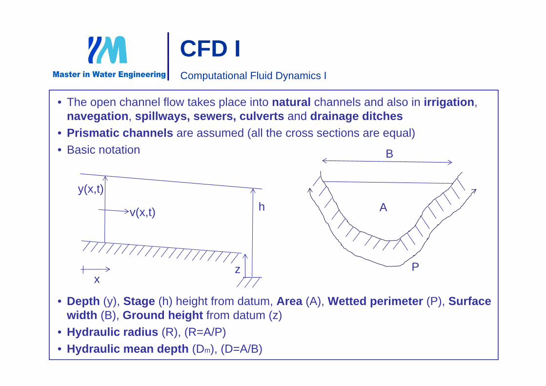
• The open channel flow takes place into natural channels and also in irrigation,


The open channel flow takes place into natural channels and also in irrigation, navegation, spillways, sewers, culverts and drainage ditches

• Prismatic channels are assumed (all the cross sections are equal)• Basic notation B• Basic notation

y(x,t)

B

y( , )

v(x,t) Ah

xPz

• Depth (y), Stage (h) height from datum, Area (A), Wetted perimeter (P), Surface width (B), Ground height from datum (z)

x

• Hydraulic radius (R), (R=A/P)• Hydraulic mean depth (Dm), (D=A/B)

CFD I

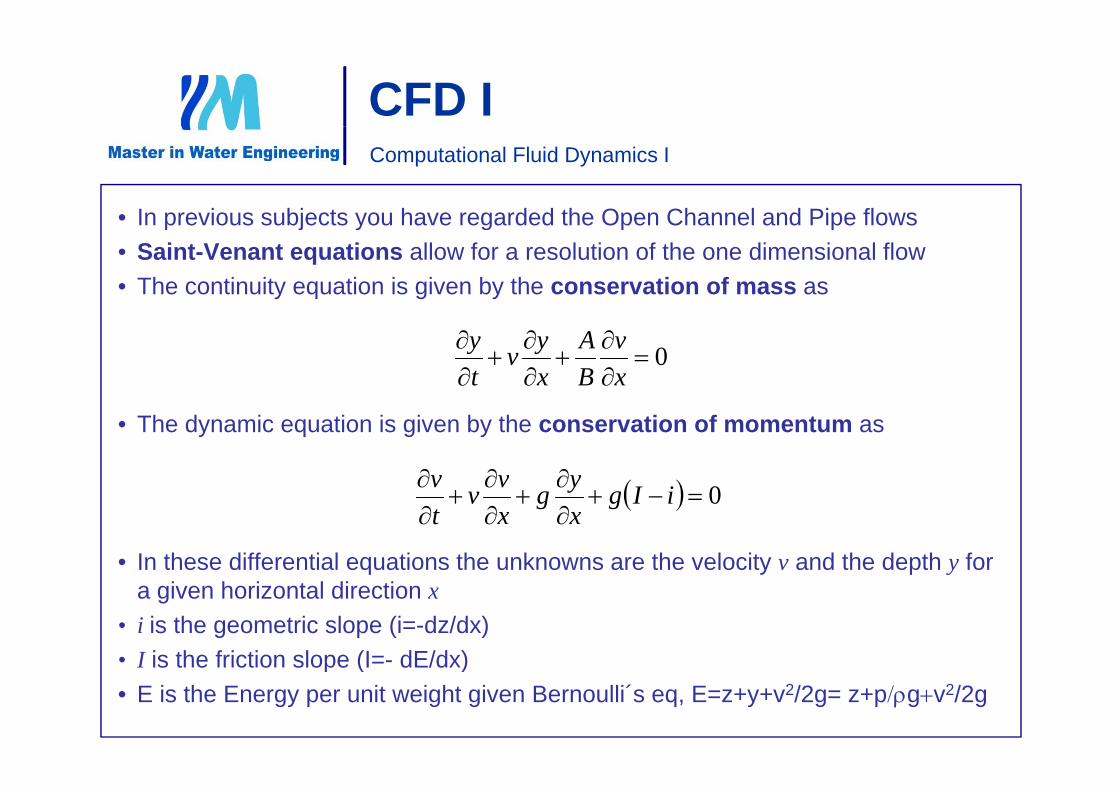
• In previous subjects you have regarded the Open Channel and Pipe flows


• In previous subjects you have regarded the Open Channel and Pipe flows• Saint-Venant equations allow for a resolution of the one dimensional flow• The continuity equation is given by the conservation of mass as

0

xv

BA

xyv

ty

• The dynamic equation is given by the conservation of momentum as

yvv

• In these differential equations the unknowns are the velocity v and the depth y for

0

iIg

xyg

xvv

tv

a given horizontal direction x• i is the geometric slope (i=-dz/dx) • I is the friction slope (I=- dE/dx)I is the friction slope (I dE/dx) • E is the Energy per unit weight given Bernoulli´s eq, E=z+y+v2/2g= z+pgv2/2g

CFD I

• Saint Venant equations assume :


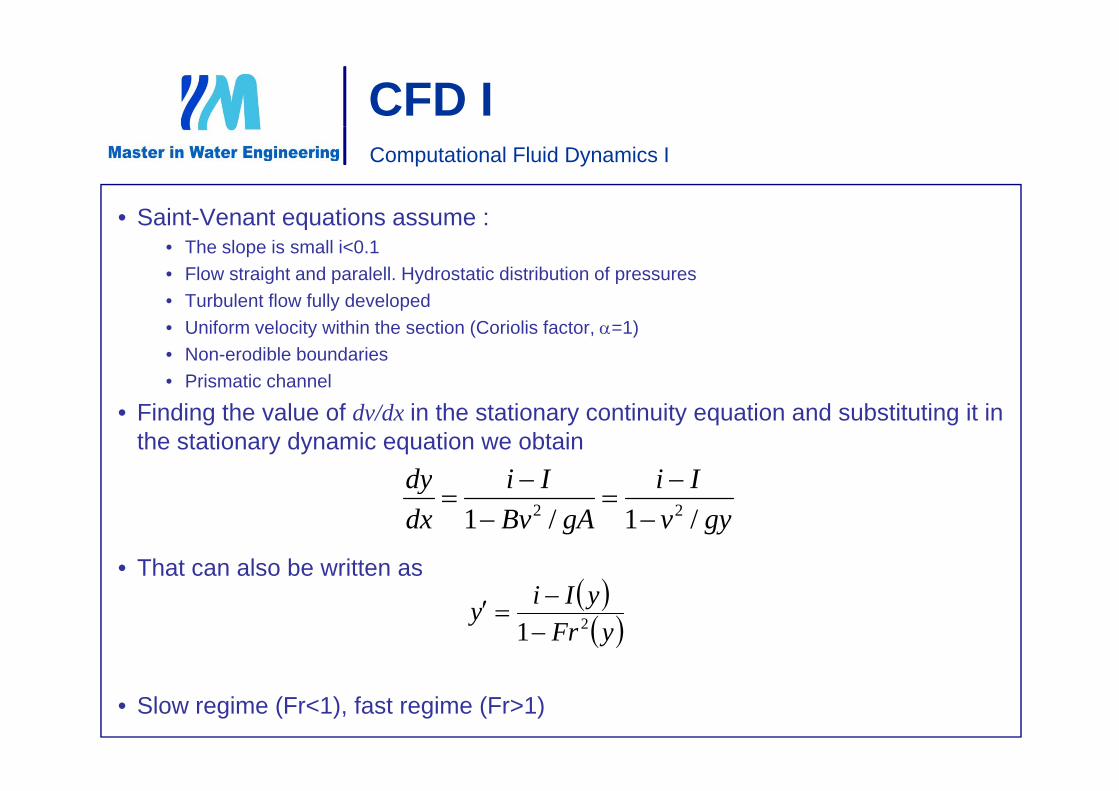
• Saint-Venant equations assume :• The slope is small i<0.1• Flow straight and paralell. Hydrostatic distribution of pressures• Turbulent flow fully developedTurbulent flow fully developed• Uniform velocity within the section (Coriolis factor, =1)• Non-erodible boundaries• Prismatic channel

• Finding the value of dv/dx in the stationary continuity equation and substituting it in the stationary dynamic equation we obtain

IiIidy

• That can also be written as

gyvIi

gABvIi

dxdy

/1/1 22

That can also be written as yFryIiy 21

• Slow regime (Fr<1), fast regime (Fr>1)

CFD I

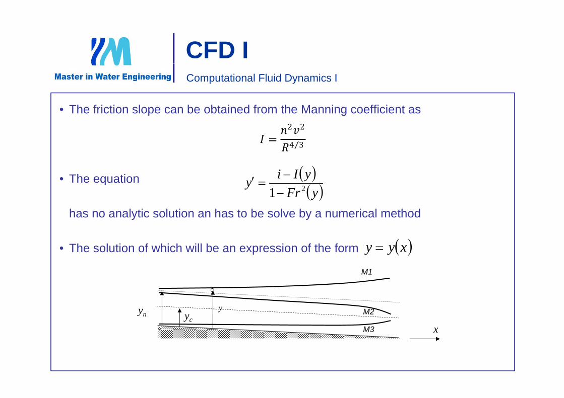
• The friction slope can be obtained from the Manning coefficient as


• The friction slope can be obtained from the Manning coefficient as2 2

4 3⁄

• The equation yFryIiy 21

has no analytic solution an has to be solve by a numerical method

Th l ti f hi h ill b i f th f

y

• The solution of which will be an expression of the form xyy M1

yn y M2

M3 xyc


CFD I

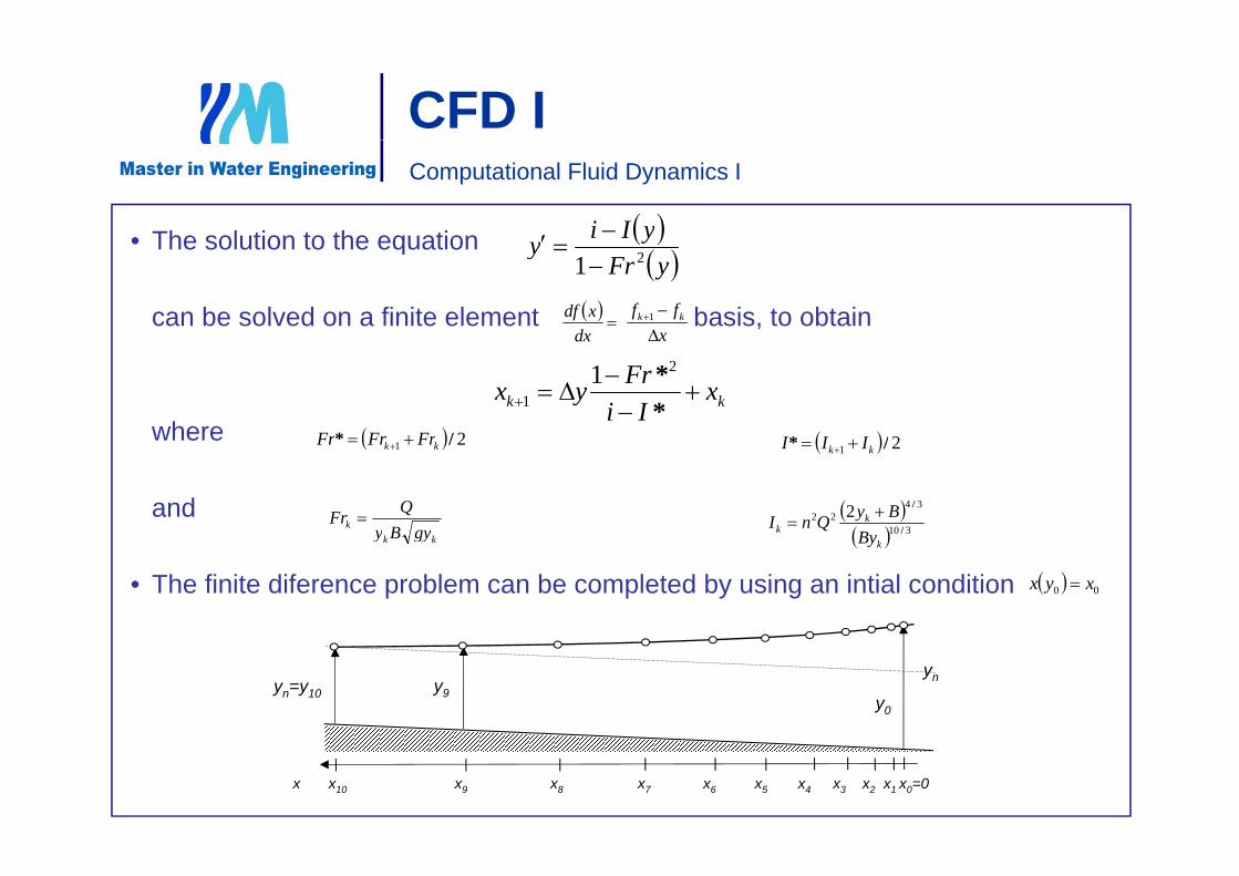
• The solution to the equation


yIi • The solution to the equation

can be solved on a finite element basis, to obtain

yFryy 21

xff kk

1

dx

xdf

wherekk x

IiFryx

**2

11

2/* FrFrFr 2/* III

xdx

where

and

21 /* kk FrFrFr 21 /* kk III

kkk gyBy

QFr 310

3422 2

/

/k

k ByByQnI

• The finite diference problem can be completed by using an intial condition

kk gyBy kBy

00 xyx

yn=y10 y0

y9

yn

x x10 x9 x8 x7 x6 x5 x4 x3 x2 x1 x0=0

CFD I

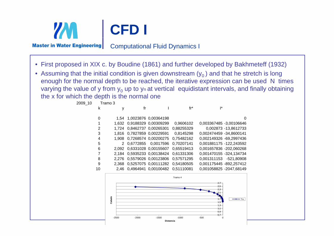
• First proposed in XIX c by Boudine (1861) and further developed by Bakhmeteff (1932)


• First proposed in XIX c. by Boudine (1861) and further developed by Bakhmeteff (1932)• Assuming that the initial condition is given downstream (y0 ) and that he stretch is long

enough for the normal depth to be reached, the iterative expression can be used N times varying the value of y from y0 up to yn at vertical equidistant intervals, and finally obtaining y g y y0 p y q , y gthe x for which the depth is the normal one

2009_10 Tramo 3k y fr I fr* I*

0 1 54 1 0023876 0 00364198 00 1,54 1,0023876 0,00364198 01 1,632 0,9188329 0,00309299 0,9606102 0,003367485 -3,001066462 1,724 0,8462737 0,00265301 0,88255329 0,002873 -13,86127333 1,816 0,7827859 0,00229591 0,8145298 0,002474459 -34,86001414 1,908 0,7268574 0,00200275 0,75482162 0,002149326 -69,29974365 2 0,6772855 0,0017596 0,70207141 0,001881175 -122,2435925 2 0,6772855 0,0017596 0,70207141 0,001881175 122,2435926 2,092 0,6331028 0,00155607 0,65519413 0,001657836 -202,0602687 2,184 0,5935233 0,00138424 0,61331306 0,001470155 -324,1347348 2,276 0,5579026 0,00123806 0,57571295 0,001311153 -521,809089 2,368 0,5257075 0,00111282 0,54180505 0,001175445 -892,257412

10 2,46 0,4964941 0,00100482 0,51110081 0,001058825 -2047,68149

1 71,92,12,32,52,7

do

Tramo 4

T

0,70,91,11,31,51,7

-2500 -2000 -1500 -1000 -500 0

Cal

ad

Distancia

Tra…

CFD I

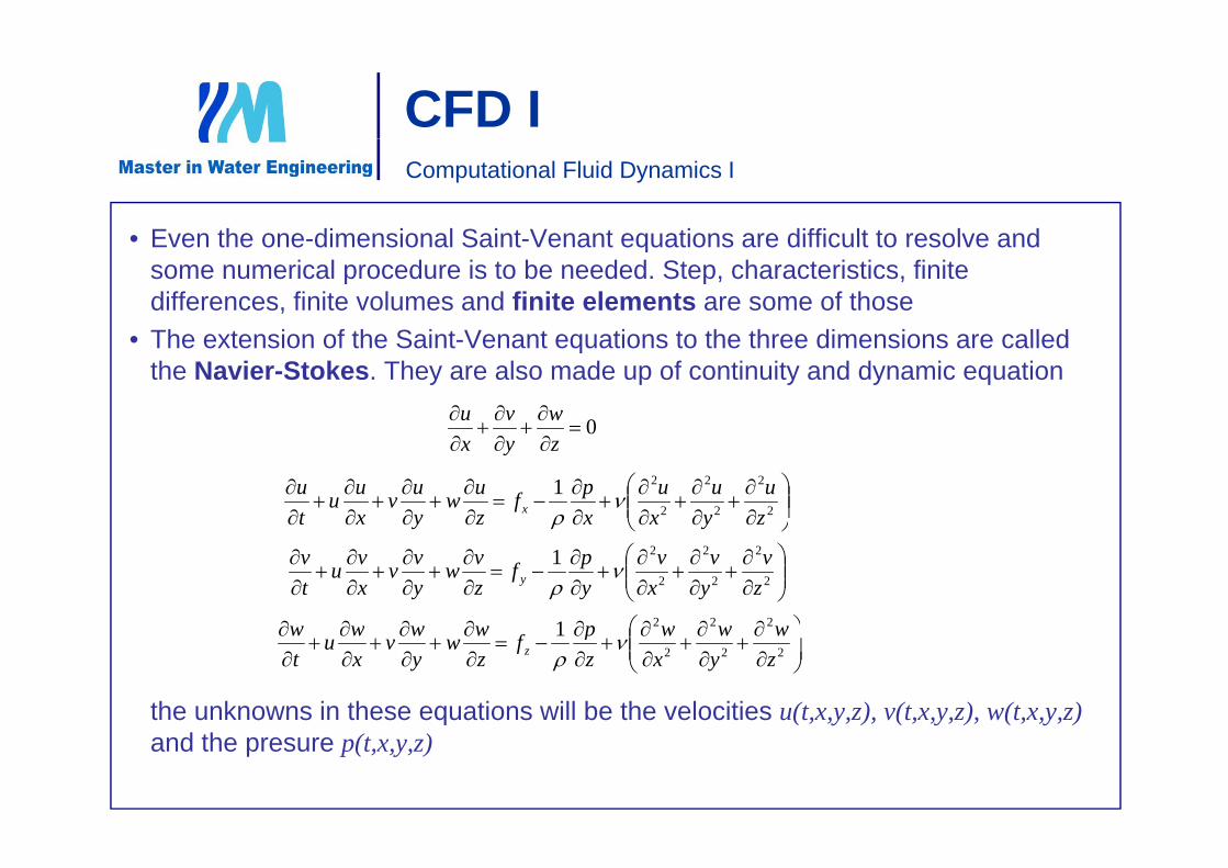
• Even the one dimensional Saint Venant equations are difficult to resolve and


• Even the one-dimensional Saint-Venant equations are difficult to resolve and some numerical procedure is to be needed. Step, characteristics, finite differences, finite volumes and finite elements are some of those

• The extension of the Saint Venant equations to the three dimensions are called• The extension of the Saint-Venant equations to the three dimensions are called the Navier-Stokes. They are also made up of continuity and dynamic equation

0

wvu

zyx

2

2

2

2

2

21zu

yu

xu

xpf

zuw

yuv

xuu

tu

x

2

2

2

2

2

21zv

yv

xv

ypf

zvw

yvv

xvu

tv

y

2221 wwwpwwww

the unknowns in these equations will be the velocities u(t,x,y,z), v(t,x,y,z), w(t,x,y,z)

222

1zw

yw

xw

zpf

zww

ywv

xwu

tw

z

and the presure p(t,x,y,z)

CFD I

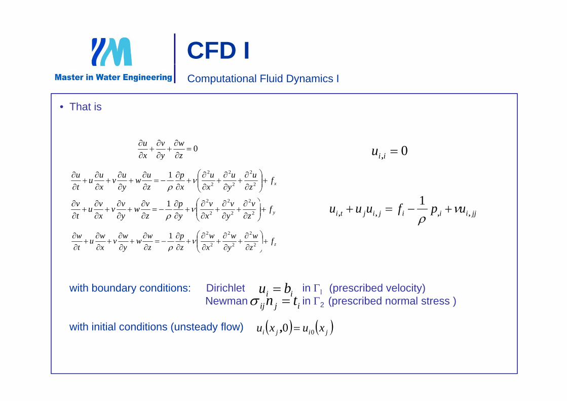
• That is


That is

0

zw

yv

xu

0iiu zyx

xfzu

yu

xu

xp

zuw

yuv

xuu

tu

2

2

2

2

2

21

2221 1

0iiu ,

yfzv

yv

xv

yp

zvw

yvv

xvu

tv

2

2

2

2

2

21

zfwwwpwwwvwutw

2

2

2

2

2

21

jjiiijijti upfuuu ,,,,

1

with boundary conditions: Dirichlet in (prescribed velocity)

zyxzzyxt

222

ii bu t bou da y co d t o s c et (p esc bed e oc ty)Newman in 2 (prescribed normal stress )

with initial conditions (unsteady flow)

ii buijij tn

jiji xuxu 00 ,


• Anyway, in most of the cases some others equations are used to provide a

simplified b t meaningf l sol tion to the flo problems Among these e cansimplified but meaningful solution to the flow problems. Among these we can

quote as some of the most important

–Potential and stream function equations

–Stokes flow eqs.Stokes flow eqs.

–Shallow water flow eqs. (SSWW)


• The potential flow equation is a simplification that uses the potential variable to

solve the continuity equation

• In the stream/vorticity formulation the u and p variables are written in terms of

the variables and , obtaining in this way simplified N-S equations

• In the Stokes equations the convective term is dropped

• The Shallow Water equations are the result of the integration in depth of the

three dimensional equations, therefore a two dimensional model is obtained

CFD I

• The flow in a porous media simplifies Navier-Stokes eq and is also to be


• The flow in a porous media simplifies Navier-Stokes eq. and is also to be

considered

• Once the velocity field is obtained, we can use it as an input value to resolve the

transport equation that gives the concentration of a given species in the flowt a spo t equat o t at g es t e co ce t at o o a g e spec es t e o

• The transport equation can be also considered for non-isothermal reactivesThe transport equation can be also considered for non isothermal reactives

• The equations of the transport of sediments are also needed for the case inThe equations of the transport of sediments are also needed for the case in

which non-soluble substances are included in the flow

• For convective enough flows, a turbulent model is to be required

CFD I

• With respect to the dynamic macroscopic behaviour, flows can be regarded


With respect to the dynamic macroscopic behaviour, flows can be regardedas laminar or turbulent

• The laminar flow is ordered and it takes place in layers• The laminar flow is ordered and it takes place in layers

• In the turbulent flow particles move on an irregular fluctuant and erraticIn the turbulent flow, particles move on an irregular, fluctuant and erraticway -> turbulents models are required

• This situation takes place for a Reynolds number Re(=UL/ > 2000

• The Reynolds number indicates the weight of the convection with respect tothe viscous losses


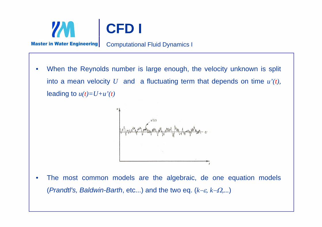
• When the Reynolds number is large enough, the velocity unknown is split

into a mean velocity U and a fluctuating term that depends on time u’(t),

leading to u(t)=U+u’(t)

• The most common models are the algebraic, de one equation models

(Prandtl's Baldwin-Barth etc ) and the two eq (k k )(Prandtl s, Baldwin-Barth, etc...) and the two eq. (k k ,...)


• The FEM was developed in the 50s to be applied to the aeronauticengineering

• Advantages:• Advantages:– Suitable to model complex geometries

– Consistent treatment of b.c.

– Possibility of being programmed in a flexible and general way

• Fluid materials change their shape and that leads to a importantcomplexity

• Structural or heat problems lead to a diffusive equation that turns into affsymetric stiffness matrices

• For those cases, Galerkin formulation leads to convergent iterativesolutions in an easy waysolutions in an easy way


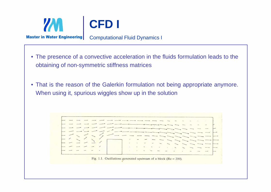
• The presence of a convective acceleration in the fluids formulation leads to theobtaining of non-symmetric stiffness matrices

• That is the reason of the Galerkin formulation not being appropriate anymore.When using it, spurious wiggles show up in the solutiong p gg p


• In order to do avoid these oscillations, some techniques have been developed since the

70s which are known as stabilization techniques. The most important of which are

SUPG (Streamline Upwind Petrov Galerkin)– SUPG (Streamline Upwind Petrov-Galerkin)

– GLS (Galerkin Least Squares)

– FIC (Finite Increment Calculus),...

• A correct coupling in the selection of the pressure and velocity variables is required for

convergenceg

• The heterogeneity of the unknowns require the use of the so-called mixed and penalized

methodsmethods

• The mesh refinement also leads to the stabilization (but means high computational costs

index

0. Introduction to CFD (4 h)


0. Introduction to CFD (4 h)

1. Governing equations (6 h)

1. Navier-Stokes

2. Potential, stream function, stokes flow

3. Shallow Water equations

4. Convection-diffusion eq

2. Finite elements and fluids hydrodynamics (26 h)

1. Finite elements and fluids

2. Variational and weighted residuals methods

3. Discretization

4. Potential flow

5. Stokes flow

6. Stable velocity-pressure pairs

7 Unsteady convective flow7. Unsteady convective flow

8. Penalty methods

9. Shallow water equations

10. Stabilizing techniques

3. Flow in porous media (6 h)

4. Conservative transport (6 h)

• Non-isothermal transport of reactives

• Transport of sediments

• Turbulence models

• Finite volumes

introduction to CFDderivative operators

f ( ) i 1D l fi ld

derivative operatorscomputational fluid dynamics I

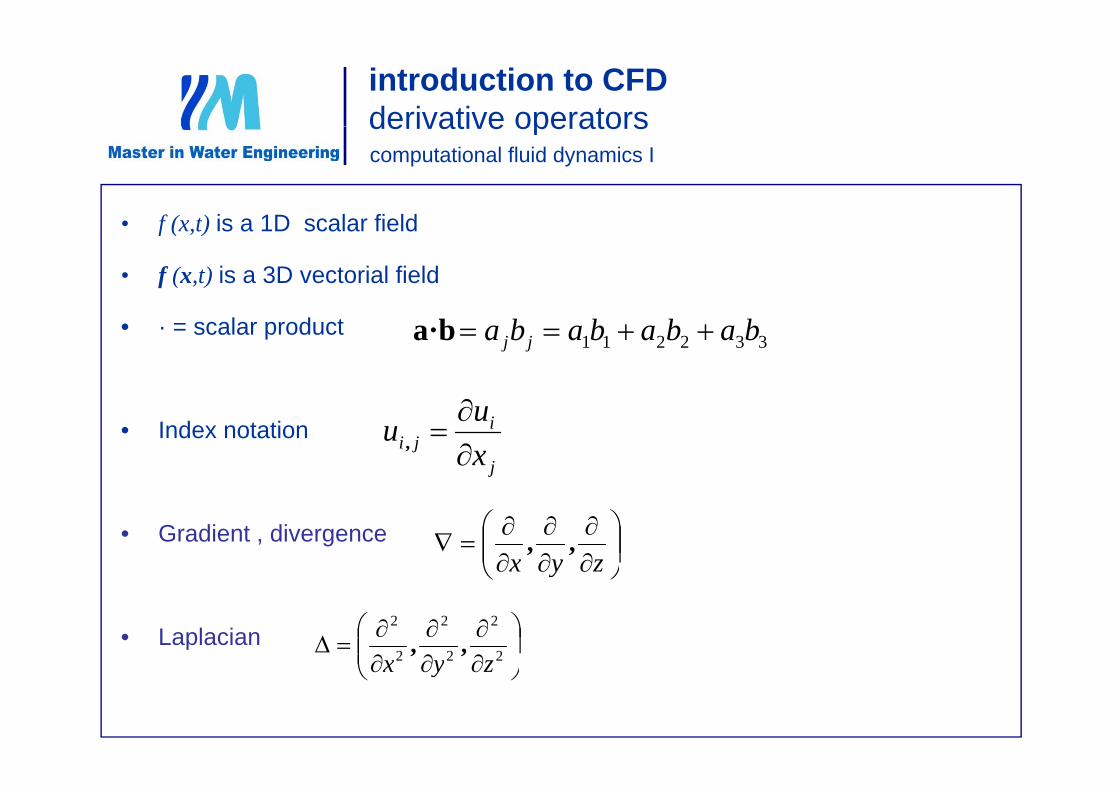
• f (x,t) is a 1D scalar field

• f (x,t) is a 3D vectorial field

• · = scalar product332211 babababa jj a·b

• Index notationj

iji x

uu

,

• Gradient , divergence

zyx

,,

• Laplacian

y

2

2

2

2

2

2

zyx,,

zyx

introduction to CFDReference SystemReference Systemcomputational fluid dynamics I

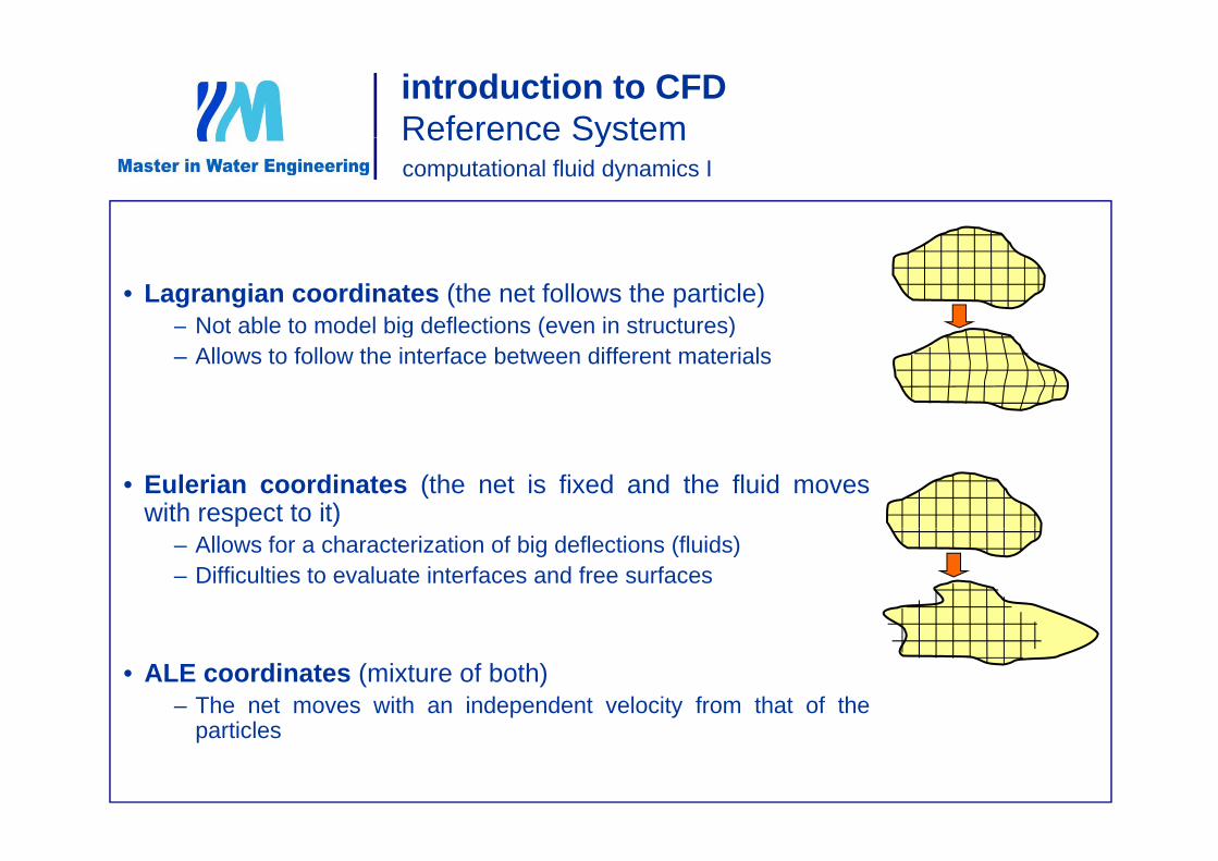
• Lagrangian coordinates (the net follows the particle)– Not able to model big deflections (even in structures)Not able to model big deflections (even in structures)– Allows to follow the interface between different materials

• Eulerian coordinates (the net is fixed and the fluid moveswith respect to it)

– Allows for a characterization of big deflections (fluids)– Difficulties to evaluate interfaces and free surfaces

• ALE coordinates (mixture of both)– The net moves with an independent velocity from that of the

ti lparticles

introduction to CFDeulerian coordinateseulerian coordinatescomputational fluid dynamics I

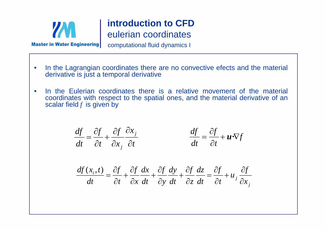
• In the Lagrangian coordinates there are no convective efects and the materialderivative is just a temporal derivative

I th E l i di t th i l ti t f th t i l• In the Eulerian coordinates there is a relative movement of the materialcoordinates with respect to the spatial ones, and the material derivative of anscalar field f is given by

xffddf j

ftf

dtdf

·utxtdt j

ftdt

ffdfdfdffdf )(

jj

i

xfu

tf

dtdz

zf

dtdy

yf

dtdx

xf

tf

dttxdf

),(


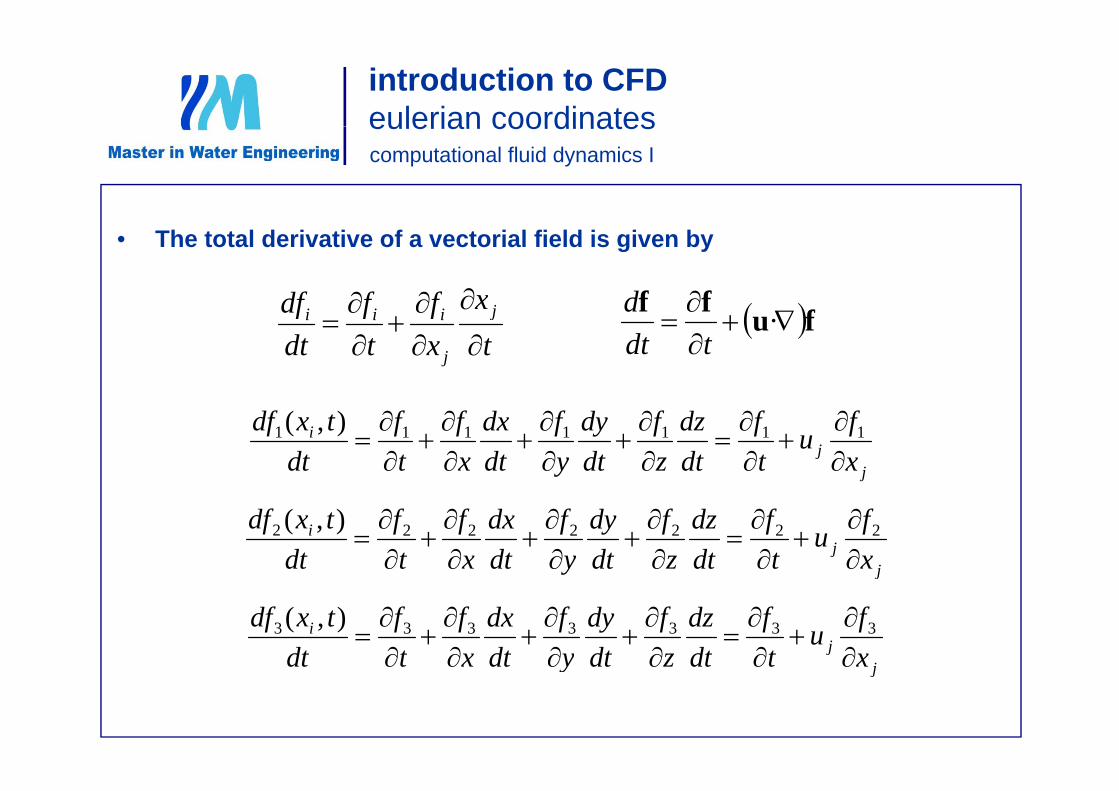
• The total derivative of a vectorial field is given by

xffdf j ff dt

xxf

tf

dtdf j

j

iii

fuff

·tdt

d

jj

i

xfu

tf

dtdz

zf

dtdy

yf

dtdx

xf

tf

dttxdf

1111111 ),(

jj

i

xfu

tf

dtdz

zf

dtdy

yf

dtdx

xf

tf

dttxdf

2222222 ),(

j

jj

i

xfu

tf

dtdz

zf

dtdy

yf

dtdx

xf

tf

dttxdf

3333333 ),(

jxtdtzdtydtxtdt


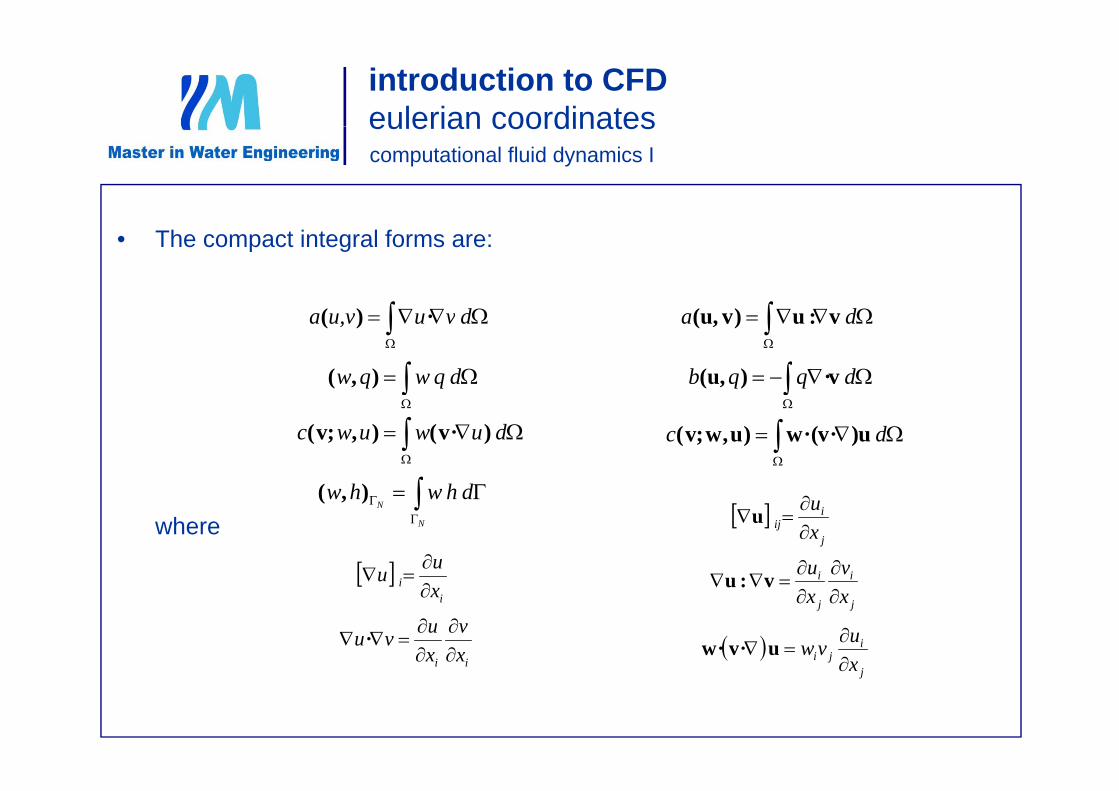
• The compact integral forms are:

da v:u)vu,(

dqqb v·)u,(

dvuu,va ·)(

dqwqw ),(

dc u)·v·(w)u,w;v(

duwuwc )·v(),;v(

dhh)(where

j

iij x

u

u

ii vu uu

dhwhwN

N),(

j

i

j

i

xx v:u

iji x

uvw

u·v·w

i

i xu

ii xv

xuvu

·jxii

governing equations

computational fluid dynamics I

CFDCFDI2 Governing EquationsI2. Governing Equations

governing equationsstress() and strain() of fluids

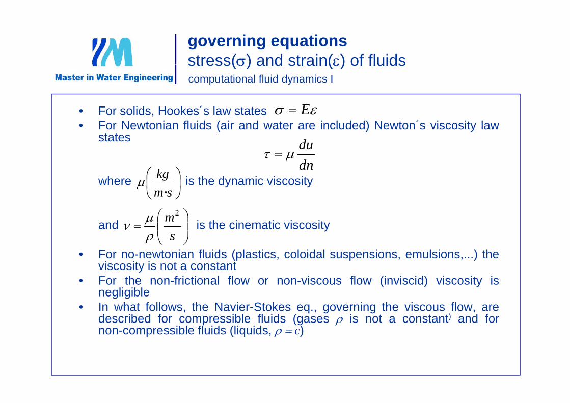
• For solids Hookes´s law states

stress() and strain() of fluidscomputational fluid dynamics I

E• For solids, Hookes s law states• For Newtonian fluids (air and water are included) Newton´s viscosity law

states

E

du

where is the dynamic viscositydn

smkg·

and is the cinematic viscosity

sm2

• For no-newtonian fluids (plastics, coloidal suspensions, emulsions,...) theviscosity is not a constant

• For the non-frictional flow or non-viscous flow (inviscid) viscosity isnegligiblenegligible

• In what follows, the Navier-Stokes eq., governing the viscous flow, aredescribed for compressible fluids (gases is not a constant) and fornon-compressible fluids (liquids, c)

governing equationscontinuity equation

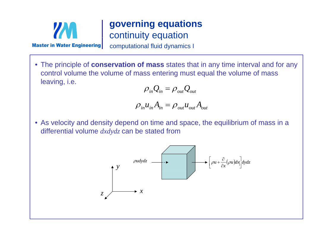
• The principle of conservation of mass states that in any time interval and for any

continuity equationcomputational fluid dynamics I

• The principle of conservation of mass states that in any time interval and for any control volume the volume of mass entering must equal the volume of mass leaving, i.e.

outoutinin QQ outoutinin QQ

outoutoutininin AuAu

• As velocity and density depend on time and space, the equilibrium of mass in a differential volume dxdydz can be stated from

dydzdxux

u

udydzy

xz

governing equationscontinuity equation

• The flux of mass per second this is is equal to (subtract in figure)

continuity equationcomputational fluid dynamics I

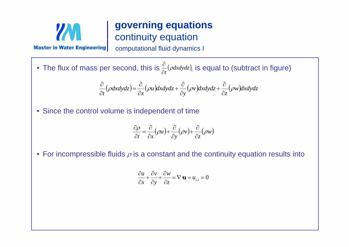
dxdydz• The flux of mass per second, this is , is equal to (subtract in figure) dxdydzt

dxdydzwz

dxdydzvy

dxdydzux

dxdydzt

• Since the control volume is independent of time

y

F i ibl fl id i t t d th ti it ti lt i t

wz

vy

uxt

• For incompressible fluids is a constant and the continuity equation results into

0

iiuwvu u· iizyx ,

governing equationsdynamic equation

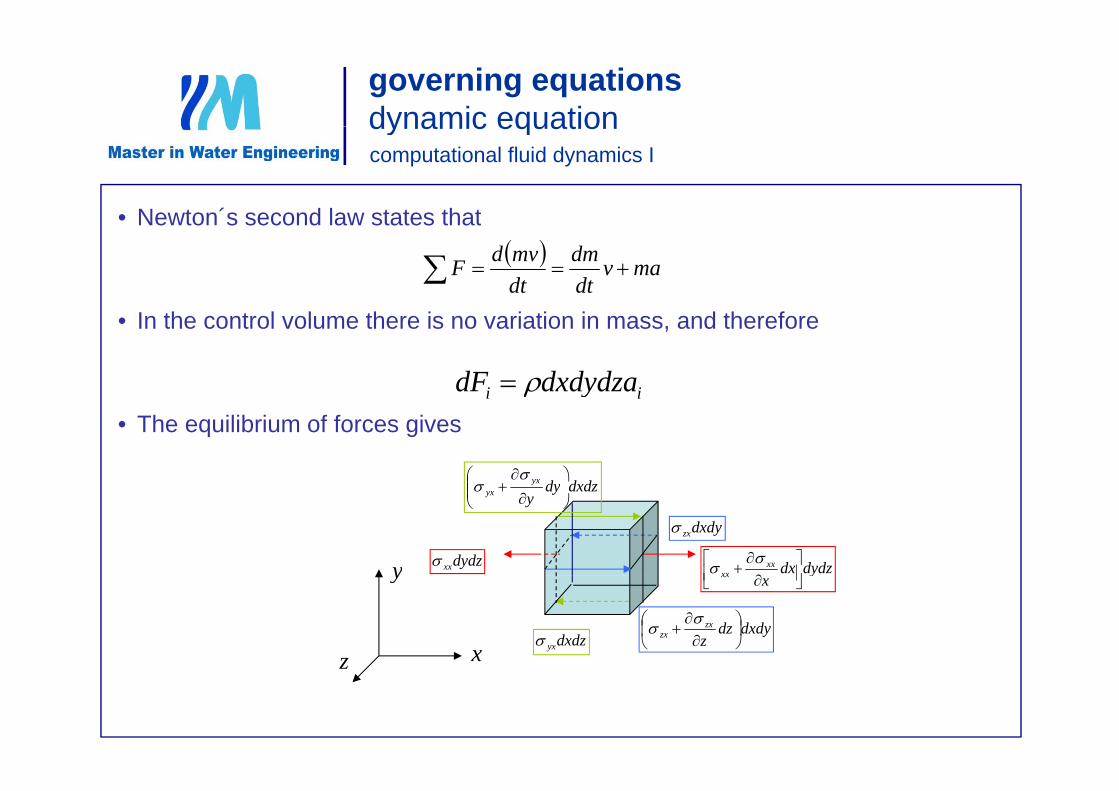
• Newton´s second law states that

dynamic equationcomputational fluid dynamics I

• Newton s second law states that mav

dtdm

dtmvdF

• In the control volume there is no variation in mass, and therefore

ii dxdydzadF • The equilibrium of forces gives

ii y

dxdzdyyx

dydzdxxxxx

y dydzxx

dxdyzx

dxdzdyyyx

yxxx

xz

y

dxdydzz

zxzx

dxdzyxz


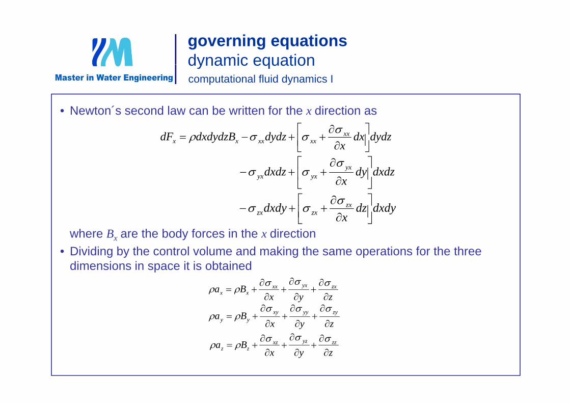
• Newton´s second law can be written for the x direction as


• Newton s second law can be written for the x direction as

dydzdxx

dydzdxdydzBdF xxxxxxxx

dxdzdyx

dxdz yxyxyx

where Bx are the body forces in the x directionDi idi b th t l l d ki th ti f th th

dxdydzx

dxdy zxzxzx

• Dividing by the control volume and making the same operations for the three dimensions in space it is obtained

Ba zxyxxxxx

zyxxx

zyxBa zyyyxy

yy

zyx

Ba zzyzxzzz

governing equationsstresses in solids

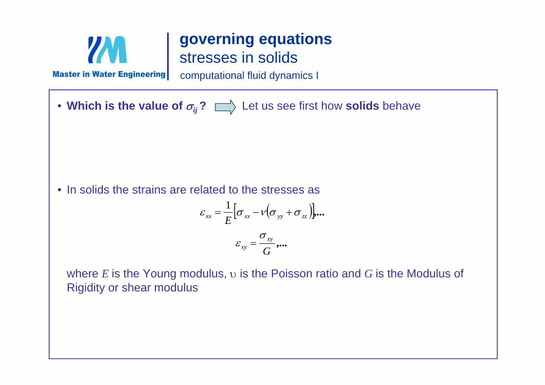
• Which is the value of ? Let us see first how solids behave

stresses in solidscomputational fluid dynamics I

• Which is the value of ij ? Let us see first how solids behave

• In solids the strains are related to the stresses asIn solids the strains are related to the stresses as

,...zzyyxxxx E

1

where E is the Young modulus, is the Poisson ratio and G is the Modulus of

,...G

xyxy

Rigidity or shear modulus


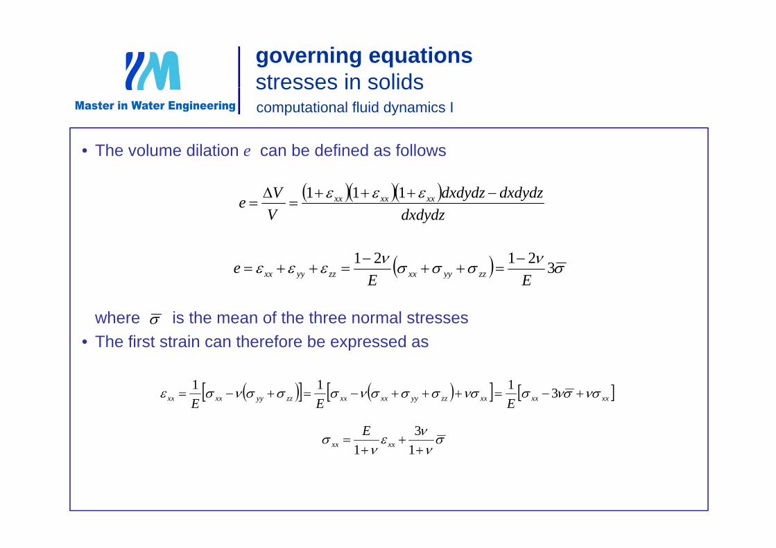
• The volume dilation e can be defined as follows


• The volume dilation e can be defined as follows

d d d

dxdydzdxdydzVVe xxxxxx

111dxdydzV

32121e zzyyxxzzyyxx

where is the mean of the three normal stressesTh fi t t i th f b d

EE zzyyxxzzyyxx

• The first strain can therefore be expressed as

xxxxxxzzyyxxxxzzyyxxxx 3111 xxxxxxzzyyxxxxzzyyxxxx EEE

13

1 xxxxE

governing equationsstresses in solidsstresses in solidscomputational fluid dynamics I

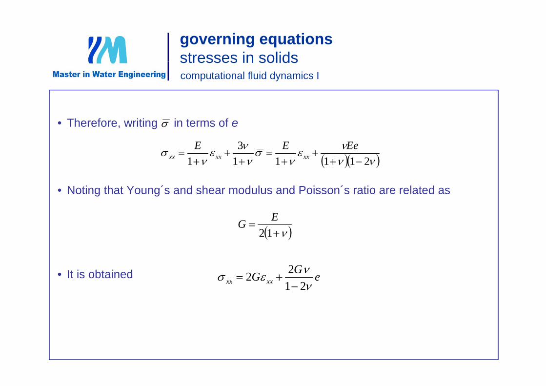
• Therefore, writing in terms of e

3 EeEE

• Noting that Young´s and shear modulus and Poisson´s ratio are related as

211111

xxxxxx

Noting that Young s and shear modulus and Poisson s ratio are related as

12EG

• It is obtained

eGG xxxx 22 eG xxxx

21


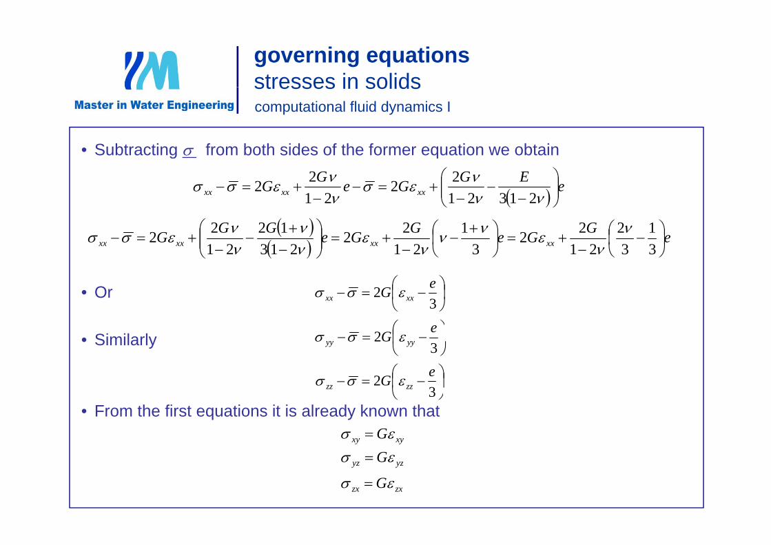
• Subtracting from both sides of the former equation we obtain


• Subtracting from both sides of the former equation we obtain

eEGGeGG xxxxxx

2132122

2122

eGGeGGeGGG xxxxxxxx

31

32

2122

31

2122

21312

2122

• Or

Si il l

32 eG xxxx

2 eG• Similarly

3

2G yyyy

32 eG zzzz

• From the first equations it is already known that 3

xyxy G

G yzyz G

zxzx G

governing equationsstresses in fluidsstresses in fluidscomputational fluid dynamics I

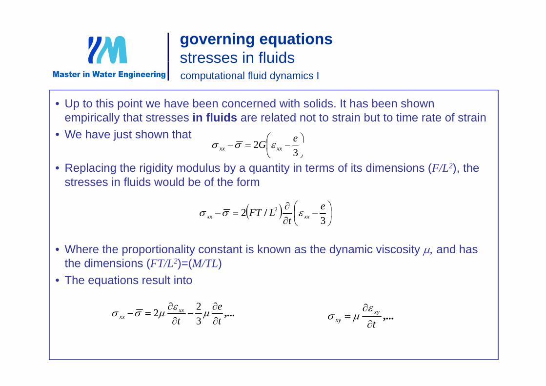
• Up to this point we have been concerned with solids It has been shownUp to this point we have been concerned with solids. It has been shown empirically that stresses in fluids are related not to strain but to time rate of strain

• We have just shown that

32 eG xxxx

• Replacing the rigidity modulus by a quantity in terms of its dimensions (F/L2), the stresses in fluids would be of the form

3xxxx

3

2 2 et

LFT xxxx /

• Where the proportionality constant is known as the dynamic viscosity and has the dimensions (FT/L2)=(M/TL)

• The equations result into• The equations result into

,...te

txx

xx

322 ,...

txy

xy

t


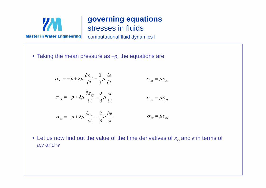
• Taking the mean pressure as –p, the equations are

te

tp xx

xx

322 xyxy

e 2te

tp yy

yy

322

ezz 22

yzyz

L t fi d t th l f th ti d i ti f d i t f

ttp zz

zz

32 zxzx

• Let us now find out the value of the time derivatives of xy and e in terms of u,v and w


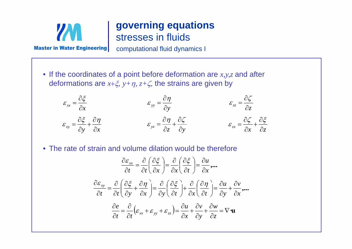
• If the coordinates of a point before deformation are x,y,z and after deformations are xy+, z+the strains are given by

xxx

yyy

zzz

• The rate of strain and volume dilation would be therefore

xyxy

yzyz

zxzx

,...xu

txxttxx

wvue

,...xv

yu

txtyxyttxy

u·

zyxtt zzyyxx


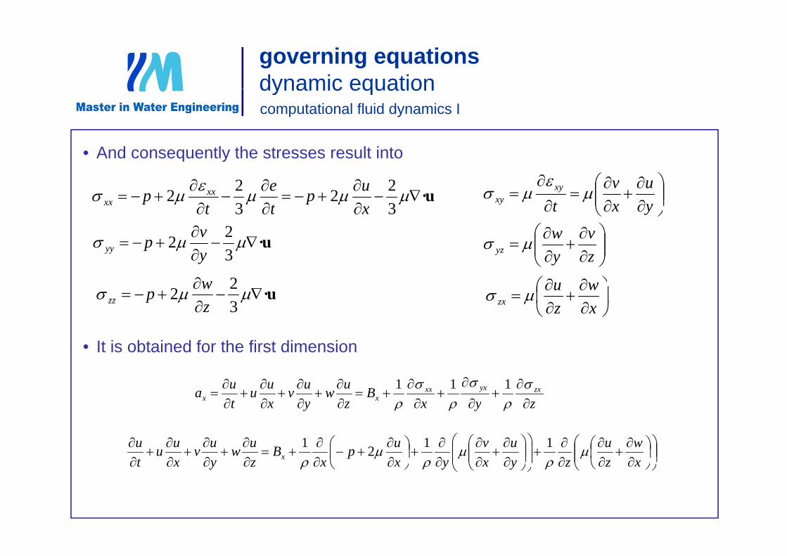
• And consequently the stresses result into


• And consequently the stresses result into

u·

322

322

xup

te

tp xx

xx

yu

xv

txy

xy

u·

322

yvpyy

2

zv

yw

yz

It i bt i d f th fi t di i

u·

322

zwpzz

xw

zu

zx

• It is obtained for the first dimension

zyxB

zuw

yuv

xuu

tua zxyxxx

xx

111

zyxzyxt

xw

zu

zyu

xv

yxup

xB

zuw

yuv

xuu

tu

x

1121 yyy


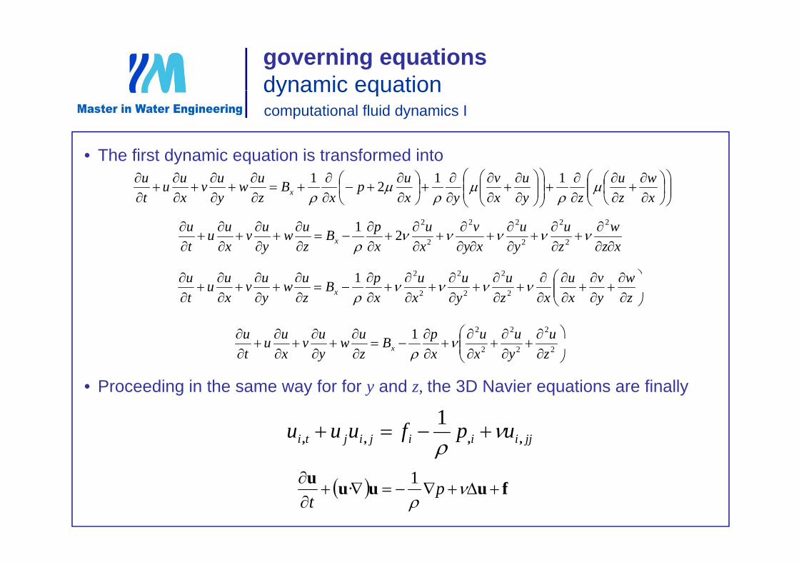
• The first dynamic equation is transformed into


• The first dynamic equation is transformed into

xw

zu

zyu

xv

yxup

xB

zuw

yuv

xuu

tu

x

1121

xzw

zu

yu

xyv

xu

xpB

zuw

yuv

xuu

tu

x

2

2

2

2

22

2

2

21

wvuuuupBuuuu 2221

zyxxzyxx

pBz

wy

vx

ut x

222

2

2

2

2

2

21 uuupBuwuvuuu

• Proceeding in the same way for for y and z, the 3D Navier equations are finally

1

222 zyxx

Bz

wy

vx

ut x

jjiiijijti upfuuu ,,,,

1

1 fuuuu

p

t1·


• That is


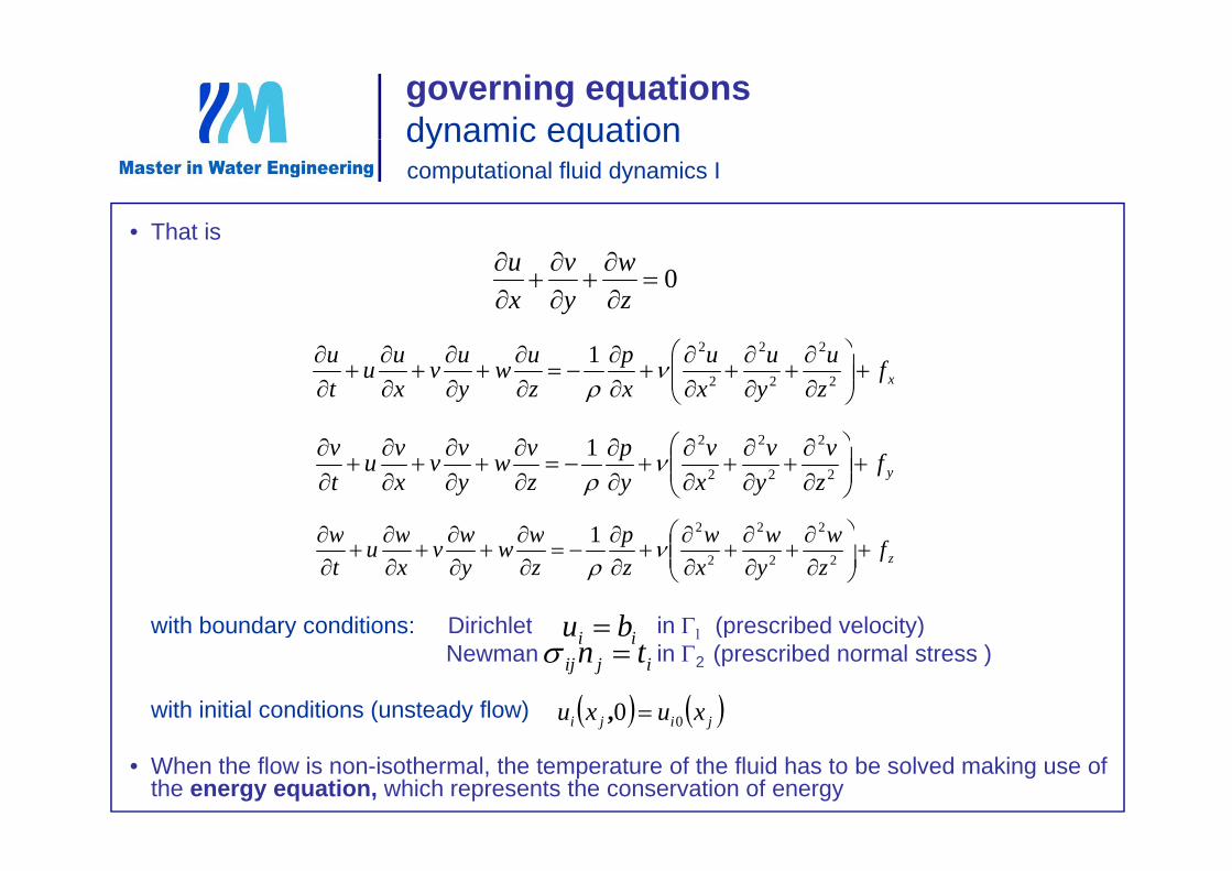
That is

0

zw

yv

xu

xfzu

yu

xu

xp

zuw

yuv

xuu

tu

2

2

2

2

2

21

222

yfzv

yv

xv

yp

zvw

yvv

xvu

tv

2

2

2

2

2

21

wwwpwwww

2221

with boundary conditions: Dirichlet in (prescribed velocity)

zfzw

yw

xw

zp

zww

ywv

xwu

tw

222

1

ii bu t bou da y co d t o s c et (p esc bed e oc ty)Newman in 2 (prescribed normal stress )

with initial conditions (unsteady flow)

ii buijij tn

jiji xuxu 00 ,

• When the flow is non-isothermal, the temperature of the fluid has to be solved making use of the energy equation, which represents the conservation of energy

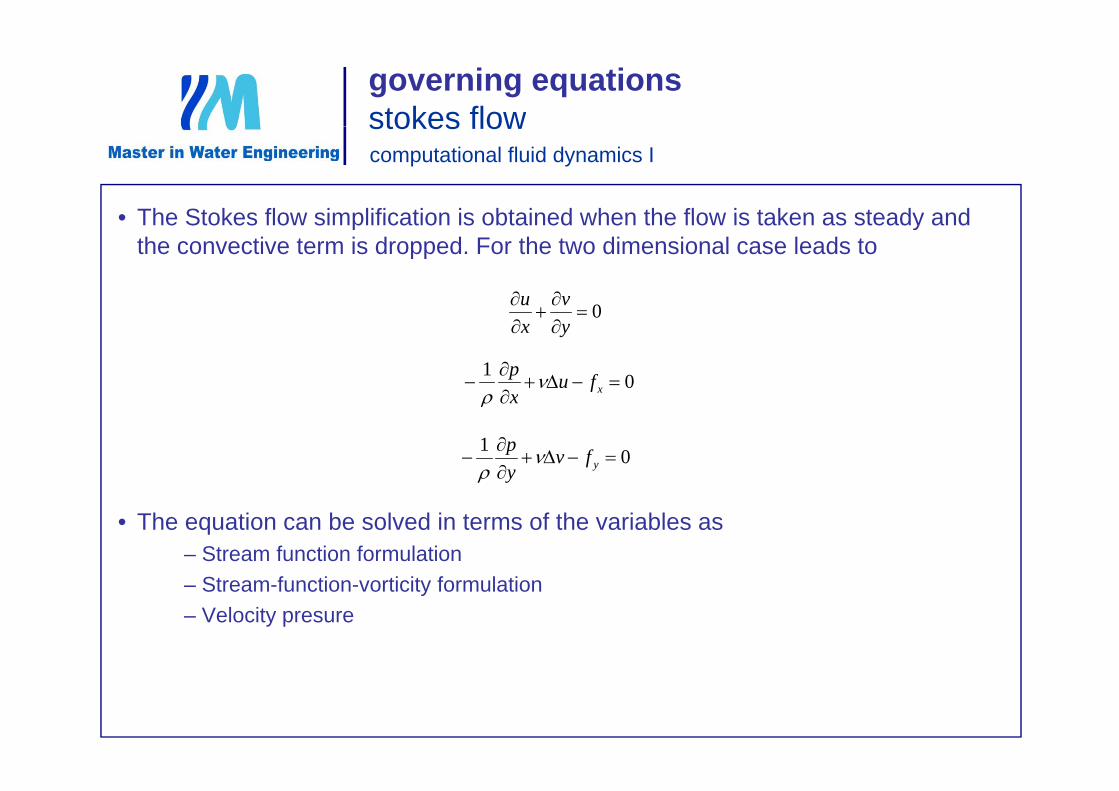
governing equationsstokes flow

• The Stokes flow simplification is obtained when the flow is taken as steady and

stokes flowcomputational fluid dynamics I

• The Stokes flow simplification is obtained when the flow is taken as steady and the convective term is dropped. For the two dimensional case leads to

0 vu

01

xfuxp

0

yx

x

01

yfvyp

• The equation can be solved in terms of the variables as – Stream function formulation– Stream-function-vorticity formulation– Velocity presure

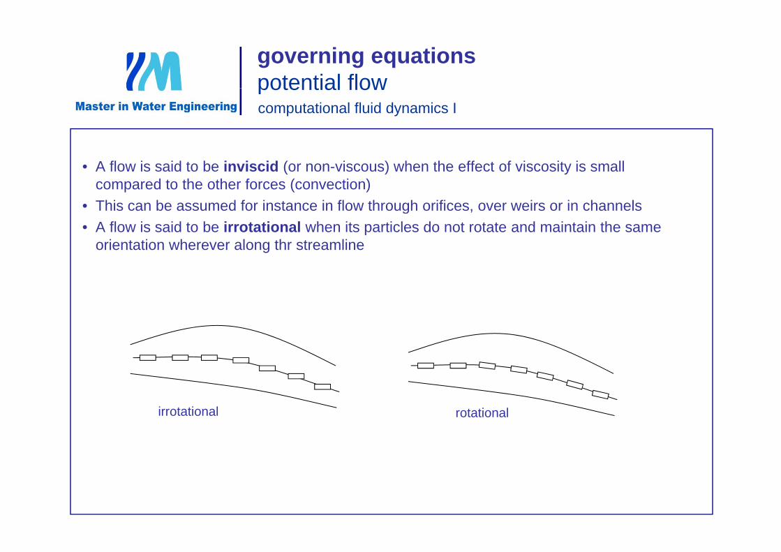
governing equationspotential flowpotential flowcomputational fluid dynamics I

• A flow is said to be inviscid (or non-viscous) when the effect of viscosity is small compared to the other forces (convection)

• This can be assumed for instance in flow through orifices, over weirs or in channelsg• A flow is said to be irrotational when its particles do not rotate and maintain the same

orientation wherever along thr streamline

irrotational rotational

governing equationspotential flowpotential flowcomputational fluid dynamics I

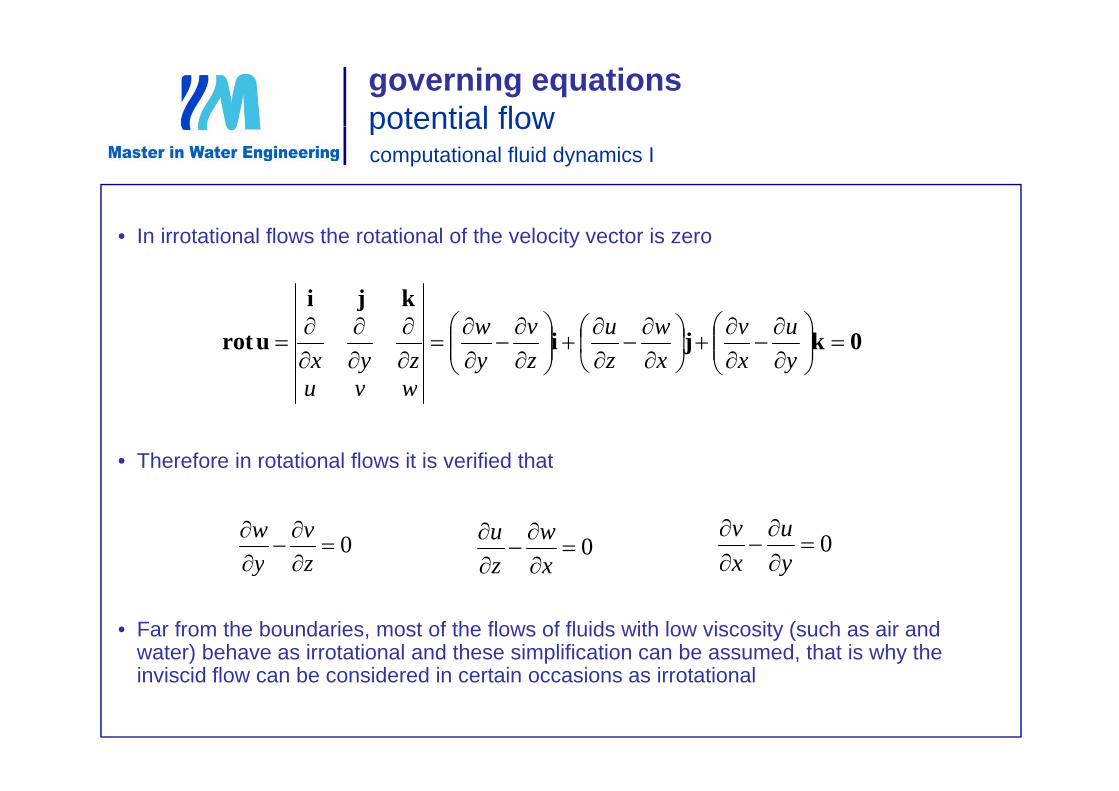
• In irrotational flows the rotational of the velocity vector is zero

kji

0kji

kji

urot

yu

xv

xw

zu

zv

yw

wvuzyx

• Therefore in rotational flows it is verified that

wvu

0

zv

yw

0

xw

zu 0

yu

xv

• Far from the boundaries, most of the flows of fluids with low viscosity (such as air and water) behave as irrotational and these simplification can be assumed, that is why the

y y

inviscid flow can be considered in certain occasions as irrotational

governing equationspotential flow

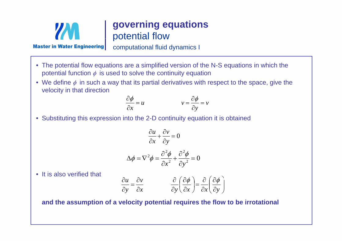
• The potential flow equations are a simplified version of the N-S equations in which the

potential flowcomputational fluid dynamics I

• The potential flow equations are a simplified version of the N-S equations in which the potential function is used to solve the continuity equation

• We define in such a way that its partial derivatives with respect to the space, give the velocity in that directiony

• Substituting this expression into the 2-D continuity equation it is obtained

ux

v

yv

g p y q

0

yv

xu

• It is also verified that

02

2

2

22

yx

It is also verified that

and the assumption of a velocity potential requires the flow to be irrotational

xv

yu

yxxy

and the assumption of a velocity potential requires the flow to be irrotational

governing equationspotential flow

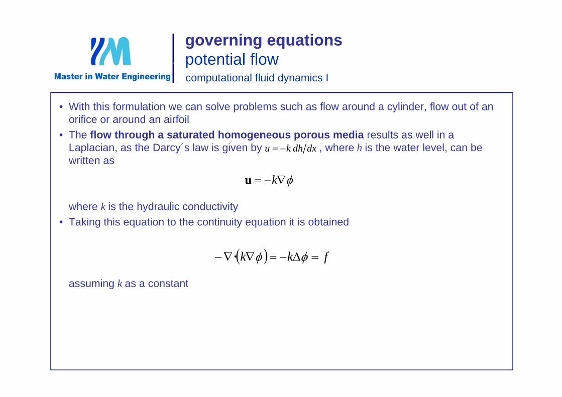
• With this formulation we can solve problems such as flow around a cylinder flow out of an

potential flow computational fluid dynamics I

With this formulation we can solve problems such as flow around a cylinder, flow out of an orifice or around an airfoil

• The flow through a saturated homogeneous porous media results as well in a Laplacian, as the Darcy´s law is given by , where h is the water level, can be dxdhku written as

ku

where k is the hydraulic conductivity• Taking this equation to the continuity equation it is obtained

assuming k as a constant

fkk ·

g

governing equationspotential flowpotential flowcomputational fluid dynamics 1

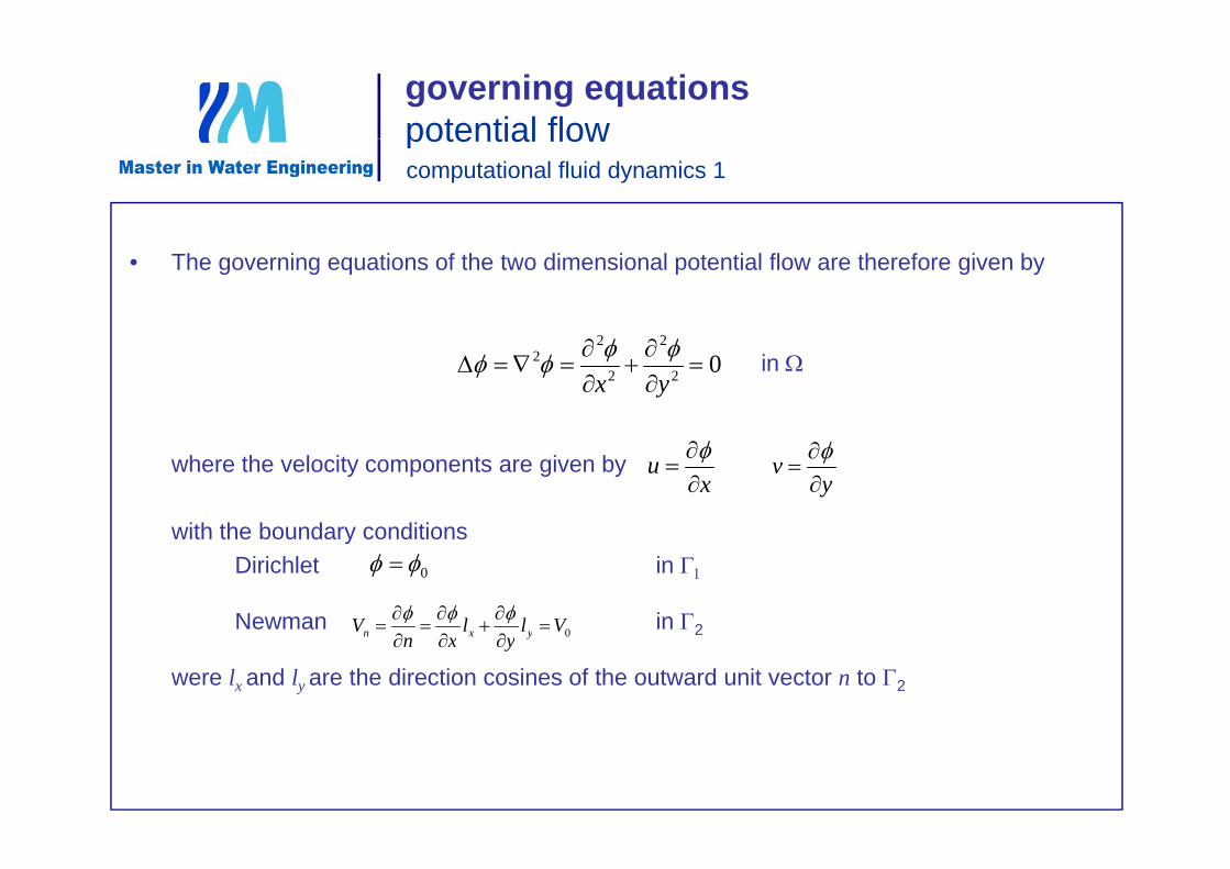
• The governing equations of the two dimensional potential flow are therefore given by

22

in 02

2

2

22

yx

where the velocity components are given by

with the boundary conditions

xu

yv

with the boundary conditionsDirichlet in

Newman in 2

0

0VllV yxn

2

were lx and ly are the direction cosines of the outward unit vector n to 2

0yxn yxn

governing equationsstream functionstream function computational fluid dynamics 1

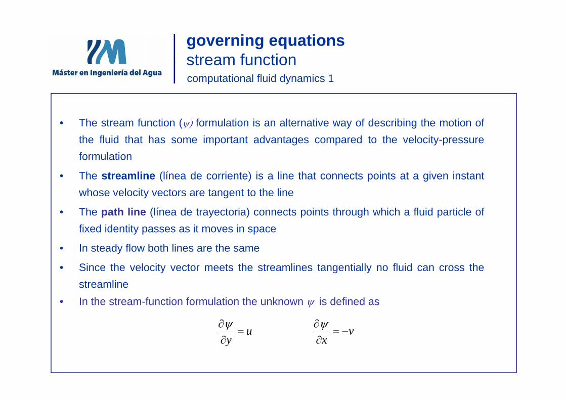
• The stream function ( formulation is an alternative way of describing the motion ofthe fluid that has some important advantages compared to the velocity-pressureformulationformulation

• The streamline (línea de corriente) is a line that connects points at a given instantwhose velocity vectors are tangent to the line

• The path line (línea de trayectoria) connects points through which a fluid particle offixed identity passes as it moves in space

I t d fl b th li th• In steady flow both lines are the same

• Since the velocity vector meets the streamlines tangentially no fluid can cross thestreamline

• In the stream-function formulation the unknown is defined as

u v

y x

governing equationsstream function

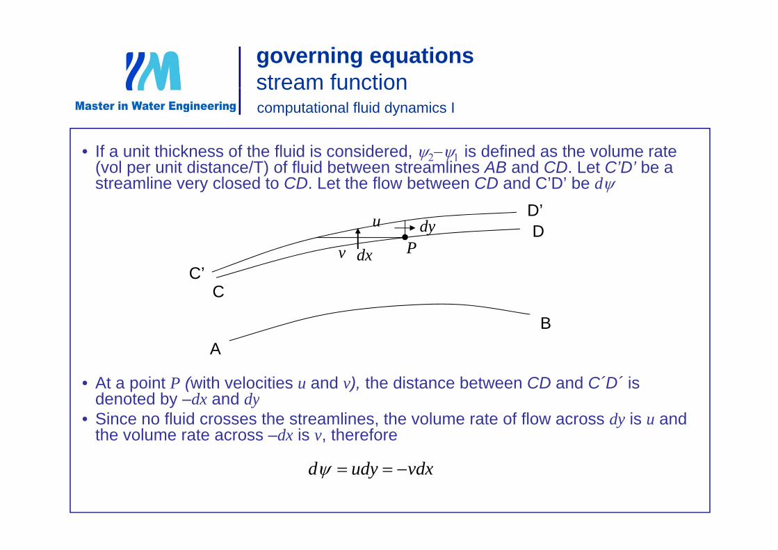
• If a unit thickness of the fluid is considered is defined as the volume rate

stream function computational fluid dynamics I

• If a unit thickness of the fluid is considered, is defined as the volume rate (vol per unit distance/T) of fluid between streamlines AB and CD. Let C’D’ be a streamline very closed to CD. Let the flow between CD and C’D’ be d

D’

C’

Ddx

dyv

u D

PC

C

B

• At a point P (with velocities u and v), the distance between CD and C´D´ is denoted by –dx and dy

A

denoted by –dx and dy• Since no fluid crosses the streamlines, the volume rate of flow across dy is u and

the volume rate across –dx is v, therefore

ddd vdxudyd

governing equationsstream functionstream function computational fluid dynamics I

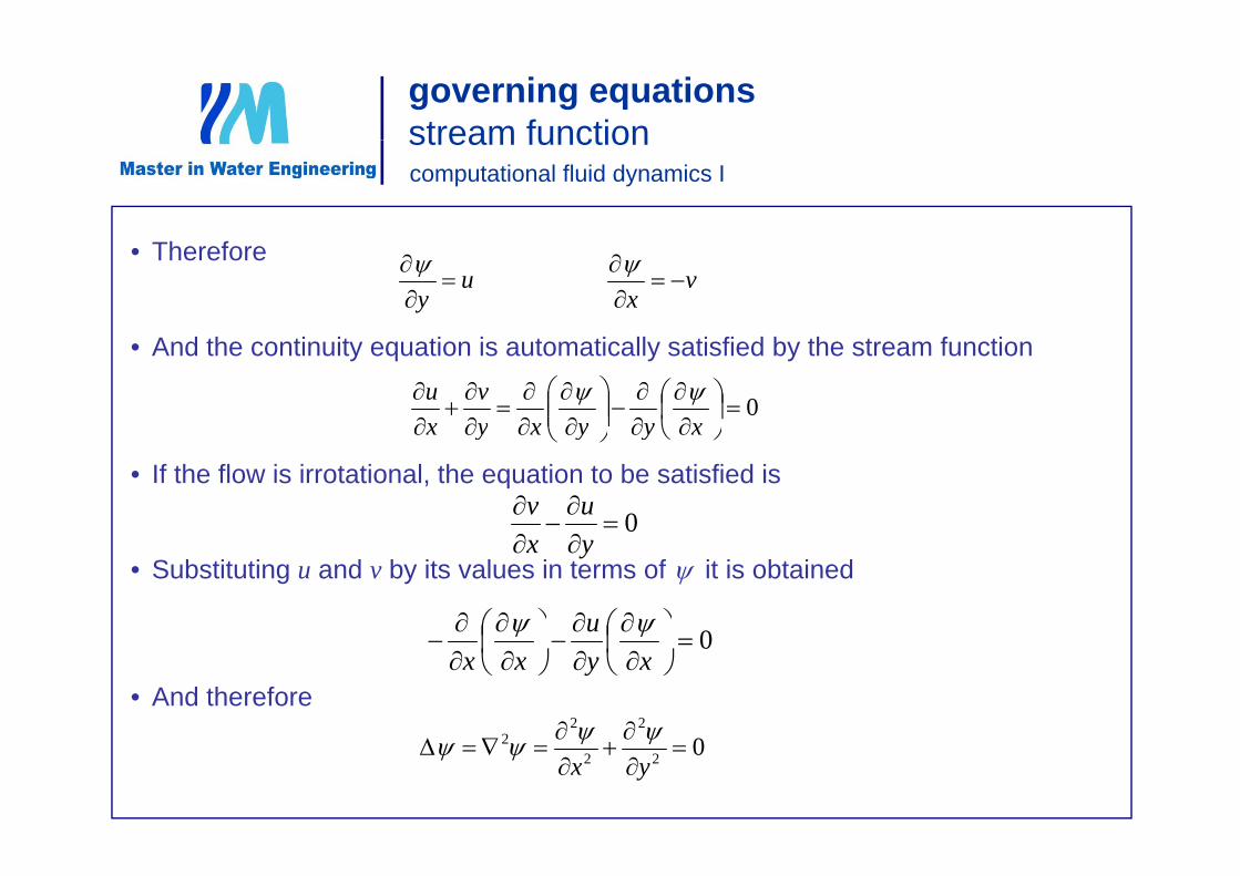
• Therefore

A d th ti it ti i t ti ll ti fi d b th t f ti

uy

v

x

• And the continuity equation is automatically satisfied by the stream function

0

xyyxyv

xu

• If the flow is irrotational, the equation to be satisfied is

yyy

0

uv

• Substituting u and v by its values in terms of it is obtained yx

0

u

• And therefore

0

xyxx

222 0222

yx

governing equationsshallow waters

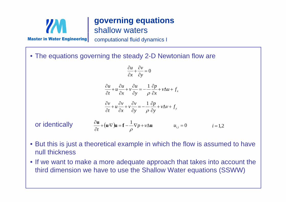
• The equations governing the steady 2 D Newtonian flow are

shallow waterscomputational fluid dynamics I

• The equations governing the steady 2-D Newtonian flow are

0

yv

xu

xfuxp

yuv

xuu

tu

1

or identically

yfvyp

yvv

xvu

tv

1

0 fu

1or identically

• But this is just a theoretical example in which the flow is assumed to have

0, iiu ufuu

pt

· 2,1i

j pnull thickness

• If we want to make a more adequate approach that takes into account the third dimension we have to use the Shallow Water equations (SSWW)third dimension we have to use the Shallow Water equations (SSWW)

Documents

CFD I 1 - caminos.udc.escaminos.udc.es/info/asignaturas/201/CFD I 1.pdfFlow profiles (Curvas de remanso) Non-uniform St d fl Uniform (i=I) St eady flow Rapidly varied flow Broadcrested