From Luttinger liquid to Altshuler-Aronov anomaly in multichannel quantum wires

From Luttinger liquid to Altshuler-Aronov anomaly in multichannel quantum wires

Christophe Mora,1 Reinhold Egger,1 and Alexander Altland2

1Institut für Theoretische Physik, Heinrich-Heine Universität, D-40225 Düsseldorf, Germany2Institut für Theoretische Physik, Universität zu Köln, Zülpicher Str. 77, D-50937 Köln, Germany

�Received 17 February 2006; revised manuscript received 29 May 2006; published 9 January 2007�

A crossover theory connecting Altshuler-Aronov electron-electron interaction corrections and Luttinger liq-uid behavior in quasi-one-dimensional disordered conductors has been formulated. Based on an interactingnonlinear sigma model, we compute the tunneling density of states and the interaction correction to theconductivity, covering the full crossover.

DOI: 10.1103/PhysRevB.75.035310 PACS number�s�: 71.10.Pm, 73.21.�b, 73.63.�b

I. INTRODUCTION

In many regards, the theory of interacting one-dimensional �1D� conductors seems to have reached a maturestate.1,2 In the absence of disorder, interacting 1D conductorsare often described as Luttinger liquids �LL�.1 The LL modelhas been shown to be relevant for a variety of physical sys-tems, e.g., carbon nanotubes, semiconductor quantum wires�QWs�, nanowires, cold atoms in 1D traps, and quantum Halledge states. Thanks to the work of Kane and Fisher,3 a num-ber of precursors,4–6 and a lot of research activity in the pastdecade, the physical properties of both clean LL’s and LL’spolluted by only a few impurities appear to be reasonablywell understood. In particular, various expected scaling lawshave been checked numerically using the functional renor-malization group.7 In the complementary case of signifi-cantly disordered systems, two distinct scenarios may be re-alized: In quantum wires supporting only a small numberN=O�1� of conducting channels, a conspiracy of interactionsand impurity scattering leads to instant localization on mi-croscopic length scales �l, where l is the �renormalized�elastic mean free path. However, in systems with many con-ducting channels—as realized in, for instance, multiwall car-bon nanotubes �MWNTs�—low energy excitations may dif-fuse over distances Nl� l much larger than the mean freepath �before Anderson localization sets in at scales �Nl.�The low-temperature behavior of transport coefficients, tun-neling rates, etc., is governed by strong anomalies differingfrom both the characteristic power laws of the non-Fermiliquid clean LL state, and the strongly localized disorderedfew-channel state. While for thick diffusive wires, both theAltshuler-Aronov corrections to the conductivity8 and thezero-bias anomaly �ZBA� in the tunneling density of states�TDOS� �Refs. 9 and 10� are well understood, much less isknown about the crossover between the LL and the diffusion-dominated regime. In one exemplary study on the TDOS,Mishchenko, Andreev, and Glazman �MAG� �Ref.11� quan-titatively worked out the crossover from a LL dominatedhigh-temperature regime to the diffusive low-energy regime.However, the intermediate physics of several other importantsystem characteristics, say, the conductivity, remains unex-plored.

Motivated by the fact that LL/diffusive crossover sce-narios are realized in several experimentally relevant sys-tems, the purpose of this paper is the construction of a com-

prehensive theory interpolating between the two regimes. Wewill apply this theory to rederive earlier results on the TDOSand to obtain an expression of the conductivity that containsLL power laws and Altshuler-Aronov corrections as limitingcases. Specifically, we will formulate and analyze a model ofspinless electrons with repulsive forward-scattering Coulombinteractions and a short-ranged Gaussian random potential.This model will be shown to reproduce known limiting be-haviors. Of course, in real-life systems, additional mecha-nisms, such as electron-phonon scattering, magnetic impurityscattering, or electronic �e.g., superconducting, charge-density wave, or Peierls� instabilities may also beimportant,12 but we do not address those complications here.The theory of dirty few-channel Luttinger liquids has beenpioneered by Giamarchi and Schulz,13 see also Refs. 14–18for related work. In contrast, we consider here the case ofwide N-channel wires, N�1, termed “quasi-1D” through-out. We note that in the absence of disorder, and despite thepresence of many channels, LL behavior may still berealized.�19� This is well known from studies of many-chainsystems,1,2,12 where an LL phase is observable as long asinterchain hopping can be neglected.20

Besides offering various technical simplifications, themultichannel theory is also of considerable practical interest.For example, MWNTs typically carry N�5 to 20 open chan-nels. Many recent MWNT experiments have shown that theinterplay of disorder and interactions plays a decisive role inthese systems.21–26 On the theoretical side, the TDOS of aMWNT was shown to exhibit a characteristic ZBA at lowenergies.11,27,28 As far as we know, no results for the interac-tion correction to the Drude conductivity for arbitrary disor-der have been published so far. Other examples of experi-mental interest include quasi-1D organic conductors,29

charge-density wave nanowires,30 polymer nanofibers,31

In2O3 wires,32 or MoSe nanowires.33 In particular, InAsnanowires currently receive a great deal of attention. Theyhave typical mean free paths of the order of 10 to 100 nm,with N�10 to several 100 and lengths of microns up tomillimeters.

Both LL power laws and the low-temperature anomaliesin diffusive systems root in the same physical mechanism:Scattering off impurities creates a 2kF oscillatory screeningcloud �Friedel oscillation� in the conduction electron densitywhich acts as an additional source of backscattering. Thisidea was put forward in Ref. 34 for a weakly interacting 1Dsystem with a single barrier. For a disordered two-

PHYSICAL REVIEW B 75, 035310 �2007�

1098-0121/2007/75�3�/035310�14� ©2007 The American Physical Society035310-1

http://dx.doi.org/10.1103/PhysRevB.75.035310

dimensional system, the ZBA �Ref. 35� and theconductivity36,37 were explored for arbitrary T�0 within aperturbative diagrammatic framework. However, in �quasi�1D, the power-law decay exponent of the Friedel oscillationitself is affected by interactions, and the simple picture out-lined above no longer applies. Relatedly, Fermi liquid renor-malization procedures36 must break down in the 1D setting.1

A coherent description of quasi-1D systems rather requiresthe construction of a generalized approach, and will be themain subject of this paper. We note in passing that recentwork by Golubev et al.39,40 has also explored similar cross-over phenomena in granular models.

Building on a replicated coherent-state field integral, wewill derive an interacting nonlinear � model �NL�M�, simi-lar in spirit to that of Ref. 38. This field theory will allow fora nonperturbative treatment of interaction diagrams thatdominate in the ballistic limit and thereby capture the rel-evant LL physics without invoking standard bosonizationschemes.41 A superimposed perturbative treatment will thenallow us to compute the low-temperature diffusive correc-tions to the conductivity in conceptual analogy to earlier dia-grammatic approaches. �In many respects, the ideas enteringthis combination of perturbative and nonperturbative ele-ments are similar to those developed in the theory of Kame-nev and Andreev.9�

The rest of the paper is organized as follows. In Sec. II,we describe the model and the field-theoretical approachtaken here. The TDOS is discussed in Sec. III, while thelinear conductivity will be studied in Sec. IV. Finally, in Sec.V, we conclude and offer an outlook. Technical details havebeen delegated to several Appendixes. Below, we set �=kB=1.

II. MODEL AND FIELD-THEORETICAL APPROACH

A. Model

We consider a disordered and interacting quasi-1D quan-tum wire supporting N conducting channels below the Fermienergy. To describe the system we employ the prototypicalHamiltonian

H = H0 + Hdis + HI, �1�

where

H0 = − i�C

vFC� dx �†�x� ,

represents the kinetic energy, C= ±1 labels right- and left-moving states, vF is the Fermi velocity, and �= ��1,C , . . . ,�N,C� is an N-component vector of field opera-tors. Disorder scattering is described by

Hdis = HFS + HBS, �2�

HFS = �C� dx �C

† �x�VC�x��C�x� , �3�

HBS =� dx �R†�x�W�x��L�x� + H.c., �4�

where HFS and HBS represent the forward �FS� and the back-

ward �BS� scattering, respectively. Here, VC= Vnn��x� and

W= Wnn��x� are N�N matrices in channel space which weassume to be randomly distributed. Specifically,

�Wnm�x�Wm�n�* �x��dis =

1

2��1�0nn�mm��x − x�� , �5�

where �1=N /�vF is the 1D density of states and �0 the �bare�elastic scattering time. The �bare� mean free path then is l=vF�0. Finally, defining the local electron density as =�CC, C=�C

† �C, the interaction Hamiltonian is defined as

HI =U

2� dx 2�x� , �6�

where the constant U sets the interaction strength. TheHamiltonian implies several idealizing assumptions: Linear-izable spectrum, channel-independent Fermi velocity, ab-sence of electron-electron backscattering, and a number ofothers more. In Appendix A we detail how the above Hamil-tonian may be derived from a more microscopic model, e.g.,one describing a MWNT. In particular, we will argue that atenergies �� smaller than the characteristic energy abovewhich structures in the direction transverse to the wire areresolved, the above model Hamiltonian properly describesall relevant system characteristics.

Following and generalizing Ref. 13, a further simplifica-tion may be effected by a gauge transformation removing theforward scattering disorder. For N=1, forward scatteringmerely leads to phase multiplying the electron wave func-tions and, therefore, does not affect �gauge invariant� observ-ables. A non-Abelian generalization of that argument may be

used to eliminate the forward scattering matrices Vc. To thisend, we perform the unitary transformation �C�x�=UC�x��C�x�, where

UC�x� = P exp − iC

vF�x

dx�VC�x�� 7�

with the path-ordering operator P defined via

P exp −iC

vF�x

dx�V�x�� n=0

�− iC/vF�n

� �x

dxn�xn

dxn−1 ¯ �x2

dx1

� V�xn�V�xn−1� ¯ V�x1� .

This unitary transformation eliminates all FS processes, H0+HFS→H0, when H is expressed in terms of the “new” fer-

mions, �C. One can check explicitly that under this unitary

transformation, HBS does not change its structure, and W�x�remains a Gaussian random variable with statistical proper-ties �5�. Moreover, the gauge invariant interaction term HIand all observables studied below remain unaffected by this

MORA, EGGER, AND ALTLAND PHYSICAL REVIEW B 75, 035310 �2007�

035310-2

transformation.42 From now on, we switch to the fields �and rename them �. Effectively, we can then forget aboutthe FS processes.

Before proceeding we note that the clean HamiltonianH0+HI describes a �multichannel� LL phase, described bythe dimensionless Luttinger interaction parameter K and theplasmon velocity v,

K =1

�1 + �1U, v = vF/K . �8�

This LL phase comes along with N−1 �effectively noninter-acting� plasmon excitations moving at velocity vF.19 For K=1, we retrieve a Fermi gas, while the repulsively interactingcase corresponds to K�1.

B. Hubbard-Stratonovich transformations

Our aim is to formulate a tractable low-energy field theoryfrom the above model. Restricting ourselves to equilibriumphenomena, we will employ an imaginary time formalismand the replica trick: To compute the free energy F=−T ln Z, we use ln Z=limr→0�Zr−1� /r and represent the dis-order average of the rth power of the partition function�Zr�dis in terms of an r-fold replicated coherent-state Grass-mann field �nC��x ,��, where �=1, . . . ,r. �As usual, an ana-lytic continuation r→0 to be performed in the end of thecalculation is implied.�

We begin by decoupling the interaction Hamiltonian in astandard way via a Hubbard-Stratonovich �HS� transforma-tion. Introducing the �replicated� real field ��x ,��, this gen-erates the action for the interaction part,

SI = �� dx d��

2

2U+ i�� . �9�

Note that the fields � do not carry a channel index, butcouple only to the 1D density �x�. �For the more generalcase g2�g4 discussed in Appendix A one introduces a dou-blet �C and proceeds in a similar way.�

One advantage of the replicated framework is that thedisorder average may be conveniently performed at an earlystage of the calculation. The action describing the disordercontribution to �Zr�dis then assumes the form

Sdis =1

4��1�0�

C,nm,�� dx d� d�� nC��x,��nC��x,��

� �m,−C,��x,��m,−C,��x,�� ,

where we used Eq. �5�. We decouple the time-nonlocal actionSdis by another Hubbard-Stratonovich transformation to ob-tain

Sdis =��1

8�0� dx d� d��

��

QR,��x,�,��QL,��x,��,��

+i

4�0� dx d� d��

nC,��

��nC��x,��QC,��x,�,��nC��x,�� . �10�

This HS transformation introduces a functional integral overa pair of time-bilocal but spatially local auxiliary matrix

fields QR/L. To warrant convergence of the functional inte-gral, the condition

QR† = QL �11�

is imposed. Implicitly understood in the above discussion isthe case of broken time-reversal invariance, e.g., by applica-tion of a weak magnetic field. Otherwise, proper inclusion ofthe Cooperon channel �describing, e.g., one-loop weak local-ization effects� would require an additional doubling of thefield degrees of freedom.38

At this stage, we may integrate out the fermion fields toarrive at the action

S�Q,�� =1

2Tr�U−1� +

��1

8�0Tr�QRQL�

− N�C=±

Tr ln��C + i� +i

4�0QC� , �12�

where �C=��− iCvF�x. The trace symbol indicates summa-tion over replica indices and integration over space and�imaginary� time.

In the noninteracting limit U=0, a standard gradient ex-pansion of the tracelog in Eq. �12� leads to a diffusive action.This expansion is stabilized by the condition N�1 �for N=1, there is of course no diffusive phase�, and starts by iden-tifying the saddle-point solution. It is convenient to switchfrom time to energy space via a double Fourier transform.The saddle configurations are then homogeneous �x indepen-

dent�, parity invariant �QR= QL�, and time-translational in-variant �diagonal in energy space�. The noninteracting saddle

QR/L=� can be expressed using the standard notation38

��,�� = sgn��. �13�

�Our Fourier convention is ��x ,��=T �� dq /2��eiqx+i��q ,��, with fermionic Matsubarafrequencies �= �2m+1��T �integer m�.� In order to study dif-fusion properties, we need to include fluctuation modesaround the saddle �. There is one important subtlety at thatstage, which we discuss in detail in Appendix B; namely,there are two different types of massive fluctuation modes.

These are �i� excitations with Q2�1 and �ii� chirally asym-

metric excitations with Q2=1 but QL� QR �involving thefield W1 in Sec. II E�. Excitations of type �i� are not coupledto massless fluctuations at the Gaussian level, and hence cansafely be neglected. However, type-�ii� excitations are lin-early coupled to massless excitations �the field W0 in Sec.

FROM LUTTINGER LIQUID TO ALTSHULER-ARONOV… PHYSICAL REVIEW B 75, 035310 �2007�

035310-3

II E�, and thus cannot simply be ignored. In fact, only whenintegrating them out, do we obtain the physically meaningful1D result for the longitudinal diffusion constant, D=vF

2�0.Moreover, we also recover the transversal diffusion constant.Including only Gaussian fluctuations around the saddle �13�,we thus reproduce the full anisotropic �cf. remark at the endof Appendix B� diffusive theory,11,27 with the correct longi-tudinal and transversal diffusion constants. This provides ana posteriori justification of the simplifying assumptions un-derlying the effective Hamiltonian �1�.

C. Chiral anomaly

We now turn to the interacting case and look for thesaddle-point configurations corresponding to the action �12�.Unfortunately, we are unable to determine the exact saddle,except for the clean limit ��0→ �. Hence we will adopt anansatz, motivated by Ref. 9, which will lead to results gen-erally exact to lowest order in U, and to any order in theballistic limit. �In the diffusive case, the approximate saddlepoint scheme is good enough to address the strongest low-temperature singularities in transport coefficients.� Specifi-cally, we will, for fixed ��, consider field configurations ofthe form

QC�x,�,�� = eiKC�x,�� − ��e−iKC�x,��, �14�

i.e., configurations differing from the noninteracting saddle

QC=� only by a chiral gauge transformation, mediated by aspace-time local field KC= KC��x ,��. Varying the actionwith respect to KC determines the particular KC that solvesthe saddle-point equation to lowest order in the interaction.

Before proceeding to the saddle-point solution, let us ana-lyze the effect of a gauge transformation breaking chiralsymmetry. To remove the phase factors dressing � in Eq.�14�, we apply a gauge transformation to the fermionic fieldscorresponding to the tracelog in Eq. �12�,

�C�x,�� eiKC�x,��C�x,�� . �15�

This transformation has two effects, namely �i� the term � inthe tracelog is replaced by �C, where

�C = � + �CKC, �16�

and �ii� the classical chiral U�1� invariance is broken at thequantum level, leading to a chiral anomaly.43,44 The anomalyarises from the Jacobian of the measure of the fermionic pathintegral under the chiral gauge transformation �15�, and is atthe basis of path-integral bosonization. The calculation canbe done by separating gauge transformations like Eq. �15�into infinitesimal steps, and then adding the correspondingJacobian contributions.44 One finds that the QC fields, de-scribing low-energy properties, do not contribute to theanomaly �which is a high-energy feature�. For the sake ofsimplicity, however, we show here a different derivationsolely relying on known results for the clean case.

We first recapitulate the “standard” form of the anomaly,43

− N Tr ln��C + i�� = − N Tr ln��C� +1

2Tr��C�� , �17�

where the frequency-momentum representation of the chiralpolarization bubble is given by

�C�q,�m� =�1

2

vFq

vFq + iC�m�18�

and �m=2�mT �integer m� are bosonic Matsubara frequen-cies. For later convenience, we also define

��q,�m� = �C

�C�q,�m� = �1�vFq�2

�vFq�2 + �m2 . �19�

We then use the identity

Tr ln��C + i� +i

4�0QC� = Tr ln��C + i��

+ Tr ln�1 +i

4�0��C + i��−1QC�

= Tr ln��C + i��

+ Tr ln�1 +i

4�0��C + i�C�−1�� ,

�20�

where QC is given by Eq. �14�, and we used

e−iKC��C + i��−1eiKC = ��C + i�C�−1

and the cyclic invariance of the trace. �Unlike with the UVsingular logarithmic contribution to the trace, usage of “cy-clic invariance” is a permissible operation in the expansionterms.� Similarly,

Tr ln��C + i�C +i

4�0�� = Tr ln��C + i�C�

+ Tr ln�1 +i

4�0��C + i�C�−1�� .

�21�

Subtracting Eqs. �20� and �21�, and using Eq. �17�, we obtain

− N Tr ln��C + i� +i

4�0eiKC�e−iKC�

= − N Tr ln��C + i�C +i

4�0��

+1

2Tr��C�� −

1

2Tr��C�C�C� . �22�

The last two terms constitute the chiral anomaly contributionto the action. Summing over C, the anomaly reads Sa

= 12 Tr��a��, with


035310-4

�a = � − �C

�C

��C

�C

�. �23�

Clearly, both �C and �a depend on the field KC. As a result,Eq. �14� together with the gauge transformation �15� puts theaction �12� into the equivalent form

S = 12 Tr��U−1 + �a�� +

��1

8�0Tr�eiK2�e−iK2��

− N�C


4�0�� , �24�

where K2=KR−KL.

D. Saddle-point solution

Our so far discussion applied to arbitrary time-dependentgauge transformations KC. We now wish to find values of KCsuch that the transformed Q field �14� represents an �approxi-mate� saddle point of the theory. To this end, we define

QC = eiKCQCe−iKC �25�

and determine KC such that at QC=� the action is approxi-mately stationary. Put differently, we require that at thesaddle-point values of KC, first-order variations QC→�+QC vanish. Substituting �→�+QC into Eq. �24� andexpanding to linear order in QC, we thus obtain the saddle-point equations �one for each value of C=±�

e−iCK2�x,�� − ��eiCK2�x,�� =2iN

��1��C + i�C +

i

4�0��

x,�,��

−1

.

�26�

These equations can generally not be solved exactly. Follow-ing Ref. 9 we will thus be content with determining a solu-tion that holds to leading order in the interaction strength U.Expanding Eq. �26� to lowest order in � and hence U, wefind

�K2,��− =2iNC

��1�GC�� + �CKC�GC�x,�,��. �27�

Here we define the noninteracting chiral disordered Greenfunction as�45�

GC−1 = �C + �i/4�0�� . �28�

One may then check that

KC��q,�m� =i�m + qvFC + i sgn��m�/�0

�m2 + �qvF�2 + ��m�/�0

��q,�m� �29�

solves Eq. �27�. In the clean �ballistic� limit, the solutionreduces to

KC�q,�m� = −��q,�m�

i�m − CvFq.

Indeed, these functions represent exact �to all orders in U�solutions of the saddle point equation �26�. In the comple-mentary diffusive limit ��m ��0 , �q � l�1, KR/L asymptote to9

KR/L�q,�m� =i sgn��m�Dq2 + ��m�

��q,�m� ,

where D=vF2�0 and the left-right asymmetry vanishes. With

Eq. �29�, �C follows from Eq. �16� as

�C�q,�� = 2vFqvFq + iC�� + sgn��/2�0�

�2 + �vFq�2 + ��/�0��q,�� , �30�

and Eq. �23� yields

�a�q,�� = �1�vFq�2− 3�vFq�2 + �� + 1/�0�2

��2 + �vFq�2 + ��/�0�2 . �31�

E. Interacting nonlinear sigma model

Let us now substitute Eq. �25� into the original action �12�to obtain

S =1

2Tr��U−1 + �a�� +

��1

8�0Tr�eiK2QRe−iK2QL�

− N�C=±


4�0QC� . �32�

To make further progress, we need to include fluctuations inQC around the saddle � of the interacting system. Thesefluctuations may be conveniently parametrized as

QC = TC�TC−1, TC = exp�− W0/2�exp�iCW1/2� , �33�

where �W0,1 ,��+=0 for the relevant low-energy modes.�Fluctuations departing from the manifold �33� are massiveand decoupled from massless excitations at the Gaussianlevel. Therefore they have no significant effect as long asN�1.� The condition �W0,1 ,��+=0 is resolved by setting

W0,1 = � 0 B0,1

− B0,1† 0

� , �34�

where the 2�2 structure refers to energy space ��0,��0�. The soft fluctuations of the theory are thus param-etrized by unconstrained complex-valued matrix elements�B0,1��,��x�, with ��0,��0. Note that this parametriza-tion gives QR

† =QL as required by Eq. �11�, and QR2 =QL

2 =1.At this point, it is convenient to integrate out high-energy

fluctuations of the field � within the framework of a standardrenormalization group �RG� analysis.13 Starting with thebandwidth �c �which is of the order of the Fermi energy� asan UV cutoff, we subsequently integrate out all � fields inthe strip �c�� m � ��c. Here the intermediate cutoff�c�� 0

−1 ,T�, but small enough to allow for a perturbativetreatment of the remaining �low-energy� interaction field. Wewill show in Sec. IV A that the precise value of �c� drops outin the calculation of observables like the interaction correc-tion to the conductivity. To implement the RG, we tempo-rarily switch to yet another gauge representation of thetheory, viz.


035310-5

S =1

2Tr��U−1 + �� +

��1

8�0Tr�eiK2QRe−iK2QL�

− N�C

Tr ln��C +i

4�0ei�KC−KC

0 �QCe−i�KC−KC0 �� , �35�

differing from Eq. �32� by a gauge transformation mediatedby exp(i�KC

0 −KC�), where �CKC0 =−�. Within the high-energy

strip, B fluctuations, coupling to the action through a “low-energy” perturbation of O�1/�0�, are expected to be of noimportance, and will be disregarded here. It then turns outthat high-energy � fluctuations renormalize both �0’s, the onein the second term and that inside the tracelog of Eq. �35�, inthe same manner. Since KC−KC

0 =K2 for high energies, thisrenormalization follows by evaluation of �ei�K2�x,��−K2�x,0�� forenergies within the strip, using the first term of Eq. �35� tocarry out this Gaussian average. As a net result, we end upwith an effective renormalization of the mean free time,

�0 → �0� = �0��c�/�c��i, �36�

with the Luttinger liquid power-law exponent for weak back-scattering by a single impurity,3

�i = 2�1 − K�/N , �37�

where K is the Luttinger parameter �8�. In what follows, weimagine that the RG has been carried out, and only discussits effects explicitly where required. �In Sec. III, it will infact be more convenient not to perform the RG transforma-tion at all.�

Its logarithmic nonlinearity makes the general analysis ofthe action �32� difficult. For momenta q�1/ �vF�0��, and fre-quencies ��0�

−1, probing the multiple scattering regime, agradient expansion in small momenta can be performed toobtain

S =1

2Tr��U−1 + �a�� +

��1

8�0Tr�TR�TR

−1e−iK2TL�TL−1eiK2�

+i��1

2 �C

Tr„��TC−1�CTC + i�C�…

+��1vF

2 �C

Tr„GC�TC−1�CTC + i�C�…2 + ¯ , �38�

where the Green functions are given by Eq. �28�. In Appen-dix B we show how the standard form of the diffusive �model may be obtained from this prototype action. However,for arbitrary momenta and frequencies no such reduction ispossible. Nonetheless progress can be made, viz. by notingthat an expansion of the action �32� to second order in thefluctuation generators B is sufficient to compute our observ-ables of prime interest. In essence, this expansion is tanta-mount to a random-phase approximation �RPA� approxima-tion to the model where the “RPA bubble” accounts forimpurity scattering. Our neglect of higher-order fluctuationsessentially implies that the renormalization of diffusion andinteraction by quantum interference processes is not takeninto account.

III. ZERO-BIAS ANOMALY

To warm up, before addressing the more involved inter-action corrections to the conductivity in Sec. IV, let us brieflydiscuss the energy-dependent bulk tunneling density of states�TDOS�; see also Refs. 11, 27, and 28. The TDOS governstemperature- or voltage-dependent transport quantities whencontacts or other conductors are weakly coupled to the QW.It is well known that in both limits, Luttinger and diffusive,the DOS exhibits pronounced structure as a function of en-ergy. The crossover between the two limiting scenarios wasaddressed by MAG �Ref. 11� by a direct analysis of thescreened interaction in multichannel quantum wires. We hererederive and extend their results, essentially to illustrate theapplication of the present formalism.

For a particle-hole symmetric system, the TDOS is1

��,T� = − �2/��coth��/2T��C�

0

dt sin �t Im GC�t� ,

�39�

where GC�t� is the real time analytic continuation, �→ it+0+, of

�n

�T��nC�x,��nC�x,0�� = − i��1��ei�KC�x,��−KC�x,0��S�,

�40�

T� the time-ordering operator, and x an �arbitrary� space co-ordinate. Since GR=GL, we are free to focus on GR. In Eq.�40�, fluctuations TC�1 do not contribute, and the average inEq. �40� is taken using the action S� obtained from Eq. �32�with TC=1. �The replica limit is then trivial to take.� Fornoninteracting fermions, KC=0, and hence

GR�t� = − i��1��t� = − i��1T/sinh��Tt� ,

��,T� = 2�1T coth��/2T��0

dtsin��t�

sinh��Tt�= �1.

In order to analytically evaluate �ei�KR�x,��−KR�x,0��S�, we ex-

pand S� to quadratic order in �, leading to

S� =1

2Tr ��0� . �41�

This truncation does not introduce any approximation in theballistic limit and is consistent with the weak-interactioncondition inherent in the construction of the saddle �14�. Thekernel �0 includes �i� the term �U−1+�a�, �ii� a contributionfrom the second term in Eq. �32�, and �iii� a term�Tr�GC�C�2 from the expansion of the tracelog. For in-stance, �ii� gives

��1

8�0Tr��K2�K2 − K2

2� = Tr��− q,− ��

��1�vFq�2��/2�0

��2 + �vFq�2 + ��/�0�2��q,�� .

Combining all three terms, the kernel in Eq. �41� reads


035310-6

�0�q,�m� =1

U+ �1

�vFq�2

�m2 + �vFq�2 + ��m�/�0

. �42�

This expression bridges the ballistic and diffusive regimes. Itis exact in the LL limit, while it describes diffusivelyscreened interactions in the opposite limit, assuming weakinteractions.

It is then straightforward to arrive at the TDOS. With thedefinition �8� of the LL parameter K, and the bulk �� andboundary ��b� Luttinger tunneling exponents,19

� = �K + 1/K − 2�/2N, �b = �1/K − 1�/N , �43�

some algebra leads to46

��,T��1

=2

�coth��/2T�Re�

0

dt

tsin��t�

� � �Tt

sinh��Tt��+1

�1 + i�ct�−�

� e�F1�t/�0,T�+�bH1�t/�0,T�+i�F2�t/�0�+i�bH2�t/�0�,

�44�

where we have defined

F1�y,T� = Re�0

du�1

u−

1�u2 + iu

� 1 − cos�2yu�tanh„u/�2T�0�…

,

F2�y� =�

2�1 − I0�y�e−y� ,

H1�y,T� =Im

2�

0

duu + i

�u2 + iu�3/2

1 − cos�2yu�tanh„u/�2T�0�…

,

H2�y� = −�

2ye−y�I1�y� + I0�y�� ,

and I0,1 are Bessel functions of imaginary argument.47 ForT=0, the integrals for F1 and H1 can be evaluated in closedform,

F1�y,0� = − ln�2e−C

y� + K0�y�cosh�y� ,

H1�y,0� = 1 − y�cosh�y�K1�y� + sinh�y�K0�y�� ,

where C=0.577. . . is the Euler constant, and K0,1 are relatedBessel functions of imaginary argument.47 Note again thatEq. �44� has been derived under the assumption of largechannel number N.

Before proceeding, let us pause to briefly comment on therelation of Eq. �44� to the results of MAG. The far reachingequivalence between Eq. �44� and MAG’s Eq. �14� is bestexposed by shifting their integration variable t according tot→ t− i /2T. The results then turn out to be identical, pro-vided one identifies the integral kernel V�� of MAG with

V�� = −1/K − 1

2NRe

��1 − K� + i/�0

�3/2�� + i/�0

.

Effectively, however, in MAG the limiting case of stronginteractions and/or large channel number, K→0, is consid-ered. In the ballistic regime, and for moderate interactionsand channel numbers, their results do, therefore, not scaleaccording to the Luttinger exponent Eq. �43�. Within theframework of MAG’s analysis, this deviation is howeverstraightforward to avoid by not taking the limit of stronginteractions at an early stage.

We next discuss Eq. �44� in various limits of interest.Beginning with the zero temperature case, T=0, for ��0�1,only small t contribute to the integral �44�. The functions F1,2and H1,2 are then basically negligible, the t integral can bedone, and we obtain the well-known LL power-law TDOS,1

��1

=1

��1 + ��/�c�� 45�

with the gamma function ��x�. In the diffusive regime,��0�1, large t dominate in Eq. �44�, and one can useasymptotic expansions for F1,2 and H1,2. Actually, the precisecrossover scale separating the diffusive from the ballistic re-gime in the T=0 TDOS is set by ��0��; see Ref. 11. Withthe error function �, we find

��1

=eC�+�b

�2�c�0�� 1 − �� 2�

��0�b��

�eC�+�b

�2�c�0��

��0/2

��be−2��b

2/��0�, �46�

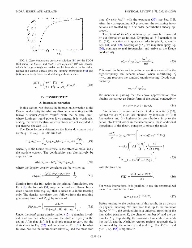
corresponding to an exponentially vanishing TDOS at lowenergies. This pseudogap behavior was first noted byNazarov,10 and subsequently rederived in Refs. 11 and 28.While a direct expansion of the sin��t� in Eq. �44� wouldsuggest a linearly vanishing TDOS,28 the correct result is thenonperturbative exponential law �46�. In fact, one can showby complex integration methods that in the 1D case the pref-actor of any polynomial-in-� term must vanish. Similarly,one can show that the T dependence of ��=0� also has tobe exponential as T→0. Figure 1 shows the full T=0 cross-over solution together with the asymptotic results �45� and�46�.

Next we turn to the regime T�0�1 and ��0�1. Thecrossover function describing the transition from ��T to��T, reported in Ref. 11, can be reproduced from Eq. �44�using asympotic expansions of F1,2 and H1,2. In particular,for ��T�1/�0,

�T��1

=eC�+�b

�2�c�0��

2.389� T�0

2��b2�1/4

e−1.075�b�2�/T�0.

�47�

Finally, once either T�0�1 or ��0�1, typical values fort in Eq. �44� are t�min�1/T ,1 /��, such that effectively thestandard LL power laws are recovered. For T� �1/�0 ,��,


035310-7

�T��1

� ��

2�� 1 + ��

�2�1 + �/2��T/�c��. �48�

IV. CONDUCTIVITY

A. Interaction correction

In this section, we discuss the interaction correction to theDrude conductivity for arbitrary disorder, connecting the dif-fusive Altshuler-Aronov result�8� with the ballistic limit,where Luttinger liquid power laws emerge. It is worth reit-erating that weak localization corrections are not included inour theory; see Sec. II B.

The Kubo formula determines the linear dc conductivityas the q→0, i�m→�+ i0+ limit of

��q,�m� = −e2

�m�j�q,�m�j�− q,− �m�� +

e20

m�m, �49�

where 0 is the Drude resistivity, m the effective mass, and jthe particle current. The conductivity can alternatively beexpressed as

��q,�m� = − �e/q�2�mP�q,�m� , �50�

where the density-density correlator can be written as

P�q,�� =��q,��− q,− ��

U2 −1

U. �51�

Starting from the full action in the original formulation, seeEq. �12�, the formula �51� may be derived as follows: Intro-duce a source field ��q ,�m� that is added to � in the tracelogonly. The density correlator then follows from the resultinggenerating functional Z�� by means of

P�q,�m� = � �2 ln Z

��q,�m� � ��− q,− �m��=0. �52�

Under the local gauge transformation �15�, � remains invari-ant, and one can safely perform the shift �→�−� in theaction. After that shift, it is a simple matter to carry out thederivatives in Eq. �52� and to arrive at Eq. �51�. In whatfollows, we use the intermediate cutoff �c� and the mean free

time �0�=�0��c� /�c��i with the exponent �37�; see Sec. II E.After the corresponding RG procedure, the remaining inter-actions are treated by a first-order perturbation theory ap-proach.

The classical Drude conductivity can now be recoveredby our formalism as follows. Dropping all B fluctuations inEq. �38�, the action up to quadratic order in � is S�, given byEqs. �41� and �42�. Keeping only S�, we may then apply Eq.�50�, continue to real frequencies, and arrive at the Drudeconductivity

�D� = e2�1vF2�0� =

Ne2vF

��0�. �53�

This result includes an interaction correction encoded in thehigh-frequency RG scheme above. When substituting �0�→�0, one recovers the standard �noninteracting� Drude con-ductivity,

�D = e2�1vF2�0.

We mention in passing that the above approximation alsoobtains the correct ac Drude form of the optical conductivity

�D�� = �D/�1 − i��0� . �54�

Interaction corrections to the dc Drude conductivity �53�,defined via �=�D� +��, are obtained by inclusion of �i� Bfluctuations and �ii� higher-order contributions in � to theaction. To lowest order in the interactions, these additionalingredients to the theory conspire to obtain the result

��T��D

= ��c�0�−�i/�1+�i� 1 + �iln�2�e−1−CT�0��

− �iRe�0

d�F��

��

� + i/�0�− 1

+i

2�0��1 + K��2 + i�/�0�� , �55�

with the function

F�� =�� coth��/2T��

��. �56�

For weak interactions, it is justified to use the renormalizedmean free time in the form

�0� = �0��c�0�−�i/��i+1�. �57�

Before turning to the derivation of this result, let us discussits physical meaning. We first note that, up to the prefactor��c�0�−�i/��i+1�, the conductivity is a universal function of theinteraction parameter K, the channel number N, and the pa-rameter T�0�. Importantly, the crossover temperature separat-ing the LL and the Altshuler-Aronov regions, respectively, isdetermined by the renormalized scale �0�. For T�0��1 and��1, Eq. �55� simplifies to

FIG. 1. Zero-temperature crossover solution �44� for the TDOS�full curve� at K=0.3 and N=5. Here �c�0=5�104 was chosen,which is large enough to render results insensitive to its value.Dotted and dashed curves give the limiting expressions �46� and�45�, respectively. Note the double-logarithmic scales.


035310-8

��T��D

� ��c�0��−�i�1 + �iln�2�e−�1+C�T�0��, T � ��−1.

�58�

Exponentiation of the logarithm obtains the familiar Lut-tinger liquid high-temperature power law,4,13,18

��T��D

� e−�i�1+C��2�T/�c��i, T � ��−1, �59�

otherwise obtained by stopping the RG procedure of Sec.II E at T��−1. Governed by the single-impurity back-scattering exponent �i �cf. Eq. �37� and Ref. 3�, the exponen-tiated form is valid only at asymptotically large temperatureswhere multiple interference is negligible. In the complemen-tary regime T�0��1 the interaction correction becomes

� − �D

�D� − �i

3��/2��− 1/2�1 + K

�T�0��−1/2, �60�

where � is the Riemann zeta function.47 This expression re-covers the well-known T−1/2 Altshuler-Aronov correction in1D,8 leading to a pronounced suppression of the conductivityat low temperatures. At very low temperatures, this correc-tion becomes sizeable and our first-order perturbative ap-proach ceases to be valid. In that case, also quantum inter-ference corrections have to be included.

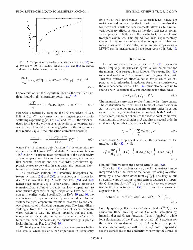
The crossover solution �55� smoothly interpolates be-tween the limits �59� and �60�, respectively, as is shown forK=0.9 and N=30 in Fig. 2. Note that Eqs. �59� and �60�match each other at T�0� of order unity. Related crossoverscenarios from diffusive dynamics at low temperatures tonondiffusive dynamics at high temperature have been dis-cussed in earlier work. Specifically, in Refs. 39 and 40, theconductance of a quantum dot array was considered. In thatsystem the high-temperature regime is governed by the cha-otic dynamics of individual quantum dots. The latter differsstrikingly from the ballistic dynamics of clean quantumwires which is why the results obtained for the high-temperature conductivity corrections are quantitatively dif-ferent from ours. �Nonetheless, the qualitative high-T profilelooks similar; cf. Fig. 2 of Ref. 39.�

We finally note that our calculation above ignores finite-size effects, which are of minor importance in sufficiently

long wires with good contact to external leads, where theresistance is dominated by the intrinsic part. Note also thatfour-terminal resistance measurements allow us to circum-vent boundary effects as long as the electrodes act as nonin-vasive probes. In both cases, the conductivity is the relevanttransport coefficient. This regime has been experimentallystudied in carbon nanotubes and other quantum wires formany years now. In particular, linear voltage drops along aMWNT can be measured and have been reported in Ref. 48.

B. Derivation

Let us now sketch the derivation of Eq. �55�. For nota-tional simplicity, the primes in �0� and �c� will be omitted forthe moment. Our strategy is as follows: We expand Eq. �32�to second order in B fluctuations, and integrate them out.This will generate an effective action for �, which we ex-pand up to fourth order. In addition, for internal consistency,the B-independent terms in Eq. �32� must also be kept up tofourth order. Schematically, our starting action then reads

S = S� + SB + S4�1� + S4

�2�. �61�

The interaction correction results from the last three terms.The contribution SB combines �i� terms of second order inB0,1 but zeroth order in �, and �ii� of first order in B butsecond order in �. Note that the first order in both B and � isstrictly zero, due to our choice of the saddle point. Moreover,contributions to second order in B and first or second order in� identically vanish in the replica limit. Finally,

S4�1� =

��1vF

4 �C

Tr�GC�C�4 �62�

comes from B-independent terms in the expansion of thetracelog in Eq. �32�, while

S4�2� =

��1

8�0� 1

12Tr K2

4 −1

3Tr �K2�K2

3 +1

4Tr �K2

2�K22��63�

similarly follows from the second term in Eq. �32�.Since Eq. �51� involves only �, the B fluctuations can be

integrated out at the level of the action, replacing SB effec-tively by a new fourth-order term S4

�3��. The lengthy butstraightforward derivation of this term is detailed in Appen-dix C. Defining S4�S4

�1�+S4�2�+S4

�3�, the lowest-order correc-tion to the conductivity, Eq. �51�, is obtained by first-orderexpansion in S4,

P�q,�� = − U−2��q,��− q,− ��S4 − �S4�S��S�

.

�64�

Loosely speaking, fluctuations of the � field �S4�1� ,S4

�2�� de-scribe the RPA screening of the Coulomb interaction byimpurity-dressed Green functions �“empty bubble”�, whilejoint fluctuations of the B and the � field �S4

�3�� account forthe vertex renormalization of the RPA bubbles by impurityladders. Accordingly, we will find that S4

�3� holds responsiblefor the corrections to the conductivity showing the strongest

FIG. 2. Temperature dependence of the conductivity �55� forK=0.9 and N=30. The limiting behaviors �59� and �60� are shownas dotted and dashed curves, respectively.


035310-9

low-temperature singularities. Conversely, the terms S4�1� ,S4

�2�

dominantly contribute to the conductivity in the Luttingerlimit T�0��1.

Doing the � contractions, we obtain for the conductivity

� = − �D Im� d�

�F�� dq

2��0,R

−1 �q,��

� �vFq�2 �K1 + K2 + K3��q,��vF

2q2 − �2 − i�/�0�2 , �65�

with the auxiliary quantities

K1�q,�� = 4�1 +1 − 2i��0

�2vFq�0�2 + �1 − 2i�0�0�2� ,

K2�q,�� = − 2,

K3�q,�� =1

�02�vF

2q2 − �2 − i�/�0�

�2 − 6i��0 − �2��0�2 + �2vFq�0�2

�1 − 2i��0�2 + �2vFq�0�2 , �66�

where the function F�� has been defined in Eq. �56�. Thecontributions K1,2,3 stem from S4

�1,2,3�, respectively, and �0,R−1

denotes the retarded function corresponding to �0−1; see Eq.

�42�. Specifically, the “ballistic contributions” K1,2 resultfrom summing 12 terms corresponding to the diagrams inFig. 3, followed by analytic continuation to real frequencies.�Although standard in principle, the actual calculation ob-taining these terms, in particular the analytic continuation toreal frequencies for the product of four Green functions, israther involved. We refer to Appendix A of Ref. 36 for re-lated technical details.� The calculation of the third term K3is detailed in Appendix C. Dominating in the diffusive limit,it obtains the standard 1D Altshuler-Aronov correction,�8� seeEq. �60�.

Equation �65� implies the total correction to the Drudeconductivity to lowest order in the interaction,

� = − 2�DU Im� d�

�F�� dq

2�

�vF

2q2�vF2q2 + �1/�0 − i��2�

�vF2q2 − �2 − i�/�0�2�v2q2 − �2 − i�/�0�

, �67�

where v=vF /K; see Eq. �8�. After carrying out the final mo-mentum integration and restoring primed quantities, we ar-rive at the preliminary result

�� = − �i�D� Re�0

�c�d�

F��

� �

� + i/�0�

+i

2�0��1 + K��2 + i�/�0�� , �68�

which may give the misleading impression that the conduc-tivity depends on the somewhat arbitrary cutoff �c�. Notingthat �c��0��1, to first order in the interaction, we have

�0� =�0

��c�0��i/��i+1� �1 + �iln��0��c�� ,

leading to the estimate �57�. Splitting off the UV divergentpart in Eq. �68� leads to the logarithmic term in Eq. �55�,while the upper limit can be sent to infinity for the remainingintegral in Eq. �68�. We finally arrive at the �c�-independentform �55�.

V. CONCLUSION

In this paper, we have developed a low-energy fieldtheory of weakly interacting disordered multichannel con-ductors. The theory is formulated in terms of two auxiliaryfields, a scalar field ��x ,�� decoupling the electron-electroninteractions, and a matrix field QC�x ,� ,�� decoupling theeffective interactions arising from the disorder ensemble av-erage. The two fields � and QC are coupled by a gaugemechanism. For general values of interaction/disorder/channel number, the theory is governed by a nonlinearaction—the notorious “tracelog”—and remains difficult toevaluate. However, in a number of important cases analyticalprogress is possible. Specifically, at energies ��0

−1 smallerthan the elastic scattering rate, and for large channel num-bers, we recover the diffusive interacting � model38 with allthe known consequences. In the opposite limit ��0

−1, an�asymptotically exact� mapping onto the familiar action ofthe Luttinger liquid is possible. Finally, for weak interac-tions, a low-order expansion of the tracelog in � and in thegenerators of Q fluctuations becomes permissible.

Focusing on the latter regime, we apply the formalism tostudy the crossover of the tunneling DOS �previously de-scribed in Ref. 11� and the conductivity from the ballistic tothe diffusive regime. In the ballistic limit, we recover thestandard Luttinger liquid power law behaviors in these quan-tities, while in the diffusive limit, we obtain a pseudogap inthe low-energy part of the TDOS and the T−1/2 Altshuler-Aronov interaction correction. Our main results are Eq. �44�for the tunneling density of states and Eq. �55� for the tem-perature dependence of the conductivity. We believe that

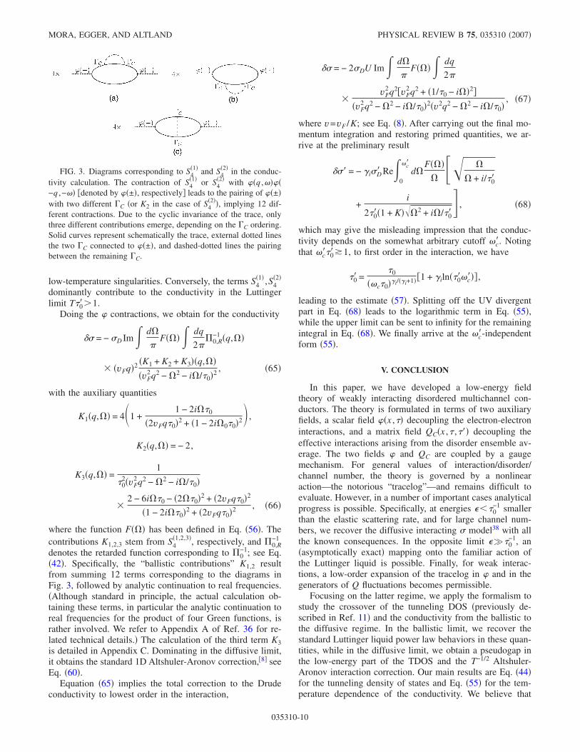
FIG. 3. Diagrams corresponding to S4�1� and S4

�2� in the conduc-tivity calculation. The contraction of S4

�1� or S4�2� with ��q ,��

−q ,−�� denoted by ��±�, respectively� leads to the pairing of ��±�with two different �C �or K2 in the case of S4

�2��, implying 12 dif-ferent contractions. Due to the cyclic invariance of the trace, onlythree different contributions emerge, depending on the �C ordering.Solid curves represent schematically the trace, external dotted linesthe two �C connected to ��±�, and dashed-dotted lines the pairingbetween the remaining �C.


035310-10

these results, covering the entire crossover from ballistic todiffusive, will be valuable in understanding experimentaldata on nanotubes or nanowires.

Let us conclude by noting some of the open problems inthis area. The question of what happens to the conductivity atvery low T cannot be answered by our lowest-order calcula-tion. Relatedly, in order to treat the small-N limit, new con-ceptual advances will be necessary. �Progress along this linehas been reported in Ref. 18.� Other interesting open ques-tions not addressed here include the weak localization cor-rection and the magnetoconductivity, the inclusion of thespin degree of freedom, and a microscopic calculation of thedephasing time in 1D. These topics may be addressed byfuture work.

ACKNOWLEDGMENTS

A. A. thanks J. S. Meyer and A. V. Andreev for discus-sions. This work was supported by the DFG-SFB Transregio12 and by the ESF program INSTANS.

APPENDIX A: DERIVATION OF THE EFFECTIVEMODEL HAMILTONIAN

In this appendix we review how the model Hamiltonian�1� may be distilled from more microscopic descriptions of aquasi-1D conductor. Generally, the simplifying assumptionsbelow are expected to hold for energies ��, where �� isthe characteristic energy scale related to transversal �to thecross section of the wire� excitations in the system. For l�L�, we have ��vF /L�, where L� is a typical transversewidth of the wire. For l�L�, on the other hand, ��

�vFl /L�2 . Resolving phenomena on larger energy scales is a

doable task which, however, requires a more refined �andless universal� modeling. Throughout, the phrase “low en-ergy” refers to the regime ��.

In the absence of disorder and interactions, a quasi-1Dconductor is characterized by N open channels energeticallybelow the Fermi energy. The number N�S� /�F

2 is often tun-able, e.g., via doping or backgate voltages, where S�=L�

2 .We assume that �i� N�1 is sufficiently large to justify theapproximations employed later on and �ii� the Fermi energyis located sufficiently far away from the bottom of the bandsformed by longitudinal momentum components to justify in-troduction of well-defined chiral �right- or left-moving, C=R /L=±� electron branches for each channel; clearly, thisbecomes problematic if the Fermi energy is close to the bot-tom of a band. Moreover, we shall �iii� focus on the case ofspinless �or spin-polarized� electrons. The generalization tothe spinful case does not pose conceptual problems and isleft to future work.

Denoting the 1D coordinate as x �where we assume thatno confinement along this axis is present� and the transversedegrees of freedom as r�, the electron operator �e�r�, withr= �x ,r��, can be expanded into the N transverse eigenfunc-tions as

�e�r� = �n=1

N

�C=R/L

eiCknx�n�r��nC�x� , �A1�

where �n�r�� are the transverse eigenmodes normalized ac-cording to

� dr��n*�r��m�r�� = nm. �A2�

To give an example, for MWNTs, the eigenmodes, arisingfrom the wrapping of a 2D graphene sheet onto a cylinder,are27

�n�y� = L�−1/2exp�2�iny/L�� , �A3�

where L�=2�R0 for outermost-shell radius R0 of theMWNT. Here the transverse coordinate is the angular vari-able y, with 0�y�L�. For given confinement, each bandintersects the Fermi surface at k= ±kn with its own Fermimomentum kn, where the slope is given by the respectiveFermi velocity vn. At low energy scales, the kinetic part ofthe Hamiltonian then is

H0 = − i�C

C� dx �C† �x�v�x�C�x� , �A4�

with v=diag�v1 ,v2 , . . . ,vN�. The noninteracting DOS is thusgiven by �1=�n=1

N 1/ ��vn�. To simplify matters, we neglectdifferences in the channel-dependent velocity, vn→ �vn�n

�vF, where vF denotes the average channel velocity. As maybe checked, e.g., by an explicit calculation of the diffusivetwo-point correlation function of the system, this assumptionis permissible at low energies. For equal Fermi velocities, thekinetic part of the Hamiltonian assumes the form of H0 inEq. �1�.

Next let us turn to the repulsive Coulomb interactionsamong the electrons in the QW. Starting from an arbitrarymicroscopic interaction potential Umicr�r ,r��, which incorpo-rates external screening effects due to the substrate or sur-rounding gates, one arrives at a rather complicated 1D inter-action Hamiltonian. At low energies, it is however sufficientto consider a simple model interaction, which is assumed tobe long-ranged �e.g., a 1 /r potential� on length scales largerthan L�. In that case, the long-range tail of the interaction isexpected to dominate all relevant 1D Coulomb interactionmatrix elements, such as

Unm�x − x�� =� dr�dr�� Umicr�x − x�,r�,r��

� ��n�r��2��m�r�� 2.

For �x−x� � �L�, the potential Umicr is basically independentof the transverse coordinates r� and r�� , implying that theprojected interaction does not depend on the channel indices,Umn→U�x−x��. The expansion �A1� then leads to an effec-tive contribution to the Hamiltonian,

HI =1

2 �n,m=1

N

�C1,C2,C3,C4

� dx dx�U�x − x��

� e−i�C1−C4�knxe−i�C2−C3�kmx�

� �nC1

† �x��mC2

† �x��mC3�x��nC4

�x� . �A5�

Following the standard reasoning leading to LL models,1,2

for a long-ranged potential, electron-electron �e-e� back-scattering �C1=−C4 ,C2=−C3� processes will be strongly


035310-11

suppressed. Moreover, e-e Umklapp scattering is importantonly close to commensurabilities and will not be discussedhere. For a long-ranged interaction, the dominant interactionprocess then corresponds to e-e forward scattering, whereC1=C4 and C2=C3 in Eq. �A5�. Such processes describeinteractions coupling the 1D density fluctuations, HI

= 12 �dx dx��x�U�x−x��x��. It is then justified to express

HI in terms of the q=0 Fourier component of U�x−x��, de-noted by U. �In the clean case, up to multiplicative logarith-mic corrections in most observables, this procedure also de-scribes the case of the unscreened 1/r interaction.1� We arethen left with the simple 1D forward-scattering interaction�6�. We mention in passing that e-e backscattering can be�partially� included by allowing for different interactionstrengths g4 and g2 in the CC and C−C couplings,respectively.1 With minor modifications, our approach can beadjusted to this situation.

Finally, quenched disorder is included by starting from ashort-ranged �3D� Gaussian random potential V�r�, with thedisorder average defined by its only nonvanishing cumulant

�V�r�V�r��dis =1

2��3�0�r − r�� , �A6�

where �3=�1 /S� is the 3D noninteracting DOS and we as-sume that disorder is weak, knl�1 for all kn. With Eq. �A1�,we then obtain FS and BS scattering as in Eqs. �3� and �4�,respectively, where

VC,nn� = e−iC�kn−kn��x� dr��n*�r��n��r��V�r� ,

Wnn� = e−i�kn+kn��x� dr��n*�r��n��r��V�r�

can be taken as independent random variables whose statis-tical properties follow from Eq. �A6�. To simplify matters,we assume the specific torus-type confinement �A3�. Unlessone is interested in details of transverse fluctuations or otherhigh-energy features, the precise form of the confinementpotential is not expected to change the essential physics. Sta-tistical correlations of Wnm�x� can then be described by thesimple form �5�.

APPENDIX B: NONINTERACTING LIMIT OF THE NL�M

Let us discuss here the diffusive properties at�q � l�1, ��m ��0�1 of the NL�M �38� in the noninteractinglimit. Using the parametrization �33�, we have two differenttypes of quantum fluctuations, B0 and B1, where the latterbreak chiral symmetry. The B1 modes have a gap, but nev-ertheless are not to be discarded since they couple to themassless B0 fluctuations. We show this now on the Gaussianlevel, starting from the noninteracting version of Eq. �38�,

S =��1

8�0Tr�QRQL� +

��1

4 �C

Tr�D��xQC�2

+ 2C��TC−1�xTC� − 2�QC� , �B1�

where we put vF=1 in intermediate steps. In order to recover

the conventional NL�M, we define the chirally symmetricfield Q0=T0�T0

−1 with T0=exp�−W0 /2�, and integrate overthe massive modes B1. Expanding S to second order in B1�but zeroth order in B0�, the first term in Eq. �B1� produces

−��1

4�0Tr�W1

2� =��1

2�0Tr�B1

†B1� ,

see Eq. �34�, which determines the mass gap of the fluctua-tion mode B1 referred to in Sec. II B. The remaining parts ofthe action �B1� are then expanded to linear order in B1,where only the TC

−1�xTC term gives a contribution. Here onehas to be careful because of the noncommuting nature ofB0,1, but within a first-order expansion, no difficulties ariseunder the parametrization �33�. Terms that are quadratic inB1 or involve spatial derivatives of B1 are neglected sincethey vanish at low energy and/or long length scales. We fi-nally arrive at

S =��1

2Tr„D��xQ0�2 − 2�Q0 − W1

2/2�0 − iW1�T0−1�xT0,��−… .

Next B1 is integrated out, and we finally obtain the 1D dif-fusive action for Q0,

S =��1

4„D Tr��xQ0�2 − 4 Tr��Q0�… . �B2�

On the Gaussian level, keeping replica indices implicit, thisresults in

S =��1T2

2 ��n�0,�m�0

� dq

2��Dq2 + ��n − �m��B0;nm�q��2,

implying the usual diffusion pole.We finally remark that at energies ��, the diffusion

properties �e.g., of MWNTs� become anisotropic. These “me-dium energy effects” may be resolved by employing the fulldisorder correlator of the Wnm�x�, and decoupling the impu-rity four-fermion action in terms of a channel-dependent Qfield. One thus obtains a more structured theory wherein de-tails of anisotropic transport are resolved.

APPENDIX C: INTERACTION CORRECTION

Here we provide the derivation of S4�3� and of the corre-

sponding interaction correction; see Sec. IV B. The expan-sion of Eq. �32� in B yields

SB =��1

8�0Tr�W1�3W1 + W0�1W0

− W0�2W1 + 2W0P0 + 2W1P1� ,

with kernels

�1�q,�� =vF

2q2 + �� + 1/2�0�vF

2q2 + �� + 1/2�0�2 ,

�2�q,�� =qvFsgn��/�0

vF2q2 + �� + 1/2�0�2 ,


035310-12

�3�q,�� =�� + 1/�0�� + 1/2�0� + vF

2q2

vF2q2 + �� + 1/2�0�2 .

Moreover,

P0�q0,�n,�n − �0� = �C,�m

� dq

2��C�q,�m��C�q0 − q,�0

− �m�IC�q,�m,q0,�0� + K2�q,�m�K2�q0

− q,�0 − �m�sgn��n − �m�� ,

and

P1�q0,�n,�n − �0� = �C,�m

�− iC� � dq

2��C�q,�m�

��C�q0 − q,�0 − �m�IC�q,�m,q0,�0�� ,

with the kernel

IC�q,�m,q0,�0� = ivF� dp

2�GC�p,��

�GC�p − q0,� − �0�GC�p − q,� − �m� .

The Gaussian B fluctuations are then integrated out. Callingthe resulting action S4

�3�, we find

S4�3� = −

��1

4�0�

q0,q1,q2

��0�0,�1,�2

�0��n��0

� �C

�C�q1,�1��C�q0 − q1,�0 − �1�IC�q0,�0,q1,�1��1 −iC

4

�2�q0,�0��3�q0,�0��

+ K2�q1,�1�K2�q0 − q1,�0 − �1�sgn��n − �1�� C�

�C��q2,�2��C��− q0 − q2,− �0 − �2�IC��q0,�0,q0 + q2,�0 + �2�

��1 −iC�

4

�2�q0,�0��3�q0,�0�� + K2�q2,�2�K2�− q0 − q2,− �0 − �2�sgn��n − �0 − �2��„�1�q0,�0� − �2

2�q0,�0�/4�3�q0,�0�…−1

+ �C

�− iC��C�q1,�1��C�q0 − q1,�0 − �1�IC�q0,�0,q1,�1��

C�

�− iC��C��q2,�2��C��q0 − q2,�0 − �2�IC��q0,�0,q0 + q2,�0 + �2��3�q0,�0�� .

Equation �64� is then used to compute the conductivity cor-rection. The contraction of ��q ,��−q ,−�� with S4

�3� leadsto eight terms, with four different terms appearing twiceeach. These four terms are in fact two by two equivalent viathe symmetry �→−�. In particular, the two contributionswith −� vanish after the summation over �n is performed.The two possible contractions are �i� q1=−q2=q, �1=−�2=� and �ii� q1=q, �1=�, q2=q−q0, �2=�−�0. The externalmomentum q is now taken to zero, and we also let �→0under the constraint Re ��0. The �n summation can bedone easily and yields, after the frequency shift �0→�0+�m,

�3 = −8vF

2e2�1�03

�m�

�0�0,q0

�0 + �m − ��0 − �m��0�q0,�0�

��X12�q0,�0�„�1�q0,�0� − �2

2�q0,�0�/4�3�q0,�0�…−1

+ X22�q0,�0�/�3�q0,�0�� ,

where �m→0 has been anticipated and we have used theabbreviations

X1�q0,�0� =1

4�02�

C

C�C�q0,�0�2ivFq0��q0,�0�

��1 −iC

4

�2�q0,�0��3�q0,�0��IC

0 �q0,�0�

+i

2�0

K2�q0,�0�ivFq0��q0,�0�

,

X2�q0,�0� =1

4�02�

C

�− i��C�q0,�0�2ivFq0��q0,�0�

IC0 �q0,�0� ,

IC0 �q0,�0� = 2�0

1/�0 + �0 − iCvFq0

�1/2�0 + �0 − iCvFq0�2 .

The summation over �0 is then replaced by a contour inte-gral, with a line cut for �= i�0= i�. Performing the analyticcontinuation i�=��+ i0+ with ��→0, we finally obtain K3in Eq. �65�.


035310-13

1 A. O. Gogolin, A. A. Nersesyan, and A. M. Tsvelik, Bosonizationand Strongly Correlated Systems �Cambridge University Press,Cambridge, UK, 1998�.

2 J. Voit, Rep. Prog. Phys. 58, 977 �1995�.3 C. L. Kane and M. P. A. Fisher, Phys. Rev. B 46, 15233 �1992�.4 D. C. Mattis, Phys. Rev. Lett. 32, 714 �1974�.5 A. Luther and I. Peschel, Phys. Rev. Lett. 32, 992 �1974�.6 W. Apel and T. M. Rice, Phys. Rev. B 26, R7063 �1982�.7 S. Andergassen, T. Enss, V. Meden, W. Metzner, U. Schollwöck,

and K. Schönhammer, Phys. Rev. B 70, 075102 �2004�.8 B. L. Altshuler and A. G. Aronov, in Electron-Electron Interac-

tions in Disordered Solids, edited by A. L. Efros and M. Pollak�Elsevier, Amsterdam, 1985�.

9 A. Kamenev and A. Andreev, Phys. Rev. B 60, 2218 �1999�.10 Yu. V. Nazarov, JETP Lett. 49, 126 �1989�; Sov. Phys. JETP 68,

561 �1989�.11 E. G. Mishchenko, A. V. Andreev, and L. I. Glazman, Phys. Rev.

Lett. 87, 246801 �2001�.12 G. Grüner, Density Waves in Solids �Addison-Wesley, Reading,

MA, 1994�.13 T. Giamarchi and H. J. Schulz, Phys. Rev. B 37, 325 �1988�.14 A. Furusaki and N. Nagaosa, Phys. Rev. B 47, 4631 �1993�.15 M. Ogata and H. Fukuyama, Phys. Rev. Lett. 73, 468 �1994�.16 N. P. Sandler and D. L. Maslov, Phys. Rev. B 55, 13808 �1997�.17 S. V. Malinin, T. Nattermann, and B. Rosenow, Phys. Rev. B 70,

235120 �2004�.18 I. V. Gornyi, A. D. Mirlin, and D. G. Polyakov, Phys. Rev. Lett.

95, 046404 �2005�; 95, 206603 �2005�.19 K. A. Matveev and L. I. Glazman, Phys. Rev. Lett. 70, 990

�1993�.20 Once interchain hopping becomes relevant, coherent electron

transfer among the chains is important and eventually induces acrossover into a Fermi liquid state. Such effects are implicitlycontained in the model studied below, since the N “open chan-nels” directly represent the eigenmodes of the noninteractingclean system.

21 A. Bachtold, M. de Jonge, K. Grove-Rasmussen, P. L. McEuen,M. Buitelaar, and C. Schönenberger, Phys. Rev. Lett. 87,166801 �2001�.

22 K. Liu, P. Avouris, R. Martel, and W. K. Hsu, Phys. Rev. B 63,161404�R� �2001�.

23 E. Graugnard, P. J. de Pablo, B. Walsh, A. W. Ghosh, S. Datta,and R. Reifenberger, Phys. Rev. B 64, 125407 �2001�.

24 R. Tarkiainen, M. Ahlskog, J. Penttila, L. Roschier, P. Hakonen,M. Paalanen, and E. Sonin, Phys. Rev. B 64, 195412 �2001� R.Tarkiainen, M. Ahlskog, M. Paalanen, A. Zyuzin, and P. Ha-konen, ibid. 71, 125425 �2005�.

25 N. Kang, J. S. Hu, W. J. Kong, L. Lu, D. L. Zhang, Z. W. Pan,and S. S. Xie,Phys. Rev. B 66, 241403�R� �2002�.

26 A. Kanda, K. Tsukagoshi, Y. Aoyagi, and Y. Ootuka, Phys. Rev.Lett. 92, 036801 �2004�.

27 R. Egger and A. O. Gogolin, Phys. Rev. Lett. 87, 066401 �2001�.28 L. Bartosch and P. Kopietz, Eur. Phys. J. B 28, 29 �2002�.29 T. Lorenz et al., Nature �London� 418, 614 �2002�.30 E. Slot, M. A. Holst, H. S. J. van der Zant, and S. V. Zaitsev-

Zotov, Phys. Rev. Lett. 93, 176602 �2004�.31 A. N. Aleshin, H. J. Lee, Y. W. Park, and K. Akagi, Phys. Rev.

Lett. 93, 196601 �2004�.32 F. Liu, M. Bao, K. L. Wang, C. Li, B. Lei, and C. Zhou, Appl.

Phys. Lett. 86, 213101 �2005�.33 L. Venkataraman, Y. S. Hong, and P. Kim, Phys. Rev. Lett. 96,

076601 �2006�.34 K. A. Matveev, D. Yue, and L. I. Glazman, Phys. Rev. Lett. 71,

3351 �1993�.35 A. M. Rudin, I. L. Aleiner, and L. I. Glazman, Phys. Rev. B 55,

9322 �1997�.36 G. Zala, B. N. Narozhny, and I. L. Aleiner, Phys. Rev. B 64,

214204 �2001�.37 I. V. Gornyi and A. D. Mirlin, Phys. Rev. Lett. 90, 076801

�2003�.38 A. M. Finkel’stein, Sov. Phys. JETP 57, 97 �1983�.39 D. S. Golubev and A. D. Zaikin, Phys. Rev. B 70, 165423 �2004�.40 D. S. Golubev, A. V. Galaktionov, and A. D. Zaikin, Phys. Rev. B

72, 205417 �2005�.41 The reason for avoiding bosonization is that a straightforward

multichannel generalization of the bosonized theory �Ref. 13�does not properly describe the diffusive phase in the noninter-acting limit. Technically, this failure can be traced to a breakingof the replica rotation symmetry originally present in the nonin-teracting model, yet absent in the �Abelian� bosonized theory�Ref. 13�. For related comments, see also Ref. 18.

42 For channel-dependent interactions beyond Eq. �6�, and for non-uniformly distributed Fermi velocities, additional terms may begenerated. However, we do not believe these terms to be ofphysical relevance. Specifically, on the noninteracting level, andindependent of fluctuations in the Fermi velocities, the correct�anisotropic� diffusion properties are recovered from impuritybackscattering alone.

43 J. Zinn-Justin, Quantum Field Theory and Critical Phenomena,4th ed. �Oxford University Press, Oxford, 2002�.

44 K. Fujikawa and H. Suzuki, Phys. Rep. 398, 221 �2004�.45 In the diagrammatic approach, the disordered Green function has

a 1/2�0 prefactor before �, in contrast to Eq. �28�. The differ-ence arises here quite naturally.

46 There is an additional prefactor K1/N in Eq. �44�, which we drophere. For N�1 and �1U�1, it is very close to unity.

47 I. S. Gradshteyn and I. M. Ryzhik, Table of Integrals, Series, andProduct �Academic Press, New York, 1980�.

48 A. Bachtold, M. S. Fuhrer, S. Plyasunov, M. Forero, E. H. Ander-son, A. Zettl, and P. L. McEuen, Phys. Rev. Lett. 84, 6082�2000�.


035310-14

Documents

From Luttinger liquid to Altshuler-Aronov anomaly in multichannel quantum wires