Embed Size (px)
Citation preview
CER
N-T
HES
IS-2
016-
438
06/0
7/20
16
Master Thesis
Cooling Circuit Designfor the Large-Scale Liquid Argon Detectors
in the ICARUS Experiment
Hannah Kirsch
06.07.2016
Supervision: Dr. Torsten Koettig, CERN
Assignment: Prof. Dr.-Ing. Steffen Grohmann, KIT
Second Corrector: Prof. Dr.-Ing. Dr. h. c. Wilhelm Schabel, KIT
Institute of Technical Thermodynamicsand Refrigeration
KIT - university of the state of Baden-Württemberg andnational research center of the Helmholtz Association


ii
Selbständigkeitserklärung
Hiermit erkläre ich, dass ich folgende Arbeit selbständig verfasst und keine anderen als dievon mir angegebenen Quellen und Hilfsmittel benutzt habe, die wörtlich oder inhaltlichübernommene Stellen als solche kenntlich gemacht und die Satzung des Karlsruher Insti-tuts für Technologie (KIT) zur Sicherung guter wissenschaftlicher Praxis in der jeweilsgültigen Fassung beachtet habe. Ich erkläre mich damit einverstanden, dass die Arbeit indie Bibliothek eingestellt und kopiert werden darf.
Datum Unterschrift

iv

Acknowledgements
First of all, I would like to express my sincere gratitude to Professor Grohmann. He en-couraged me to participate in the Technical Student Programme at CERN and supportedmy application. By his personal support he made this external Master Thesis possible.
Special thanks also goes to my supervisor at CERN, Dr. Torsten Koettig. He made iteasy to feel at home at the Cryolab. I really appreciated his vivid introduction into theworld of particles and accelerators as well as cryogenics. His theoretical and practical sup-port was crucial for this work.
Moreover, many thanks to all the staff, PhD students, fellows, students and technicians ofthe Cryolab I met during my stay at CERN. Here, in particular, Dario Santandrea shouldbe mentioned, with whom I worked together on the ICARUS project.

vi
Zusammenfassung
Der ICARUS Detektor wurde entwickelt, um Neutrinos zu detektieren und das Phäno-men der Neutrinooszillation näher zu untersuchen. Der Detektor wird mit flüssigem Ar-gon gefüllt und arbeitet bei Umgebungsdruck, wodurch die Temperatur des Detektorsauf die Sättigungstemperatur des Argons von 87 K festgelegt ist. Damit die Wechselwir-kungen zwischen den Neutrinos und den Argon Atomen möglichst genau rekonstruiertwerden können, müssen Temperaturgradienten innerhalb des Argons und die daraus re-sultierenden Konvektionen minimiert werden. Daher ist der ICARUS Detektor mit einemthermischen Schild, das nahezu den ganzen Wärmeeintrag aus der Umgebung abschirmt,ummantelt. Das thermische Schild wird mit siedendem Stickstoff auf Detektortemperaturgekühlt. Das Kühlsystem des thermischen Schildes arbeitet bei einem Druck von 2,8 bar,was dem Sättigungsdampfdruck von Stickstoff bei 87 K entspricht. Als Kühlmittel wurdeStickstoff im Siedezustand gewählt, da in erster Näherung bei Annahme einer druckverlust-freien Strömung die Temperatur während des Verdampfens des Stickstoffs konstant bleibt.Ein Druckverlust einer Strömung im Zweiphasengebiet ist jedoch immer mit einem Tem-peraturabfall korreliert. Aus diesem Grund ist es wichtig, den Druckverlust der Stickstoff-Zweiphasenströmung über die Länge des Kühlsystems genau bestimmen zu können.Im Rahmen dieser Masterarbeit wird der Druckverlust einer Stickstoff-Zweiphasenströ-
mung unter den Bedingungen, wie sie später im thermischen Schild auftreten werden, un-tersucht. Dies entspricht einem Druck von 2,8 bar, Massenstromdichten von 20 kg m−2 s−1
bis 70 kg m−2 s−1 und Gasgehalten bis zu 70 %. Da die Wechselwirkungen der Gas- undder Flüssigphase einer Zweiphasenströmung noch nicht vollständig verstanden sind, basie-ren viele in der Literatur dargestellten Duckverlustkorrelationen auf empirischen Daten,was deren Übertragbarkeit auf andere Fluide sowie Drücke und Massenstromdichten ein-schränkt. Die berechneten Druckverluste der Stickstoff-Zweiphasenströmung über die Län-ge des thermischen Schildes mit Hilfe verschiedener ausgewählter Korrelationen aus derLiteratur weichen stark voneinander ab. Dies unterstreicht die Notwendigkeit, den Druck-verlust im Bereich der interessierenden Bedingungen experimentell zu untersuchen.Nach einer kurzen Einführung in die Physik der Neutrinos und in das Konzept des
ICARUS Detektors werden die theoretischen Grundlagen einer Zweiphasenströmung ins-besondere des Druckverlustes in der Zweiphasenströmung behandelt. Es wird ein Überblick
viii
über einige in der Literatur existierende empirische Korrelationen für den Gasanteil undden Reibungsdruckverlust gegeben. Das nächste Kapitel beschreibt das in Matlab R© entwi-ckelte mathematische Modell um den Druckverlust von Stickstoff-Zweiphasenströmungenim Druckbereich von 2,6 bar bis 2,9 bar zu berechnen. Das Programm koppelt die Ener-gieerhaltungsgleichung mit der Impulserhaltungsgleichung, um dem Phänomen Rechnungzu tragen, dass sich der Gasgehalt einer Zweiphasenströmung sogar unter adiabatischenBedingungen aufgrund des Druckverlustes über die Rohrlänge ändert. Im Mittelpunkt desdarauffolgenden Kapitels steht der Versuchsaufbau zur Bestimmung des Druckverlusteseiner siedenden Stickstoffströmung unter den oben genannten Bedingungen. Die Teststre-cke wird unter quasi-adiabatischen Bedingungen betrieben und setzt sich aus einem ho-rizontalen, einem vertikal aufwärtsgerichteten und einem vertikal abwärtsgerichteten Teilzusammen. Die erhaltenen Messdaten stellen eine erste Datenbank für den Druckverlustvon Stickstoff im Zweiphasengebiet unter den oben genannten Bedingungen dar. Durcheinen Vergleich der Messdaten mit den berechneten Daten aus dem Matlab R© Programmwird die Korrelation für den Gasanteil und den Reibungsdruckverlust der untersuchtenStickstoff-Zweiphasenströmung bestimmt, die die Messdaten mit der geringsten Abwei-chung wiedergibt. Die Korrelation nach Rouhani für den Gasgehalt sowie das Modell nachMüller-Steinhagen und Heck für den Reibungsdruckverlust bilden am besten die gemesse-nen Daten für eine horizontale Strömung oder vertikale Aufwärtsströmung ab. Bei verti-kaler Abwärtsströmung tritt, im Gegensatz zu der Berechnung, in den gemessenen Wertenkeine Drucksteigerung auf. Zudem wird das Abkühlverhalten des Versuchsaufbaus aus-gehend von Raumtemperatur untersucht. Im letzten Teil dieser Arbeit werden die durchden Versuchsaufbau erhaltenen Erkenntnisse angewendet, um den Druckverlust im realenKühlsystem des thermischen Schildes des ICARUS Detektors zu berechnen und ein Vor-schlag für die Gestaltung des Kühlsystems wird unterbreitet. Das Kühlsystem kann dieForderung nach einem Temperaturgradienten von maximal 500 mK einhalten. Da sich inkryogenen Systemen bei ungewolltem Wärmeeintrag hohe Drücke aufbauen können, wer-den die an die erforderlichen Sicherheitsvorkehrungen gegen exzessiven Überdruck in Formvon Sicherheitsventilen oder Berstscheiben gesetzten Anforderungen betrachtet.
Contents
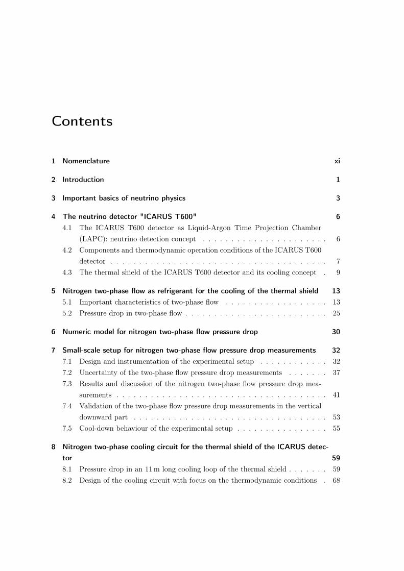
1 Nomenclature xi
2 Introduction 1
3 Important basics of neutrino physics 3
4 The neutrino detector "ICARUS T600" 64.1 The ICARUS T600 detector as Liquid-Argon Time Projection Chamber
(LAPC): neutrino detection concept . . . . . . . . . . . . . . . . . . . . . . 64.2 Components and thermodynamic operation conditions of the ICARUS T600
detector . . . . . . . . . . . . . . . . . . . . . . . . . . . . . . . . . . . . . . 74.3 The thermal shield of the ICARUS T600 detector and its cooling concept . 9
5 Nitrogen two-phase flow as refrigerant for the cooling of the thermal shield 135.1 Important characteristics of two-phase flow . . . . . . . . . . . . . . . . . . 135.2 Pressure drop in two-phase flow . . . . . . . . . . . . . . . . . . . . . . . . . 25
6 Numeric model for nitrogen two-phase flow pressure drop 30
7 Small-scale setup for nitrogen two-phase flow pressure drop measurements 327.1 Design and instrumentation of the experimental setup . . . . . . . . . . . . 327.2 Uncertainty of the two-phase flow pressure drop measurements . . . . . . . 377.3 Results and discussion of the nitrogen two-phase flow pressure drop mea-
surements . . . . . . . . . . . . . . . . . . . . . . . . . . . . . . . . . . . . . 417.4 Validation of the two-phase flow pressure drop measurements in the vertical
downward part . . . . . . . . . . . . . . . . . . . . . . . . . . . . . . . . . . 537.5 Cool-down behaviour of the experimental setup . . . . . . . . . . . . . . . . 55
8 Nitrogen two-phase cooling circuit for the thermal shield of the ICARUS detec-tor 598.1 Pressure drop in an 11m long cooling loop of the thermal shield . . . . . . . 598.2 Design of the cooling circuit with focus on the thermodynamic conditions . 68
x Contents
8.3 Pressure safety analysis and required safety devices . . . . . . . . . . . . . . 71
9 Conclusion 80
List of Tables 82
List of Figures 83
Bibliography 87
A Components of the small-scale experimental setup B
B Matlab R© program E
C Correlations used for two-phase flow pressure drop G

1 Nomenclature
A cross-section (m2)
C flow coefficient (-)
C0 parameter drift-flux model (-)
cp specific heat capacity ( Jkg·K )
d inner diameter (m)
f friction factor (-)
FD parameter flow pattern map Taitel and Dukler (-)
g acceleration due to gravity (ms2 )
G mass flow density / mass velocity ( kgm2·s )
h enthalpy ( Jkg )
i momentum flow density / momentum velocity ( kgm·s2 )
J volumetric flow density / volumetric velocity ( m3
m2·s )
KD parameter flow pattern map Taitel and Dukler (-)
Kd safety valve discharge coefficient (-)
L length (m)
m mass flow (kgs )
N boiling delay factor (-)
P power (W)
p pressure (bar)
T temperature (K)
q heat flux ( Wm2 )
Q heat flow (W)
Re Reynolds number (-)
S slip ratio (ratio of velocity vapour phase to velocity liquid phase) (-)
t time (s)
u velocity (ms )
uvj parameter drift-flux model (ms )
v specific volume (m3
kg )
V volumetric flow (m3
s )
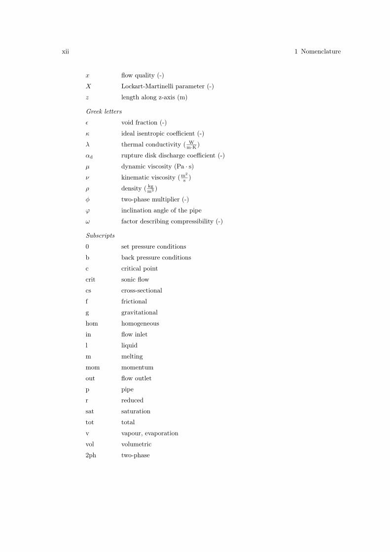
xii 1 Nomenclature
x flow quality (-)
X Lockart-Martinelli parameter (-)
z length along z-axis (m)
Greek letters
ε void fraction (-)
κ ideal isentropic coefficient (-)
λ thermal conductivity ( Wm·K )
αd rupture disk discharge coefficient (-)
µ dynamic viscosity (Pa · s)ν kinematic viscosity (m
2
s )
ρ density ( kgm3 )
φ two-phase multiplier (-)
ϕ inclination angle of the pipe
ω factor describing compressibility (-)
Subscripts
0 set pressure conditions
b back pressure conditions
c critical point
crit sonic flow
cs cross-sectional
f frictional
g gravitational
hom homogeneous
in flow inlet
l liquid
m melting
mom momentum
out flow outlet
p pipe
r reduced
sat saturation
tot total
v vapour, evaporation
vol volumetric
2ph two-phase
2 Introduction
CERN, whose name originally derived from Conseil Européen pour la Recherche Nucléaire,is the European Organization for Nuclear Research located along the French-Swiss bordernear Geneva. CERN was founded in the year 1954 as Europe’s first joint venture andnowadays belongs to the best research organizations for particle physics around the globe.Physicists as well as engineers are dedicated to explore the fundamental structure of ouruniverse - the constituents of matter and the forces between them. A complex of particleaccelerators increases the speed of particles almost to the speed of light and let them collidepurposely. Detectors provide information about the particle interactions and the releasedfragments. The technology used is at the forefront of science combining knowledge from21 member states and many collaborations.[1]A collaboration between the US Fermi National Accelerator Laboratory (Fermilab),
the Italian Institute for Nuclear Physics (INFL) and CERN is currently working on theICARUS neutrino experiment. The large-scale ICARUS T600 detector is designed to befilled with liquid argon and to detect neutrinos allowing research in the field of neutrino os-cillations [2]. The Cryolab at CERN was assigned the task to investigate the details of thethermal shield design for the ICARUS T600 detector taking into account the constraintsgiven by the experiment. The thermal shield is actively cooled with boiling nitrogen andoperates at a pressure of 2.8 bar, which corresponds to a saturation temperature of 87 K.The thermal shield should have a temperature gradient less than 500 mK. Theoretically,not considering the pressure drop along the cooling circuit, the temperature stays constantduring evaporation in the chosen two-phase flow regime. The only temperature change iscaused by the small pressure drop along the cooling loop. Due to the strict temperatureconstraints, it is important to study the pressure drop of nitrogen two-phase flow alongthe cooling circuit of the thermal shield in different orientations of the flow in respect togravity.The objective of this master thesis is to investigate the proposed design of the thermal
shield of the ICARUS detector especially the pressure drop along the nitrogen two-phaseflow cooling circuit. After a short introduction to the fundamentals of neutrino physicsand the design of the ICARUS T600 detector, the presented master thesis introduces thedistinctive characteristics of two-phase flow such as flow quality, flow pattern, void fraction
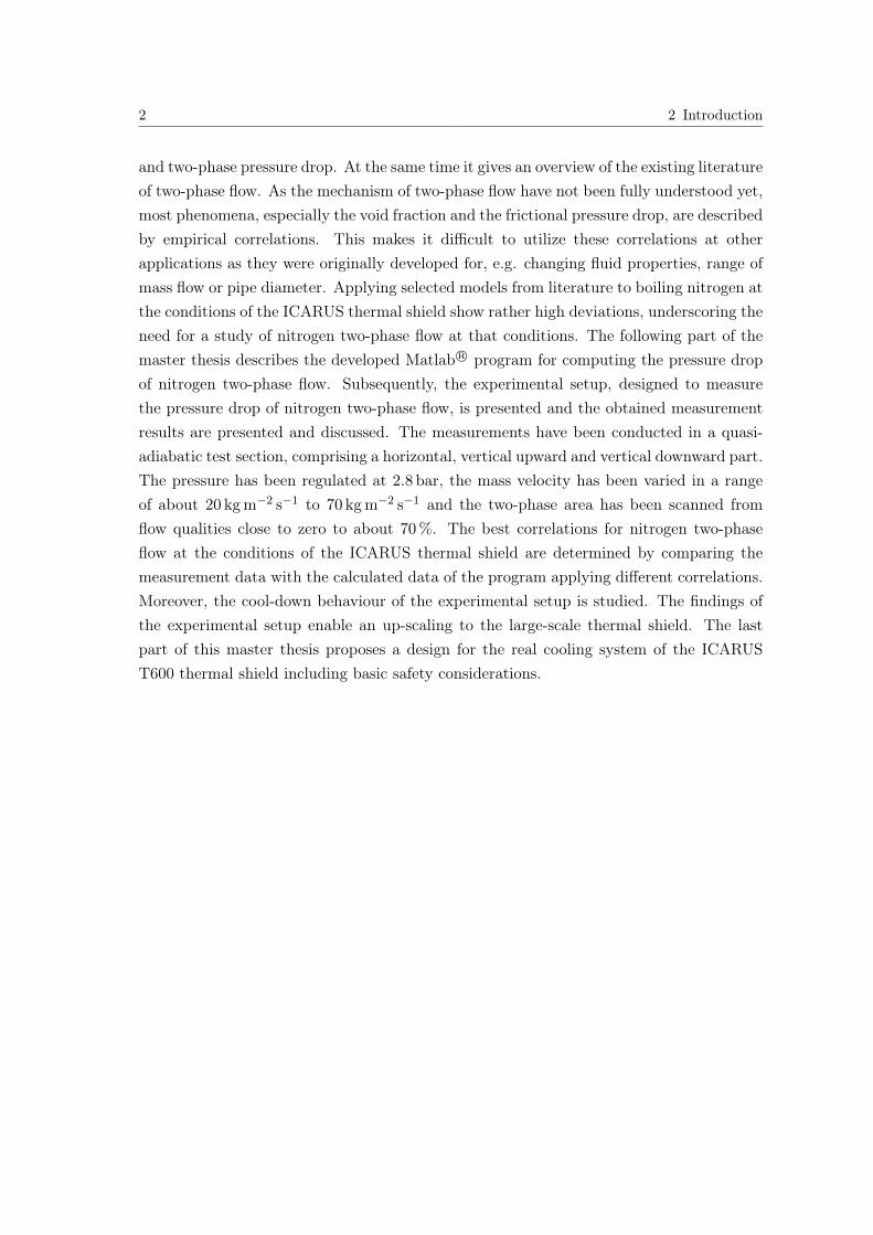
2 2 Introduction
and two-phase pressure drop. At the same time it gives an overview of the existing literatureof two-phase flow. As the mechanism of two-phase flow have not been fully understood yet,most phenomena, especially the void fraction and the frictional pressure drop, are describedby empirical correlations. This makes it difficult to utilize these correlations at otherapplications as they were originally developed for, e.g. changing fluid properties, range ofmass flow or pipe diameter. Applying selected models from literature to boiling nitrogen atthe conditions of the ICARUS thermal shield show rather high deviations, underscoring theneed for a study of nitrogen two-phase flow at that conditions. The following part of themaster thesis describes the developed Matlab R© program for computing the pressure dropof nitrogen two-phase flow. Subsequently, the experimental setup, designed to measurethe pressure drop of nitrogen two-phase flow, is presented and the obtained measurementresults are presented and discussed. The measurements have been conducted in a quasi-adiabatic test section, comprising a horizontal, vertical upward and vertical downward part.The pressure has been regulated at 2.8 bar, the mass velocity has been varied in a rangeof about 20 kg m−2 s−1 to 70 kg m−2 s−1 and the two-phase area has been scanned fromflow qualities close to zero to about 70 %. The best correlations for nitrogen two-phaseflow at the conditions of the ICARUS thermal shield are determined by comparing themeasurement data with the calculated data of the program applying different correlations.Moreover, the cool-down behaviour of the experimental setup is studied. The findings ofthe experimental setup enable an up-scaling to the large-scale thermal shield. The lastpart of this master thesis proposes a design for the real cooling system of the ICARUST600 thermal shield including basic safety considerations.
3 Important basics of neutrino physics
In the year 1930 Wolfgang Pauli postulated the existence of a further lepton today calledneutrino. During studies of the radioactive β−-decay several physicians figured out thatthe generated electrons show a continuous energy spectrum. But if, as previously assumed,during a β−-decay a neutron decays only into a proton and an electron, the energy of theelectron should be constant according to the law of energy conservation. By introducinga third emitted uncharged particle, the neutrino, Pauli was now able to explain the con-tinuous energy spectrum of the electrons. Thus, the released energy of the β−-decay isdistributed between three particles, whereby the sum of the energy of the electron andthe neutrino has to be constant. At one extreme, the electron absorbs the total kineticenergy, whereas the neutrino absorbs no energy. This corresponds to the upper limit of theobserved electron energy spectrum. At the other extreme, the neutrino carries away allthe energy. This corresponds to the lower limit of the observed electron energy spectrum.Finally, in the year 1956 Cowan and Reines succeeded in verifying electron neutrinos emit-ted by a nuclear reactor [3]. The following reaction describes the β−-decay of a neutron(It is not sure if neutrinos are Dirac particles or Majorana particles. In the latter case theparticle and antiparticle would be identical [4]):
n −→ p+ + e− + νe . (3.1)
Neutrinos are abundant. Almost 1011 neutrinos are penetrating the earth per squarecentimetre and second [4]. There are mainly four different natural sources of neutrinos [3]:
• Solar neutrinos of various energy are created by the sequence of nuclear fusion reac-tions in the sun.
• Cosmic neutrinos are generated by the explosion of stars, known as supernova.
• Atmospheric neutrinos are formed when pions, originally released in the particleshower of atmospheric reactions triggered by cosmic rays, decay.
• Reactor neutrinos are evolved by multiple reactions, e.g. β−-decay.
In accelerators and laboratories neutrinos are produced artificially by mostly shootingaccelerated protons with a high energy on a fixed target. The sputtered kaons and pions
4 3 Important basics of neutrino physics
are instable and neutrinos are released in the course of their decay series. One challengeis to focus the beam of neutrinos as the kaons and pions are escaping from the targetmaterial at many different angles. As neutrinos are neutral it is impossible to focus themby the means of electromagnetic fields. The only possibility is to already concentrate thecharged kaons and pions [5]. Nevertheless, neutrinos are not easy to detect as they areuncharged and are only interacting with matter by weak interaction via charged-currentreactions (W-exchange) or neutral-current reactions (Z-exchange) [3].Neutrinos feature some special characteristics. The idea of neutrino oscillations was
first proposed by Pontecorvo in the 1950s [3]. According to the present accepted modelthree different types of neutrinos exist: electron neutrinos νe, myon neutrinos νµ, and tauneutrinos ντ . These so-called flavour states are defined by the following matrix [4]:νe
νµ
ντ
=
Ue1 Ue2 Ue3
Uµ1 Uµ2 Uµ3
Uτ1 Uτ2 Uτ3
·ν1
ν2
ν3
, (3.2)
where each neutrino (νe, νµ, ντ ) is a mixture of different mass states with specified mass(ν1 to ν3). Depending on the mixing proportion of the three mass states the flavour stateis determined. That means, if a neutrino with a specific energy is emitted, the differentmass states of this neutrino will travel at different velocities. Hence, while moving themixture of the mass states is changing and the neutrino forms another flavour state [3].The periodically changing probability of the transformation is described by equation (3.3).The oscillation probability depends on the difference of the squared masses of each state.The more distinct the mass differences are, the higher is the frequency of the oscillation[4].
Pνx→νy = sin2 2θ sin2
(1
4
∆m2xyc4
~c
L
pc
)(3.3)
θ is the Cabbibo angle, ~ is the reduced Planck constant, c is the speed of light, m is themass, p is the momentum and L is the distance the particle travelled.Neutrino oscillation experiments are mostly based on one of the two following funda-
mental principles. There is always a source, which emits a specific flavour of neutrinos,as well as the detector is especially sensitive for one specific flavour state. According toequation (3.3), the probability of neutrino oscillations from one flavour to another dependson the energy of the neutrinos and on the distance between neutrino production and de-tection. By varying these two parameters, the sensitivity of the detector for one specificoscillation process (e.g.: myon neutrino −→ tau neutrino) can be increased maximizingthe probability of that special process with respect to the others. Either one quantifies the
5
disappearance of one flavour state of neutrinos by measuring a lower flux than expected orone quantifies the appearance of one flavour state, which is not generated by the source [5].One of several neutrino detectors is the ICARUS T600 detector, which will be introducedin the next chapter. Last year, Takaaki Kajita and Arthur B. McDonald were awarded theNobel Prize in Physics for their unambiguous evidence of neutrino oscillations [6].Since the last few years physicians have even considered an additional, yet unknown
flavour state of neutrinos. Some data anomalies have been observed in several neutrinooscillation experiments, especially at short distances, too few or too many neutrinos ofone kind with respect to expectations. The potentially new flavour state is designated assterile state as it shows no or very rare interaction with ordinary matter. It should have afar larger mass difference with standard neutrinos and their oscillation probability shouldbe very high at short distances [7].From the oscillation feature another important characteristic of neutrinos can be de-
duced. If neutrinos are oscillating between the different flavour states and equation (3.3)holds, neutrinos, by implication, must possess a mass and the different kinds of neutrinosmust have a different mass. However, it has not been possible so far to measure the exactmass of neutrinos [4]. The mass of all kinds of neutrinos is by a factor 106 smaller than themass of their corresponding charged particles and lies below the threshold of 2.3 eV c−2 forelectron neutrinos, 0.17 MeV c−2 for myon neutrinos and 15.5 MeV c−2 for tau neutrinos[6]. It is assumed that, in correspondence with the mass of the other leptons, the mass ofthe different neutrino flavours is increasing by each generation. That means, the electronneutrino is the lightest and the tau neutrino is the heaviest [6]. If neutrinos have a mass,they could also help to explain the still unsolved problem of dark matter [3].
4 The neutrino detector "ICARUS T600"
The ICARUS T600 detector (”Imaging Cosmic and Rare Underground Signal”) is thelargest Liquid-Argon Time Projection Chamber (LAPC) constructed and functional up tonow. It has been designed to detect neutrinos allowing research in the field of neutrinooscillations. From May 2010 to June 2013 the detector was installed in the undergroundGran Sasso Laboratory, Italy. It collected data from cosmic rays as well as using a beamof myon neutrinos generated at CERN and sent 732 km through the earth to Gran Sasso[7, 8]. The neutrinos at CERN were produced by protons from the SPS (Super ProtonSynchrotron) hitting a beryllium target. The released mesons are decaying into myons andthen into electrons creating mainly myon neutrinos and a fraction of electron neutrinos(concentration of electron neutrinos about 1 − 2 %). Hence, the ICARUS T600 detectoraimed to study mainly oscillations from myon neutrinos to tau neutrinos [5]. It detected2500 neutrinos during the three years of experiments. At the end of 2014 the detectorwas brought to CERN where it is refurbished and upgraded within the WA-104 program.In 2017, the detector will be sent to Fermilab, USA. It is expected to operate within aseries of three detectors at a distance of 600 m from the neutrino beam source, whichproduces neutrinos at lower energy. The forthcoming experiments at Fermilab shouldfurther investigate the phenomena of neutrino oscillations and collect data, which especiallyenable researchers to validate or invalidate the theory of the so-called sterile flavour stateof neutrinos [7, 8].
4.1 The ICARUS T600 detector as Liquid-Argon TimeProjection Chamber (LAPC): neutrino detection concept
The idea of the Liquid-Argon Time Projection Chamber (LAPC) was originally developedby Rubbia in 1977 [9]. It should satisfy the needs for a neutrino detector with a largesensitive mass, which delivers specific information about time, topology and energy of thedetected particle events. The interaction of a neutrino and an argon atom results in anionization of the latter producing an electron and an anion as well as a discharge of photonsat an energy level in the ultraviolet light range. The photons are detected instantly byphotomultipliers and the charged particles are separated by the electric field and drift
4.2 Components and thermodynamic operation conditions of the ICARUS T600 detector 7
towards the electrodes where they are detected. With all these signals a 3-D-image of theparticle tracks is captured and the drift velocity of the electrons is computed providingcalorimetric details of the incident.Rubbia regarded liquid argon as an appropriate target material for neutrinos as listed
below.
• Liquid argon has a high density (ρLAr = 1396 kg m−3 for psat = 1 bar and Tsat = 87 K)enhancing the probability of an interaction with a neutrino.
• Argon is an inert noble gas with a completely filled valence shell. It allows electronsto pass through unimpededly. The high electron mobility is an essential property ofthe target material as otherwise the electrons emitted by a neutrino-argon interactionare recaptured on their way to the cathode and cannot be detected. Consequently,the argon also has to be very pure what brings up the next point.
• Liquid argon is easy to purify as most organic contaminations are frozen out atpsat = 1 bar and Tsat = 87 K. In contrast oxygen, which easily traps electrons, is notfrozen out at T = 87 K because of its low melting point (Tm,O2 = 54 K at p = 1 bar).Therefore, special filters are inserted in the argon cooling circuit to keep the oxygencontent below 0.1 ppb. One possible source of oxygen can be the outgassing of metals.
• Argon is relatively cheap.
• Argon at ambient pressure can be liquefied by liquid nitrogen at a moderate pressureof 2.8 bar.
In contrast, xenon as an additional noble gas with a high density (ρLXe = 2944 kg m−3 forpsat = 1 bar and Tsat = 165 K) is much more expensive and not available at large quantities.Moreover, it cannot simply be liquefied at ambient pressure by liquid nitrogen as thesaturation temperature of xenon at ambient pressure lies above the critical temperatureof nitrogen (Tc,N2 = 126 K, pc,N2 = 34 bar). That would require a transcritical coolingprocess at extreme pressure.
4.2 Components and thermodynamic operation conditions ofthe ICARUS T600 detector
The ICARUS T600 detector is composed of two mirrored modules with the followingdimensions each: width 3.6 m, height of 3.9 m, length 19.6 m. The detector has a capacityof 760 tons (476 tons active mass) of liquid argon. Each module is again divided alongthe long side into two chambers by a cathode, which is hence shared between the two
8 4 The neutrino detector "ICARUS T600"
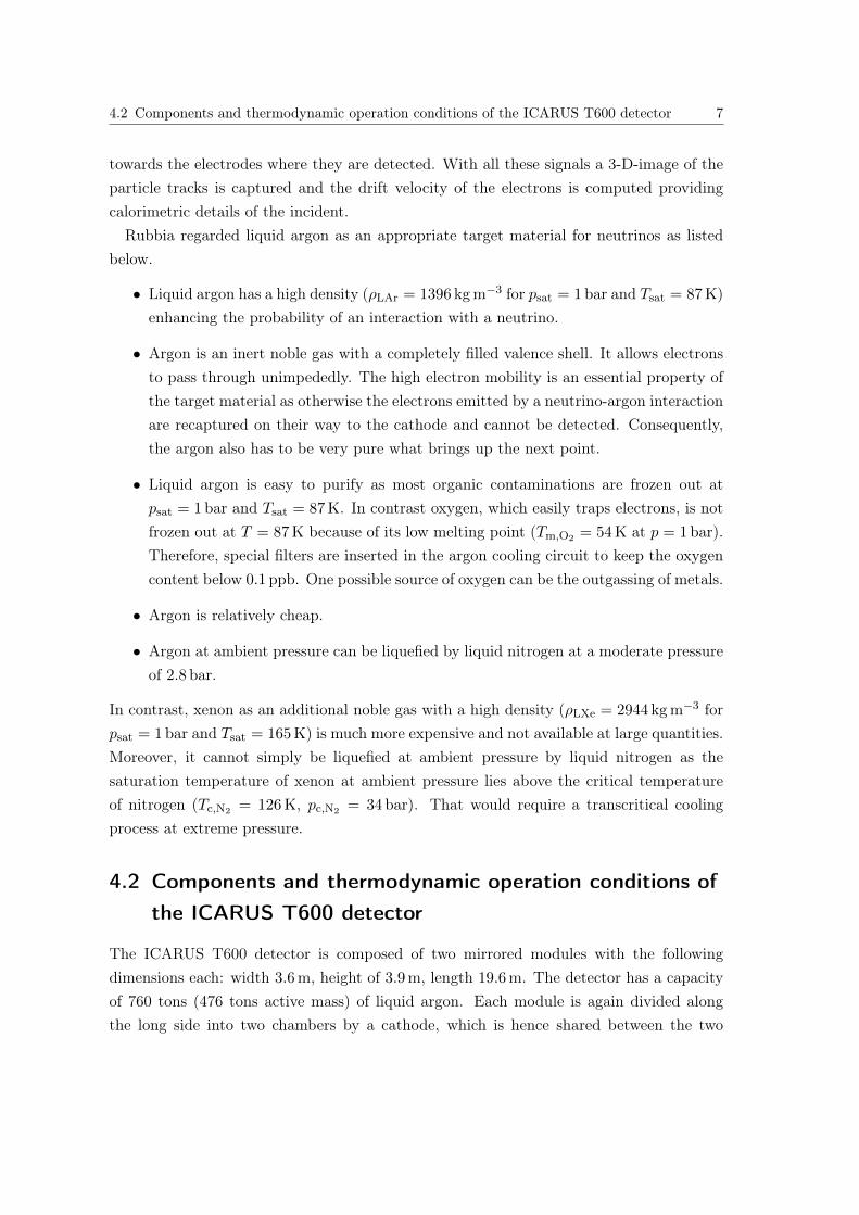
Fig. 4.1: Schematic of the ICARUS T600 detector [8].
chambers of one module. On the opposite side of the cathode all four chambers have ananode. This anode consists of around 54000 wires, which are arranged with a 3 mm pitch inthree different parallel planes at different angles of 0◦, ± 60◦. The created uniform electricfield has an intensity of 500 V m−1. The photomultipliers are mounted behind the anode[8]. Figure 4.1 illustrates the design of the ICARUS T600 detector.The whole ICARUS T600 detector is located inside a cryostat. Because of the detector’s
large size its operation is only feasible at ambient pressure. Thereby, the operation temper-ature of the detector is specified at 87.2 K, the saturation temperature of argon at ambientpressure. Due to safety reasons the pressure in the detector must be kept within a smallmargin of +20 mbarg and −5 mbarg. This implies a careful choice of the safety equipment.The pressure relief valves must have set points near ambient pressure, but should at thesame time be leak-tight. This pressure range corresponds, assuming saturation conditions,to an allowed temperature range of +187 mK and −48 mK. The liquid argon is cooledby boiling nitrogen as a coolant. The pressure of the nitrogen has to be kept at around2.8 bar. At ambient pressure the melting point of argon is with 83.8 K not much lowerthan the saturation temperature of 87.2 K. Freezing argon, meaning a pressure reduction
4.3 The thermal shield of the ICARUS T600 detector and its cooling concept 9
0
1
2
3
80 82 84 86 88 90
satu
ration p
ressure
in b
ar
temperature in K
argon
nitrogen
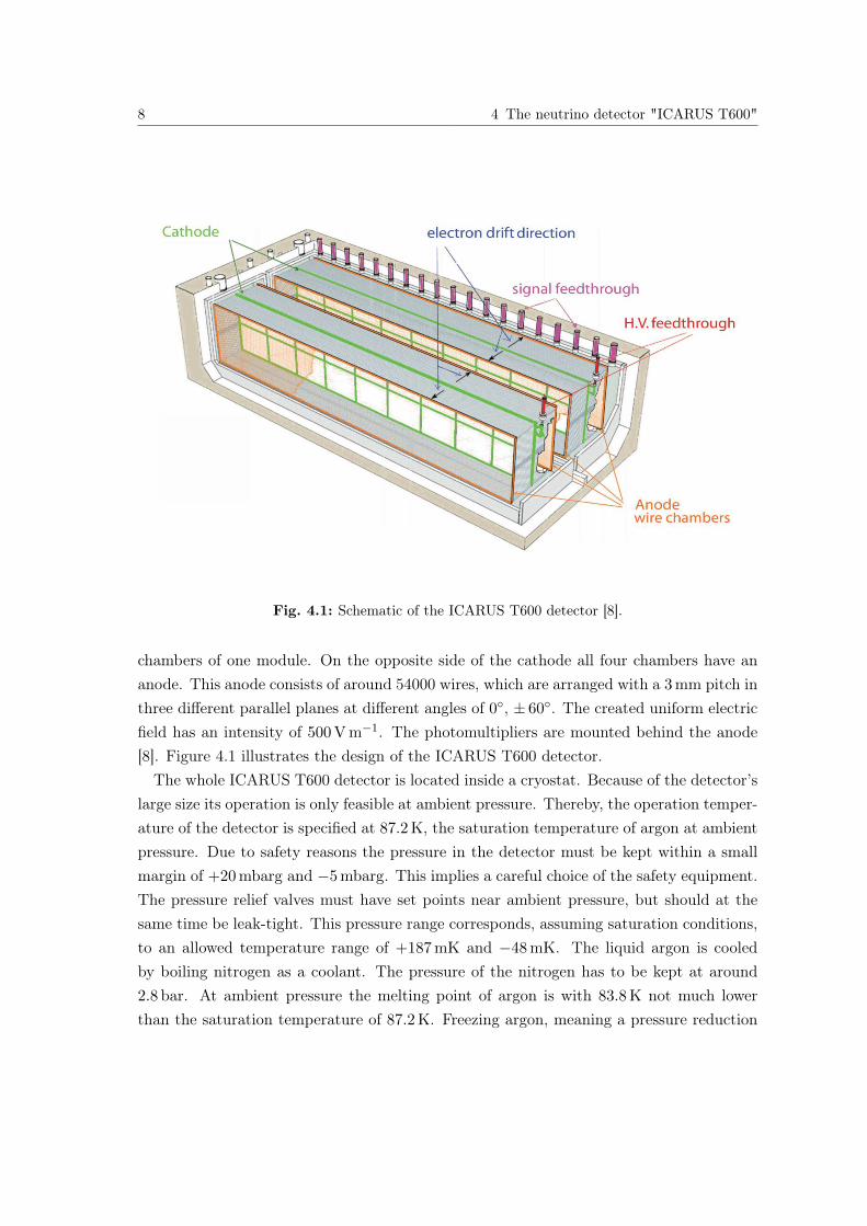
Fig. 4.2: Pressure-temperature-diagram with vapour pressure curves of argon and nitrogen. In-dicated are the maximal variations of the argon pressure (limits of the cryostat) and itsimplications for the stability of the nitrogen cooling loop around 2.8 bar.
of the cooling nitrogen system below approximately 2.04 bar, must be prevented under allcircumstances. Figure 4.2 shows the p-T-diagram with the vapour pressure curves of argon(in green) and nitrogen (in blue) highlighting the thermodynamic relations. The red lineshows the operation of the argon-boiling nitrogen cooling system at the nominal point of1 bar pressure. The black dashed lines indicate the small margin, in which the system hasto be stabilized. The red dotted line shows the conditions at the melting point of argon atambient pressure.
4.3 The thermal shield of the ICARUS T600 detector and itscooling concept
Owing to the strict constraints mentioned above it is crucial to properly insulate thecryostat against the environment diminishing the heat input from the outside. Liquid argonhas a low thermal conductivity (λLAr = 0.13 W m−1 K−1 at psat = 1 bar and Tsat = 87 K)
10 4 The neutrino detector "ICARUS T600"
enabling to maintain big temperature gradients in liquid argon, causing convection. Suchconvectional flow of liquid argon inside the detector should be prevented as it disturbs theprecise detection of the particle events. Because of the detector’s large size the vessel isnot vacuum-insulated but insulated by the help of an actively cooled thermal shield and a600 mm thick polyurethane foam insulation. It is important to emphasize that the coolingsystem of the thermal shield is independent from the main cooling system of the liquidargon.The Cryolab at CERN was assigned the task to support the design of the thermal
shield for the ICARUS T600 detector. The thermal shield is responsible of reducing theheat input from the surrounding environment into the cryostat and thus enables to keepthe liquid argon inside the detector within the required temperature range. The thermalshield should be at the same temperature of 87 K as the liquid argon inside the detectorto minimize the driving temperature gradient of the heat transfer. As coolant for thethermal shield nitrogen in the two-phase flow condition was chosen and the thermal shieldis kept at dry nitrogen gas atmosphere. Theoretically, not taking into account the pressuredrop, the nitrogen two phase flow can absorb a large amount of heat (∆hv = 185 kJ kg−1
at Tsat = 87 K) without changing temperature, as the temperature is constant duringevaporation. However, a pressure decrease due to a pressure drop along the thermal shieldalways corresponds to a temperature decrease in the two-phase area. The temperaturechange is normally much smaller than in single-phase flow, but has to be taken into accountdue to the strict temperature constraints of the thermal shield. To realize a saturationtemperature of 87 K the cooling system has to be operated at 2.8 bar. The thermal shieldshould meet the following conditions: It should be able to handle an outer heat flux densityof 20 W m−2 along one shield panel of approximately 11 m including the shield width. Atthe same time the maximum temperature gradient should be less than 500 mK. It shouldbe made by aluminium 1050A with a very high purity characterized by a low weightand a high thermal conductivity in comparison for example to ordinary steel (λAl1050A =
270 W m−1 K−1 at 87 K). By the help of an Ansys simulation as well as an experimentalsetup the thermal shield was designed as a combination of several panels. Each 4 mm thickpanel has a width of 472 mm. In the middle of each panel the pipe with an inner diameterof 10 mm is located (see figure 4.3). Each panel will be extruded with that geometry.The panels are assembled around the whole detector. There are 42 C-shaped panels atthe bottom and top as well as at the long side of each module of the detector and thereare 8 vertical panels at both frontal sides of each module. The manifold for the inlet ofthe nitrogen two-phase flow into each panel is between the two modules at the bottomof the detector and consequently the outlet is at the top. It is planned for the nitrogentwo-phase flow to have two horizontal flow sections and one vertical upward flow section,
4.3 The thermal shield of the ICARUS T600 detector and its cooling concept 11
Fig. 4.3: Drawing of one cooling panel stating the dimensions.
N2 inlet
N2 outlet
Fig. 4.4: Schematic of the cooling panels around the ICARUS T600 detector.
see picture 4.4. A mass flow of 2 g s−1 nitrogen in each panel is necessary to fulfil therequirements of a temperature gradient less than 500 mK, see Ansys simulation figure 4.5.The in total sixteen panels at the front and back side require a mass flow of 0.7 g s−1 each,as they are smaller. The total mass flow through the thermal shield is 179.2 g s−1. Theinlet flow quality is chosen to be 10 %.In a further step the pressure drop within the thermal shield, leading to a temperature
drop, should be investigated, which is the focus of the presented work.
12 4 The neutrino detector "ICARUS T600"
Fig. 4.5: Ansys simulation of the heat distribution in the cross-section of one cooling panel. Thetemperature rises from the middle of the panel towards the edges. Dark blue indicatesthe lowest temperature of 87 K and red indicates the highest temperature of 87.496 K,Courtesy D. Santandrea.
5 Nitrogen two-phase flow as refrigerantfor the cooling of the thermal shield
Two-phase flow describes the condition if a liquid and gaseous substance is flowing simulta-neously through a piping device. The gaseous substance can be the corresponding vapourto the liquid as well as another gas such as air. As in the case of nitrogen two-phase flowthe former is true, the gaseous substance is in the following always referred to as vapour.Two-phase flow is essentially different from single-phase flow because of the interactionbetween the two phases. Since the second half of the nineteenth century a lot of researchhas been performed in the field of two-phase flow [10]. A good introduction to two-phaseflow provide [11] and [12] and the content of this chapter is, unless otherwise specified,based on them.
5.1 Important characteristics of two-phase flow
The condition of two-phase flow is characterized by the following three important at-tributes: the flow quality, the flow pattern and the void fraction.
5.1.1 Flow quality
One characteristic parameter of two-phase flow is the flow quality x, see equation (5.1).The flow quality indicates the ratio of the mass flow of the vapour phase to the total massflow.
x =mv
ml + mv=
mv
mtot(5.1)
5.1.2 Flow pattern
However, the flow quality is not able to completely characterize the state of two-phase flow.The distribution of the two phases across the cross-sectional area of the pipe, the so-calledflow pattern, is essential for further analysis of the flow giving information about the extentof the phase boundary and the interaction of the two phases. Momentum exchange as wellas mass and heat transfer between the two phases, thus pressure drop and heat transfer
14 5 Nitrogen two-phase flow as refrigerant for the cooling of the thermal shield
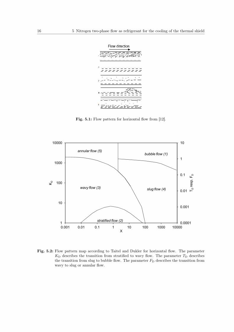
coefficients are influenced by the flow regime. In addition to the fluid properties the flowquality x and the mass flow density G are crucial to define the flow pattern. Moreover, theinteraction between the two phases is influenced by gravity and consequently by the angleof the pipe. In horizontal pipes the gravity works orthogonal to the flow direction, whereasin vertical pipes the gravity works in or against the flow direction. In the following, theflow pattern for horizontal and vertical pipes are described.For horizontal flow, the flow pattern map according to Taitel and Dukler [13] is recom-
mended in literature [11, 12, 14]. That flow pattern map of Taitel and Dukler is basedon an analytical theory, which predicts the transitions between the various flow regimes.The distribution of the two phases is determined by the balance of physical forces, mainlybuoyancy forces, surface forces and pressure differences. Figure 5.2 shows the flow patternmap according to Taitel and Dukler. Four different dimensionless quantities are used todefine the flow regime. On the x-axis the Lockart-Martinelli parameter X is plotted; theprimary vertical y-axis indicates the parameter KD and the secondary y-axis indicatesthe parameters TD or respectively FD. The parameter KD describes the transition fromstratified to wavy flow. It is dependent on the viscosity of the liquid phase because thewaves are formed by shear stress between the vapour and the liquid phase. The parameterTD describes the transition from slug to bubble flow. It considers the ratio between thefrictional pressure drop of the liquid phase if the liquid phase is assumed to flow alone inthe pipe and the buoyancy of the vapour phase. The parameter FD describes the transitionfrom wavy to slug or annular flow. It is dependent on the density ratio of both phasesand the Froude number, which is defined as the ratio of the flow inertia force to gravity.To define the flow pattern the following procedure has to be complied with. The limitingcurve between slug or wavy and annular flow is denoted as A(X). If FD(X) < A(X), drawKD versus X. If FD(X) ≥ A(X) as well as X ≤ 2 draw FD(X) versus X, otherwise drawTD versus X.
X =
(∆pl
∆pv
)0.5
(5.2)
KD =
(G3 · x2 · (1− x)
(ρl − ρv) · ρv · g · µl
)0.5
(5.3)
TD =
(∆pl∆L
(ρl − ρv) · g
)0.5
(5.4)
5.1 Important characteristics of two-phase flow 15
FD =G · x
((ρl − ρv) · ρv · g · d)0.5 (5.5)
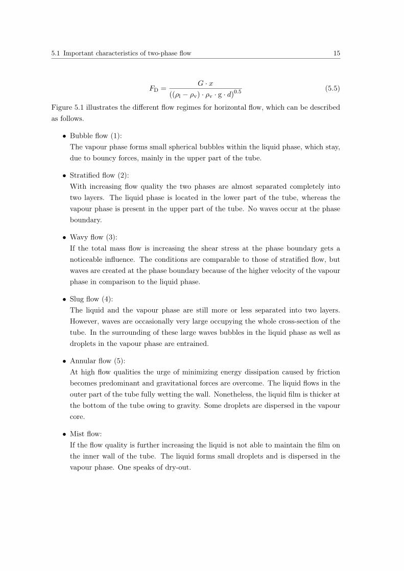
Figure 5.1 illustrates the different flow regimes for horizontal flow, which can be describedas follows.
• Bubble flow (1):The vapour phase forms small spherical bubbles within the liquid phase, which stay,due to bouncy forces, mainly in the upper part of the tube.
• Stratified flow (2):With increasing flow quality the two phases are almost separated completely intotwo layers. The liquid phase is located in the lower part of the tube, whereas thevapour phase is present in the upper part of the tube. No waves occur at the phaseboundary.
• Wavy flow (3):If the total mass flow is increasing the shear stress at the phase boundary gets anoticeable influence. The conditions are comparable to those of stratified flow, butwaves are created at the phase boundary because of the higher velocity of the vapourphase in comparison to the liquid phase.
• Slug flow (4):The liquid and the vapour phase are still more or less separated into two layers.However, waves are occasionally very large occupying the whole cross-section of thetube. In the surrounding of these large waves bubbles in the liquid phase as well asdroplets in the vapour phase are entrained.
• Annular flow (5):At high flow qualities the urge of minimizing energy dissipation caused by frictionbecomes predominant and gravitational forces are overcome. The liquid flows in theouter part of the tube fully wetting the wall. Nonetheless, the liquid film is thicker atthe bottom of the tube owing to gravity. Some droplets are dispersed in the vapourcore.
• Mist flow:If the flow quality is further increasing the liquid is not able to maintain the film onthe inner wall of the tube. The liquid forms small droplets and is dispersed in thevapour phase. One speaks of dry-out.
16 5 Nitrogen two-phase flow as refrigerant for the cooling of the thermal shield
Fig. 5.1: Flow pattern for horizontal flow from [12].
0.0001
0.001
0.01
0.1
1
10
1
10
100
1000
10000
0.001 0.01 0.1 1 10 100 1000 10000
TD
resp.
FD
KD
X
slug flow (4)
annular flow (5)bubble flow (1)
wavy flow (3)
stratified flow (2)
Fig. 5.2: Flow pattern map according to Taitel and Dukler for horizontal flow. The parameterKD describes the transition from stratified to wavy flow. The parameter TD describesthe transition from slug to bubble flow. The parameter FD describes the transition fromwavy to slug or annular flow.
5.1 Important characteristics of two-phase flow 17
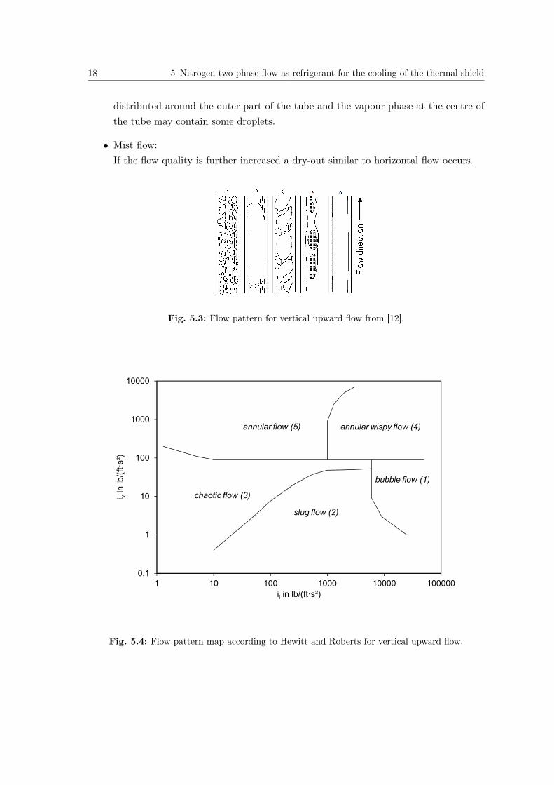
For vertical upward flow the flow pattern map according to Hewitt and Roberts [15]is recommended in literature [11, 12, 14]. That flow pattern map according to Hewittand Roberts is, in contrast to the flow pattern map of Taitel and Dukler, derived fromextensive experimental data. The flow pattern of different flows were visually observedby simultaneous x-ray and flash photography. Figure 5.4 shows the flow pattern mapaccording to Hewitt and Roberts. The momentum flux of the liquid as well as the vapourphase are plotted on the horizontal and vertical axis, see equation (5.6) and equation (5.7).In the original map the quantities are expressed in Imperial units.
il =(G · (1− x))2
ρl(5.6)
iv =(G · x)2
ρv(5.7)
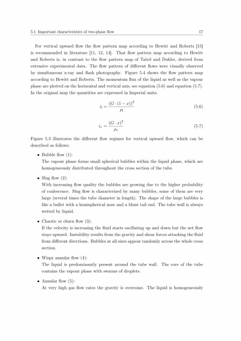
Figure 5.3 illustrates the different flow regimes for vertical upward flow, which can bedescribed as follows:
• Bubble flow (1):The vapour phase forms small spherical bubbles within the liquid phase, which arehomogeneously distributed throughout the cross section of the tube.
• Slug flow (2):With increasing flow quality the bubbles are growing due to the higher probabilityof coalescence. Slug flow is characterized by many bubbles, some of them are verylarge (several times the tube diameter in length). The shape of the large bubbles islike a bullet with a hemispherical nose and a blunt tail end. The tube wall is alwayswetted by liquid.
• Chaotic or churn flow (3):If the velocity is increasing the fluid starts oscillating up and down but the net flowstays upward. Instability results from the gravity and shear forces attacking the fluidfrom different directions. Bubbles at all sizes appear randomly across the whole crosssection.
• Wispy annular flow (4):The liquid is predominantly present around the tube wall. The core of the tubecontains the vapour phase with swarms of droplets.
• Annular flow (5):At very high gas flow rates the gravity is overcome. The liquid is homogeneously
18 5 Nitrogen two-phase flow as refrigerant for the cooling of the thermal shield
distributed around the outer part of the tube and the vapour phase at the centre ofthe tube may contain some droplets.
• Mist flow:If the flow quality is further increased a dry-out similar to horizontal flow occurs.
Fig. 5.3: Flow pattern for vertical upward flow from [12].
0.1
1
10
100
1000
10000
1 10 100 1000 10000 100000
i vin
lb/(
ft·s
²)
il in lb/(ft·s²)
annular flow (5) annular wispy flow (4)
chaotic flow (3)
slug flow (2)
bubble flow (1)
Fig. 5.4: Flow pattern map according to Hewitt and Roberts for vertical upward flow.
5.1 Important characteristics of two-phase flow 19
Recognized flow pattern maps for vertical downward flow doesn’t exist in literature.According to [14] the flow patterns for vertical downward flow are similar to those forvertical upward flow.It is important to note that all flow pattern maps mentioned above were developed for
adiabatic flow conditions. However, there exist also flow pattern maps for diabatic condi-tions such as the flow pattern map according to Kattan or Wojtan. The implementation ismuch more complex and big differences to the adiabatic flow pattern maps are only visibleat very high heat loads where the transition to mist flow and the prediction of the onsetof dry-out is of interest [16].
5.1.3 Void fraction
Another important characteristic of two-phase flow is the void fraction ε. That propertytakes into account that the two-phase flow is not uniform, but discontinuously fluctuating.Consequently, the local void fraction ε∗ at a specific location, see equation (5.8), shall varywith time. The function R equals one, if vapour is present and zero, if liquid is present.The variables x, y and z represent the three spatial dimensions. An average void fraction εcan be obtained by integrating the local void fraction ε∗, see equation (5.9). B representsa line, a surface or a volume.
ε∗ (x, y, z) =
∫R (x, y, z) dt∫
dt(5.8)
ε =
∫ε∗ (B) dB∫
dB(5.9)
The local void fraction ε∗ can be integrated over the volume of the tube leading toequation (5.10) by including the definition of the flow quality according to equation (5.1).
εvol =Vv
Vv + Vl
=
mvρv
mvρv
+ mlρl
=ρl · x
ρl · x+ (1− x) · ρv(5.10)
Usually, the local void fraction is integrated over the cross-sectional area of the tube yieldingto the equation (5.14). This equation is derived by coupling the equations of the velocityof the vapour phase, see equation (5.11), and the liquid phase, see equation (5.12), withthe slip factor S defined as the velocity ratio of the vapour phase to the liquid phase,see equation (5.13). The velocities of both phases can be expressed with the respectivemass flow through the part of the cross-sectional area that is occupied by the respectivephase. The rearranged equation (5.14), see equation (5.15), shows that normally the cross-
20 5 Nitrogen two-phase flow as refrigerant for the cooling of the thermal shield
sectional void fraction εcs is bigger than the flow quality x, as ρl ρ−1v � 1, and hence,
ρl ρ−1v S−1 > 1. Only at the critical point, where the density difference of the liquid and
vapour phase vanishes, the void fraction corresponds to the flow quality.
uv =mv
ρv ·A · εcs=
m · xρv ·A · εcs
(5.11)
ul =ml
ρl ·A · (1− εcs)=
m · (1− x)
ρl ·A · (1− εcs)(5.12)
S =uv
ul(5.13)
εcs =ρl · x
ρl · x+ (1− x) · ρv · S(5.14)
1
x− 1 =
(ρl
ρv
)· 1
S·(
1
εcs− 1
)(5.15)
The slip ratio S can be quantified by different correlations, over which Yu Xu et al.[17] gives a good overview. All these correlations are empirical and semi-empirical, as theunderlying detailed mechanism are still field of research. Nevertheless, Levy [18] and laterFujie [19] as well as Huq and Loth [20] developed some analytical correlations of the voidfraction.
1. Homogeneous correlation:The homogeneous correlation, not accounting for any interaction between the liquidand the vapour phase, assumes that both phases propagate at the same velocityand hence S = 1, compare equation (5.16). It is important to emphasize that thecross-sectional void fraction according to the homogeneous correlation correspondsto the volumetric void fraction in equation (5.10). It is only a function of the flowquality and the density of both phases εcs,hom = εvol = f (x, ρv(p, T ), ρl(p, T )). Thehomogeneous void fraction has a limited application range, favourable at conditionswhere the two phases move almost at the same velocity. That is the case for bubble ormist flow, where the dispersed phase has almost the same velocity as the continuousphase, and for high pressures near the critical pressure, where the density differencebetween the two phases vanishes.
εhom =ρl · x
ρl · x+ (1− x) · ρv(5.16)
5.1 Important characteristics of two-phase flow 21
2. Heterogeneous correlation:According to the heterogeneous correlation, accounting for the interaction betweenthe liquid and the vapour phase, the velocities of both phases are not similar and,hence, S 6= 1. The cross-sectional void fraction according to the heterogeneouscorrelation and the volumetric void fraction do not conform but are connected byequation (5.17). If S > 1, then εcs < εv applies, and if S < 1, then εcs > εv applies.In the following the cross-sectional void fraction εcs is always used and referred to byjust ε.
εvol =εcs
1S · (1− εcs) + εcs
⇐⇒ εcs =εvol
S · (1− εvol) + εvol(5.17)
The heterogeneous correlations can again be divided as follows:
a) K · εhom correlations:The simplest heterogeneous void fraction correlations are the K · εhom correla-tions. They are based on the homogeneous correlation multiplying the homoge-neous void fraction with a factor K. Referring to [17], the correlation accordingto Crisholm and the correlation according to Massena are the two correlationsof this category that predict best the reviewed literature data.
b) Slip ratio correlations:The slip ratio correlations express the slip ratio as a function of the flow qualityas well as fluid properties such as the density and the dynamic viscosity:
S = f
((1− xx
)p(ρv
ρl
)q ( µl
µv
)r). (5.18)
Referring to [17], the correlations according to Smith, Premoli et al. as well asOsmachkin and Borisov are the three correlations of this category that predictbest the reviewed literature data.
c) Drift-flux correlations:Drift flux correlations have the following form, see equation (5.19). The driftflux velocity uvj accounts for local phase velocity differences and is defined asthe velocity of the vapour with respect to the mixture. The parameter C0 takesinto account the effects of density and velocity distribution and is the ratioof the mean mixture volumetric flux to the area average volumetric flux. IfC0 = 1 the distribution is uniform, whereas if C0 6= 1 it is wide, more precisely,if C0 < 1 the vapour concentration at the wall is greater, and if C0 > 1, thevapour concentration in the core of the pipe is higher. The drift flux velocity uvj
22 5 Nitrogen two-phase flow as refrigerant for the cooling of the thermal shield
and the parameter C0 are subject to certain boundary conditions. If the voidfraction approaches zero and the liquid just starts boiling, the drift flux velocityuvj and the parameter C0 approaches zero assuming the bubbles be formed inthe boundary layer at the wall with an initial velocity of zero; or the drift fluxvelocity uvj and the parameter C0 are within their range when assuming thebubbles be formed in the fluid due to flashing. If the void fraction approachesone and the flow becomes all vapour the drift flux velocity vanishes and C0
becomes one. If the pressure approaches the critical pressure the flow becomeshomogeneous and uvj → 0 and C0 → 1, whereas if the pressure approaches zerouvj → ∞. In compliance with the mass conservation one obtains the followingequations for the velocity of the liquid, see equation (5.22), and vapour phase,see equation (5.21), enabling to calculate the slip ratio S [21, 22].
ε =Jv
C0 · J + uvjwith (5.19)
J = Jv + Jl =x ·Gρv
+(1− x) ·G
ρl(5.20)
uv =C0 ·G+ ρl · uvj
C0 · ε · ρv + (1− C0 · ε) · ρl(5.21)
ul =(1− C0 · ε) ·G− ε · ρv · uvj
(1− ε) [C0 · ε · ρv + (1− C0 · ε) · ρl](5.22)
Referring to [17], the correlation according to Rouhani or the correlation pro-posed by the authors themselves are the two correlations of this category thatpredict best the reviewed literature data. The original correlation according toRouhani [23] is based on the correlation according to Zuber and Findlay [24],but many different modifications of the Rouhani correlation exist in literature.In this work the version of the Rouhani correlation as defined in [17] is used.Especially for horizontal flow the correlation according to Steiner, a modifica-tion of the Rouhani correlation, is also frequently recommended in literature[11, 12, 25]. The correlation according to Chexal-Lellouche [21, 22, 26] includesall inclinations of the pipe.
5.1 Important characteristics of two-phase flow 23
d) Miscellaneous correlations:Miscellaneous other correlations can’t be classified in one of the four categoriesmentioned above. Many of them are using the Lockart-Martinelli parameter X.Referring to [17], the correlation according to Yashar et al. and the correlationaccording to Huq and Loth are the two correlations of this category that predictbest the reviewed literature data.
Heterogeneous correlations, by factoring in the interaction between the vapour and theliquid phase, reflect the dependency of the void fraction on the flow pattern, thus, themass velocity and the flow direction. By referring to equation (5.14) the following generalconclusion can be drawn. If the vapour phase flows faster than the liquid (S > 1), normallythe case for vertical upward and horizontal flow, the homogeneous void fraction εhom isthe upper threshold for the void fraction. If the velocity of the liquid phase exceeds thevelocity of the vapour phase (S < 1), potentially the case for vertical downward flow due togravity effects, the homogeneous void fraction is the lower threshold for the void fraction.In the following the focus is on selected void fraction correlations: the homogeneous
void fraction, the correlation according to Crisholm as K · εhom correlation and the drift-flux correlations according to Rouhani, Steiner and Chexal-Lellouche. Figure 5.5 showsthe void fraction according to these correlations versus the flow quality and figure 5.6shows the dependency of the void fraction on the mass flow. Both figures are calculatedfor nitrogen two-phase flow at the saturation conditions of psat = 1 bar and Tsat = 87 K.Figure 5.5 shows the dependency of the void fraction on the flow direction. In general,the void fraction increases with increasing flow quality. The slope is larger at low flowqualities. The void fraction correlation according to Rouhani as defined in [17] (referred toas Rouhani I) violates the boundary condition of ε = 1 at x = 1 and, hence, fails to predictthe void fraction at high flow qualities. The version of the Rouhani correlation according to[27] would solve this problem. Comparing Steiner and Rouhani, the void fraction of Steiner(horizontal flow) is over the whole range of the flow quality greater than the void fraction ofRouhani, preferable used for vertical upward flow. That corresponds to the description ofthe previous paragraph. On the contrary, according to Chexal-Lellouche, the void fractionfor horizontal flow lies only above the void fraction for vertical upward flow for flow qualitiessmaller than 25 %. The correlation according to Chexal-Lellouche for vertical downwardflow and the heterogeneous correlation predict the highest void fractions. Figure 5.6 reflectsthe fact, that the void fraction increases with increasing mass velocity [28]. Of course, thehomogeneous correlation as well as the correlation according to Crisholm don’t take thisphenomena into account. However, the correlation according to Chexal and Lellouchepredicts a moderate increase of the void fraction, whereas Rouhani and Steiner predict asharper rise of the void fraction with growing mass velocity. Moreover, as most of these
24 5 Nitrogen two-phase flow as refrigerant for the cooling of the thermal shield
0
0.2
0.4
0.6
0.8
1
0 0.2 0.4 0.6 0.8 1
void
frac
tion
flow quality
homogeneous modelCrisholmChexal/Lellouche (downward)SteinerChexal/Lellouche (horizontal)Rouhani IRouhani IIChexal/Lellouche (upward)
Fig. 5.5: Void fraction according to different correlations versus flow quality for a mass veloc-ity of 25.5 kg m−2 s−1, calculated for nitrogen two-phase flow at saturation conditionspsat = 1 bar and Tsat = 87 K. Only the correlation according to Chexal-Lellouche distin-guishes between different inclinations of the pipe. The correlation of Rouhani is oftenrecommended in literature for vertical upward flow. The correlation of Steiner is oftenrecommended in literature for horizontal flow. For the correlation of Crisholm the angleof the pipe is not specified.
void fraction correlations are derived from experiments conducted with water and steam,water and air or refrigerants like R134a, it cannot be concluded automatically that theyare also applicable for nitrogen. One special feature of nitrogen is its low density ratio ofthe liquid to the vapour phase in comparison with customary refrigerants and particularlywater (ρN2,l ρ
−1N2,v
= 65 at psat = 1 bar and Tsat = 87 K). Thus, owing to the lack ofcorrelations for nitrogen two-phase flow, the experimental small-scale measurement setupbuilt up in the Cryolab enables an interesting study, which will contribute to extend thegeneral knowledge of the refrigerant nitrogen used in several different applications, such asthe ICARUS detector’s thermal shield.
5.2 Pressure drop in two-phase flow 25
0
0,2
0,4
0,6
0,8
1
10 20 30 40 50
void
fra
ction
mass velocity in kg/(m2·s)
homogeneous model
Crisholm
Chexal/Lellouche (downward)
Steiner
Chexal/Lellouche (horizontal)
Rouhani I
Rouhani II
Chexal/Lellouche (upward)
Fig. 5.6: Void fraction according to different correlations versus mass velocity for a flow qualityof 10 %, calculated for nitrogen two-phase flow at saturation conditions psat = 1 bar andTsat = 87 K . Only the correlation according to Chexal-Lellouche distinguishes betweendifferent inclinations of the pipe. The correlation of Rouhani is often recommended inliterature for vertical upward flow. The correlation of Steiner is often recommended inliterature for horizontal flow. For the correlation of Crisholm the angle of the pipe isnot specified.
5.2 Pressure drop in two-phase flow
The total pressure drop of two-phase flow along a pipe is the sum of the gravitational,frictional and momentum pressure drop:
∆p = ∆pg + ∆pf + ∆pmom . (5.23)
5.2.1 Gravitational pressure drop in two-phase flow
The gravitational pressure drop is calculated, in analogy to single-phase flow, by the fol-lowing equation:
∆pg = ρ2ph · g · sin(ϕ) · L . (5.24)
26 5 Nitrogen two-phase flow as refrigerant for the cooling of the thermal shield
The two-phase density ρ2ph is defined according to equation (5.25). If the homogeneousvoid fraction εhom, see equation (5.16), is used, the equation for the two-phase densitysimplifies to equation (5.26). As can be seen in figure 5.5, the void fraction according tovarious heterogeneous correlations is always smaller than the homogeneous void fraction,except for vertical downward flow. Consequently, the two-phase density calculated withthe heterogeneous void fraction is higher than the homogeneous two-phase density, exceptfor vertical downward flow, where it is the other way around.
ρ2ph = (1− ε) · ρl + ε · ρv (5.25)
ρ2ph,hom =ρl · ρv
ρl · x+ ρv · (1− x)(5.26)
The gravitational pressure drop only affects the total pressure drop if the pipe is nothorizontal. In literature it is still discussed if for two-phase vertical downward flow thegravitational pressure drop results in a pressure gain, as well-known from single-phaseflow, or if the pressure gain is negligible due to the buoyancy forces of the vapour [10].
5.2.2 Frictional pressure drop in two-phase flow
The frictional pressure drop accounts for the friction caused by wall roughness as wellas interfacial roughness. It is calculated according to empirical or semi-empirical models,which are based on the well-known single-phase frictional pressure drop. The frictionfactor is normally independent of the wall roughness as the two-phase flow interactioneffects prevail over the effects of the wall roughness [29].
∆p = f · Ld· 0.5 · ρ · u2 = f · L
d· 0.5 · G
2
ρwith (5.27)
f = f(Re), Re =G · dµ
(5.28)
The models can be categorised as follows [30]:
1. Homogeneous models:The two-phase frictional pressure drop is calculated by the universal equation (5.27)using the total mass velocity and two-phase properties averaged between the vapourand liquid properties. The models differ in determining the two-phase properties.According to [30], the models of Beattie-Whalley, McAdams et al. and Cicchitti et al.are the homogeneous models that predict best the reviewed literature data.
5.2 Pressure drop in two-phase flow 27
2. Separated flow models:Separated flow models obtain the two-phase frictional pressure drop by multiplyingthe single-phase frictional pressure drop (liquid or vapour phase) by a two-phasemultiplier φ2, see equation (5.29). Separated flow models allow, by defining differ-ent case-dependent two-phase multipliers, to consider that the two-phase frictionalpressure drop is influenced by the flow pattern, hence varying with the flow direc-tion and the flow regime. However, only some pressure drop models like [16, 25] areflow-pattern based. As proofed in literature and previous measurements of two-phasepressure drop of carbon dioxide at CERN demonstrated, the heat input has no or athigh heat inputs of several kW m−2 only marginal impact on the frictional pressuredrop [31, 32]. (
∆p
∆L
)2ph
=
(∆p
∆L
)l
· φ2l =
(∆p
∆L
)v
· φ2v (5.29)
a) φ2l , φ
2v - method:
The φ2l , φ
2v - method determines the single-phase pressure drop of the vapour
and the liquid phase assuming that the respective flow propagates alone in thepipe. Well-known representative of this kind of model is the model according toLockart and Martinelli. According to [30], only the model of Sun and Mishimapredicts the reviewed literature data with a sufficient accuracy.(
∆p
∆L
)l
= fl(G(1− x))2
2 · d · ρl,(
∆p
∆L
)v
= fv(G · x)2
2 · d · ρv(5.30)
b) φ2l0, φ
2v0 - method:
The φ2l0, φ
2v0 - method determines the single-phase pressure drop of the vapour
and the liquid phase assuming that the total flow is in the respective state.Well-known representatives of this kind of model are the models according toFriedel [33], Müller-Steinhagen and Heck [34], Gronnerud [35] and Crisholm.According to [30], the models of Souza and Pimenta and Cavallini also pre-dict the reviewed literature data with a sufficient accuracy. Only the model ofMüller-Steinhagen and Heck has been developed by pressure drop measurementsof, amongst others, nitrogen.(
∆p
∆L
)l
= fl0G2
2 · d · ρl,(
∆p
∆L
)v
= fv0G2
2 · d · ρv(5.31)
The frictional pressure drop plotted versus the flow quality shows a characteristic curvewith a maximum of the pressure drop at a flow quality of approximately 80 % or slightly
28 5 Nitrogen two-phase flow as refrigerant for the cooling of the thermal shield
0
0.4
0.8
1.2
1.6
0 0.2 0.4 0.6 0.8 1
pre
ssure
dro
p p
er
length
in m
bar/
m
flow quality
Friedel (horizontal and vertical upward flow)
Friedel (vertical downward flow)
Müller-Steinhagen and Heck
Gronnerud
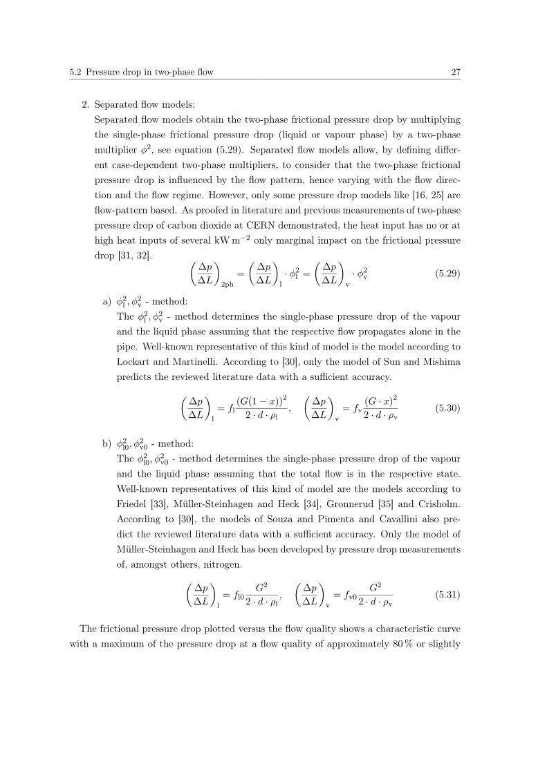
Fig. 5.7: Frictional pressure drop according to different models versus flow quality for a mass flowof 2 g s−1 in a pipe with an inner diameter of 10 mm , calculated for nitrogen two-phaseflow at saturation conditions psat = 1 bar and Tsat = 87 K. Only the model according toFriedel distinguishes between the inclination of the pipe.
above. After passing through the maximum the frictional pressure drop decreases to thefrictional pressure drop of single-phase vapour flow. Figure 5.7 shows the course of the two-phase frictional pressure drop calculated by selected models according to Friedel, Müller-Steinhagen and Heck as well as Gronnerud versus the flow quality for the conditions in theICARUS detector’s thermal shield (nitrogen flow at saturation conditions of psat = 1 bar
and Tsat = 87 K). The model of Friedel proposes two different models, one for horizontaland vertical upward flow and the other for vertical downward flow. The frictional pressuredrop in the latter case is higher as gravity and the buoyancy forces counteract. Thefrictional pressure drop model according to Friedel is the most conservative one at existingconditions.
5.2 Pressure drop in two-phase flow 29
5.2.3 Momentum pressure drop in two-phase flow
Unlike single-phase flow, the momentum pressure drop has to be factored in the totalpressure drop for two-phase flow. It accounts for the pressure drop owing to the accelerationof molecules during the evaporation process, as molecules from the slower liquid phase enterthe faster vapour phase.
∆pmom = G2
{((1− x)2
(1− ε) · ρl+
x2
ε · ρv
)out
−(
(1− x)2
(1− ε) · ρl+
x2
ε · ρv
)in
}(5.32)
In general, the momentum pressure drop is higher at low flow qualities as the change of thevoid fraction at low flow qualities is more distinct. The absolute value of the momentumpressure drop can be several orders of magnitude smaller than the absolute value of thegravitational as well as frictional pressure drop. When the difference of the flow qualities atthe inlet and outlet is large, particularly the case in non-adiabatic flow, or if the differenceof the densities between the vapour and the liquid phase is huge, especially true at lowsystem pressure, the momentum pressure drop can have a considerable contribution to theoverall pressure drop.
6 Numeric model for nitrogen two-phaseflow pressure drop
The numerical program described in this chapter calculates the two-phase pressure dropand has been developed for nitrogen two-phase flow at saturation conditions close to psat =
2.8 bar and Tsat = 87 K. Different correlations for the void fraction as well as for thefrictional pressure drop of two-phase flow can be integrated into the program by embeddingdifferent subfunctions into the main program. A measurement campaign is planned tovalidate the program and to allow to chose the void fraction and frictional pressure dropcorrelations from the literature, that describe best nitrogen two-phase flow at conditionssimilar to those of the ICARUS detector’s thermal shield. Subsequently, if the program isable to reproduce the measurement data with a satisfying accuracy, the overall pressuredrop over the real large-scale ICARUS thermal shield can be computed and the final designcan be defined.The mathematical description for the two-phase pressure drop has been implemented inMatlab R©. The flow chart in the appendix B illustrates the simplified program structure.First of all, the user has to specify the following input parameters: pipe dimensions (innerdiameter, length and orientation), the flow conditions (mass flow and heat flux), andthe inlet conditions (saturation pressure and either enthalpy or flow quality). The exactfluid properties of nitrogen (saturation temperature and enthalpies, densities, viscositiesof both phases as well as surface tension of liquid phase) at saturation pressures in therange of 2.6 bar to 2.9 bar are calculated with the embedded function "fluid properties".The function comprises the corresponding fit functions of NIST data. Knowing the fluidproperties, the enthalpy or the flow quality (the quantity which has not been defined beforeby the user) can be calculated as well as the void fraction and the average density. Theinlet conditions are referred to as "0" and the pressure drops at the pipe inlet are set tozero. The length of the pipe is discretizised in N 1 mm long parts. The outlet conditions ofthe previous part are the inlet conditions of the subsequent part, numerically realized bya for-loop. In each loop run the new outlet enthalpy of the part is determined accordingto the first law of thermodynamics, see equation (6.2). Equation (6.2) is derived fromequation (6.1), which represents the one-dimensional energy equation for a steady-state
31
open system with one material flow. The program assumes a homogeneous distribution ofthe heat load over the length of the pipe, that means, each part has a heat load of Q/N .Based on the outlet enthalpy other important characteristics of the flow (flow quality, voidfraction, average density) can be computed, which are then used to finally determine themomentum, gravitational, frictional and total pressure drop over the part. An iterativecomputation is necessary as the outlet enthalpy is, among other variables, a function ofthe outlet fluid properties, which correspond to the a priori unknown outlet saturationpressure. Consequently, as a first step, the outlet fluid properties are approximated bythe inlet values, and their real values and the exact pressure drop are then approachedby an iteration, numerically realized by a do-while-loop. The do-while-loop is abortedif the difference of the outlet pressure calculated in the current loop run and the onecalculated in the previous loop run is smaller than 10−7 bar. As mentioned above, differentcorrelations for the void fraction and the frictional pressure drop can be included in theprogram. If the pipe has several sections with different orientations, the calculation has tobe done sectionwise, with outlet values of the previous section being the inlet values of thesubsequent section. In the following, the following naming convention is used: programrefers to the Matlab R© program, correlation refers to the void fraction correlation for two-phase flow and model refers to the frictional pressure drop model for two-phase flow.
Q+@@P = m
[(h+
u2
2+ gz
)out
−(h+
u2
2+ gz
)in
](6.1)
hout = hin +Q
m− 0.5 ·G2
(1
ρ2out
− 1
ρ2in
)− g · (zout − zin) (6.2)
7 Small-scale setup for nitrogentwo-phase flow pressure dropmeasurements
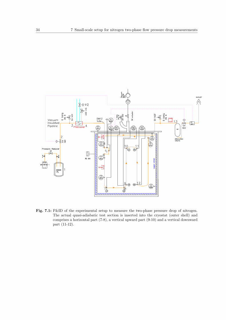
A small-scale experimental setup has been built in the Cryolab to measure the pressuredrop of nitrogen two-phase flow at saturation conditions of psat = 2.8 bar and Tsat = 87 K.The pressure drop has been determined in a quasi-adiabatic test section, comprising ahorizontal, vertical upward and downward part, varying the mass flow and the flow quality.
7.1 Design and instrumentation of the experimental setup
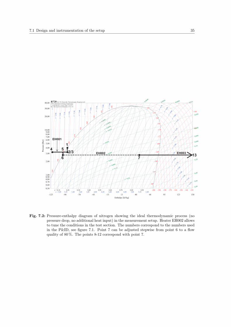
Figure 7.1 shows the piping and instrumentation diagram (P&ID) of the small-scale exper-imental setup and figure 7.2 illustrates the ideal thermodynamic process (no pressure drop,no additional heat load) of the measurement in the p-h diagram. The setup has mostlybeen taken over from a previous one, which has been designed to perform a measurementcampaign aiming to determine the temperature profile of the ICARUS detector’s thermalshield in order to validate the ANSYS simulation shown in figure 4.5. The setup hasbeen modified and substantially upgraded to measure the pressure drop in three differentoriented pipe sections. Liquid nitrogen is supplied from a 500 l Dewar. The subsequentprecooler filled with liquid nitrogen is operated at ambient pressure and allows to subcoolthe nitrogen flow. Theoretically, assuming an infinite heat transfer surface, the nitrogenflow could be cooled down to 78 K, the saturation temperature of nitrogen at ambientpressure. However, in practice, a finite heat transfer surface and heat load of the connec-tion pipes and feedthroughs cease the nitrogen flow to a temperature between 82 K and85 K depending on the total mass flow. Heater EH001 allows to adjust the initial pointfor the isenthalpic Joule-Thomson expansion, realized by a needle valve, so that the flowquality after the expansion into the two-phase area is around 1 − 2 %. The two-phasearea is entered by an expansion and not by heating in order to prevent instabilities ofthe system due to boiling delay effects. The thermodynamic equilibrium is assumed to bereached instantaneously. The heater EH003 after the test section fully evaporates the flow,so that the mass flow can be determined by a Venturi flowmeter at ambient temperature
7.1 Design and instrumentation of the setup 33
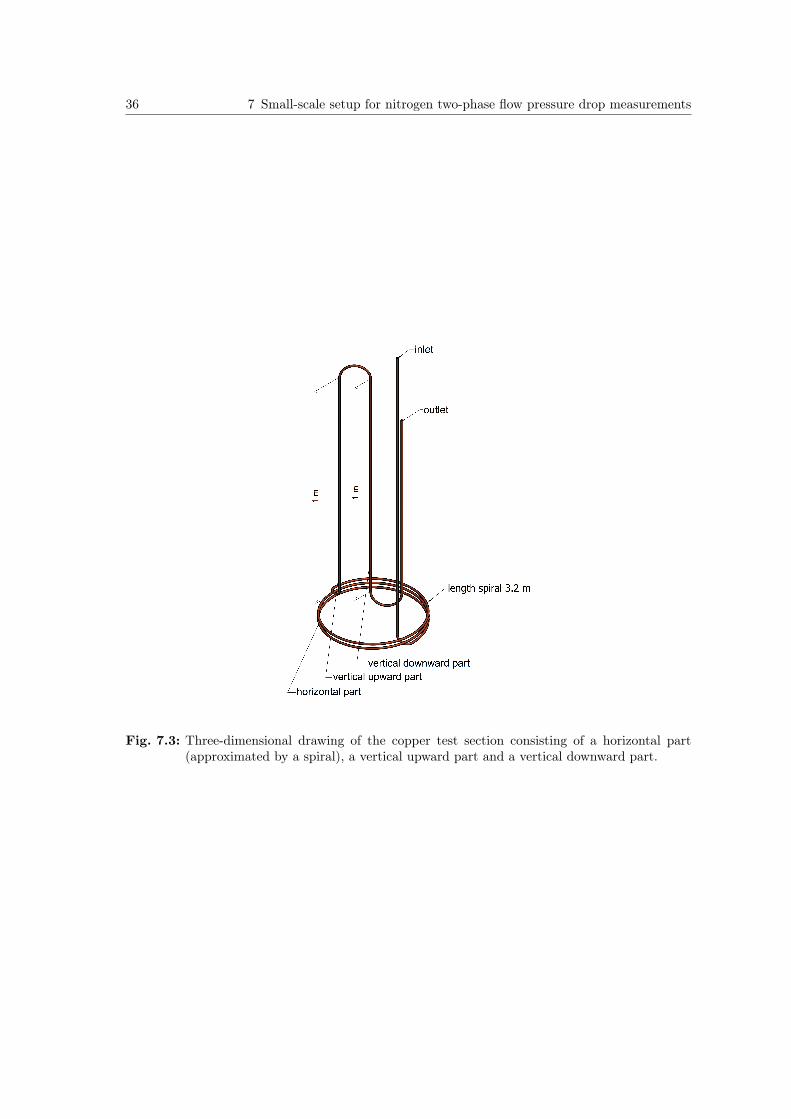
conditions. The cartridge heater EH002 shall tune the flow quality for the real test section.A detailed drawing of the cartridge heater device can be found in the appendix A. It hasbeen designed with an annular gap of 1 mm representing an optimum between pressuredrop and heat transfer. The test section is made out of a copper tube with an inner diam-eter of 6 mm. Its geometry is depicted in figure 7.3. It consists of a horizontal part with alength of 3.2 m, a vertical upward part and a vertical downward part with a length of 1 m
each. The horizontal part of the test section is approximated by a spiral due to limitedspace inside the cryostat. The curvature radius of the spiral is so large, that it should notaffect the pressure drop of the nitrogen flow. To guarantee quasi-adiabatic conditions ofthe test section the following technically feasible solutions were implemented. Firstly, MLI(multi-layer insulation) is put around the sample. Secondly, a thermal shield, externallycovered with MLI, is mounted around the sample. Thirdly, the lowest top plate of theinsert is actively cooled by means of the sample outlet nitrogen flow and also cools thelinked shield. All three above mentioned measures reduce the heat input by radiation intothe test section. Finally, the whole cryostat is set to a vacuum pressure of 10−4 mbar
before cool down to diminish heat transfer by convection. The special pressure tab deviceaverages the pressure drop over the pipe cross-section by means of four evenly distributedholes, shown in the appendix A. At the beginning of the capillaries, connecting the pressuretab devices with the pressure sensors at the top of the cryostat, little heaters (H1-H6) areattached to ensure that there is no liquid column in the capillaries distorting the pressuredrop measurements. The pressure in the test section is measured by pressure sensor PTN03and regulated with outlet valve CVN02. The attenuation volume (AV) helps to stabilizethe pressure inside the test section. The mass flow in the test section is measured by theVenturi flowmeter and is regulated with inlet valve CVN01. The pressure and mass flowcontrol is further discussed in section 8.3.
34 7 Small-scale setup for nitrogen two-phase flow pressure drop measurements
Fig. 7.1: P&ID of the experimental setup to measure the two-phase pressure drop of nitrogen.The actual quasi-adiabatic test section is inserted into the cryostat (outer shell) andcomprises a horizontal part (7-8), a vertical upward part (9-10) and a vertical downwardpart (11-12).
7.1 Design and instrumentation of the setup 35
���������� ���
���� ��� ��� ��� ��� �� �� �� �� ��� ���
�������� ���
�!��
�!��
�!��
�!���!���!���!��
�!��
�!��
�!��
�!��
�!��
�!��
�!���!����!��
��!��
��!��
��!��
�"�!��
�"�!��
�"�!��
�"�!��
�"�!��
�"�!��
�"�!��
�"�!��
�"�!��
�"�!��
�"�!��
�"�!��
�"�!��
�"�!��
�"�!��
�"�!��
�"�!��
�"�!��
�" �!��
�"�! ��
�"�!��
�"�!��
�"�!��
�"�!��
�"�!��
�"�!��
�"�!��
�"�!��
����
����
����
����
����
����
����
����
����
����
����
����
����
����
����
����
����
���� ����
����
����
����
����
����
����
����
����
����
����
����
����
�!����
�!����
�!����
�!���
�!���
�!���
�!���
�!���
�!��
�!��
�!��
�!��
�!��
#"�!�� �!�� �!�� �!�� �!�� �!�� �!�� �!�� �!���"�!�� �!�� �!�� �!�� �!�� �!�� �!�� �!�� �!�� �!�� �!�� �!�� �!��
$"�!����
$"�!�
���
$"�!�
���
$"�!���
$"�!���
$"�!���
$"�!���
$"�!���
$"�!��
$"�!��
%&'!%�����(���)*���������+����+��
�+��� ,��-.�/$+�(0� ���/&+�12�
3/�/4�)$���56/�/6-��7���/��������
���� 8�*9:/2/8���)�7�9&���()7���(+;��)����+��+�4<
4
EH001
5
1
2/3
6
EH002 EH00313
7
Fig. 7.2: Pressure-enthalpy diagram of nitrogen showing the ideal thermodynamic process (nopressure drop, no additional heat input) in the measurement setup. Heater EH002 allowsto tune the conditions in the test section. The numbers correspond to the numbers usedin the P&ID, see figure 7.1. Point 7 can be adjusted stepwise from point 6 to a flowquality of 80%. The points 8-12 correspond with point 7.
36 7 Small-scale setup for nitrogen two-phase flow pressure drop measurements
Fig. 7.3: Three-dimensional drawing of the copper test section consisting of a horizontal part(approximated by a spiral), a vertical upward part and a vertical downward part.
7.2 Uncertainty of the two-phase flow pressure drop measurements 37
7.2 Uncertainty of the two-phase flow pressure dropmeasurements
The uncertainty of the measurement has been evaluated by the following method, whichestimates the maximum error and specifies a range, in which the true value is allocated. Ithas to be noted that systematic errors are not included in this measurement uncertaintyevaluation. Assuming that the value A is calculated from the values Z1 to Zn, which aredirectly measured, then the maximum error of the value A is determined by equation (7.1).The errors of the single values ∆Z1 to ∆Zn are obtained by the measuring instrumentsaccuracy specified by the manufacturer plus the noise of the measurement signal, which iscalculated by the standard deviation of the signal. As the signal noise is high comparedto the reference accuracies, due to the instabilities in two-phase flow, and it is the onlystatistical error, the signal noise is added to the accuracies to determine the maximumerror.
∆A =n∑1
∣∣∣∣ ∂A∂Zn·∆Zn
∣∣∣∣ (7.1)
The following measuring instruments have been used.
• WIKA absolute pressure transmitter: model S-10 [A]
• ROUSEMOUNT differential pressure transmitter: model 3051C [B]
• KEITHLEY DMM multimeter: 199 System DMM Scanner [C]
• FLUKE PHILIPS system multimeter: PM 2534 [D]
• NATIONAL INSTRUMENTS PXI: NI PXI 8115 [E]
Table 7.1 gives an overview of the accuracies of the used measuring instruments accordingto the manufacturers. If data for the temperature effect, the pressure effect and the long-term stability exists, it is included in table 7.1. As all measuring instruments have beencalibrated at known calibration points at the beginning of the measurement campaign, atime period of one year is assumed for the long-term stability. The temperature differencein the Cryolab is assumed to be a maximum of 5 K.
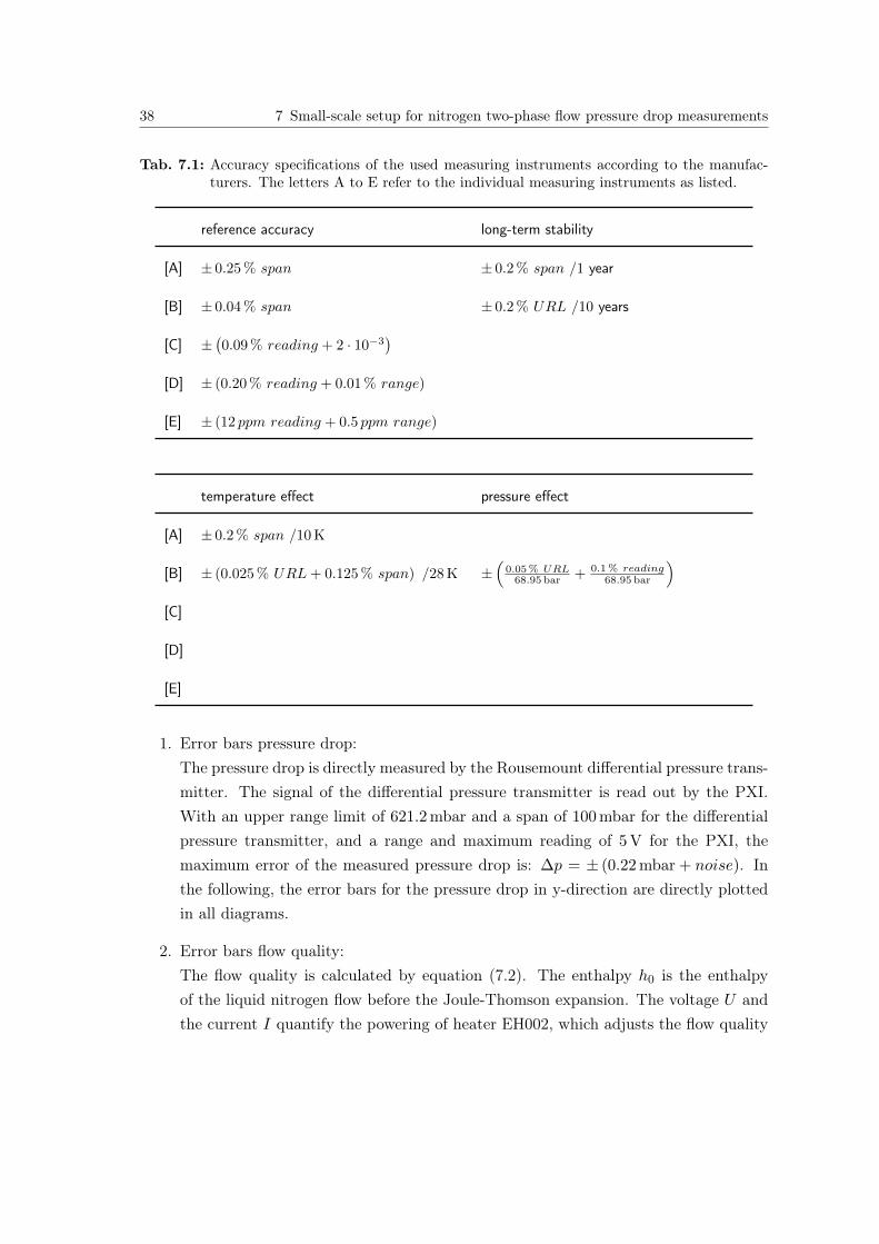
38 7 Small-scale setup for nitrogen two-phase flow pressure drop measurements
Tab. 7.1: Accuracy specifications of the used measuring instruments according to the manufac-turers. The letters A to E refer to the individual measuring instruments as listed.
reference accuracy long-term stability
[A] ± 0.25 % span ± 0.2 % span /1 year
[B] ± 0.04 % span ± 0.2 % URL /10 years
[C] ±(0.09 % reading + 2 · 10−3
)[D] ± (0.20 % reading + 0.01 % range)
[E] ± (12 ppm reading + 0.5 ppm range)
temperature effect pressure effect
[A] ± 0.2 % span /10 K
[B] ± (0.025 % URL+ 0.125 % span) /28 K ±(
0.05% URL68.95 bar + 0.1% reading
68.95 bar
)[C]
[D]
[E]
1. Error bars pressure drop:The pressure drop is directly measured by the Rousemount differential pressure trans-mitter. The signal of the differential pressure transmitter is read out by the PXI.With an upper range limit of 621.2 mbar and a span of 100 mbar for the differentialpressure transmitter, and a range and maximum reading of 5 V for the PXI, themaximum error of the measured pressure drop is: ∆p = ± (0.22 mbar + noise). Inthe following, the error bars for the pressure drop in y-direction are directly plottedin all diagrams.
2. Error bars flow quality:The flow quality is calculated by equation (7.2). The enthalpy h0 is the enthalpyof the liquid nitrogen flow before the Joule-Thomson expansion. The voltage U andthe current I quantify the powering of heater EH002, which adjusts the flow quality
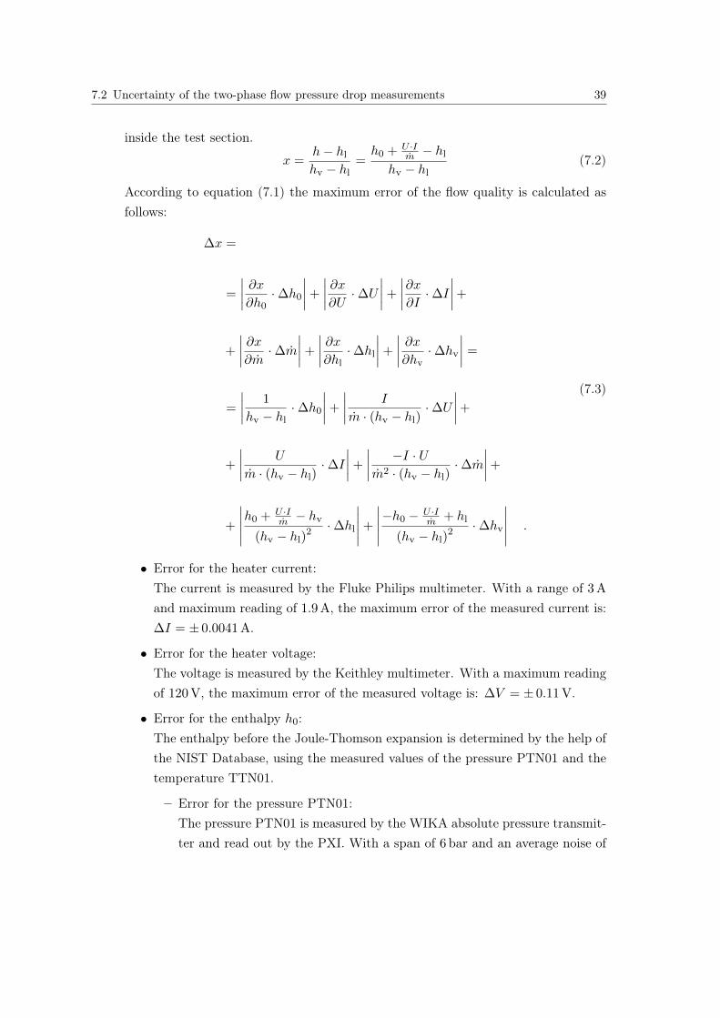
7.2 Uncertainty of the two-phase flow pressure drop measurements 39
inside the test section.
x =h− hl
hv − hl=h0 + U ·I
m − hl
hv − hl(7.2)
According to equation (7.1) the maximum error of the flow quality is calculated asfollows:
∆x =
=
∣∣∣∣ ∂x∂h0·∆h0
∣∣∣∣+
∣∣∣∣ ∂x∂U ·∆U∣∣∣∣+
∣∣∣∣∂x∂I ·∆I∣∣∣∣+
+
∣∣∣∣ ∂x∂m ·∆m∣∣∣∣+
∣∣∣∣ ∂x∂hl·∆hl
∣∣∣∣+
∣∣∣∣ ∂x∂hv·∆hv
∣∣∣∣ =
=
∣∣∣∣ 1
hv − hl·∆h0
∣∣∣∣+
∣∣∣∣ I
m · (hv − hl)·∆U
∣∣∣∣++
∣∣∣∣ U
m · (hv − hl)·∆I
∣∣∣∣+
∣∣∣∣ −I · Um2 · (hv − hl)
·∆m∣∣∣∣+
+
∣∣∣∣∣h0 + U ·Im − hv
(hv − hl)2 ·∆hl
∣∣∣∣∣+
∣∣∣∣∣−h0 − U ·Im + hl
(hv − hl)2 ·∆hv
∣∣∣∣∣ .
(7.3)
• Error for the heater current:The current is measured by the Fluke Philips multimeter. With a range of 3 A
and maximum reading of 1.9 A, the maximum error of the measured current is:∆I = ± 0.0041 A.
• Error for the heater voltage:The voltage is measured by the Keithley multimeter. With a maximum readingof 120 V, the maximum error of the measured voltage is: ∆V = ± 0.11 V.
• Error for the enthalpy h0:The enthalpy before the Joule-Thomson expansion is determined by the help ofthe NIST Database, using the measured values of the pressure PTN01 and thetemperature TTN01.
– Error for the pressure PTN01:The pressure PTN01 is measured by the WIKA absolute pressure transmit-ter and read out by the PXI. With a span of 6 bar and an average noise of
40 7 Small-scale setup for nitrogen two-phase flow pressure drop measurements
the signal during the measurement campaign of ± 0.02 bar, and a range andmaximum reading of 5 V for the PXI, the maximum error of the measuredpressure PTN01 is: ∆p(PTN01) = ± 53 mbar.
– Error for the temperature TTN01:The temperature TTN01 is measured by a Pt1000. The Pt1000 has beenvalidated in nitrogen two-phase flow by measuring the saturation pressurewith pressure sensor PTN01 and looking up the corresponding saturationtemperature in the NIST Database. The error of the pressure sensor PTN01in bar is translated into an error in Kelvin of ± 0.22 K by the help of theboiling point curve of nitrogen. The average noise of the temperature signalduring the measurement campaign has been ± 0.25 K. The error of the PXIis already included in the validation. The maximum error of the measuredtemperature TTN01 is: ∆T (TTN01) = ± 0.47 K.
The error of the enthalpy h0 is obtained by converting the error of the pres-sure PTN01 and the error of the temperature TTN01 into a difference in en-thalpy by the help of the NIST Database. The maximum error of the enthalpyh0 before the Joule-Thomson expansion yields: ∆h0 = ± 1 kJ kg−1.
• Error for the enthalpy on boiling point curve hl:The enthalpy hl at the boiling point is determined by the help of the NISTDatabase, using the measured value of the pressure PTN03.
– Error for pressure PTN03:The pressure PTN03 is measured by the WIKA absolute pressure transmit-ter and read out by the PXI. With a span of 6 bar and an average noise ofthe signal during the measurement campaign of ± 0.02 bar, and a range andmaximum reading of 5 V for the PXI, the maximum error of the measuredpressure PTN03 is: ∆p(PTN03) = ± 53 mbar.
The error of the enthalpy h0 is obtained by converting the error of the pres-sure PTN03 into a difference in liquid saturation enthalpy by the help of theNIST Database. The maximum error of the enthalpy at the boiling point hl is:∆hl = ± 0.44 kJ kg−1.
• Error for the enthalpy at the dewing point curve hv:The enthalpy hv is determined analogically to the enthalpy hl by the help ofthe signal of pressure PTN03 and the NIST Database. The maximum error ofthe enthalpy on the dewing point hv is: ∆hv = ± 0.11 kJ kg−1.
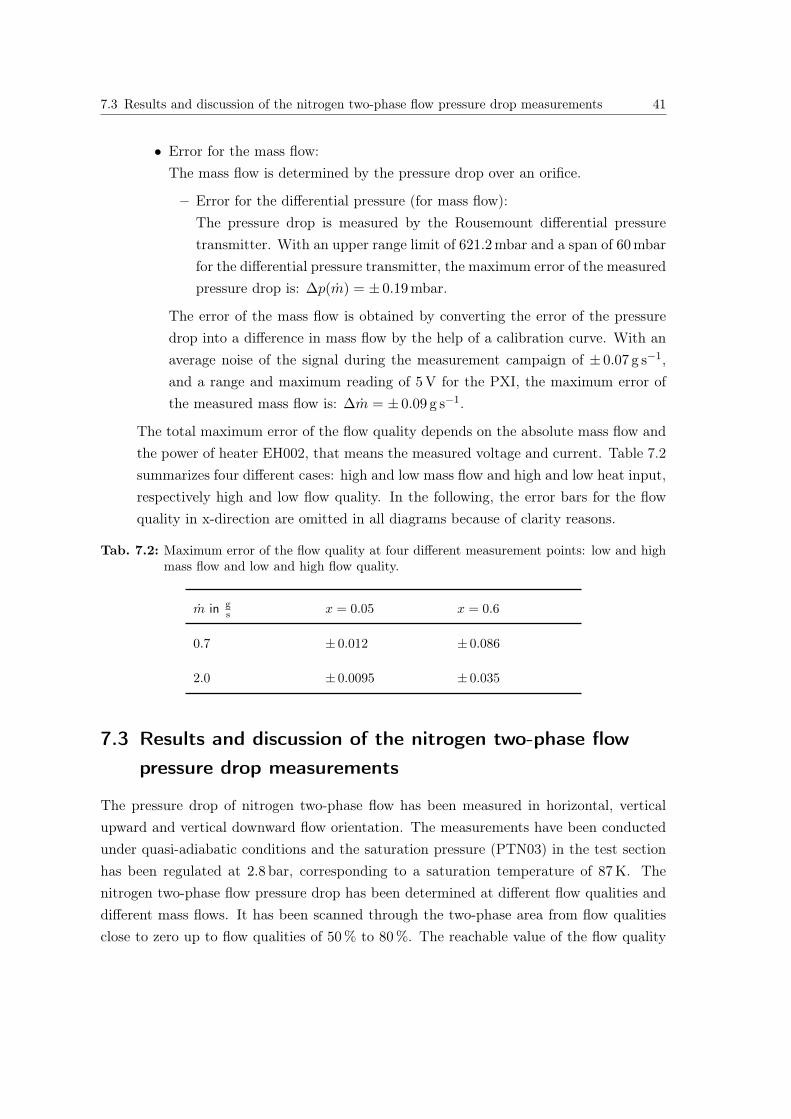
7.3 Results and discussion of the nitrogen two-phase flow pressure drop measurements 41
• Error for the mass flow:The mass flow is determined by the pressure drop over an orifice.
– Error for the differential pressure (for mass flow):The pressure drop is measured by the Rousemount differential pressuretransmitter. With an upper range limit of 621.2 mbar and a span of 60 mbar
for the differential pressure transmitter, the maximum error of the measuredpressure drop is: ∆p(m) = ± 0.19 mbar.
The error of the mass flow is obtained by converting the error of the pressuredrop into a difference in mass flow by the help of a calibration curve. With anaverage noise of the signal during the measurement campaign of ± 0.07 g s−1,and a range and maximum reading of 5 V for the PXI, the maximum error ofthe measured mass flow is: ∆m = ± 0.09 g s−1.
The total maximum error of the flow quality depends on the absolute mass flow andthe power of heater EH002, that means the measured voltage and current. Table 7.2summarizes four different cases: high and low mass flow and high and low heat input,respectively high and low flow quality. In the following, the error bars for the flowquality in x-direction are omitted in all diagrams because of clarity reasons.
Tab. 7.2: Maximum error of the flow quality at four different measurement points: low and highmass flow and low and high flow quality.
m in gs x = 0.05 x = 0.6
0.7 ± 0.012 ± 0.086
2.0 ± 0.0095 ± 0.035
7.3 Results and discussion of the nitrogen two-phase flowpressure drop measurements
The pressure drop of nitrogen two-phase flow has been measured in horizontal, verticalupward and vertical downward flow orientation. The measurements have been conductedunder quasi-adiabatic conditions and the saturation pressure (PTN03) in the test sectionhas been regulated at 2.8 bar, corresponding to a saturation temperature of 87 K. Thenitrogen two-phase flow pressure drop has been determined at different flow qualities anddifferent mass flows. It has been scanned through the two-phase area from flow qualitiesclose to zero up to flow qualities of 50 % to 80 %. The reachable value of the flow quality
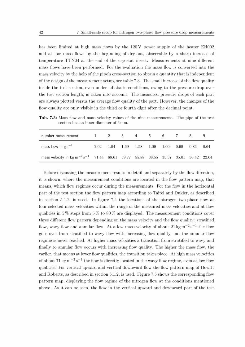
42 7 Small-scale setup for nitrogen two-phase flow pressure drop measurements
has been limited at high mass flows by the 120 V power supply of the heater EH002and at low mass flows by the beginning of dry-out, observable by a sharp increase oftemperature TTN04 at the end of the cryostat insert. Measurements at nine differentmass flows have been performed. For the evaluation the mass flow is converted into themass velocity by the help of the pipe’s cross-section to obtain a quantity that is independentof the design of the measurement setup, see table 7.3. The small increase of the flow qualityinside the test section, even under adiabatic conditions, owing to the pressure drop overthe test section length, is taken into account. The measured pressure drops of each partare always plotted versus the average flow quality of the part. However, the changes of theflow quality are only visible in the third or fourth digit after the decimal point.
Tab. 7.3: Mass flow and mass velocity values of the nine measurements. The pipe of the testsection has an inner diameter of 6 mm.
number measurement 1 2 3 4 5 6 7 8 9
mass flow in g s−1 2.02 1.94 1.69 1.58 1.09 1.00 0.99 0.86 0.64
mass velocity in kg m−2 s−1 71.44 68.61 59.77 55.88 38.55 35.37 35.01 30.42 22.64
Before discussing the measurement results in detail and separately by the flow direction,it is shown, where the measurement conditions are located in the flow pattern map, thatmeans, which flow regimes occur during the measurements. For the flow in the horizontalpart of the test section the flow pattern map according to Taitel and Dukler, as describedin section 5.1.2, is used. In figure 7.4 the locations of the nitrogen two-phase flow atfour selected mass velocities within the range of the measured mass velocities and at flowqualities in 5 % steps from 5 % to 80 % are displayed. The measurement conditions coverthree different flow pattern depending on the mass velocity and the flow quality: stratifiedflow, wavy flow and annular flow. At a low mass velocity of about 21 kg m−2 s−1 the flowgoes over from stratified to wavy flow with increasing flow quality, but the annular flowregime is never reached. At higher mass velocities a transition from stratified to wavy andfinally to annular flow occurs with increasing flow quality. The higher the mass flow, theearlier, that means at lower flow qualities, the transition takes place. At high mass velocitiesof about 71 kg m−2 s−1 the flow is directly located in the wavy flow regime, even at low flowqualities. For vertical upward and vertical downward flow the flow pattern map of Hewittand Roberts, as described in section 5.1.2, is used. Figure 7.5 shows the corresponding flowpattern map, displaying the flow regime of the nitrogen flow at the conditions mentionedabove. As it can be seen, the flow in the vertical upward and downward part of the test
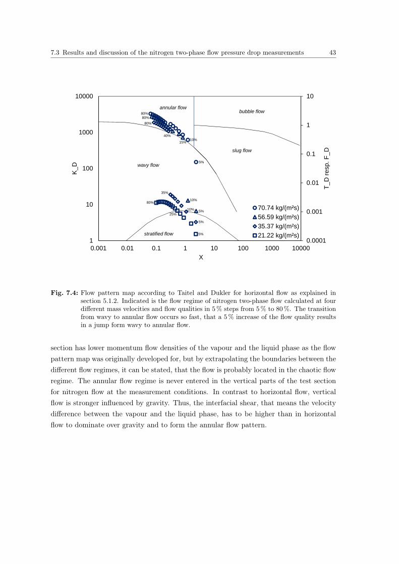
7.3 Results and discussion of the nitrogen two-phase flow pressure drop measurements 43
0.0001
0.001
0.01
0.1
1
10
1
10
100
1000
10000
0.001 0.01 0.1 1 10 100 1000 10000
T_D
resp
. F_D
K_D
X
70.74 kg/(m²s)56.59 kg/(m²s)35.37 kg/(m²s)21.22 kg/(m²s)
slug flow
annular flowbubble flow
wavy flow
stratified flow 5%
15%
25%
80%
5%
10%
35%
40%
80%80%
80%
5%10%
5%
10%
Fig. 7.4: Flow pattern map according to Taitel and Dukler for horizontal flow as explained insection 5.1.2. Indicated is the flow regime of nitrogen two-phase flow calculated at fourdifferent mass velocities and flow qualities in 5 % steps from 5 % to 80 %. The transitionfrom wavy to annular flow occurs so fast, that a 5 % increase of the flow quality resultsin a jump form wavy to annular flow.
section has lower momentum flow densities of the vapour and the liquid phase as the flowpattern map was originally developed for, but by extrapolating the boundaries between thedifferent flow regimes, it can be stated, that the flow is probably located in the chaotic flowregime. The annular flow regime is never entered in the vertical parts of the test sectionfor nitrogen flow at the measurement conditions. In contrast to horizontal flow, verticalflow is stronger influenced by gravity. Thus, the interfacial shear, that means the velocitydifference between the vapour and the liquid phase, has to be higher than in horizontalflow to dominate over gravity and to form the annular flow pattern.
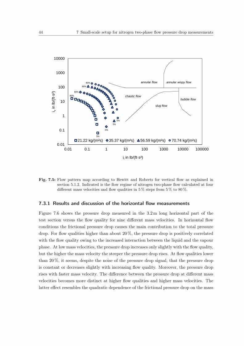
44 7 Small-scale setup for nitrogen two-phase flow pressure drop measurements
0.01
0.1
1
10
100
1000
10000
0.01 0.1 1 10 100 1000 10000 100000
i vin
lb/(f
t·s²)
il in lb/(ft·s²)
21.22 kg/(m²s) 35.37 kg/(m²s) 56.59 kg/(m²s) 70.74 kg/(m²s)
annular flow annular wispy flow
chaotic flow
slug flow
bubble flow
5%
5%
5%
5%
80%
80%
80%
80%
Fig. 7.5: Flow pattern map according to Hewitt and Roberts for vertical flow as explained insection 5.1.2. Indicated is the flow regime of nitrogen two-phase flow calculated at fourdifferent mass velocities and flow qualities in 5 % steps from 5 % to 80 %.
7.3.1 Results and discussion of the horizontal flow measurements
Figure 7.6 shows the pressure drop measured in the 3.2 m long horizontal part of thetest section versus the flow quality for nine different mass velocities. In horizontal flowconditions the frictional pressure drop causes the main contribution to the total pressuredrop. For flow qualities higher than about 20 %, the pressure drop is positively correlatedwith the flow quality owing to the increased interaction between the liquid and the vapourphase. At low mass velocities, the pressure drop increases only slightly with the flow quality,but the higher the mass velocity the steeper the pressure drop rises. At flow qualities lowerthan 20 %, it seems, despite the noise of the pressure drop signal, that the pressure dropis constant or decreases slightly with increasing flow quality. Moreover, the pressure droprises with faster mass velocity. The difference between the pressure drop at different massvelocities becomes more distinct at higher flow qualities and higher mass velocities. Thelatter effect resembles the quadratic dependence of the frictional pressure drop on the mass
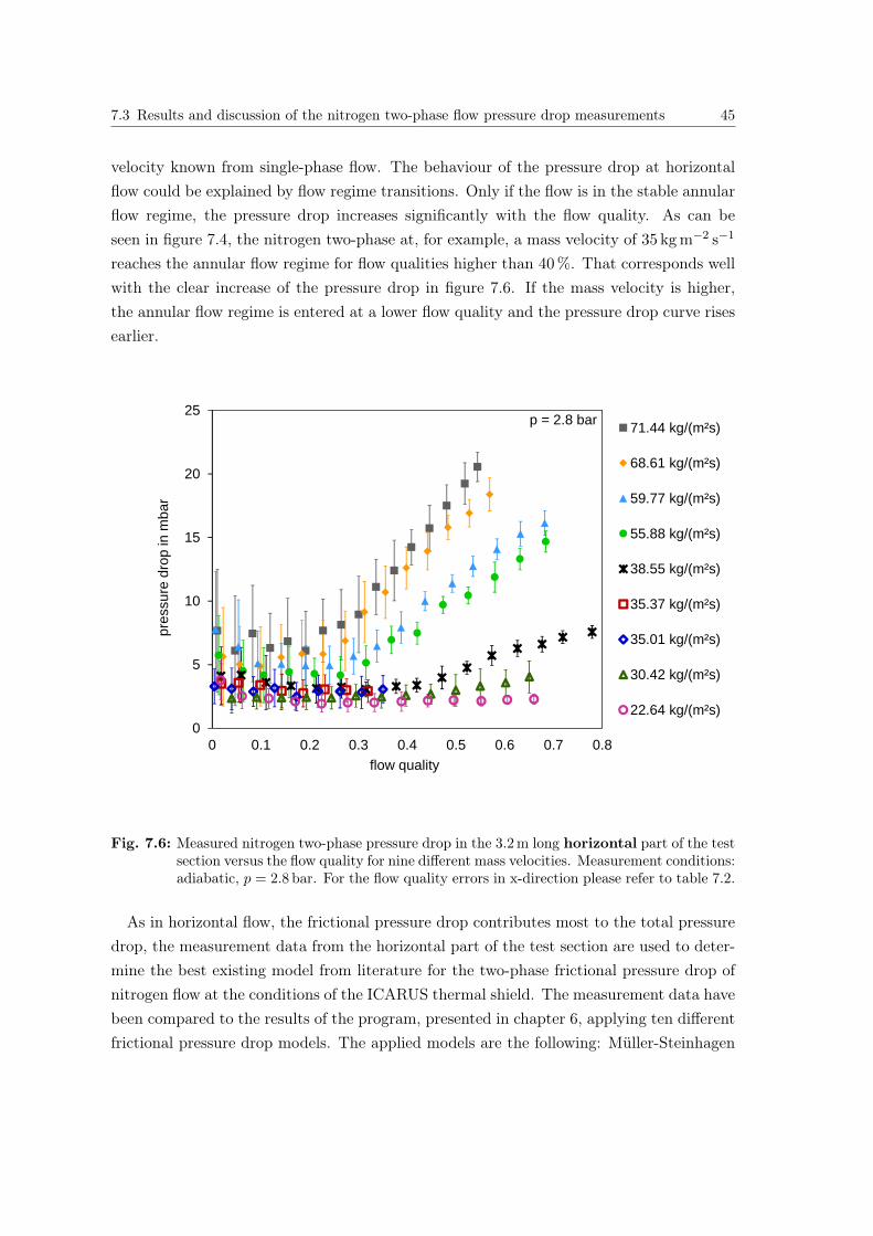
7.3 Results and discussion of the nitrogen two-phase flow pressure drop measurements 45
velocity known from single-phase flow. The behaviour of the pressure drop at horizontalflow could be explained by flow regime transitions. Only if the flow is in the stable annularflow regime, the pressure drop increases significantly with the flow quality. As can beseen in figure 7.4, the nitrogen two-phase at, for example, a mass velocity of 35 kg m−2 s−1
reaches the annular flow regime for flow qualities higher than 40 %. That corresponds wellwith the clear increase of the pressure drop in figure 7.6. If the mass velocity is higher,the annular flow regime is entered at a lower flow quality and the pressure drop curve risesearlier.
0
5
10
15
20
25
0 0.1 0.2 0.3 0.4 0.5 0.6 0.7 0.8
pres
sure
dro
p in
mba
r
flow quality
71.44 kg/(m²s)
68.61 kg/(m²s)
59.77 kg/(m²s)
55.88 kg/(m²s)
38.55 kg/(m²s)
35.37 kg/(m²s)
35.01 kg/(m²s)
30.42 kg/(m²s)
22.64 kg/(m²s)
p = 2.8 bar
Fig. 7.6: Measured nitrogen two-phase pressure drop in the 3.2 m long horizontal part of the testsection versus the flow quality for nine different mass velocities. Measurement conditions:adiabatic, p = 2.8 bar. For the flow quality errors in x-direction please refer to table 7.2.
As in horizontal flow, the frictional pressure drop contributes most to the total pressuredrop, the measurement data from the horizontal part of the test section are used to deter-mine the best existing model from literature for the two-phase frictional pressure drop ofnitrogen flow at the conditions of the ICARUS thermal shield. The measurement data havebeen compared to the results of the program, presented in chapter 6, applying ten differentfrictional pressure drop models. The applied models are the following: Müller-Steinhagen
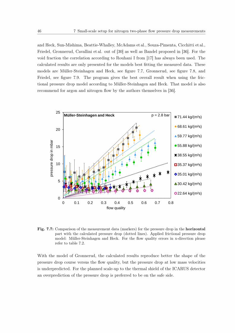
46 7 Small-scale setup for nitrogen two-phase flow pressure drop measurements
and Heck, Sun-Mishima, Beattie-Whalley, McAdams et al., Souza-Pimenta, Cicchitti et al.,Friedel, Gronnerud, Cavallini et al. out of [30] as well as Bandel proposed in [36]. For thevoid fraction the correlation according to Rouhani I from [17] has always been used. Thecalculated results are only presented for the models best fitting the measured data. Thesemodels are Müller-Steinhagen and Heck, see figure 7.7, Gronnerud, see figure 7.8, andFriedel, see figure 7.9. The program gives the best overall result when using the fric-tional pressure drop model according to Müller-Steinhagen and Heck. That model is alsorecommend for argon and nitrogen flow by the authors themselves in [36].
0
5
10
15
20
25
0 0.1 0.2 0.3 0.4 0.5 0.6 0.7 0.8
pres
sure
dro
p in
mba
r
flow quality
Müller-Steinhagen and Heck 71.44 kg/(m²s)
68.61 kg/(m²s)
59.77 kg/(m²s)
55.88 kg/(m²s)
38.55 kg/(m²s)
35.37 kg/(m²s)
35.01 kg/(m²s)
30.42 kg/(m²s)
22.64 kg/(m²s)
p = 2.8 bar
Fig. 7.7: Comparison of the measurement data (markers) for the pressure drop in the horizontalpart with the calculated pressure drop (dotted lines). Applied frictional pressure dropmodel: Müller-Steinhagen and Heck. For the flow quality errors in x-direction pleaserefer to table 7.2.
With the model of Gronnerud, the calculated results reproduce better the shape of thepressure drop course versus the flow quality, but the pressure drop at low mass velocitiesis underpredicted. For the planned scale-up to the thermal shield of the ICARUS detectoran overprediction of the pressure drop is preferred to be on the safe side.
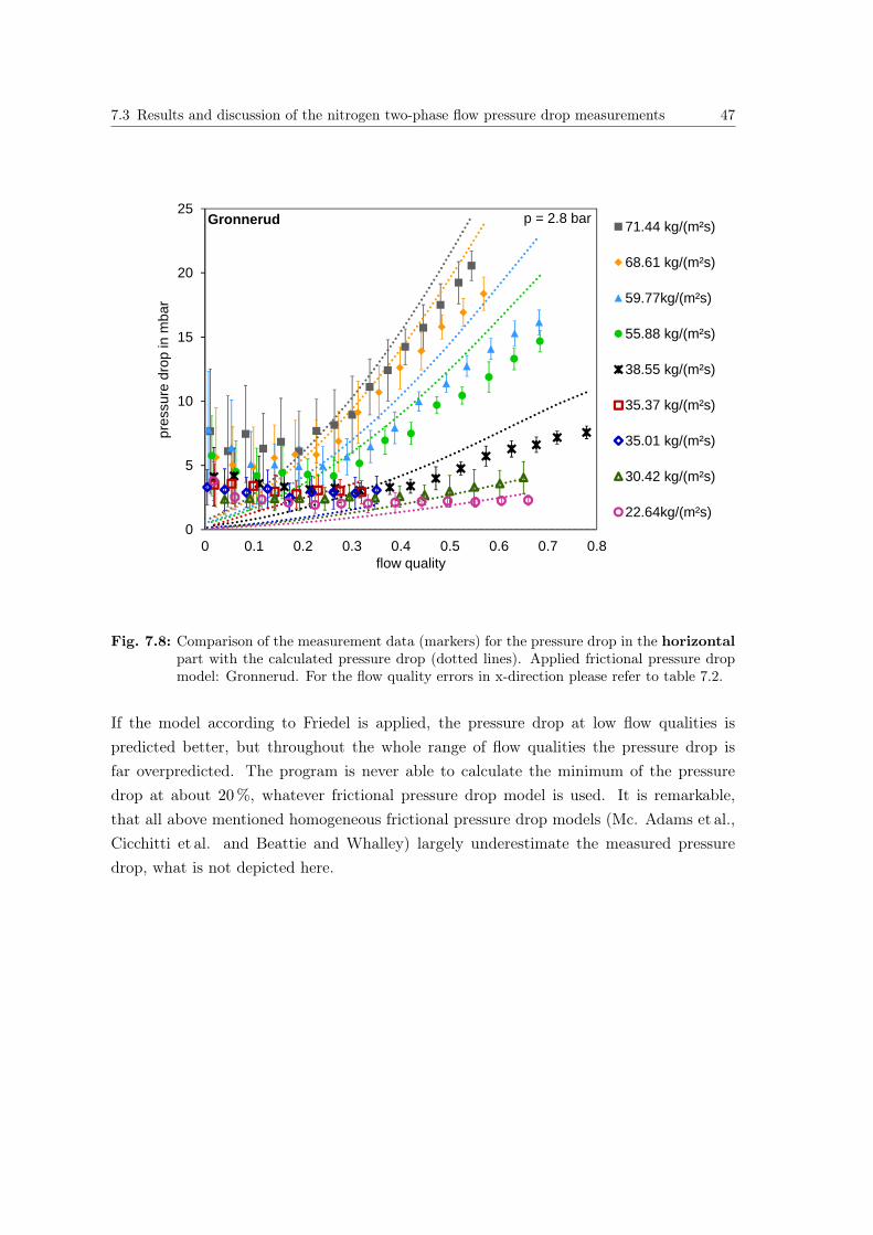
7.3 Results and discussion of the nitrogen two-phase flow pressure drop measurements 47
0
5
10
15
20
25
0 0.1 0.2 0.3 0.4 0.5 0.6 0.7 0.8
pres
sure
dro
p in
mba
r
flow quality
Gronnerud 71.44 kg/(m²s)
68.61 kg/(m²s)
59.77kg/(m²s)
55.88 kg/(m²s)
38.55 kg/(m²s)
35.37 kg/(m²s)
35.01 kg/(m²s)
30.42 kg/(m²s)
22.64kg/(m²s)
p = 2.8 bar
Fig. 7.8: Comparison of the measurement data (markers) for the pressure drop in the horizontalpart with the calculated pressure drop (dotted lines). Applied frictional pressure dropmodel: Gronnerud. For the flow quality errors in x-direction please refer to table 7.2.
If the model according to Friedel is applied, the pressure drop at low flow qualities ispredicted better, but throughout the whole range of flow qualities the pressure drop isfar overpredicted. The program is never able to calculate the minimum of the pressuredrop at about 20 %, whatever frictional pressure drop model is used. It is remarkable,that all above mentioned homogeneous frictional pressure drop models (Mc. Adams et al.,Cicchitti et al. and Beattie and Whalley) largely underestimate the measured pressuredrop, what is not depicted here.
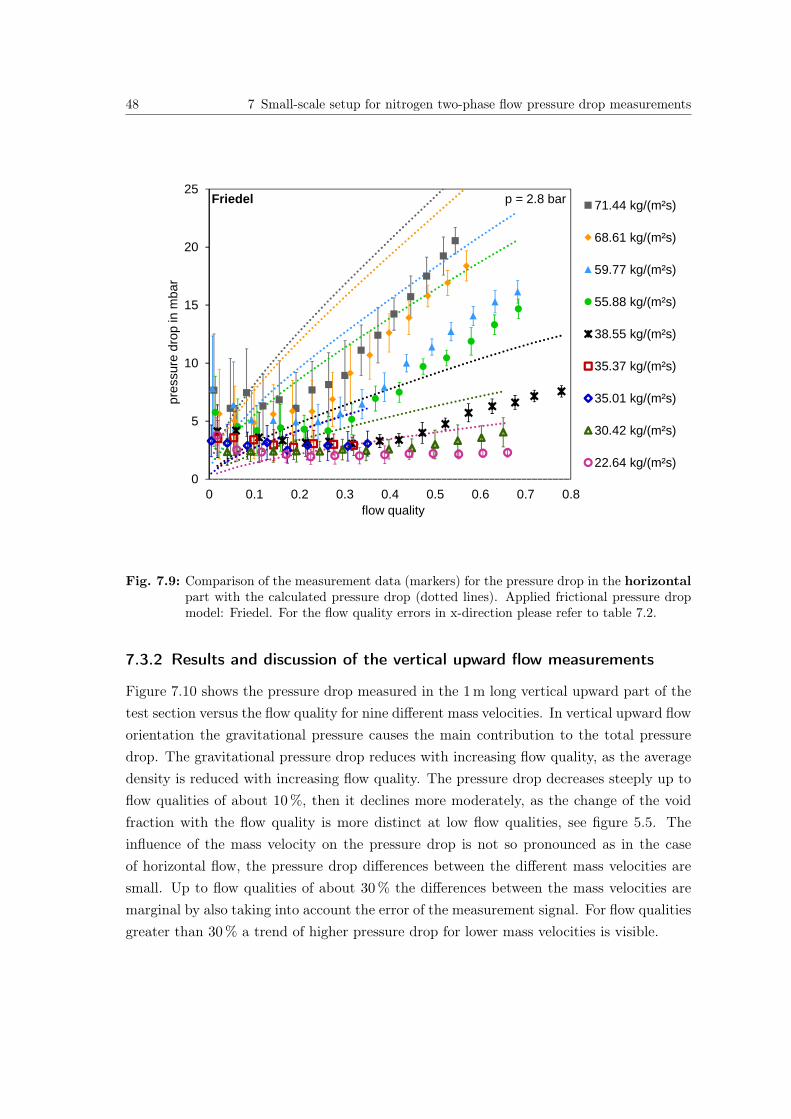
48 7 Small-scale setup for nitrogen two-phase flow pressure drop measurements
0
5
10
15
20
25
0 0.1 0.2 0.3 0.4 0.5 0.6 0.7 0.8
pres
sure
dro
p in
mba
r
flow quality
Friedel 71.44 kg/(m²s)
68.61 kg/(m²s)
59.77 kg/(m²s)
55.88 kg/(m²s)
38.55 kg/(m²s)
35.37 kg/(m²s)
35.01 kg/(m²s)
30.42 kg/(m²s)
22.64 kg/(m²s)
p = 2.8 bar
Fig. 7.9: Comparison of the measurement data (markers) for the pressure drop in the horizontalpart with the calculated pressure drop (dotted lines). Applied frictional pressure dropmodel: Friedel. For the flow quality errors in x-direction please refer to table 7.2.
7.3.2 Results and discussion of the vertical upward flow measurements
Figure 7.10 shows the pressure drop measured in the 1 m long vertical upward part of thetest section versus the flow quality for nine different mass velocities. In vertical upward floworientation the gravitational pressure causes the main contribution to the total pressuredrop. The gravitational pressure drop reduces with increasing flow quality, as the averagedensity is reduced with increasing flow quality. The pressure drop decreases steeply up toflow qualities of about 10 %, then it declines more moderately, as the change of the voidfraction with the flow quality is more distinct at low flow qualities, see figure 5.5. Theinfluence of the mass velocity on the pressure drop is not so pronounced as in the caseof horizontal flow, the pressure drop differences between the different mass velocities aresmall. Up to flow qualities of about 30 % the differences between the mass velocities aremarginal by also taking into account the error of the measurement signal. For flow qualitiesgreater than 30 % a trend of higher pressure drop for lower mass velocities is visible.
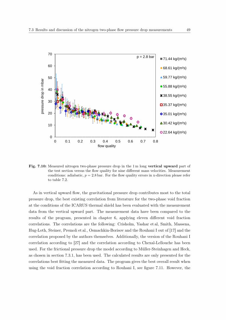
7.3 Results and discussion of the nitrogen two-phase flow pressure drop measurements 49
0
10
20
30
40
50
60
70
0 0.1 0.2 0.3 0.4 0.5 0.6 0.7 0.8
pres
sure
dro
p in
mba
r
flow quality
71.44 kg/(m²s)
68.61 kg/(m²s)
59.77 kg/(m²s)
55.88 kg/(m²s)
38.55 kg/(m²s)
35.37 kg/(m²s)
35.01 kg/(m²s)
30.42 kg/(m²s)
22.64 kg/(m²s)
p = 2.8 bar
Fig. 7.10: Measured nitrogen two-phase pressure drop in the 1 m long vertical upward part ofthe test section versus the flow quality for nine different mass velocities. Measurementconditions: adiabatic, p = 2.8 bar. For the flow quality errors in x-direction please referto table 7.2.
As in vertical upward flow, the gravitational pressure drop contributes most to the totalpressure drop, the best existing correlation from literature for the two-phase void fractionat the conditions of the ICARUS thermal shield has been evaluated with the measurementdata from the vertical upward part. The measurement data have been compared to theresults of the program, presented in chapter 6, applying eleven different void fractioncorrelations. The correlations are the following: Crisholm, Yashar et al, Smith, Massena,Hug-Loth, Steiner, Premoli et al., Osmachkin-Borisov and the Rouhani I out of [17] and thecorrelation proposed by the authors themselves. Additionally, the version of the Rouhani Icorrelation according to [27] and the correlation according to Chexal-Lellouche has beenused. For the frictional pressure drop the model according to Müller-Steinhagen and Heck,as chosen in section 7.3.1, has been used. The calculated results are only presented for thecorrelations best fitting the measured data. The program gives the best overall result whenusing the void fraction correlation according to Rouhani I, see figure 7.11. However, the
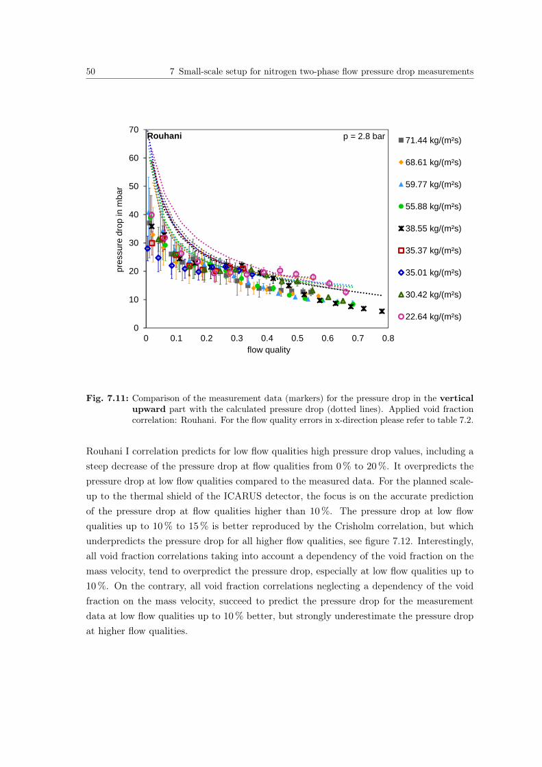
50 7 Small-scale setup for nitrogen two-phase flow pressure drop measurements
0
10
20
30
40
50
60
70
0 0.1 0.2 0.3 0.4 0.5 0.6 0.7 0.8
pres
sure
dro
p in
mba
r
flow quality
Rouhani 71.44 kg/(m²s)
68.61 kg/(m²s)
59.77 kg/(m²s)
55.88 kg/(m²s)
38.55 kg/(m²s)
35.37 kg/(m²s)
35.01 kg/(m²s)
30.42 kg/(m²s)
22.64 kg/(m²s)
p = 2.8 bar
Fig. 7.11: Comparison of the measurement data (markers) for the pressure drop in the verticalupward part with the calculated pressure drop (dotted lines). Applied void fractioncorrelation: Rouhani. For the flow quality errors in x-direction please refer to table 7.2.
Rouhani I correlation predicts for low flow qualities high pressure drop values, including asteep decrease of the pressure drop at flow qualities from 0 % to 20 %. It overpredicts thepressure drop at low flow qualities compared to the measured data. For the planned scale-up to the thermal shield of the ICARUS detector, the focus is on the accurate predictionof the pressure drop at flow qualities higher than 10 %. The pressure drop at low flowqualities up to 10 % to 15 % is better reproduced by the Crisholm correlation, but whichunderpredicts the pressure drop for all higher flow qualities, see figure 7.12. Interestingly,all void fraction correlations taking into account a dependency of the void fraction on themass velocity, tend to overpredict the pressure drop, especially at low flow qualities up to10 %. On the contrary, all void fraction correlations neglecting a dependency of the voidfraction on the mass velocity, succeed to predict the pressure drop for the measurementdata at low flow qualities up to 10 % better, but strongly underestimate the pressure dropat higher flow qualities.
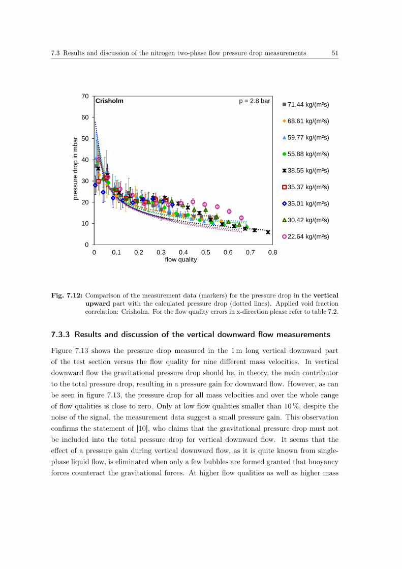
7.3 Results and discussion of the nitrogen two-phase flow pressure drop measurements 51
0
10
20
30
40
50
60
70
0 0.1 0.2 0.3 0.4 0.5 0.6 0.7 0.8
pres
sure
dro
p in
mba
r
flow quality
Crisholm 71.44 kg/(m²s)
68.61 kg/(m²s)
59.77 kg/(m²s)
55.88 kg/(m²s)
38.55 kg/(m²s)
35.37 kg/(m²s)
35.01 kg/(m²s)
30.42 kg/(m²s)
22.64 kg/(m²s)
p = 2.8 bar
Fig. 7.12: Comparison of the measurement data (markers) for the pressure drop in the verticalupward part with the calculated pressure drop (dotted lines). Applied void fractioncorrelation: Crisholm. For the flow quality errors in x-direction please refer to table 7.2.
7.3.3 Results and discussion of the vertical downward flow measurements
Figure 7.13 shows the pressure drop measured in the 1 m long vertical downward partof the test section versus the flow quality for nine different mass velocities. In verticaldownward flow the gravitational pressure drop should be, in theory, the main contributorto the total pressure drop, resulting in a pressure gain for downward flow. However, as canbe seen in figure 7.13, the pressure drop for all mass velocities and over the whole rangeof flow qualities is close to zero. Only at low flow qualities smaller than 10 %, despite thenoise of the signal, the measurement data suggest a small pressure gain. This observationconfirms the statement of [10], who claims that the gravitational pressure drop must notbe included into the total pressure drop for vertical downward flow. It seems that theeffect of a pressure gain during vertical downward flow, as it is quite known from single-phase liquid flow, is eliminated when only a few bubbles are formed granted that buoyancyforces counteract the gravitational forces. At higher flow qualities as well as higher mass
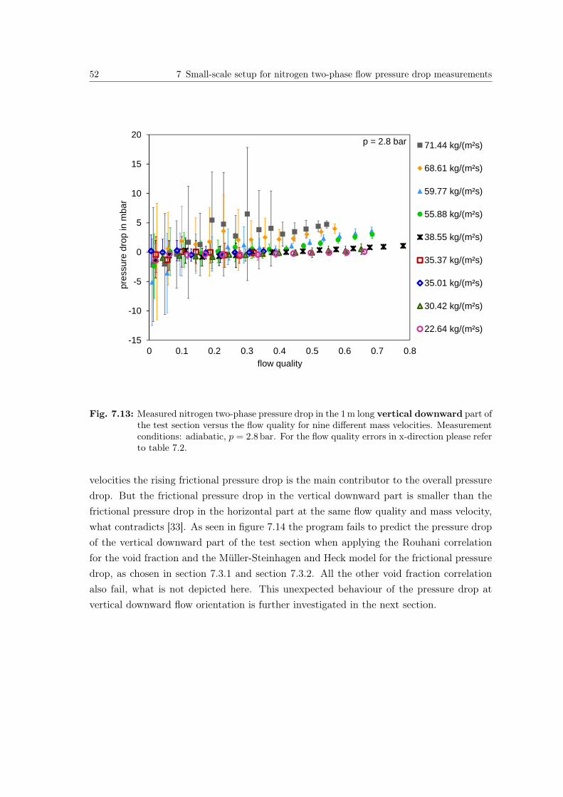
52 7 Small-scale setup for nitrogen two-phase flow pressure drop measurements
-15
-10
-5
0
5
10
15
20
0 0.1 0.2 0.3 0.4 0.5 0.6 0.7 0.8
pres
sure
dro
p in
mba
r
flow quality
71.44 kg/(m²s)
68.61 kg/(m²s)
59.77 kg/(m²s)
55.88 kg/(m²s)
38.55 kg/(m²s)
35.37 kg/(m²s)
35.01 kg/(m²s)
30.42 kg/(m²s)
22.64 kg/(m²s)
p = 2.8 bar
Fig. 7.13: Measured nitrogen two-phase pressure drop in the 1 m long vertical downward part ofthe test section versus the flow quality for nine different mass velocities. Measurementconditions: adiabatic, p = 2.8 bar. For the flow quality errors in x-direction please referto table 7.2.
velocities the rising frictional pressure drop is the main contributor to the overall pressuredrop. But the frictional pressure drop in the vertical downward part is smaller than thefrictional pressure drop in the horizontal part at the same flow quality and mass velocity,what contradicts [33]. As seen in figure 7.14 the program fails to predict the pressure dropof the vertical downward part of the test section when applying the Rouhani correlationfor the void fraction and the Müller-Steinhagen and Heck model for the frictional pressuredrop, as chosen in section 7.3.1 and section 7.3.2. All the other void fraction correlationalso fail, what is not depicted here. This unexpected behaviour of the pressure drop atvertical downward flow orientation is further investigated in the next section.
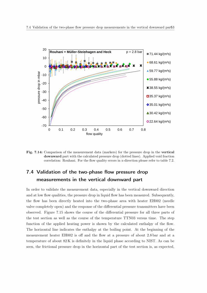
7.4 Validation of the two-phase flow pressure drop measurements in the vertical downward part53
-70
-60
-50
-40
-30
-20
-10
0
10
20
0 0.1 0.2 0.3 0.4 0.5 0.6 0.7 0.8
pres
sure
dro
p in
mba
r
flow quality
Rouhani + Müller-Steinhagen and Heck 71.44 kg/(m²s)
68.61 kg/(m²s)
59.77 kg/(m²s)
55.88 kg/(m²s)
38.55 kg/(m²s)
35.37 kg/(m²s)
35.01 kg/(m²s)
30.42 kg/(m²s)
22.64 kg/(m²s)
p = 2.8 bar
Fig. 7.14: Comparison of the measurement data (markers) for the pressure drop in the verticaldownward part with the calculated pressure drop (dotted lines). Applied void fractioncorrelation: Rouhani. For the flow quality errors in x-direction please refer to table 7.2.
7.4 Validation of the two-phase flow pressure dropmeasurements in the vertical downward part
In order to validate the measurement data, especially in the vertical downward directionand at low flow qualities, the pressure drop in liquid flow has been measured. Subsequently,the flow has been directly heated into the two-phase area with heater EH002 (needlevalve completely open) and the response of the differential pressure transmitters have beenobserved. Figure 7.15 shows the course of the differential pressure for all three parts ofthe test section as well as the course of the temperature TTN03 versus time. The stepfunction of the applied heating power is shown by the calculated enthalpy of the flow.The horizontal line indicates the enthalpy at the boiling point. At the beginning of themeasurement heater EH002 is off and the flow at a pressure of about 2.8 bar and at atemperature of about 82 K is definitely in the liquid phase according to NIST. As can beseen, the frictional pressure drop in the horizontal part of the test section is, as expected,
54 7 Small-scale setup for nitrogen two-phase flow pressure drop measurements
extremely small. Because the lower limit of the differential pressure sensor for the horizontalpart is 0 mbar, the noise of the sensor seems to be only in the direction of positive values.The pressure loss in the vertical upward part and the pressure gain in the vertical downwardpart are the same, according to the absolute value, and also correspond to the expectedvalue in liquid flow. Then, the heater EH002 is switched on and increased stepwise untila flow quality of about 8 % is reached. Temperature TTN03 indicates from which time onthe flow has reached the two-phase area. According to NIST, the saturation temperaturecorresponding to the saturation pressure of 2.8 bar is about 87 K. One can observe that,even shortly before the flow reaches two-phase conditions, probably when the first bubblesare formed locally in the heater, the pressure gain in the vertical downward part jumps toa value close to zero. The pressure loss in the vertical upward part only drops when thetwo-phase conditions are reached and it drops in a more moderate way. When the heaterpower is reduced again, mirror-inverted to switching on the heater, firstly the pressuredrop in the vertical upward part sharply increases again, whereas the pressure gain onthe vertical downward part rises with some time delay. In summary, two observations canbe made. Firstly, the pressure gain in vertical downward flow can be measured correctlywith the experimental setup for liquid flow, proofing that the pressure gain in verticaldownward two-phase flow is negligible. Secondly, entering the two-phase area by heatingcauses delay in boiling and the flow is not in thermodynamic equilibrium as, for verticalupward flow, the same pressure drop values as in liquid flow are measured at a time whenthe flow is theoretically already in two-phase conditions. The measurement data for thepressure drop in vertical upward flow at low flow qualities is lower than the predicted one,because in the measurements described before in section 7.3 the two-phase area is enteredby a Joule-Thomson expansion forcing the flow instantly into thermodynamic equilibrium.This is one possible explanation for the differences for low flow quality described by themodels and former studies and the here presented measurement data.
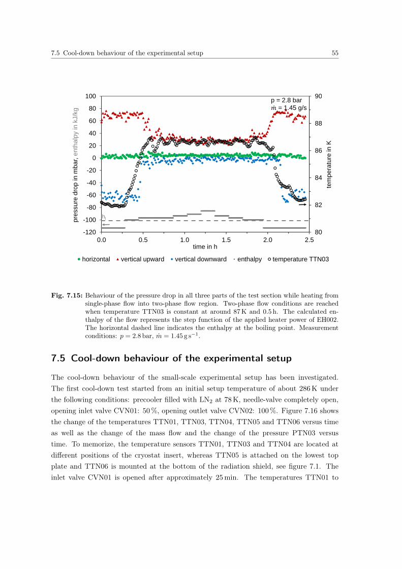
7.5 Cool-down behaviour of the experimental setup 55
80
82
84
86
88
90
-120
-100
-80
-60
-40
-20
0
20
40
60
80
100
0.0 0.5 1.0 1.5 2.0 2.5
tem
pera
ture
in K
pres
sure
dro
p in
mba
r, en
thal
py in
kJ/
kg
time in h
horizontal vertical upward vertical downward enthalpy temperature TTN03
p = 2.8 bar푚 = 1.45 g/s
hl
Fig. 7.15: Behaviour of the pressure drop in all three parts of the test section while heating fromsingle-phase flow into two-phase flow region. Two-phase flow conditions are reachedwhen temperature TTN03 is constant at around 87 K and 0.5 h. The calculated en-thalpy of the flow represents the step function of the applied heater power of EH002.The horizontal dashed line indicates the enthalpy at the boiling point. Measurementconditions: p = 2.8 bar, m = 1.45 g s−1.
7.5 Cool-down behaviour of the experimental setup
The cool-down behaviour of the small-scale experimental setup has been investigated.The first cool-down test started from an initial setup temperature of about 286 K underthe following conditions: precooler filled with LN2 at 78 K, needle-valve completely open,opening inlet valve CVN01: 50%, opening outlet valve CVN02: 100%. Figure 7.16 showsthe change of the temperatures TTN01, TTN03, TTN04, TTN05 and TTN06 versus timeas well as the change of the mass flow and the change of the pressure PTN03 versustime. To memorize, the temperature sensors TTN01, TTN03 and TTN04 are located atdifferent positions of the cryostat insert, whereas TTN05 is attached on the lowest topplate and TTN06 is mounted at the bottom of the radiation shield, see figure 7.1. Theinlet valve CVN01 is opened after approximately 25 min. The temperatures TTN01 to
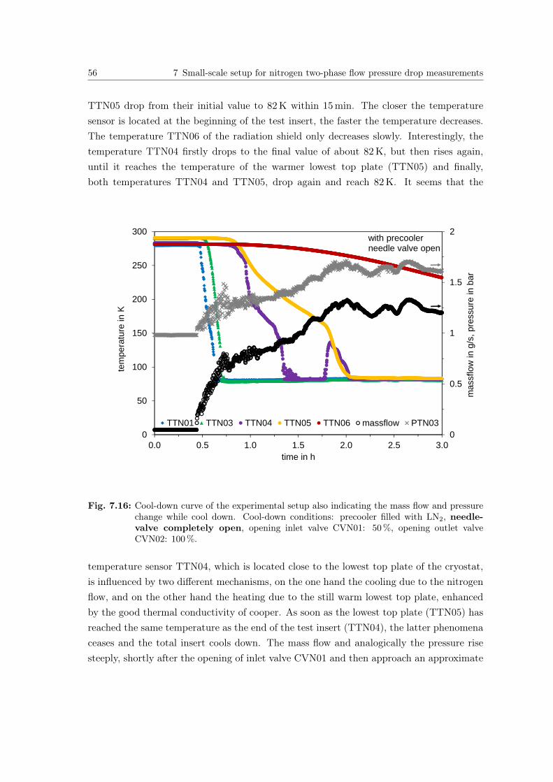
56 7 Small-scale setup for nitrogen two-phase flow pressure drop measurements
TTN05 drop from their initial value to 82 K within 15 min. The closer the temperaturesensor is located at the beginning of the test insert, the faster the temperature decreases.The temperature TTN06 of the radiation shield only decreases slowly. Interestingly, thetemperature TTN04 firstly drops to the final value of about 82 K, but then rises again,until it reaches the temperature of the warmer lowest top plate (TTN05) and finally,both temperatures TTN04 and TTN05, drop again and reach 82 K. It seems that the
0
0.5
1
1.5
2
0
50
100
150
200
250
300
0.0 0.5 1.0 1.5 2.0 2.5 3.0
mas
sflo
w in
g/s
, pre
ssur
e in
bar
tem
pera
ture
in K
time in h
TTN01 TTN03 TTN04 TTN05 TTN06 massflow PTN03
with precoolerneedle valve open
Fig. 7.16: Cool-down curve of the experimental setup also indicating the mass flow and pressurechange while cool down. Cool-down conditions: precooler filled with LN2, needle-valve completely open, opening inlet valve CVN01: 50%, opening outlet valveCVN02: 100%.
temperature sensor TTN04, which is located close to the lowest top plate of the cryostat,is influenced by two different mechanisms, on the one hand the cooling due to the nitrogenflow, and on the other hand the heating due to the still warm lowest top plate, enhancedby the good thermal conductivity of cooper. As soon as the lowest top plate (TTN05) hasreached the same temperature as the end of the test insert (TTN04), the latter phenomenaceases and the total insert cools down. The mass flow and analogically the pressure risesteeply, shortly after the opening of inlet valve CVN01 and then approach an approximate
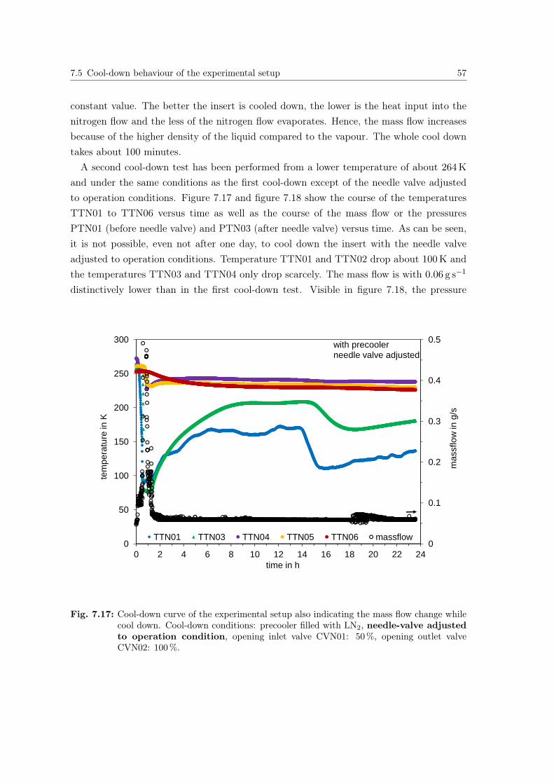
7.5 Cool-down behaviour of the experimental setup 57
constant value. The better the insert is cooled down, the lower is the heat input into thenitrogen flow and the less of the nitrogen flow evaporates. Hence, the mass flow increasesbecause of the higher density of the liquid compared to the vapour. The whole cool downtakes about 100 minutes.A second cool-down test has been performed from a lower temperature of about 264 K
and under the same conditions as the first cool-down except of the needle valve adjustedto operation conditions. Figure 7.17 and figure 7.18 show the course of the temperaturesTTN01 to TTN06 versus time as well as the course of the mass flow or the pressuresPTN01 (before needle valve) and PTN03 (after needle valve) versus time. As can be seen,it is not possible, even not after one day, to cool down the insert with the needle valveadjusted to operation conditions. Temperature TTN01 and TTN02 drop about 100 K andthe temperatures TTN03 and TTN04 only drop scarcely. The mass flow is with 0.06 g s−1
distinctively lower than in the first cool-down test. Visible in figure 7.18, the pressure
0
0.1
0.2
0.3
0.4
0.5
0
50
100
150
200
250
300
0 2 4 6 8 10 12 14 16 18 20 22 24
mas
sflo
w in
g/s
tem
pera
ture
in K
time in h
TTN01 TTN03 TTN04 TTN05 TTN06 massflow
with precoolerneedle valve adjusted
Fig. 7.17: Cool-down curve of the experimental setup also indicating the mass flow change whilecool down. Cool-down conditions: precooler filled with LN2, needle-valve adjustedto operation condition, opening inlet valve CVN01: 50%, opening outlet valveCVN02: 100%.
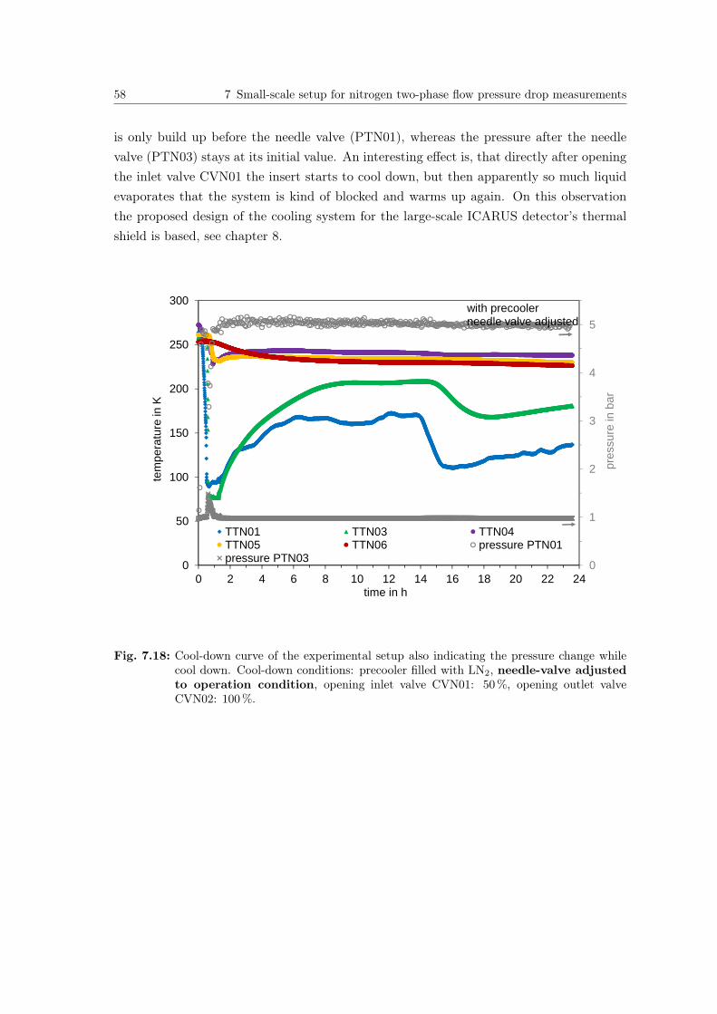
58 7 Small-scale setup for nitrogen two-phase flow pressure drop measurements
is only build up before the needle valve (PTN01), whereas the pressure after the needlevalve (PTN03) stays at its initial value. An interesting effect is, that directly after openingthe inlet valve CVN01 the insert starts to cool down, but then apparently so much liquidevaporates that the system is kind of blocked and warms up again. On this observationthe proposed design of the cooling system for the large-scale ICARUS detector’s thermalshield is based, see chapter 8.
0
1
2
3
4
5
0
50
100
150
200
250
300
0 2 4 6 8 10 12 14 16 18 20 22 24
pres
sure
in b
ar
tem
pera
ture
in K
time in h
TTN01 TTN03 TTN04TTN05 TTN06 pressure PTN01pressure PTN03
with precoolerneedle valve adjusted
Fig. 7.18: Cool-down curve of the experimental setup also indicating the pressure change whilecool down. Cool-down conditions: precooler filled with LN2, needle-valve adjustedto operation condition, opening inlet valve CVN01: 50%, opening outlet valveCVN02: 100%.
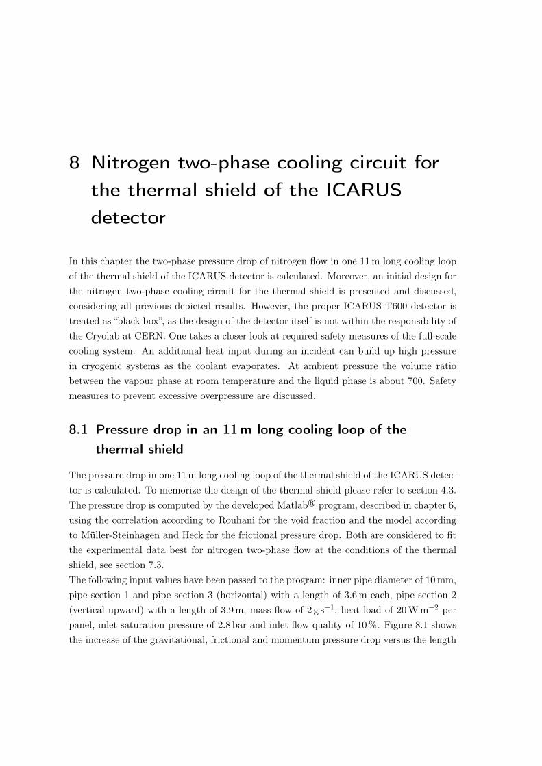
8 Nitrogen two-phase cooling circuit forthe thermal shield of the ICARUSdetector
In this chapter the two-phase pressure drop of nitrogen flow in one 11m long cooling loopof the thermal shield of the ICARUS detector is calculated. Moreover, an initial design forthe nitrogen two-phase cooling circuit for the thermal shield is presented and discussed,considering all previous depicted results. However, the proper ICARUS T600 detector istreated as “black box”, as the design of the detector itself is not within the responsibility ofthe Cryolab at CERN. One takes a closer look at required safety measures of the full-scalecooling system. An additional heat input during an incident can build up high pressurein cryogenic systems as the coolant evaporates. At ambient pressure the volume ratiobetween the vapour phase at room temperature and the liquid phase is about 700. Safetymeasures to prevent excessive overpressure are discussed.
8.1 Pressure drop in an 11m long cooling loop of thethermal shield
The pressure drop in one 11m long cooling loop of the thermal shield of the ICARUS detec-tor is calculated. To memorize the design of the thermal shield please refer to section 4.3.The pressure drop is computed by the developed Matlab R© program, described in chapter 6,using the correlation according to Rouhani for the void fraction and the model accordingto Müller-Steinhagen and Heck for the frictional pressure drop. Both are considered to fitthe experimental data best for nitrogen two-phase flow at the conditions of the thermalshield, see section 7.3.The following input values have been passed to the program: inner pipe diameter of 10 mm,pipe section 1 and pipe section 3 (horizontal) with a length of 3.6 m each, pipe section 2(vertical upward) with a length of 3.9 m, mass flow of 2 g s−1, heat load of 20 W m−2 perpanel, inlet saturation pressure of 2.8 bar and inlet flow quality of 10 %. Figure 8.1 showsthe increase of the gravitational, frictional and momentum pressure drop versus the length
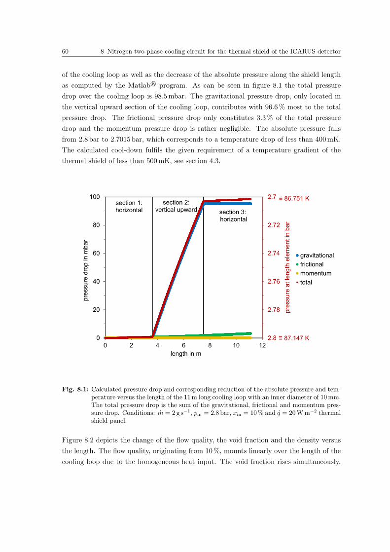
60 8 Nitrogen two-phase cooling circuit for the thermal shield of the ICARUS detector
of the cooling loop as well as the decrease of the absolute pressure along the shield lengthas computed by the Matlab R© program. As can be seen in figure 8.1 the total pressuredrop over the cooling loop is 98.5 mbar. The gravitational pressure drop, only located inthe vertical upward section of the cooling loop, contributes with 96.6 % most to the totalpressure drop. The frictional pressure drop only constitutes 3.3 % of the total pressuredrop and the momentum pressure drop is rather negligible. The absolute pressure fallsfrom 2.8 bar to 2.7015 bar, which corresponds to a temperature drop of less than 400 mK.The calculated cool-down fulfils the given requirement of a temperature gradient of thethermal shield of less than 500 mK, see section 4.3.
2.7
2.72
2.74
2.76
2.78
2.80
20
40
60
80
100
0 2 4 6 8 10 12
pre
ssure
at
length
ele
ment
in b
ar
pre
ssure
dro
p in m
bar
length in m
gravitational
frictional
momentum
total
≡ 86.751 K
≡ 87.147 K
section 1:horizontal
section 2: vertical upward section 3:
horizontal
Fig. 8.1: Calculated pressure drop and corresponding reduction of the absolute pressure and tem-perature versus the length of the 11m long cooling loop with an inner diameter of 10 mm.The total pressure drop is the sum of the gravitational, frictional and momentum pres-sure drop. Conditions: m = 2 g s−1, pin = 2.8 bar, xin = 10 % and q = 20 W m−2 thermalshield panel.
Figure 8.2 depicts the change of the flow quality, the void fraction and the density versusthe length. The flow quality, originating from 10 %, mounts linearly over the length of thecooling loop due to the homogeneous heat input. The void fraction rises simultaneously,
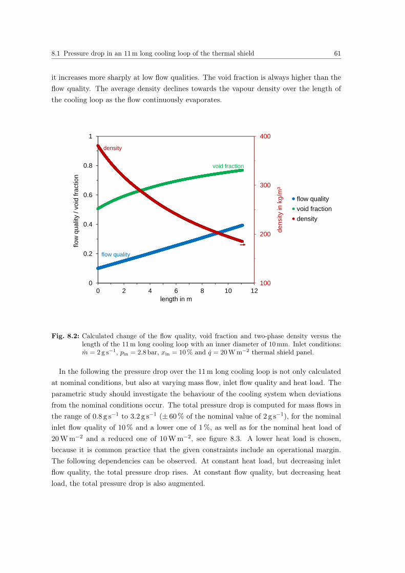
8.1 Pressure drop in an 11m long cooling loop of the thermal shield 61
it increases more sharply at low flow qualities. The void fraction is always higher than theflow quality. The average density declines towards the vapour density over the length ofthe cooling loop as the flow continuously evaporates.
100
200
300
400
0
0.2
0.4
0.6
0.8
1
0 2 4 6 8 10 12
dens
ity in
kg/
m³
flow
qua
lity
/ voi
d fra
ctio
n
length in m
flow qualityvoid fractiondensity
void fraction
density
flow quality
Fig. 8.2: Calculated change of the flow quality, void fraction and two-phase density versus thelength of the 11m long cooling loop with an inner diameter of 10 mm. Inlet conditions:m = 2 g s−1, pin = 2.8 bar, xin = 10 % and q = 20 W m−2 thermal shield panel.
In the following the pressure drop over the 11m long cooling loop is not only calculatedat nominal conditions, but also at varying mass flow, inlet flow quality and heat load. Theparametric study should investigate the behaviour of the cooling system when deviationsfrom the nominal conditions occur. The total pressure drop is computed for mass flows inthe range of 0.8 g s−1 to 3.2 g s−1 (± 60 % of the nominal value of 2 g s−1), for the nominalinlet flow quality of 10 % and a lower one of 1 %, as well as for the nominal heat load of20 W m−2 and a reduced one of 10 W m−2, see figure 8.3. A lower heat load is chosen,because it is common practice that the given constraints include an operational margin.The following dependencies can be observed. At constant heat load, but decreasing inletflow quality, the total pressure drop rises. At constant flow quality, but decreasing heatload, the total pressure drop is also augmented.
62 8 Nitrogen two-phase cooling circuit for the thermal shield of the ICARUS detector
0
40
80
120
160
0.8 1.3 1.8 2.3 2.8
pres
sure
dro
p in
mba
r
massflow in g/s
x_in = 10 %, q_dot = 20 W/m² x_in = 10 %, q_dot = 10 W/m²x_in = 1 %, q_dot = 20 W/m² x_in = 1 %, q_dot= 10 W/m²
d = 10 mm
Fig. 8.3: Total pressure drop over the 11m long cooling loop with an inner diameter of 10mmversus mass flow in the range of 0.8 g s−1 to 3.2 g s−1. Parametric study for differentcombination of xin = 1 %, xin = 10 % and q = 10 W m−2, q = 20 W m−2 at pin = 2.8 bar.
To memorize, the gravitational pressure drop is the biggest contributor to the total pressuredrop. In both cases, the average flow quality along the loop is reduced, and consequently,the average two-phase density increases, resulting in a higher gravitational pressure drop.The dependency of the total pressure drop on the mass flow is more complex. At low inletflow qualities of 1 % the total pressure drop and the mass flow are positively correlated. Athigh inlet flow qualities of 10 % and a heat load of 20 W m−2 the total pressure drop is nearlyconstant over the mass flow range, whereas at a heat load of 10 W m−2 the total pressureis negatively correlated with the mass flow. To memorize, the void fraction according tothe correlation of Rouhani increases with rising flow quality as well as rising mass velocity.At constant inlet flow quality and constant heat load, but higher mass flow, the outlet flowquality diminishes. Depending on the absolute value of both, the flow quality and the massvelocity, either the effect of increased mass velocity or the effect of reduced flow qualitydominates. In the former case the void fraction rises, leading to a lower gravitationalpressure drop. In the latter case of reduced flow quality the void fraction drops, resulting
8.1 Pressure drop in an 11m long cooling loop of the thermal shield 63
in a higher gravitational pressure drop. The flow quality effect seems to outweigh the massvelocity effect rather at low flow qualities because the slope of the void fraction versus theflow quality is larger at low flow qualities, see figure 5.5. In the case, in which the effect ofincreasing mass flow predominates the effect of reduced flow quality, and the pressure dropand the mass flow are negatively correlated, the cooling system destabilizes itself and canrun into a dry-out. Assuming that the mass flow temporarily decreases in one of the 42
parallel cooling loops due to mass flow fluctuations, the pressure drop in this cooling loopis higher compared to the other cooling loops, preventing fluid to sufficiently enter thiscooling loop and causing a dry-out. With smaller pipe diameter, that means, higher massvelocity, the dependency of the void fraction according to Rouhani on the mass velocity isdiminished, see figure 5.6, and consequently, the effect of the flow quality starts to alwayspredominate the effect of the mass velocity, see figure 8.4.
0
40
80
120
160
0.8 1.3 1.8 2.3 2.8
pres
sure
dro
p in
mba
r
massflow in g/s
x_in = 10 %, q_dot = 20 W/m² x_in = 10 %, q_dot = 10 W/m²x_in = 1 %, q_dot = 20 W/m² x_in = 1 %, q_dot = 10 W/m²
d = 8 mm
Fig. 8.4: Total pressure drop over the 11m long cooling loop with an inner diameter of 8mmversus mass flow in the range of 0.8 g s−1 to 3.2 g s−1. Parametric study for differentcombination of xin = 1 %, xin = 10 % and q = 10 W m−2, q = 20 W m−2 at pin = 2.8 bar.
At a pipe diameter of 6 mm the destabilizing effect is even eliminated as the pressuredrop and the mass flow are always positively correlated, see figure 8.5. The differences
64 8 Nitrogen two-phase cooling circuit for the thermal shield of the ICARUS detector
between various inlet flow qualities or various heat loads become less distinct at low pipediameters. For a pipe diameter of 6 mm and nominal conditions with an inlet flow qualityof 10 % and a heat load of 20 W m−2 s−1 the total pressure drop along the cooling loopincreases to 108 mbar. Nonetheless, with a corresponding temperature drop of 433 mK therequirements regarding the temperature gradient along the thermal shield are fulfilled.
0
40
80
120
160
0.8 1.3 1.8 2.3 2.8
pres
sure
dro
p in
mba
r
massflow in g/s
x_in = 10 %, q_dot = 20 W/m² x_in = 10 %, q_dot = 10 W/m²x_in = 1 %, q_dot = 20 W/m² x_in = 1 %, q_dot = 10 W/m²
d = 6 mm
Fig. 8.5: Total pressure drop over the 11m long cooling loop with an inner diameter of 6mmversus mass flow in the range of 0.8 g s−1 to 3.2 g s−1. Parametric study for differentcombination of xin = 1 %, xin = 10 % and q = 10 W m−2, q = 20 W m−2 at pin = 2.8 bar.
In figure 8.6 and figure 8.8 (flow pattern map for horizontal flow according to Taitel andDukler) as well as figure 8.7 and figure 8.9 (flow pattern map for vertical flow according toHewitt and Roberts) it can be seen which flow pattern will occur in the 11m long coolingloop with an inner diameter of 10 mm or 6 mm. The lowest discussed mass flow of 0.8 g s−1,the nominal mass flow of 2.0 g s−1 and the highest discussed mass flow of 3.2 g s−1 as wellas all combinations of the inlet flow qualities and heat loads are included in the maps. Themarkers represent always the inlet and the outlet condition of each section of the coolingpanels. As the cooling loop has two horizontal, but only one vertical upward section,there are four markers in the horizontal flow pattern map for each condition, but only two
8.1 Pressure drop in an 11m long cooling loop of the thermal shield 65
markers in the vertical flow pattern map. For an inner pipe diameter of 10 mm stratified orwavy flow occur in the horizontal sections and chaotic flow occurs in the vertical upwardsection.
0.0001
0.001
0.01
0.1
1
10
1
10
100
1000
10000
0.001 0.01 0.1 1 10 100 1000 10000
T_D
resp
. F_D
K_D
X
slug flow
annular flowbubble flow
wavy flow
stratified flow
circle: 0.8 g/ssquare: 2.0 g/striangle: 3.2 g/s
unfilled: x_in = 1 %filled: x_in = 10 %
blue: 10 W/m²red: 20 W/m²
d = 10 mm
Fig. 8.6: Flow pattern map according to Taitel and Dukler for horizontal flow as explained insection 5.1.2. Indicated is the flow regime of nitrogen two-phase flow in the 11m longcooling loop with an inner diameter of 10mm at three different mass flows and theconditions equivalent to figure 8.3.
66 8 Nitrogen two-phase cooling circuit for the thermal shield of the ICARUS detector
0.01
0.1
1
10
100
1000
10000
0.01 0.1 1 10 100 1000 10000 100000
i vin
lb/(f
t·s²)
il in lb/(ft·s²)
annular flow annular wispy flow
chaotic flow
slug flow
bubble flow
circle: 0.8 g/ssquare: 2.0 g/striangle: 3.2 g/sunfilled: x_in = 1 %filled: x_in = 10 %blue: 10 W/m²red: 20 W/m²
d = 10 mm
Fig. 8.7: Flow pattern map according to Hewitt and Roberts for vertical flow as explained insection 5.1.2. Indicated is the flow regime of nitrogen two-phase flow in the 11m longcooling loop with an inner diameter of 10mm at three different mass flows and theconditions equivalent to figure 8.3.
For an inner pipe diameter of 6 mm the flow regime of the vertical upward section is stillchaotic, whereas the flow regime for the horizontal part is shifted more in the direction ofannular flow. Nevertheless, for low mass flows and low flow qualities, stratified or wavy flowstill occurs. For the nominal mass flow of 2.0 g s−1, nominal heat load of q = 20 W m−2 andnominal inlet flow quality of xin = 10 %, annular flow occurs in the horizontal part. Thatwould also be preferable with regard to a stable flow with well defined frictional pressuredrop, see section 7.3.1. Consequently, based on operational considerations the design of thecooling loop with an inner pipe diameter of 6 mm should be preferred because the workingconditions of the cooling system are more stable.
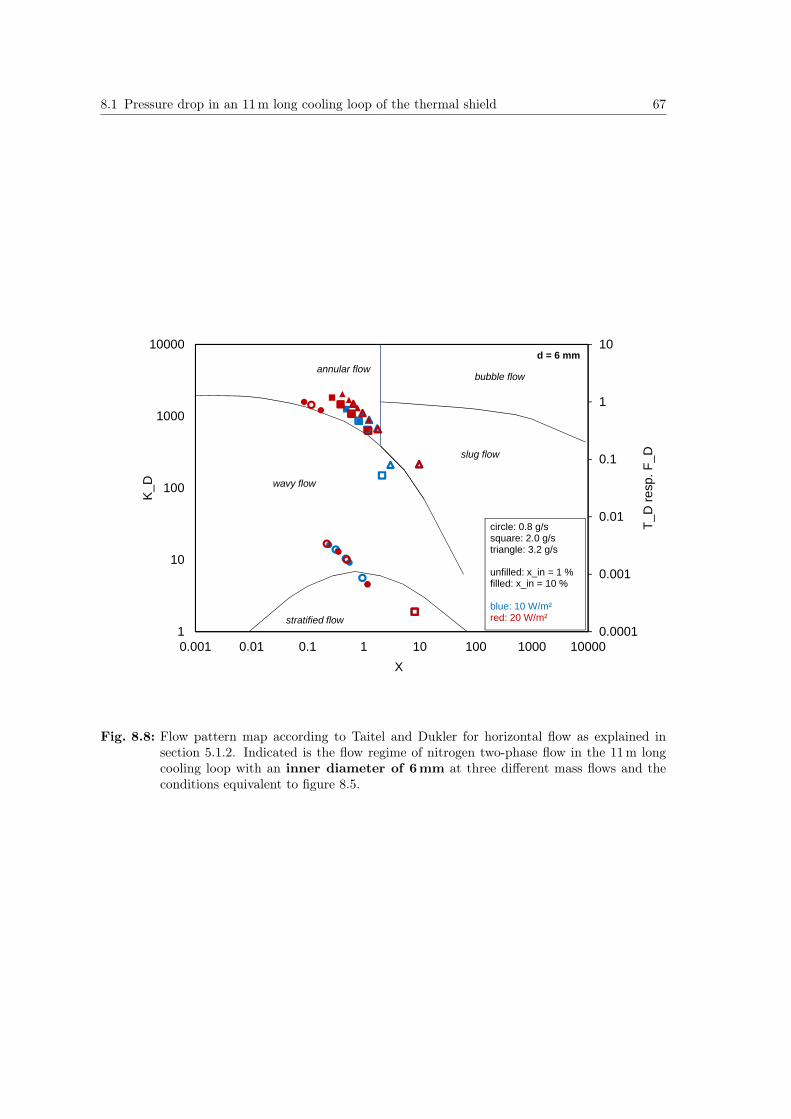
8.1 Pressure drop in an 11m long cooling loop of the thermal shield 67
0.0001
0.001
0.01
0.1
1
10
1
10
100
1000
10000
0.001 0.01 0.1 1 10 100 1000 10000T_
D re
sp. F
_D
K_D
X
slug flow
annular flowbubble flow
wavy flow
stratified flow
circle: 0.8 g/ssquare: 2.0 g/striangle: 3.2 g/s
unfilled: x_in = 1 %filled: x_in = 10 %
blue: 10 W/m²red: 20 W/m²
d = 6 mm
Fig. 8.8: Flow pattern map according to Taitel and Dukler for horizontal flow as explained insection 5.1.2. Indicated is the flow regime of nitrogen two-phase flow in the 11m longcooling loop with an inner diameter of 6mm at three different mass flows and theconditions equivalent to figure 8.5.
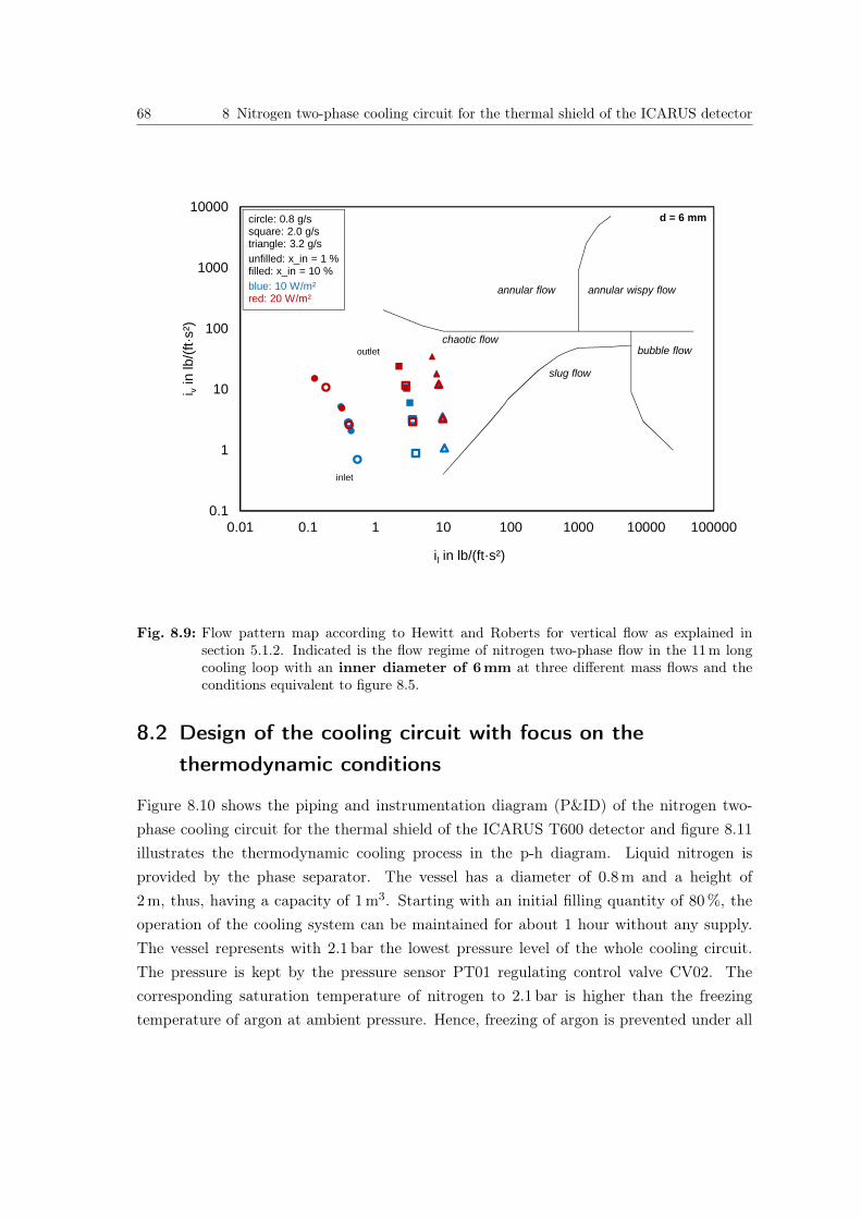
68 8 Nitrogen two-phase cooling circuit for the thermal shield of the ICARUS detector
0.1
1
10
100
1000
10000
0.01 0.1 1 10 100 1000 10000 100000
i vin
lb/(f
t·s²)
il in lb/(ft·s²)
annular flow annular wispy flow
chaotic flow
slug flow
bubble flow
inlet
outlet
circle: 0.8 g/ssquare: 2.0 g/striangle: 3.2 g/sunfilled: x_in = 1 %filled: x_in = 10 %blue: 10 W/m²red: 20 W/m²
d = 6 mm
Fig. 8.9: Flow pattern map according to Hewitt and Roberts for vertical flow as explained insection 5.1.2. Indicated is the flow regime of nitrogen two-phase flow in the 11m longcooling loop with an inner diameter of 6mm at three different mass flows and theconditions equivalent to figure 8.5.
8.2 Design of the cooling circuit with focus on thethermodynamic conditions
Figure 8.10 shows the piping and instrumentation diagram (P&ID) of the nitrogen two-phase cooling circuit for the thermal shield of the ICARUS T600 detector and figure 8.11illustrates the thermodynamic cooling process in the p-h diagram. Liquid nitrogen isprovided by the phase separator. The vessel has a diameter of 0.8 m and a height of2 m, thus, having a capacity of 1 m3. Starting with an initial filling quantity of 80 %, theoperation of the cooling system can be maintained for about 1 hour without any supply.The vessel represents with 2.1 bar the lowest pressure level of the whole cooling circuit.The pressure is kept by the pressure sensor PT01 regulating control valve CV02. Thecorresponding saturation temperature of nitrogen to 2.1 bar is higher than the freezingtemperature of argon at ambient pressure. Hence, freezing of argon is prevented under all
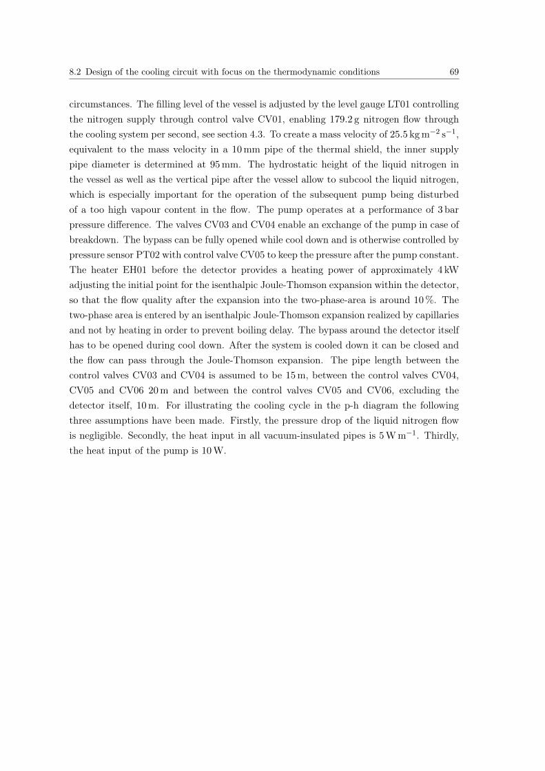
8.2 Design of the cooling circuit with focus on the thermodynamic conditions 69
circumstances. The filling level of the vessel is adjusted by the level gauge LT01 controllingthe nitrogen supply through control valve CV01, enabling 179.2 g nitrogen flow throughthe cooling system per second, see section 4.3. To create a mass velocity of 25.5 kg m−2 s−1,equivalent to the mass velocity in a 10 mm pipe of the thermal shield, the inner supplypipe diameter is determined at 95 mm. The hydrostatic height of the liquid nitrogen inthe vessel as well as the vertical pipe after the vessel allow to subcool the liquid nitrogen,which is especially important for the operation of the subsequent pump being disturbedof a too high vapour content in the flow. The pump operates at a performance of 3 bar
pressure difference. The valves CV03 and CV04 enable an exchange of the pump in case ofbreakdown. The bypass can be fully opened while cool down and is otherwise controlled bypressure sensor PT02 with control valve CV05 to keep the pressure after the pump constant.The heater EH01 before the detector provides a heating power of approximately 4 kWadjusting the initial point for the isenthalpic Joule-Thomson expansion within the detector,so that the flow quality after the expansion into the two-phase-area is around 10 %. Thetwo-phase area is entered by an isenthalpic Joule-Thomson expansion realized by capillariesand not by heating in order to prevent boiling delay. The bypass around the detector itselfhas to be opened during cool down. After the system is cooled down it can be closed andthe flow can pass through the Joule-Thomson expansion. The pipe length between thecontrol valves CV03 and CV04 is assumed to be 15 m, between the control valves CV04,CV05 and CV06 20 m and between the control valves CV05 and CV06, excluding thedetector itself, 10 m. For illustrating the cooling cycle in the p-h diagram the followingthree assumptions have been made. Firstly, the pressure drop of the liquid nitrogen flowis negligible. Secondly, the heat input in all vacuum-insulated pipes is 5 W m−1. Thirdly,the heat input of the pump is 10 W.
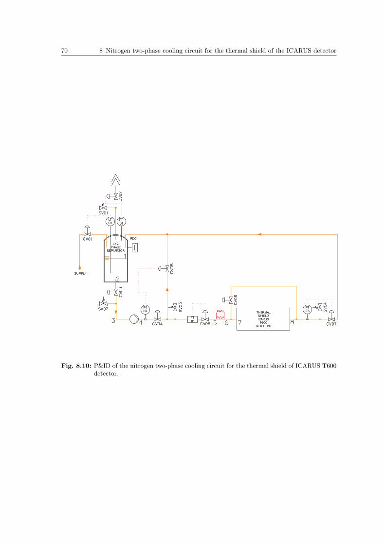
70 8 Nitrogen two-phase cooling circuit for the thermal shield of the ICARUS detector
Fig. 8.10: P&ID of the nitrogen two-phase cooling circuit for the thermal shield of ICARUS T600detector.
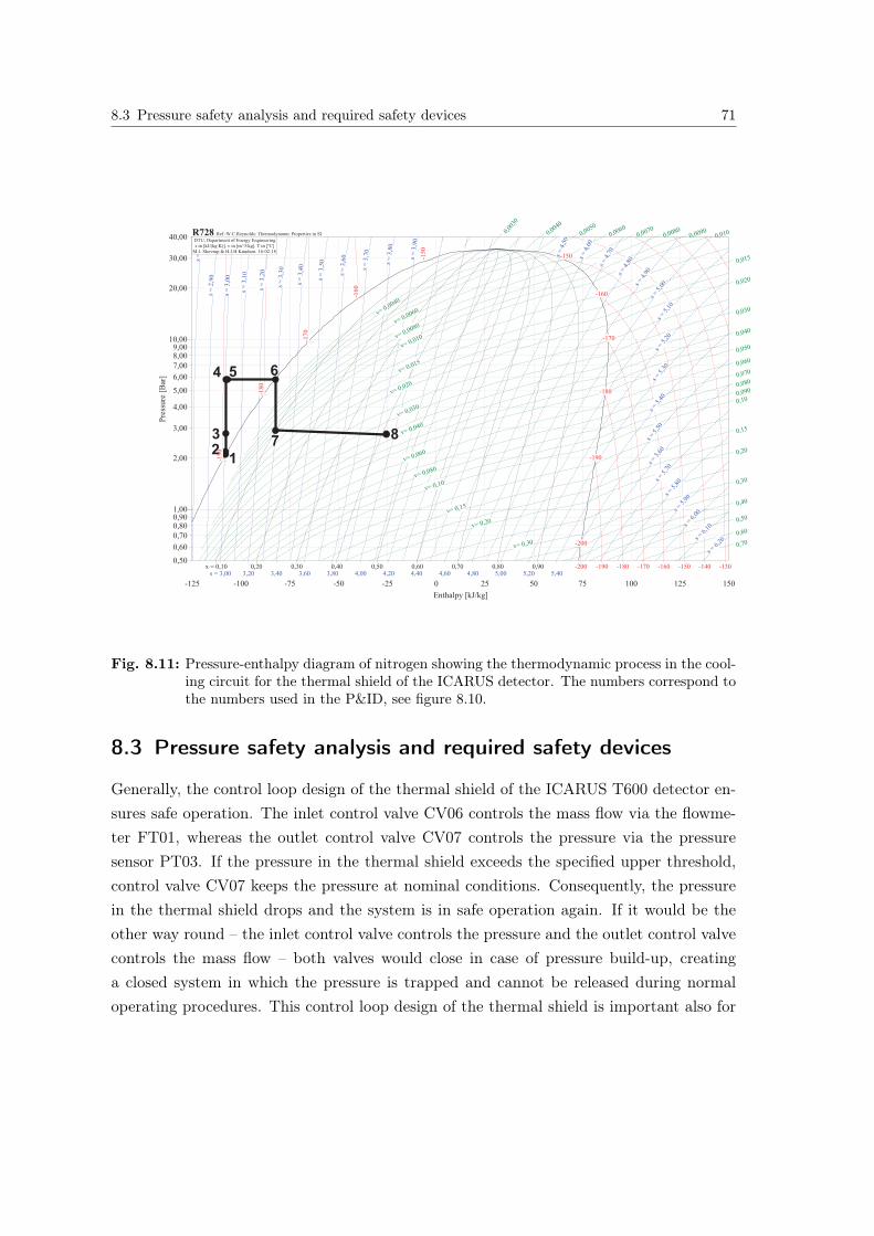
8.3 Pressure safety analysis and required safety devices 71
���������� ���
���� ���� ��� ��� ��� � �� �� �� ��� ��� ���
������������
����
����
����
����������������
����
���
!���
����
����
����
��������
�����
�����
����
!����
�"!���
�"!���
�"!���
�"!���
�"!���
�"����
�"����
�"����
�"�� �
�"��!�
�"����
�"����
�"����
�"����
�"����
�"����
�"����
�"����
�"����
�"����
�" ���
�" � ��
�" ���
�" � �
�" �!�
�" ���
�" ���
�" ���
�" ���
�" ���
����
����
����
����
����
����
����
����
����
����
����
����
��!� �� �
����
����
����
����
����
���� �
����!�
������
������
������
������
������
�����
�����
�����
��� �
���!�
�����
�����
�����
�����
�����
����
����
����
�� �
��!�
����
����
����
#"���� ���� �� � ��!� ���� ���� ���� ���� �����" ��� ��� �!� ��� ��� !��� !��� !�!� !��� !��� ���� ���� ��!�
$"����!�
$"���
���
$"���
���
$"���
��
$"���
��
$"���
��
$"���
�
$"���!�
$"�����
$"�����
$"����
$"����
$"����
$"�� �
%&'�%�����(���)*���������+����+��
�+��� ,��-.�/$+�(0 ���/&+�12�
3/�/4�)$���56/�/6-��7���/��������
���� 8�*9:/2/8���)�7�9&���()7���(+;��)����+��+�4<
12
3
4 5 6
78
Fig. 8.11: Pressure-enthalpy diagram of nitrogen showing the thermodynamic process in the cool-ing circuit for the thermal shield of the ICARUS detector. The numbers correspond tothe numbers used in the P&ID, see figure 8.10.
8.3 Pressure safety analysis and required safety devices
Generally, the control loop design of the thermal shield of the ICARUS T600 detector en-sures safe operation. The inlet control valve CV06 controls the mass flow via the flowme-ter FT01, whereas the outlet control valve CV07 controls the pressure via the pressuresensor PT03. If the pressure in the thermal shield exceeds the specified upper threshold,control valve CV07 keeps the pressure at nominal conditions. Consequently, the pressurein the thermal shield drops and the system is in safe operation again. If it would be theother way round – the inlet control valve controls the pressure and the outlet control valvecontrols the mass flow – both valves would close in case of pressure build-up, creatinga closed system in which the pressure is trapped and cannot be released during normaloperating procedures. This control loop design of the thermal shield is important also for
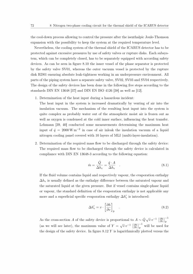
72 8 Nitrogen two-phase cooling circuit for the thermal shield of the ICARUS detector
the cool-down process allowing to control the pressure after the isenthalpic Joule-Thomsonexpansion with the possibility to keep the system at the required temperature level.Nevertheless, the cooling system of the thermal shield of the ICARUS detector has to be
protected against excessive pressures by use of safety valves or rupture disks. Each subsys-tem, which can be completely closed, has to be separately equipped with according safetydevices. As can be seen in figure 8.10 the inner vessel of the phase separator is protectedby the safety valve SV01, whereas the outer vacuum vessel is protected by the rupturedisk RD01 ensuring absolute leak-tightness working in an underpressure environment. Allparts of the piping system have a separate safety valve, SV02, SV03 and SV04 respectively.The design of the safety devices has been done in the following five steps according to thestandards DIN EN 13648 [37] and DIN EN ISO 4126 [38] as well as [12].
1. Determination of the heat input during a hazardous incident:The heat input in the system is increased dramatically by venting of air into theinsulation vacuum. The mechanism of the resulting heat input into the system isquite complex as probably water out of the atmospheric moist air is frozen out aswell as oxygen is condensed at the cold inner surface, influencing the heat transfer.Lehmann [39, 40] conducted some measurements determining the maximum heatinput of q = 2000 W m−2 in case of air inleak the insulation vacuum of a liquidnitrogen cooling panel covered with 10 layers of MLI (multi-layer-insulation).
2. Determination of the required mass flow to be discharged through the safety device:The required mass flow to be discharged through the safety device is calculated incompliance with DIN EN 13648-3 according to the following equation:
m =Q
∆hv=q ·A∆hv
. (8.1)
If the fluid volume contains liquid and respectively vapour, the evaporation enthalpy∆hv is usually defined as the enthalpy difference between the saturated vapour andthe saturated liquid at the given pressure. But if vessel contains single-phase liquidor vapour, the standard definition of the evaporation enthalpy is not applicable anymore and a superficial specific evaporation enthalpy ∆h′v is introduced:
∆h′v = v ·[∂h
∂v
]p
. (8.2)
As the cross-section A of the safety device is proportional to A ∼ Q√v v−1
[∂h∂v
]−1
p
(as we will see later), the maximum value of Y =√v v−1
[∂h∂v
]−1
pwill be used for
the design of the safety device. In figure 8.12 Y is logarithmically plotted versus the
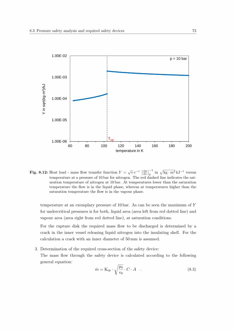
8.3 Pressure safety analysis and required safety devices 73
1.00E-06
1.00E-05
1.00E-04
1.00E-03
1.00E-02
60 80 100 120 140 160 180 200
Y in
sqr
t(kg·
m³)
/kJ
temperature in K
p = 10 bar
Tsat
Fig. 8.12: Heat load - mass flow transfer function Y =√v v−1
[∂h∂v
]−1
pin√
kg ·m3 kJ−1 versustemperature at a pressure of 10 bar for nitrogen. The red dashed line indicates the sat-uration temperature of nitrogen at 10 bar. At temperatures lower than the saturationtemperature the flow is in the liquid phase, whereas at temperatures higher than thesaturation temperature the flow is in the vapour phase.
temperature at an exemplary pressure of 10 bar. As can be seen the maximum of Yfor undercritical pressures is for both, liquid area (area left from red dotted line) andvapour area (area right from red dotted line), at saturation conditions.
For the rupture disk the required mass flow to be discharged is determined by acrack in the inner vessel releasing liquid nitrogen into the insulating shell. For thecalculation a crack with an inner diameter of 50 mm is assumed.
3. Determination of the required cross-section of the safety device:The mass flow through the safety device is calculated according to the followinggeneral equation:
m = Kdr ·√p0
v0· C ·A . (8.3)
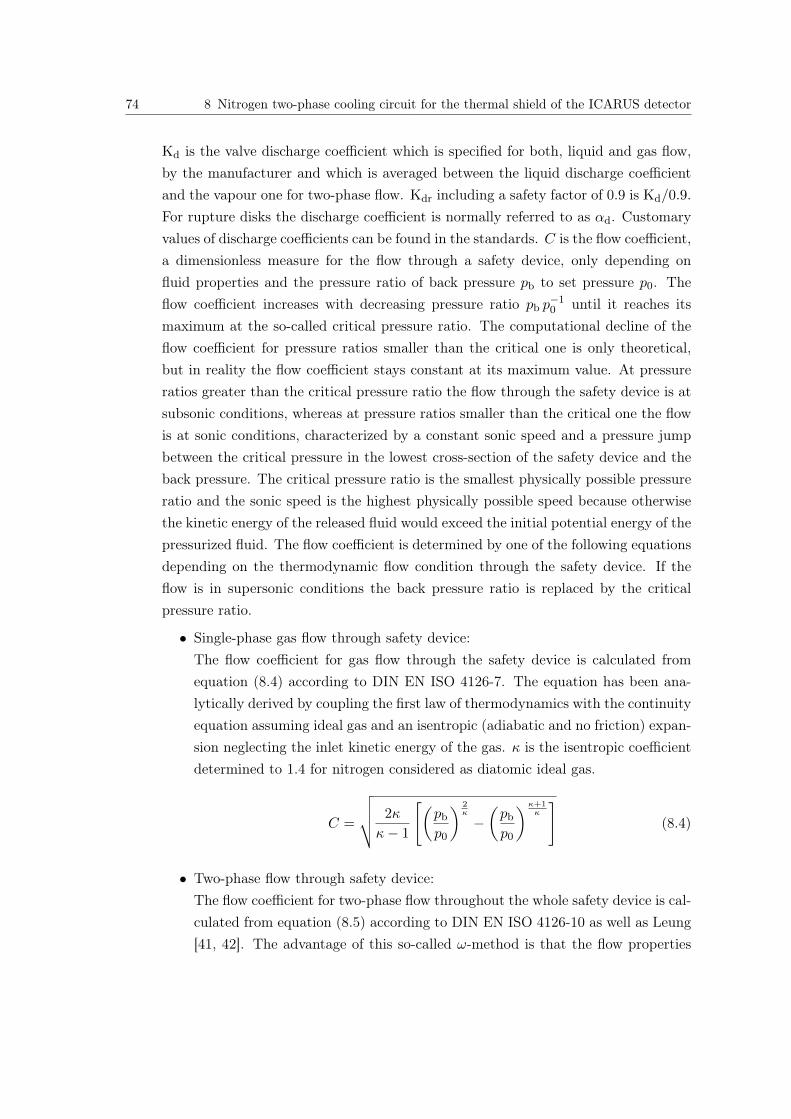
74 8 Nitrogen two-phase cooling circuit for the thermal shield of the ICARUS detector
Kd is the valve discharge coefficient which is specified for both, liquid and gas flow,by the manufacturer and which is averaged between the liquid discharge coefficientand the vapour one for two-phase flow. Kdr including a safety factor of 0.9 is Kd/0.9.For rupture disks the discharge coefficient is normally referred to as αd. Customaryvalues of discharge coefficients can be found in the standards. C is the flow coefficient,a dimensionless measure for the flow through a safety device, only depending onfluid properties and the pressure ratio of back pressure pb to set pressure p0. Theflow coefficient increases with decreasing pressure ratio pb p
−10 until it reaches its
maximum at the so-called critical pressure ratio. The computational decline of theflow coefficient for pressure ratios smaller than the critical one is only theoretical,but in reality the flow coefficient stays constant at its maximum value. At pressureratios greater than the critical pressure ratio the flow through the safety device is atsubsonic conditions, whereas at pressure ratios smaller than the critical one the flowis at sonic conditions, characterized by a constant sonic speed and a pressure jumpbetween the critical pressure in the lowest cross-section of the safety device and theback pressure. The critical pressure ratio is the smallest physically possible pressureratio and the sonic speed is the highest physically possible speed because otherwisethe kinetic energy of the released fluid would exceed the initial potential energy of thepressurized fluid. The flow coefficient is determined by one of the following equationsdepending on the thermodynamic flow condition through the safety device. If theflow is in supersonic conditions the back pressure ratio is replaced by the criticalpressure ratio.
• Single-phase gas flow through safety device:The flow coefficient for gas flow through the safety device is calculated fromequation (8.4) according to DIN EN ISO 4126-7. The equation has been ana-lytically derived by coupling the first law of thermodynamics with the continuityequation assuming ideal gas and an isentropic (adiabatic and no friction) expan-sion neglecting the inlet kinetic energy of the gas. κ is the isentropic coefficientdetermined to 1.4 for nitrogen considered as diatomic ideal gas.
C =
√√√√ 2κ
κ− 1
[(pb
p0
) 2κ
−(pb
p0
)κ+1κ
](8.4)
• Two-phase flow through safety device:The flow coefficient for two-phase flow throughout the whole safety device is cal-culated from equation (8.5) according to DIN EN ISO 4126-10 as well as Leung[41, 42]. The advantage of this so-called ω-method is that the flow properties
8.3 Pressure safety analysis and required safety devices 75
at the entrance of the safety device, which are easily accessible, are used. Itassumes a frictionless flow, no heat transfer to the surroundings and mechanicalequilibrium, that means no slip between the two phases. The parameter ω takesthe compressibility of the two-phase flow into account. The first term of equa-tion (8.6) describes the compressibility of the flow due to the vapour volumeand the second term reflects the compressibility due to phase change occurringduring depressurization. The factor N , see equation (8.7), is the boiling-delayfactor taking into account that the flow might not be in thermodynamic equi-librium, which becomes more probable with increasing pressure difference overthe valve. The parameter ωeq assumes homogeneous two-phase equilibrium,this means N = 1. At constant set pressure p0 and constant back pressure pbbut variable inlet flow quality x0, the critical pressure ratio is decreasing withincreasing flow quality approaching the value of the critical pressure ratio of thegas flow at x0 = 1.
C =
√2[ω · ln
(p0pb
)− (ω − 1)
(1− pb
p0
)]ω(p0pb− 1)
+ 1(8.5)
ω =x0 · vv0
κ · v0+cpl0 · T0 · p0
v0
(vv0 − vl0
∆hv0
)2
·N (8.6)
N =
(x0 + cpl0 · p0 · T0 ·
vv0 − vl0
∆hv02 · ln
(p0
pb
)) 25
(8.7)
• Initially subcooled liquid potentially evaporating in safety device:The flow coefficient for initially subcooled flow throughout the safety device iscalculated from equation (8.11) according to Schmidt [43], to which DIN EN ISO4126-10 is referring to. The approach of Schmidt is an extension of the ω-modelfor two-phase flow. The model of Schmidt distinguishes between three differentcases introducing the following three pressure ratios
ηb = pb p−10 (8.8)
ηsat = psat p−10 (8.9)
ηcrit = pcrit p−10 . (8.10)
76 8 Nitrogen two-phase cooling circuit for the thermal shield of the ICARUS detector
If the flow is subsonic, η = ηb in the following equations and the safety de-vice is divided into a flow region with liquid flow up to psat and a subsequentflow region with two-phase flow from psat to pb. If the flow is supersonic andwas initially slightly subcooled so that pcrit < psat, η = ηcrit in the followingequations. If the flow is supersonic and was initially highly subcooled so thatpcrit > psat, η = ηsat in the following equations, the equation (8.11) simplifies toequation (8.14). At constant set pressure p0 and constant back pressure pb butvariable inlet subcooling, the critical pressure ratio increases with decreasinginitial subcooling.
C =
√2 · (1− ηsat) + 2 ·
[ω · ηsat · ln
(ηsatη
)− (ω − 1) (ηsat − η)
]ω(ηsatη − 1
)+ 1
(8.11)
ω =x0 · vv0
κ · v0+cpl0 · T0 · p0 · ηsat
v0
(vv0 − vl0
∆hv0
)2
·N (8.12)
N =
(x0 + cpl0 · p0 · T0 · ηsat ·
vv0 − vl0
∆hv02 · ln
(ηsat
η
))η−0.6sat
(8.13)
C =√
2 · (1− ηsat) (8.14)
4. Sizing inlet piping:The pressure drop of the safety valve inlet pipe has to be smaller than 3 % of the gaugeset pressure of the safety valve according to DIN EN 13648-3 and DIN EN ISO 4126-9.Otherwise the big pressure loss in the inlet pipe can result in some negative dynamiceffects leading to an unstable operation of the safety valve. High frequency vibrations,causing the safety valve to open and close quickly, so-called chattering, drasticallyreduce its lifetime. The additional heat load of the inlet pipe has only to be consideredfor design if the inlet pipe exceeds a length of 0.6 m. For the four safety valves SV01to SV04 the maximum pressure drop of the inlet pipe is reasonably estimated by thefollowing equation:
∆p =
(fin + fp ·
L
d
)· 0.5 · ρ · u2 =
(fin + fp ·
L
d
)· 0.5 · v · m
2
A2. (8.15)
The friction factor fin is assumed to be 0.5 for a very sharp angular inlet and the fric-tion factor fp is approximated as a constant of 0.05, not dependent on the Reynolds
8.3 Pressure safety analysis and required safety devices 77
number and the roughness of the wall. For two-phase flow in the inlet pipe thepressure drop is multiplied by a safety coefficient of two.
For rupture disks the pressure drop of the inlet pipe does not need to be checked asrupture disks do not create a resonant system.
5. Sizing outlet piping:For the present safety devices there exist no outlet pipes as the nitrogen is directlydischarged into the surrounding environment in case of a hazardous event. Due tothe risk of oxygen deficiency it is necessary to install an oxygen monitoring systemin the laboratory halls including an alarm and evacuation system. Ventilation of thelaboratory halls must be possible.
The p-h diagram, see figure 8.13, illustrates the thermodynamic transformation of thefluid for all safety devices. Until the opening of the safety device the thermodynamictransformation of the system can be described as an isochoric transformation, whereasafter actuating of the safety device the thermodynamic transformation is isobaric (blacklines). The expansion through the safety device itself is approximated by an isenthalpicexpansion (black dotted lines for exemplary inlet conditions on the dewing point curve).It is important to emphasize that due to the further heat input after opening of the safetydevice the inlet conditions of the safety device change; the system can shift isobariclystarting from subcooled liquid through the two-phase area to superheated vapour. Butcalculations for all safety devices prove that for inlet conditions exactly on the dewingpoint curve the generated mass flow to be discharged is the greatest. Consequently, allsafety devices have to be designed for that case. Table 8.1 shows this fact exemplary forsafety valve SV03 with a set pressure of 10 bar. The design of all safety devices at thecritical inlet conditions on the dewing point curve are compiled in table 8.2.
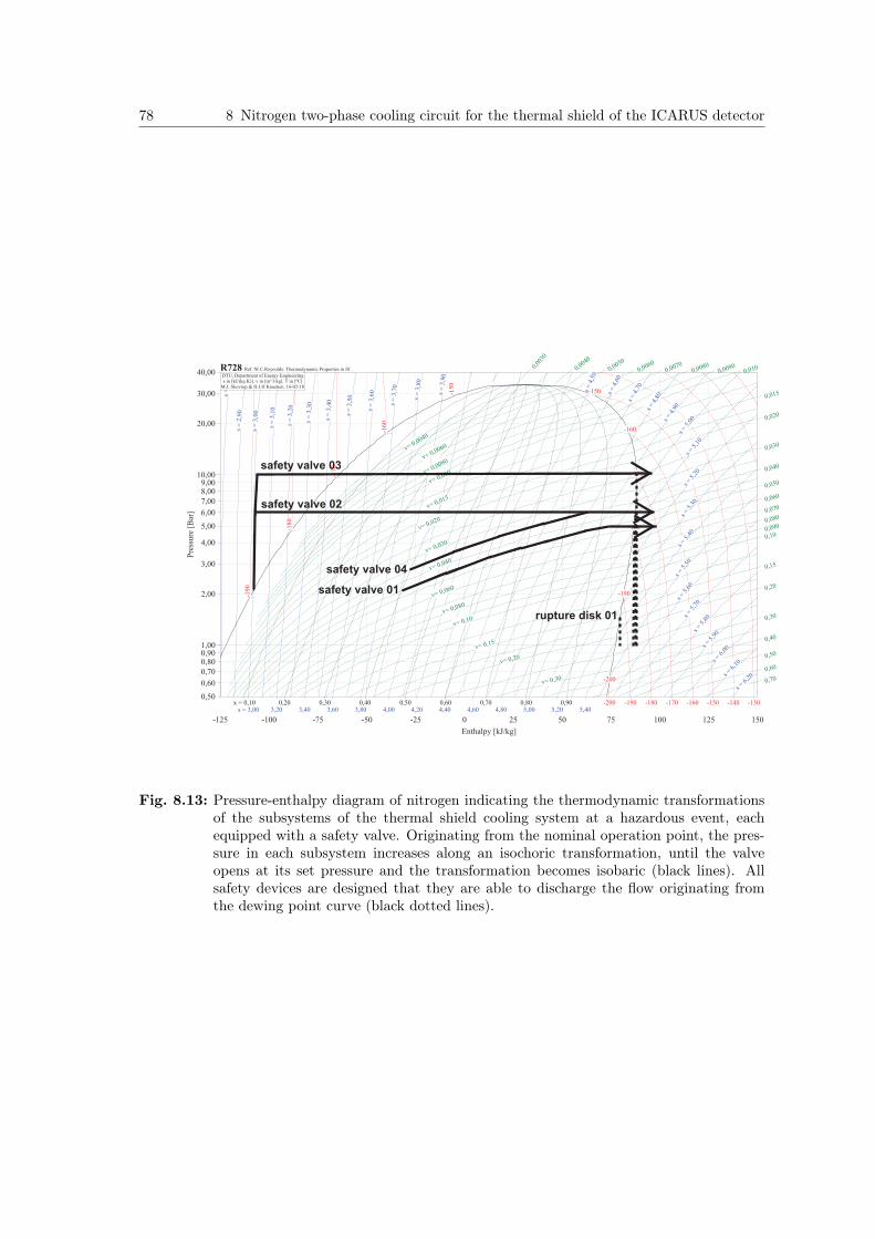
78 8 Nitrogen two-phase cooling circuit for the thermal shield of the ICARUS detector
���������� ���
���� ���� ��� ��� ��� � �� �� �� ��� ��� ���
������������
����
����
����
����������������
����
���
!���
����
����
����
��������
�����
�����
����
!����
�"!���
�"!���
�"!���
�"!���
�"!���
�"����
�"����
�"����
�"�� �
�"��!�
�"����
�"����
�"����
�"����
�"����
�"����
�"����
�"����
�"����
�"����
�" ���
�" � ��
�" ���
�" � �
�" �!�
�" ���
�" ���
�" ���
�" ���
�" ���
����
����
����
����
����
����
����
����
����
����
����
����
��!� �� �
����
����
����
����
����
���� �
����!�
������
������
������
������
������
�����
�����
�����
��� �
���!�
�����
�����
�����
�����
�����
����
����
����
�� �
��!�
����
����
����
#"���� ���� �� � ��!� ���� ���� ���� ���� �����" ��� ��� �!� ��� ��� !��� !��� !�!� !��� !��� ���� ���� ��!�
$"����!�
$"���
���
$"���
���
$"���
��
$"���
��
$"���
��
$"���
�
$"���!�
$"�����
$"�����
$"����
$"����
$"����
$"�� �
%&'�%�����(���)*���������+����+��
�+��� ,��-.�/$+�(0 ���/&+�12�
3/�/4�)$���56/�/6-��7���/��������
���� 8�*9:/2/8���)�7�9&���()7���(+;��)����+��+�4<
safety valve 01
safety valve 02
safety valve 03
safety valve 04
rupture disk 01
Fig. 8.13: Pressure-enthalpy diagram of nitrogen indicating the thermodynamic transformationsof the subsystems of the thermal shield cooling system at a hazardous event, eachequipped with a safety valve. Originating from the nominal operation point, the pres-sure in each subsystem increases along an isochoric transformation, until the valveopens at its set pressure and the transformation becomes isobaric (black lines). Allsafety devices are designed that they are able to discharge the flow originating fromthe dewing point curve (black dotted lines).
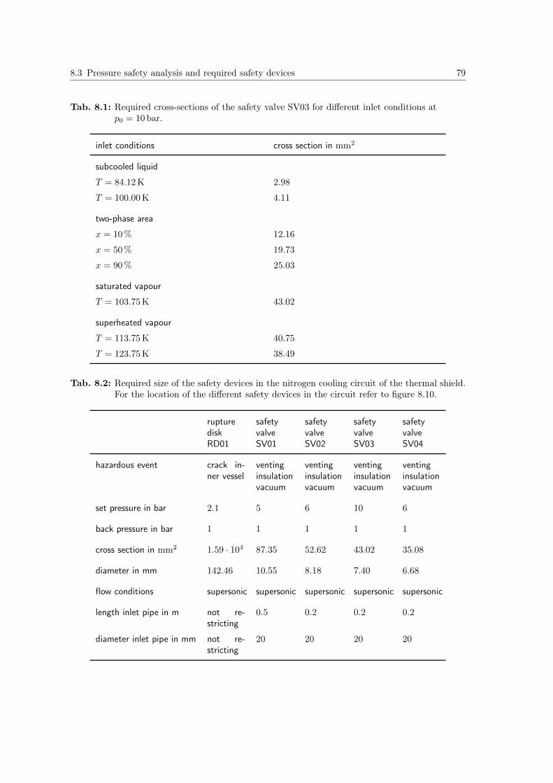
8.3 Pressure safety analysis and required safety devices 79
Tab. 8.1: Required cross-sections of the safety valve SV03 for different inlet conditions atp0 = 10 bar.
inlet conditions cross section in mm2
subcooled liquid
T = 84.12 K 2.98
T = 100.00 K 4.11
two-phase area
x = 10 % 12.16
x = 50 % 19.73
x = 90 % 25.03
saturated vapour
T = 103.75 K 43.02
superheated vapour
T = 113.75 K 40.75
T = 123.75 K 38.49
Tab. 8.2: Required size of the safety devices in the nitrogen cooling circuit of the thermal shield.For the location of the different safety devices in the circuit refer to figure 8.10.
rupturediskRD01
safetyvalveSV01
safetyvalveSV02
safetyvalveSV03
safetyvalveSV04
hazardous event crack in-ner vessel
ventinginsulationvacuum
ventinginsulationvacuum
ventinginsulationvacuum
ventinginsulationvacuum
set pressure in bar 2.1 5 6 10 6
back pressure in bar 1 1 1 1 1
cross section in mm2 1.59 · 104 87.35 52.62 43.02 35.08
diameter in mm 142.46 10.55 8.18 7.40 6.68
flow conditions supersonic supersonic supersonic supersonic supersonic
length inlet pipe in m not re-stricting
0.5 0.2 0.2 0.2
diameter inlet pipe in mm not re-stricting
20 20 20 20
9 Conclusion
The large-scale ICARUS T600 detector is designed to detect neutrinos allowing researchin the field of neutrino oscillations. Is will be filled with liquid argon and operate atambient pressure. Consequently, its operation temperature is determined at 87 K, thesaturation temperature of argon at ambient pressure. For studying the interactions betweenneutrinos and argon atoms as precisely as possible, temperature gradients and the resultingconvection of the liquid argon inside the detector has to be minimized. Hence, the detectoris equipped with a thermal shield, which is actively cooled with boiling nitrogen at the sametemperature as the detector. It operates at a pressure of 2.8 bar, which is the saturationpressure of nitrogen at 87 K. The thermal shield should be able to absorb an outer heatflux of 20 W m−2 and should have a temperature gradient less than 500 mK. Theoretically,not considering the pressure drop along the cooling circuit, the temperature stays constantduring evaporation in the chosen two-phase flow regime. The only temperature change iscaused by the small pressure drop along the cooling loop. Due to the strict temperatureconstraints, it is important to study the pressure drop of the nitrogen two-phase flow alongthe cooling circuit of the thermal shield in different orientations of the flow in respect togravity.An overview of the existing literature of two-phase flow has been given. Characteristic
properties of two-phase flow are the flow quality, the void fraction and the flow pattern.The first two properties quantify the proportion of the vapour phase to the total flow.The latter describes the distribution of the two phases at the cross-section of the pipe.The total pressure drop of two-phase flow is the sum of the gravitational, frictional andmomentum pressure drop. In contrast to the well-known pressure drop in single-phaseliquid or vapour flow, the momentum pressure drop, describing the acceleration of theflow during evaporation, has to be taken into account for two-phase flow. As most of thecorrelations for the void fraction and the frictional pressure drop of two-phase flow areempirical correlations, it is difficult to utilize them at other conditions they were originallydeveloped for. A lack of a database for the pressure drop of nitrogen two-phase flow at theconditions of the ICARUS thermal shield underlines the need of a further investigation.An experimental setup has been built in order to determine the pressure drop in ni-
trogen two-phase flow in a horizontal, vertical upward and vertical downward part. The
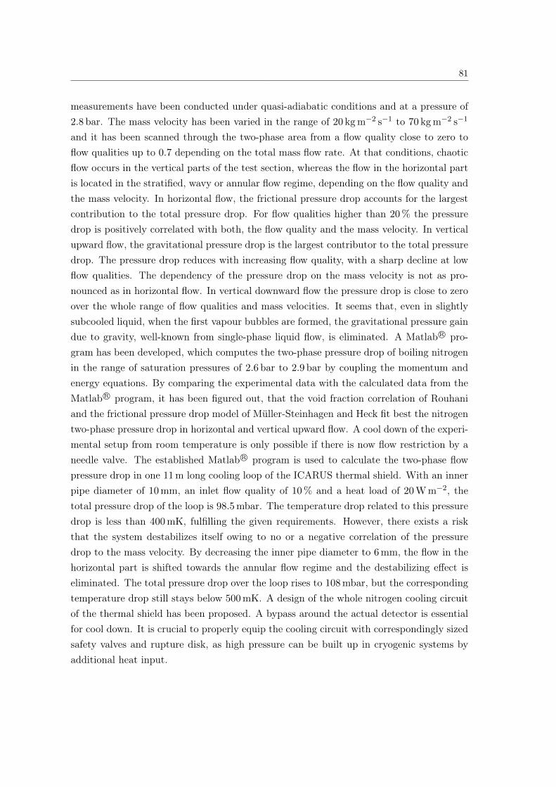
81
measurements have been conducted under quasi-adiabatic conditions and at a pressure of2.8 bar. The mass velocity has been varied in the range of 20 kg m−2 s−1 to 70 kg m−2 s−1
and it has been scanned through the two-phase area from a flow quality close to zero toflow qualities up to 0.7 depending on the total mass flow rate. At that conditions, chaoticflow occurs in the vertical parts of the test section, whereas the flow in the horizontal partis located in the stratified, wavy or annular flow regime, depending on the flow quality andthe mass velocity. In horizontal flow, the frictional pressure drop accounts for the largestcontribution to the total pressure drop. For flow qualities higher than 20 % the pressuredrop is positively correlated with both, the flow quality and the mass velocity. In verticalupward flow, the gravitational pressure drop is the largest contributor to the total pressuredrop. The pressure drop reduces with increasing flow quality, with a sharp decline at lowflow qualities. The dependency of the pressure drop on the mass velocity is not as pro-nounced as in horizontal flow. In vertical downward flow the pressure drop is close to zeroover the whole range of flow qualities and mass velocities. It seems that, even in slightlysubcooled liquid, when the first vapour bubbles are formed, the gravitational pressure gaindue to gravity, well-known from single-phase liquid flow, is eliminated. A Matlab R© pro-gram has been developed, which computes the two-phase pressure drop of boiling nitrogenin the range of saturation pressures of 2.6 bar to 2.9 bar by coupling the momentum andenergy equations. By comparing the experimental data with the calculated data from theMatlab R© program, it has been figured out, that the void fraction correlation of Rouhaniand the frictional pressure drop model of Müller-Steinhagen and Heck fit best the nitrogentwo-phase pressure drop in horizontal and vertical upward flow. A cool down of the experi-mental setup from room temperature is only possible if there is now flow restriction by aneedle valve. The established Matlab R© program is used to calculate the two-phase flowpressure drop in one 11 m long cooling loop of the ICARUS thermal shield. With an innerpipe diameter of 10 mm, an inlet flow quality of 10 % and a heat load of 20 W m−2, thetotal pressure drop of the loop is 98.5 mbar. The temperature drop related to this pressuredrop is less than 400 mK, fulfilling the given requirements. However, there exists a riskthat the system destabilizes itself owing to no or a negative correlation of the pressuredrop to the mass velocity. By decreasing the inner pipe diameter to 6 mm, the flow in thehorizontal part is shifted towards the annular flow regime and the destabilizing effect iseliminated. The total pressure drop over the loop rises to 108 mbar, but the correspondingtemperature drop still stays below 500 mK. A design of the whole nitrogen cooling circuitof the thermal shield has been proposed. A bypass around the actual detector is essentialfor cool down. It is crucial to properly equip the cooling circuit with correspondingly sizedsafety valves and rupture disk, as high pressure can be built up in cryogenic systems byadditional heat input.
List of Tables
Tab. 7.1 Accuracy specifications of the used measuring instruments according to the manufacturers.The letters A to E refer to the individual measuring instruments as listed. . . . . . . . . . 38
Tab. 7.2 Maximum error of the flow quality at four different measurement points: low and high massflow and low and high flow quality. . . . . . . . . . . . . . . . . . . . . . . . . . . . . . . . . 41
Tab. 7.3 Mass flow and mass velocity values of the nine measurements. The pipe of the test sectionhas an inner diameter of 6mm. . . . . . . . . . . . . . . . . . . . . . . . . . . . . . . . . . . 42
Tab. 8.1 Required cross-sections of the safety valve SV03 for different inlet conditions at p0 = 10bar. 79Tab. 8.2 Required size of the safety devices in the nitrogen cooling circuit of the thermal shield. For
the location of the different safety devices in the circuit refer to figure 8.10. . . . . . . . . . 79
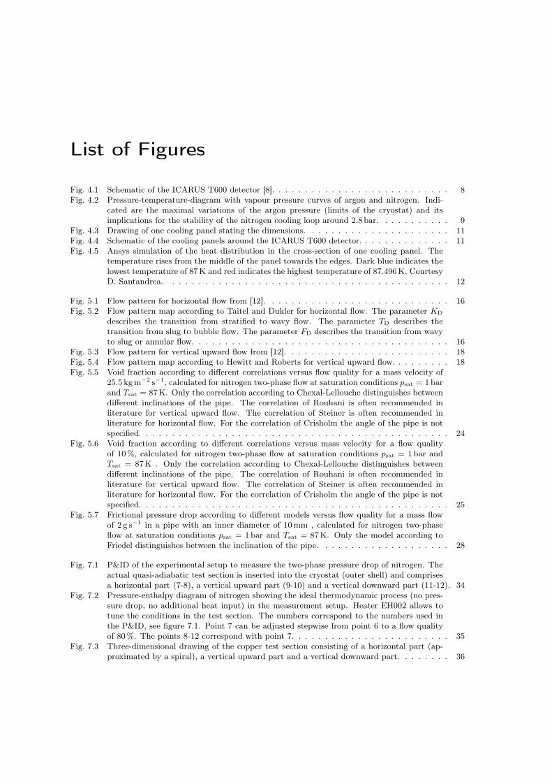
List of Figures
Fig. 4.1 Schematic of the ICARUS T600 detector [8]. . . . . . . . . . . . . . . . . . . . . . . . . . . 8Fig. 4.2 Pressure-temperature-diagram with vapour pressure curves of argon and nitrogen. Indi-
cated are the maximal variations of the argon pressure (limits of the cryostat) and itsimplications for the stability of the nitrogen cooling loop around 2.8 bar. . . . . . . . . . . 9
Fig. 4.3 Drawing of one cooling panel stating the dimensions. . . . . . . . . . . . . . . . . . . . . . 11Fig. 4.4 Schematic of the cooling panels around the ICARUS T600 detector. . . . . . . . . . . . . . 11Fig. 4.5 Ansys simulation of the heat distribution in the cross-section of one cooling panel. The
temperature rises from the middle of the panel towards the edges. Dark blue indicates thelowest temperature of 87K and red indicates the highest temperature of 87.496K, CourtesyD. Santandrea. . . . . . . . . . . . . . . . . . . . . . . . . . . . . . . . . . . . . . . . . . . 12
Fig. 5.1 Flow pattern for horizontal flow from [12]. . . . . . . . . . . . . . . . . . . . . . . . . . . . 16Fig. 5.2 Flow pattern map according to Taitel and Dukler for horizontal flow. The parameter KD
describes the transition from stratified to wavy flow. The parameter TD describes thetransition from slug to bubble flow. The parameter FD describes the transition from wavyto slug or annular flow. . . . . . . . . . . . . . . . . . . . . . . . . . . . . . . . . . . . . . . 16
Fig. 5.3 Flow pattern for vertical upward flow from [12]. . . . . . . . . . . . . . . . . . . . . . . . . 18Fig. 5.4 Flow pattern map according to Hewitt and Roberts for vertical upward flow. . . . . . . . . 18Fig. 5.5 Void fraction according to different correlations versus flow quality for a mass velocity of
25.5 kgm−2 s−1, calculated for nitrogen two-phase flow at saturation conditions psat = 1barand Tsat = 87K. Only the correlation according to Chexal-Lellouche distinguishes betweendifferent inclinations of the pipe. The correlation of Rouhani is often recommended inliterature for vertical upward flow. The correlation of Steiner is often recommended inliterature for horizontal flow. For the correlation of Crisholm the angle of the pipe is notspecified. . . . . . . . . . . . . . . . . . . . . . . . . . . . . . . . . . . . . . . . . . . . . . . 24
Fig. 5.6 Void fraction according to different correlations versus mass velocity for a flow qualityof 10%, calculated for nitrogen two-phase flow at saturation conditions psat = 1bar andTsat = 87K . Only the correlation according to Chexal-Lellouche distinguishes betweendifferent inclinations of the pipe. The correlation of Rouhani is often recommended inliterature for vertical upward flow. The correlation of Steiner is often recommended inliterature for horizontal flow. For the correlation of Crisholm the angle of the pipe is notspecified. . . . . . . . . . . . . . . . . . . . . . . . . . . . . . . . . . . . . . . . . . . . . . . 25
Fig. 5.7 Frictional pressure drop according to different models versus flow quality for a mass flowof 2 g s−1 in a pipe with an inner diameter of 10mm , calculated for nitrogen two-phaseflow at saturation conditions psat = 1bar and Tsat = 87K. Only the model according toFriedel distinguishes between the inclination of the pipe. . . . . . . . . . . . . . . . . . . . 28
Fig. 7.1 P&ID of the experimental setup to measure the two-phase pressure drop of nitrogen. Theactual quasi-adiabatic test section is inserted into the cryostat (outer shell) and comprisesa horizontal part (7-8), a vertical upward part (9-10) and a vertical downward part (11-12). 34
Fig. 7.2 Pressure-enthalpy diagram of nitrogen showing the ideal thermodynamic process (no pres-sure drop, no additional heat input) in the measurement setup. Heater EH002 allows totune the conditions in the test section. The numbers correspond to the numbers used inthe P&ID, see figure 7.1. Point 7 can be adjusted stepwise from point 6 to a flow qualityof 80%. The points 8-12 correspond with point 7. . . . . . . . . . . . . . . . . . . . . . . . 35
Fig. 7.3 Three-dimensional drawing of the copper test section consisting of a horizontal part (ap-proximated by a spiral), a vertical upward part and a vertical downward part. . . . . . . . 36
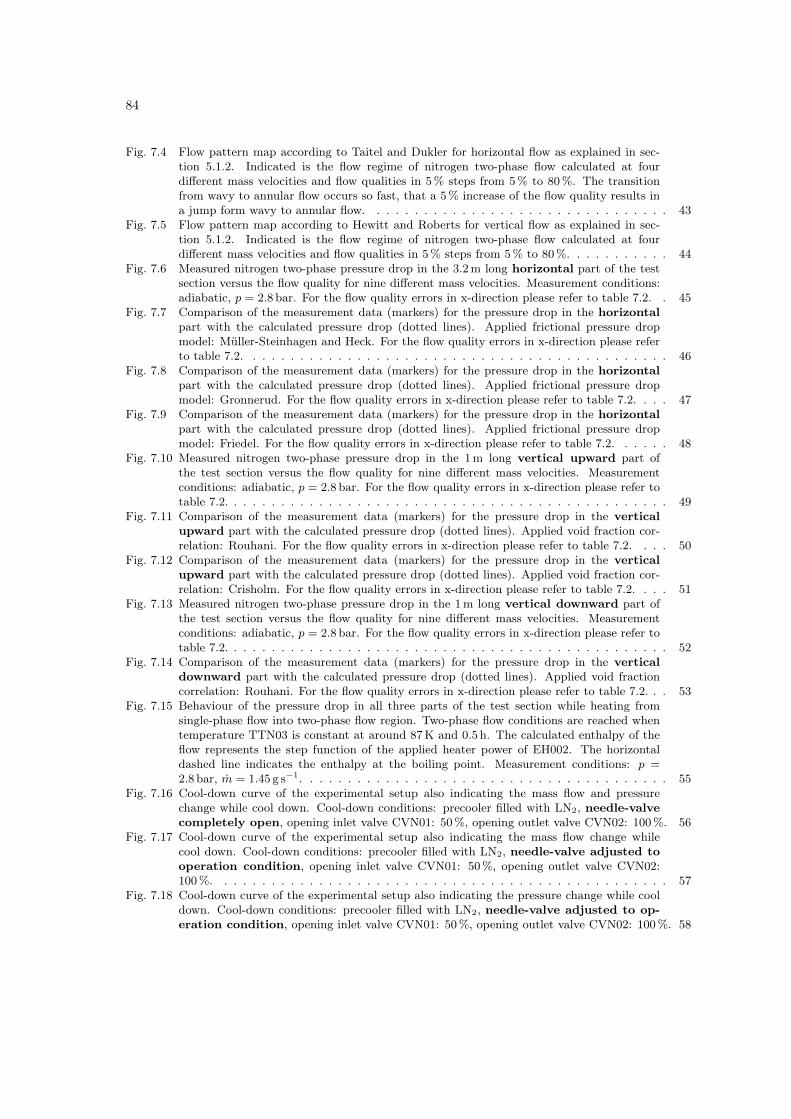
84
Fig. 7.4 Flow pattern map according to Taitel and Dukler for horizontal flow as explained in sec-tion 5.1.2. Indicated is the flow regime of nitrogen two-phase flow calculated at fourdifferent mass velocities and flow qualities in 5% steps from 5% to 80%. The transitionfrom wavy to annular flow occurs so fast, that a 5% increase of the flow quality results ina jump form wavy to annular flow. . . . . . . . . . . . . . . . . . . . . . . . . . . . . . . . 43
Fig. 7.5 Flow pattern map according to Hewitt and Roberts for vertical flow as explained in sec-tion 5.1.2. Indicated is the flow regime of nitrogen two-phase flow calculated at fourdifferent mass velocities and flow qualities in 5% steps from 5% to 80%. . . . . . . . . . . 44
Fig. 7.6 Measured nitrogen two-phase pressure drop in the 3.2m long horizontal part of the testsection versus the flow quality for nine different mass velocities. Measurement conditions:adiabatic, p = 2.8 bar. For the flow quality errors in x-direction please refer to table 7.2. . 45
Fig. 7.7 Comparison of the measurement data (markers) for the pressure drop in the horizontalpart with the calculated pressure drop (dotted lines). Applied frictional pressure dropmodel: Müller-Steinhagen and Heck. For the flow quality errors in x-direction please referto table 7.2. . . . . . . . . . . . . . . . . . . . . . . . . . . . . . . . . . . . . . . . . . . . . 46
Fig. 7.8 Comparison of the measurement data (markers) for the pressure drop in the horizontalpart with the calculated pressure drop (dotted lines). Applied frictional pressure dropmodel: Gronnerud. For the flow quality errors in x-direction please refer to table 7.2. . . . 47
Fig. 7.9 Comparison of the measurement data (markers) for the pressure drop in the horizontalpart with the calculated pressure drop (dotted lines). Applied frictional pressure dropmodel: Friedel. For the flow quality errors in x-direction please refer to table 7.2. . . . . . 48
Fig. 7.10 Measured nitrogen two-phase pressure drop in the 1m long vertical upward part ofthe test section versus the flow quality for nine different mass velocities. Measurementconditions: adiabatic, p = 2.8 bar. For the flow quality errors in x-direction please refer totable 7.2. . . . . . . . . . . . . . . . . . . . . . . . . . . . . . . . . . . . . . . . . . . . . . . 49
Fig. 7.11 Comparison of the measurement data (markers) for the pressure drop in the verticalupward part with the calculated pressure drop (dotted lines). Applied void fraction cor-relation: Rouhani. For the flow quality errors in x-direction please refer to table 7.2. . . . 50
Fig. 7.12 Comparison of the measurement data (markers) for the pressure drop in the verticalupward part with the calculated pressure drop (dotted lines). Applied void fraction cor-relation: Crisholm. For the flow quality errors in x-direction please refer to table 7.2. . . . 51
Fig. 7.13 Measured nitrogen two-phase pressure drop in the 1m long vertical downward part ofthe test section versus the flow quality for nine different mass velocities. Measurementconditions: adiabatic, p = 2.8 bar. For the flow quality errors in x-direction please refer totable 7.2. . . . . . . . . . . . . . . . . . . . . . . . . . . . . . . . . . . . . . . . . . . . . . . 52
Fig. 7.14 Comparison of the measurement data (markers) for the pressure drop in the verticaldownward part with the calculated pressure drop (dotted lines). Applied void fractioncorrelation: Rouhani. For the flow quality errors in x-direction please refer to table 7.2. . . 53
Fig. 7.15 Behaviour of the pressure drop in all three parts of the test section while heating fromsingle-phase flow into two-phase flow region. Two-phase flow conditions are reached whentemperature TTN03 is constant at around 87K and 0.5 h. The calculated enthalpy of theflow represents the step function of the applied heater power of EH002. The horizontaldashed line indicates the enthalpy at the boiling point. Measurement conditions: p =2.8 bar, m = 1.45 g s−1. . . . . . . . . . . . . . . . . . . . . . . . . . . . . . . . . . . . . . . 55
Fig. 7.16 Cool-down curve of the experimental setup also indicating the mass flow and pressurechange while cool down. Cool-down conditions: precooler filled with LN2, needle-valvecompletely open, opening inlet valve CVN01: 50%, opening outlet valve CVN02: 100%. 56
Fig. 7.17 Cool-down curve of the experimental setup also indicating the mass flow change whilecool down. Cool-down conditions: precooler filled with LN2, needle-valve adjusted tooperation condition, opening inlet valve CVN01: 50%, opening outlet valve CVN02:100%. . . . . . . . . . . . . . . . . . . . . . . . . . . . . . . . . . . . . . . . . . . . . . . . 57
Fig. 7.18 Cool-down curve of the experimental setup also indicating the pressure change while cooldown. Cool-down conditions: precooler filled with LN2, needle-valve adjusted to op-eration condition, opening inlet valve CVN01: 50%, opening outlet valve CVN02: 100%. 58
85
Fig. 8.1 Calculated pressure drop and corresponding reduction of the absolute pressure and tem-perature versus the length of the 11m long cooling loop with an inner diameter of 10mm.The total pressure drop is the sum of the gravitational, frictional and momentum pressuredrop. Conditions: m = 2g s−1, pin = 2.8 bar, xin = 10% and q = 20Wm−2 thermal shieldpanel. . . . . . . . . . . . . . . . . . . . . . . . . . . . . . . . . . . . . . . . . . . . . . . . . 60
Fig. 8.2 Calculated change of the flow quality, void fraction and two-phase density versus the lengthof the 11m long cooling loop with an inner diameter of 10mm. Inlet conditions: m =2g s−1, pin = 2.8 bar, xin = 10% and q = 20Wm−2 thermal shield panel. . . . . . . . . . . 61
Fig. 8.3 Total pressure drop over the 11m long cooling loop with an inner diameter of 10mmversus mass flow in the range of 0.8 g s−1 to 3.2 g s−1. Parametric study for differentcombination of xin = 1%, xin = 10% and q = 10Wm−2, q = 20Wm−2 at pin = 2.8 bar. . 62
Fig. 8.4 Total pressure drop over the 11m long cooling loop with an inner diameter of 8mmversus mass flow in the range of 0.8 g s−1 to 3.2 g s−1. Parametric study for differentcombination of xin = 1%, xin = 10% and q = 10Wm−2, q = 20Wm−2 at pin = 2.8 bar. . 63
Fig. 8.5 Total pressure drop over the 11m long cooling loop with an inner diameter of 6mmversus mass flow in the range of 0.8 g s−1 to 3.2 g s−1. Parametric study for differentcombination of xin = 1%, xin = 10% and q = 10Wm−2, q = 20Wm−2 at pin = 2.8 bar. . 64
Fig. 8.6 Flow pattern map according to Taitel and Dukler for horizontal flow as explained in sec-tion 5.1.2. Indicated is the flow regime of nitrogen two-phase flow in the 11m long coolingloop with an inner diameter of 10mm at three different mass flows and the conditionsequivalent to figure 8.3. . . . . . . . . . . . . . . . . . . . . . . . . . . . . . . . . . . . . . . 65
Fig. 8.7 Flow pattern map according to Hewitt and Roberts for vertical flow as explained in sec-tion 5.1.2. Indicated is the flow regime of nitrogen two-phase flow in the 11m long coolingloop with an inner diameter of 10mm at three different mass flows and the conditionsequivalent to figure 8.3. . . . . . . . . . . . . . . . . . . . . . . . . . . . . . . . . . . . . . . 66
Fig. 8.8 Flow pattern map according to Taitel and Dukler for horizontal flow as explained in sec-tion 5.1.2. Indicated is the flow regime of nitrogen two-phase flow in the 11m long coolingloop with an inner diameter of 6mm at three different mass flows and the conditionsequivalent to figure 8.5. . . . . . . . . . . . . . . . . . . . . . . . . . . . . . . . . . . . . . . 67
Fig. 8.9 Flow pattern map according to Hewitt and Roberts for vertical flow as explained in sec-tion 5.1.2. Indicated is the flow regime of nitrogen two-phase flow in the 11m long coolingloop with an inner diameter of 6mm at three different mass flows and the conditionsequivalent to figure 8.5. . . . . . . . . . . . . . . . . . . . . . . . . . . . . . . . . . . . . . . 68
Fig. 8.10 P&ID of the nitrogen two-phase cooling circuit for the thermal shield of ICARUS T600detector. . . . . . . . . . . . . . . . . . . . . . . . . . . . . . . . . . . . . . . . . . . . . . . 70
Fig. 8.11 Pressure-enthalpy diagram of nitrogen showing the thermodynamic process in the coolingcircuit for the thermal shield of the ICARUS detector. The numbers correspond to thenumbers used in the P&ID, see figure 8.10. . . . . . . . . . . . . . . . . . . . . . . . . . . . 71
Fig. 8.12 Heat load - mass flow transfer function Y =√v v−1
[∂h∂v
]−1
pin√
kg ·m3 kJ−1 versus tem-perature at a pressure of 10 bar for nitrogen. The red dashed line indicates the saturationtemperature of nitrogen at 10 bar. At temperatures lower than the saturation tempera-ture the flow is in the liquid phase, whereas at temperatures higher than the saturationtemperature the flow is in the vapour phase. . . . . . . . . . . . . . . . . . . . . . . . . . . 73
Fig. 8.13 Pressure-enthalpy diagram of nitrogen indicating the thermodynamic transformations ofthe subsystems of the thermal shield cooling system at a hazardous event, each equippedwith a safety valve. Originating from the nominal operation point, the pressure in eachsubsystem increases along an isochoric transformation, until the valve opens at its setpressure and the transformation becomes isobaric (black lines). All safety devices aredesigned that they are able to discharge the flow originating from the dewing point curve(black dotted lines). . . . . . . . . . . . . . . . . . . . . . . . . . . . . . . . . . . . . . . . . 78
Fig. A.1 Design of the cartridge heater system EH002. The cartridge heater consists of two concen-tric cylinders forming an annular gap for the flow to pass through. The heating source isplaced in the inner cylinder. . . . . . . . . . . . . . . . . . . . . . . . . . . . . . . . . . . . C

86
Fig. A.2 Design of the pressure tap device. The pressure drop is averaged over the pipe cross-sectionby means of four evenly distributed holes. . . . . . . . . . . . . . . . . . . . . . . . . . . . D
Fig. B.1 Simplified flow chart of the MatlabR© program. . . . . . . . . . . . . . . . . . . . . . . . . . F
Bibliography[1] About CERN, 06.02.2016. URL http://home.cern/about.
[2] ICARUS neutrino experiment to move to Fermilab, 06.02.2016. URL http://press.web.cern.ch/press-releases/2015/04/icarus-neutrino-experiment-move-fermilab.
[3] Christine Sutton. Raumschiff Neutrino: Die Geschichte eines Elementarteilchens. Birkhäuser, Basel,Berlin, 1994.
[4] Bogdan Povh, Klaus Rith, Christoph Scholz, Frank Zetsche, and Werner Rodejohann. Particlesand Nuclei: An Introduction to the Physical Concepts. Graduate Texts in Physics. Springer, Berlin,Heidelberg, 7th edition, 2015.
[5] private communication.
[6] Josef M. Gaßner. Urknall, Weltall und das Leben: Neutrino-Oszillation - Physik Nobelpreis 2015,17.06.2016. URL https://www.youtube.com/watch?v=UVovr3_Mq-I.
[7] A. Zani. ICARUS and Sterile Neutrinos. Nuclear and Particle Physics Proceedings, 265-266:330–332,2015.
[8] Maurizio Bonesini. The WA104 Experiment at CERN. Journal of Physics: Conference Series, 650:012015, 2015.
[9] C. Rubbia. The liquid-argon time projection chamber: A new concept for neutrino detectors. EuropeanOrganization for Nuclear Research, EP Internal Report, 77(8), 1977.
[10] D. H. Beggs and J. P. Brill. A Study of Two-Phase Flow in Inclined Pipes. Journal of PetroleumTechnology, 25(05):607–617, 2013.
[11] John-R. Thome. Engineering Data Book III. Wolverine Tube Inc., 2004.
[12] VDI Heat Atlas. Springer, Berlin, Heidelberg, 2010.
[13] Yemada Taitel and A. E. Dukler. A model for predicting flow regime transitions in horizontal andnear horizontal gas-liquid flow. AIChE Journal, 22(1):47–55, 1976.
[14] Franz Mayinger. Strömung und Wärmeübergang in Gas-Flüssigkeits-Gemischen. Springer, Wien,1982.
[15] G. F. Hewitt and D. N. Roberts. Studies of two-phase flow patterns by simultaneous X-ray and flashfotography. United Kingdom Atomic Energy Authority Research Group Memorandum, 1969.
[16] Jesús Moreno Quibén and John R. Thome. Flow pattern based two-phase frictional pressure dropmodel for horizontal tubes, Part II: New phenomenological model. International Journal of Heat andFluid Flow, 28(5):1060–1072, 2007.
[17] Yu Xu and Xiande Fang. Correlations of void fraction for two-phase refrigerant flow in pipes. AppliedThermal Engineering, 64(1-2):242–251, 2014.
[18] S. Levy. Steam Slip—Theoretical Prediction From Momentum Model. Journal of Heat Transfer, 82(2):113, 1960.
88
[19] Hideo Fujie. A relation between steam quality and void fraction in two-phase flow. AIChE Journal,10(2):227–232, 1964.
[20] Huq, Realzu, John Loth L. Analytical two-phase flow void prediction method. Journal of Thermo-physics and Heat Transfer, 6(1):139–144, 1992.
[21] B. Chexal and G. Lellouche. A Full-Range Drift-Flux Correlation for Vertical Flows (Revision 1).Electric Power Research Institut (EPRI), 1986.
[22] Bindi Chexal, Jeff Horowitz, Gail McCarthy, Mati Merilo, Jean-Pierre Sursock, Palo Alto, Jim Haris-son, Craig Peterson, John Shatford, Dan Hughes, Mostafa Ghiaasiaan, Vijay Dhir, Wolfgang Kastner,and Wolfgang Köhler. Two-Phase Pressure Drop Technology for Design and Analysis. Electric PowerResearch Institut (EPRI), 1999.
[23] S.Z Rouhani and E. Axelsson. Calculation of void volume fraction in the subcooled and quality boilingregions. International Journal of Heat and Mass Transfer, 13(2):383–393, 1970.
[24] Findlay J. Zuber N. Average volumetric concentration in two-phase flow. Journal of Heat Transfer,pages 453–462, 1965.
[25] Jesús Moreno Quibén and John R. Thome. Flow pattern based two-phase frictional pressure dropmodel for horizontal tubes. Part I: Diabatic and adiabatic experimental study. International Journalof Heat and Fluid Flow, 28(5):1049–1059, 2007.
[26] Paul Coddington and Rafael Macian. A study of the performance of void fraction correlations usedin the context of drift-flux two-phase flow models. Nuclear Engineering and Design, 215(3):199–216,2002.
[27] Z. Rouhani. Modified Correlations for Void and Twp-Phase Pressure Drop. AB Atomenergi, (AE-RTV-841), 1974.
[28] A. Khalil, G. McIntosh, and R. W. Boom. Experimental measurement of void fraction in cryogenictwo phase upward flow. Cryogenics, 21(7):411–414, 1981.
[29] F. Garcia, R. Garcia, J.C Padrino, C. Mata, J.L Trallero, and D.D Joseph. Power law and compositepower law friction factor correlations for laminar and turbulent gas–liquid flow in horizontal pipelines.International Journal of Multiphase Flow, 29(10):1605–1624, 2003.
[30] Yu Xu, Xiande Fang, Xianghui Su, Zhanru Zhou, and Weiwei Chen. Evaluation of frictional pressuredrop correlations for two-phase flow in pipes. Nuclear Engineering and Design, 253:86–97, 2012.
[31] Dongsheng Chen and Yumei Shi. Study on two-phase pressure drop of LNG during flow boiling in a8mm horizontal smooth tube. Experimental Thermal and Fluid Science, 57:235–241, 2014.
[32] J. Wu, T. Koettig, Ch. Franke, D. Helmer, T. Eisel, F. Haug, and J. Bremer. Investigation of heattransfer and pressure drop of CO2 two-phase flow in a horizontal minichannel. International Journalof Heat and Mass Transfer, 54(9-10):2154–2162, 2011.
[33] L. Friedel. Improved frictional pressure drop correlations for horizontal and vertical two phase flow.3R International, 18(7):485–491, 1979.
[34] H. Müller-Steinhagen and K. Heck. A simple friction pressure drop correlation for two-phase flow inpipes. Chemical Engineering and Processing: Process Intensification, 20(6):297–308, 1986.
[35] R. Gronnerud. Investigation of liquid hold-up, flow resistance and heat transfer in circulation typeevaporators: Part IV. Two-phase flow resistance in boiling refrigerants. Bulletin de l’Institut du Froid,1:127–138, 1972.
89
[36] H. Müller-Steinhagen and D. Steiner. Druckverlust bei der Strömung von Argon und Stickstoff ineinem horizontalen Verdampferrohr. VT Verfahrenstechnik, 9:512–523, 1983.
[37] DIN EN 13648-3. Crogenic vessels - Safety devices for protection against excessive pressure Part 3:Determination of required discharge - Capacity and sizing, 2003.
[38] DIN EN ISO 4126. Safety devices for protection against excessive pressure, 2013.
[39] W. Lehmann. Sicherheitstechnische Aspekte bei Auslegung und Betrieb von LHE-badgekühltenSupraleiter-Magnetkryostaten. In Vortrag DKV-Jahrestagung 1990.
[40] W. Lehmann and G. Zahn. Safety aspects for LHE cryostats and LHE containers. In InternationalCroygenic Engineering Conference 1978, volume 7, pages 569–579.
[41] C. Joseph Leung. Easily Size Relieve Devices and Piping for Two-Phase Flow. Chemical EngineeringProcess CEP and AIChE publication, 7(12):28–50, 1996.
[42] C. Joseph Leung. The Omega Method for Discharge Rate Evolution. In International Symposium onRunaway Reactions and Pressure Relief Design 1995.
[43] J. Schmidt. Sizing of nozzles, venturis, orifices, control and safety valves for initially sub-cooledgas/liquid two-phase flow – The HNE-DS method. Forschung im Ingenieurwesen, 71(1):47–58, 2007.
Used applications
[1] NIST Reference Fluid Thermodynamic and Transport Properties Databaseonline available: http://webbook.nist.gov/chemistry/fluid/
[2] CoolPack of IPU
[3] AutoCAD Mechanical 2013
[4] Autodesk Inventor Professional 2014
[5] MATLAB R2014a

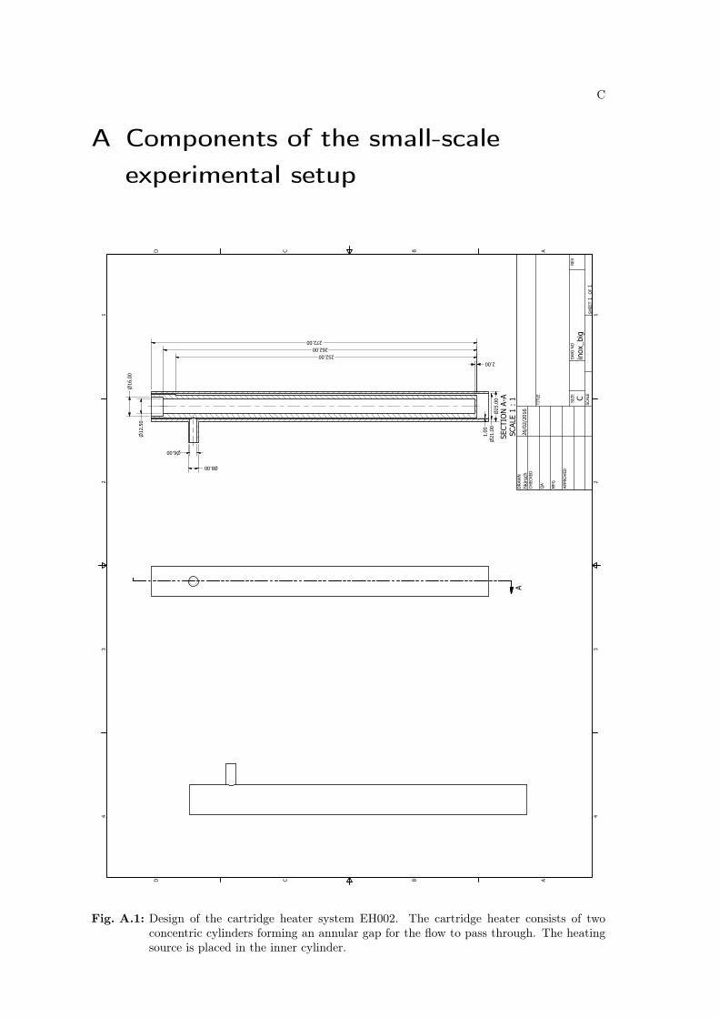
C
A Components of the small-scaleexperimental setup
SECTIO
N A-A
SCALE 1 : 1
A
1 1
2 2
3 3
4 4
AA
BB
CC
DD
SH
EET 1 O
F 1
DRAW
N
CH
ECKED
QA
MFG
APPRO
VED
hkirsch
26/02/2016
DW
G N
O
inox_big
TITLE
SIZE
C
SCALE
REV
1.00
6.00
8.00 Ø
12.50
16.00
21.00
25.00
Ø
2.00
252.00
262.00
272.00
Fig. A.1: Design of the cartridge heater system EH002. The cartridge heater consists of twoconcentric cylinders forming an annular gap for the flow to pass through. The heatingsource is placed in the inner cylinder.
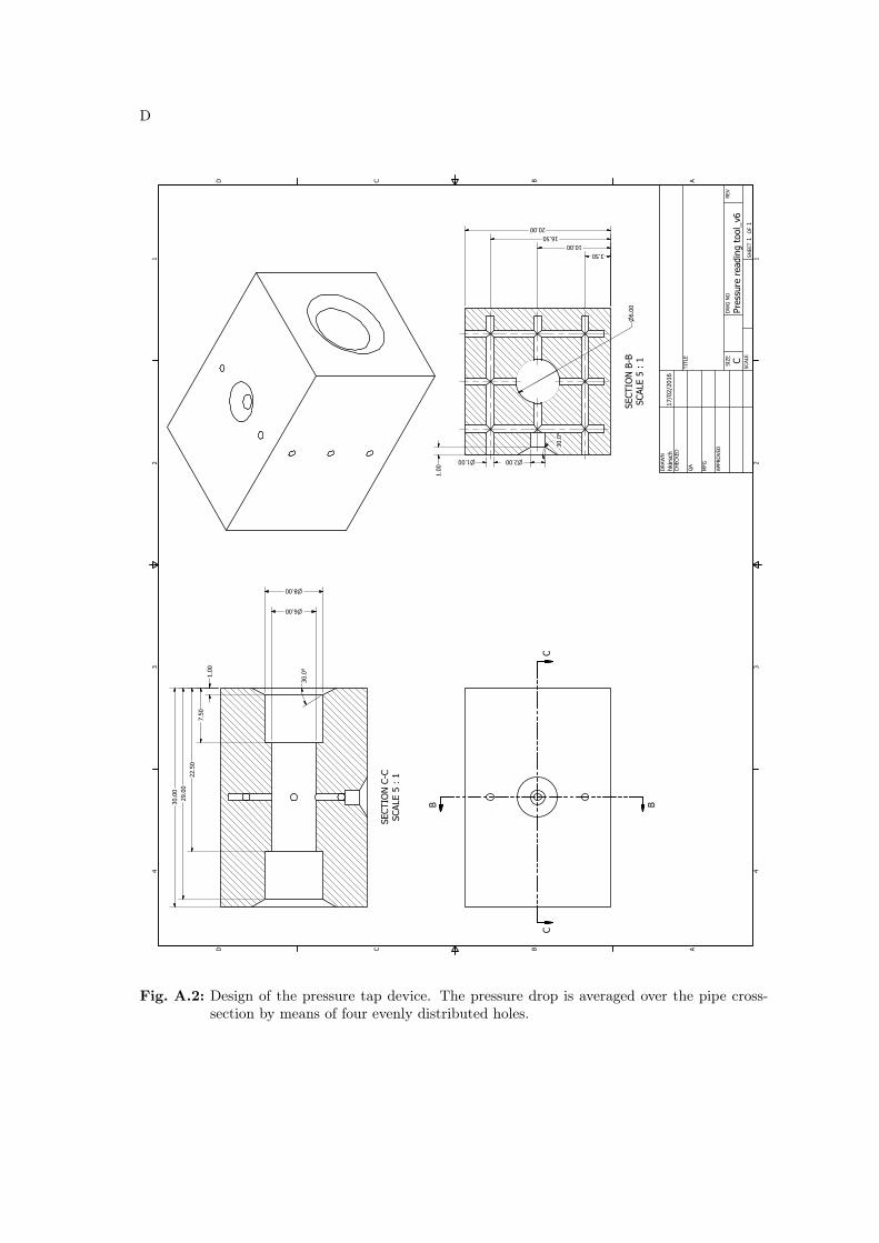
D
SECTIO
N B-B
SCALE 5 : 1
SECTIO
N C-C
SCALE 5 : 1
B B
CC
1 1
2 2
3 3
4 4
AA
BB
CC
DD
SH
EET 1 O
F 1
DRAW
N
CH
ECKED
QA
MFG
APPRO
VED
hkirsch
17/02/2016
DW
G N
O
Pressure reading tool_v6
TITLE
SIZE
C
SCALE
REV
8.00
6.00
30.0°
6.00
3.50
10.00
16.50
20.00
1.00 2.00
30.0°
1.00
1.00
7.50
22.50
29.00
30.00
Fig. A.2: Design of the pressure tap device. The pressure drop is averaged over the pipe cross-section by means of four evenly distributed holes.

B Matlab R© program
The Matlab R© program calculates the pressure drop of nitrogen two-phase flow at saturationpressures in the range of 2.6 bar to 2.9 bar. Variables in red have to be specified by theuser. Different void fraction and frictional pressure drop correlations (highlighted in blue)can be embedded into the program.
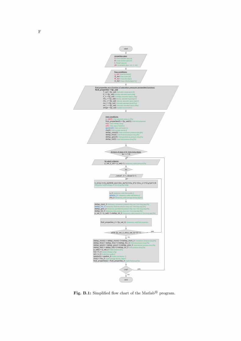
F
start
division of pipe in N 1mm-long steps:
for i = 1:N
fluid properties as a function of saturation pressure (embedded function):
fluid_properties = f(p_sat)
T_sat = f(p_sat) //saturation temperature [K]
h_l = f(p_sat)//enthalpy saturated liquid [J/kg]
h_v = f(p_sat) //enthalpy saturated vapour [J/kg]
rho_l = f(p_sat)//density saturated liquid [kg/m³]
rho_v = f(p_sat) //density saturated vapour [kg/m³]
mu_l = f(p_sat) //viscosity saturated liquid [Pas]
mu_v = f(p_sat) //viscosity saturated vapour [Pas]
simga = f(p_sat) //surface tension [N/m]
properties pipe:
d //inner diameter pipe [m]
A //cross section pipe [m²]
L //length pipe [m]
phi //orientation pipe (-π/2, 0, π/2)
end
i<N?
deltap_mom_it //temporary momentum pressure drop over 1mm-long step [Pa]
deltap_fric_it //temporary frictional pressure drop over 1mm-long step [Pa]
deltap_grav_it //temporary gravitational pressure drop over 1mm-long step [Pa]
deltap_tot_it //temporary total pressure drop over 1mm-long step [Pa]
p_sat_it = p_sat(i-1)-deltap_tot_it //temporary outlet pressure of 1mm-long step [Pa]
h_it=h(i-1)+Q_dot/N/M_dot-0.5m_dot^2(1/rho_it^2-1/rho_(i-1)^2)-g*phi*L/N//temporary outlet enthalpy of 1mm-long step [J/kg]
x_it //temporary outlet flow quality []
epsilon_it // temporary outlet void fraction []
rho_it //temporary outlet average density [kg/m³]
inlet conditions:
p_sat(0) //inlet saturation pressure [Pa]
fluid_properties(0) = f(p_sat(0)) //inlet fluid properties
h(0) //inlet enthalpy [J/kg]
x(0) //inlet vapour fraction []
epsilon(0) //inlet void fraction []
rho(0) //inlet average density []
deltap_mom(0) //inlet momentum pressure drop [Pa]
deltap_fric(0) //inlet frictional pressure drop [Pa]
deltap_grav(0) //inlet gravitational pressure drop [Pa]
deltap_tot(0) //inlet total pressure drop [Pa]
„values“_it = „values“(i-1)
fluid_properties_it = f(p_sat_it) //temporary outlet fluid properties
while (|p_sat_it_old-p_sat_it|>10^-7)
do
for abort criterion
p_sat_it_old = p_sat(i-1) //temporary outlet pressure [Pa]
deltap_mom(i) = deltap_mom(i-1)+deltap_mom_it //momentum pressure drop [Pa]
deltap_fric(i) = deltap_fric(i-1)+deltap_fric_it //frictional pressure drop [Pa]
deltap_grav(i) = deltap_grav(i-1)+deltap_grav_it //gravitational pressure drop [Pa]
deltap_tot(i) = deltap_tot(i-1)+deltap_tot_it //total pressure drop [Pa]
p_sat(i) = p_sat_it //outlet pressure [Pa]
h(i) = h_it //outlet enthalpy [J/kg]
x(i) = x_it //outlet flow quality []
epsilon(i) = epsilon_it //outlet void fraction []
rho(i) = rho_it //outlet average density [kg/m³]
fluid_properties(i) = fluid_properties_it //outlet fluid properties
flow conditions:
q_dot //heat flux [W/m²]
Q_dot //heat power [W]
M_dot //mass flow [kg/s]
m_dot //mass velocity [kg/(m²s)]
yes
no
yes
no
Fig. B.1: Simplified flow chart of the Matlab R© program.
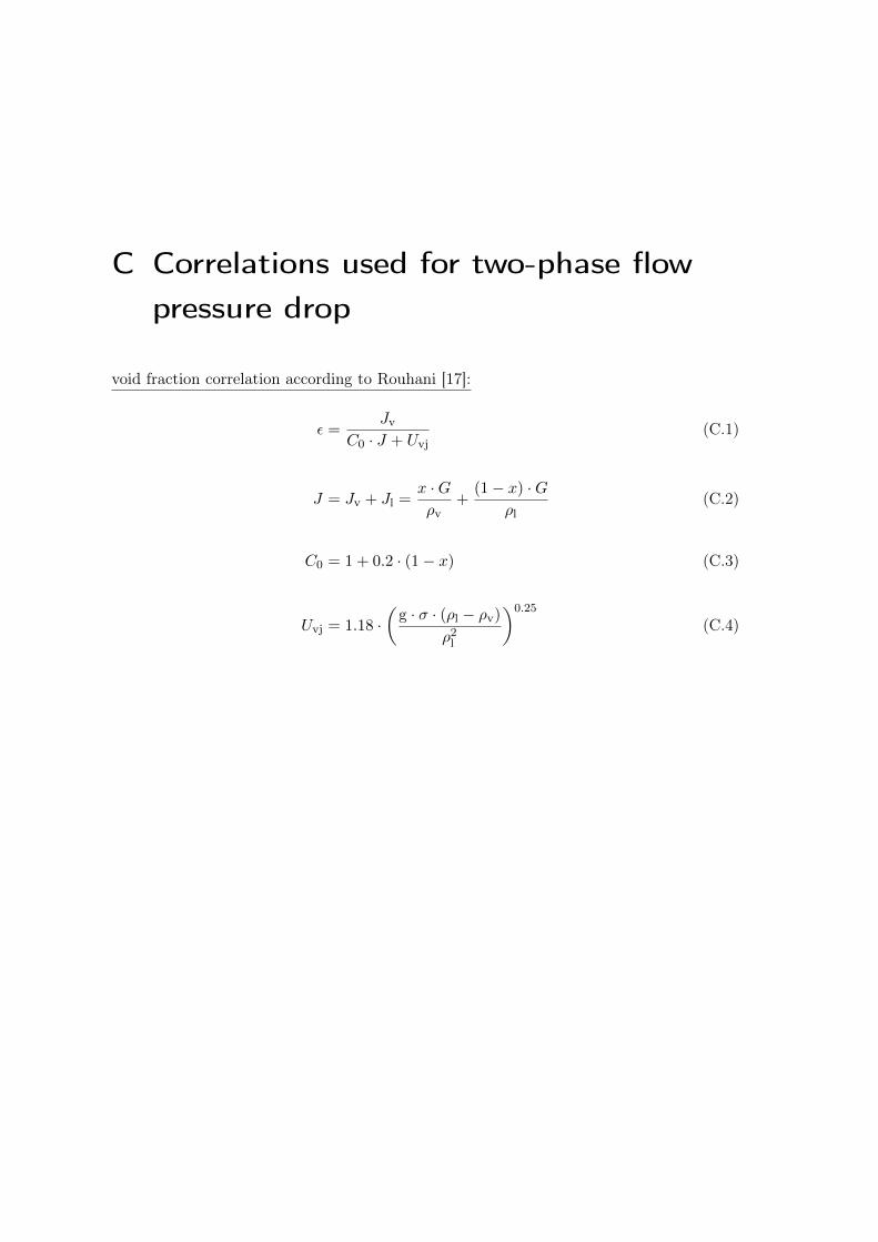
C Correlations used for two-phase flowpressure drop
void fraction correlation according to Rouhani [17]:
ε =Jv
C0 · J + Uvj(C.1)
J = Jv + Jl =x ·Gρv
+(1− x) ·G
ρl(C.2)
C0 = 1 + 0.2 · (1− x) (C.3)
Uvj = 1.18 ·(
g · σ · (ρl − ρv)
ρ2l
)0.25
(C.4)
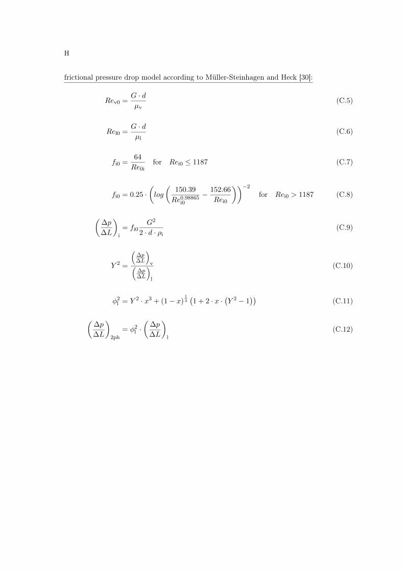
H
frictional pressure drop model according to Müller-Steinhagen and Heck [30]:
Rev0 =G · dµv
(C.5)
Rel0 =G · dµl
(C.6)
fi0 =64
Re0ifor Rei0 ≤ 1187 (C.7)
fi0 = 0.25 ·(log
(150.39
Re0.98865i0
− 152.66
Rei0
))−2
for Rei0 > 1187 (C.8)
(∆p
∆L
)i
= fi0G2
2 · d · ρi(C.9)
Y 2 =
(∆p∆L
)v(
∆p∆L
)l
(C.10)
φ2l = Y 2 · x3 + (1− x)
13(1 + 2 · x ·
(Y 2 − 1
))(C.11)
(∆p
∆L
)2ph
= φ2l ·(
∆p
∆L
)l
(C.12)