Embed Size (px)
Citation preview
econstor www.econstor.eu
Der Open-Access-Publikationsserver der ZBW – Leibniz-Informationszentrum WirtschaftThe Open Access Publication Server of the ZBW – Leibniz Information Centre for Economics
Standard-Nutzungsbedingungen:
Die Dokumente auf EconStor dürfen zu eigenen wissenschaftlichenZwecken und zum Privatgebrauch gespeichert und kopiert werden.
Sie dürfen die Dokumente nicht für öffentliche oder kommerzielleZwecke vervielfältigen, öffentlich ausstellen, öffentlich zugänglichmachen, vertreiben oder anderweitig nutzen.
Sofern die Verfasser die Dokumente unter Open-Content-Lizenzen(insbesondere CC-Lizenzen) zur Verfügung gestellt haben sollten,gelten abweichend von diesen Nutzungsbedingungen die in der dortgenannten Lizenz gewährten Nutzungsrechte.
Terms of use:
Documents in EconStor may be saved and copied for yourpersonal and scholarly purposes.
You are not to copy documents for public or commercialpurposes, to exhibit the documents publicly, to make thempublicly available on the internet, or to distribute or otherwiseuse the documents in public.
If the documents have been made available under an OpenContent Licence (especially Creative Commons Licences), youmay exercise further usage rights as specified in the indicatedlicence.
zbw Leibniz-Informationszentrum WirtschaftLeibniz Information Centre for Economics
Brunner, Johann K.; Pech, Susanne
Working Paper
Taxing Bequests and Consumption in the SteadyState
CESifo Working Paper, No. 4453
Provided in Cooperation with:Ifo Institute – Leibniz Institute for Economic Research at the University ofMunich
Suggested Citation: Brunner, Johann K.; Pech, Susanne (2013) : Taxing Bequests andConsumption in the Steady State, CESifo Working Paper, No. 4453
This Version is available at:http://hdl.handle.net/10419/89736
Taxing Bequests and Consumption in the Steady State
Johann K. Brunner Susanne Pech
CESIFO WORKING PAPER NO. 4453 CATEGORY 1: PUBLIC FINANCE
OCTOBER 2013
An electronic version of the paper may be downloaded • from the SSRN website: www.SSRN.com • from the RePEc website: www.RePEc.org
• from the CESifo website: Twww.CESifo-group.org/wp T
CESifo Working Paper No. 4453
Taxing Bequests and Consumption in the Steady State
Abstract We study the optimal tax system in a dynamic model where differences in wages induce differences in inheritances, and the transition from parent ability to child ability is described by a Markov chain. We characterize expected inheritances in the steady state and show that the Atkinson-Stiglitz result on the redundancy of indirect taxes does not hold in this framework. In particular, given an optimal income tax, a bequest tax as well as a consumption tax are potential instruments for additional redistribution. For the bequest tax the sign of the overall welfare effect depends on the reaction of bequests and on inequality aversion, while for the consumption tax the sign is always positive because the distorting effect is outweighed by the induced increase in wealth accumulation. A necessary condition for a positive welfare effect is the empirically validated relation that more able individuals on average have more able parents than less able individuals.
JEL-Code: H210, H240.
Keywords: optimal taxation, bequest tax, consumption tax.
Johann K. Brunner University of Linz
Department of Economics Altenberger Straße 69 Austria – 4040 Linz
Susanne Pech University of Linz
Department of Economics Altenberger Straße 69 Austria – 4040 Linz
[email protected] October 21, 2013
1 Introduction
In developed economies each year a substantial amount of wealth is transmitted from one
generation to the next (see Piketty 2011, Wol¤ 2002). Hence, inheritances represent an
important source of individual wealth, but their variation across individuals also creates
additional inequality in a society, on top of di¤erences in income. In this paper we study the
implications of this fact for the design of the tax system. In particular, we ask whether the
existence of inheritances requires speci�c tax instruments such as an estate tax to mitigate
inequality. As is well-know, inheritance taxation is one of the most controversial issues in
tax policy.
To provide an answer to this question we formulate a dynamic optimal-taxation model
of an economy with individuals di¤ering in labor productivity and leaving bequests to their
descendants. We ask how a shift from labor-income taxation to bequest or consumption
taxation a¤ects welfare in the steady state of this economy. The starting point is the
well-known result by Atkinson and Stiglitz (1976) derived in a model without bequests:
if labor income is taxed optimally then any other - indirect - tax is redundant, given
weak separability of preferences in consumption and labor.1 As a consequence, if leaving
bequests is just seen as one form of consumption, there is no role for a tax on estates;2
neither is any kind of consumption or capital taxation useful. In particular, an estate tax
does not allow more redistribution than what is possible through an income tax alone.3
The situation changes if one takes into account that, as the very consequence of wealth
transmission from parents to children, individuals of some generation di¤er not only in
abilities but also in inherited wealth. Brunner and Pech (2012ab) have shown that with
exogenously given inherited wealth a tax on wealth transfers indeed has a redistributive
e¤ect, given that more productive individuals receive more inheritances.4
1This holds in case of an optimal nonlinear income tax. If it is restricted to be linear the condition thatpreferences over consumption are homothetic is needed (see Deaton 1979).
2Unless bequests are a complement to leisure, see e.g., Gale and Slemrod (2001), Kaplow (2001).3On the contrary, one can also take the view that even a subsidy for bequests increases welfare. The
reason is the positive external e¤ect associated with bequests, because in addition to the value theyprovide for the donor, they also contribute to utility of the recipient (see Farhi and Werning (2010), amongothers). Recently, Kopczuk (2013a) has presented a formula for the optimal nonlinear tax on bequestswhich accounts for the positive externality as well as for the negative income e¤ect of received inheritanceson labor supply of children.
4 In a related approach, Boadway et al. (2000) and Cremer et al. (2001, 2003) show that indirect
1
In contrast, in the present paper we analyze the welfare consequences of taxes in the
steady-state equilibrium of an economy, when inheritances are completely endogenous.
More precisely, we formulate a dynamic model where in each period a new generation
consisting of n di¤erent ability groups of individuals exists. Each individual is the parent
of one child, who again belongs to one of the n groups in the next generation. The
transition probabilities from parent ability to child ability are constant over time; the
stochastic process can be described by a Markov chain and we consider the steady-state
distribution of abilities.
Each individual uses her labor income and received inheritances for own consumption
and for leaving bequests to her single child of the next generation. Depending on the
transition probabilities, the budget share devoted to bequests in each group determines
the distribution of inheritances over groups in the next generation. The same transition
occurs in later periods and eventually leads to a steady-state distribution of inheritances,
within and across ability groups. This distribution is rather diverse, as it depends on all
bequest decisions of all prior generations. Still, under the assumption of a¢ ne-linear Engel
curves for consumption and bequests in each period, we are able to characterize expected
inheritances of each ability group in the steady-state.
As a result we arrive at a Mirrlees-type model with di¤ering labor productivities, ex-
tended by the existence of endogenously determined inheritances. We then apply this
model to study the optimal design of a tax system. First we analyze the optimal linear in-
come tax, determined by maximization of expected social welfare of a generation. It turns
out that in the extended model the redistributive e¤ect of this tax is more pronounced,
because it refers not only to labor income as such, but also indirectly to steady-state in-
heritances �nanced by labor income. On the other hand, the distortion of labor supply
causes an indirect negative e¤ect on inheritances. Altogether, the desirability of a positive
marginal tax rate is guaranteed if the labor supply elasticity is not too large.5
Next, we address the main question, namely whether the introduction of indirect taxes
taxes as well as a tax on capital income make sense if individuals di¤er in inherited wealth. They assume,however, that bequests and inheritances are unobservable and, thus, cannot be taxed. In Saez (2002)exogenous di¤erences in the tastes for consumption goods make indirect taxes useful.
5This is in contrast to the static, one-period model where the optimal marginal tax rate is unambiguouslypositive (see e.g., Hellwig 1986, Brunner 1989).
2
on bequests or consumption increases steady-state social welfare, given an optimal linear
income tax. The answer to this question is unclear a priori, because on the one hand we
know for the bequest tax that it is desirable if individuals di¤er in a second exogenously
given characteristic, namely inherited wealth (in addition to labor productivities). On the
other hand, however, in the steady-state the di¤erences in (expected) inheritances are in
fact the consequence of the di¤erences in labor productivities. Therefore, as the latter
represent the only (exogenous) source of heterogeneity, one might suppose that again the
Atkinson-Stiglitz result applies and no other (indirect) tax than the optimal labor income
tax is desirable.
Our analysis shows that this conjecture is wrong. We �rst �nd a speci�c redistributive
role of the bequest tax in the steady-state of the economy if the condition that more
productive individuals also receive higher expected inheritances is ful�lled. On the other
hand, the tax distorts the bequest decision and induces, thus, lower accumulated wealth
in the steady state. The overall e¤ect is positive in case that the substitution elasticity
between bequests and consumption is small or that the degree of inequality aversion in
the social welfare function is high.
Further, we �nd for a consumption tax, introduced in addition to an optimally chosen
tax on labor income, that in our model it has a redistributive potential similar to the
bequest tax. A closer analysis shows that both taxes, though being targeted on some form
of spending of the individuals�budgets (for bequests versus own consumption), in fact are
instruments for an equalization of received (inherited) wealth. The di¤erence is, however,
that the distortion caused by the consumption tax works in favor of bequests and induces,
thus, a higher accumulation of wealth. For small tax rates, this accumulation e¤ect is
large enough to outweigh the deadweight loss so that the overall e¤ect of a consumption
tax is unambiguously positive. This result can be seen as a justi�cation of a speci�c tax on
consumption which in fact exists in many countries, like the VAT in the European Union.
It should be stressed that in standard optimal-taxation models such a tax has no
particular role: if the individuals�budget consists only of labor income which is spent for
the consumption of di¤erent commodities, a uniform tax on the latter is equivalent to an
income tax. In our model the analogous instrument is a uniform tax on bequests and
3
consumption which we call an expenditure tax. We show that such a tax unambiguously
increases social welfare e¤ect, because it combines the redistributive e¤ect of both separate
taxes and causes no distortion.
For these results again the condition that in the steady-state more able individuals
receive higher expected inheritances is crucial. This condition actually requires that a more
able individual on average has more able parents than a less able individual. That this
conforms to reality can be concluded from a number of empirical studies on the correlation
between parent and child income. The pioneering work by Solon (1992) and Zimmerman
(1992) found an intergenerational correlation in the long-run income (between fathers and
sons) of around 0.4 for the United States (suggesting less social mobility than previously
believed). By now, there is a large set of estimates for a range of di¤erent countries (for
a recent overview see Black and Devereux 2011 and Leigh 2007). Although these studies
used di¤erent estimation methods, variable de�nitions and sample selections (limiting their
comparability), all of them estimated a positive intergenerational correlation in earnings,
ranging from 0.1 up 0.4, which corroborates the above condition.6
Our study establishes a role for indirect taxation as an instrument for increasing equal-
ity of opportunity. In a related work Piketty and Saez (2013) derive a formula for the op-
timal bequest tax rate in terms of estimable parameters such as the elasticity of bequests
with respect to the tax. Taking the amount of government transfers as given, this formula
states to which extent they should be �nanced by a tax on bequests as opposed to a tax
on labor income, depending on the parameter constellation. In contrast, our focus is on
whether a welfare gain by additional redistribution through indirect taxes is possible, given
an optimal linear income tax. In particular, we also characterize the speci�c e¤ects of a
consumption or expenditure tax arising from di¤erences in inheritances across individuals.
In the following Section we present the basic model of individual decisions on labor
supply, consumption and bequests. Section 3 provides an analysis of the dynamics of
wealth transmission over generations, whose steady state is studied in Section 4. In Section
6 In particular, these studies suggest that the correlation in the Nordic countries (Sweden, Finland,Denmark, Norway), Canada and Australia is about 0.1 � 0.2 and thus lower than in the U.S. and U.K.Interestingly, Jäntti et al. (2006) �nd that the greatest cross-country di¤erences arise at the tails ofdistribution. Moreover, these studies estimate higher correlations between son and father than betweendaughter and farther, while the pattern across countries is similar.
4
5 the optimal tax on labor income is characterized, and the results on the desirability of
additional taxes on bequests and consumption, respectively, are derived. Section 6 provides
an extensive discussion of these results.
2 The Model
In each period t a population of mass one exists. It is split into n groups with di¤er-
ent abilities w1 < w2 < :::: < wn, whose shares are f1; :::; fn. That is, f1; :::; fn are
the probabilities of an individual to belong to the respective ability group. Individuals
of a generation live for one period; they have common preferences over consumption ci,
labor time li, and leaving bequests bi. Preferences are described by the utility function
u(ci; bi; li) = '(ci; bi)� g(li), where ' is a concave function, increasing in both arguments,
and g is strictly concave and increasing. This formulation indicates that we assume be-
quests to be motivated by joy-of-giving. Pre-tax labor income is wili and the individual
receives inheritances ei; i = 1; :::; n.
There exists a linear tax on labor income, given by ��+ �wili with �� as a uniform
negative tax and � as the marginal tax rate on gross labor income. Moreover, the tax
system consists of a proportional tax � b on bequests and of a proportional tax � c on
consumption. For given taxes the maximization problem of an individual i is
max'(ci; bi)� g(li); (1)
s.t. (1 + � c)ci + (1 + � b)bi � ei + �+ (1� �)wili; (2)
ci; bi; li � 0: (3)
The �rst-order conditions for an interior solution with � as the Lagrangian variable asso-
ciated with (2) read as@'
@ci� �(1 + � c) = 0; (4)
@'
@bi� �(1 + � b) = 0; (5)
5
�g0(li) + �(1� �)wi = 0: (6)
From these we obtain demand functions for ci and bi. We assume that demand can be
described by linear Engel curves which need not pass through the origin. That is, ci and
bi can be written as shares (1� )=(1+ � c) and =(1+ � b), with 2 (0; 1), of the available
budget, given a constant ca representing minimum consumption:
ci = c(ei + xi � (1 + � c)ca) + ca; (7)
bi = b(ei + xi � (1 + � c)ca): (8)
Here xi denotes net income of the household, xi � � + (1 � �)wili, and b � =(1 + � b)
describes the share of bequests in the "real" budget after deducting minimum consumption,
while c � (1 � )=(1 + � c) describes the corresponding share of consumption above
minimum consumption. We generally assume that the expenditures for ca are not larger
than net income, that is, xi � ca(1 + � c) > 0.
Such a type of demand functions, as described by (7) and (8), arises if ' can be
written as a function e'(ci� ca; bi), homogeneous in ci� ca and bi. In addition, we assumethat e' is homogeneous of degree 1. Note that in general itself depends on � b and
� c, such as in case of a properly adjusted CES utility function with the functional forme'(ci � ca; bi) = ((1 � �)1��(ci � ca)� + �1��b�i )1� where the parameters � and (1 � �),
respectively, express the weights on bi and ci�ca, while � determines the constant elasticity
of substitution 1=(1� �):7
Indirect utility of an individual i is given by evaluating '(ci; bi) � g(li) at the values
(7) and (8) and with li determined by (6). Linear homogeneity of e' implies that e'( c(ei+xi � (1 + � c)ca); b(ei + xi � (1 + � c)ca) = �(ei + xi � (1 + � c)ca), where � = e'( c; b)is the marginal utility of income which is independent of wi; ei and xi but depends on � c
and � b. Hence, indirect utility Vi is given by
Vi(ei;�; �; � c; � b) = �(ei + xi � ca(1 + � c))� g(li) (9)
7Only in case of a Stone-Geary utility function (ci � ca)1��b�i (� converges to zero), is the constantweight � of bequests.
6
where li is determined by (6) as li = (g0)�1(�(1� �)wi), depending on the after-tax wage
rate (1 � �)wi and on the marginal utility of income �. Note that from (6) the relation
x1 < x2 < ::: < xn follows, because � is independent of wi.
3 Dynamics of wealth transmission and abilities
Having speci�ed the model of the economy in any given period, including the individual
decision to bequeath part of the available budget to the descendants, we now turn to the
dynamics. We consider the transmission of wealth in detail and study the distribution
of inheritances in the steady-state of this process. We assume that abilities w1 < w2 <
:::: < wn remain constant over time (that is, over generations). Each individual has a
single descendant to whom she leaves all her bequests. There is a constant transition
probability pij that an individual with ability wi has a descendant with ability wj ; wherePnj=1 pij = 1 for i = 1; :::; n: With constant transition probabilities the dynamics of the
shares of the ability groups over time represents a Markov chain. We assume the Markov
chain to be ergodic and to converge to a steady-state distribution � = (�1; :::; �n): � is
unique and independent of the initial distribution f � (f1; :::; fn); it is determined by
the equation � = �P together with the normalizationPni=1 �i = 1, where P is the n� n
transition matrix with entries pij . As is well-known, � can be found by considering the limit
W � limt!1 P t: All n rows ofW are identical and equal to �. We assume in the following
that the distribution of abilities is already in the steady-state, that is fi = �i; i = 1; :::; n.
Thus, f has the property
f = fP: (10)
Next we study the transmission of bequests. Tax parameters �; � and � b, � c are assumed
to remain constant over time, therefore labor supply and net income of each type is also
constant over time. Let bjt be the bequests left by an individual with ability wj in some
period t. We study the di¤usion of these bequests to the individuals of the next generation
t+ 1.
Let ei;t+1 denote inheritances received in period t+1 by an individual in ability group
i out of bequests of the preceding period. Clearly, each ei;t+1 has possible realizations
7
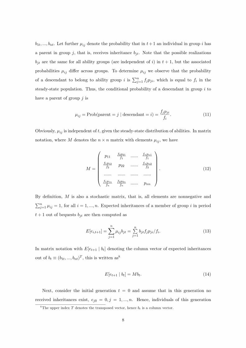
b1t; :::; bnt. Let further �ij denote the probability that in t+1 an individual in group i has
a parent in group j, that is, receives inheritance bjt. Note that the possible realizations
bjt are the same for all ability groups (are independent of i) in t + 1, but the associated
probabilities �ij di¤er across groups. To determine �ij we observe that the probability
of a descendant to belong to ability group i isPnj=1 fjpji, which is equal to fi in the
steady-state population. Thus, the conditional probability of a descendant in group i to
have a parent of group j is
�ij = Prob(parent = j j descendant = i) =fjpjifi
: (11)
Obviously, �ij is independent of t, given the steady-state distribution of abilities. In matrix
notation, where M denotes the n� n matrix with elements �ij , we have
M =
0BBBBBBB@
p11f2p21f1
:::::: fnpn1f1
f1p12f2
p22 :::::: fnpn2f2
:::::: :::::: :::::: ::::::
f1p1nfn
f2p2nfn
:::::: pnn
1CCCCCCCA: (12)
By de�nition, M is also a stochastic matrix, that is, all elements are nonnegative andPnj=1 �ij = 1, for all i = 1; :::; n. Expected inheritances of a member of group i in period
t+ 1 out of bequests bjt are then computed as
E[ei;t+1] =nXj=1
�ijbjt =nPj=1
bjtfjpji=fi: (13)
In matrix notation with E[et+1 j bt] denoting the column vector of expected inheritances
out of bt � (b1t; :::; bnt)T ; this is written as8
E[et+1 j bt] =Mbt: (14)
Next, consider the initial generation t = 0 and assume that in this generation no
received inheritances exist, ej0 = 0; j = 1; :::; n. Hence, individuals of this generation8The upper index T denotes the transposed vector, hence bt is a column vector.
8
leave bequests out of labor income only, bj0 = b(xj0 � ca(1 + � c)), and these values are
the possible realizations of inheritances ei1 received by an individual i in generation 1.9
Furthermore, with homothetic preferences, bequests left by an individual i in generation
1 can be separated into those out of received inheritances and those out of own labor
income, that is, bi1 = bei1 + b(xi1 � ca(1 + � c)). As a consequence, we get bi1 =
2b(xj0� ca(1+ � c)) + b(xi1� ca(1+ � c)), for some j 2 f1; :::; ng. By the same reasoning,
bequests left by an individual k in generation 2 can be expressed as bk2 = 3b(xj0� ca(1+
� c)) + 2b(xi1 � ca(1 + � c)) + b(xk2 � ca(1 + � c)), for some i; j 2 f1; :::; ng, which are the
possible realizations of inheritances em3 for any individual m (independent of the type) in
generation 3.
Generalizing this idea we �nd that in any generation t received inheritances of an
individual r 2 f1; :::; ng can assume one of the values
ert =t�1Xs=0
t�sb (xjss � ca(1 + � c)); js 2 f1; :::; ng, (15)
which again are the same for any r. What is inherited by some individual in t only
depends on the ability group of the individual who originally leaves bequests out of own
labor income; but is independent of the ability types of individuals further involved in
the transition process by just transmitting a share b of received inheritances to the next
generation. Obviously, because of this decline by the factor b, total inheritances in
each generation are dominated by bequests originating from labor income of more recent
generations.
One observes that the number of possible realizations increases by the factor n in
each generation, when received inheritances are combined with n values of labor income.
Fortunately, we need not describe the distribution in detail but con�ne our analysis to
the evolution of expectations. Clearly, the above insights also remain true in the long
run, for t going to in�nity. In particular, given our assumption of constant abilities, the
values xjs � ca(1 + � c) in (15) are obviously bounded by xn � ca(1 + � c) for all s,10 thus9For the moment, to make the time structure more transparent, we add a time index to net income
(which in fact is constant over time for each type, given constant tax rates).10From now we drop the time index to net income again.
9
for t!1 inheritances are not larger than (xn� ca(1+ � c)) b=(1� b). This implies that
all realizations of inheritances are �nite, then also expected inheritances of each group are
�nite for all t going to in�nity.
For a characterization of expected inheritances we return to formula (14) which de-
scribes the relation between bequests and inheritances of succeeding generations. We know
that in generation t bequests result as bjt = b(ejt + xj � ca(1 + � c)), with received inher-
itances ejt being a random variable, j = 1; :::; n. In vector notation, with column vectors
et = (e1t; :::; ent)T ; x = (x1; :::; xn)
T and cva = (ca; :::; ca)T , (14) reads as
E[et+1 j et] = bM(et + x� cva(1 + � c)) (16)
and computing the expectation over all possible realizations of et gives11
E[et+1] = bM(E[et] + x� cva(1 + � c)). (17)
That is, the matrix M governs the evolution of expected values over time.
4 The steady-state
We have assumed from the beginning that the population is constant and the distribution
of abilities is in the steady-state, that is, the shares fi of all groups remain constant over
time. Note that because of our assumption of a population of mass one, split into n ability
groups, expected inheritances are equal to realized inheritances; there is no aggregate
uncertainty. The overall steady-state of this economy is de�ned by the condition that
expected inheritances of each ability group also remain constant over time, that is
E[e] = bM(E[e] + x� cva(1 + � c)) (18)
11Formally, let H denote the index set of all possible realizations eth of the vector et, with associ-ated probabiliies �th; h 2 H (thus �t1 + �t2 + ::: = 1). Then E[et+1] =
Ph2H �thE[et+1 j eth] =P
h2H �th bM(eth + x� (1 + � c)cvs) = bM(E[et] + x� (1 + � c)cvs).
10
or
E[e] = A(x� cva(1 + � c)); (19)
with A � b(I � bM)�1M and I denoting the unit matrix. In view of the formula for a
geometric series, (I � bM)�1 =P1t=0( bM)
t, equation (19) can be written as
E[e] =1Xt=1
tbMt(x� cva(1 + � c)); (20)
which suits well to our earlier result (see (15)) that inheritances in some period consist of
bequests out of labor income in all past periods.
Before we turn to the optimal tax problem we discuss a condition on M which will
turn out to be important in the next section:
De�nition 1 A n � n matrix Z ful�lls condition (C), if for any column vector y 2 Rn
with increasing components, y1 < y2 < ::: < yn, the column vector Zy also has increasing
components.
For an interpretation of this condition in our framework let some vector x of steady-
state net incomes of the n groups in the descendant generation be given and consider
the parents of each descendant group. By de�nition, the column vector Mx describes
mean parent net incomes for each group and condition (C) states that, given increasing
incomes in each generation, mean parent income is increasing as well. As mentioned in the
introduction, there is substantial empirical evidence that parent and descendant income is
positively correlated, therefore it seems indeed very plausible that condition (C) is ful�lled
in reality. One observes immediately from (20) that whether M ful�lls these condition is
also essential for the question of how incomes and inheritances are related.
Lemma 1 The matrix A has nonnegative elements and the components of each of its row
vectors sum up to b=(1 � b). Moreover, if M has property (C), then also A has this
property; that is expected inheritances are increasing with abilities.
Proof. We know that A can be written asP1t=1( bM)
t. Elementary properties of matrix
multiplication show that in each term of the in�nite series the row vectors have components
11
adding up to tb (remember that components of the rows of M add up to 1 and the same
is true for M t, for any t), which gives the sumP1t=1
tb = b=(1� b). Multiplying by y,
each term in the in�nite series consists of the product tb M �M �M::::My (whereM occurs
t-times). Clearly, if My has increasing components, then M ty has increasing components
as well, and this remains true after multiplication with tb and summing up the terms.
A su¢ cient condition on M to ful�ll (C) is that the components of the column vectors
of M are increasing above and decreasing below the diagonal, with the diagonal element
being the largest:
Lemma 2 Let the �ij, the elements of M , have the following properties:
�ii > �ji for any i; j = 1; ::; n; i 6= j (21)
�ij � �i+1;j for j < i � n� 1; (22)
�ij � �i+1;j for 1 � i � j � 2: (23)
Then M ful�lls condition (C).
Proof. Assume that M has the properties (21) - (23). Consider two subsequent rows Mi
andMi+1 ofM . Construct fMi fromMi by reducing the �rst i components ofMi to those of
Mi+1 and increasing the component �i;i+1 appropriately so that the sum of all components
remains 1: For any vector y with increasing components yi this gives fMiy > Miy. If fMi
is equal to Mi+1; we are ready. Otherwise, in a second step, if some of the remaining
components i+ 2; :::; n of fMi (namely, of Mi) are smaller than the corresponding ones of
Mi+1, increase the former to the latter and decrease the i+1-component of fMi so that the
sum of all components remains 1: The resulting vector is Mi+1 and because of increasing
yi we altogether have Mi+1y � fMiy > Miy:
In fact, the property (C) is a condition on the transition matrix P , from which M is
derived (see 12). A general condition on P which implies (C) for M is not easily found.
Instead, we present two special cases of P such that M is equal to P: Then, clearly, if P
ful�lls (21) - (23), thenM ful�lls condition (C). Intuitively, the two cases are when (i) only
12
switches to neighboring ability groups are possible or when (ii) switches to other ability
groups are equally likely:
Lemma 3 Let P have one of the two properties:
(i) pij = 0 for j i� j j� 2
(ii) pij = di for j 6= i:
Then the probability matrix M is equal to the transition matrix P .
Proof. See Appendix.
Finally we note for later use that M has the same property as P :
Lemma 4 Let f be the steady-state distribution of abilities and the stochastic matrix M
de�ned as in (12). Then
f = fM: (24)
Proof. One observes immediately that fM = (f1(p11 + p12 + :::+ p1n); :::; fn(p11 + p12 +
:::+ p1n)) = f .
5 Optimal Taxes
Formula (19) characterizes steady-state inheritances in terms of labor supply lj ; j = 1; :::; n
and the share b of bequests which, in turn, depend on the tax parameters �; �; � b; � c,
�xed by the government. In this section we study how the government should choose
the tax parameters in order to maximize social welfare in the steady-state. In particular,
we are interested in the question of whether taxes on bequests or consumption (or on
both) are desirable instruments. It was already mentioned that, given an optimal tax
on labor income, both are redundant in a static one-period context of the model when
individuals receive no (or identical) inheritances, as a consequence of the Atkinson-Stiglitz
result (note that we have assumed weakly separable preferences). However, previous
work (Brunner and Pech 2012ab) has shown that this result does not apply in a model
with (exogenously given) di¤ering inheritances, which represent a second characteristic of
13
individuals in addition to di¤ering abilities.12 Now, in the model of this paper, inheritances
in the steady-state are not exogenous, but are ultimately determined by labor income of the
di¤erent groups. It is therefore a priori unclear whether taxes on bequests or consumption
represent desirable additional instruments or are redundant as in the Atkinson-Stiglitz
case.
In order to set up the maximization problem of the government we note �rst an im-
plication of linear homogeneity of e'(ci � ca; bi): expected utility Ph2H �ihe'( c(eh + xi �ca(1 + � c)); b(eh + xi � ca(1 + � c))), where eh denotes all possible realizations of e with
associated probabilities �ih, is equal to utility from expected inheritances e'( c(E[ei]+xi�ca(1+ � c)); b(E[ei]+xi� ca(1+ � c))).13 This allows us to formulate the problem of max-
imizing steady-state social welfare in the following way: let � > 0 denote the parameter
of inequality aversion and remember that '(ci; bi) = e'(ci � ca; bi), then the task is tomax
nPi=1
fi1� � ['( c(E[ei] + xi � ca(1 + � c)) + ca; b(E[ei] + xi � ca(1 + � c)))� g(li)]
1��;
(25)
s.t. �nPi=1fiwili � �+ � b
nPi=1fi b(E[ei] + xi � ca(1 + � c))
+ � cnPi=1fi( c(E[ei] + xi � ca(1 + � c)) + ca) � 0; (26)
E[ei] = Ai(x� cva(1 + � c)); (27)
where Ai denotes the i-th row vector of the matrix A = b(I � bM)�1M and x is the
column vector of net incomes with components xi = �+(1��)wili. Remember that Vi is
indirect utility (9) and � = @Vi=@xi is the marginal utility of income, independent of wi.
We note �rst
Lemma 5 If M has property (C) then V1 < V2 < � � � < Vn and V ��1 > V ��2 > � � � > V ��n :
Proof. With no (or identical) inheritances indirect utility Vi obviously rises with i because
of a higher net wage. Moreover, we know from Lemma (1) that, given property (C),
12To be precise, this result was shown for an optimal nonlinear tax on labor income. It is, however,straightforward to extend the result to the case of an optimal linar tax, given linear homogeneity of e'.13Remember that the realizations of e are the same for each ability group, but the associated probabilities
di¤er.
14
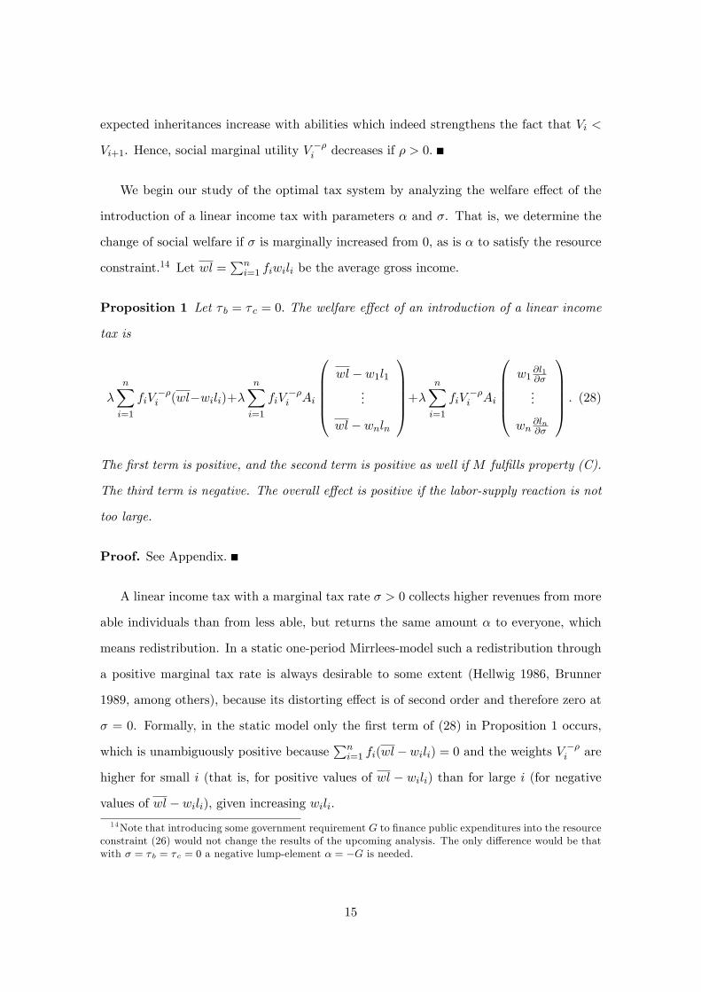
expected inheritances increase with abilities which indeed strengthens the fact that Vi <
Vi+1. Hence, social marginal utility V��i decreases if � > 0.
We begin our study of the optimal tax system by analyzing the welfare e¤ect of the
introduction of a linear income tax with parameters � and �. That is, we determine the
change of social welfare if � is marginally increased from 0, as is � to satisfy the resource
constraint.14 Let wl =Pni=1 fiwili be the average gross income.
Proposition 1 Let � b = � c = 0: The welfare e¤ect of an introduction of a linear income
tax is
�
nXi=1
fiV��i (wl�wili)+�
nXi=1
fiV��i Ai
0BBBB@wl � w1l1
...
wl � wnln
1CCCCA+�nXi=1
fiV��i Ai
0BBBB@w1
@l1@�
...
wn@ln@�
1CCCCA : (28)
The �rst term is positive, and the second term is positive as well if M ful�lls property (C).
The third term is negative. The overall e¤ect is positive if the labor-supply reaction is not
too large.
Proof. See Appendix.
A linear income tax with a marginal tax rate � > 0 collects higher revenues from more
able individuals than from less able, but returns the same amount � to everyone, which
means redistribution. In a static one-period Mirrlees-model such a redistribution through
a positive marginal tax rate is always desirable to some extent (Hellwig 1986, Brunner
1989, among others), because its distorting e¤ect is of second order and therefore zero at
� = 0. Formally, in the static model only the �rst term of (28) in Proposition 1 occurs,
which is unambiguously positive becausePni=1 fi(wl�wili) = 0 and the weights V
��i are
higher for small i (that is, for positive values of wl � wili) than for large i (for negative
values of wl � wili), given increasing wili.14Note that introducing some government requirement G to �nance public expenditures into the resource
constraint (26) would not change the results of the upcoming analysis. The only di¤erence would be thatwith � = � b = � c = 0 a negative lump-element � = �G is needed.
15
In our steady-state model, redistribution via the introduction of a linear tax on labor
income also a¤ects the amount of bequests left by each ability type, and the long-run
consequences on inheritances can be seen from the remaining terms of (28) in Proposition
1. If M ful�lls condition (C) then expected inheritances in the steady state (described by
Ai times the vector (x � cva) where xi = wili at � = � = 0) increase with abilities and
the second term shows that the introduction of the linear income tax - by redistributing
income - also makes the distribution of inheritances more equal.
As to the third term, note that in the static model without inheritances the welfare
loss caused by the introduction of the income tax (at � = 0), via its negative impact on
labor supply and income, is just compensated by the welfare gain through the associated
increase in leisure (the deadweight loss is zero). In the steady-state model with inheritances
an additional, indirect welfare loss, visible in the third - negative - term of (28), occurs
because the reduction of labor supply and income transforms into lower long-run bequests.
The overall welfare e¤ect of introducing a linear income tax is therefore positive if the
labor supply elasticity is small. Moreover, a positive overall e¤ect is the more likely, the
larger the �rst two terms in (28), that is, the larger the spread of individual incomes and
the degree of inequality aversion.
In the following we take as given that a positive marginal tax rate � is optimal, which
means that some redistribution of income is desirable. Obviously, with � > 0 the distorting
e¤ect on labor supply of the marginal tax rate becomes increasingly important, and � < 1
must hold in the optimum, otherwise labor supply would be zero, as follows from (6) with
g0(li) > 0. We now study the welfare e¤ects of taxes on bequests and on consumption and
ask whether their introduction makes sense as a supplement to an optimally chosen labor
income tax.
Let in the following e �Pni=1 fiE[ei] denote average inheritances received by a gen-
eration, and ev = (e; :::; e)T denote the corresponding column vector. Moreover, for any
matrix Z and tax parameter � we use the notation that [@Z=@�]i is row i of the matrix
derived from Z by di¤erentiating each component with respect to �. With S(� b; � c) de-
noting the optimal value function of the maximization problem (25) - (27), we �nd for the
bequest tax:
16
Proposition 2 Let � c = 0: The welfare e¤ect of an introduction of a tax � b on bequests,
given that the linear income tax is chosen optimally, is
@S
@� b
�����b=0
= �nXi=1
fiV��i (e� E[ei])
+�nXi=1
fiV��i
�@A
@� b
�i
(x� cva) + �nXi=1
fiV��i Ai(�e
v + x� cva): (29)
The �rst term is positive, given that M ful�lls property (C); the second term is negative,
and the third term is positive.
Given that M ful�lls property (C), the overall e¤ect on social welfare is positive (i) if the
elasticity of substitution between bequests and consumption is small, or (ii) if inequality
aversion is large and expected inheritances of the lowest-income group are small.
Proof. See Appendix.
Intuitively, the introduction of the bequest tax causes two separate e¤ects: the welfare
e¤ect for given inheritances (that is, holding inheritances �xed), which is the term in
the �rst line of the above formula, and the welfare e¤ect due to changes in steady-state
inheritances, which is described by the second line. The �rst e¤ect shows the main role
of the bequest tax: it allows additional redistribution of E[ei]; which is that particular
part of (expected) bequests �nanced out of (expected) received inheritances. If these are
increasing with i (M and hence A ful�ll condition (C), that is, more able individuals
receive larger inheritances), then the term in the �rst line of (29) is positive, because
the weights V ��i are decreasing. The point is that the bequest tax is an instrument for
equalization of received inheritances; it redistributes the latter indirectly via the share
used for bequests. (Clearly, the bequest tax is also imposed on the other part of bequests,
xi), which is �nanced out of net labor income. But for these - as the Atkinson-Stiglitz
result tells us - no further redistribution is possible in addition to that performed by
the optimal income tax.) The �rst term also occurs in the static model with exogenous
inheritances (Brunner and Pech 2012b).
The second e¤ect (second line of (29)) consists of two terms. The �rst (which is
negative) describes how the introduction of � b a¤ects the accumulation process as it reduces
17
the share b of income devoted to bequests. Note from the de�nition of Ai that it is indeed
only through the change of b that � b in�uences Ai. The last term (which is positive) in
(29) occurs because steady-state inheritances increase as a consequence of the fact that
the revenues from the bequest tax are redistributed via a lower marginal income tax �
and a larger lump-sum element �.
In order to gain further insights, we determine the e¤ect of � b on Ai (see the Appendix)
which allows us to rewrite the second line of (29) as
�nXi=1
fiV��i (Ai�e
v � Bi(x� cva))� �nXi=1
fiV��i "(1� )(Ai + Bi)(x� cva), (30)
where " � 0 denotes the elasticity of substitution between bi and ci � ca, and Bi is row
i of the matrix B � (I � M)�1AM . The �rst part of (30), which is similar to the
�rst line of (29), is positive, as is shown in the Appendix. Therefore, expression (30)
is positive for " = 0. For an illustration assume that there is complete immobility in our
economy (all bequests remain within in the same ability group). That is, P =M = I, then
(I� M)�1 = 1=(1� )I and, thus, Ai = =(1� ) and Bi(x�cva) = E[ei]=(1� ), and for
" = 0 the expression (30) reduces to �Pni=1 fiV
��i ( 2=(1� ))(�e�E[ei]) which is positive
for the same reason as given for the �rst term in (29). Intuitively, a zero substitution
elasticity means that the share spent for bequests does not change with the tax � b; the
latter only reduces the available budget but does not distort the accumulation process.
Hence a bequest tax increases social welfare if the share of bequests does not react too
much, that is if " is small. For a larger value of the elasticity of substitution a positive
welfare e¤ect of the bequest tax arises if the inequality aversion is large and expected
inheritances of the lowest income groups are low. The reason is that for large � only the
low-ability types count in the the social welfare function, and in (30) the second term goes
to zero, for any ", if Ai(x�cva) = E[ei] goes to zero for small i (thus also Bi(x�cva) goes to
zero; net income just su¢ ces to cover necessary consumption). As an illustration consider
the limit case when the social welfare function is maximin (� goes to in�nity), then the
sums in the formula (29) of Proposition (2) reduce to the expressions for i = 1. Moreover
assume that the lowest income group does not receive inheritances from any other group,
18
that is, A1 = ( =(1 � ); 0; 0; 0) and B1 = ( =(1 � )2; 0; 0; 0). With x1 close to ca the
second, negative term in (30) is close to zero and the overall e¤ect is positive.
It is interesting to note that in case of complete mobility over generations, when all
E [ei] are equal to �e (then also all Bi(x � cva) are identical), the welfare e¤ect of the tax
on bequests is zero or negative, depending on whether " is zero or positive.15 There is
obviously no reason for a redistribution of inheritances, thus no positive welfare e¤ect
occurs, while the distortion of the bequest decision remains.
Next we turn to the welfare e¤ect of a tax on consumption:
Proposition 3 Let � b = 0: The welfare e¤ect of an introduction of a tax � c on consump-
tion, given that the linear income tax is chosen optimally, is
@S
@� c
�����c=0
=�
nXi=1
fiV��i (1� )(e� E[ei])
+ �
nXi=1
fiV��i
�@A
@� c
�i
(x� cva) + �nXi=1
fiV��i (1� )Ai(�ev + x� cva); (31)
The �rst term is positive, given that M ful�lls property (C); the sign of the second term
depends on the elasticity of substitution ": it is negative for " < 1, zero for " = 1 and
positive for " > 1; the third term is positive.
The overall e¤ect on social welfare is positive for any " � 0; if M ful�lls property (C).
Proof. See Appendix.
There is obviously a close analogy between the Propositions (2) and (3). As in the
case of the bequest tax, the welfare e¤ect of introducing a tax � c on consumption can be
split into two separate e¤ects: the �rst line of (31) shows that the consumption tax allows
additional redistribution of that part of consumption which is �nanced out of (given)
expected inheritances. This e¤ect is positive for the same reason as discussed above,
provided that M ful�lls property (C). The second line describes how the introduction of
� c a¤ects wealth accumulation and, thus, inheritances in the steady state. Again, the �rst
15Complete mobility means that all elements of f and of the transition matrix P are equal to 1=n. It isstraightforward to show that then all elements of A are identical, equal to =((1� )n); hence the vectorA(x� cva) has identical elements.
19
term refers to the change in the share of income devoted to bequests, while the second
term refers to increased consumption which is made possible because revenues from the
consumption tax are returned to the households and induce higher wealth. We show in
the Appendix that the second line of (31) can be expressed as
�nXi=1
fiV��i (1� )(Ai�ev � Bi(x� cva)) + �
nXi=1
fiV��i "(1� )(Ai + Bi)(x� cva). (32)
The �rst term of (32) is the same as the �rst term in (30) with (1� ) instead of and the
identical argument tells us that it is positive given thatM ful�lls property (C). The second
term of (32) is obviously nonnegative for any " � 0. Intuitively, the overall conclusion is
that on the one hand the redistributive e¤ect of the consumption tax is positive and similar
to that of the bequest tax, but on the other hand the tax a¤ects the individual decision in
the opposite way by penalizing consumption and favoring bequests. The resulting increase
in steady-state inheritances outweighs the distorting e¤ect, which is the ultimate reason
for the unambiguously positive welfare e¤ect. This logic does not apply for the bequest
tax.
Let us �nally note that in case of complete mobility (identical inheritances) the just-
mentioned mechanism is still responsible for a positive welfare e¤ect of the consumption
tax, though there is clearly no redistributive e¤ect.
To complete the analysis we also report the e¤ect of a common proportional tax on
all expenditures, on consumption as well as bequests. Let � = � b = � c denote such a tax
rate.
Proposition 4 The welfare e¤ect of an introduction of a tax � on expenditures for con-
sumption and bequests, given that the linear income tax is chosen optimally, is
@S
@�
�����=0
= �
nXi=1
fiV��i (e� E[ei])
+�
nXi=1
fiV��i
�@A
@�
�i
(x� cva) + �nXi=1
fiV��i Ai(�e
v + x� cva): (33)
The �rst term is positive, given that M ful�lls condition (C). The second term is negative
20
and the third term is positive.
The overall e¤ect on social welfare is positive, given that M ful�lls condition (C).
Proof. See Appendix.
The interpretation of the terms is analogous to the corresponding terms in the previous
propositions. Most importantly, the expenditure tax when combined with an optimally
chosen income tax essentially allows redistribution of inherited wealth of the groups, as
the �rst term in (33) shows.16 Again, this redistribution has the desired e¤ect only if
inheritances and abilities are positively related. The second line of (33) is found as the
sum of (30) and (32). The respective second terms cancel out and we know from earlier
considerations that the �rst terms are positive. Thus, the whole welfare e¤ect is unam-
biguously positive, it is clearly just the sum of the e¤ects of the two single taxes presented
in the above Propositions. Therefore it is larger than the welfare e¤ect of the consumption
tax alone if the bequest tax is welfare increasing. In case of complete mobility (identical
inheritances) the welfare e¤ect of the expenditure tax is zero.
The above formulas describing the welfare e¤ects of the introduction of indirect taxes
showed us the mechanisms at work. No important further insights can be derived from
the conditions characterizing optimal tax rates � b and � c. Formally, one arrives at these
conditions by setting the �rst derivatives of the Lagrangian function to zero. Intuitively,
with tax rates � b and � c being larger than zero, their further increase causes increasingly
negative e¤ects on the respective tax basis, and in the optimum these are large enough to
balance the positive redistributive e¤ects.
6 Discussion and concluding remarks
What do we learn from these �ndings for the design of an optimal tax system? First of all,
we have seen that the Aktinson-Stiglitz result on the redundancy of other taxes in addition
to an optimal income tax does not hold any more if the process of wealth accumulation
via saving and bequests is taken into account. It was already found in earlier studies (Saez
16This fact was discussed in more detail by Brunner and Pech (2012ab) in a model with a nonlinear taxon labor income, but the �nding also applies in case of an optimal linear income tax.
21
2002, Brunner and Pech 2012ab) that a case for indirect taxes or capital taxes arises in a
model where individuals di¤er in a second characteristic, not only in labor productivities.
However, in the present model such taxes were shown to be useful although the only
source of heterogeneity is again labor productivity. The reason are di¤erences in inherited
wealth which arise endogenously as a consequence of di¤ering labor incomes. A basic
assumption for our results is that the wealth transfer is characterized by the property that
on average more able individuals have more able parents, thus they inherit more than less
able individuals.
In our model the additional instruments are taxation of consumption and bequests,
and we have established their social-welfare consequences, which involves weighing the
redistributive potential against the utility loss from a distortion of individual decisions. It
turned out that from this perspective a tax on consumption is the most powerful instru-
ment. It performs redistribution, and its distortive e¤ect favors leaving bequests. Note
that the increase in bequests is ampli�ed as we consider the long-run consequences: the
increase in steady-state inheritances can be interpreted as the sum of all gains if the favor-
able e¤ect occurs each year again. This ampli�cation of inheritances (and consumption)
outweighs the distortion. For this reason the consumption tax is a desirable supplement
to an optimal income tax even if there is complete equality in inheritances.
In contrast, the bequest tax can be a useful instrument because of its redistributive
potential. Its distortive e¤ect penalizes bequests and the just described accumulation e¤ect
ampli�es the decrease of steady-state inheritances. Therefore the reaction of bequests has
to be small in order that the bequest tax increases social welfare. More generally, the
bequest tax is desirable the more society wants to promote equality and the less the
amount of inheritances going to low income groups.
It should be stressed again that for both taxes the ultimate cause for redistribution
are di¤erences in received steady-state inheritances of the groups. As can clearly be seen
from the formulas of Propositions 2 and 3, what these taxes e¤ectively redistribute is
only that fraction of bequests (or consumption, respectively), which is �nanced out of
(received) inheritances. It follows that an expenditure tax, imposed on both consumption
and bequests at a uniform rate, e¤ectively redistributes total steady-state inheritances.
22
Note also that the parameter determines the redistributive potential of the bequest tax
vis-a-vis the consumption tax.17
Our results indicate that in an optimal tax system the income tax should be supple-
mented by a consumption tax and - particularly when society emphasizes redistribution -
by a bequest tax. This �ts well to the structure of actual tax systems in OECD countries
(OECD 2012, p. 104) which indeed rely heavily on consumption taxation (such as the VAT
in the European Union), in addition to the income tax (and to income-dependent social
security contributions). Taxation of property or the transfer of property plays a minor
role, though a bequest or inheritance tax exists in many countries (see OECD 2010, p.
32f). To our knowledge, prior contributions to optimal taxation theory did not provide an
explanation why consumption taxation - in addition to income taxation - is so dominant.
In the last decades there has been an ongoing discussion on the merits of replacing
income taxation by consumption taxation. This was advocated for instance by Kaldor
(1955) and Meade (1978), with the main argument being the distortion of the savings
decision caused by a comprehensive income tax whose base includes capital income. Our
analysis has a di¤erent focus, namely the consequences of unequal inheritances, and it
comes to a di¤erent conclusion as it provides a reason for taxing consumption in addition
to labor income. Moreover, in our model the bequest tax can be interpreted as a kind of
capital taxation, and it was shown to be a potential instrument for redistribution. One
may argue that this role would be even more pronounced if the proportional tax were
combined with a tax allowance or if progressive rates were applied. Such a schedule could
be introduced because typically the overall amount of the estate is reported to the tax
authority. In contrast, consumption is usually taxed at each single purchase of a good
or service which is incompatible with a progressive schedule; the latter would require
households to report total consumption as the di¤erence between household income and
savings (as suggested by Meade 1978).
Modeling bequests as being motivated by joy of giving allows us to consider social
17A limitation of our model is that is the same for all households. One may assume that increaseswith income which is more likely to conform to reality. Presumably, such an assumption would strengthenthe redistributive potential of the bequest tax and weaken redistribution by the consumption tax, especiallyin the case of inheritances being concentrated on high income.
23
welfare of each generation separately and to ask how it is a¤ected by redistributive taxes.
With the alternative approach of an altruistic motive, redistribution refers to whole dy-
nasties and essentially a¤ects the �rst generation which anticipates taxes and transfers of
the descendants. It is di¢ cult to see how in such a perfect-foresight framework the idea
of wealth transmission across ability groups and the role of taxes can be adequately mod-
eled.18 Furthermore, empirical studies do not suggest that the altruistic model is more in
accordance with actual behavior (see Kopczuk 2013b, among others).
A well-known issue when evaluating public policy in terms of intergenerational social
welfare is double counting. In the present context, this concerns the question of whether
the social evaluation of some tax should include the e¤ect on both, welfare of future
generations (the external e¤ect) as well welfare of the bequeathing individual, or only
on one of them. One may assume that when deciding about bequests the bequeathing
individual already takes the welfare of future generations into account; then its separate
consideration can be regarded as double-counting.19 The latter implies, as a rule, that
more signi�cance is given to the negative e¤ects from the distortion of the bequest decision.
Let us note that our discussion of steady-state e¤ects means that we calculate with "full"
double counting. That is, if some tax change in�uences bequests left by a generation,
we measure the direct welfare e¤ect and we include all future welfare consequences by
taking into account that received inheritances of this (steady-state) generation immediately
change as well. Remember from Section 4 that steady-state inheritances result as the
in�nite sum of prior bequests, with decreasing weights. In this context note also that
our analysis obviously does not say anything on the welfare trade-o¤ between present and
future generations, arising for individuals on the transition path from one steady state to
another.
In our model individuals live for one period only. Therefore, the taxation of bequests
or inheritances is equivalent to a tax on wealth. Moreover, as a consequence of our
assumption of unproductive capital, a tax on income from capital is not included in this
18Piketty and Saez (forthcoming) also develop their main formula in a model with a joy-of-giving motivemotive for leaving bequests. Their analysis of a model with dynastic preferences draws on their assumptionof stochastic utility functions which we do not employ.19 In the literature there is no unanimity whether double counting produces the correct representation of
social welfare or not (see Cremer 2003, among others).
24
study. A discussion of the speci�c roles of these taxes and their relation to the bequest
tax requires a more elaborated model and represents a task for future research.
Appendix
Proof of Lemma 3
(i) Assume that P is a tridiagonal matrix, with nonzero elements only in the main
diagonal and in the two neighboring ones. By the steady-state condition (10) on f
we have f1(1� p12) + f2p21 = f1, or f2=f1 = p12=p21, which implies (see (12)) �12 =
f2p21=f1 = p12 as well as �21 = p21. Similarly, f1p12+f2(1�(p21+p23))+f3p32 = f2
gives, after substituting for f1, f3=f2 = p23=p32, which in turn implies �23 = p23 and
�32 = p32, and so on.
(ii) Next assume that in each row i all elements outside the main diagonal are equal to
a constant, that is, pij = di for i 6= j. Then the steady-state condition (10) reads as
fj(1 � (n � 1)dj) +Pi6=j fidi = fj , or fj = (
Pni=1 fidi)=(ndj) for any j = 1; :::; n.
This implies fj=fi = di=dj and further �ij = djdi=dj = pij ; i; j = 1; :::; n; i 6= j.
Clearly, then also �ii = pii for all i.
Proof of Proposition 1
We determine the �rst-order condition for �, with L as the Lagrangian and � as the
Lagrange multiplier to (26):
@L@�
:
nXi=1
fiV��i [
@'(:)
@ci c(@E[ei]
@�+ 1 + (1� �)wi
@li@�) +
@'(:)
@bi b(@E[ei]
@�+ 1
+ (1� �)wi@li@�)� g0 @li
@�] + �(�
nXi=1
fiwi@li@�
� 1) = 0: (34)
Using the �rst-order conditions (4) - (6) of the individual optimization problem, together
with the de�nitions of c and b; and @li=@� = 0, (34) can be transformed to
@L@�
: �nXi=1
fiV��i (
@E[ei]
@�+ 1)� � = 0: (35)
25
We proceed in a similar way, to derive the �rst-order condition for � as
@L@�
: �
nXi=1
fiV��i (
@E[ei]
@�� wili) + �
nXi=1
fi(wili + �wi@li@�) = 0: (36)
To determine the welfare e¤ect of introducing a linear income tax, we substitute for �
from (35) in @L=@� and evaluate at � = 0: After some transformations we obtain
@L@�
�����=0
= �nXi=1
fiV��i (wl � wili) + �
nXi=1
fiV��i (
@E[ei]
@�wl +
@E[ei]
@�): (37)
In view ofPni=1 fi(wl�wili) = wl�wl = 0; and wl�w1l1 > wl�w2l2 > � � � > wl�wnln,
the �rst term on the RHS of (37) is positive if M has the property (C), because then
V ��1 > V ��2 > � � � > V ��n by Lemma 5. From the steady-state equation (27) for E[ei] we
�nd
@E[ei]
@�= Ai
0BBBB@1
...
1
1CCCCA ; (38)
@E[ei]
@�= Ai
0BBBB@�w1l1 + (1� �)w1 @l1@�
...
�wnln + (1� �)wn @ln@�
1CCCCA : (39)
Thus at � = 0 the second expression in (37) reads as
�
nXi=1
fiV��i Ai
0BBBB@wl � w1l1
...
wl � wnln
1CCCCA+ �nXi=1
fiV��i Ai
0BBBB@w1
@l1@�
...
wn@ln@�
1CCCCA : (40)
IfM has the property (C) then A(w1l1; :::; wnln)T has increasing components and the �rst
term of (40) is positive, for the same reason as discussed above for the �rst term in (37).
The second term in (40) is negative because @li=@� is negative.
26
Proof of Proposition 2
Using the Envelope Theorem, we get for the optimal value function S(� b; � c) of the max-
imization problem (25) and (26)
@S
@� b=
nXi=1
fiV��i [
@'(�)@ci
f c(@E[ei]
@� b+ (1� �)wi
@li@� b
) +@ c@� b
(E[ei] + xi � (1 + � c)ca)g
+@'(�)@bi
f b(@E[ei]
@� b+ (1� �)wi
@li@� b
) +@ b@� b
(E[ei] + xi)� (1 + � c)cag � g0@li@� b
]
+�
nXi=1
fi[�wi@li@� b
+ ( b + � b@ b@� b
)(E[ei] + xi � (1 + � c)ca) + (� b b
+� c c)(@E[ei]
@� b+ (1� �)wi
@li@� b
)]: (41)
We use c = (1 � )=(1 + � c); b = =(1 + � b), their respective derivatives @ c=@� b =
�(@ =@� b)=(1 + � c) and
@ b@� b
=@ =@� b1 + � b
�
(1 + � b)2=@ =@� b � b1 + � b
(42)
as well as the f.o.c.�s (4) - (6) of the individual optimization problem and evaluate (41) at
� c = � b = 0. By this, (41) reduces to
@S
@� b
�����b=0
= �nXi=1
fiV��i [
@E[ei]
@� b� (E[ei] + �+ (1� �)wili � ca)]
+�nXi=1
fi(�wi@li@� b
+ (E[ei] + �+ (1� �)wili � ca)); (43)
where we have inserted xi = � + (1 � �)wili: By use of the condition (36) for optimal �,
multiplied by (1� �), and observing that @li=@� b = (1� �)@li=@�20, we can write (43)20@li=@� b = (@li=�)(@�=@� b), and from Section 2 we know that � = '((1� ) + ca; =(1 + � b)). Hence
at � b = 0 we have @�=@� b = �(@'=@ci)(@ =@� b) + (@'=@bi)(@ =@� b � ) = � � (by use of (4) and (5)).Implicit di¤erentiation of (6) with respect to � and � b, respectively, gives the above relation.
27
as
@S
@� b
�����b=0
= ��nXi=1
fiV��i ( (E[ei] + �� ca)) + � (e+ �� ca)
+�
nXi=1
fiV��i
@E[ei]
@� b� �
nXi=1
fiV��i (1� �)@E[ei]
@�; (44)
which, after substitution for � by use of the condition (35) for optimal �, is further
transformed to
@S
@� b
�����b=0
= � nXi=1
fiV��i (e� E[ei]) + �
nXi=1
fiV��i [
@E[ei]
@� b
� (1� �)@E[ei]@�
+ (e+ �� ca)@E[ei]
@�]: (45)
Next, we use (27) to compute @E[ei]=@� b; and substitute this, together with (39) and (38),
into (45), which yields
@S
@� b
�����b=0
= � nXi=1
fiV��i (e� E[ei]) + �
nXi=1
fiV��i
8>>>><>>>>:�@A
@� b
�i
(x� cva) +Ai
0BBBB@(1� �)w1 @l1@�b
...
(1� �)wn @ln@�b
1CCCCA
+Ai
0BBBB@�(1� �)2w1 @l1@� + (1� �)w1l1 + �� ca + e
...
�(1� �)2wn @ln@� + (1� �)wnln + �� ca + e
1CCCCA9>>>>=>>>>; : (46)
By use of @li=@� b = (1� �)@li=@� (see above) and xi = �+ (1� �)wili, (46) reduces to
@S
@� b
�����b=0
= �
nXi=1
fiV��i (e� E[ei]) +
+�
nXi=1
fiV��i
�@A
@� b
�i
(x� cva) + �nXi=1
fiV��i Ai(x� cva + �ev); (47)
which is the formula (29) in Proposition 2. The �rst term is positive ifM ful�lls condition
(C), because then V ��1 > V ��2 > � � � > V ��n (Lemma 5), and we have e � E[e1] >
e� E[e2] > � � � > e� E[en], in addition toPni=1 fi(e� E[ei]) = e� e = 0. The last term
28
�Pni=1 Ai(x � cva + �ev) is positive. It remains to study the matrix @A=@� b: From the
de�nition of A = b(I � bM)�1M we get (M is independent of � b)
@A
@� b=@ b@� b
(I � bM)�1M + b@(I � bM)�1
@� bM; (48)
where the matrix @(I � bM)�1=@� b is derived from (I � bM)�1 by di¤erentiating each
element with respect to � b: We know that (I � bM)�1 =P1t=0( bM)
t; thus
@(I � bM)�1@� b
=
1Xt=1
t t�1b M t@ b@� b
=@ b@� b
�(I � bM)�1
�2M; (49)
where the equalityP1t=1 t( bM)
t�1 = (P1t=0( bM)
t)(P1t=0( bM)
t) =�(I � bM)�1
�2follows immediately from direct multiplication. Using (49) in (48) together with (I �
bM)�1M = (1= b)A gives us
@A
@� b=@ b@� b
1
b[A+ b(I � M)�1AM ]; (50)
where @ b=@� b is given by (42). In order to analyze @ b=@� b; we introduce the elasticity of
substitution between bequests and consumption (above minimum consumption ca), which
is de�ned as
" = �@[bi=(ci � ca)]@[pb=pc]
pb=pcbi=(ci � ca)
� 0 (51)
with pb = 1+ � b and pc = 1+ � c: By use of (7) and (8) bi=(ci� ca) reduces to ( pc)=((1�
)pb): Moreover, at � c = 0, pb=pc = pb: Hence, " is given by
" = �@[ =((1� )pb)]@pb
(1� )p2b
=�(@ =@pb)pb + (1� )
(1� ) : (52)
Solving (52) explicitly for @ =@pb and observing that @pb=@� b = 1, we arrive at
@
@� b
�����b=0
= (1� ") (1� ) (53)
29
and, further, (see (42)) at @ b=@� bj�b=0 = � ( + "(1 � )): By use of this term and
B � (I � M)�1AM in (50) the second term of (47) can be rewritten as
�nXi=1
fiV��i
�@A
@� b
�i
(x� cva) = �( + "(1� ))�nXi=1
fiV��i (Ai + Bi)(x� cva); (54)
which is negative (because all components of the matrix A+ B are nonnegative). Inserting
(54) in (47), some transformations give us
@S
@� b
�����b=0
=� nXi=1
fiV��i (e� E[ei]) + �
nXi=1
fiV��i (Ai�e
v � Bi(x� cva))
� �fiV ��i "(1� )nXi=1
(Ai + Bi)(x� cva): (55)
Note that Ai�ev = �e=(1 � ) because the components of Ai add up to =(1 � ). Note
further that the average of the Bi(x�cva) isPni=1 fiBi(x�cva) = e=(1� );21 and ifM ful�lls
property (C) then also B ful�lls property (C). As a consequence, the elements Bi(x� cva)
are increasing with i and the di¤erence Ai�ev� Bi(x� cva) is positive for low i, with larger
weights V ��i , and negative for large i, with lower weights. From these considerations it
follows that the second term of (55) is positive, while, obviously, the third term is negative
(zero), if " > 0 (" = 0): Altogether, by continuity (55) is positive for su¢ ciently small
values of ":
Next consider the limiting case � ! 1; where the social welfare function (25) ap-
proaches the maximin form. Then the objective function of the maximization problem
(25) - (27) is indirect utility V1 of the group with the lowest ability; and all the sums in
(55) reduce to i = 1;22 i.e.,
@S
@� b
�����b=0
= � (e�E[e1]) + � (A1�ev � B1(x� cva))� �"(1� )(A1+ B1)(x� cva): (56)
21By de�nition, ev = fA(x � cva) = fP1
t=1( M)t(x � cva) =
P1t=1
tf(x � cva) = ( =(1 � ))f(x � cva),where we have used the steady-state property fM = f (Lemma 4). By similar considerations we getfB(x� cva) = f(
P1t=0( M)
t)(P1
t=1( M)tM(x� cva) = ( =(1� )2)f(x� cva).
22Note that the optimal linear income tax is derived by maximizing indirect utility V1 of the group withthe lowest ability subject to (26) and (27). As also in this case in the optimum the marginal tax rate � onlabor income is smaller than 1, net incomes increase with ability i; as does indirect utility Vi (see Lemma5). Consequently, the welfare e¤ect of introducing � b is derived by di¤erentiating the Lagrangian with V1as the objective function.
30
The �rst two terms are positive by the same reasons as above. Let E[e1] = A1(x �
cva) go to zero, which implies that x1 � ca converges to zero, and let A1 converge to
( =(1� ); 0; 0; 0; :::): The latter in turn implies that B1 converges to ( =(1� )2; 0; 0; 0; :::):
Therefore, if E[e1] ! 0; the third term in (56) converges to zero for any " > 0: By
continuity, the overall welfare e¤ect is also positive for small values of E[e1] and for large
but �nite values of �:
Proof of Proposition 3
We proceed as in the proof of Proposition 2 and determine the derivative of the optimal
value function S(� b; � c) with respect to � c
@S
@� c=
nXi=1
fiV��i [
@'(�)@ci
f c(@E[ei]
@� c+ (1� �)wi
@li@� c
� ca) +@ c@� c
(E[ei] + xi � (1 + � c)ca)g
+@'(�)@bi
f b(@E[ei]
@� c+ (1� �)wi
@li@� c
� ca) +@ b@� c
(E[ei] + xi)� (1 + � c)ca)g
� g0 @li@� c
] + �nXi=1
fi[�wi@li@� c
+ ( c + � c@ c@� c
)(E[ei] + xi � (1 + � c)ca) + ca
+ (� b b + � c c)(@E[ei]
@� c+ (1� �)wi
@li@� c
� ca)]: (57)
By use of the individual f.o.c.�s (4) - (6), the de�nitions of xi; c and b as well as
@ c=@� c = �@ =@� c=(1 + � c)� (1� )=(1 + � c)2 = �(@ =@� c + c)=(1 + � c); @ b=@� c =
(@ =@� c)=(1 + � b) and evaluation at � b = � c = 0 we obtain after some transformations
@S
@� c
�����c=0
= (1� )(1� �)[�nXi=1
fiV��i (�wili) + �
nXi=1
fiwili]
+�
nXi=1
fiV��i [
@E[ei]
@� c� (1� )(E[ei] + �� ca)� ca]
+�nXi=1
fi[�wi@li@� c
+ (1� )(E[ei] + �� ca) + ca]; (58)
Observing that @li=@� c = (1� )(1��)@li=@�23 and substituting for the �rst term in the
square bracket by use of condition (36) for optimal � as well as for � by use of condition
23This follows from analogous considerations as shown in footnote (20) for � b instead of � c. Note thatat � b = � c = 0 we �nd @�=@� c = (@'=@ci)(�@ =@� c � (1 � )) + (@'=@bi)(@ =@� c), which is equal to�(1� )�.
31
(35) for optimal �, (58) can be rewritten as
@S
@� c
�����c=0
= �(1� )nXi=1
fiV��i (e� E[ei]) + �
nXi=1
fiV��i [
@E[ei]
@� c
�(1� )(1� �)@E[ei]@�
+ f(1� )(e+ �� ca) + cag@E[ei]
@�]: (59)
From the steady-state equation (27) for E[ei] one gets
@E[ei]
@� c= Ai
0BBBB@(1� �)w1 @l1@�c � ca
...
(1� �)wn @ln@�c � ca
1CCCCA+�@A
@� c
�i
(x� cva): (60)
By use of (60), (39), (38) and @li=@� c = (1 � )(1 � �)@li=@�; (59) is transformed to
the formula (31) in Proposition 3. We know already from the proof of Proposition 2
that the �rst term in (31) is positive, given condition (C) for M: Hence, the �rst term
in (31) is positive, and the third term in (31) is positive as well. Moreover, from similar
considerations as shown in the Proof of Proposition 2 for � b we obtain (remember that
b = at � b = 0)@A
@� c=@
@� c
1
[A+ (I � M)�1AM ]: (61)
Again we express @ =@� c in terms of the elasticity " of substitution, de�ned by (51).
A¢ ne-linear Engel curves imply that proportional price changes do not alter the demand
ratio of two goods which in our case (where � b = � c = 0) means @ =@� b + @ =@� c = 0 or
@ =@� c = �@ =@� b. Using this in (53) we get
@
@� c
�����c=0
= ("� 1) (1� ); (62)
Obviously, @ =@� c Q 0; if " Q 1; and the same applies to the second term in (31), which
by use of (61) and (62) can be rewritten as
�
nXi=1
fiV��i
�@A
@� c
�i
(x� cva) = �nXi=1
fiV��i ("� 1)(1� )(Ai + Bi)(x� cva): (63)
32
Substituting this expression into (31), some rearrangement gives us
@S
@� c
�����c=0
=�
nXi=1
fiV��i (1� )(e� E[ei]) + �
nXi=1
fiV��i (1� )(Ai�ev � Bi(x� cva))
+ �
nXi=1
fiV��i "(1� )(Ai + Bi)(x� cva): (64)
We know from the Proof of Proposition 2, thatPni=1 fiV
��i (Ai�e
v� Bi(x�cva)) is positive
given condition (C) for M , while the third term is nonnegative for any " > 0: This
completes the proof that @S=@� cj�c=0 > 0 for any " > 0, given that M ful�lls condition
(C).
Proof of Proposition 4
The welfare e¤ect of a common tax rate � = � b = � c on both, bequests and consumption,
is simply the sum of the welfare e¤ect of both tax rates � b and � c at � b = � c: Hence,
@S=@� = @S=@� b + @S=@� c; which by use of (29) and (31) can be written as the formula
(33) in Proposition 4. There [@A=@� ]i = [@A=@� b]i + [@A=@� c]i denotes row i of the sum
of the partial derivatives of the matrix A with respect to � b and � c. By use of (50) and
(61), this sum can be written as
@A
@�=@A
@� b+@A
@� c= (
@ b@� b
+@ b@� c
)1
b[A+ (I � M)�1AM ]; (65)
where @ b=@� b + @ b=@� c = (@ =@� b � b + @ =@� c)=(1 + �) = � b=(1 + �), where we
have used @ =@� b + @ =@� c = 0. Hence, at � = 0 (65) reduces to
@A
@�= �[A+ (I � M)�1AM ]; (66)
from which it is immediate that the second term of (33) is negative. Moreover, by use of
(66), (33) can be rewritten as
@S
@�
�����=0
= �
nXi=1
fiV��i (e� E[ei]) + �
nXi=1
fiV��i (Ai�e
v � Bi(x� cva)); (67)
33
from which it follows that @S=@� j�=0 > 0, if that M ful�lls condition (C) (remember that
we have shown in the Proof of Proposition 2 that both terms are positive, given M ful�lls
condition C).
References
Atkinson, A. B. and Stiglitz, J. E. (1976), The Design of Tax Structure: Direct versus
Indirect Taxation, Journal of Public Economics 6, 55-75.
Black, Sandra D. and Devereux, Paul J. (2011), Recent Developments in intergenerational
mobility, in Ashenfelter, Orley and Card, David (eds.), Handbook of Labor Economics,
Vol. 4, Part B, Chapter 14, Amsterdam: North�Holland, 1591-1969.
Boadway, R., Marchand and M. Pestieau (2000), Redistribution with Unobservable Be-
quests: A Case for Taxing Capital Income, Scandinavian Journal of Economics, Vol. 102,
253-267.
Brunner, Johann K. (1989), Theory of Equitable Taxation, Springer Verlag.
Brunner, Johann K. and Pech, Susanne (2012a), Optimal Taxation of Bequests in a Model
with Initial Wealth, Scandinavian Journal of Economics 114, No. 4, 1368-1392.
Brunner, Johann K. and Pech, Susanne (2012b), Optimal Taxation of Wealth Transfers
When Bequests are Motivated by Joy of Giving, B.E. Journal of Economic Analysis and
Policy (Topics), Vol. 12, Issue 1, Article 8.
Cremer, H., Pestieau, P. and J.-Ch. Rochet (2001), Direct versus Indirect Taxation: The
Design of the Tax Structure Revisited, International Economic Review, Vol. 42., 781-799.
Cremer, H., Pestieau, P. and J.-Ch. Rochet (2003), Capital income taxation when inherited
wealth is not observable, Journal of Public Economics 87, 2475-2490.
Deaton, Angus (1979), Optimally uniform commodity taxes, Economics Letters 2, 357-361.
Farhi, E. and Werning, I. (2010), Progressive Estate Taxation, Quarterly Journal of Eco-
nomics 125, 635-673.
34
Gale, W. G. and Slemrod, J. (2001), Overview, in: W. G. Gale, J. R. Hines Jr. and
J. Slemrod (eds.), Rethinking Estate and Gift Taxation, Washington D. C.: Brookings
Institution Press, 1-64.
Hellwig, M. F. (1986), The optimal linear income tax revisited, Journal of Public Eco-
nomics 31, 163-179.
Jäntti, Markus, Bernt Bratsberg, Knut Røed, Oddbjørn Raaum, Robin Naylor, Öster-
backa, Eva, Björklund Anders and Tor Eriksson (2006), American exceptionalism in a
new Light: A comparison of intergenerational earnings mobility in the Nordic countries,
the United Kingdom and the United States, Discussion paper no. 1938, (Institute for the
Study of Labor (IZA), Bonn).
Kaldor, Nicholas (1955). An Expenditure Tax. London: George Allen & Unwin.
Kaplow, L. (2001), A Framework for Assessing Estate and Gift Taxation, in: W. G. Gale,
J. R. Hines Jr. and J. Slemrod (eds.), Rethinking Estate and Gift Taxation, Washington
D. C.: Brookings Institution Press, 164-204.
Kopczuk, Wojciech (2013a), Incentive E¤ects of Inheritances and Optimal Estate Taxa-
tion, American Economic Review : Papers and Proceedings, 103(3), 472-77.
Kopczuk, Wojciech (2013b), Taxation of Intergenerational Transfers and Wealth, in A. J.
Auerbach, R. Chetty and A. Saez (eds.), Handbook of Public Economics, Vol. 5, 329-390.
Leigh, Andrew (2007), Intergenerational mobility in Australia, B.E. Journal of Economic
Analysis and Policy (Contributions), Vol. 7, Issue 2, Article 6.
Meade, J. (1978), The Structure and Reform of Direct Taxation, Report of a Committee
chaired by Professor J. E. Meade for the Institute for Fiscal Studies, London: George
Allen & Unwin.
OECD (2010), Tax Policy Reform and Economic Growth, OECD Publishing.
OECD (2012), Revenue Statistics 2012, OECD Publishing.
35
Piketti, Thomas (2011), On the long-run evolution of inheritance: France 1820 - 2050,
The Quarterly Journal of Economics 126, 1071�1131.
Piketty, Thomas and Saez, Emmanuel (2013), A Theory of Optimal Inheritance Taxation,
Econometrica 81, 1851�1886.
Saez, Emmanuel (2002), The desirability of commodity taxation under non-linear income
taxation and heterogeneous tastes, Journal of Public Economics 83, 217�230.
Solon, Gary (1992), Intergenerational Income Mobility in the United States, American
Economic Review 82, 393-408.
Wol¤, Edward N. (2002), Inheritances and Wealth Inequality, 1989-1998, American Eco-
nomic Review: Papers and Proceedings 92(2), 260-264.
Zimmerman, David J. (1992), Regression toward mediocrity in economic stature, American
Economic Review 82, 409-429.
36


![Steuern, Taxes, withholding tax, stopaj · RUMPF RECHTSANWÄLTE Report of 16.11.2019 –Seite - 8 - (1) As the withholding tax is a kind of corporate income tax, [Client] must declare](https://img.pdfslide.org/doc/110x75/600b49dca3a4b55cb3710a52/steuern-taxes-withholding-tax-rumpf-rechtsanwlte-report-of-16112019-aseite.jpg)