DS - II - DCMM - 1

HUMBOLDT-UNIVERSITÄT ZU BERLININSTITUT FÜR INFORMATIK

Zuverlässige Systeme für Web und E-Business (Dependable Systems for Web and E-Business)

Lecture 2

DEPENDABILITY CONCEPTS,MEASURES AND MODELS

Wintersemester 2000/2001

Leitung: Prof. Dr. Miroslaw Malek

http://www.informatik.hu-berlin.de/~rok/zs

DS - II - DCMM - 2

DEPENDABILITY CONCEPTS, MEASURES AND MODELS

• OBJECTIVES – TO INTRODUCE BASIC CONCEPTS AND TERMINOLOGY IN

FAULT-TOLERANT COMPUTING

– TO DEFINE MEASURES OF DEPENDABILITY

– TO DESCRIBE MODELS FOR DEPENDABILITY EVALUATION

– TO CHARACTERIZE BASIC DEPENDABILITY EVALUATION TOOLS

• CONTENTS – BASIC DEFINITIONS

– DEPENDABILITY MEASURES

– DEPENDABILITY MODELS

– EXAMPLES DEPENDABILITY EVALUATION TOOLS

DS - II - DCMM - 3

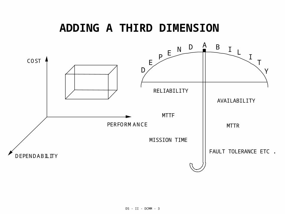
ADDING A THIRD DIMENSION

COST

DEPENDABILITY

PERFORMANCE

DE

PE N D A B I L

IT

Y

RELIABILITY

AVAILABILITY

MTTF

MTTR

MISSION TIME

FAULT TOLERANCE ETC .

DS - II - DCMM - 4

FAULT INTOLERANCE

• PRIOR ELIMINATION OF CAUSES OF UNRELIABILITY– fault avoidance– fault removal

• NO REDUNDANCY

• MANUAL / AUTOMATIC SYSTEM MAINTENANCE

• FAULT INTOLERANCE ATTAINS RELIABLE SYSTEMS BY:– very reliable components – refined design techniques– refined manufacturing techniques– shielding– comprehensive testing

DS - II - DCMM - 5

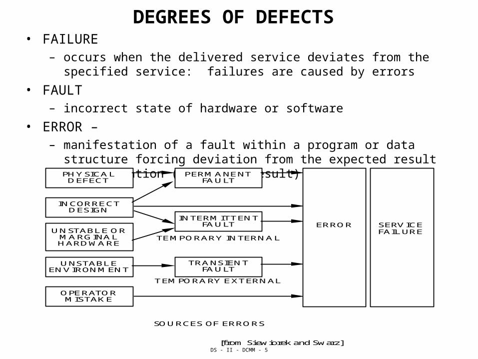
DEGREES OF DEFECTS • FAILURE

– occurs when the delivered service deviates from the specified service: failures are caused by errors

• FAULT – incorrect state of hardware or software 

• ERROR –– manifestation of a fault within a program or data structure forcing

deviation from the expected result of computation (incorrect result)PHYSICAL

DEFECTPERMANENT

FAULT

INCORRECT DESIGN

INTERMITTENT FAULT

UNSTABLE ENVIRONMENT

TRANSIENT FAULT

OPERATOR MISTAKE

UNSTABLE OR MARGINAL HARDWARE

SOURCES OF ERRORS

[from Siewiorek and Swarz]

TEMPORARY INTERNAL

TEMPORARY EXTERNAL

SERVICE FAILURE

ERROR

DS - II - DCMM - 6

TYPICAL FAULT MODELS FORPARALLEL / DISTRIBUTED SYSTEMS

• CRASH 

• OMISSION 

• TIMING 

• INCORRECT COMPUTATION /COMMUNICATION

• ARBITARARY (BYZANTINE)

DS - II - DCMM - 7

FAULT TOLERANCE: BENEFITS & DISADVANTAGE

• FAULT TOLERANCE – ACCEPT THAT AN IMPLEMENTED SYSTEM WILL NOT BE

FAULT-FREE

– FAULT TOLERANCE IS ATTAINED BY REDUNDANCY IN TIME AND/OR REDUNDANCY IN SPACE 

– AUTOMATIC RECOVERY FROM ERRORS 

– COMBINING REDUNDANCY AND FAULT INTOLERANCE 

• BENEFITS OF FAULT TOLERANCE– HIGHER RELIABILITY 

– LOWER TOTAL COST 

– PSYCHOLOGICAL SUPPORT OF USERS 

• DISADVANTAGE OF FAULT TOLERANCE – COST OF REDUNDANCY

DS - II - DCMM - 8

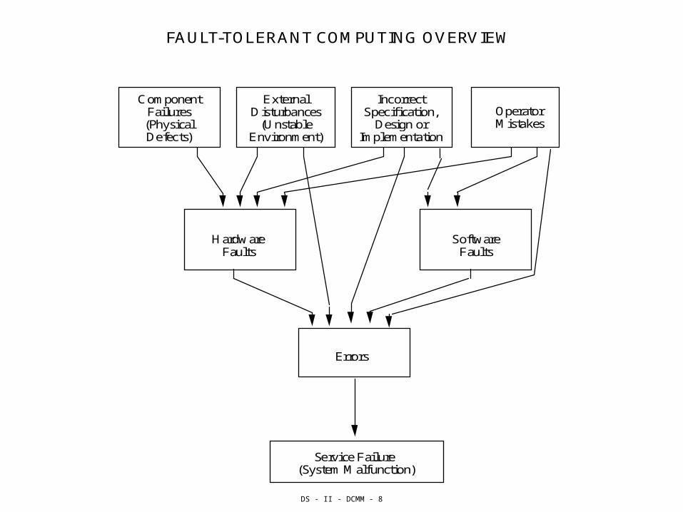
C o m p o n e n t F a i l u r e s ( P h y s i c a l D e f e c t s )

E x t e r n a l D i s t u r b a n c e s

( U n s t a b l e E n v i r o n m e n t )

O p e r a t o r M i s t a k e s

I n c o r r e c t S p e c i f i c a t i o n ,

D e s i g n o r I m p l e m e n t a t i o n

H a r d w a r e F a u l t s

S o f t w a r e F a u l t s

E r r o r s

F A U L T - T O L E R A N T C O M P U T I N G

O V E R V I E W

S e r v i c e F a i l u r e ( S y s t e m M a l f u n c t i o n )

DS - II - DCMM - 9

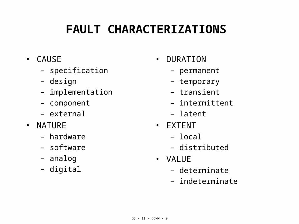
FAULT CHARACTERIZATIONS

• CAUSE– specification

– design

– implementation

– component

– external

• NATURE– hardware

– software

– analog

– digital

• DURATION– permanent

– temporary

– transient

– intermittent

– latent

• EXTENT – local

– distributed

• VALUE– determinate

– indeterminate

DS - II - DCMM - 10

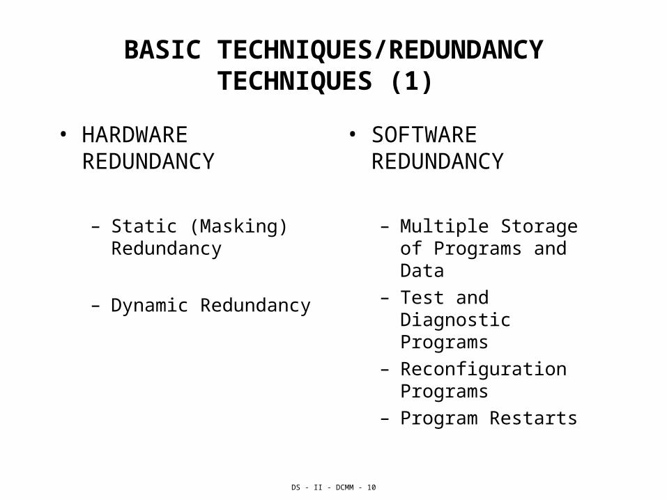
BASIC TECHNIQUES/REDUNDANCY TECHNIQUES (1)

• HARDWARE REDUNDANCY

– Static (Masking) Redundancy

– Dynamic Redundancy

• SOFTWARE REDUNDANCY

– Multiple Storage of Programs and Data

– Test and Diagnostic Programs

– Reconfiguration Programs

– Program Restarts

DS - II - DCMM - 11

BASIC TECHNIQUES/REDUNDANCY TECHNIQUES (2)

TIME (EXECUTION REDUNDANCY)

Repeat or acknowledge operations at various levels

Major Goal - Fault Detection and Recovery

DS - II - DCMM - 12

DEPENDABILITY MEASURES

• DEPENDABILITY IS A VALUE OF QUANTITATIVE MEASURES SUCH AS RELIABILITY AND AVAILABILITY AS PERCEIVED OR DEFINED BY A USER

• DEPENDABILITY IS THE QUALITY OF THE DELIVERED SERVICE SUCH THAT RELIANCE CAN JUSTIFIABLY BE PLACED ON THIS SERVICE

• DEPENDABILITY IS THE ABILITY OF A SYSTEM TO PERFORM A REQUIRED SERVICE UNDER STATED CONDITIONS FOR A SPECIFIED PERIOD OF TIME

DS - II - DCMM - 13

RELIABILITY

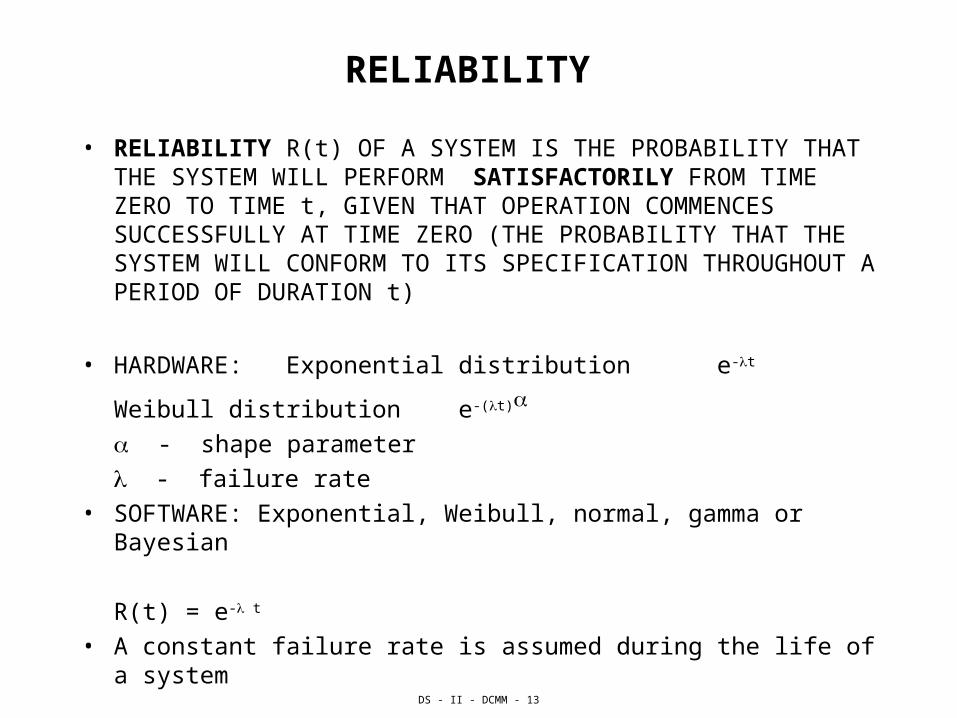
• RELIABILITY R(t) OF A SYSTEM IS THE PROBABILITY THAT THE SYSTEM WILL PERFORM SATISFACTORILY FROM TIME ZERO TO TIME t, GIVEN THAT OPERATION COMMENCES SUCCESSFULLY AT TIME ZERO (THE PROBABILITY THAT THE SYSTEM WILL CONFORM TO ITS SPECIFICATION THROUGHOUT A PERIOD OF DURATION t)

• HARDWARE: Exponential distribution e-t

Weibull distribution e-(t) - shape parameter - failure rate

• SOFTWARE: Exponential, Weibull, normal, gamma or Bayesian

R(t) = e- t

• A constant failure rate is assumed during the life of a system

DS - II - DCMM - 14

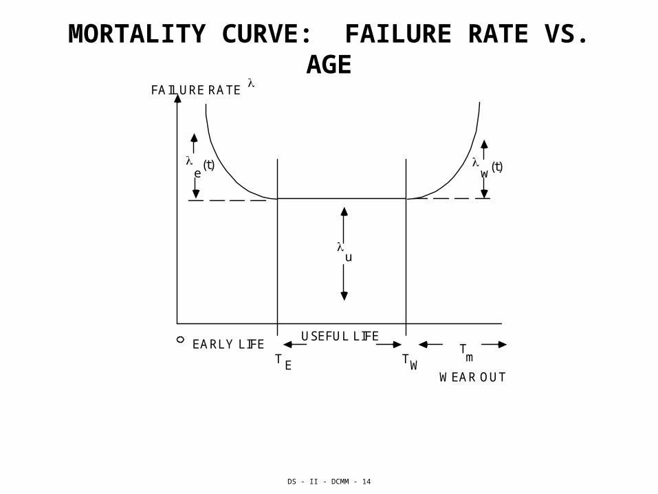
MORTALITY CURVE: FAILURE RATE VS. AGE FAILURE RATE

e (t) w

(t)

u

EARLY LIFE

T

USEFUL LIFE

T T

m E W

WEAR OUT

DS - II - DCMM - 15

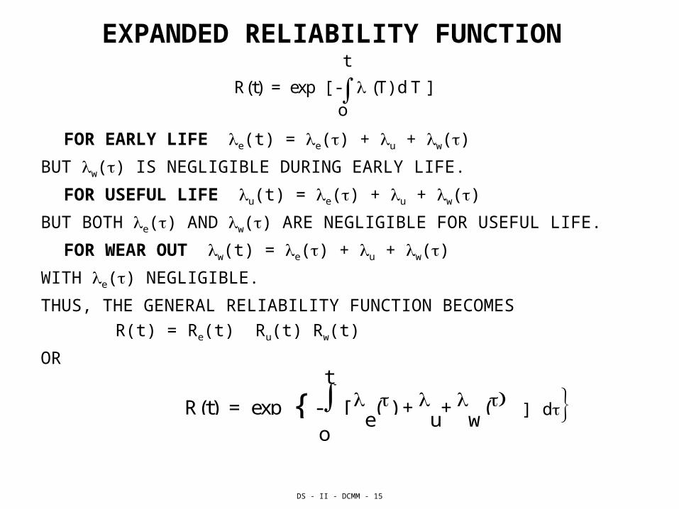
EXPANDED RELIABILITY FUNCTION

FOR EARLY LIFE e(t) = e() + u + w() 

BUT w() IS NEGLIGIBLE DURING EARLY LIFE. 

FOR USEFUL LIFE u(t) = e() + u + w() 

BUT BOTH e() AND w() ARE NEGLIGIBLE FOR USEFUL LIFE. 

FOR WEAR OUT w(t) = e() + u + w() 

WITH e() NEGLIGIBLE. 

THUS, THE GENERAL RELIABILITY FUNCTION BECOMES 

R(t) = Re(t) Ru(t) Rw(t)

OR

R(t) = exp [ -o

t

(T) d T ]

R ( t ) = e x p { - o

t

[ e ( ) +

u

+ w

( d] d

DS - II - DCMM - 16

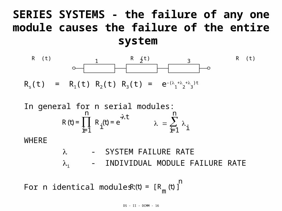
SERIES SYSTEMS - the failure of any one module causes the failure of the entire system

Rs(t) = R1(t) R2(t) R3(t) = e-(1

+2

+3

)t

In general for n serial modules:

WHERE 

- SYSTEM FAILURE RATE 

i - INDIVIDUAL MODULE FAILURE RATE

 

For n identical modules:

R (t) R (t) R (t)1 2 3

R(t) = i=1

n R

i(t) = e

-t

i=1

n

i

R(t) = [ Rm

(t) ]n

DS - II - DCMM - 17

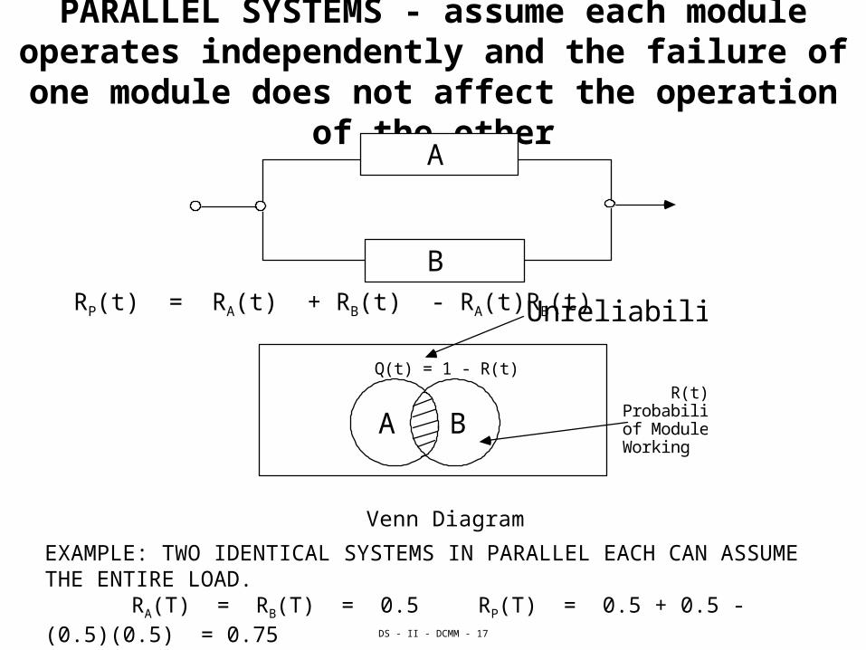
PARALLEL SYSTEMS - assume each module operates independently and the failure of one

module does not affect the operation of the other

RP(t) = RA(t) + RB(t) - RA(t)RB(t)

A

B

Unreliability

Q(t) = 1 - R(t)

A B R(t) Probability of Module Working

Venn Diagram

EXAMPLE: TWO IDENTICAL SYSTEMS IN PARALLEL EACH CAN ASSUME THE ENTIRE LOAD.

RA(T) = RB(T) = 0.5 RP(T) = 0.5 + 0.5 - (0.5)(0.5) = 0.75

DS - II - DCMM - 18

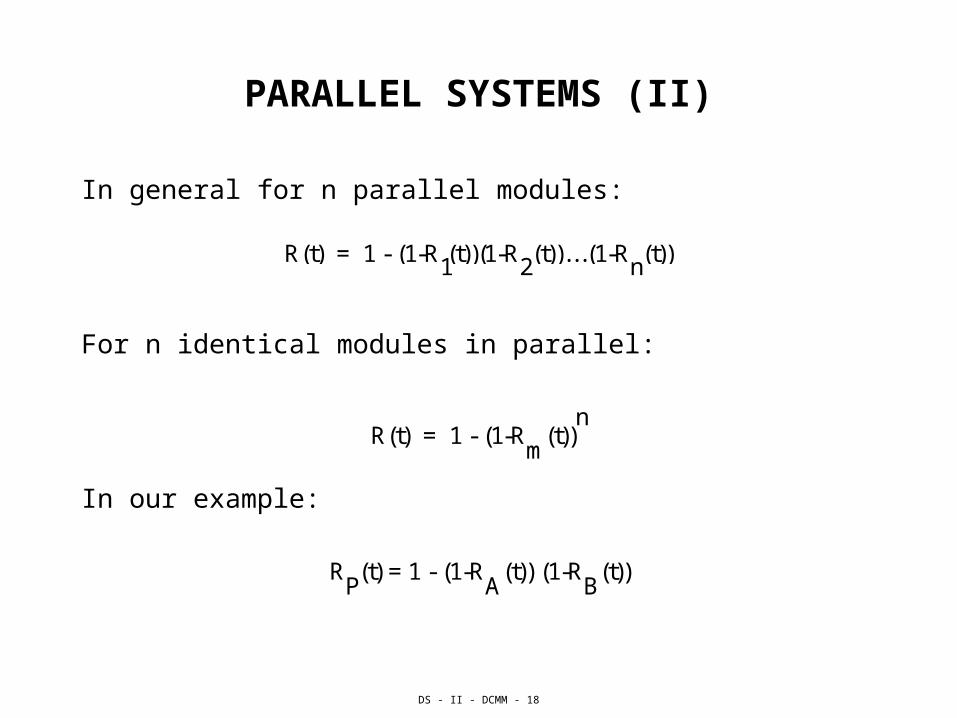
PARALLEL SYSTEMS (II)

In general for n parallel modules:

For n identical modules in parallel:

In our example:

R(t) = 1 - (1-R1i

(t))(1-R2(t)). . .(1-R

n(t))

R(t) = 1 - (1-Rm

(t))n

RP

(t) = 1 - (1-RA

(t)) (1-RB

(t))

DS - II - DCMM - 19

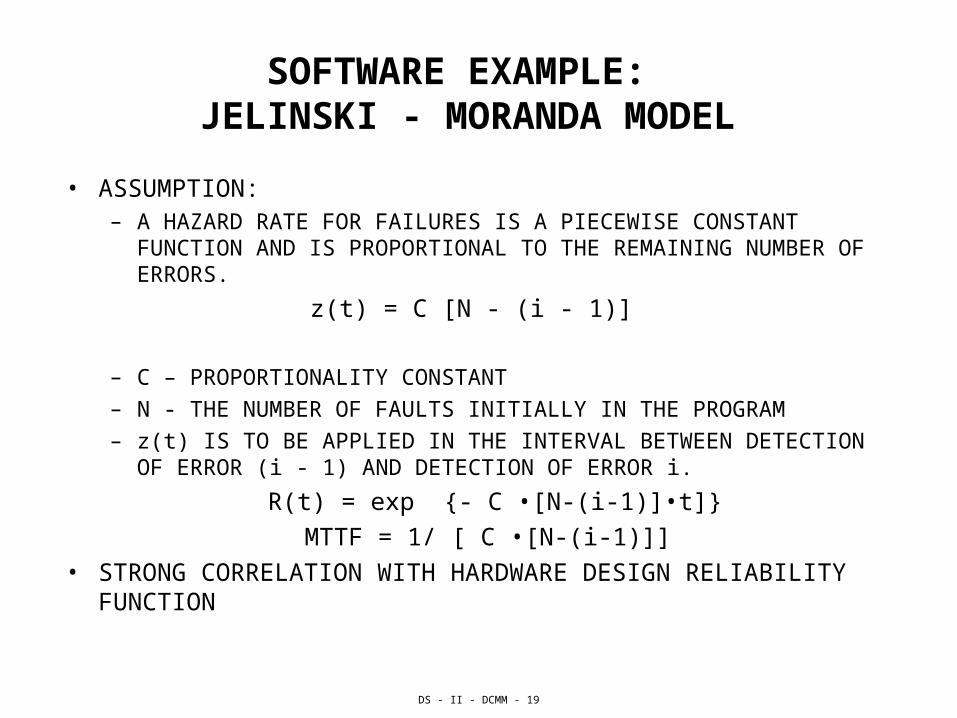
SOFTWARE EXAMPLE: JELINSKI - MORANDA MODEL

• ASSUMPTION: – A HAZARD RATE FOR FAILURES IS A PIECEWISE CONSTANT

FUNCTION AND IS PROPORTIONAL TO THE REMAINING NUMBER OF ERRORS.

z(t) = C [N - (i - 1)] 

– C – PROPORTIONALITY CONSTANT

– N - THE NUMBER OF FAULTS INITIALLY IN THE PROGRAM

– z(t) IS TO BE APPLIED IN THE INTERVAL BETWEEN DETECTION OF ERROR (i - 1) AND DETECTION OF ERROR i.

  R(t) = exp {- C •[N-(i-1)]•t]}

  MTTF = 1/ [ C •[N-(i-1)]] 

• STRONG CORRELATION WITH HARDWARE DESIGN RELIABILITY FUNCTION

DS - II - DCMM - 20

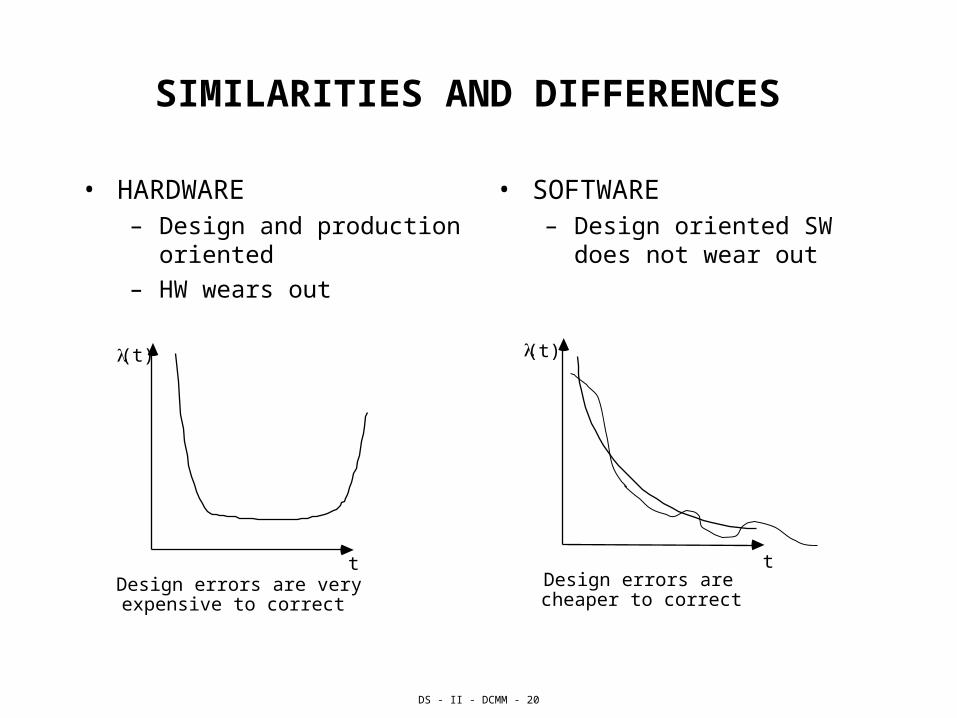
SIMILARITIES AND DIFFERENCES

• HARDWARE – Design and production

oriented

– HW wears out

• SOFTWARE– Design oriented SW does

not wear out

(t)

tDesign errors are very expensive to correct

(t)

t Design errors are cheaper to correct

DS - II - DCMM - 21

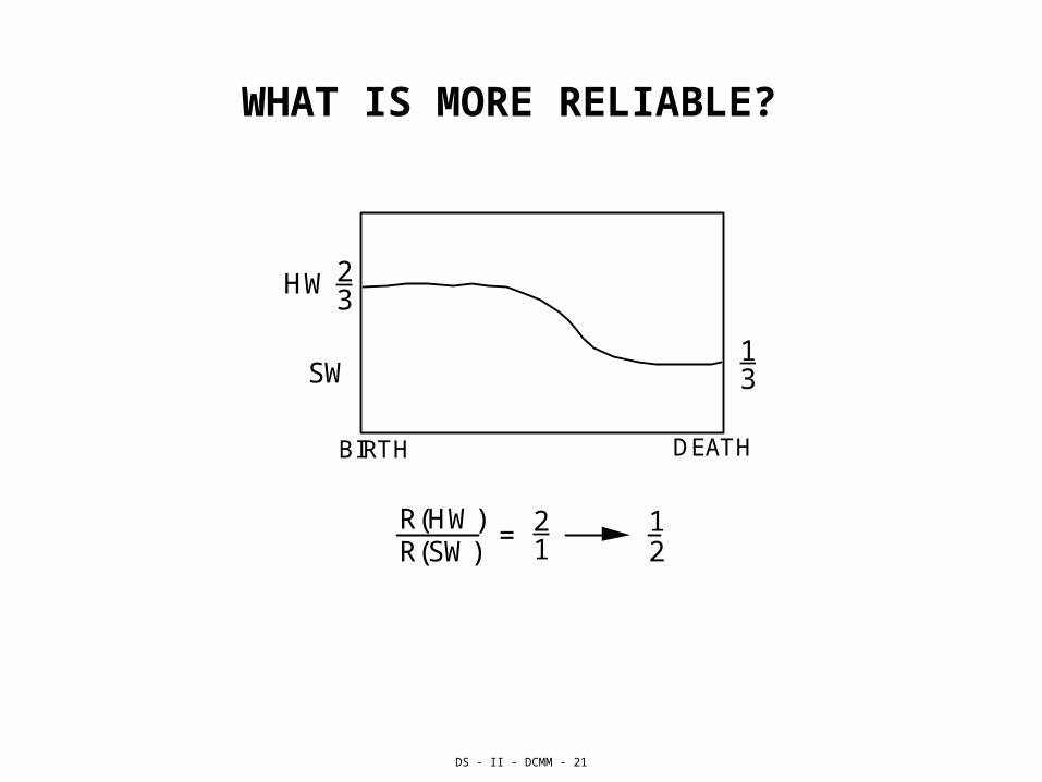
WHAT IS MORE RELIABLE?

HW 23

13SW

BIRTH DEATH

R(HW)R(SW)

= 21

12

DS - II - DCMM - 22

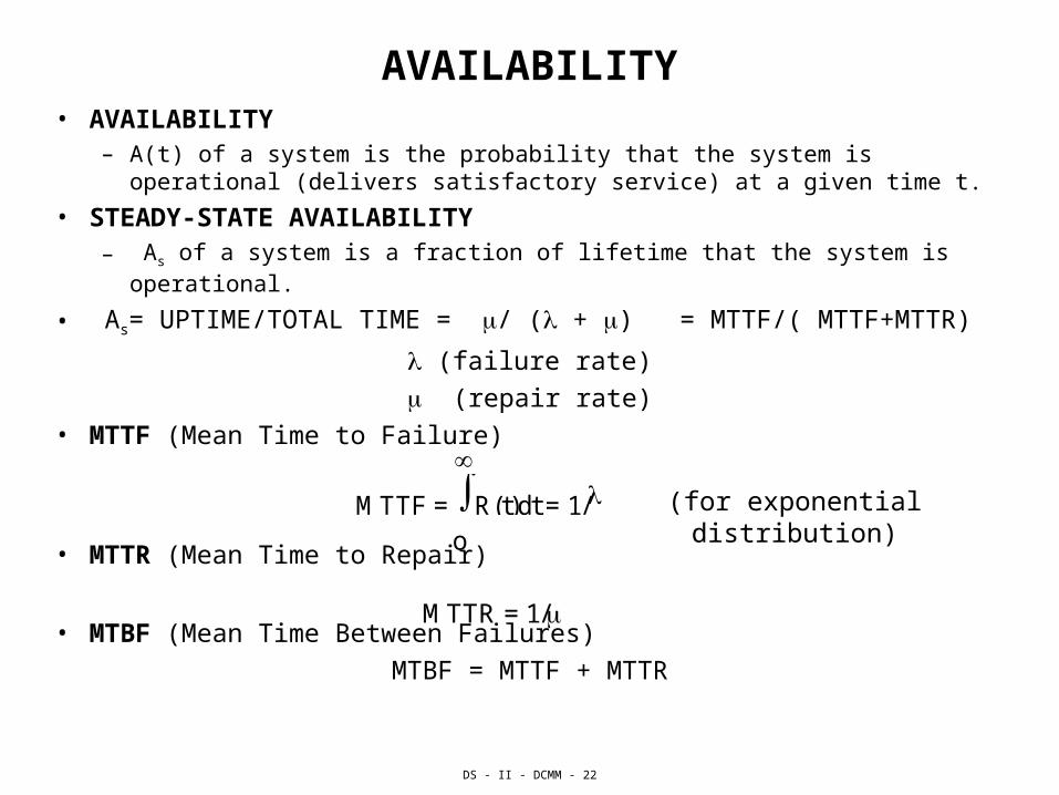
AVAILABILITY• AVAILABILITY

– A(t) of a system is the probability that the system is operational (delivers satisfactory service) at a given time t. 

• STEADY-STATE AVAILABILITY– As of a system is a fraction of lifetime that the system is operational. 

• As= UPTIME/TOTAL TIME = / ( + ) = MTTF/( MTTF+MTTR)

(failure rate)

(repair rate)• MTTF (Mean Time to Failure) 

• MTTR (Mean Time to Repair) 

• MTBF (Mean Time Between Failures)

MTBF = MTTF + MTTR

M T T F = o

R ( t ) d t = 1 /

MTTR = 1/

(for exponential distribution)

DS - II - DCMM - 23

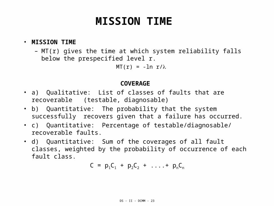
MISSION TIME

• MISSION TIME

– MT(r) gives the time at which system reliability falls below the prespecified level r.

MT(r) = -ln r/ 

COVERAGE 

• a) Qualitative: List of classes of faults that are recoverable (testable, diagnosable) 

• b) Quantitative: The probability that the system successfully recovers given that a failure has occurred. 

• c) Quantitative: Percentage of testable/diagnosable/ recoverable faults.  

• d) Quantitative: Sum of the coverages of all fault classes, weighted by the probability of occurrence of each fault class. 

C = p1C1 + p2C2 + ....+ pnCn

DS - II - DCMM - 24

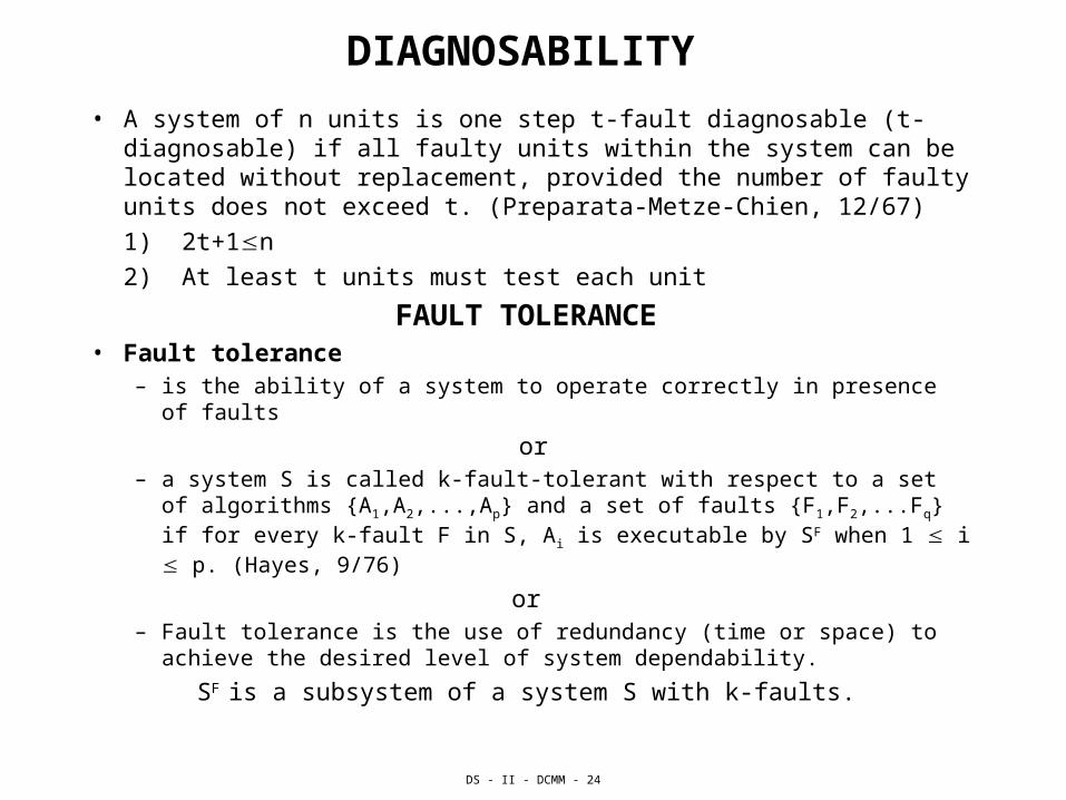
DIAGNOSABILITY

• A system of n units is one step t-fault diagnosable (t-diagnosable) if all faulty units within the system can be located without replacement, provided the number of faulty units does not exceed t. (Preparata-Metze-Chien, 12/67)

1) 2t+1n

2) At least t units must test each unit

FAULT TOLERANCE

• Fault tolerance – is the ability of a system to operate correctly in presence of faults

or– a system S is called k-fault-tolerant with respect to a set of algorithms

{A1,A2,...,Ap} and a set of faults {F1,F2,...Fq} if for every k-fault F in S, Ai is executable by SF when 1 i p. (Hayes, 9/76) 

or – Fault tolerance is the use of redundancy (time or space) to achieve

the desired level of system dependability. 

SF is a subsystem of a system S with k-faults.

DS - II - DCMM - 25

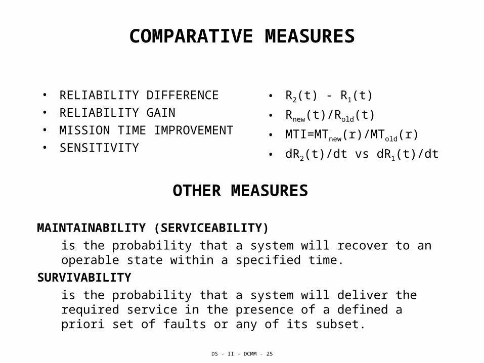
COMPARATIVE MEASURES

• RELIABILITY DIFFERENCE

• RELIABILITY GAIN  

• MISSION TIME IMPROVEMENT  

• SENSITIVITY  

• R2(t) - R1(t)

• Rnew(t)/Rold(t)

• MTI=MTnew(r)/MTold(r)

• dR2(t)/dt vs dR1(t)/dt

OTHER MEASURES 

MAINTAINABILITY (SERVICEABILITY)

is the probability that a system will recover to an operable state within a specified time.

SURVIVABILITY

is the probability that a system will deliver the required service in the presence of a defined a priori set of faults or any of its subset.

DS - II - DCMM - 26

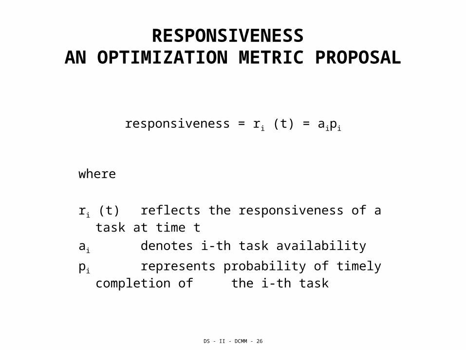
RESPONSIVENESS AN OPTIMIZATION METRIC PROPOSAL

responsiveness = ri (t) = aipi

where

ri (t) reflects the responsiveness of a task at time t

ai denotes i-th task availability

pi represents probability of timely completion of the i-th task

DS - II - DCMM - 27

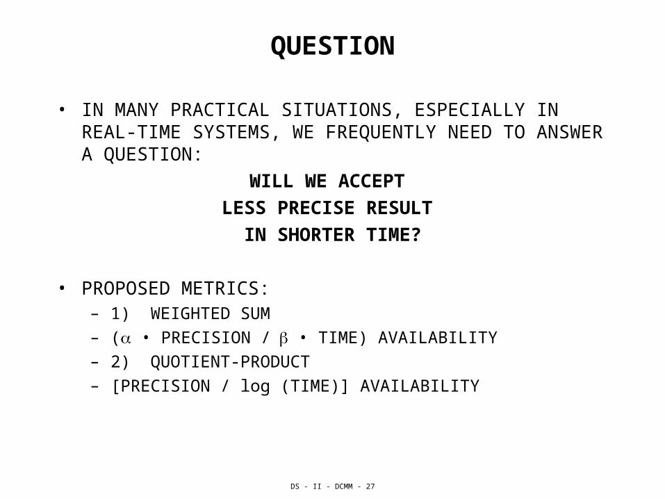
QUESTION

• IN MANY PRACTICAL SITUATIONS, ESPECIALLY IN REAL-TIME SYSTEMS, WE FREQUENTLY NEED TO ANSWER A QUESTION: 

WILL WE ACCEPT 

LESS PRECISE RESULT 

IN SHORTER TIME?

 • PROPOSED METRICS: 

– 1) WEIGHTED SUM 

– ( • PRECISION / • TIME) AVAILABILITY 

– 2) QUOTIENT-PRODUCT 

– [PRECISION / log (TIME)] AVAILABILITY

DS - II - DCMM - 28

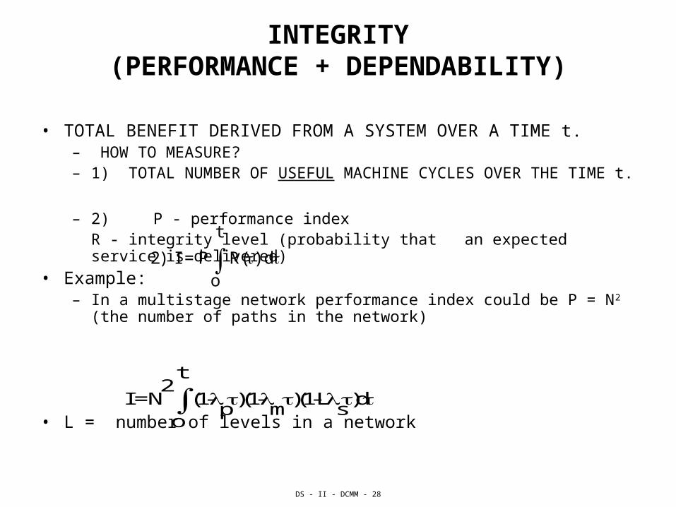
INTEGRITY(PERFORMANCE + DEPENDABILITY)

• TOTAL BENEFIT DERIVED FROM A SYSTEM OVER A TIME t.–  HOW TO MEASURE? – 1) TOTAL NUMBER OF USEFUL MACHINE CYCLES OVER THE TIME t.

– 2) P - performance index R - integrity level (probability

that an expected service is delivered) 

• Example: – In a multistage network performance index could be P = N2 (the number of

paths in the network)

• L = number of levels in a network

2) I = P o

t

R() d

I = N2 o

t

(1-p)(1-

m)(1-L

s)d

DS - II - DCMM - 29

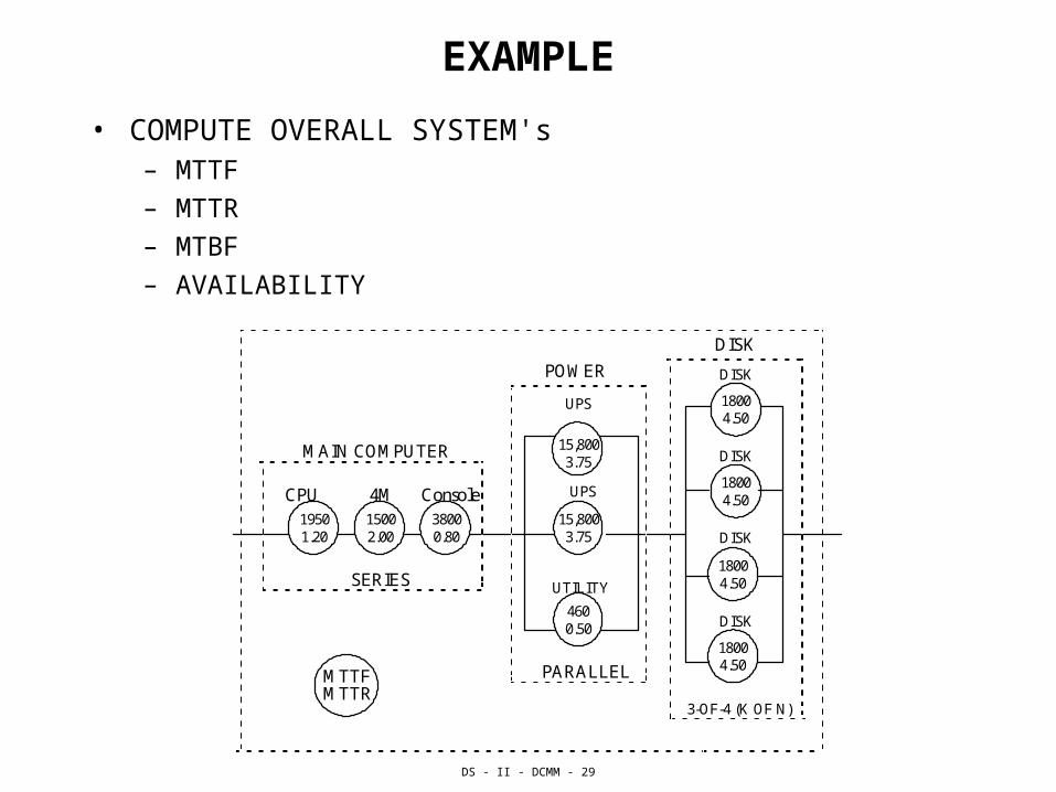
EXAMPLE

• COMPUTE OVERALL SYSTEM's – MTTF

– MTTR

– MTBF

– AVAILABILITY

DISK

POWER

MAIN COMPUTER

CPU 4M Console

1950 1.20

1500 2.00

3800 0.80

SERIES

PARALLEL

UPS

UPS

15,800 3.75

UTILITY

460 0.50

1800 4.50

1800 4.50

1800 4.50

1800 4.50

15,800 3.75

DISK

DISK

DISK

DISK

3-OF-4 (K OF N)

MTTF MTTR

DS - II - DCMM - 30

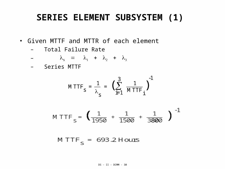
SERIES ELEMENT SUBSYSTEM (1)

• Given MTTF and MTTR of each element– Total Failure Rate 

– s

– Series MTTF

MTTFs =

s

1 = (

i=1

3

MTTF1

)-1

i

DS - II - DCMM - 31

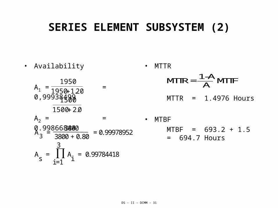
SERIES ELEMENT SUBSYSTEM (2)

• Availability

A1 = = 0,99938499

A2 = = 0.99866844

• MTTR

MTTR = 1.4976 Hours

• MTBF

MTBF = 693.2 + 1.5 = 694.7 Hours A

3 =

3800 + 0.803800

= 0.99978952

As =

i=1

3 A

i = 0.99784418

MTTR = A

1 - A MTTF

20.11950

1950

0.21500

1500

DS - II - DCMM - 32

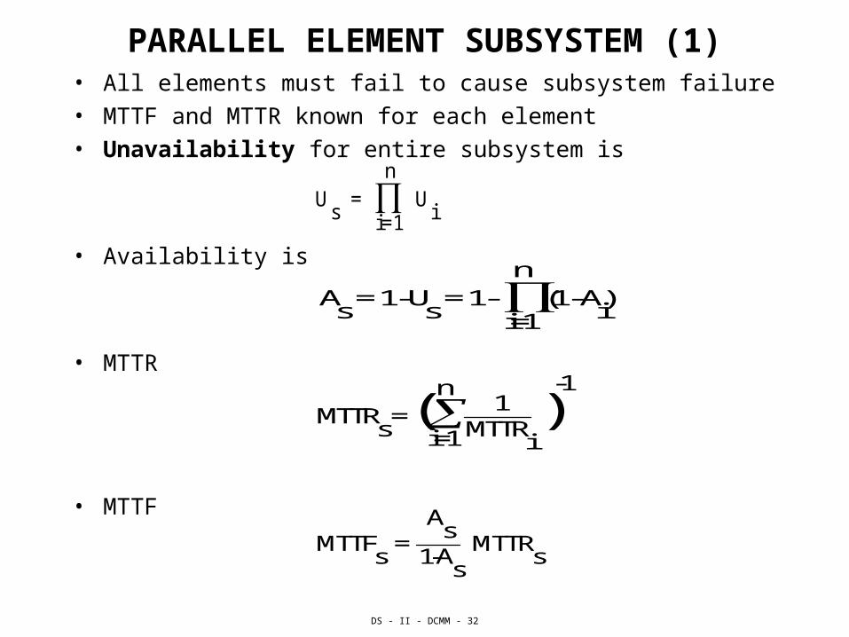
PARALLEL ELEMENT SUBSYSTEM (1)• All elements must fail to cause subsystem failure• MTTF and MTTR known for each element• Unavailability for entire subsystem is

• Availability is

• MTTR

• MTTF

Us =

i=1

n U

i

As = 1 - U

s = 1 -

i=1

n (1 - A

i)

MTTRs = (

i=1

n MTTR

i

1 )

-1

MTTFs =

1-As

As

MTTRs

DS - II - DCMM - 33

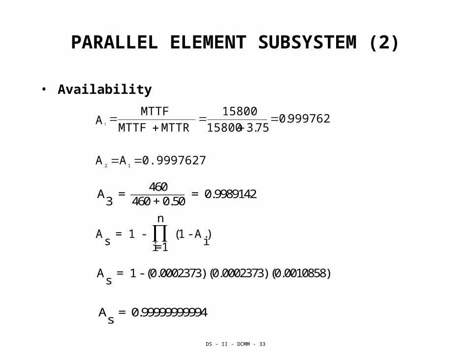
PARALLEL ELEMENT SUBSYSTEM (2)

• Availability

A3 =

460 + 0.50460

= 0.9989142

0.9997627 A A

9997627.075.315800

15800

MTTR MTTF

MTTF A

12

1

As = 1 -

i=1

n (1 - A

i)

As = 1 - (0.0002373) (0.0002373) (0.0010858)

As = 0.99999999994

DS - II - DCMM - 34

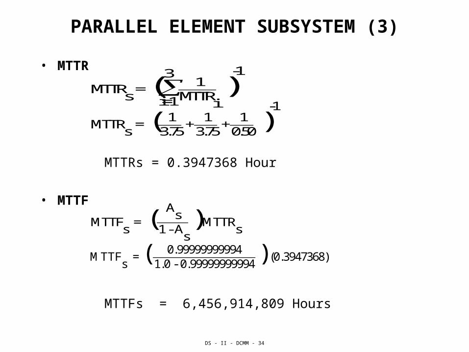
PARALLEL ELEMENT SUBSYSTEM (3)

• MTTR

MTTRs = 0.3947368 Hour

• MTTF

MTTFs = 6,456,914,809 Hours

MTTRs = (

i=1

3 MTTR

i

1 )

-1

MTTRs = (

3.751

+ 3.751

+ 0.501

)-1

MTTFs = (

1 - As

As

) MTTRs

MTTFs = (

1.0 - 0.999999999940.99999999994

) (0.3947368)

DS - II - DCMM - 35

PARALLEL ELEMENT SUBSYSTEM (4)

• Paralleling modules is a technique commonly used to significantly upgrade system reliability  

• Compare one universal power supply (UPS) with availability of 

0.9997627  

• to the parallel combination of power supplies with availability of 

0.99999999994 

• In practical systems availability ranges  (2 to 12 9‘s)

0.99 to 0.999999999999

DS - II - DCMM - 36

K of N PARALLEL ELEMENT SUBSYSTEM (1)

• Have N identical modules in parallel (assume all have the same MTTF and MTTR) 

• Only K elements are required for full operation • K = 1 is the same as parallel • K = N is the same as series 

• Reliability • Rs = Prob (system works for time T) = Prob (N modules work

or N - 1 modules work or . . . or K modules work)• Note: The above conditions are mutually exclusive • Rs = Prob (N modules work) + Prob (N - 1 modules work)

+ . . . + Prob (K modules work)

DS - II - DCMM - 37

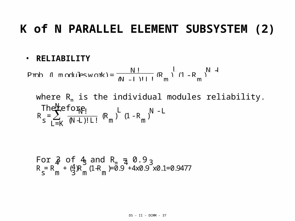
K of N PARALLEL ELEMENT SUBSYSTEM (2)

• RELIABILITY

where Rm is the individual modules reliability. Therefore

For 3 of 4 and Rm = 0.9

Rs =

L=K

N

(N-L)! L!N!

(Rm

)L

(1 - Rm

)N - L

Rs= R

m

4 + (

34)R

m

3(1-R

m)=0.9

4+4x0.9

3x0.1=0.9477

DS - II - DCMM - 38

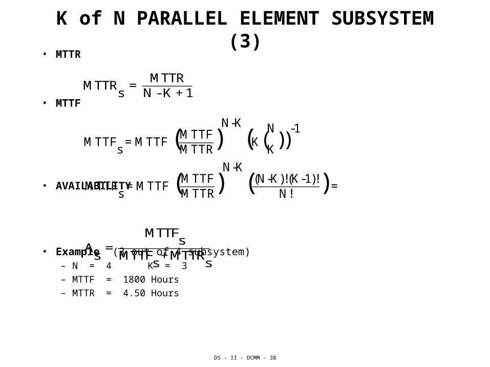
K of N PARALLEL ELEMENT SUBSYSTEM (3)• MTTR

• MTTF

• AVAILABILITY

• Example (3 out of 4 subsystem)– N = 4 K = 3 – MTTF = 1800 Hours – MTTR = 4.50 Hours

MTTRs =

N - K + 1MTTR

MTTFs = MTTF (

MTTRMTTF)

N-K

(K(K

N))

-1

MTTFs = MTTF (

MTTRMTTF)

N-K

(N!

(N-K)!(K-1)!) =

As =

MTTFs + MTTR

s

MTTFs

DS - II - DCMM - 39

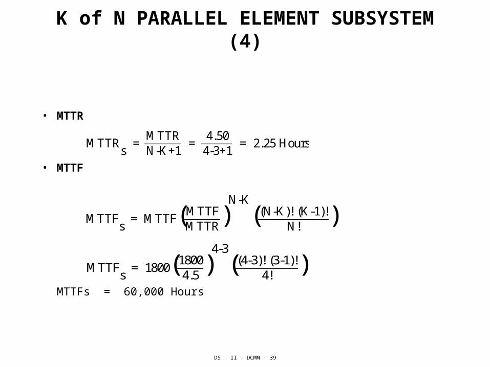
K of N PARALLEL ELEMENT SUBSYSTEM (4)

• MTTR

• MTTF

MTTFs = 60,000 Hours

MTTRs =

N-K+1MTTR

= 4-3+14.50

= 2.25 Hours

MTTFs = MTTF(

MTTRMTTF)

N-K

(N!

(N-K)! (K-1)!)

MTTFs = 1800(

4.51800)

4-3

(4!

(4-3)! (3-1)!)

DS - II - DCMM - 40

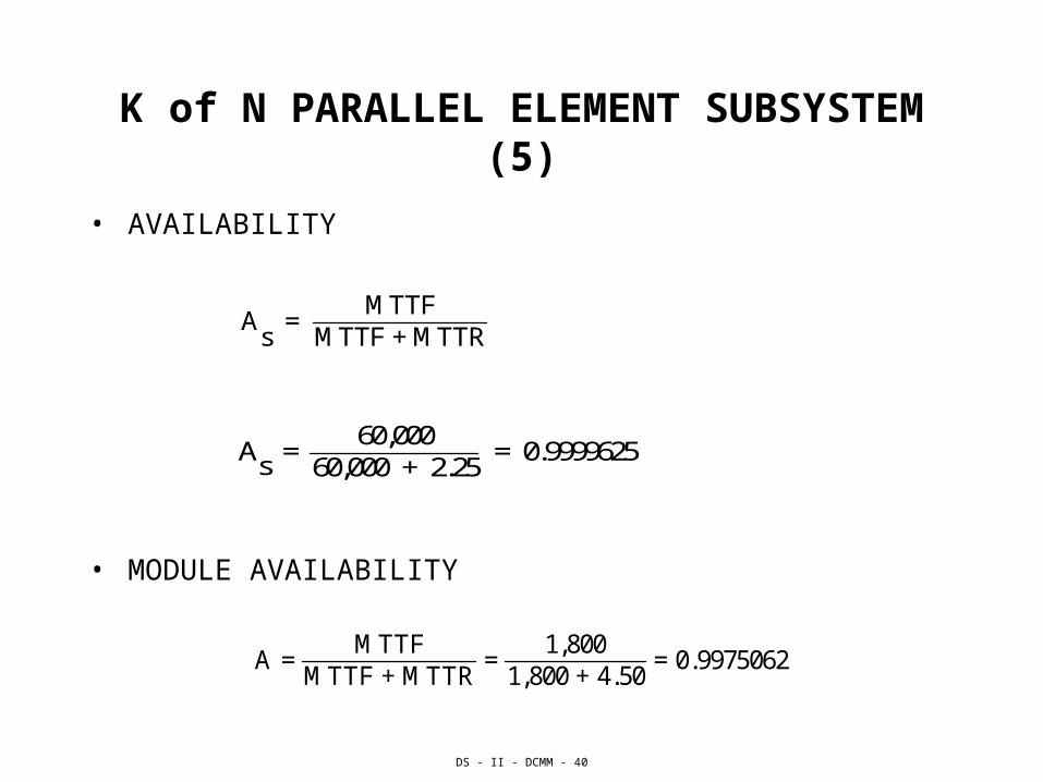
K of N PARALLEL ELEMENT SUBSYSTEM (5)

• AVAILABILITY

• MODULE AVAILABILITY

As =

MTTF + MTTRMTTF

As =

60,000 + 2.2560,000

= 0.9999625

A = MTTF + MTTR

MTTF =

1,800 + 4.501,800

= 0.9975062

DS - II - DCMM - 41

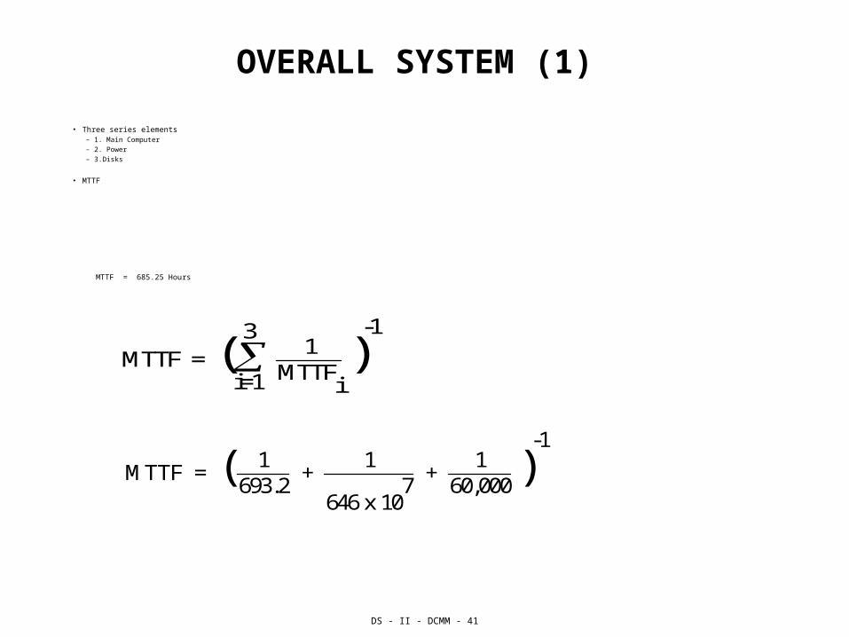
OVERALL SYSTEM (1)

• Three series elements– 1. Main Computer 

– 2. Power 

– 3.Disks

• MTTF

MTTF = 685.25 Hours

MTTF = ( i=1

3

MTTFi

1 )

-1

MTTF = ( 693.2

1 +

646 x 107

1 +

60,0001

)-1

DS - II - DCMM - 42

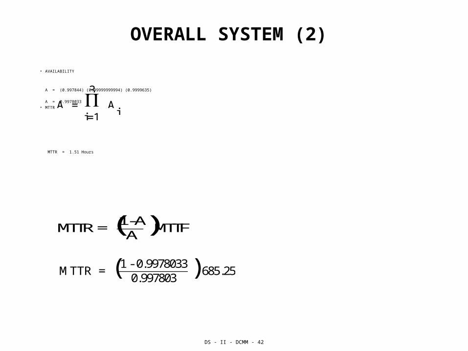
OVERALL SYSTEM (2)

• AVAILABILITY

A = (0.997844) (0.99999999994) (0.9999635)

 

A = 0.9978033• MTTR

MTTR = 1.51 Hours

A = i = 1

3 A

i

MTTR = (A

1 - A) MTTF

MTTR = (0.997803

1 - 0.9978033 ) 685.25

DS - II - DCMM - 43

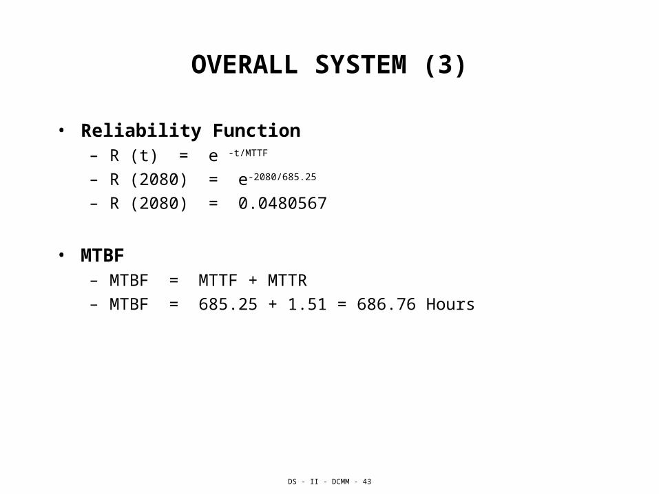
OVERALL SYSTEM (3)

• Reliability Function – R (t) = e -t/MTTF

– R (2080) = e-2080/685.25

– R (2080) = 0.0480567

 • MTBF

– MTBF = MTTF + MTTR

– MTBF = 685.25 + 1.51 = 686.76 Hours

DS - II - DCMM - 44

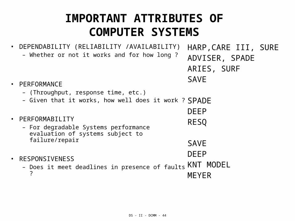
IMPORTANT ATTRIBUTES OF COMPUTER SYSTEMS

• DEPENDABILITY (RELIABILITY /AVAILABILITY) – Whether or not it works and for how long ?

• PERFORMANCE– (Throughput, response time, etc.) – Given that it works, how well does it work ?

• PERFORMABILITY – For degradable Systems performance evaluation

of systems subject to failure/repair

• RESPONSIVENESS – Does it meet deadlines in presence of faults ?

HARP,CARE III, SURE ADVISER, SPADE ARIES, SURF SAVE

SPADE DEEP RESQ

SAVEDEEP KNT MODEL MEYER

DS - II - DCMM - 45

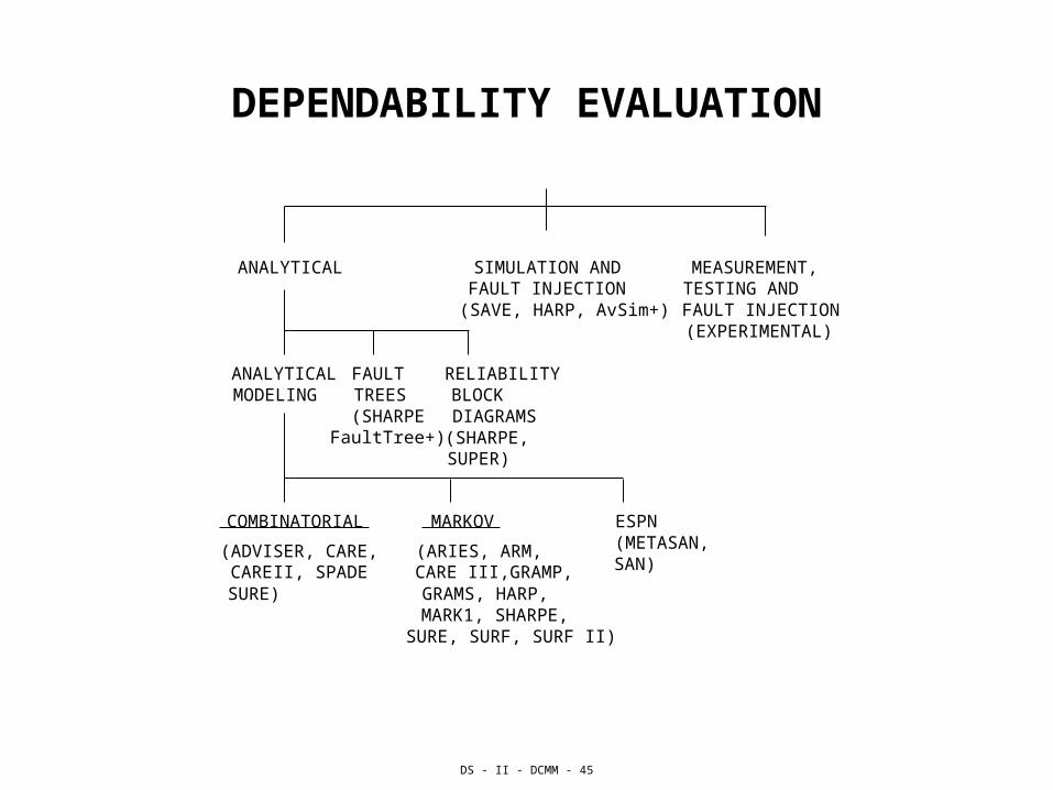
DEPENDABILITY EVALUATION

ANALYTICAL SIMULATION AND

FAULT INJECTION

(SAVE, HARP, AvSim+)

MEASUREMENT, TESTING AND FAULT INJECTION

(EXPERIMENTAL)

ANALYTICAL

MODELING

FAULT TREES

(SHARPEFaultTree+)

RELIABILITY

BLOCK

DIAGRAMS

(SHARPE, SUPER)

COMBINATORIAL

(ADVISER, CARE, CARE II, SPADE

SURE)

MARKOV

(ARIES, ARM, CARE III,GRAMP, GRAMS, HARP, MARK1, SHARPE, SURE, SURF, SURF II)

ESPN

(METASAN,SAN)

DS - II - DCMM - 46

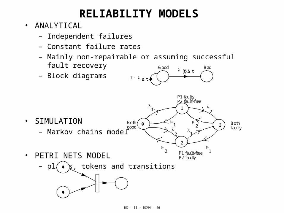
RELIABILITY MODELS • ANALYTICAL

– Independent failures

– Constant failure rates

– Mainly non-repairable or assuming successful fault recovery

– Block diagrams

• SIMULATION– Markov chains model

• PETRI NETS MODEL– places, tokens and transitions

Good Bad (t) Δ t

Δ t

1

3

2

0 Both faulty

P1 faulty P2 fault-free

Both good

P1 fault-free P2 faulty

1 2

2

1

1 2

2

1

DS - II - DCMM - 47

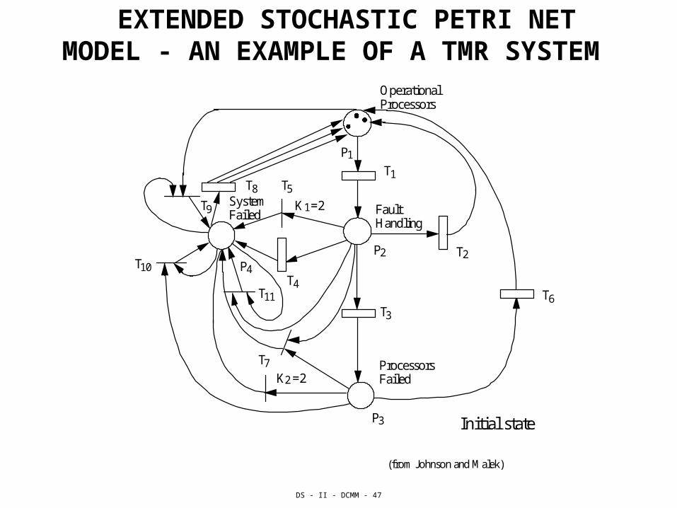
EXTENDED STOCHASTIC PETRI NET MODEL - AN EXAMPLE OF A TMR SYSTEM

Operational Processors

Fault Handling

System Failed

T 1

T 2

T 3

T 4

T 5

T 6

T 7

T 8

T 9

T 10

T 11

K =2 1

K =2 2

Processors Failed

P 1

P 2

P 3

P 4

Initial state

(from Johnson and Malek)

DS - II - DCMM - 48

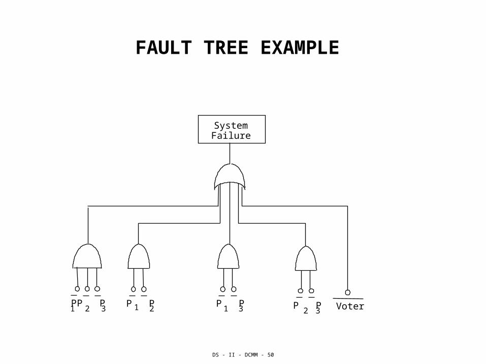
FAULT TREES

• Fault tree analysis is an application of deductive logic to produce a fault oriented pictorial diagram which allows one to analyze system safety and reliability. 

• Fault trees may serve as a design aid for identifying the general fault classes. 

• Fault trees were traditionally used in evaluation of hardware reliability but they may help in designing fault-tolerant software and in developing a top-down view of the system. 

• Complex event such as a system failure is consecutively broken down into simpler events such as subsystem failures, individual components and block failures, down to single element failures. These simple events are linked together by "and" or "or" Boolean functions. 

• The probability of higher level events can be calculated by combining probabilities of the lower level events.

DS - II - DCMM - 49

MARKOV MODELS

ARIES, CARE III, HARP, SAVE, SURE, SURF • Different Fault Types 

– Transient, Intermittent, Permanent

– Common-Mode

– Near-Coincident

• Details of Fault-Handling (Coverage) Behavior• Dynamic and Static Redundancy• Hierarchy is difficult to handle• State Explosion 

DS - II - DCMM - 50

FAULT TREE EXAMPLE

P P1 2P P

1 3 P P2 3 Voter

System Failure

P P1 2P

3

DS - II - DCMM - 51

HANDLING OF STATE SPACE PROBLEM

• BASIC APPROACH: – DIVIDE-AND-CONQUER (Decompose and Aggregate) 

 • STRUCTURAL DECOMPOSITION

– Consider a System as a Set of Independent Subsystems

• BEHAVIORAL DECOMPOSITION– Consider Different Time Constants in Fault-Occurrence and Fault-

Handling Processes

• Consider the Use of Different Techniques for Different Submodels

DS - II - DCMM - 52

RELIABILITY TOOLS OBJECTIVESAND TABLE OF COMPARISONS

• FAULT COVERAGE EVALUATION

 • RELIABILITY EVALUATION

• AVAILABILITY EVALUATION

• LIFE CYCLE EVALUATION

• MTTF/MTTR

• SERVICE COST

DS - II - DCMM - 53

EXPERIMENTAL

FAULT INJECTION

FAULT LATENCY

DEPENDABILITY MEASUREMENT

DS - II - DCMM - 54

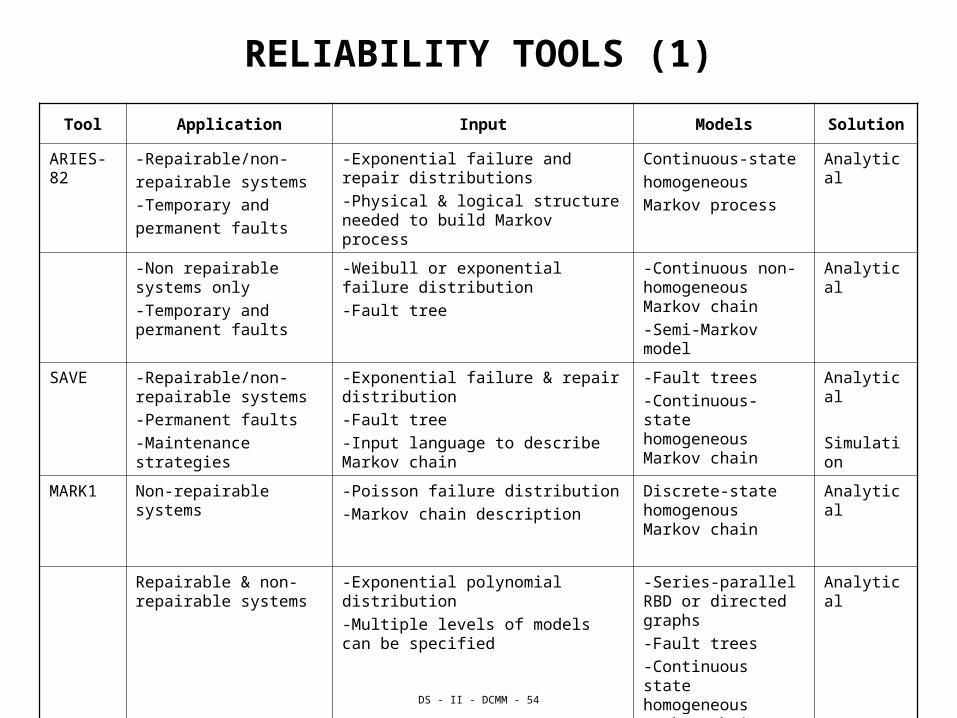
RELIABILITY TOOLS (1)

Tool Application Input Models Solution

ARIES-82

-Repairable/non-

repairable systems

-Temporary and

permanent faults

-Exponential failure and repair distributions

-Physical & logical structure needed to build Markov process

Continuous-state

homogeneous

Markov process

Analytical

-Non repairable systems only

-Temporary and permanent faults

-Weibull or exponential failure distribution

-Fault tree

-Continuous non- homogeneous Markov chain

-Semi-Markov model

Analytical

SAVE -Repairable/non-repairable systems

-Permanent faults

-Maintenance strategies

-Exponential failure & repair distribution

-Fault tree

-Input language to describe Markov chain

-Fault trees

-Continuous-state homogeneous Markov chain

Analytical

Simulation

MARK1 Non-repairable systems -Poisson failure distribution

-Markov chain description

Discrete-state homogenous Markov chain

Analytical

Repairable & non-repairable systems

-Exponential polynomial distribution

-Multiple levels of models can be specified

-Series-parallel RBD or directed graphs

-Fault trees

-Continuous state homogeneous Markov chain

-Semi-Markov chain

Analytical

DS - II - DCMM - 55

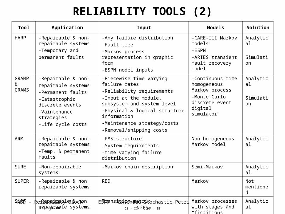
RELIABILITY TOOLS (2)Tool Application Input Models Solution

HARP -Repairable & non-repairable systems

-Temporary and

permanent faults

-Any failure distribution

-Fault tree

-Markov process representation in graphic form

-ESPN nodel inputs

-CARE-III Markov models

-ESPN

-ARIES transient fault recovery model

Analytical

Simulation

GRAMP & GRAMS

-Repairable & non-

repairable systems

-Permanent faults

-Catastrophic discrete events

-Vaintenance strategies

-Life cycle costs

-Piecewise time varying failure rates

-Reliability requirements

-Input at the module, subsystem and system level

-Physical & logical structure information

-Maintenance strategy/costs

-Removal/shipping costs

-Continuous-time homogeneous Markov process

-Monte Carlo discrete event digital simulator

Analytical

Simulation

ARM -Repairable & non-repairable systems

-Temp. & permanent faults

-PMS structure

-System requirements

-time varying failure distribution

Non homogeneous Markov model

Analytical

SURE -Non-repairable systems -Markov chain description Semi-Markov Analytical

SUPER -Repairable & non repairable systems

RBD Markov Not mentioned

SURF -Repairable & non repairable systems

Transition matrix Markov processes with stages and “fictitious” events

Analytical

META-SAN

-Non-repairable systems Description of Stochastic Activity Network

Stochastic Activity Networks

Analytical Simulation

RBD - Reliability Block Diagram ESPN - Extended Stochastic Petri Nets

DS - II - DCMM - 56

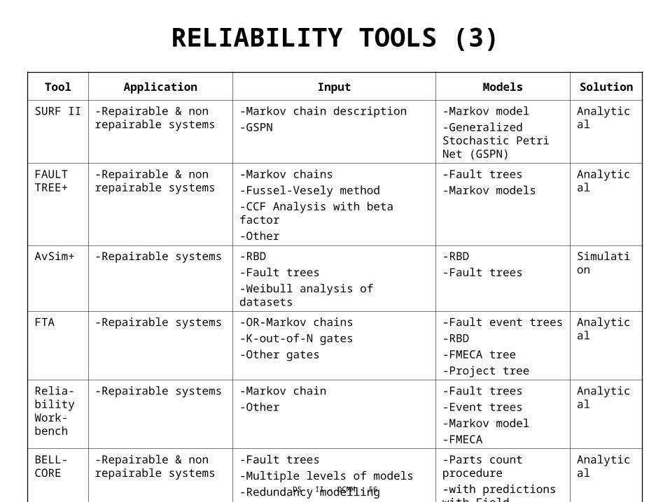
RELIABILITY TOOLS (3)

Tool Application Input Models Solution

SURF II -Repairable & non repairable systems

-Markov chain description

-GSPN

-Markov model

-Generalized Stochastic Petri Net (GSPN)

Analytical

FAULT TREE+

-Repairable & non repairable systems

-Markov chains

-Fussel-Vesely method

-CCF Analysis with beta factor

-Other

-Fault trees

-Markov models

Analytical

AvSim+ -Repairable systems -RBD

-Fault trees

-Weibull analysis of datasets

-RBD

-Fault trees

Simulation

FTA -Repairable systems -OR-Markov chains

-K-out-of-N gates

-Other gates

-Fault event trees

-RBD

-FMECA tree

-Project tree

Analytical

Relia-bility Work-bench

-Repairable systems -Markov chain

-Other

-Fault trees

-Event trees

-Markov model

-FMECA

Analytical

BELL-CORE

-Repairable & non repairable systems

-Fault trees

-Multiple levels of models

-Redundancy modelling

-Parts count procedure

-with predictions with Field Tracking Data

-Other

Analytical

DS - II - DCMM - 57

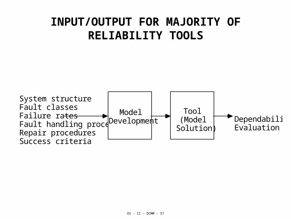
INPUT/OUTPUT FOR MAJORITY OF RELIABILITY TOOLS

System structure Fault classes Failure rates Fault handling procedures Repair procedures Success criteria

Dependability Evaluation

Model Development

Tool (Model

Solution)

DS - II - DCMM - 58

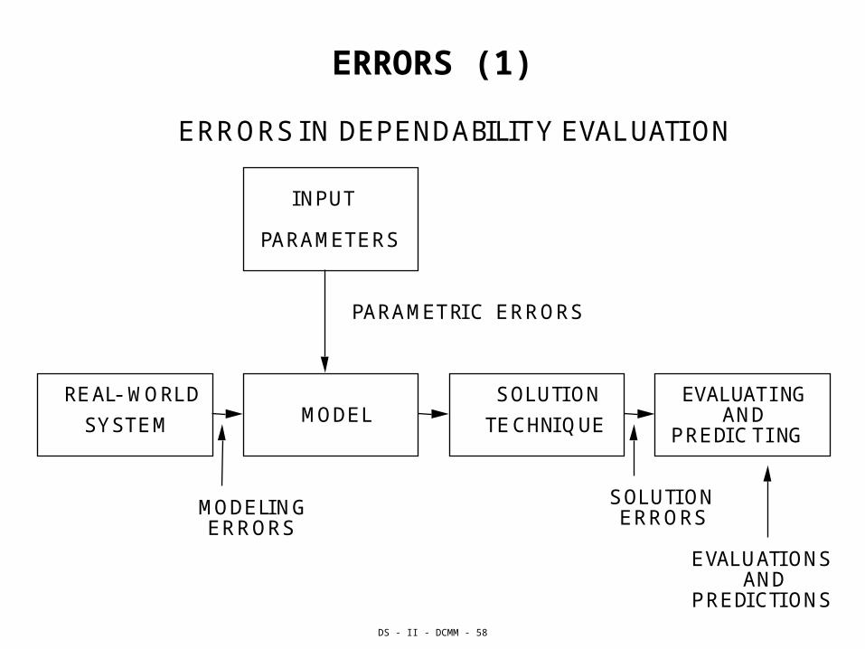
ERRORS (1)

ERRORS IN DEPENDABILITY EVALUATION

INPUT

PARAMETERS

REAL-WORLD

SYSTEM MODELSOLUTION

TECHNIQUE

EVALUATINGAND

PREDIC TING

SOLUTIONERRORS

EVALUATIONSAND

PREDICTIONS

MODELINGERRORS

PARAMETRIC ERRORS

DS - II - DCMM - 59

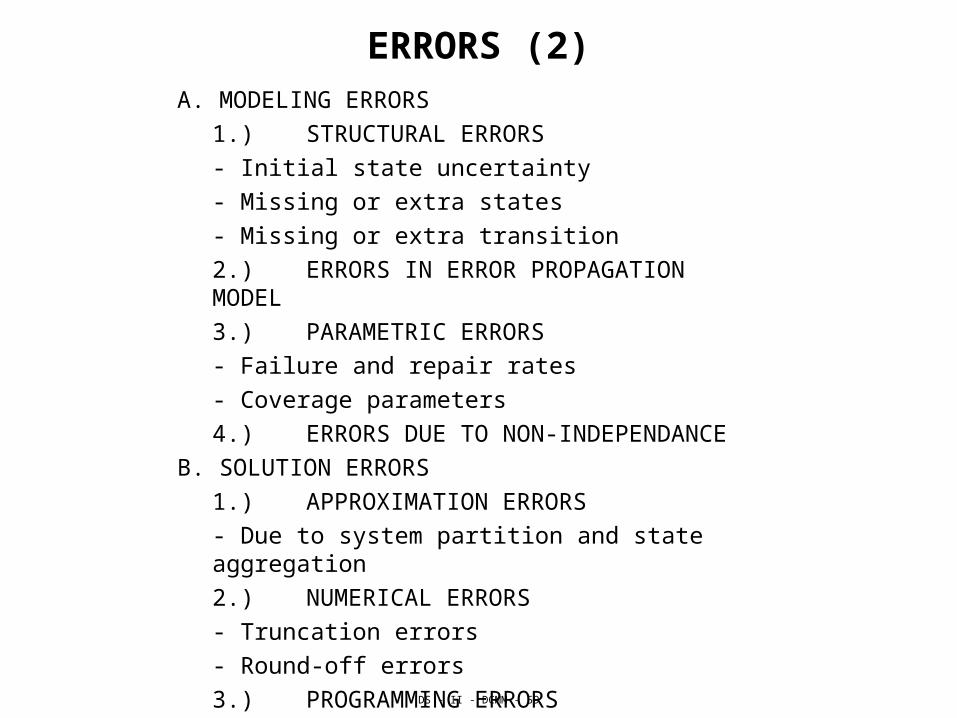
ERRORS (2)A. MODELING ERRORS 

1.) STRUCTURAL ERRORS

- Initial state uncertainty

- Missing or extra states

- Missing or extra transition 

2.) ERRORS IN ERROR PROPAGATION MODEL 

3.) PARAMETRIC ERRORS

- Failure and repair rates

- Coverage parameters 

4.) ERRORS DUE TO NON-INDEPENDANCE 

B. SOLUTION ERRORS 

1.) APPROXIMATION ERRORS

- Due to system partition and state aggregation 

2.) NUMERICAL ERRORS

- Truncation errors

- Round-off errors 

3.) PROGRAMMING ERRORS

DS - II - DCMM - 60

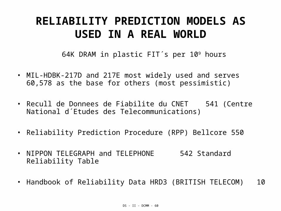
RELIABILITY PREDICTION MODELS ASUSED IN A REAL WORLD

64K DRAM in plastic FIT´s per 109 hours

• MIL-HDBK-217D and 217E most widely used and serves 60,578 as the base for others (most pessimistic)

• Recull de Donnees de Fiabilite du CNET 541 (Centre National d´Etudes des Telecommunications)

• Reliability Prediction Procedure (RPP) Bellcore 550

• NIPPON TELEGRAPH and TELEPHONE 542 Standard Reliability Table

• Handbook of Reliability Data HRD3 (BRITISH TELECOM) 10

DS - II - DCMM - 61

MIL-HDBK-217E RELIABILITY MODEL

• The MIL-217 Module is a powerful reliability prediction program based on the internationally recognised method of calculating electronic equipment reliability given in MIL-HDBK-217. This standard uses a series of models for various categories of electronic, electrical and electro-mechanical components to predict failure rates which are affected by environmental conditions, quality levels, stress conditions and various other parameters. These models are fully detailed in MIL-HDBK-217.

• Multi Systems within the same Project• Transfer to and from any other module• Linked Blocks, represent blocks with identical characteristics• Redundancy modelling including hot standby• Mission Phase• Additional sources

– http://www.t-cubed.com/faq_217.htm– http://www.relexsoftware.com/

DS - II - DCMM - 62

SUMMARY OF MIL-HDBK-217E RELIABILITY MODEL

FAILURE RATE MODEL AND FACTORS

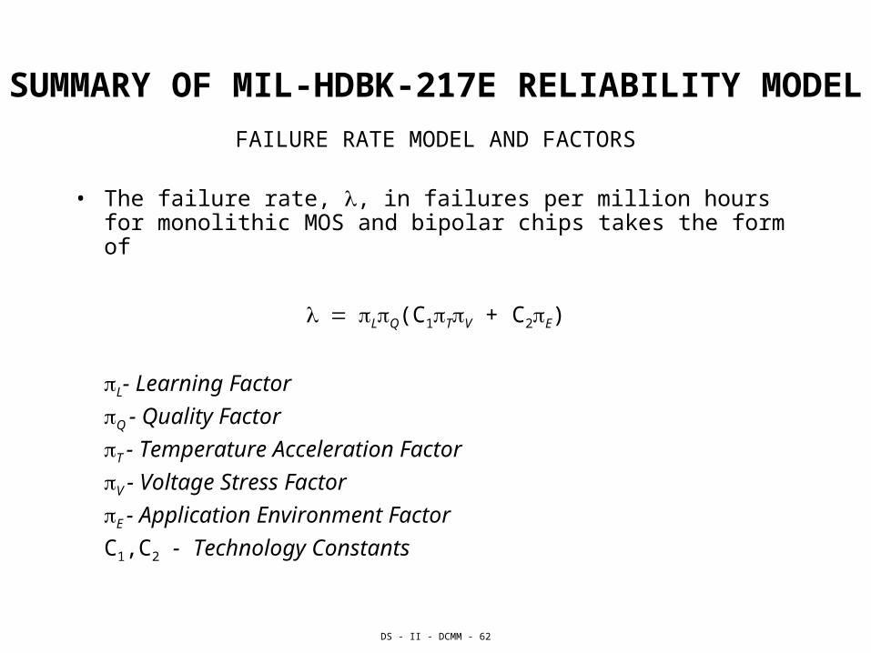
• The failure rate, , in failures per million hours for monolithic MOS and bipolar chips takes the form of

LQ(C1TV + C2E)

L- Learning Factor Q - Quality Factor T - Temperature Acceleration Factor V - Voltage Stress Factor E - Application Environment Factor C1,C2 - Technology Constants

DS - II - DCMM - 63

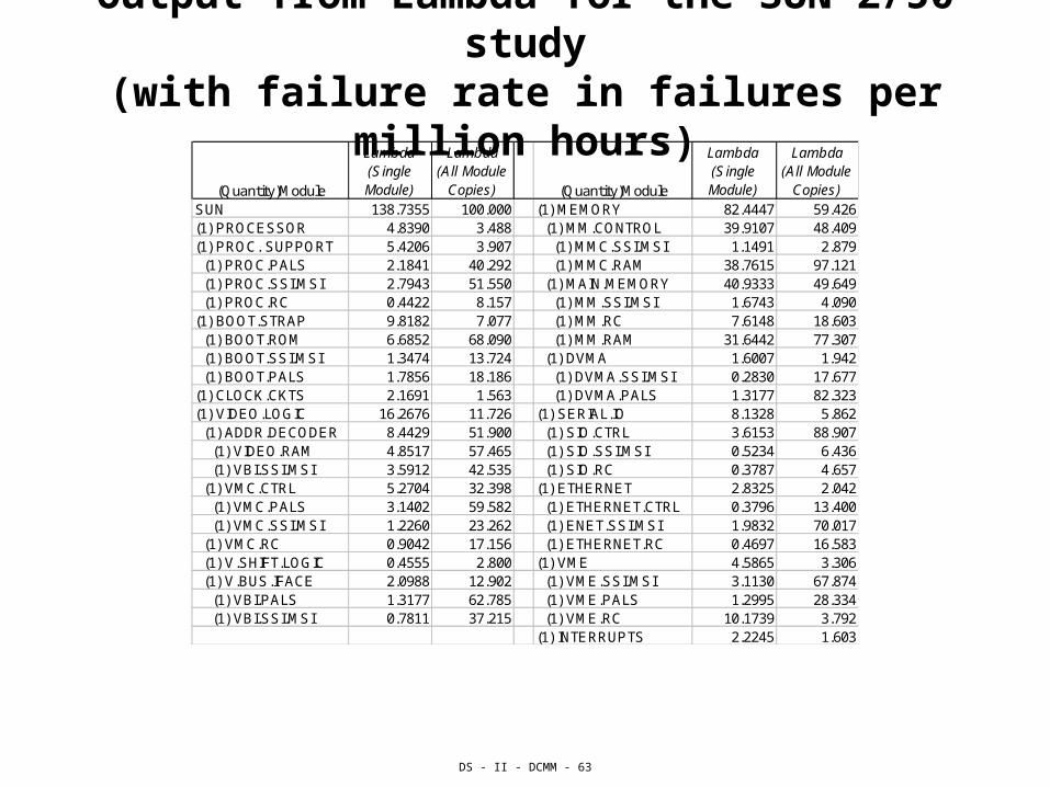
Output from Lambda for the SUN-2/50 study(with failure rate in failures per million hours)

(Quantity)Module

Lambda (Single Module)

Lambda(All Module

Copies) (Quantity)Module

Lambda (Single Module)

Lambda(All Module

Copies)SUN 138.7355 100.000 (1) MEMORY 82.4447 59.426(1) PROCESSOR 4.8390 3.488 (1) MM.CONTROL 39.9107 48.409(1) PROC. SUPPORT 5.4206 3.907 (1) MMC.SSI.MSI 1.1491 2.879 (1) PROC.PALS 2.1841 40.292 (1) MMC.RAM 38.7615 97.121 (1) PROC.SSI.MSI 2.7943 51.550 (1) MAIN.MEMORY 40.9333 49.649 (1) PROC.RC 0.4422 8.157 (1) MM.SSI.MSI 1.6743 4.090(1) BOOT.STRAP 9.8182 7.077 (1) MM.RC 7.6148 18.603 (1) BOOT.ROM 6.6852 68.090 (1) MM.RAM 31.6442 77.307 (1) BOOT.SSI.MSI 1.3474 13.724 (1) DVMA 1.6007 1.942 (1) BOOT.PALS 1.7856 18.186 (1) DVMA.SSI.MSI 0.2830 17.677(1) CLOCK.CKTS 2.1691 1.563 (1) DVMA.PALS 1.3177 82.323(1) VIDEO.LOGIC 16.2676 11.726 (1) SERIAL.IO 8.1328 5.862 (1) ADDR.DECODER 8.4429 51.900 (1) SIO.CTRL 3.6153 88.907 (1) VIDEO.RAM 4.8517 57.465 (1) SIO.SSI.MSI 0.5234 6.436 (1) VBI.SSI.MSI 3.5912 42.535 (1) SIO.RC 0.3787 4.657 (1) VMC.CTRL 5.2704 32.398 (1) ETHERNET 2.8325 2.042 (1) VMC.PALS 3.1402 59.582 (1) ETHERNET.CTRL 0.3796 13.400 (1) VMC.SSI.MSI 1.2260 23.262 (1) ENET.SSI.MSI 1.9832 70.017 (1) VMC.RC 0.9042 17.156 (1) ETHERNET.RC 0.4697 16.583 (1) V.SHIFT.LOGIC 0.4555 2.800 (1) VME 4.5865 3.306 (1) V.BUS.IFACE 2.0988 12.902 (1) VME.SSI.MSI 3.1130 67.874 (1) VBI.PALS 1.3177 62.785 (1) VME.PALS 1.2995 28.334 (1) VBI.SSI.MSI 0.7811 37.215 (1) VME.RC 10.1739 3.792

(1) INTERRUPTS 2.2245 1.603

DS - II - DCMM - 64

BELLCOR´S RELIABILITY PREDICTION PROGRAM• The Bellcore Module calculates the reliability prediction of electronic

equipment based on the Bellcore (Telcordia) standard TR-332 Issue 6. This standard uses a series of models for various categories of electronic, electrical and electro-mechanical components to predict steady-state failure rates which are affected by environmental conditions, quality levels, electrical stress conditions and various other parameters. These models allow reliability prediction to be performed using three methods.

• Method I : Parts Count procedure • Method II : Combines Method I predictions with laboratory data • Method III : Combines Method I predictions with Field Tracking Data • Multi Systems within the same Project • Transfer to and from any other module • Linked Blocks, represent blocks with identical characteristics • Redundancy modelling including hot standby• Global Editing• Additional source

– http://www.relexsoftware.com/

DS - II - DCMM - 65

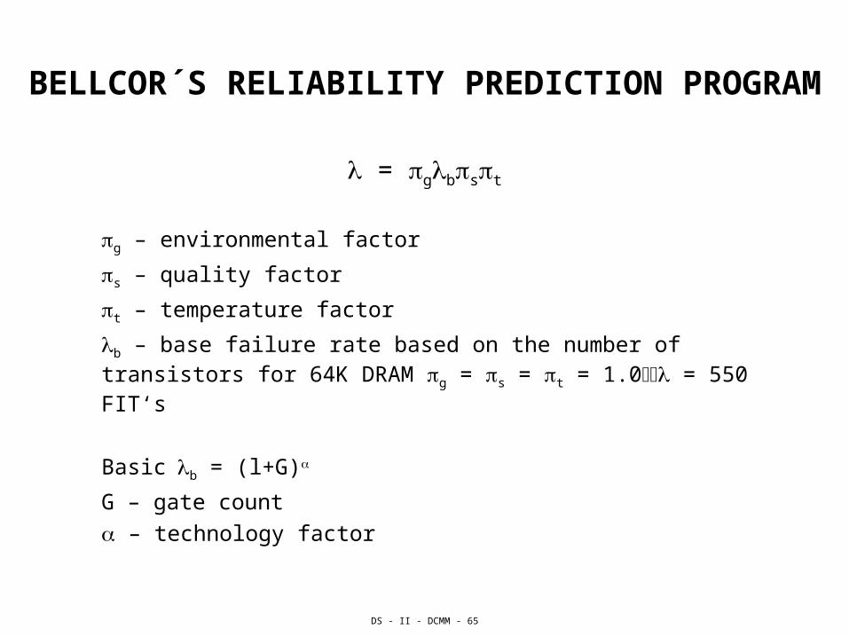
BELLCOR´S RELIABILITY PREDICTION PROGRAM

= gbst

g – environmental factor

s – quality factor

t – temperature factor

b – base failure rate based on the number of transistors for 64K DRAM g = s = t = 1.0 = 550 FIT‘s

Basicb = (l+G)

G – gate count

– technology factor

DS - II - DCMM - 66

REFERENCES:

• A. M. Johnson and M. Malek, "Survey of Software Tools for Evaluating Reliability, Availability and Serviceability," ACM Computing Surveys, 20 (4), 227-269, December 1988; translated and reprinted in Japanese, Kyoritsu Shuppan Co., Ltd., publisher, 1990.

• R. Geist, M. Smotherman, and M. Brown, "Ultrahigh Reliability Estimates for Systems Exhibiting Globally Time-Dependent Failure Processes", Proceedings of the 19th IEEE International Symposium on Fault-Tolerant Computing (FTCS-19), 152-158, Chicago, IL, June 1989.

• Software Quality and Reliability: Tools and Methods (Unicom Applied Information Technology Reports) Darrell Ince(Editor) / Hardcover/Published 1991.